1.1

Chapter 1. Introduction

1.1 Background

Recent research has shown that deterioration in thick, well constructed flexible

pavement structures (typical of UK trunk roads and motorways) is confined to the

surfacing, in the form of rutting and surface-initiated cracking. If timely treatment is

applied, this deterioration has been found not to significantly affect the structural

integrity of the pavement, which has led to the concept of “long life” pavements

[Nunn, 1997]. In parallel with this, there has been a general trend in the UK to use

progressively stiffer base materials, driven by the need to minimise costly

maintenance interventions, frequently in combination with one of the new generation

of thin surfacing materials.

Initial road trials of High Modulus Base (referred to as HMB) materials containing a

15 Penetration bitumen (10/20 paving grade), known as HMB15, were undertaken in

the UK at five sites [Nunn and Smith, 1997]. Results demonstrated that HMB15

behaved in a similar way to conventional base macadams, provided that appropriate

mixing, laying and compaction temperatures were maintained. Due to the high

stiffness modulus of this material it was estimated that cost savings of approximately

25% could be achieved compared to laying conventional Dense Bitumen Macadam

(DBM).

However, on-going monitoring of an initial trial site, located at the Transport

Research Laboratory (TRL), showed that the stiffness modulus had unexpectedly

dropped by approximately 60% after about 8 years. Since the HMB15 base layer at

this site had not been surfaced or trafficked it was thought that the drop in stiffness

modulus was due to moisture and air which had been allowed to permeate into the

material. As a comparison, other investigations have been performed on several in-

service pavements containing HMB materials. Results showed that these pavements

generally performed better than the TRL trial site, although a small number also

showed an unexpected drop in stiffness modulus. Investigations on cored samples

from the site also clearly demonstrated a certain level of visual deterioration, mainly

1.2

in the upper base layer. Some of the results from one such core investigation are

presented in Appendix A.

Due to these concerns over long-term durability (ageing and moisture) the Highways

Agency (HA) temporarily suspended the use of HMB materials containing 15

Penetration (10/20 paving grade) and 25 Penetration (20/30 paving grade) bitumens

and established a research programme, led by Scott Wilson Pavement Engineering

(SWPE) and the Nottingham Centre for Pavement Engineering (NCPE), to investigate

the durability of long life pavements, which is thought to be the key reason for the

decrease in stiffness modulus.

1.2 Objectives

The main objective of the research programme was to identify/develop a laboratory

testing procedure able to reproduce the material properties observed in the HMB trial

site, with a specific interest in long-term durability (to ageing and moisture

sensitivity) of bituminous materials.

In long-term service conditions, it is likely that the pavement is undergoing the both

aspects of ageing and moisture damage together (i.e. materials damaged by water

infiltration while the binder in the material is being aged). However, from the

literature review (see Chapter 2) and the questionnaire survey undertaken (see

Appendix B), it became clear that the existing durability protocols are designed to

investigate one aspect only (i.e. ageing test for ageing sensitivity, moisture

sensitivity test for moisture damage) and are thus not ideal to reproduce the material

properties from the trial site.

Therefore the prime concern was to develop/investigate a protocol which would

combine the effect of both aspects (ageing and moisture damage) together in one

process. More specifically, the protocol needed to be able to simulate a 60% or more

reduction in mixture stiffness due to moisture damage, combined with a 10 or more

years of ‘long-term’ binder ageing. This specific target was agreed based on the

investigation on the HMB trial site, as described in the previous section. The

1.3

research was mainly focused on HMB materials with nominally identical properties

to those from the HMB trial site.

As a result of this research, it is expected to present a unique and practical simple

test protocol for predicting/evaluating long-term durability performance of HMB

materials. The developed test protocol can be used to observe whether a severely

aged binder makes the mixture particularly more susceptible to moisture damage.

Eventually the protocol will be used to screen out potentially problematic materials

(under the combined effects of ageing and moisture damage) and furthermore to find

a way to improve it.

1.3 Scope of Research

The scope of this thesis consists of a literature review (Chapter 2) followed by seven

chapters, each detailing aspects of the work undertaken, and a final chapter (Chapter

10) in which the main conclusions and recommendations for future work are

presented. As the main objective of this research was to develop a testing protocol,

the literature review is mainly focused on an introduction to currently available test

protocols worldwide. Also a brief introduction to the basic terms used in this

research is presented, providing the reader with the necessary background

knowledge to this study. Chapter 3 presents several preliminary durability trials,

selected from the test methods review. A representative material is manufactured

and tested using the selected protocols and the results are reviewed. In Chapter 4

details of a test protocol, named SATS (Saturated Ageing Tensile Stiffness), which

has been selected as the most promising approach from the previous chapter, is

presented. Some preliminary trials using the SATS protocol are presented and

results are reviewed. Also the key factors of the protocols are studied and several

modifications are undertaken to understand the aspects observed in the chapter.

Results are reviewed and a standard form of the testing protocol (referred to as

‘standard SATS’) is proposed. In Chapter 5 the developed testing protocol (standard

SATS) is applied to a range of HMB bituminous mixtures. Details of the mixture

combinations are presented and the results are analyzed. A statistical analysis is

performed on a series of SATS test data (using the control mixtures) to observe the

test variability. The mixture variation is also investigated including effects of certain

1.4

additives and mixture volumetric change (e.g. air voids, binder content). Chapter 6

describes a further investigation to understand the mixture behaviour and effects of

key parameters in the SATS protocol. As a result, an updated version of the testing

protocol (referred to as ‘modified SATS’) is proposed in Chapter 7 clearly

demonstrating a better function. The durability of a limited range of bituminous

mixtures is investigated using the modified protocol (modified SATS) and the results

are reviewed. Chapter 8 presents a parallel investigation on binders recovered from

the specimens used in the previous chapters. The Dynamic Shear Rheometer

(referred to as DSR) results are presented and reviewed with the corresponding

results from the SATS test series. In Chapter 9, the ‘nominal’ retained saturations

presented in the previous chapters and the ‘actual’ retained saturations (considering

the volumetric change during the process) are compared and the differences are

reviewed. Also the ‘true’ moisture sensitivity of the material is identified by

extracting ageing and pressure factors. The results are compared to the ‘nominal’

retained stiffnesses and the differences are reviewed.

2.1

Chapter 2. Literature Review

2.1 Pavement Structure

A pavement is a structure which separates the wheels of vehicles from the

underlying foundation material. Pavements over soil are normally of multi-layer

construction with relatively weak materials below and progressively stronger ones

above [Croney and Croney, 1998]. This modern concept of pavement construction

was pioneered by the Romans. As shown in Figure 2.1, the multi-layer concept used

by the Romans is not very different to the typical modern flexible pavement layout

shown in Figure 2.2.

Pavements can be considered to consist of three main layers, the surfacing, the base,

and the foundation. In the case of asphalt pavements, the surfacing is generally

divided into the surface course and the binder course which are laid separately. The

base is the main structural element in the pavement. The foundation of a pavement

essentially comprises two layers. The upper layer is termed the subbase and is

usually formed of good quality granular material. The subbase provides a structural

layer which distributes loads to the subgrade and provides a working platform for

construction traffic and a compaction platform onto which bituminous materials can

be laid and compacted. The lower section, the subgrade, is the natural soil or fill

material which provides the surface upon which the pavement is constructed

[Whiteoak, 1990]. The interface between these two layers is called the formation.

Where the soil is considered to be very weak, a capping layer may also be introduced

additionally between the subbase and the soil foundation [Croney and Croney,

1998].

2.2

Figure 2.1 – Roman road construction [Haywood, 1994].

Figure 2.2 – Typical layers in a flexible pavement [Read and Whiteoak, 2003].

Pavement

Surfacing Surface course

Binder course

Base

Sub-base

Surface

Formation

Subgrade

Foundation

2.3

2.2 Introduction to Bituminous Materials

2.2.1 Bitumen

The most common asphalt binder is bitumen. The term ‘bitumen’ originated in

Sanskrit where the words ‘jatu’ meaning pitch and ‘jitu-krit’ meaning pitch creating,

referred to the pitch-producing properties of certain resinous trees. The later Latin

terms of ‘gwitu-men’ and ‘pixtu-men’ (exuding pitch) became shortened into

‘bitumen’ when passing via French to English [Whitoak, 1990]. The origins of

bitumen as an engineering material date from 3800 – 3000 B.C. when in the

Eurphrates and Indus Valleys it was used as mortar for masonry and water proofing.

Bitumen is obtained from crude oil. The manufacture of bitumen involves

distillation, blowing and blending. Atmospheric distillation is used to separate gas,

gasoline, kerosene, gas oil and long residue (heaviest fraction consisting of a

complex mixture of high molecular weight hydrocarbons). The long residue is then

redistilled under vacuum at 350oC to 400oC to produce short residue, which is the

feedstock used in the manufacturing of different grades of bitumen. In many cases,

however, vacuum residues are processed by air ratification (blowing) to produce

harder penetration grade bitumens which can then be blended to produce

intermediate grades [Airey, 2000]. Additionally, the use of chemically modified

binders (SBS, EVA etc) has been gaining popularity due to their improved

performance [Brown et al., 1990].

2.2.2 Aggregates

Mineral aggregates may be divided into three main types as follows;

• Natural aggregate − Gravel and Sand,

• Processed aggregate − Natural aggregate crushed for size reduction,

• Synthetic aggregate − Slags, fired clays etc.

Aggregates are divided into three categories depending upon the size fraction. These

are generally referred to as coarse aggregate, fine aggregate and filler. The terms

2.4

“coarse” and “fine” are not strictly defined but the material passing a 5 mm sieve and

retained on the 0.075 mm sieve is normally called ‘fines’. 'Filler' is the material

which passes 0.075 mm sieve [Airey, 2000].

The maximum aggregate size depends upon the type of mixture, the application for

which it is to be used and the thickness of the pavement layer. Base materials, which

are laid in thickness of 100 mm or more, may have a maximum aggregate size of

37.5 mm. Surface course mixtures may have a maximum aggregate size of 14 mm

or 10 mm.

2.2.3 Mixtures

A bituminous mixture used for paving purpose is a mixture of mineral aggregates,

bitumen and air. In certain case additives are used to enhance performance. The

design of a bituminous mix involves the choice of aggregate type, grading, bitumen

grade and bitumen content which will optimise the engineering properties in relation

to the desired behaviour in service [Whiteoak, 1990].

As the range of possible mix compositions is almost infinite, only the mixtures

directly related to this research are introduced.

Heavy Duty Macadam (HDM)

Continuously graded Dense Bitumen Macadam (DBM) is widely used in the United

Kingdom as binder course and base materials on heavily trafficked roads. To cope

with increase in traffic loading, a DBM with a 50 pen bitumen with higher binder

content and increased filler contents has been developed [Leech, 1982]. This

material, which is known as “Heavy Duty Macadam” (HDM) has been found to have

increased resistance to permanent deformation and higher levels of stiffness

modulus, as much as three times when compared with conventional dense macadams

[Whiteoak, 1990]. It is reportedly a successful material for the construction and

maintenance of major U.K. highways [Sewell, 1999].

High Modulus Base (HMB)

Pavement design procedures in France allow the use of a high stiffness base material

known as Enrobé à Module Élevé (EME). EME is a bituminous material that uses

2.5

bitumen up to four times stiffer (15 – 50 Pen grade) than traditional binders (100 –

200 Pen grade). This was introduced in France in the early 1980’s as a result of the

energy concerns following the oil crisis in the mid 70’s. Regulations to reduce oil

product usage provided the drive to decrease the thickness of the bituminous layers.

As a consequence, much stiffer materials were developed that enabled the base

thickness to be reduced by up to 40%.

Recent research by the Transport Research Laboratory [Nunn and Smith, 1994] has

focussed on the development and trials of equivalent UK materials. Results have

shown that Heavy Duty Macadam modified with a 15 pen grade bitumen shows

similar properties to EME indicating many potential advantages for conventional

use, especially for heavily trafficked roads.

2.2.4 Stiffness of Bituminous Materials

Bitumens are visco-elastic materials and their deformation under stress is a function

of both temperature and loading time. At high temperatures or long times of loading

they behave as viscous fluids, whereas at very low temperatures or short times of

loading they behave as elastic (brittle) solids. The intermediate range of temperature

and loading times, more typical of conditions in service, results in visco-elastic

behaviour [Whiteoak, 1990]. Hence, the simple concept of a Young’s modulus

having a single value for a particular material, does not apply.

Van der Poel [1954] suggested that the visco-elastic properties can be defined by a

simple extension of the Young’s modulus concept, provided that the two parameters

(stress and strain) are assumed to have a linear relationship. He thus introduced the

concept of ‘stiffness modulus’ as a fundamental parameter to describe the

mechanical properties of bitumens. The stiffness modulus, Sb, is defined as the ratio

of stress to strain for bitumen, in general, at a particular temperature and loading

time.

Stiffness (Sb) = strainstress (2.1)

2.6

2.3 Durability of Bituminous Materials

The primary factors affecting the durability of bituminous paving mixtures

(assuming they are constructed correctly) are age hardening and moisture damage.

Ageing of the bituminous binder is manifested as an increase in its stiffness (or

viscosity), which could lead an increase in mixture stiffness. Water damage is

generally manifested as a loss of cohesion in the mixture and/or loss of adhesion

between the bitumen and aggregate interface (stripping), which could lead to a

decrease in mixture stiffness.

Ageing (hardening) is primarily associated with the loss of volatile components and

oxidation of the bitumen during asphalt mixture construction (short-term ageing) and

progressive oxidation of the in-place material in the field (long-term ageing). Other

factors which also may contribute to ageing, such as steric hardening or UV

radiation, are not considered in this review.

Moisture damage significantly influences the durability of bituminous mixtures. It is

generally agreed that moisture can degrade the structural integrity of bitumen-

aggregate mixtures through loss of cohesion or through failure of the adhesion

between the bitumen and aggregate [Kennedy, 1985; Terrel and Al-Swailmi, 1994].

Reduction of cohesion results in a reduction of the strength and stiffness of the

mixture and thus a reduction of the pavement’s ability to support traffic-induced

stresses and strains. Failure of the bond between the bitumen and aggregate

(stripping) also results in a reduction in pavement support. Both mechanisms of

moisture damage result in a weaker pavement layer and one which is prone to

deform, and/or crack, under traffic loading. In addition, stripping can result in the

loss of material and eventually the total deterioration of the asphalt mixture.

As the main objective of the research is to develop a testing protocol, the following

sections describe a critical review of existing test methods, protocols and techniques

for the assessment of ageing and moisture sensitivity of bituminous materials.

2.7

2.4 Ageing Tests

Tests related to ageing of bituminous materials can be broadly divided into two

categories:

• Tests performed on bituminous binder; and

• Tests performed on bituminous (asphalt) mixtures.

Much of the research into the ageing of bitumen utilises the thin film oven technique

to age the bitumen in an accelerated manner (e.g. thin film oven test, rolling thin film

oven test, rolling microfilm oven test, tilt-oven durability test). Typically, these tests

are used to simulate the relative hardening that occurs during the mixing and laying

process (i.e. short-term ageing). To include long-term hardening in the field, thin

film oven ageing is typically combined with pressure oxidative ageing [Airey, 2002].

2.5 Ageing Test for Bituminous Binder

Numerous attempts have been made by researchers over the last seventy years to

correlate accelerated laboratory ageing of bitumen with field performance. Most of

this research has used thin film oven tests to age the bitumen in an accelerated

manner, with most of the thin film oven ageing methods relying on extended heating

(oven volatilisation) procedures. The ageing tests are summarised in Table 2.1.

2.5.1 Extended Heating Procedures

Extended heating procedures tend to be used to simulate short-term ageing

(hardening) of bitumen associated with asphalt mixture preparation activities. The

most commonly used standardised tests, to control the short-term ageing of

conventional, unmodified bitumen, are the thin film oven test (TFOT), the rolling

thin film oven test (RTFOT) and the rotating flask test (RFT).

Thin Film Oven Test

The concept of the ‘thin film oven test’ as a means of accelerating the weathering

process of bitumen was first introduced by Benson in 1937 [Lewis and Welborn,

1940]. In this early work, the film of bitumen was spread on a glass microscope

2.8

slide (25.4 mm × 76.2 mm) by means of a special gauge to give a film thickness of

approximately 25.4 µm. The coated glass slide was placed in an oven (163oC) for

5 hours, and then visually observed under the microscope.

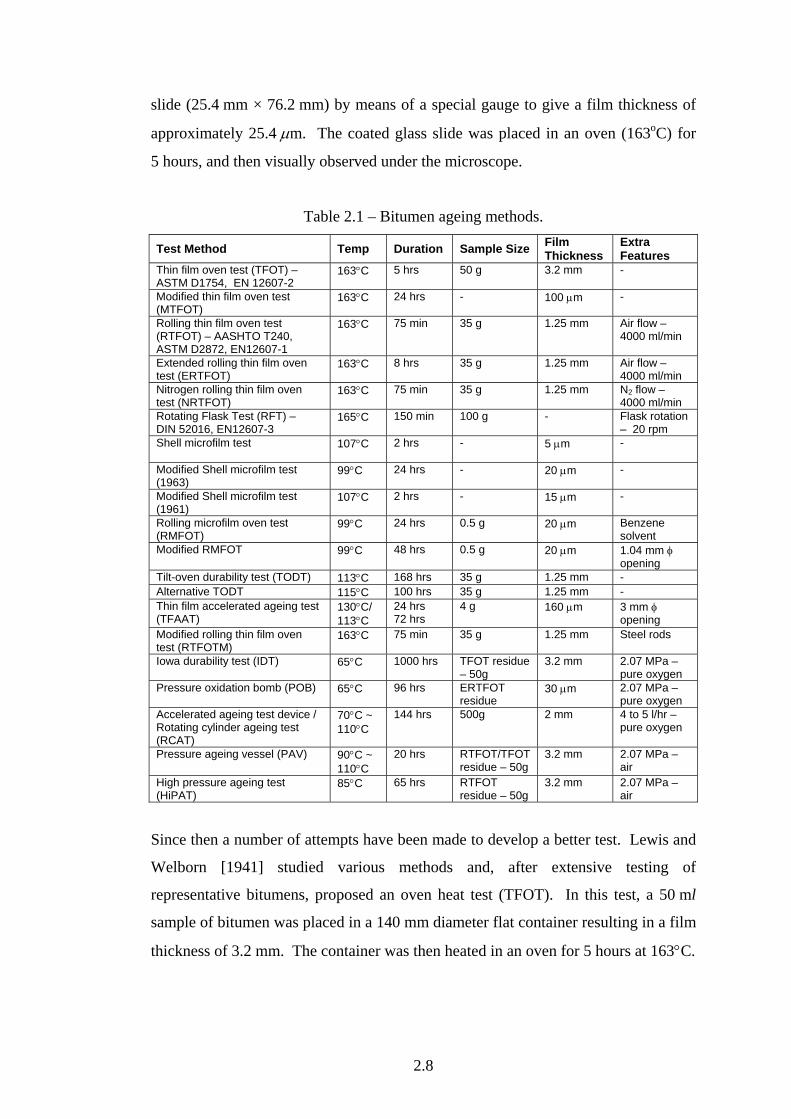
Table 2.1 – Bitumen ageing methods.

Test Method Temp Duration Sample Size Film Thickness

Extra Features

Thin film oven test (TFOT) – ASTM D1754, EN 12607-2

163°C 5 hrs 50 g 3.2 mm -

Modified thin film oven test (MTFOT)

163°C 24 hrs - 100 µm -

Rolling thin film oven test (RTFOT) – AASHTO T240, ASTM D2872, EN12607-1

163°C 75 min 35 g 1.25 mm Air flow – 4000 ml/min

Extended rolling thin film oven test (ERTFOT)

163°C 8 hrs 35 g 1.25 mm Air flow – 4000 ml/min

Nitrogen rolling thin film oven test (NRTFOT)

163°C 75 min 35 g 1.25 mm N2 flow – 4000 ml/min

Rotating Flask Test (RFT) – DIN 52016, EN12607-3

165°C 150 min 100 g - Flask rotation – 20 rpm

Shell microfilm test

107°C 2 hrs - 5 µm -

Modified Shell microfilm test (1963)

99°C 24 hrs - 20 µm -

Modified Shell microfilm test (1961)

107°C 2 hrs - 15 µm -

Rolling microfilm oven test (RMFOT)

99°C 24 hrs 0.5 g 20 µm Benzene solvent

Modified RMFOT 99°C 48 hrs 0.5 g 20 µm 1.04 mm φ opening

Tilt-oven durability test (TODT) 113°C 168 hrs 35 g 1.25 mm - Alternative TODT 115°C 100 hrs 35 g 1.25 mm - Thin film accelerated ageing test (TFAAT)

130°C/ 113°C

24 hrs 72 hrs

4 g 160 µm 3 mm φ opening

Modified rolling thin film oven test (RTFOTM)

163°C 75 min 35 g 1.25 mm Steel rods

Iowa durability test (IDT) 65°C 1000 hrs TFOT residue – 50g

3.2 mm 2.07 MPa – pure oxygen

Pressure oxidation bomb (POB) 65°C 96 hrs ERTFOT residue

30 µm 2.07 MPa – pure oxygen

Accelerated ageing test device / Rotating cylinder ageing test (RCAT)

70°C ~ 110°C

144 hrs 500g 2 mm 4 to 5 l/hr – pure oxygen

Pressure ageing vessel (PAV) 90°C ~ 110°C

20 hrs RTFOT/TFOT residue – 50g

3.2 mm 2.07 MPa – air

High pressure ageing test (HiPAT)

85°C 65 hrs RTFOT residue – 50g

3.2 mm 2.07 MPa – air

Since then a number of attempts have been made to develop a better test. Lewis and

Welborn [1941] studied various methods and, after extensive testing of

representative bitumens, proposed an oven heat test (TFOT). In this test, a 50 ml

sample of bitumen was placed in a 140 mm diameter flat container resulting in a film

thickness of 3.2 mm. The container was then heated in an oven for 5 hours at 163°C.

2.9

The TFOT was adopted by AASHTO in 1959 and ASTM in 1969 [Bell et al., 1994],

as a mean of evaluating the hardening of bitumen during plant mixing. However, a

major concern of the TFOT is the thick binder film. As the bitumen is not agitated

or rotated during the test, there is a concern that ageing (primarily volatile loss) may

be limited to the ‘skin’ of the bitumen sample.

This concern over the testing of bitumen in relatively thick films meant that there

was a move, from the 1950s, to develop or modify ageing tests to age and test

bitumen in microfilm thicknesses. One such example is the modified thin film oven

test (MTFOT), used by Edler et al. [1985], where the binder film was reduced from

3.2 mm to 100 µm with an additional increased exposure time of 24 hours. This

minor modification of the TFOT was done in order to increase the severity of the

ageing process to include oxidative hardening of the binder as well as volatile loss.

Rolling Thin Film Oven Test

The RTFOT is probably the most significant modification of the TFOT involving the

placing of bitumen in a glass jar (bottle) and rotating it in thinner films of bitumen

than that of TFOT. The RTFOT therefore simulates far better the hardening which

bitumen undergoes during asphalt mixing [Hveem et al., 1963; Shell Bitumen

Review, 1973].

The RTFOT was developed by the California Division of Highways and involves

rotating eight glass bottles each containing 35 g of bitumen in a vertically rotating

shelf, while blowing hot air into each sample bottle at its lowest travel position

[Hveem et al., 1963]. During the test, the bitumen flows continuously around the

inner surface of each container in relatively thin films of 1.25 mm at a temperature of

163°C for 75 minutes. The vertical circular carriage rotates at a rate of 15 rpm and

the air flow is set at a rate of 4000 ml/minute. The method ensures that all the

bitumen is exposed to heat and air and the continuous movement ensures that no skin

develops to protect the bitumen. The conditions in the test are not identical to those

found in practice but experience has shown that the amount of hardening in the

RTFOT correlates reasonably well with that observed in a conventional batch mixer

[Whiteoak, 1990].

2.10

Several modifications have also been made to the RTFOT, although most of them

have been relatively minor. For example Edler et al. [1985] used an extended time

period of 8 hours rather than 75 minutes in their extended rolling thin film oven test

(ERTFOT), while Kemp and Predoehl [1981] used 5 hours. A more recent

modification is the development of a nitrogen rolling thin film oven test (NRTFOT)

to determine more accurately the actual loss of volatiles, by minimising oxidative

hardening, during the process [Parmeggiani, 2000]. The procedure is identical to the

standard test except that nitrogen is blown over the exposed surface of the bitumen

samples.

A similar application of the RTFOT with nitrogen gas is the rapid recovery test

(RRT) used to obtain a quantity of ‘recovered binder’ from modified or unmodified

cutback or emulsion binders [MCHW, 1998]. The procedure uses a temperature of

85°C with the RTFOT to evaporate water and/or the light solvent or highly volatile

fraction of emulsions or cutback binders. Nitrogen gas is used instead of air to

minimise oxidative hardening effects.

Rotating Flask Test (DIN 52016)

The RFT method consists of ageing a 100 g sample of bitumen in the flask of a

rotary evaporator for a period of 150 minutes at a temperature of 165°C. As the

flask is rotated at 20 rpm, the material forming the surface of the specimen is

constantly replaced thus preventing the formation of a skin on the surface of the

bitumen [Airey, 2002].

Shell Microfilm Test

The Shell microfilm test is another variation of the principal used with the TFOT. In

this test a very thin, 5 µm, film of bitumen is aged for 2 hours on a glass plate at

107°C [Griffin et al., 1955]. The thinner film thickness was chosen to simulate the

film thicknesses that exist in asphalt mixtures. The bitumen is evaluated on the basis

of viscosity before and after testing to provide the ‘Shell ageing index’. However,

there is limited reported correlation between field performance and laboratory ageing

using the Shell microfilm test [Leslie, 1979], except for the work done on the Zaca-

Wigmore test roads [Zube and Skog, 1969]. Simpson et al. [1959] compared the

2.11

viscosity data for bitumen recovered from the two test roads with the Shell microfilm

test and found a definite correlation between field and laboratory data.

The Shell microfilm test was modified slightly by Hveem et al. [1963] by increasing

the film thickness to 20 µm and the exposure time to 24 hours with a slightly

reduced temperature of 99°C. They also used the residue from RTFOT to prepare

the glass plates (50 mm × 50 mm × 6 mm). These alterations demonstrated an

indirect relationship between field and laboratory hardening. Additionally, slight

variations were made by Traxler [1963] who increased the binder film thickness to

15 µm.

Rolling Microfilm Oven Test

The rolling microfilm oven test (RMFOT) is a modification of the RTFOT in order

to obtain much thinner films of bitumen for ageing [Schmidt and Santucci, 1969].

The test consists of dissolving bitumen in benzene (solvent), coating the inside of the

RTFOT bottles with this solution and then allowing the benzene to evaporate. The

result of this process is the creation of a 20 µm film of bitumen which is then aged at

99°C for 24 hours.

The RMFOT was modified by Schmidt [1973] in order to reduce the amount of

volatile loss during ageing. This was accomplished by placing a capillary in the

opening of the RTFOT bottle and calibrating the capillary size to match the volatile

loss from the bottle to that achieved during the ageing of asphalt mixture specimens

at 60°C. A 1.04 mm diameter opening was selected and in addition the ageing time

was increased from 24 to 48 hours. The modified RMFOT was found to have good

correlation with field cracking of the Zaca-Wigmore pavements as well as with other

field and laboratory aged asphalt mixtures. The notable disadvantage of the test is

that only a very small amount of aged bitumen (0.5 g per bottle) could be produced

for subsequent binder testing.

Tilt-Oven Durability Test

An additional modification of the RTFOT is the California tilt-oven durability test

(TODT) where the oven is tilted 1.06° higher at the front to prevent bitumen

2.12

migrating from the bottles [Kemp and Predoehl, 1981]. In addition the TODT uses a

lower temperature and longer time for ageing compared to the RTFOT, namely

168 hours at 113°C. This level of ageing approximates to that found for pavement

mixtures after 2 years in hot desert climates. In addition, Kemp and Predoehl [1981]

aged laboratory produced specimens in four distinct climates in the field and

concluded that the test results from TODT could be used in a hot climate

specification to control asphalt hardening. McHattie [1983] also performed a

slightly modified TODT with test conditions of 100 hours at 115°C.

Thin Film Accelerated Ageing Test

A modification of the RMFOT is the thin film accelerated ageing test (TFAAT),

developed by Petersen [1989], which has the advantage of producing an increased

amount of aged binder as it uses a sample size of 4 g of binder compared to the 0.5 g

of the RMFOT. Whereas extended heating tests, such as the TFOT and RTFOT,

reflect only the ageing (mainly volatile loss) that occurs during hot-plant mixing, the

TFAAT was developed to produce a representative level of volatilisation and

oxidation to simulate the level of oxidative age hardening typically found for

extended pavement ageing.

The TFAAT was developed to complement a column oxidation procedure developed

by Davis and Petersen [1966] where a 15 µm thick bitumen film, coated on Teflon

particles, was oxidised in a gas chromatographic column at 130°C for 24 hours by

passing air through the column. As the TFAAT uses eight times more binder than

the RMFOT, with subsequent increased binder films, the TFAAT either has to have

longer ageing times or higher test temperatures to achieve the same degree of

oxidative ageing as that found for the RMFOT. Petersen [1989] found that

performing the test at 130°C for 24 hours produced the same degree of oxidative

ageing found for the RMFOT as well as for 11 to 13 year old pavements. As with

the RMFOT, the 31 mm diameter opening for the standard RTFOT bottle was

reduced to 3 mm to restrict excessive volatile loss. The TFAAT can also be

performed at the lower temperature of 113°C but for a longer period of 3 days

compared to the one day test at 130°C.

2.13

Modified Rolling Thin Film Oven Test

One of the main problems with using the RTFOT for modified bitumens is that these

binders, because of their high viscosity, will not roll inside the glass bottles during

the test. In addition, some binders have a tendency to roll out of the bottles. To

overcome these problems, Bahia et al. [1998] developed the Modified Rolling Thin

Film Oven Test (MRTFOT).

The test is identical to the standard RTFOT except that a set of 127 mm long by

6.4 mm diameter steel rods are positioned inside the glass bottles during oven

ageing. The principle is that the steel rods create shearing forces to spread the binder

into thin films, thereby overcoming the problem of ageing high viscosity binders.

Initial trials of the MRTFOT indicate that the rods do not have any significant effect

on the ageing of conventional penetration grade bitumens [Bahia et al., 1998].

However, recent work at the Turner-Fairbanks research centre has indicated that

using the metal rods in the MRTFOT does not solve the problem of roll-out of

modified binder and further validation work is required before the technique can be

accepted [Airey, 2002].

The rapid recovery test (RRT) uses a similar mechanism to MRTFOT to prevent the

roll-out of emulsions or cutback binders but, instead of plain steel rods, the

procedure uses 120 mm long by 12.2 mm diameter stainless steel or PTFE screws

[MCHW, 1998]. The direction of the screw is such that the sample is drawn to the

rear of the bottle during rotation in the RTFOT carousel. Oliver and Tredrea [1997]

also used a roller with a screw thread to age PMBs in the RTFOT where, as the

bottle rotated, the roller ‘screwed’ the binder towards the back wall of the bottle.

Using their modified RTFOT with an exposure time of 9 hours and a temperature of

163°C, Oliver and Tredrea [1997] were able to produce similar changes in the

rheological properties of polymer modified and unmodified bituminous binders to

those found after 2.5 years exposure in a sprayed seal in a hot climate.

2.5.2 Oxidative (Air Blowing) Procedures

Although thin film oven tests can adequately measure the relative hardening

characteristics of bitumens during the mixing process they generally fall short of

2.14

accurately predicting long-term field ageing. Attempts have been made to overcome

this by combining thin film oven ageing with oxidative ageing.

Iowa Durability Test

The Iowa Durability Test (IDT) is one such test that combines thin film ageing with

oxidative ageing [Lee, 1973]. The test consists of ageing binder residue from a

standard TFOT in a pressure vessel at 2.07 MPa using pure oxygen at a temperature

of 65°C for up to 1000 hours. As the residue binder from the TFOT is not

transferred from its container, the film thickness during the pressure-oxidation

treatment is still 3.2 mm. Lee [1973] found that ageing bitumen using the IDT

produced a similar correlation to that found from binders aged in the field over a five

year period. Based on this correlation and a considerable amount of field and

laboratory data, Lee concluded that 46 hours of ageing with the IDT is equivalent to

5 years field ageing in Iowa conditions.

Pressure Oxidation Bomb

Edler et al. [1985] used a similar approach to that used by Lee, where residue from

the ERTFOT was followed by oxidation under pressure using the pressure oxidation

bomb (POB). The POB consists of a cylindrical pressure vessel fitted with a screw-

on cover containing a safety blow-off cap, pressure gauge and stopcock. The vessel

houses a metal support where twelve 40 mm by 40 mm glass plates coated with

30 µm bitumen films are positioned horizontally. The test consists of ageing the

bitumen residue at a pressure of 2.07 MPa at 65°C for 96 hours.

Accelerated Ageing Test Device / Rotating Cylinder Ageing Test

Similar in concept to the RTFOT is the Accelerated Ageing Test Device, also known

as the Rotating Cylinder Ageing Test (RCAT), developed at the Belgian Road

Research Centre (BRRC) [Verhasselt, 2000]. Although standard tests such as the

RTFOT and RFT can adequately simulate construction ageing, their high

temperatures make them unsuitable for simulating field ageing. This has lead to the

development of the accelerated ageing device which has been based on a theoretical

kinetic approach to ageing.

2.15

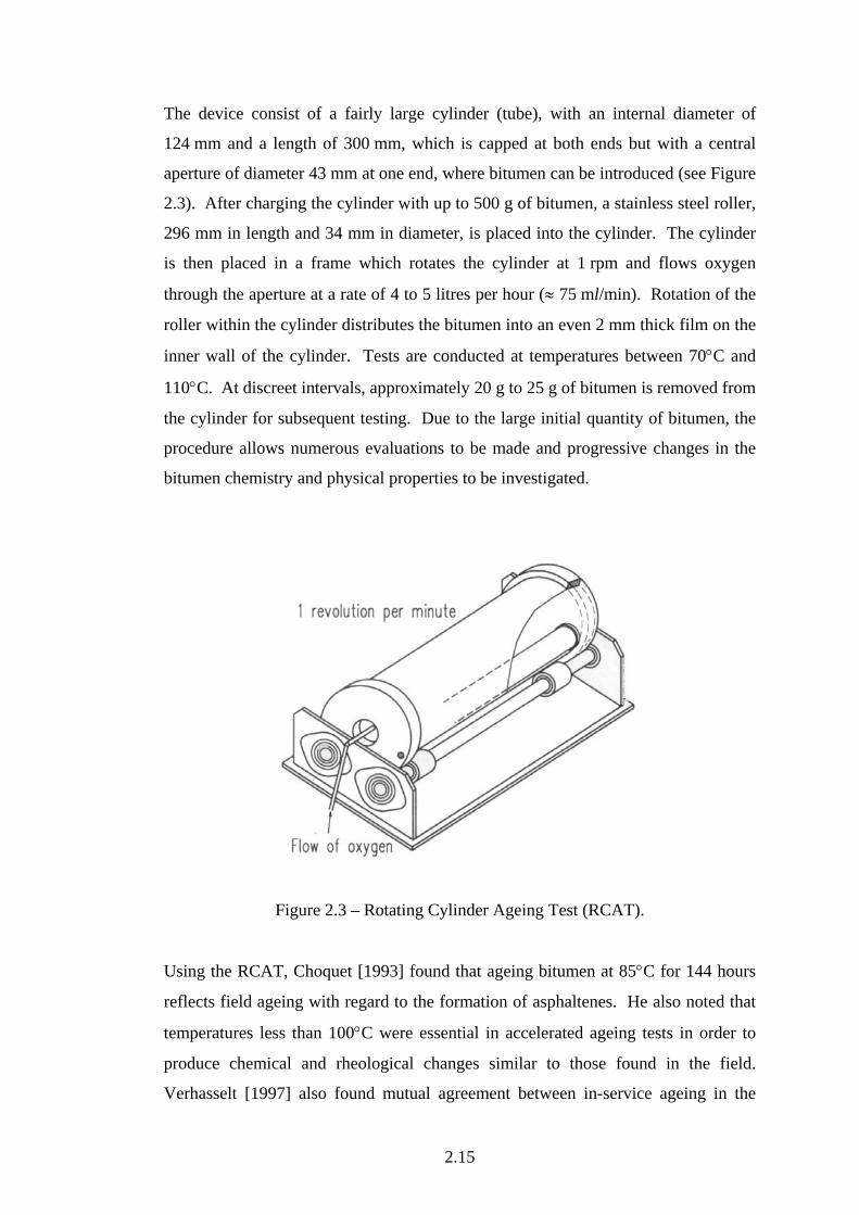
The device consist of a fairly large cylinder (tube), with an internal diameter of

124 mm and a length of 300 mm, which is capped at both ends but with a central

aperture of diameter 43 mm at one end, where bitumen can be introduced (see Figure

2.3). After charging the cylinder with up to 500 g of bitumen, a stainless steel roller,

296 mm in length and 34 mm in diameter, is placed into the cylinder. The cylinder

is then placed in a frame which rotates the cylinder at 1 rpm and flows oxygen

through the aperture at a rate of 4 to 5 litres per hour (≈ 75 ml/min). Rotation of the

roller within the cylinder distributes the bitumen into an even 2 mm thick film on the

inner wall of the cylinder. Tests are conducted at temperatures between 70°C and

110°C. At discreet intervals, approximately 20 g to 25 g of bitumen is removed from

the cylinder for subsequent testing. Due to the large initial quantity of bitumen, the

procedure allows numerous evaluations to be made and progressive changes in the

bitumen chemistry and physical properties to be investigated.

Figure 2.3 – Rotating Cylinder Ageing Test (RCAT).

Using the RCAT, Choquet [1993] found that ageing bitumen at 85°C for 144 hours

reflects field ageing with regard to the formation of asphaltenes. He also noted that

temperatures less than 100°C were essential in accelerated ageing tests in order to

produce chemical and rheological changes similar to those found in the field.

Verhasselt [1997] also found mutual agreement between in-service ageing in the

2.16

field and laboratory ageing using the RCAT for dense mixtures. However Francken

et al. [1997] found that longer ageing times than 240 hours were required to simulate

field ageing (12 years) of porous mixtures.

Pressure Ageing Vessel

The SHRP-A-002A research team developed a method using the pressure ageing

vessel (PAV) to simulate the long-term, in-service oxidative ageing of bitumen in the

field [Kennedy and Harrigan, 1990]. The method involves hardening of bitumen in

the RTFOT followed by an additional oxidation of the residue in the PAV. Although

much of the work done during the SHRP project was with the TFOT, such as the

work done by Christensen and Anderson [1992], the RTFOT was eventually selected

as the recommended procedure [Petersen et al., 1994]. The PAV procedure entails

ageing 50 g of bitumen in a 140 mm diameter pan (to have 3.2 mm of binder film

thickness) in the heated vessel (see Figure 2.4), pressurised with air to 2.07 MPa for

20 hours at temperatures between 90 and 110°C.

Migliori and Corte [1999] investigated the possibility of simulating RTFOT (short-

term ageing) and RTFOT + PAV (long-term ageing) simply by means of PAV

testing for unmodified penetration grade bitumens. They found that 5 hours of PAV

ageing at 100°C and 2.07 MPa was equivalent to standard RTFOT ageing, and that

25 hours of PAV ageing at 100°C and 2.07 MPa was equivalent to standard RTFOT

+ PAV ageing.

High Pressure Ageing Test

The High Pressure Ageing Test (HiPAT) is a modification of the PAV procedure

using a relatively lower temperature of 85°C and a longer duration of 65 hours

[Hayton et al., 1999]. The reason for these modifications was the concern that the

temperatures used in the PAV procedure were unrealistically high compared to

expected pavement temperatures. In addition it was felt, particularly for modified

binders, that the PAV procedure was liable to significantly alter the binders to an

unrepresentative extent compared to that found in the field.

2.17

Figure 2.4 – Pressure Ageing Vessel (PAV).

Initial studies to predict long-term ageing in the field have suggested that the HiPAT

process may be more severe than the natural ageing process for a dense asphalt

mixture, such as Hot Rolled Asphalt (HRA), with a 10 year service life [Hayton et

al., 1999]. However, the severity of this procedure can be useful for an extreme case

study.

2.6 Ageing Tests for Bituminous Mixtures

In addition to artificially ageing binders, a number of methods also exist for

artificially ageing the asphalt mixture. The basic procedure is to artificially age the

mixture and then assess the effect of ageing on key material parameters (e.g.

stiffness, viscosity, strength etc). Extended heating procedures typically expose the

mixture to high temperatures for a specified period(s) of time before suitable testing

(e.g. compressive testing, tests on recovered binder, etc). Oxidation tests typically

utilise a combination of high temperature and pressure oxidation to age specimens.

2.18

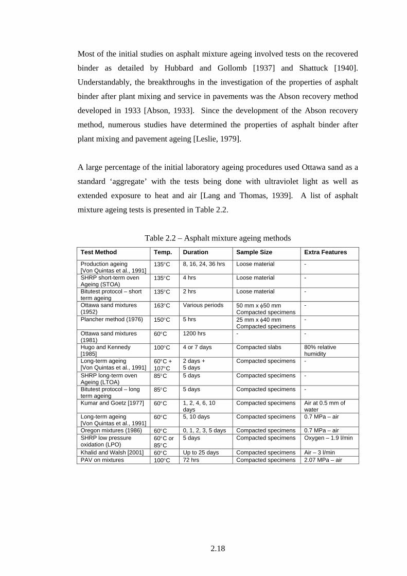
Most of the initial studies on asphalt mixture ageing involved tests on the recovered

binder as detailed by Hubbard and Gollomb [1937] and Shattuck [1940].

Understandably, the breakthroughs in the investigation of the properties of asphalt

binder after plant mixing and service in pavements was the Abson recovery method

developed in 1933 [Abson, 1933]. Since the development of the Abson recovery

method, numerous studies have determined the properties of asphalt binder after

plant mixing and pavement ageing [Leslie, 1979].

A large percentage of the initial laboratory ageing procedures used Ottawa sand as a

standard ‘aggregate’ with the tests being done with ultraviolet light as well as

extended exposure to heat and air [Lang and Thomas, 1939]. A list of asphalt

mixture ageing tests is presented in Table 2.2.

Table 2.2 – Asphalt mixture ageing methods

Test Method Temp. Duration Sample Size Extra Features

Production ageing [Von Quintas et al., 1991]

135°C 8, 16, 24, 36 hrs Loose material -

SHRP short-term oven Ageing (STOA)

135°C 4 hrs Loose material -

Bitutest protocol – short term ageing

135°C 2 hrs Loose material -

Ottawa sand mixtures (1952)

163°C Various periods 50 mm x φ50 mm Compacted specimens

-

Plancher method (1976) 150°C 5 hrs 25 mm x φ40 mm Compacted specimens

-

Ottawa sand mixtures (1981)

60°C 1200 hrs - -

Hugo and Kennedy [1985]

100°C 4 or 7 days Compacted slabs 80% relative humidity

Long-term ageing [Von Quintas et al., 1991]

60°C + 107°C

2 days + 5 days

Compacted specimens -

SHRP long-term oven Ageing (LTOA)

85°C 5 days Compacted specimens -

Bitutest protocol – long term ageing

85°C 5 days Compacted specimens -

Kumar and Goetz [1977] 60°C 1, 2, 4, 6, 10 days

Compacted specimens Air at 0.5 mm of water

Long-term ageing [Von Quintas et al., 1991]

60°C 5, 10 days Compacted specimens 0.7 MPa – air

Oregon mixtures (1986) 60°C 0, 1, 2, 3, 5 days Compacted specimens 0.7 MPa – air SHRP low pressure oxidation (LPO)

60°C or 85°C

5 days Compacted specimens Oxygen – 1.9 l/min

Khalid and Walsh [2001] 60°C Up to 25 days Compacted specimens Air – 3 l/min PAV on mixtures 100°C 72 hrs Compacted specimens 2.07 MPa – air

2.19

2.6.1 Extended Heating Procedures

Pauls and Welborn [1952] exposed 50 mm by 50 mm cylindrical specimens of an

Ottawa sand mixture to 163°C (TFOT and RTFOT ageing temperature) for various

time periods. The compressive strength of the cylinders, as well as the consistency

of the recovered binder, was compared to that of the original (unaged) material.

Results from this study indicated that bitumen recovered from laboratory aged

specimens or aged in the TFOT could be used to assess the short-term hardening

properties of bitumens.

Plancher et al. [1976] used a similar oven ageing procedure to age 25 mm thick by

40 mm diameter specimens at 150°C for 5 hours. Before and after this accelerated

ageing process, the resilient modulus of the samples was measured at 25°C and the

ratio was used as the ageing index.

Hugo and Kennedy [1985] oven aged laboratory compacted slabs at 100°C for 4 or 7

days under either dry atmosphere or 80% relative humidity conditions. After

completion of the ageing process, bitumen was recovered from 10 mm slices off the

top of the slabs. The viscosity of the bitumen before and after the ageing process

was measured and the ratio was used as the ageing index. In addition, the weight

loss of the samples after the ageing process was used to indicate volatile loss.

Most of the methods used for laboratory ageing of asphalt mixtures involve the

ageing of compacted asphalt mixture specimens. However, Von Quintas et al.

[1991] investigated the use of force draft oven ageing to simulate short-term

‘production’ hardening on loose mixture samples. In this method, loose asphalt

material was heated at 135°C in a force draft oven for periods of 8, 16, 24 and 36

hours. Although this method showed similar levels of ageing to those found in the

field, there was considerable scatter in the laboratory data [Bell, 1989].

The SHRP short-term oven ageing (STOA) procedure was developed under the

SHRP-A-003A project, based on the work done by Von Quintas et al. [1991]. The

procedure requires loose mixtures, prior to compaction, to be aged in a forced draft

oven for 4 hours at 135°C. The process was found to represent the ageing occurring

2.20

during mixing and placing and also represents pavements of age less than 2 years

[Bell et al., 1994; Monismith et al., 1994].

Scholz [1995] developed a similar short-term ageing procedure to simulate the

amount of hardening which occurs during the construction process for continuously

graded (DBM) and gap graded (HRA) mixtures. The procedure is similar to the

SHRP STOA procedure except that the conditioning temperature is either 135°C or

the desired compaction temperature, whichever is higher, and the conditioning

period is 2 hours for DBM. However it is also suggested that no conditioning period

is required for HRA mixtures [Brown and Scholz, 2000].

Von Quintas et al. [1991] also investigated long-term ageing using a force draft oven

where compacted asphalt mixture specimens were aged for 2 days at 60°C followed

by an additional 5 days at 107°C. However, Bell [1989] commented that the

elevated temperature level used in the test may cause specimen disruption (structural

loosening) in some cases, particularly for high penetration grade asphalt mixtures

(softer mixtures).

The SHRP long-term oven ageing (LTOA) procedure was also developed under the

SHRP-A-003A project. After STOA, the loose material is compacted and placed in

a forced draft oven at 85°C for 5 days [Harrigan et al., 1994]. The parameters used

for LTOA are meant to represent 7 to 10 years of service. Further field validation

[Bell et al., 1994; Monismith et al., 1994] also suggested the following correlation

between the protocol and field ageing.

• 2 days at 85°C − 2 to 6 years for both Dry-Freeze and Wet-No-Freeze;

• 4 days at 85°C − 7 years for Dry-Freeze and 15 years for Wet-No-Freeze;

• 8 days at 85°C − over 9 years for Dry-Freeze and over 18 years for Wet- No-Freeze climate.

In association with his short-term procedure, Scholz [1995] developed a long-term

oven ageing procedure for the compacted asphalt mixture specimens. The procedure

is identical to the SHRP LTOA procedure consisting of forced draft oven ageing of

2.21

compacted specimens (using short-term aged mixture) at 85°C for 5 days [Brown

and Scholz, 2000].

2.6.2 Oxidative (Air Blowing) Procedures

In addition to oven ageing of loose material and compacted specimens, Von Quintas

et al. [1991] also used a pressure oxidation treatment. The procedure consisted of

conditioning compacted specimens at 60°C at a pressure of 0.7 MPa for 5 or 10 days.

Kim et al. [1986] used a similar pressure oxidation treatment on compacted

specimens of Oregon mixtures. Samples were subjected to oxygen at 60°C and

0.7 MPa for 0, 1, 2, 3 and 5 days. The effects of ageing were evaluated by indirect

tensile stiffness and indirect tensile fatigue. Although the stiffness results generally

increased with ageing, some mixtures showed an initial decrease in stiffness in the

early part of the ageing procedure. This was attributed to a loss of cohesion in the

samples (structural loosening) at the temperature of 60°C used in the ageing test. A

similar phenomenon was observed by Von Quintas et al. [1991] and therefore a

certain level of confinement to the specimen may be applied to keep its structural

integrity as intact as possible during the process.

Another long-term ageing procedure that was developed under the SHRP-A-003A

programme was a Low Pressure Oxidisation (LPO) procedure, carried out on

compacted specimens after they had been short-term aged. The procedure consists

of passing oxygen through a confined triaxial specimen at 1.9 l/min at either 60°C or

85°C for a period of 5 days [Airey, 2002].

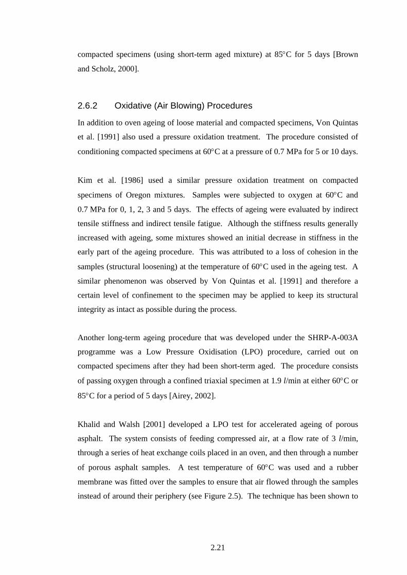
Khalid and Walsh [2001] developed a LPO test for accelerated ageing of porous

asphalt. The system consists of feeding compressed air, at a flow rate of 3 l/min,

through a series of heat exchange coils placed in an oven, and then through a number

of porous asphalt samples. A test temperature of 60°C was used and a rubber

membrane was fitted over the samples to ensure that air flowed through the samples

instead of around their periphery (see Figure 2.5). The technique has been shown to

2.22

recreate the ageing effect produced by the SHRP LTOA procedure, although due to

its lower temperature, longer ageing times are required [Khalid and Walsh, 2000].

Korsgaard et al. [1996] used the PAV to age gyratory compacted dense asphalt

mixture specimens. The binder of the aged specimens was then recovered and

properties were compared to the standard PAV aged binder. They found an ageing

condition of 72 hours at 2.07 MPa and 100°C was comparable to the standard PAV

binder ageing process, but conceded that 60 hours may be more appropriate for more

porous mixtures.

Figure 2.5 – LPO technique for porous asphalt [Khalid and Walsh, 2001]

2.7 Moisture Sensitivity Tests

The development of tests to determine the moisture sensitivity of asphalt mixtures

began in the 1930s [Terrel and Shute, 1989]. Since then numerous tests have been

developed in an attempt to identify the susceptibility of asphalt mixtures to moisture

damage. These moisture sensitivity tests can generally be divided into two

categories:

• Tests conducted on loose coated aggregate; and

• Tests conducted on compacted mixtures.

2.23

Test methods in the first category generally involve immersing the uncompacted

loose mixture in water (or a chemical solution) either at room temperature or an

elevated temperature for a specific period of time, and assessing the separation of the

bitumen binder from the aggregate (stripping) by visual inspection.

Tests on compacted mixtures generally use either samples prepared in the laboratory

or cored from in-service pavements. Typically, the samples are conditioned in water

to simulate in-service conditions and assessment is made by a ratio of conditioned to

unconditioned mechanical properties of the material (i.e. strength or stiffness).

Immersion trafficking tests which incorporate traffic loading during a moisture

conditioning process are not considered in this review.

2.7.1 Tests on Loose Mixtures

Several methods have been developed to assess the amount of bitumen loss which

occurs as a result of uncompacted, coated aggregate being immersed in water.

However, for the majority of these tests little information is available to correlate test

data with field performance. The various methods differ in the type of specimen

used, the way in which the specimen is immersed in water and the manner in which

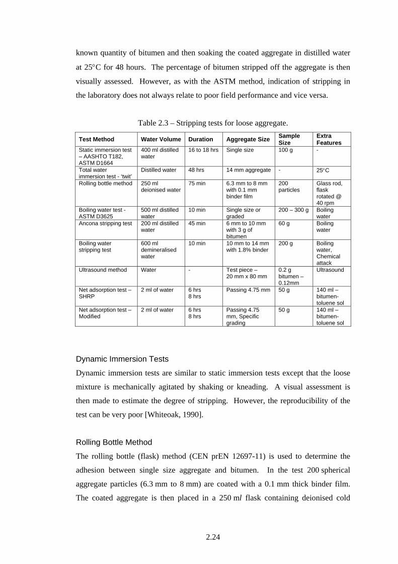
stripping (adhesion loss) is assessed. A list of stripping tests for loose aggregates is

presented in Table 2.3.

Static Immersion Tests

The static immersion test [AASHTO T182, ASTM D1664] involves coating 100 g of

aggregate with bitumen, immersing it for 16 to 18 hours in 400 ml of distilled water

(pH 6 to 7), then visually estimating the total visible area of the coated aggregate as

above or below 95%. The visual assessment is made while the mixture is still

immersed in the water. Although the method may indicate mixtures showing some

degree of moisture sensitivity, it is doubtful that the long-term potential of stripping

is considered [Terrel and Shute, 1989]. The static immersion test was also

discontinued as an ASTM standard in 1993 [Airey, 2002].

Another example of a static immersion test is the total water immersion test (‘twit’

test) [Whiteoak, 1990]. The test involves coating 14 mm single size aggregate with a

2.24

known quantity of bitumen and then soaking the coated aggregate in distilled water

at 25°C for 48 hours. The percentage of bitumen stripped off the aggregate is then

visually assessed. However, as with the ASTM method, indication of stripping in

the laboratory does not always relate to poor field performance and vice versa.

Table 2.3 – Stripping tests for loose aggregate.

Test Method Water Volume Duration Aggregate Size Sample Size

Extra Features

Static immersion test – AASHTO T182, ASTM D1664

400 ml distilled water

16 to 18 hrs Single size 100 g -

Total water immersion test - ‘twit’

Distilled water 48 hrs 14 mm aggregate - 25°C

Rolling bottle method 250 ml deionised water

75 min 6.3 mm to 8 mm with 0.1 mm binder film

200 particles

Glass rod, flask rotated @ 40 rpm

Boiling water test - ASTM D3625

500 ml distilled water

10 min Single size or graded

200 – 300 g Boiling water

Ancona stripping test 200 ml distilled water

45 min 6 mm to 10 mm with 3 g of bitumen

60 g Boiling water

Boiling water stripping test

600 ml demineralised water

10 min 10 mm to 14 mm with 1.8% binder

200 g Boiling water, Chemical attack

Ultrasound method Water - Test piece – 20 mm x 80 mm

0.2 g bitumen – 0.12mm

Ultrasound

Net adsorption test – SHRP

2 ml of water 6 hrs 8 hrs

Passing 4.75 mm 50 g 140 ml – bitumen-toluene sol

Net adsorption test – Modified

2 ml of water 6 hrs 8 hrs

Passing 4.75 mm, Specific grading

50 g 140 ml – bitumen-toluene sol

Dynamic Immersion Tests

Dynamic immersion tests are similar to static immersion tests except that the loose

mixture is mechanically agitated by shaking or kneading. A visual assessment is

then made to estimate the degree of stripping. However, the reproducibility of the

test can be very poor [Whiteoak, 1990].

Rolling Bottle Method

The rolling bottle (flask) method (CEN prEN 12697-11) is used to determine the

adhesion between single size aggregate and bitumen. In the test 200 spherical

aggregate particles (6.3 mm to 8 mm) are coated with a 0.1 mm thick binder film.

The coated aggregate is then placed in a 250 ml flask containing deionised cold

2.25

water and a glass rod and rotated at 40 rpm for three days. The amount of retained

bitumen is then visually determined [Airey, 2002].

Boiling Water Test (ASTM D3625)

This test is a result of the assimilation of different boiling tests used by several US

state agencies [Terrel and Shute, 1989], such as the Texas boiling test [Kennedy et

al., 1983]. The boiling water test involves placing a 200 to 300 g sample of coated

aggregate (single size aggregate or aggregate graded to design specifications) in

boiling water (500 ml of distilled water) for 10 minutes. The mixture is stirred three

times with a glass rod whilst it is being boiled. After boiling, the mixture is dried

and the amount of bitumen loss is determined by visual assessment. The test is very

subjective and known to provide inconsistent results in terms of identifying moisture

sensitive mixtures. In addition the test only reflects the loss of adhesion and does not

address loss of cohesion.

Ancona Stripping Test

The Ancona Stripping Test (AST) is used to evaluate the stripping potential of a

bitumen-aggregate system [Bocci and Colagrande, 1993]. The procedure entails

placing a sample of bituminous gravel (60 g of gravel, passing 10 mm sieve and

retained on 6 mm sieve, mixed with 3 g of bitumen) in a 600 ml beaker with 200 ml

of distilled water. The 600 ml beaker is then placed in a 2000 ml beaker containing

600 ml of boiling water for 45 minutes. At the end of this period, the beaker is

removed and cooled to ambient temperature. The bituminous gravel is removed

from the beaker and a visual assessment made of the percentage stripping.

Boiling Water Stripping Test

The BRRC have combined the boiling water test with a more objective means of

assessing the amount of stripping using a stripping ratio calibration curve, thereby

eliminating the low precision associated with visual assessment [Choquet and

Verhasselt, 1993]. The procedure involves coating 1.5 kg of aggregate (10 to 14 mm

fraction) with 1.8% by mass of bitumen [BRRC, 1991]. Mixtures of uncoated (bare)

aggregate and the coated aggregate are then produced and subjected to chemical

attack to produce a calibration curve of acid consumption against percentage

uncoated aggregate. 200 g of the coated aggregate is then boiled in 600 ml of

2.26

demineralised water for 10 minutes, allowed to dry and subjected to chemical attack

to determine, based on the calibration curve, the amount of stripping.

Ultrasonic Method

Vuorinen and Valtonen [1999] developed an ultrasonic method to measure the

resistance to stripping of coated aggregates. In the test a polished stone test piece

(20 mm × 80 mm, with a thickness of 10 mm) is coated with 0.2 g of bitumen to give

a binder film thickness of 0.12 mm. The coated test piece is then subjected to

ultrasound under water where microscopically small bubbles of negative pressure

strip the bitumen mechanically from the stone. The degree of stripping is determined

either by weighing the stripped test piece or by visual assessment.

Net Adsorption Test

The Net Adsorption Test [SHRP Designation M-001; Harrigan et al., 1994] was

developed by Curtis et al. [1993] and used as a screening procedure for selecting

bitumens and aggregates, as well as determining the effectiveness of antistripping

additives, as part of the Superpave Mixture Design Method [Kennedy et al., 1994].

This is accomplished by measuring the amount of bitumen dissolved in toluene that

is adsorped onto the aggregate surface followed by the amount which is desorped

(removed) by the addition of water to the system. The amount of bitumen which

remains on the aggregate after aqueous desorption is termed the Net Adsorption.

The adsorption value over 70% is considered as a good aggregates-binder bond

performance [Cominsky, 1994].

Walsh et al. [1996] later proposed a modification to the Net Adsorption Test. In the

modified net adsorption test, the aggregate is prepared to a specific grading rather

than simply passing the 4.75 mm sieve. In addition an initial adsorption value is

calculated as well as the net adsorption in order to provide a more discriminating

assessment of affinity and resistance to stripping of the binder-aggregate system

[Woodside et al., 1994].

2.27

2.7.2 Tests on Compacted Mixtures

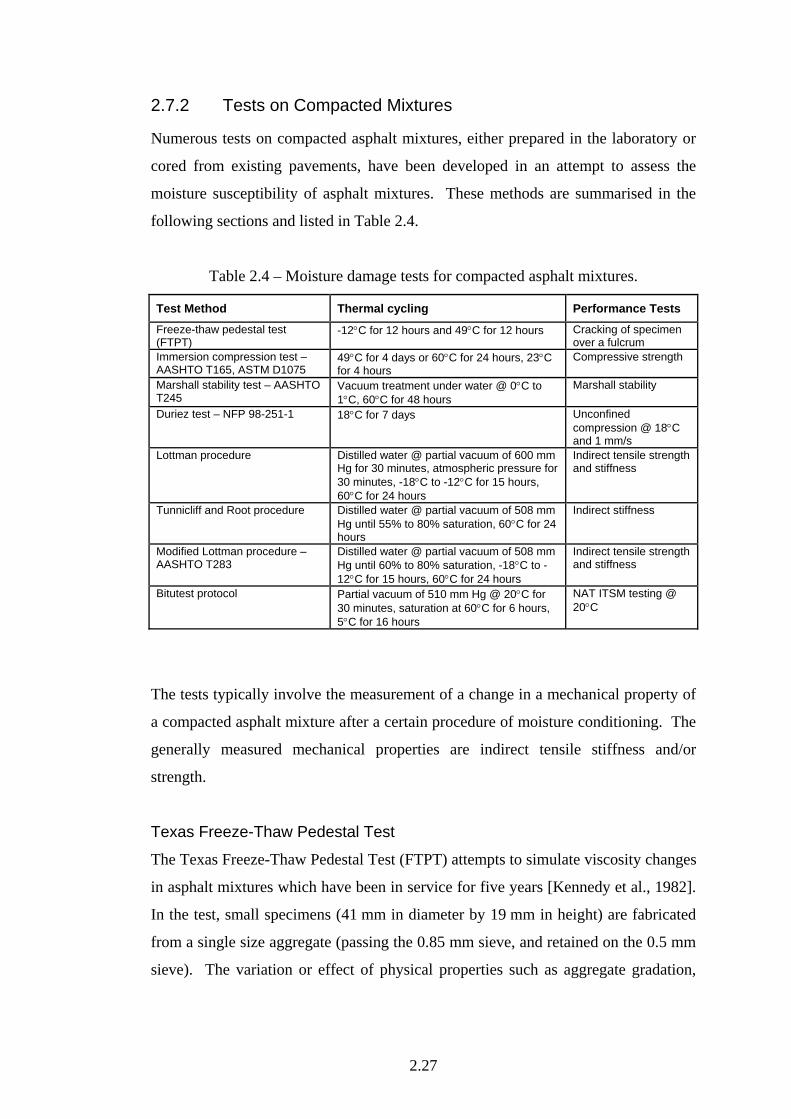
Numerous tests on compacted asphalt mixtures, either prepared in the laboratory or

cored from existing pavements, have been developed in an attempt to assess the

moisture susceptibility of asphalt mixtures. These methods are summarised in the

following sections and listed in Table 2.4.

Table 2.4 – Moisture damage tests for compacted asphalt mixtures.

Test Method Thermal cycling Performance Tests

Freeze-thaw pedestal test (FTPT)

-12°C for 12 hours and 49°C for 12 hours Cracking of specimen over a fulcrum

Immersion compression test – AASHTO T165, ASTM D1075

49°C for 4 days or 60°C for 24 hours, 23°C for 4 hours

Compressive strength

Marshall stability test – AASHTO T245

Vacuum treatment under water @ 0°C to 1°C, 60°C for 48 hours

Marshall stability

Duriez test – NFP 98-251-1 18°C for 7 days Unconfined compression @ 18°C and 1 mm/s

Lottman procedure Distilled water @ partial vacuum of 600 mm Hg for 30 minutes, atmospheric pressure for 30 minutes, -18°C to -12°C for 15 hours, 60°C for 24 hours

Indirect tensile strength and stiffness

Tunnicliff and Root procedure Distilled water @ partial vacuum of 508 mm Hg until 55% to 80% saturation, 60°C for 24 hours

Indirect stiffness

Modified Lottman procedure – AASHTO T283

Distilled water @ partial vacuum of 508 mm Hg until 60% to 80% saturation, -18°C to -12°C for 15 hours, 60°C for 24 hours

Indirect tensile strength and stiffness

Bitutest protocol Partial vacuum of 510 mm Hg @ 20°C for 30 minutes, saturation at 60°C for 6 hours, 5°C for 16 hours

NAT ITSM testing @ 20°C

The tests typically involve the measurement of a change in a mechanical property of

a compacted asphalt mixture after a certain procedure of moisture conditioning. The

generally measured mechanical properties are indirect tensile stiffness and/or

strength.

Texas Freeze-Thaw Pedestal Test

The Texas Freeze-Thaw Pedestal Test (FTPT) attempts to simulate viscosity changes

in asphalt mixtures which have been in service for five years [Kennedy et al., 1982].

In the test, small specimens (41 mm in diameter by 19 mm in height) are fabricated

from a single size aggregate (passing the 0.85 mm sieve, and retained on the 0.5 mm

sieve). The variation or effect of physical properties such as aggregate gradation,

2.28

density, aggregate interlock are minimised through the use of a single size aggregate

so that the test primarily evaluates the strength of bonding and binder cohesion.

After fabrication, the specimen is cured at 23°C for 3 days then placed on a pedestal

which acts as a fulcrum. The arrangement is placed in a water bottle and subjected

to thermal cycling, consisting of freezing at -12°C for 12 hours and thawing at 49°C

for 12 hours (total 24 hours), until the specimen is cracked. Kennedy et al. [1982]

proposed that the range of values between 10 and 20 thermal cycles to cracking

would be the borderline between stripping and non-stripping mixtures. The test

seems to be able to identify some moisture susceptible mixtures while being

insensitive to others.

Immersion Compression Test

The Immersion Compression Test [AASHTO T165, ASTM D1075] is widely used

throughout the United States to evaluate the loss of strength of compacted asphalt

mixtures. In the test the index of retained strength (IRS) is obtained by comparing

the compressive strength of unconditioned specimens (air cured at 23°C for 4 hours)

to that of conditioned duplicate specimens which have been immersed in water for

4 days at 49°C (or 60°C for 24 hours) and then conditioned in water at 23°C for

4 hours. The Asphalt Institute recommends that mixtures be rejected if they have an

IRS less than or equal to 75% [Terrel and Shute, 1989].

Marshall Stability Test

The Marshall Stability Test [AASHTO T245] is widely used to evaluate the relative

performance of asphalt mixtures. In the test, the stability of unconditioned

specimens is compared with the stability of duplicate specimens which have been

subjected to some form of moisture conditioning. Terrel and Shute [1989] note that

the conditioning procedure varies amongst organisations and is usually an adaptation

from one of the existing procedures.

The Shell method uses at least eight specimens manufactured using a prescribed

aggregate type, aggregate gradation, bitumen content and void content [Whiteoak,

1990]. Four of these specimens are tested according to the standard Marshall

2.29

stability. The remaining four specimens are vacuum treated under water at a

temperature between 0 and 1°C, stored in a water bath at 60°C for 48 hours and

tested for Marshall stability. The retained Marshall stability is then determined as

the ratio of the conditioned/unconditioned specimens.

Duriez Test (NFP 98-251-1)

The Duriez test has been used for over 40 years in France to assess moisture

sensitivity of asphalt mixtures [Corte and Serfass, 2000]. The procedure is

performed on 80 mm or 120 mm diameter cylindrical specimens, statically

compacted under a pressure of 12 MPa. The moisture conditioning consists of

submerging specimens under water at 18°C for 7 days. The sensitivity to moisture is

then assessed as the ratio of the unconfined compressive strength of the conditioned

to unconditioned specimens at a temperature of 18°C and a loading rate of 1 mm/s.

Lottman Procedure

The Lottman procedure [Lottman, 1982] is commonly used to predict moisture

damage in dense-graded bituminous mixtures. In this procedure samples are

subjected to vacuum saturation alone or vacuum saturation followed by freeze-plus-

warm-water soak, more commonly referred to as freeze-thaw. The test specimens,

100 mm in diameter and 63 mm in height, are then tested to produce conditioned to

unconditioned ratios of indirect tensile strength and stiffness. The short-term

analysis, vacuum saturated to dry ratio, is intended to reflect a field performance up

to 4 years, while the long-term performance, vacuum saturated plus freeze-thaw to

dry ratio estimates the field performance from 3 to 12 years.

The vacuum saturation part of the procedure consists of submerging the specimens in

distilled water in a partial vacuum of 600 mmHg (80 kPa) for 30 minutes. The

samples are then left saturated at atmospheric pressure for a further 30 minutes,

conditioned in water at the test temperature for 3 hours and then tested to obtain

conditioned and unconditioned ratios of indirect tensile strength and stiffness. The

freeze-thaw procedure consists of tightly wrapping the vacuum saturated specimens

in plastic wrap, placing them in heavy-duty plastic bags, each containing

approximately 3 ml of distilled water, and freezing them at –18 to –12°C for

2.30

15 hours. The plastic wrap is then removed and the samples are heated to 60°C in a

distilled water bath for 24 hours, conditioned in water at the test temperature for

3 hours and tested.

Tunnicliff and Root Procedure

The Tunnicliff and Root procedure [Tunnicliff and Root, 1984] is similar to the

Lottman procedure [Lottman, 1982]. However the procedure uses a slightly

different vacuum saturation and thermal treatment methodology, and excludes

freezing of the saturated specimens. The procedure controls the degree of saturation

to ensure that enough moisture is present to initiate moisture damage and to avoid

unrelated damage, such as stresses induced from over saturation. Conditioning

involves submerging the specimens in distilled water and incrementally applying a

partial vacuum of 508 mmHg (68 kPa) in 5 minute increments until a degree of

saturation between 55 to 80% is achieved. The specimens are then heated in a

distilled water bath at 60°C for 24 hours, conditioned in water at the test temperature

of 25°C for 1 hour and tested.

Modified Lottman Procedure (AASHTO T283)

The AASHTO T283 (or modified Lottman) procedure combines features of both the

Lottman [1982] and Tunnicliff and Root [1984] procedures. The Lottman procedure

attempts to achieve a 100% saturation in its specimens, while the Tunnicliff and

Root procedure attempts to control the saturation level between 55 and 80%. Due to

concerns on over saturation, where the negative pressure applied in the vacuuming

process may cause extra non-moisture-related damage in specimens, the modified

Lottman procedure uses a decreased saturation level of between 60 and 80%

[Scherocman et al., 1986]. As the saturation level achieved by partial vacuum is

primarily responsive to the magnitude of the vacuum and relatively independent of

the length of time, this reduced saturation was achieved by reducing the partial

vacuum from 600 mmHg (80 kPa) to 508 mmHg (68 kPa).

LINK Bitutest Moisture Sensitivity Protocol

Scholz [1995] produced a test method for measuring moisture sensitivity of

compacted bituminous mixtures that involves determining the ratio of conditioned to

2.31

unconditioned indirect stiffness modulus values as measured with the Nottingham

Asphalt Tester (NAT). The conditioning consists of saturation under a partial

vacuum of 510 mmHg (68 kPa) at 20°C for 30 minutes, followed by immersion in

water at 60°C for 6 hours, and immersion in water at 5°C for 16 hours. The samples

are finally conditioned in water at 20°C for 2 hours prior to the stiffness

measurement.

A very severe form of winter conditioning has been produced by Hobeda [2000] for

extreme Nordic conditions. The procedure consists of submerging test specimens

under vacuum saturation, firstly, in a concentrated NaCl solution for 48 hours and

then in a distilled water environment for a further 48 hours. The specimens are then

subjected to seven freeze-thaw cycles (-20°C and 20°C for 12 hours each) before

indirect tensile stiffness testing at 10°C.

2.8 Summary and Conclusions

An extensive review of existing test methods, protocols and techniques for the

assessment of ageing and moisture sensitivity of bituminous materials, has been

undertaken. The testing methods can be broadly grouped into the following

categories; 1) Binder ageing, 2) Mixture ageing (loose mixture or compacted

specimen) and 3) Moisture sensitivity (loose mixture or compacted specimen).

The binder ageing can be divided into short and long term ageing. The ‘short-term’

describes the ageing process (mainly volatile loss) that occurs during the asphalt

mixture construction process (heating up, mixing, delivery and compaction) and the

‘long-term’ describes the progressive oxidation process of the in-place material in

the field during its service life.

The most commonly used binder ageing tests are the high temperature TFOT and

RTFOT. It is noted that bitumen aged in the TFOT and RTFOT experiences higher

volatile loss during testing compared to that experienced during low temperature

field ageing of pavement mixtures. Also the level of oxidative ageing in the tests is

considerably lower than that found during field ageing. Therefore these tests are

2.32

only suitable to simulate for short-term ageing, but not ideal to estimate the long-

term ageing of bitumen in pavements.

Based on the inability of these high temperature oven ageing tests to predict ‘long-

term’ field ageing, tests such as the Shell Microfilm Test, RMFOT, TFAAT and

others were introduced with reduced temperatures and increased ageing times. Tests

such as POB and PAV utilise a pressurised condition to the ageing process to give a

more accelerated oxidisation process under moderate temperatures and relatively

short test periods. From the questionnaire survey undertaken (see Appendix B), the

most commonly used tests for short-term ageing and long-term ageing simulation

appear to be the RTFOT and PAV protocols respectively.

Eckmann [1999] stated that RTFOT and similar test methods are probably adequate

for short-term ageing as there is good evidence that they simulate short-term ageing

reasonably well. Nevertheless he admitted that these test methods may need to

overcome some operational difficulties when testing PMBs, such as the use of the

MRTFOT as recommended by Bahia et al. [1998]. In terms of long-term ageing,

Eckmann proposed to look into the kinetic aspect of ageing, such as the RCAT,

although he generally concluded that no one test seems to be satisfactory in all cases.

Regardless of the short-term or long-term aspect, the elevated temperature is

apparently the essential and critical acceleration factor for ageing process. However,

for the long-term aspect, there are concerns over this ‘unrealistically’ elevated

temperature as it could significantly alter the binders to an unrepresentative extent to

that found in the field, particularly for modified binders [Hayton et al., 1999]. Thus

the introduction of a pressurised condition, such as the PAV protocol, seems to be a

breakthrough approach as it gives one more factor to control the acceleration of the

ageing process (oxidisation) together with the temperature and test duration. The

HiPAT procedure seems to be a reasonable and recommendable protocol for the

long-term ageing simulation as it uses an even lower temperature than the PAV.

Most ageing protocols for the asphalt mixture also use an elevated temperature as a

dominant factor to age the binder (in the mixture) in an accelerated manner to

shorten the test period. It is interesting to note that the elevated temperatures applied

2.33

on the compacted mixture are considerably lower than those for the loose mixture.

This is to avoid/minimise unnecessary structural disruption (due to cohesion loss of

binder) caused by the high temperature. The ‘highest’ temperature applied on

compacted specimens was found to be 100oC used by Korsgaard et al. [1996] for

their PAV trial. However, this was to recover binder from the specimens, rather than

performing any mechanical test on the compacted specimen. Knowing that even at

60oC there were concerns over the high temperature effect [Kim et al., 1986; Von

Quintas et al., 1991 and Bell, 1989], 85oC appears to be the maximum applicable

temperature for compacted specimens.

Moisture susceptibility tests generally have a conditioning and an evaluation phase.

The conditioning processes associated with most test methods are to simulate the

deterioration of the asphalt mixture in the field exposure conditions, in an

accelerated manner to be tested in a reasonably short period of time. Normally the

acceleration is achieved by immersing the material at an elevated temperature. It is

noted that the elevated temperature applied on the loose mixture is commonly the

boiling temperature of 100oC. However, 60oC appears to be the highest temperature

used on compacted specimens. As with the ageing tests, this is to avoid (or

minimise) any unnecessary structural disruption caused by the high temperature,

rather than moisture damage. Additionally the samples can be subjected to extra

conditioning factors which do not necessarily simulate field conditions but possibly

more accelerate the moisture damage, such as ultrasonic methods [Vuorinen and

Valtonen, 1999].

The two general methods of evaluating ‘conditioned’ specimens are either a visual

evaluation or the subjection of the specimen to a physical test. Visual evaluation is

used extensively in moisture susceptibility procedures especially for the coated

aggregate tests (uncompacted ‘loose’ mixture). However, visual assessment tends to

be rather subjective and moreover, the assessment is performed on the material

‘before’ its compaction process, which is one of the most decisive factors for the

‘field performance’ of the material.

Most moisture sensitivity test procedures on the compacted mixture measure the loss

of strength or stiffness of an asphalt mixture due to moisture damage. The most

2.34

common way of quantifying the damage caused by the conditioning process is to

directly compare the ‘conditioned’ mechanical properties to those of

‘unconditioned’. The mechanical properties can be evaluated using various

mechanical tests which can be divided into destructive (compression, stability,

indirect tensile strength and fatigue) and non-destructive (indirect tensile stiffness

and resilient modulus) approaches. An apparent advantage of using a non-

destructive test is that the very same specimen can be used for a direct comparison of

unconditioned and conditioned properties. Therefore a relatively small number of

specimens is required to define a trend.

Saturation is a common link to all the conditioning procedures and is the key to the

laboratory simulation of moisture damage in the test specimens. Saturation is

obtained either by immersion of the specimen in static or boiling water and/or by

applying a certain degree of vacuum. The principal reason for the vacuum is to draw

the water into the specimen to shorten the time required for the specimen to reach the

desired saturation level.

The correlation of ageing simulated in the laboratory test and that of the field

material has been relatively well established, compared to the correlation of moisture

sensitivity tests to field performance. Since ageing is only focussed on the binder

property, the correlation can be directly established by comparing the chemical

component and/or physical properties of the binder aged in the laboratory to those of

the binder recovered from field material of a known period of service life and in a

known climate condition. However, moisture sensitivity is focussed on mixture

properties which are a much more complicated aspect. In field material after a

certain period of service life, the measured material properties result from combined

effects of various damage factors, such as binder ageing, together with adhesion loss

due to moisture damage, while the mixtures (including aggregates) are gradually

degraded by traffic load and/or other environmental factors. Thus, it is practically

difficult to directly correlate the material property change (strength, stiffness etc)

from a moisture sensitivity test to those observed in field material, in terms of

service life.

2.35

It is interesting to note that existing durability protocols are designed to investigate

one aspect only (i.e. ageing test for ageing sensitivity, moisture sensitivity test for

moisture damage). However, particularly in the long-term service condition, it is

more likely that the pavement is undergoing both aspects of ageing and moisture

damage together (i.e. materials are damaged by water infiltration while the binder in

the material is being aged).

3.1

Chapter 3. Preliminary Trials

3.1 Ageing & Moisture Sensitivity Test Review

From the literature review (see Chapter 2) and the questionnaire survey undertaken

(see Appendix B), considering both practicability and the availability of testing

equipment in the laboratory, a couple of different ageing regimes and a moisture

sensitivity regime were selected as the first step of the test programme.

The main purpose of these preliminary trials was to find a suitable test method which

could reproduce in the laboratory the decrease in stiffness modulus that had been

measured from the HMB trial site (see Section 1.1). For the purpose of combining

ageing and moisture sensitivity process, this preliminary investigation basically

performed the ageing process first, followed by the water sensitivity process. This

was considered to be a combined durability protocol at this stage.

A 28 mm Dense Bitumen Macadam (DBM) base material [BS 4987: Part 1, 2001]

using a typical acidic aggregate (referred to as Acidic) and a 15 Penetration grade of

binder (referred to as 15B, 4% by mass) was used to replicate the material used in

the HMB trial site. A target air void content of 8% was identified (this was the

typical air void content measured from the site) based on 'Rice' maximum density of

the mixture [BSEN 12697: Part 5, 2002] and 'sealed' bulk density of core specimens

(see Chapter 5 for more details of the specimen production). The mixture was

compacted using a laboratory roller compactor and cylindrical specimens were cored

from the slab for standard Indirect Tensile Stiffness Modulus (ITSM) testing [BS DD

213, 1993]. The Stiffness Modulus of the material at 20oC was the main

performance parameter used throughout this study.

The stiffness modulus was measured before and after each ageing regime.

Following each ageing regime a moisture sensitivity cycle was performed on the

same specimens and the stiffness modulus was again measured. The LINK moisture

sensitivity protocol [Scholz, 1995] was selected for the standard moisture sensitivity

test at this stage. Each cycle consisted of conditioning the specimen in water, at

3.2

60oC for 6 hours, 5oC for 16 hours and finally 20oC for 2 hours. Typically, each test

comprised up to four moisture conditioning cycles. The following sub-sections

describe the selected regimes in more detail.

Regime #1

Regime #1 was used as the control. Specimens were stored at 5oC in a cold dry

room in an attempt to prevent any ageing or moisture damage.

Regime #2

Regime #2 used the standard LINK ageing protocol where the compacted specimen

was heated in a dry oven at 85oC for 120 hours [Scholz, 1995].

Regime #3

Regime #3 was similar to regime #2 but included a large water bath placed in the

oven to create a relatively humid environment for the ageing process in an attempt to

combine the effects of ageing and moisture damage.

Regime #4

Regime #4 used a Low Pressure Oxidation (LPO) configuration where hot air at

85oC was forced through the specimen using a vacuum pump. The test temperature

was selected to be 85oC to give the same temperature condition as in the other

regimes. This was achieved by placing the specimen unit (see Figure 3.1) into a dry

oven at 85oC. The flow rate was 3l/min, based on a configuration developed by

Khalid and Walsh [2001], and the test duration was 120 hours (identical to

Regimes #2 and #3). The LPO configuration was used to ensure continued oxidation

throughout the entire specimen during the test duration.

Regime #5

Regime #5 used the standard Pressure Ageing Vessel (PAV) for binder ageing to age

the compacted mixture specimens. The HiPAT protocol [Hayton et al., 1999] was

used, where a temperature of 85oC and a pressure of 2.1 MPa were applied for

65 hours. The HiPAT protocol was chosen as it uses a relatively lower temperature,

which appears to be more applicable to the compacted specimen from the literature

review (see Section 2.5.2), than the standard PAV protocol. A purpose built tray was

used to place two specimens into the vessel.

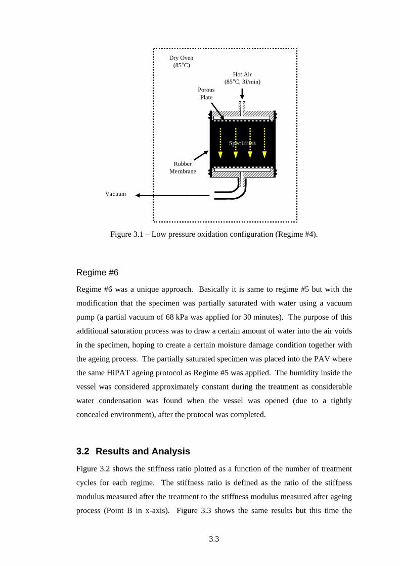
3.3

Specimen

Hot Air(85oC, 3l/min)

RubberMembrane

Va c uum

PorousPlate

Dry Oven(85oC)

Figure 3.1 – Low pressure oxidation configuration (Regime #4).

Regime #6

Regime #6 was a unique approach. Basically it is same to regime #5 but with the

modification that the specimen was partially saturated with water using a vacuum

pump (a partial vacuum of 68 kPa was applied for 30 minutes). The purpose of this

additional saturation process was to draw a certain amount of water into the air voids

in the specimen, hoping to create a certain moisture damage condition together with

the ageing process. The partially saturated specimen was placed into the PAV where

the same HiPAT ageing protocol as Regime #5 was applied. The humidity inside the

vessel was considered approximately constant during the treatment as considerable

water condensation was found when the vessel was opened (due to a tightly

concealed environment), after the protocol was completed.

3.2 Results and Analysis

Figure 3.2 shows the stiffness ratio plotted as a function of the number of treatment

cycles for each regime. The stiffness ratio is defined as the ratio of the stiffness

modulus measured after the treatment to the stiffness modulus measured after ageing

process (Point B in x-axis). Figure 3.3 shows the same results but this time the

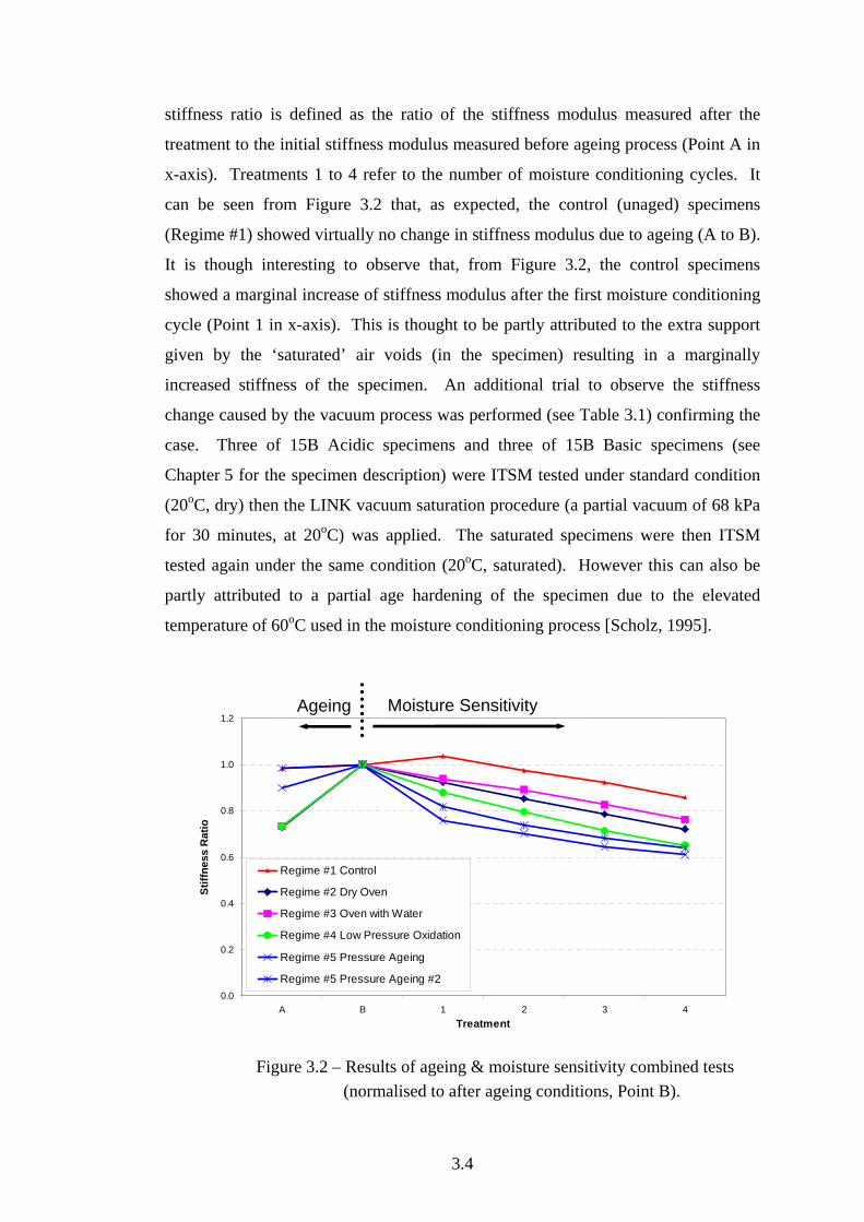
3.4

stiffness ratio is defined as the ratio of the stiffness modulus measured after the

treatment to the initial stiffness modulus measured before ageing process (Point A in

x-axis). Treatments 1 to 4 refer to the number of moisture conditioning cycles. It

can be seen from Figure 3.2 that, as expected, the control (unaged) specimens

(Regime #1) showed virtually no change in stiffness modulus due to ageing (A to B).

It is though interesting to observe that, from Figure 3.2, the control specimens

showed a marginal increase of stiffness modulus after the first moisture conditioning

cycle (Point 1 in x-axis). This is thought to be partly attributed to the extra support

given by the ‘saturated’ air voids (in the specimen) resulting in a marginally

increased stiffness of the specimen. An additional trial to observe the stiffness

change caused by the vacuum process was performed (see Table 3.1) confirming the

case. Three of 15B Acidic specimens and three of 15B Basic specimens (see

Chapter 5 for the specimen description) were ITSM tested under standard condition

(20oC, dry) then the LINK vacuum saturation procedure (a partial vacuum of 68 kPa

for 30 minutes, at 20oC) was applied. The saturated specimens were then ITSM

tested again under the same condition (20oC, saturated). However this can also be

partly attributed to a partial age hardening of the specimen due to the elevated

temperature of 60oC used in the moisture conditioning process [Scholz, 1995].

Figure 3.2 – Results of ageing & moisture sensitivity combined tests (normalised to after ageing conditions, Point B).

0.0

0.2

0.4

0.6

0.8

1.0

1.2

A B 1 2 3 4Treatment

Stiff

ness

Rat

io

Regime #1 Control

Regime #2 Dry Oven

Regime #3 Oven with Water

Regime #4 Low Pressure Oxidation

Regime #5 Pressure Ageing

Regime #5 Pressure Ageing #2

Moisture Sensitivity Ageing

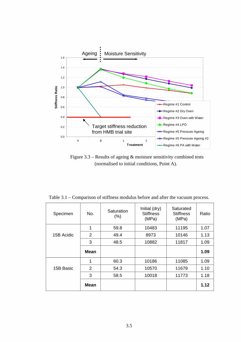
3.5

Figure 3.3 – Results of ageing & moisture sensitivity combined tests (normalised to initial conditions, Point A).

Table 3.1 – Comparison of stiffness modulus before and after the vacuum process.

Specimen No. Saturation (%)

Initial (dry) Stiffness

(MPa)

Saturated Stiffness

(MPa) Ratio

1 59.8 10483 11195 1.07 15B Acidic 2 49.4 8973 10146 1.13

3 48.5 10882 11817 1.09

Mean 1.09

1 60.3 10186 11085 1.09 15B Basic 2 54.3 10570 11679 1.10

3 58.5 10018 11773 1.18

Mean 1.12

0.0

0.2

0.4

0.6

0.8

1.0

1.2

1.4

1.6

A B 1 2 3 4Treatment

Stiff

ness

Rat

io

Regime #1 Control

Regime #2 Dry Oven

Regime #3 Oven with Water

Regime #4 LPO

Regime #5 Pressure Ageing

Regime #5 Pressure Ageing #2

Regime #6 PA with Water

Moisture Sensitivity Ageing

Target stiffness reduction from HMB trial site

3.6

It can be seen from Figures 3.2 and 3.3 that the oven aged specimens with and

without moisture (Regimes #2 and #3) showed very similar ageing sensitivity with

up to a 37% increase in stiffness modulus after ageing. Regime #2 then showed a

28% reduction in stiffness modulus whilst regime #3 showed a 24% reduction in

stiffness modulus due to moisture damage. It is clear that the additional humidity of

Regime #3 did not create a more severe ageing/moisture damage environment

(compared to Regime #2).

It can also be seen from Figures 3.2 and 3.3 that Regime #4 (LPO) showed a very

similar ageing sensitivity (36% increase in stiffness modulus) compared to the oven

ageing (Regimes #2 and #3). It could be assumed that, since the material has a high

air void content (≈ 8%), the hot air could freely flow inside the specimen without

being forced.

Figures 3.2 and 3.3 show that the HiPAT aged specimens (Regime #5, 2 repetitions)

showed the least ageing and the most moisture sensitivity. The stiffness modulus

increased by only 5% after ageing and then decreased by 40% due to moisture

damage.

As shown in Figure 3.3, the saturated HiPAT aged specimens (Regime #6) showed

the most severe behaviour even before undergoing the moisture conditioning

process. After the ageing process, the stiffness modulus dropped to approximately

40% of its initial value (i.e. a 60% reduction).

The HiPAT aged regimes without/with moisture (Regimes #5 and #6) appear to

make specimens more susceptible to the following moisture conditioning (Regime

#5) or incorporated saturated water (Regime #6). It is assumed that the high pressure

inside the vessel has induced a certain type of internal damage (e.g. micro-cracking),

which has enabled water to infiltrate more easily to the specimen. A more detailed

investigation of the high pressure effect on compacted specimens is presented in

Chapter 7.

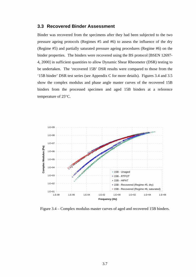
3.7

3.3 Recovered Binder Assessment

Binder was recovered from the specimens after they had been subjected to the two

pressure ageing protocols (Regimes #5 and #6) to assess the influence of the dry

(Regime #5) and partially saturated pressure ageing procedures (Regime #6) on the

binder properties. The binders were recovered using the BS protocol [BSEN 12697-

4, 2000] in sufficient quantities to allow Dynamic Shear Rheometer (DSR) testing to

be undertaken. The ‘recovered 15B’ DSR results were compared to those from the

‘15B binder’ DSR test series (see Appendix C for more details). Figures 3.4 and 3.5

show the complex modulus and phase angle master curves of the recovered 15B

binders from the processed specimen and aged 15B binders at a reference

temperature of 25°C.

1.E+01

1.E+02

1.E+03

1.E+04

1.E+05

1.E+06

1.E+07

1.E+08

1.E+09

1.E-08 1.E-06 1.E-04 1.E-02 1.E+00 1.E+02 1.E+04 1.E+06

Frequency (Hz)

Com

plex

Mod

ulus

(Pa)

15B - Unaged

15B - RTFOT

15B - HiPAT

15B - Recovered (Regime #5, dry)

15B - Recovered (Regime #6, saturated)

Figure 3.4 – Complex modulus master curves of aged and recovered 15B binders.

3.8

0

10

20

30

40

50

60

70

80

90

1.E-09 1.E-07 1.E-05 1.E-03 1.E-01 1.E+01 1.E+03 1.E+05 1.E+07

Frequency (Hz)

Phas

e A

ngle

(deg

rees

)

15B - Unaged15B - RTFO15B - HiPAT15B - Recovered (Regime #5, dry)15B - Recovered (Regime #6, saturated)

Figure 3.5 – Phase angle master curves of aged and recovered 15B binder.

These figures clearly show that the binders recovered from specimens tested using

Regimes #5 and #6 have reasonably similar rheological characteristics to those of the

HiPAT aged binder. It can therefore be concluded that the loss of mixture stiffness

modulus observed in Regime #6 is due to moisture damage rather than any alteration

in the rheological characteristics of the binders. Also, regardless of the presence of

water in the pressure vessel, the binder in the mixture is likely to be aged according

to the given HiPAT ageing condition. Further investigation and discussions of the

recovered binder assessment are presented in Chapter 9 (see Section 9.4.2).

3.4 Summary and Conclusions

Among the various regimes tried in this chapter, to find a suitable durability test

method which fulfils the given objectives of this study, the HiPAT ageing using

saturated specimens (Regime #6) showed the most distinctive and interesting

behaviour. Firstly it was the only process which was severe enough to produce the

target stiffness reduction (60%) within reasonably shorter period of time (65 hours).

Secondly it was the only process which had ageing and moisture sensitivity schemes

in ‘one process’.

3.9

The investigation (Section 3.3) on the recovered binder extracted from the specimens

which had been through the Regimes #5 and #6 clearly demonstrated a comparable

level of binder ageing to the standard HiPAT aged binder. Any loss of stiffness

modulus or strength for the moisture aged asphalt mixtures can therefore be

attributed to a loss of the cohesive and/or adhesive properties of the mixture rather

than any unexpected “softening” of the binder.

Knowing that the binder in the mixture will be ‘long-term’ aged according to the

given HiPAT ageing conditions (air temperature of 85oC and pressure of 2.1 MPa),

while the mixture is ‘moisture damaged’ by saturated water in the pressure vessel

(water temperature of 85oC), Regime #6 approach showed a strong possibility to be a

suitable durability test method which fulfils the given objectives of this study (see

Section 1.2). Thus the following chapters will describe the investigation and

development of the PAV with water ageing protocols (referred to as the Saturated

Ageing Tensile Stiffness, SATS, test).

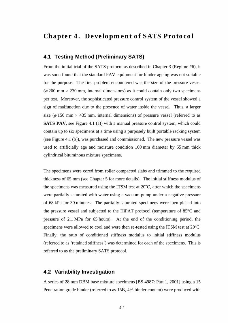
4.1

Chapter 4. Development of SATS Protocol

4.1 Testing Method (Preliminary SATS)

From the initial trial of the SATS protocol as described in Chapter 3 (Regime #6), it

was soon found that the standard PAV equipment for binder ageing was not suitable

for the purpose. The first problem encountered was the size of the pressure vessel

(φ 200 mm × 230 mm, internal dimensions) as it could contain only two specimens

per test. Moreover, the sophisticated pressure control system of the vessel showed a

sign of malfunction due to the presence of water inside the vessel. Thus, a larger

size (φ 150 mm × 435 mm, internal dimensions) of pressure vessel (referred to as

SATS PAV, see Figure 4.1 (a)) with a manual pressure control system, which could

contain up to six specimens at a time using a purposely built portable racking system

(see Figure 4.1 (b)), was purchased and commissioned. The new pressure vessel was

used to artificially age and moisture condition 100 mm diameter by 65 mm thick

cylindrical bituminous mixture specimens.

The specimens were cored from roller compacted slabs and trimmed to the required

thickness of 65 mm (see Chapter 5 for more details). The initial stiffness modulus of

the specimens was measured using the ITSM test at 20oC, after which the specimens

were partially saturated with water using a vacuum pump under a negative pressure

of 68 kPa for 30 minutes. The partially saturated specimens were then placed into

the pressure vessel and subjected to the HiPAT protocol (temperature of 85°C and

pressure of 2.1 MPa for 65 hours). At the end of the conditioning period, the

specimens were allowed to cool and were then re-tested using the ITSM test at 20oC.

Finally, the ratio of conditioned stiffness modulus to initial stiffness modulus

(referred to as ‘retained stiffness’) was determined for each of the specimens. This is

referred to as the preliminary SATS protocol.

4.2 Variability Investigation

A series of 28 mm DBM base mixture specimens [BS 4987: Part 1, 2001] using a 15

Penetration grade binder (referred to as 15B, 4% binder content) were produced with

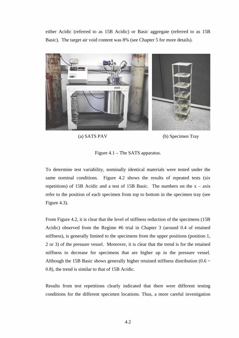
4.2

either Acidic (referred to as 15B Acidic) or Basic aggregate (referred to as 15B

Basic). The target air void content was 8% (see Chapter 5 for more details).

(a) SATS PAV (b) Specimen Tray

Figure 4.1 – The SATS apparatus.

To determine test variability, nominally identical materials were tested under the

same nominal conditions. Figure 4.2 shows the results of repeated tests (six

repetitions) of 15B Acidic and a test of 15B Basic. The numbers on the x – axis

refer to the position of each specimen from top to bottom in the specimen tray (see

Figure 4.3).

From Figure 4.2, it is clear that the level of stiffness reduction of the specimens (15B

Acidic) observed from the Regime #6 trial in Chapter 3 (around 0.4 of retained

stiffness), is generally limited to the specimens from the upper positions (position 1,

2 or 3) of the pressure vessel. Moreover, it is clear that the trend is for the retained

stiffness to decrease for specimens that are higher up in the pressure vessel.

Although the 15B Basic shows generally higher retained stiffness distribution (0.6 ~

0.8), the trend is similar to that of 15B Acidic.

Results from test repetitions clearly indicated that there were different testing

conditions for the different specimen locations. Thus, a more careful investigation

4.3

was performed to investigate the test conditions within the vessel and the key factors

controlling the moisture damage.

Figure 4.2 – Results from repeated preliminary SATS test on 15B Acidic

and Basic specimens.

Figure 4.3 – Schematic diagram of preliminary SATS setup.

Specimen Tray

1st

2nd

3rd

4th

6th

Pressure Vessel

5th

0.0

0.1

0.2

0.3

0.4

0.5

0.6

0.7

0.8

0.9

1.0

1 2 3 4 5 6

Ret

aine

d St

iffne

ss15B Basic

15B Acidic

Top Bottom

4.4

4.3 Detailed Investigation of the SATS Setup

4.3.1 Temperature

Figure 4.4 shows a schematic diagram illustrating the SATS PAV heating elements.

A set of dummy specimens with thermocouples inserted in them was placed in the

vessel and the target temperature (85oC) was controlled. Atmospheric pressure was

used for this investigation (no additionally applied pressure).

It can be seen from Figure 4.4 that the temperature difference between specimens

located at the top and bottom of the vessel was approximately 13oC. The reason was

thought to be due to the combination of heat loss though the vessel cover and the fact

that the main heating element is located at the base of the vessel. Also it should be

noted that there is no internal forced air circulation (the source apparatus is actually

intended to house a liquid medium).

To investigate the effect of this temperature variation on ageing of the bituminous

material, six identical ‘dry’ specimens (15B Acidic) were tested in the vessel using

the HiPAT protocols (referred to as ‘Dry HiPAT’). The results are shown in

Figure 4.5. It can be seen from this figure that the retained stiffness modulus vary

from approximately 1.00 (Positions 2 and 3) to 1.15 (location 5) which are very

similar values observed from the Regime #5 (after HiPAT ageing) in Chapter 3.

The standard PAV used in preliminary trials in Chapter 3 has about a half height of

the SATS PAV and has a proper insulation around the vessel (including the top

cover). Therefore it is expected to have a much smaller temperature variation (only

two specimens per test). As the specimen ageing under 13oC difference showed very

similar values to those from the standard PAV, without a distinctive trend to the

position of the specimen (as shown in Figure 4.2), it is presumed that the

temperature variation in the SATS PAV has a very minor effect on the results

observed in Section 4.2.

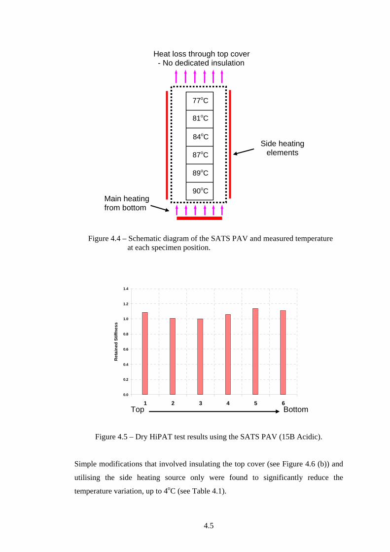
4.5

Figure 4.4 – Schematic diagram of the SATS PAV and measured temperature at each specimen position.

Figure 4.5 – Dry HiPAT test results using the SATS PAV (15B Acidic).

Simple modifications that involved insulating the top cover (see Figure 4.6 (b)) and

utilising the side heating source only were found to significantly reduce the

temperature variation, up to 4oC (see Table 4.1).

0.0

0.2

0.4

0.6

0.8

1.0

1.2

1.4

1 2 3 4 5 6

Ret

aine

d St

iffne

ss

Top Bottom

Side heating elements

Main heating from bottom

Heat loss through top cover - No dedicated insulation

77oC

81oC

84oC

87oC

89oC

90oC

4.6

Table 4.1 – Modification of the SATS PAV to minimise temperature variation.

Target temperature of 85oC Max Temp. (oC)

Min Temp. (oC)

Variation (oC)

Normal setup 90 77 13

Insulation on top cover 86 80 6

Side heating source only (+ insulation on top cover) 86 82 4

(a) Normal setup (b) Top cover insulation

Figure 4.6 – Insulation on top cover of SATS PAV

4.3.2 Saturation

Once the specimens are vacuum saturated and placed in the vessel, as described in

Section 4.1, it is likely that a certain portion of the saturated water will evaporate or

drain from each specimen and circulate inside the vessel. Consequently, due to the

temperature difference between the inside of the vessel (≈ 85oC) and the outside

atmosphere (≈ 20oC), and also knowing that the side wall of the vessel is surround by

heating elements (see Figure 4.4), evaporated moisture will be ‘condensed’ mostly

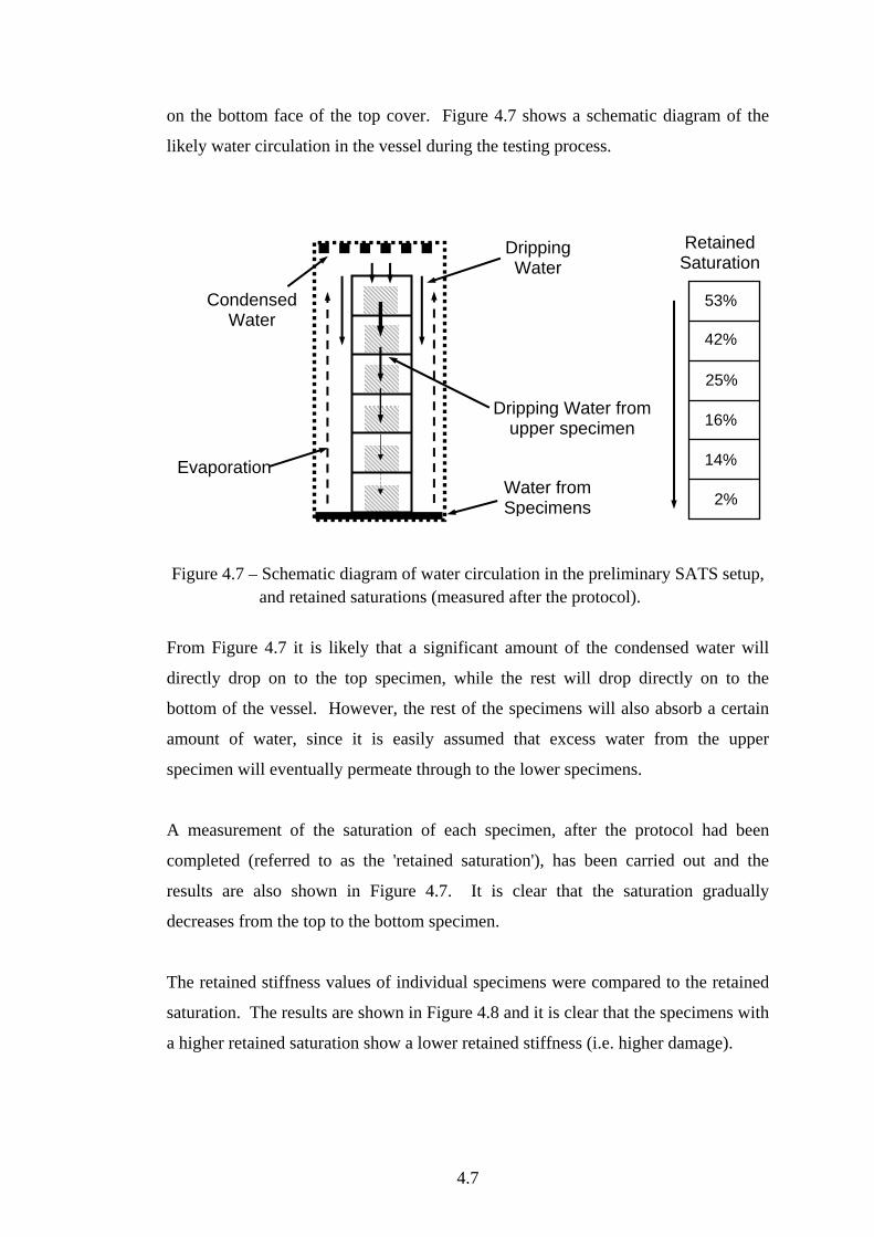
4.7

on the bottom face of the top cover. Figure 4.7 shows a schematic diagram of the

likely water circulation in the vessel during the testing process.

Figure 4.7 – Schematic diagram of water circulation in the preliminary SATS setup, and retained saturations (measured after the protocol).

From Figure 4.7 it is likely that a significant amount of the condensed water will

directly drop on to the top specimen, while the rest will drop directly on to the

bottom of the vessel. However, the rest of the specimens will also absorb a certain

amount of water, since it is easily assumed that excess water from the upper

specimen will eventually permeate through to the lower specimens.

A measurement of the saturation of each specimen, after the protocol had been

completed (referred to as the 'retained saturation'), has been carried out and the

results are also shown in Figure 4.7. It is clear that the saturation gradually

decreases from the top to the bottom specimen.

The retained stiffness values of individual specimens were compared to the retained

saturation. The results are shown in Figure 4.8 and it is clear that the specimens with

a higher retained saturation show a lower retained stiffness (i.e. higher damage).

Water from Specimens

Evaporation

53%

42%

25%

16%

14%

2%

Condensed Water

Dripping Water

Dripping Water from upper specimen

Retained Saturation

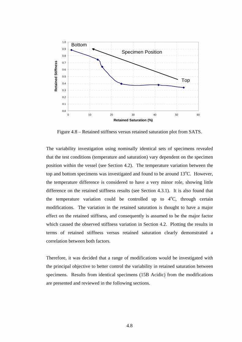
4.8

Figure 4.8 – Retained stiffness versus retained saturation plot from SATS.

The variability investigation using nominally identical sets of specimens revealed

that the test conditions (temperature and saturation) vary dependent on the specimen

position within the vessel (see Section 4.2). The temperature variation between the

top and bottom specimens was investigated and found to be around 13oC. However,

the temperature difference is considered to have a very minor role, showing little

difference on the retained stiffness results (see Section 4.3.1). It is also found that

the temperature variation could be controlled up to 4oC, through certain

modifications. The variation in the retained saturation is thought to have a major

effect on the retained stiffness, and consequently is assumed to be the major factor

which caused the observed stiffness variation in Section 4.2. Plotting the results in

terms of retained stiffness versus retained saturation clearly demonstrated a

correlation between both factors.

Therefore, it was decided that a range of modifications would be investigated with

the principal objective to better control the variability in retained saturation between

specimens. Results from identical specimens (15B Acidic) from the modifications

are presented and reviewed in the following sections.

0.0

0.1

0.2

0.3

0.4

0.5

0.6

0.7

0.8

0.9

1.0

0 10 20 30 40 50 60

Retained Saturation (%)

Ret

aine

d St

iffne

ss

Top

Bottom Specimen Position

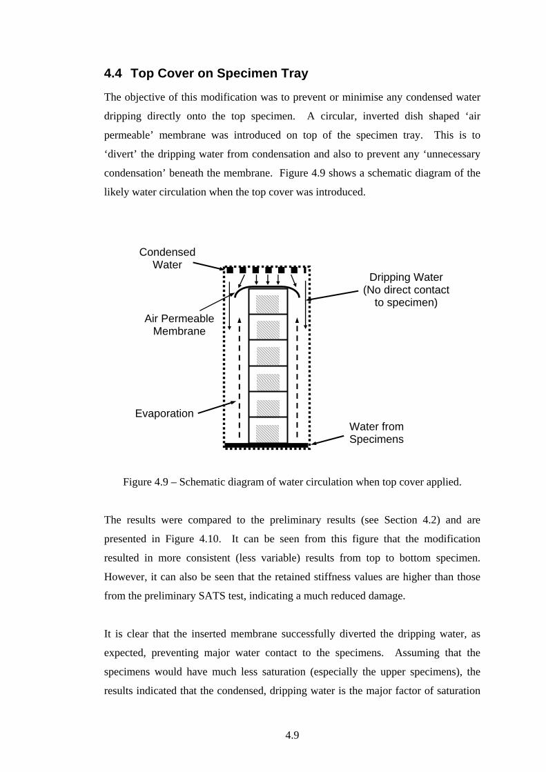
4.9

4.4 Top Cover on Specimen Tray

The objective of this modification was to prevent or minimise any condensed water

dripping directly onto the top specimen. A circular, inverted dish shaped ‘air

permeable’ membrane was introduced on top of the specimen tray. This is to

‘divert’ the dripping water from condensation and also to prevent any ‘unnecessary

condensation’ beneath the membrane. Figure 4.9 shows a schematic diagram of the

likely water circulation when the top cover was introduced.

Figure 4.9 – Schematic diagram of water circulation when top cover applied.

The results were compared to the preliminary results (see Section 4.2) and are

presented in Figure 4.10. It can be seen from this figure that the modification

resulted in more consistent (less variable) results from top to bottom specimen.

However, it can also be seen that the retained stiffness values are higher than those

from the preliminary SATS test, indicating a much reduced damage.

It is clear that the inserted membrane successfully diverted the dripping water, as

expected, preventing major water contact to the specimens. Assuming that the

specimens would have much less saturation (especially the upper specimens), the

results indicated that the condensed, dripping water is the major factor of saturation

Water from Specimens

Evaporation

Condensed Water

Dripping Water (No direct contact

to specimen) Air Permeable

Membrane

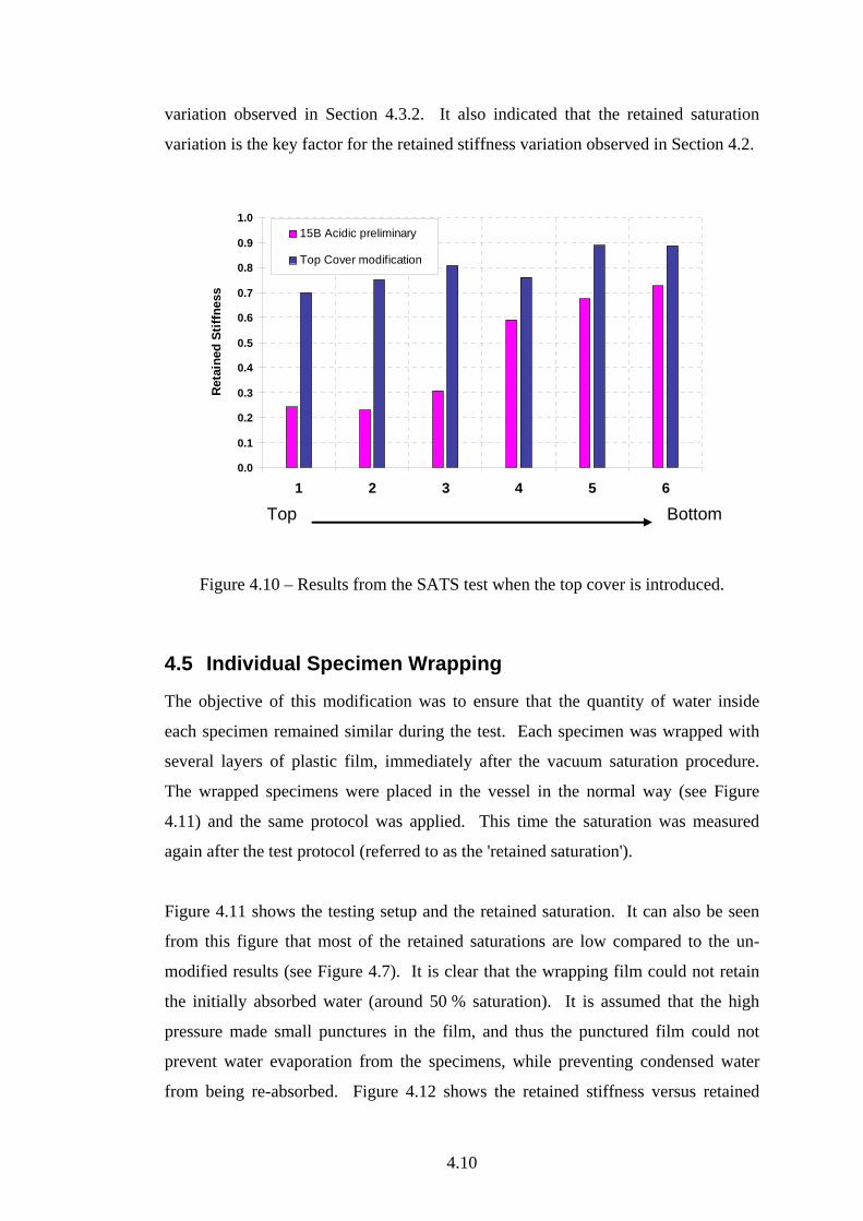
4.10

variation observed in Section 4.3.2. It also indicated that the retained saturation

variation is the key factor for the retained stiffness variation observed in Section 4.2.

Figure 4.10 – Results from the SATS test when the top cover is introduced.

4.5 Individual Specimen Wrapping

The objective of this modification was to ensure that the quantity of water inside

each specimen remained similar during the test. Each specimen was wrapped with

several layers of plastic film, immediately after the vacuum saturation procedure.

The wrapped specimens were placed in the vessel in the normal way (see Figure

4.11) and the same protocol was applied. This time the saturation was measured

again after the test protocol (referred to as the 'retained saturation').

Figure 4.11 shows the testing setup and the retained saturation. It can also be seen

from this figure that most of the retained saturations are low compared to the un-

modified results (see Figure 4.7). It is clear that the wrapping film could not retain

the initially absorbed water (around 50 % saturation). It is assumed that the high

pressure made small punctures in the film, and thus the punctured film could not

prevent water evaporation from the specimens, while preventing condensed water

from being re-absorbed. Figure 4.12 shows the retained stiffness versus retained

0.0

0.1

0.2

0.3

0.4

0.5

0.6

0.7

0.8

0.9

1.0

1 2 3 4 5 6

Ret

aine

d St

iffne

ss15B Acidic preliminary

Top Cover modification

Top Bottom

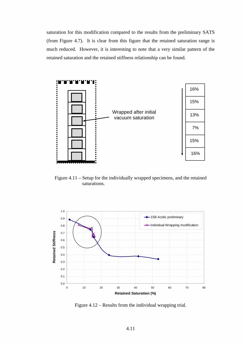
4.11

saturation for this modification compared to the results from the preliminary SATS

(from Figure 4.7). It is clear from this figure that the retained saturation range is

much reduced. However, it is interesting to note that a very similar pattern of the

retained saturation and the retained stiffness relationship can be found.

Figure 4.11 – Setup for the individually wrapped specimens, and the retained saturations.

Figure 4.12 – Results from the individual wrapping trial.

16%

15%

13%

7%

15%

16%

Wrapped after initial vacuum saturation

0.0

0.1

0.2

0.3

0.4

0.5

0.6

0.7

0.8

0.9

1.0

0 10 20 30 40 50 60 70 80

Retained Saturation (%)

Ret

aine

d St

iffne

ss

15B Acidic preliminary

Individual Wrapping modification

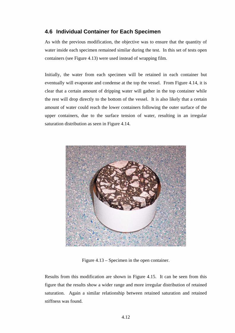
4.12

4.6 Individual Container for Each Specimen

As with the previous modification, the objective was to ensure that the quantity of

water inside each specimen remained similar during the test. In this set of tests open

containers (see Figure 4.13) were used instead of wrapping film.

Initially, the water from each specimen will be retained in each container but

eventually will evaporate and condense at the top the vessel. From Figure 4.14, it is

clear that a certain amount of dripping water will gather in the top container while

the rest will drop directly to the bottom of the vessel. It is also likely that a certain

amount of water could reach the lower containers following the outer surface of the

upper containers, due to the surface tension of water, resulting in an irregular

saturation distribution as seen in Figure 4.14.

Figure 4.13 – Specimen in the open container.

Results from this modification are shown in Figure 4.15. It can be seen from this

figure that the results show a wider range and more irregular distribution of retained

saturation. Again a similar relationship between retained saturation and retained

stiffness was found.

4.13

Figure 4.14 – Schematic diagram of water circulation with the open containers, and retained saturation.

Figure 4.15 – Results from the individual container trial.

4.7 Middle Collar in Tray

The objective of this modification was to increase the saturation levels of the lower

specimens (positions 4, 5 and 6). A water collecting collar, comprising an air

permeable membrane as described in Section 4.4, was inserted in the middle of the

specimen tray as shown in Figure 4.16. It was anticipated that the collar would

26%

19%

23%

13%

7%

5%

Open Container

Evaporation

Dripping Water

0.0

0.1

0.2

0.3

0.4

0.5

0.6

0.7

0.8

0.9

1.0

0 10 20 30 40 50 60

Retained Saturation (%)

Ret

aine

d St

iffne

ss

15B Acidic preliminary

Individual Wrapping

Individual Container

4.14

collect the dripping water of around the specimen, otherwise directly to the bottom

the vessel, to supply it to the specimens in the lower half of the vessel.

Figure 4.16 – Schematic diagram of water circulation with the middle collar introduced.

It can be seen from Figure 4.16 that the distribution of retained saturation is quite

irregular. The reason for this is not clear but is likely to be due to the

design/manufacture of the collar. The retained stiffnesses are shown in Figure 4.17.

It can be seen from this figure that, although there is an irregular distribution of

retained saturation, the correlation between the retained stiffnesses and retained

saturation is similar to those observed before.

4.8 Semi Immersion SATS

To investigate damage caused by even higher retained saturation levels, additional

water was added to the vessel to immerse the bottom two specimens (see Figure

4.18).

Five specimens were used to simplify the water level control (otherwise one

specimen would be partially immersed). The results indicated that, overall, the

specimens showed higher retained saturations, with the immersed specimens

32%

10%

31%

7%

4%

22%

Collar (Air permeable

membrane)

Evaporation

Dripping Water

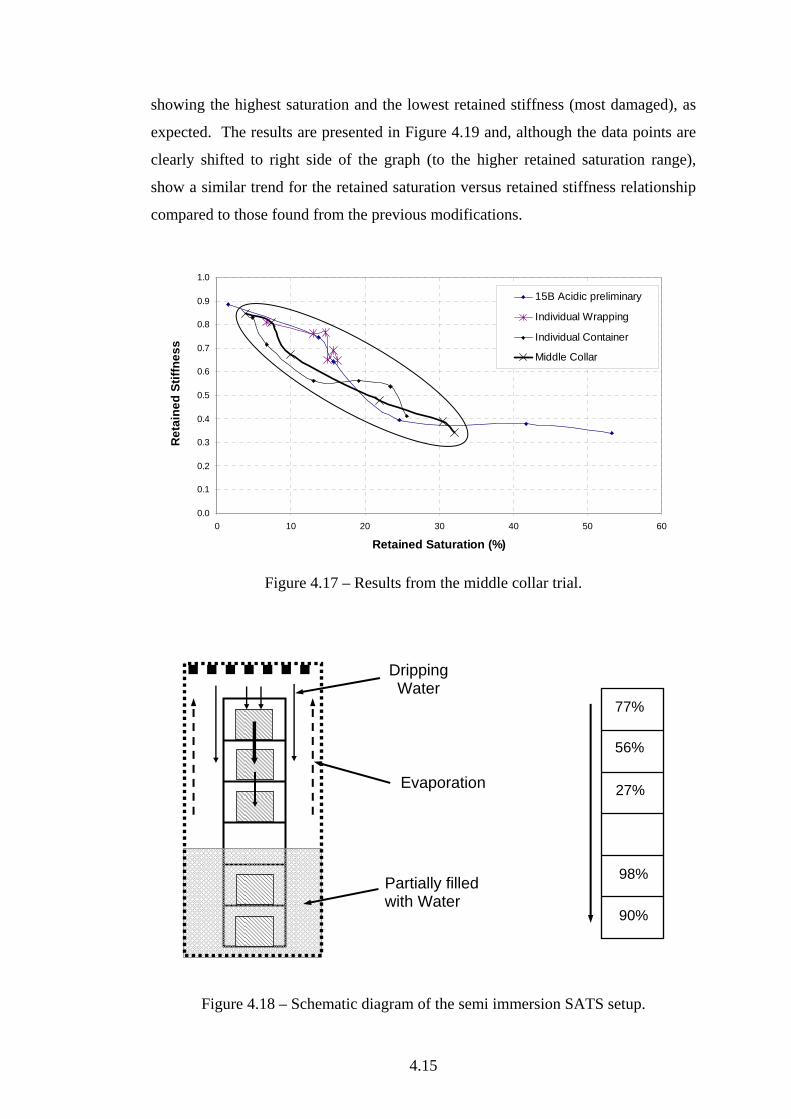
4.15

showing the highest saturation and the lowest retained stiffness (most damaged), as

expected. The results are presented in Figure 4.19 and, although the data points are

clearly shifted to right side of the graph (to the higher retained saturation range),

show a similar trend for the retained saturation versus retained stiffness relationship

compared to those found from the previous modifications.

Figure 4.17 – Results from the middle collar trial.

Figure 4.18 – Schematic diagram of the semi immersion SATS setup.

77%

56%

27%

98%

90%

Evaporation

Partially filled with Water

Dripping Water

0.0

0.1

0.2

0.3

0.4

0.5

0.6

0.7

0.8

0.9

1.0

0 10 20 30 40 50 60

Retained Saturation (%)

Ret

aine

d St

iffne

ss

15B Acidic preliminary

Individual Wrapping

Individual Container

Middle Collar

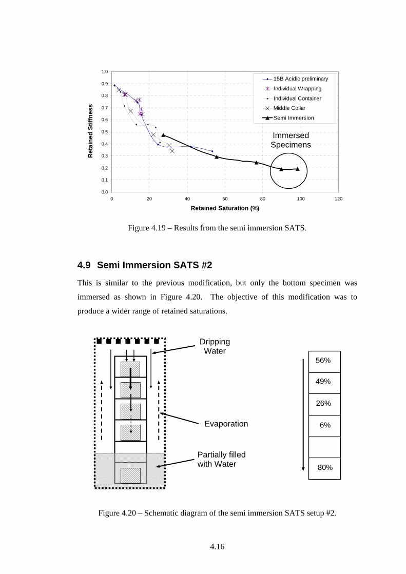
4.16

Figure 4.19 – Results from the semi immersion SATS.

4.9 Semi Immersion SATS #2

This is similar to the previous modification, but only the bottom specimen was

immersed as shown in Figure 4.20. The objective of this modification was to

produce a wider range of retained saturations.

Figure 4.20 – Schematic diagram of the semi immersion SATS setup #2.

0.0

0.1

0.2

0.3

0.4

0.5

0.6

0.7

0.8

0.9

1.0

0 20 40 60 80 100 120

Retained Saturation (%)

Ret

aine

d St

iffne

ss

15B Acidic preliminary

Individual Wrapping

Individual Container

Middle Collar

Semi Immersion

Immersed Specimens

56%

49%

26%

6%

80%

Evaporation

Partially filled with Water

Dripping Water

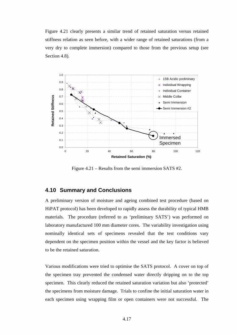
4.17

Figure 4.21 clearly presents a similar trend of retained saturation versus retained

stiffness relation as seen before, with a wider range of retained saturations (from a

very dry to complete immersion) compared to those from the previous setup (see

Section 4.8).

Figure 4.21 – Results from the semi immersion SATS #2.

4.10 Summary and Conclusions

A preliminary version of moisture and ageing combined test procedure (based on

HiPAT protocol) has been developed to rapidly assess the durability of typical HMB

materials. The procedure (referred to as ‘preliminary SATS’) was performed on

laboratory manufactured 100 mm diameter cores. The variability investigation using

nominally identical sets of specimens revealed that the test conditions vary

dependent on the specimen position within the vessel and the key factor is believed

to be the retained saturation.

Various modifications were tried to optimise the SATS protocol. A cover on top of

the specimen tray prevented the condensed water directly dripping on to the top

specimen. This clearly reduced the retained saturation variation but also ‘protected’

the specimens from moisture damage. Trials to confine the initial saturation water in

each specimen using wrapping film or open containers were not successful. The

0.0

0.1

0.2

0.3

0.4

0.5

0.6

0.7

0.8

0.9

1.0

0 20 40 60 80 100 120

Retained Saturation (%)

Ret

aine

d St

iffne

ss

15B Acidic preliminary

Individual Wrapping

Individual Container

Middle Collar

Semi Immersion

Semi Immersion #2

Immersed Specimen

4.18

wrapping film could not hold the high pressure, and the retained water in the

individual containers eventually evaporated. A trial to insert a water collecting

collar in the middle of the specimen tray was also not successful, and it appeared that

a much more complicated design and accurate manufacture of the collar shape would

be required to achieve success.

An alternative approach was tried involving adding more water to the vessel. The

bottom specimen was completely immersed and no other modification applied. The

results showed a more distinctive retained saturation variation from the completely

immersed specimen (nearly 100% retained saturation) to a virtually dry specimen

immediately above the water.

It is interesting to note that the results from all the various modifications generally

fitted in a single retained saturation/retained stiffness correlation curve. The results

therefore suggested that the correlation of retained saturation and retained stiffness,

plotted in a single curve, could be an ideal parameter to indicate the ageing and

moisture related durability of a bituminous mixture.

It is concluded that the retained saturation is the key factor to control the damage

created by the SATS protocol. It is also found that a certain level of retained

saturation variation depending on the specimen location is inevitable and therefore

need to be accepted as a test parameter.

Considering the practicability and repeatability of the protocol, the partially

immersed SATS trial (see Section 4.9) appeared to be the most suitable approach, as

it produces from a very dry specimen to a completely immersed specimen with

gradually saturated specimens between them. Therefore, the partially immersed

SATS as described in Section 4.9 was chosen as the main test protocol for this study,

and referred to as ‘standard SATS’ (or SATS) protocol for the rest part of this thesis.

5.1

Chapter 5. SATS Durability Test

5.1 Materials

The specification for 28 mm DBM base material [BS 4987: Part 1, 2001] was used

to produce a series of mixtures to replicate the material used in the HMB trial site

described in Chapter 1, and to investigate the influence of various mixture

components on the test results, and its variability. The following sections describe

the details of materials, testing protocols and analysis of the results.

5.1.1 Binders

Three 15 Penetration grade binders (referred to as 15B, 15D and 15E) and a

50 Penetration grade binder (50C) were used (4% Binder Content). The details of

the various characteristics of these binders are presented in Appendix C.

5.1.2 Aggregates

A typical acidic aggregate (referred to as ‘Acidic’) and a typical alkaline aggregate

(referred to as ‘Basic’) were used. The Acidic aggregate source was that the same as

that used in the HMB trial site described in Chapter 1. Figure 5.1 shows the

gradations of both aggregates compared against the 28mm DBM base specification

[BS 4987: Part 1, 2001].

5.2 Sample Manufacture

5.2.1 Maximum Density

Rice density test was performed to determine the maximum densities of the Acidic

and Basic mixtures [BSEN 12697: Part 5, 2002]. Values of 2.493 (Mg/m3) and

2.479 (Mg/m3) were obtained for the Acidic and Basic mixtures respectively.

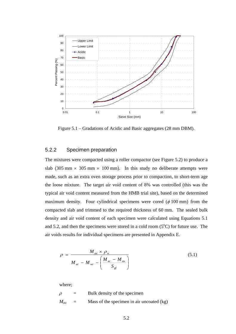
5.2

0

10

20

30

40

50

60

70

80

90

100

0.01 0.1 1 10 100

Sieve Size (mm)

Per

cent

Pas

sing

(%)

Upper Limit

Lower Limit

Acidic

Basic

Figure 5.1 – Gradations of Acidic and Basic aggregates (28 mm DBM).

5.2.2 Specimen preparation

The mixtures were compacted using a roller compactor (see Figure 5.2) to produce a

slab (305 mm × 305 mm × 100 mm). In this study no deliberate attempts were

made, such as an extra oven storage process prior to compaction, to short-term age

the loose mixture. The target air void content of 8% was controlled (this was the

typical air void content measured from the HMB trial site), based on the determined

maximum density. Four cylindrical specimens were cored (φ 100 mm) from the

compacted slab and trimmed to the required thickness of 60 mm. The sealed bulk

density and air void content of each specimen were calculated using Equations 5.1

and 5.2, and then the specimens were stored in a cold room (5oC) for future use. The

air voids results for individual specimens are presented in Appendix E.

⎟⎟⎠

⎞⎜⎜⎝

⎛ −−−

×=

gf

auacwcac

wau

SMM

MM

M ρρ (5.1)

where;

ρ = Bulk density of the specimen

Mau = Mass of the specimen in air uncoated (kg)

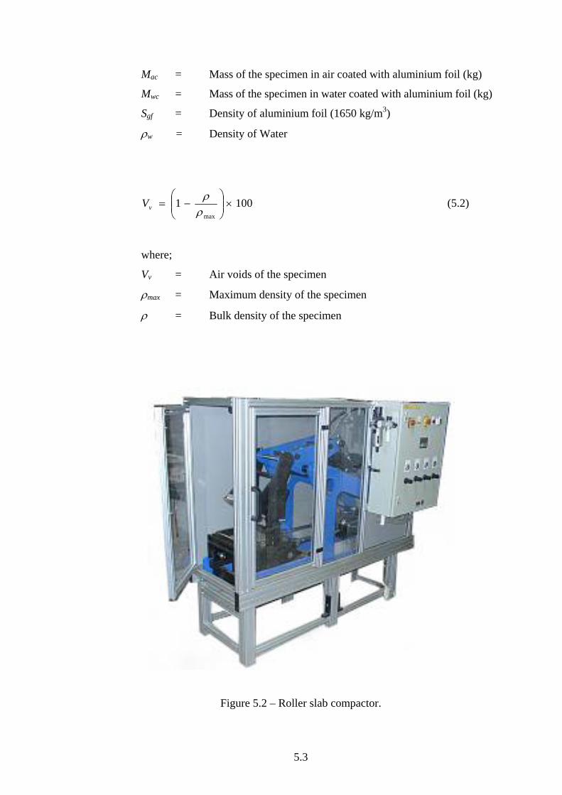
5.3

Mac = Mass of the specimen in air coated with aluminium foil (kg)

Mwc = Mass of the specimen in water coated with aluminium foil (kg)

Sgf = Density of aluminium foil (1650 kg/m3)

ρw = Density of Water

1001max

×⎟⎟⎠

⎞⎜⎜⎝

⎛−=ρρ

vV (5.2)

where;

Vv = Air voids of the specimen

ρmax = Maximum density of the specimen

ρ = Bulk density of the specimen

Figure 5.2 – Roller slab compactor.

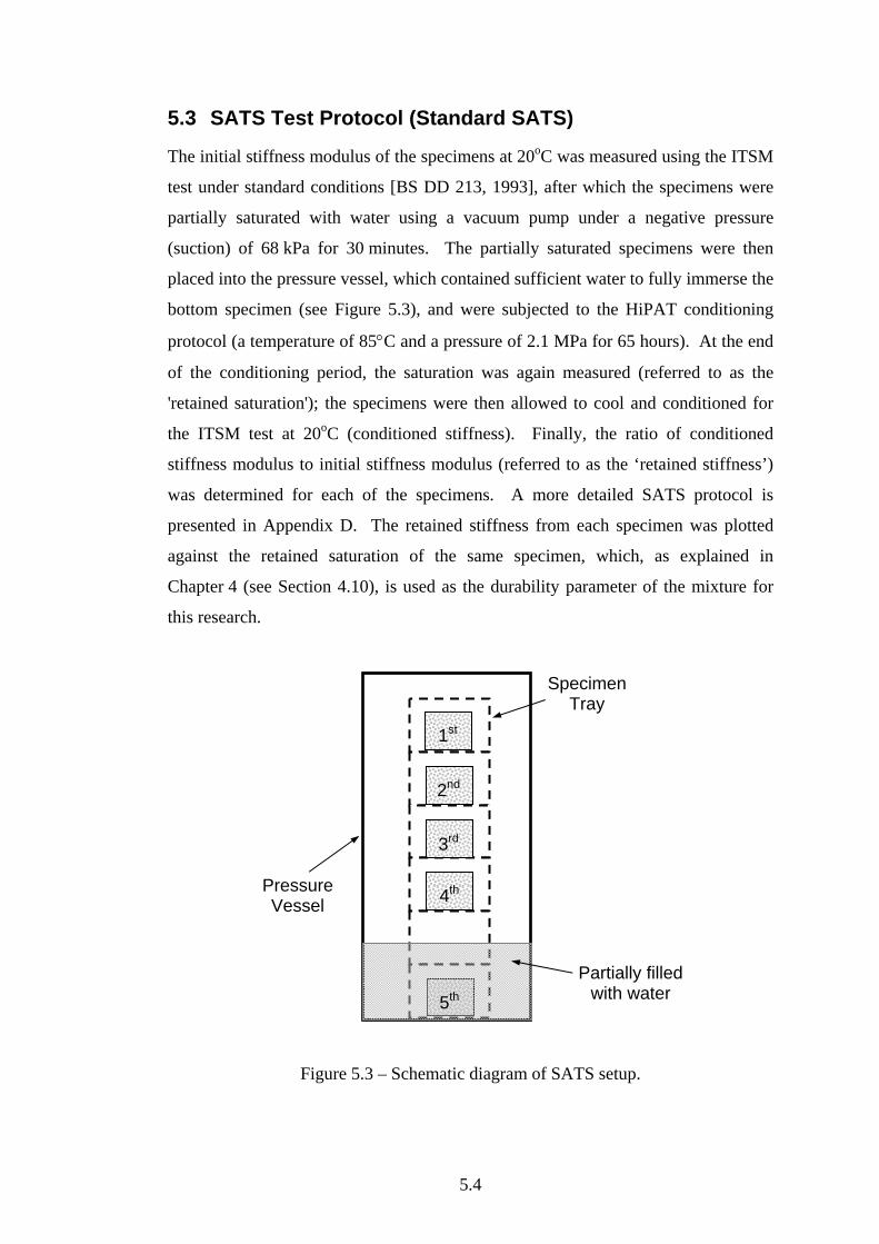
5.4

5.3 SATS Test Protocol (Standard SATS)

The initial stiffness modulus of the specimens at 20oC was measured using the ITSM

test under standard conditions [BS DD 213, 1993], after which the specimens were

partially saturated with water using a vacuum pump under a negative pressure

(suction) of 68 kPa for 30 minutes. The partially saturated specimens were then

placed into the pressure vessel, which contained sufficient water to fully immerse the

bottom specimen (see Figure 5.3), and were subjected to the HiPAT conditioning

protocol (a temperature of 85°C and a pressure of 2.1 MPa for 65 hours). At the end

of the conditioning period, the saturation was again measured (referred to as the

'retained saturation'); the specimens were then allowed to cool and conditioned for

the ITSM test at 20oC (conditioned stiffness). Finally, the ratio of conditioned

stiffness modulus to initial stiffness modulus (referred to as the ‘retained stiffness’)

was determined for each of the specimens. A more detailed SATS protocol is

presented in Appendix D. The retained stiffness from each specimen was plotted

against the retained saturation of the same specimen, which, as explained in

Chapter 4 (see Section 4.10), is used as the durability parameter of the mixture for

this research.

Figure 5.3 – Schematic diagram of SATS setup.

Specimen Tray

Partially filled with water

1st

2nd

3rd

4th

5th

Pressure Vessel

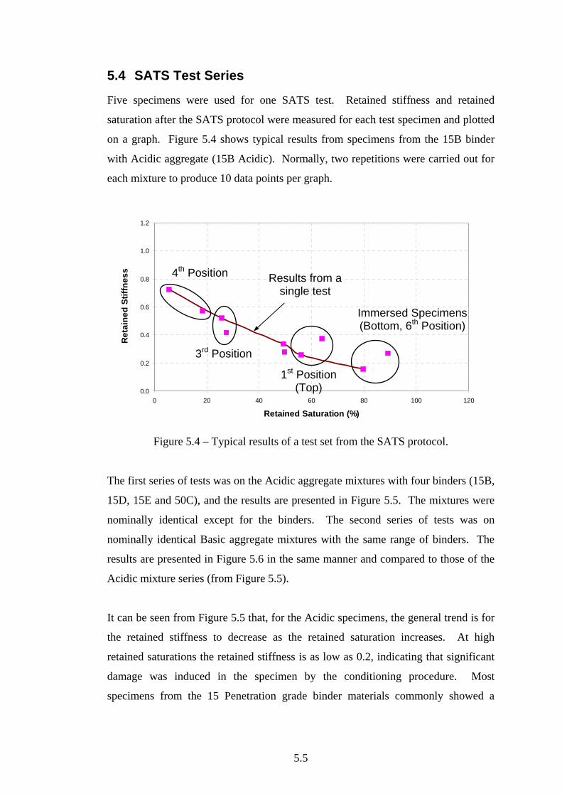
5.5

5.4 SATS Test Series

Five specimens were used for one SATS test. Retained stiffness and retained

saturation after the SATS protocol were measured for each test specimen and plotted

on a graph. Figure 5.4 shows typical results from specimens from the 15B binder

with Acidic aggregate (15B Acidic). Normally, two repetitions were carried out for

each mixture to produce 10 data points per graph.

Figure 5.4 – Typical results of a test set from the SATS protocol.

The first series of tests was on the Acidic aggregate mixtures with four binders (15B,

15D, 15E and 50C), and the results are presented in Figure 5.5. The mixtures were

nominally identical except for the binders. The second series of tests was on

nominally identical Basic aggregate mixtures with the same range of binders. The

results are presented in Figure 5.6 in the same manner and compared to those of the

Acidic mixture series (from Figure 5.5).

It can be seen from Figure 5.5 that, for the Acidic specimens, the general trend is for

the retained stiffness to decrease as the retained saturation increases. At high

retained saturations the retained stiffness is as low as 0.2, indicating that significant

damage was induced in the specimen by the conditioning procedure. Most

specimens from the 15 Penetration grade binder materials commonly showed a

0.0

0.2

0.4

0.6

0.8

1.0

1.2

0 20 40 60 80 100 120

Retained Saturation (%)

Ret

aine

d St

iffne

ss Results from a single test

Immersed Specimens (Bottom, 6th Position)

4th Position

1st Position (Top)

3rd Position

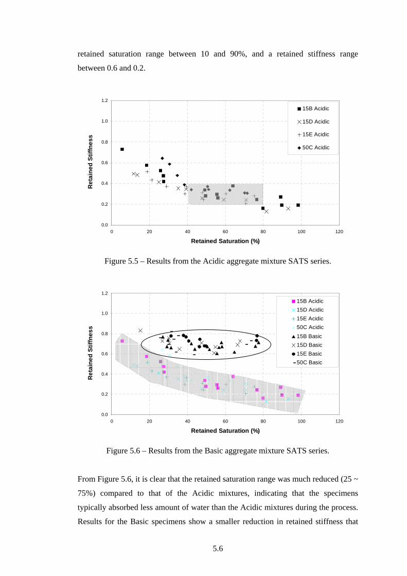
5.6

retained saturation range between 10 and 90%, and a retained stiffness range

between 0.6 and 0.2.

Figure 5.5 – Results from the Acidic aggregate mixture SATS series.

Figure 5.6 – Results from the Basic aggregate mixture SATS series.

From Figure 5.6, it is clear that the retained saturation range was much reduced (25 ~

75%) compared to that of the Acidic mixtures, indicating that the specimens

typically absorbed less amount of water than the Acidic mixtures during the process.

Results for the Basic specimens show a smaller reduction in retained stiffness that

0.0

0.2

0.4

0.6

0.8

1.0

1.2

0 20 40 60 80 100 120

Retained Saturation (%)

Ret

aine

d St

iffne

ss

15B Acidic

15D Acidic

15E Acidic

50C Acidic

0.0

0.2

0.4

0.6

0.8

1.0

1.2

0 20 40 60 80 100 120

Retained Saturation (%)

Ret

aine

d St

iffne

ss

15B Acidic15D Acidic15E Acidic50C Acidic15B Basic15D Basic15E Basic50C Basic

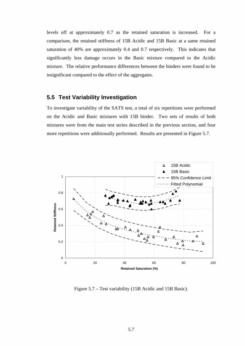
5.7

levels off at approximately 0.7 as the retained saturation is increased. For a

comparison, the retained stiffness of 15B Acidic and 15B Basic at a same retained

saturation of 40% are approximately 0.4 and 0.7 respectively. This indicates that

significantly less damage occurs in the Basic mixture compared to the Acidic

mixture. The relative performance differences between the binders were found to be

insignificant compared to the effect of the aggregates.

5.5 Test Variability Investigation

To investigate variability of the SATS test, a total of six repetitions were performed

on the Acidic and Basic mixtures with 15B binder. Two sets of results of both

mixtures were from the main test series described in the previous section, and four

more repetitions were additionally performed. Results are presented in Figure 5.7.

0

0.2

0.4

0.6

0.8

1

0 20 40 60 80 100

Retained Saturation (%)

Ret

aine

d St

iffne

ss

15B Acidic15B Basic95% Confidence LimitFitted Polynomial

Figure 5.7 – Test variability (15B Acidic and 15B Basic).

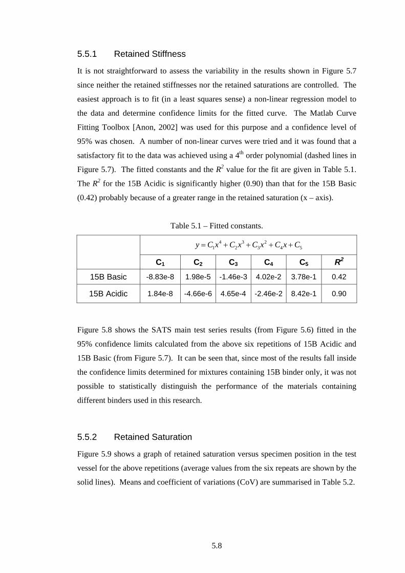
5.8

5.5.1 Retained Stiffness

It is not straightforward to assess the variability in the results shown in Figure 5.7

since neither the retained stiffnesses nor the retained saturations are controlled. The

easiest approach is to fit (in a least squares sense) a non-linear regression model to

the data and determine confidence limits for the fitted curve. The Matlab Curve

Fitting Toolbox [Anon, 2002] was used for this purpose and a confidence level of

95% was chosen. A number of non-linear curves were tried and it was found that a

satisfactory fit to the data was achieved using a 4th order polynomial (dashed lines in

Figure 5.7). The fitted constants and the R2 value for the fit are given in Table 5.1.

The R2 for the 15B Acidic is significantly higher (0.90) than that for the 15B Basic

(0.42) probably because of a greater range in the retained saturation (x – axis).

Table 5.1 – Fitted constants.

542

33

24

1 CxCxCxCxCy ++++=

C1 C2 C3 C4 C5 R2

15B Basic -8.83e-8 1.98e-5 -1.46e-3 4.02e-2 3.78e-1 0.42

15B Acidic 1.84e-8 -4.66e-6 4.65e-4 -2.46e-2 8.42e-1 0.90

Figure 5.8 shows the SATS main test series results (from Figure 5.6) fitted in the

95% confidence limits calculated from the above six repetitions of 15B Acidic and

15B Basic (from Figure 5.7). It can be seen that, since most of the results fall inside

the confidence limits determined for mixtures containing 15B binder only, it was not

possible to statistically distinguish the performance of the materials containing

different binders used in this research.

5.5.2 Retained Saturation

Figure 5.9 shows a graph of retained saturation versus specimen position in the test

vessel for the above repetitions (average values from the six repeats are shown by the

solid lines). Means and coefficient of variations (CoV) are summarised in Table 5.2.

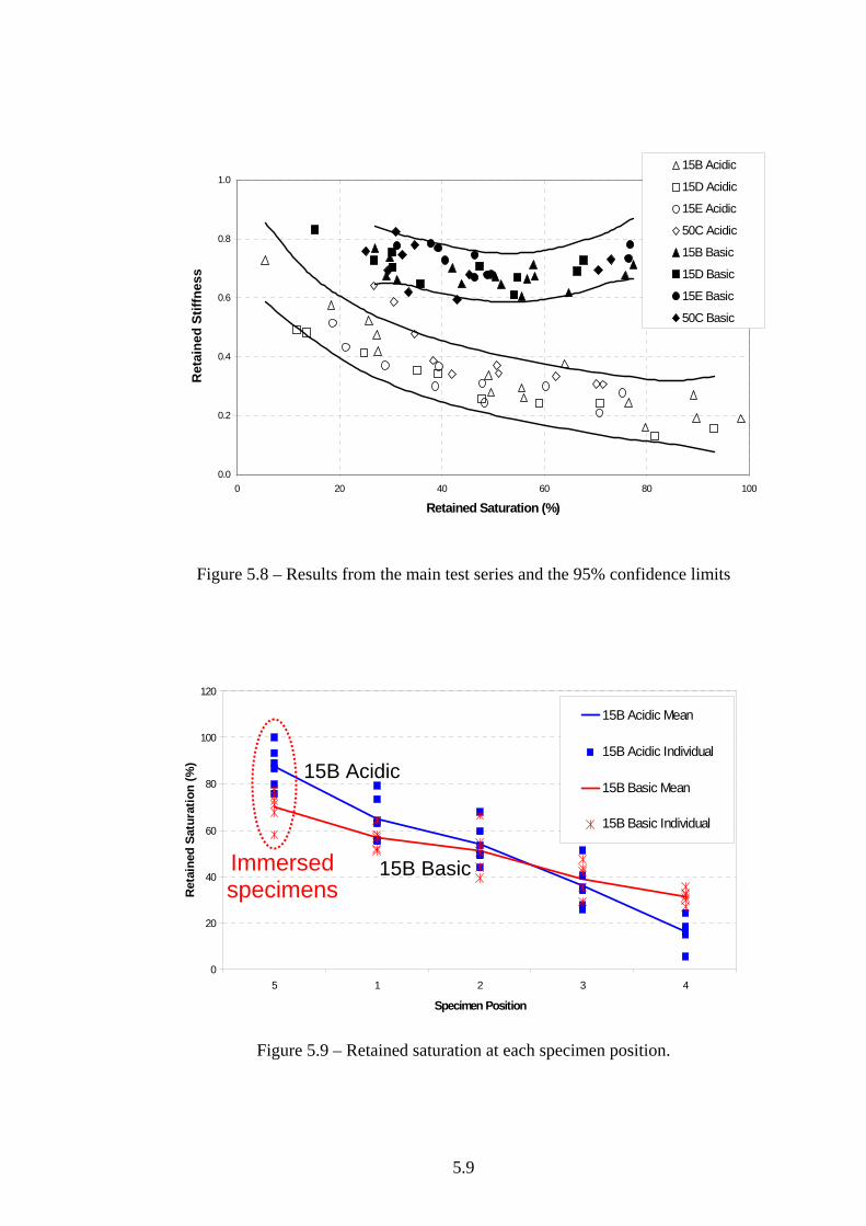
5.9

0.0

0.2

0.4

0.6

0.8

1.0

0 20 40 60 80 100

Retained Saturation (%)

Ret

aine

d St

iffne

ss

15B Acidic

15D Acidic

15E Acidic

50C Acidic

15B Basic

15D Basic

15E Basic

50C Basic

Figure 5.8 – Results from the main test series and the 95% confidence limits

Figure 5.9 – Retained saturation at each specimen position.

0

20

40

60

80

100

120

5 1 2 3 4

Specimen Position

Ret

aine

d Sa

tura

tion

(%)

15B Acidic Mean

15B Acidic Individual

15B Basic Mean

15B Basic Individual

15B Basic

15B Acidic

Immersed specimens

5.10

It can be seen from this figure that, apart from the immersed specimen (5th position

from Figure 5.3), the general trend for both mixtures is for the retained saturation to

decrease for specimens that are located further down inside the pressure vessel. It

can also be seen from this figure that the retained saturation for the specimens above

the water level ranges from 5 to 80%. To investigate the reason for this variation it

is necessary to investigate the conditions inside the pressure vessel.

Table 5.2 – Mean and CoV of retained saturation.

15B Acidic 15B Basic Specimen Position Mean (%) CoV (%) Mean (%) CoV (%)

1 65.2 14.7 56.7 8.5

2 53.9 15.6 51.1 18.2

3 35.8 26.1 38.8 17.2

4 16.1 37.9 31.4 9.1

5 87.4 10.1 70.3 9.9

The nominal temperature of the air in the pressure vessel is 85oC. Assuming that

there is enough water in the vessel to fully saturate the air, the partial pressure of the

vapour (pg) at this temperature and the specific volume of the vapour (vg) can be

determined from steam tables [Smith et al., 1996] to be 58 kPa and 2.828 m3/kg

respectively. Since the vessel is pressurised to a pressure (p) of 2.1 MPa, the partial

pressure of the dry air (pa) is 2.042 MPa (p − pg). The specific humidity (ω) of the

air can be calculated from the partial pressures using Equation 5.3 [Eastop and

McConkey, 1986]:

a

g

a

g

pp

MM

×=ω (5.3)

where 18=gM , 96.28=aM are the molecular weights of the water vapour and the

dry air respectively [Eastop and McConkey, 1986].

5.11

The weight of pressurised dry air (ma) in the vessel can be calculated using

Equation 5.4, which was derived from the ideal gas equation of state [Eastop and

McConkey, 1986]:

TRMVP

mo

aaaa = (5.4)

where Pa = pressure of dry air, Va = volume of dry air, Ma = molecular weight of dry

air, Ro = ideal gas constant (8.314 m3⋅Pa⋅mol-1K-1) and T = air temperature (K),

respectively.

As the approximate volume of air in the vessel (volume excluding water in

Figure 5.3) is 33 m105.5 −× (φ 0.15 m, h = 0.31 m), from Equation 5.4, the weight of

pressurised dry air (ma) in the vessel is calculated to be 109.2 g. The specific

humidity inside the chamber is 0.018 (from Equation 5.3) which means that the air

inside the pressure vessel contains 0.018 kg of water vapour per kg of dry air. Thus

the mass of water vapour in the vessel is calculated to be approximately 1.97 g.

Consequently, it can be seen that although the air inside the pressure vessel is fully

saturated, the quantity of water in the air is negligible and cannot be accounted for

the retained saturations measured from the specimens.

Observations from the test showed that when the pressure vessel was opened after

the procedure, there was a significant amount of condensation on the underside of

the lid. Further investigations (see Section 4.3.1) revealed that the reason for this

was that the temperature on the underside of the top lid was lower than other area.

Consequently, during the test it is likely that there is a continuous cycle of moisture

condensing on the underside of the top lid and “dripping” onto the top specimen.

There is then a cascade effect where progressively smaller amounts of water “drip”

onto the specimens below resulting in a decrease in retained saturation level for

specimens that are located deeper inside the pressure vessel.

5.12

5.6 Summary and Conclusions

The developed SATS (standard SATS) protocol was applied to a series of mixtures

including a mixture (15B binder with Acidic aggregates) nominally identical to that

used in the HMB trial site. For Acidic aggregate mixture series, at a retained

saturation of 40% the retained stiffness modulus was approximately 0.4, which

compares favourably with the 60% reduction in stiffness modulus observed from the

initial HMB trial site at the TRL (for nominally identical mixtures).

The retained stiffnesses of four Acidic mixtures manufactured with different binders

showed a clear and gradual relationship against the retained saturations (i.e. highly

saturated specimens showed lower retained stiffness). The immersed specimens

commonly showed the lowest retained stiffness with the highest retained saturation,

while the top specimen (1st position) showed the lowest retained stiffness and the

highest retained saturation amongst the 'non-immersed' specimens (1st ~

4th positions). The specimens from the 4th position commonly showed the highest

retained stiffness (least damaged) and were in a virtually dry condition.

The retained saturation of four Basic mixtures manufactured with different binders

showed a similar trend in the retained saturation distribution, with higher retained

saturations from the upper specimens and the highest values from the immersed

specimens, although relatively lower than those from the Acidic mixtures. However,

the retained stiffness remains at an approximate constant value of 0.7 over a wide

range of retained saturations (between 15 and 80%) indicating a less moisture

sensitivity.

The most distinctive behaviour was found from the immersed specimens which

generally showed a better performance (higher retained stiffness) than specimens

from the 1st or 2nd positions, even though the retained saturations were always

higher. Thus the most damaged Basic specimens were commonly found from the

top specimens for this set of tests.

An investigation of test variability showed a reasonably good repeatability with the

mixtures selected. No statistically clear difference was found from nominally

5.13

identical mixtures that contained binders from different sources, since most of the

data points fall inside the confidence limits determined from variability investigation

using 15B Acidic mixtures (see Section 5.5.1).

The retained saturation variation at each specimen position was investigated and

generally showed a similar and acceptable range of variation. The Acidic mixture

showed both the lowest and highest retained saturations and this is likely to be due to

differences in the internal air voids structure between the two mixtures. Further

discussions to this aspect are presented in Chapter 7 (see Section 7.6).

Difference in retained saturations (measured after the test) depending on the position

of the specimen in the pressure vessel is considered to be beneficial since the

sensitivity of a material to the variable amount of moisture could be observed from

the procedure.

It has been generally concluded that, for the mixture range investigated and

described in this chapter, the developed protocol (standard SATS) successfully

discriminates the durability of mixtures with respect to combined ageing and

moisture damage, on the basis of a measured reduction in stiffness similar to that

observed in the original HMB trial site material.

6.1

Chapter 6. Mixture Variability

6.1 Introduction

The developed SATS (standard SATS) test was applied on a wider range of mixture

conditions. The first series of tests was on the nominally identical Acidic and Basic

mixtures as in Section 5.4, but with certain additives (i.e. a Hydrated Lime Filler and

an Anti-Stripping Agent). The second series of tests was to investigate the mixture

volumetric variability. Using the same materials used in Chapter 5 a series of

specimens was manufactured to have a lower air void content (≈ 4%), while keeping

the same binder content (4%), to produce a ‘more fully compacted’ mixture. Also

another series of specimens was manufactured with a higher binder content (5%),

while keeping the air voids in a similar range (≈ 8%), to produce a ‘richer’ mixture.

Finally, a set of 14 mm EME (EME 2) specimens (AV = 4% and BC = 5.75%) was

manufactured using the 15E binder and the Basic aggregate used in Chapter 5.

6.2 Materials

The identical types and range of materials (binders and aggregates) were used. The

Basic aggregate used for the 14 mm EME trial (with 15E binder) was also the same

source but the grading was controlled according to its specification [Nunn and

Smith, 1994].

6.2.1 Hydrated Lime Filler

A hydrated lime filler (HLF), chemically known as calcium hydroxide (Ca(OH)2)

[Parker, 1946], was used as a primary additive to both aggregates. The hydrated

lime filler was added to the selected mixtures (2% of aggregate by weight) as a

replacement for the natural rock filler.

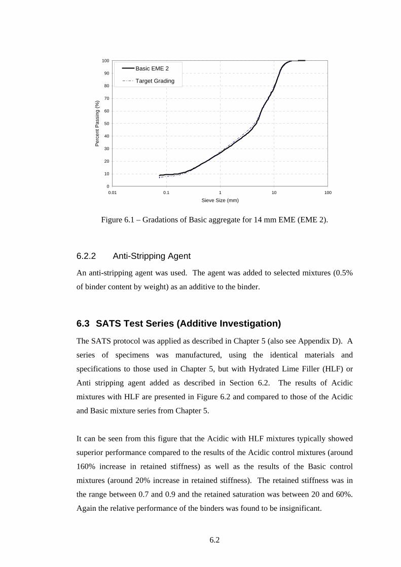
6.2

0

10

20

30

40

50

60

70

80

90

100

0.01 0.1 1 10 100

Sieve Size (mm)

Perc

ent P

assi

ng (%

)

Basic EME 2

Target Grading

Figure 6.1 – Gradations of Basic aggregate for 14 mm EME (EME 2).

6.2.2 Anti-Stripping Agent

An anti-stripping agent was used. The agent was added to selected mixtures (0.5%

of binder content by weight) as an additive to the binder.

6.3 SATS Test Series (Additive Investigation)

The SATS protocol was applied as described in Chapter 5 (also see Appendix D). A

series of specimens was manufactured, using the identical materials and

specifications to those used in Chapter 5, but with Hydrated Lime Filler (HLF) or

Anti stripping agent added as described in Section 6.2. The results of Acidic

mixtures with HLF are presented in Figure 6.2 and compared to those of the Acidic

and Basic mixture series from Chapter 5.

It can be seen from this figure that the Acidic with HLF mixtures typically showed

superior performance compared to the results of the Acidic control mixtures (around

160% increase in retained stiffness) as well as the results of the Basic control

mixtures (around 20% increase in retained stiffness). The retained stiffness was in

the range between 0.7 and 0.9 and the retained saturation was between 20 and 60%.

Again the relative performance of the binders was found to be insignificant.

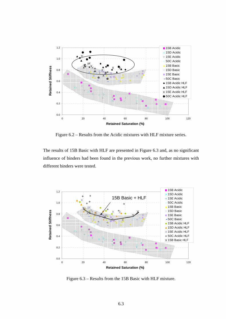
6.3

Figure 6.2 – Results from the Acidic mixtures with HLF mixture series.

The results of 15B Basic with HLF are presented in Figure 6.3 and, as no significant

influence of binders had been found in the previous work, no further mixtures with

different binders were tested.

Figure 6.3 – Results from the 15B Basic with HLF mixture.

0.0

0.2

0.4

0.6

0.8

1.0

1.2

0 20 40 60 80 100 120

Retained Saturation (%)

Ret

aine

d St

iffne

ss15B Acidic15D Acidic15E Acidic50C Acidic15B Basic15D Basic15E Basic50C Basic15B Acidic HLF15D Acidic HLF15E Acidic HLF50C Acidic HLF

0.0

0.2

0.4

0.6

0.8

1.0

1.2

0 20 40 60 80 100 120

Retained Saturation (%)

Ret

aine

d St

iffne

ss

15B Acidic15D Acidic15E Acidic50C Acidic15B Basic15D Basic15E Basic50C Basic15B Acidic HLF15D Acidic HLF15E Acidic HLF50C Acidic HLF15B Basic HLF

15B Basic + HLF

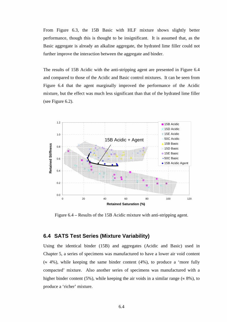
6.4

From Figure 6.3, the 15B Basic with HLF mixture shows slightly better

performance, though this is thought to be insignificant. It is assumed that, as the

Basic aggregate is already an alkaline aggregate, the hydrated lime filler could not

further improve the interaction between the aggregate and binder.

The results of 15B Acidic with the anti-stripping agent are presented in Figure 6.4

and compared to those of the Acidic and Basic control mixtures. It can be seen from

Figure 6.4 that the agent marginally improved the performance of the Acidic

mixture, but the effect was much less significant than that of the hydrated lime filler

(see Figure 6.2).

Figure 6.4 – Results of the 15B Acidic mixture with anti-stripping agent.

6.4 SATS Test Series (Mixture Variability)

Using the identical binder (15B) and aggregates (Acidic and Basic) used in

Chapter 5, a series of specimens was manufactured to have a lower air void content

(≈ 4%), while keeping the same binder content (4%), to produce a ‘more fully

compacted’ mixture. Also another series of specimens was manufactured with a

higher binder content (5%), while keeping the air voids in a similar range (≈ 8%), to

produce a ‘richer’ mixture.

0.0

0.2

0.4

0.6

0.8

1.0

1.2

0 20 40 60 80 100 120

Retained Saturation (%)

Ret

aine

d St

iffne

ss

15B Acidic15D Acidic15E Acidic50C Acidic15B Basic15D Basic15E Basic50C Basic15B Acidic Agent

15B Acidic + Agent

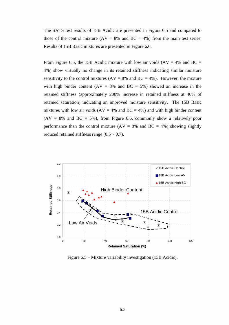
6.5

The SATS test results of 15B Acidic are presented in Figure 6.5 and compared to

those of the control mixture (AV = 8% and BC = 4%) from the main test series.

Results of 15B Basic mixtures are presented in Figure 6.6.

From Figure 6.5, the 15B Acidic mixture with low air voids (AV = 4% and BC =

4%) show virtually no change in its retained stiffness indicating similar moisture

sensitivity to the control mixtures (AV = 8% and BC = 4%). However, the mixture

with high binder content (AV = 8% and BC = 5%) showed an increase in the

retained stiffness (approximately 200% increase in retained stiffness at 40% of

retained saturation) indicating an improved moisture sensitivity. The 15B Basic

mixtures with low air voids (AV = 4% and BC = 4%) and with high binder content

(AV = 8% and BC = 5%), from Figure 6.6, commonly show a relatively poor

performance than the control mixture (AV = 8% and BC = 4%) showing slightly

reduced retained stiffness range (0.5 ~ 0.7).

Figure 6.5 – Mixture variability investigation (15B Acidic).

0.0

0.2

0.4

0.6

0.8

1.0

1.2

0 20 40 60 80 100 120

Retained Saturation (%)

Ret

aine

d St

iffne

ss

15B Acidic Control

15B Acidic Low AV

15B Acidic High BC

15B Acidic Control

Low Air Voids

High Binder Content

6.6

Figure 6.6 – Mixture variability investigation (15B Basic).

6.4.1 14 mm EME (EME 2)

A set of 14 mm EME (EME 2) specimens (AV = 4% and BC = 5.75%) was

manufactured using the 15E binder and Basic aggregate (see Section 6.2). The

SATS results are presented in Figure 6.7

0.0

0.2

0.4

0.6

0.8

1.0

1.2

0 20 40 60 80 100 120

Retained Saturation (%)

Ret

aine

d St

iffne

ss

15E Basic EME 2

Figure 6.7 – SATS test results of 15E Basic EME 2.

0.0

0.2

0.4

0.6

0.8

1.0

1.2

0 20 40 60 80 100 120

Retained Saturation (%)

Ret

aine

d St

iffne

ss

15B Basic Control

15B Basic Low AV

15B Basic High BC

15B Basic Control

High Binder Content Low Air Voids

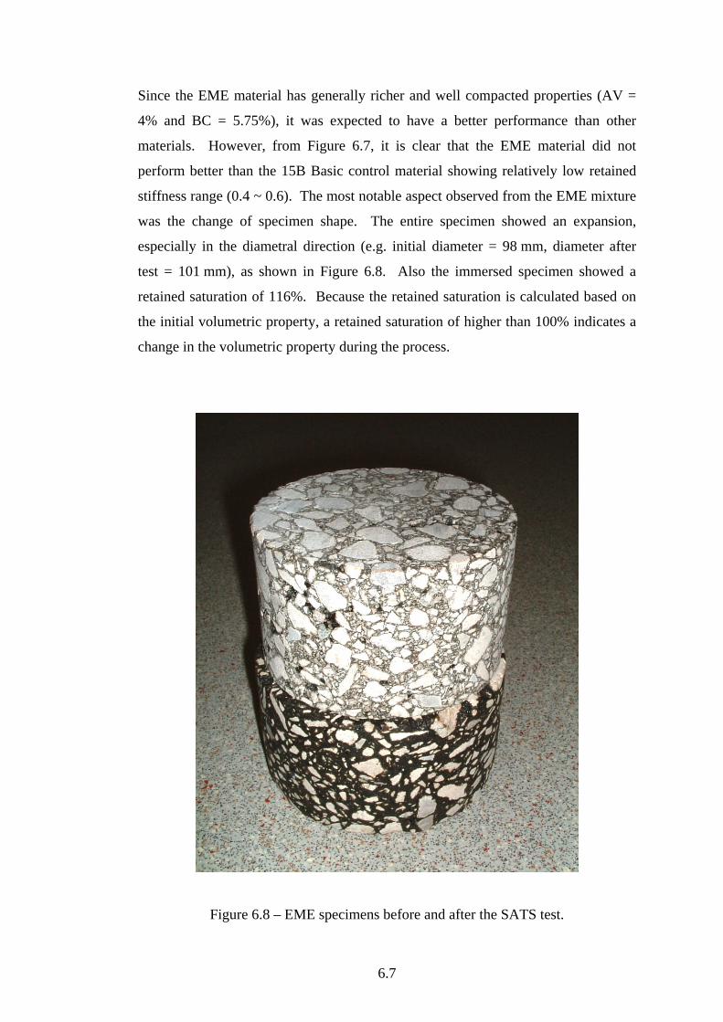
6.7

Since the EME material has generally richer and well compacted properties (AV =

4% and BC = 5.75%), it was expected to have a better performance than other

materials. However, from Figure 6.7, it is clear that the EME material did not

perform better than the 15B Basic control material showing relatively low retained

stiffness range (0.4 ~ 0.6). The most notable aspect observed from the EME mixture

was the change of specimen shape. The entire specimen showed an expansion,

especially in the diametral direction (e.g. initial diameter = 98 mm, diameter after

test = 101 mm), as shown in Figure 6.8. Also the immersed specimen showed a

retained saturation of 116%. Because the retained saturation is calculated based on

the initial volumetric property, a retained saturation of higher than 100% indicates a

change in the volumetric property during the process.

Figure 6.8 – EME specimens before and after the SATS test.

6.8

6.5 Summary and Conclusions

The SATS test was applied on a wider range of mixture conditions. Hydrated Lime

Filler (HLF) has generally been considered to improve the bonding interaction

between acidic aggregates and bituminous binders. The results from four Acidic

mixtures with HLF showed superior performances. The retained saturation range

(up to 60%) was also much reduced compared with both that of the Acidic control

mixture (up to 90%) and that of the Basic control mixture (up to 75%). It was

notable that some of the specimens with very low retained saturations (less than

25%) showed even higher retained stiffnesses than 1.0 (≈ 1.10). As with the Basic

mixtures, the immersed specimens commonly showed better performance than that

of the ‘non-immersed’ specimens, despite generally higher retained saturations.

The already good performance of the Basic control mixture was not significantly

improved by the adding of HLF. Only one binder (15B) was investigated for this

trial.

The effect of anti-stripping agent was investigated and showed an improved

performance, although it was found to be much less significant than that of hydrated

lime filler. However, it should be noted that the dosage of anti-stripping agent (0.5%

by weight of binder) was considerably low compared to the dosage of the hydrated

lime filler (2% by weight of aggregate), and a greater effect may be expected with a

higher dosage. Only one binder (15B) was used for this trial.

The investigation on mixture variability demonstrated an unexpected result where

the well compacted (lower air voids of 4%) or the richer mixture (higher binder

content of 5%) showed worse performance than the control mixture, especially for

the Basic mixtures. 15E EME Basic material also showed worse performance than

expected. Moreover, it clearly showed a volumetric expansion having a retained

saturation of higher than 100%.

An assumption was made that the specimen is damage/affected by another factor

together with the ageing and moisture factors in the vessel, and the richer and/or well

compacted mixture is considered to be more susceptible to the factor. The following

6.9

chapter presents a series of investigation to understand material behaviour and effect

of controlling factors of the SATS protocol.

7.1

Chapter 7. SATS Parameter Investigation

7.1 Review of SATS Protocol

The SATS protocol was developed based on the specific aim to develop a long-term

durability test protocol which can combine the binder ageing together with the

moisture sensitivity test. The SATS main test series, as described in Chapter 5, and

the recovered binder investigation (see Section 3.3) indicate that the SATS protocol

successfully fulfils the main objectives of this study. More specifically, the SATS

protocol could reproduce the given target stiffness modulus reduction (i.e. around

60% reduction, retained stiffness of 0.4) within a practically reasonable time scale

(65 hours). Also, within the very same process, the SATS protocol could age the

binder in the mixture comparable to the HiPAT binder ageing protocol which is

considered to be 10 or more years of long-term ageing process [Hayton et al., 1999].

However, the SATS test was mainly focused on the High Modulus Base material

with a relatively low binder content (≈ 4%) and a relatively high air void content (≈

8%). Extended application of SATS to various types of mixtures (see Chapter 6)

indicated that richer and/or well compacted mixtures were damage/affected by

another factor, not only by ageing and moisture damage, showing some unexpected

results. Therefore the following sections described a further investigation and

modification on the key factors (e.g. pressure, temperature and test duration etc) of

SATS protocol.

7.2 Test Setup

7.2.1 Temperature variation

The temperature inside of the pressure vessel was measured with partially filled

water as seen in Figure 5.3 and compared to those from the early trial (from Section

4.3.1) in Table 7.1. Figure 7.1 shows the measured temperature at each specimen

position.

7.2

Table 7.1 – Temperature variations of each SATS setup.

Target temperature of 85oC Max Temp. (oC)

Min Temp. (oC)

Variation (oC)

Normal setup (from Table 4.1) 90 77 13

Insulation on top cover (from Table 4.1) 86 80 6

Side heating source only (+ insulation on top cover) (from Table 4.1)

86 82 4

SATS (insulation applied as shown in Figure 4.6 (b)) 87 82 5

SATS (cover insulation removed) 87 80 7

Figure 7.1 – Measured temperatures at each specimen position (SATS).

As seen in Table 7.1 and Figure 7.1, the temperature variation of the standard SATS

protocol used in Chapter 5 was found to be around 5oC. However, it should be noted

that the maximum temperature was found at just below the water surface (between

4th and 5th specimens in Figure 5.3) where no specimen was used. Also the

temperature difference among the partially saturated specimens (Positions 1 ~ 4) as

found to be much less (around 2oC). It is noted that the insulation applied in SATS

(see Figure 4.6 (b)) appears to reduce the temperature variation up to 2oC, which is

comparable to the 7oC reduction observed in the preliminary setup (see Table 7.1).

Water level

0

1

2

3

4

5

6

777 79 81 83 85 87 89

Temperature (oC)

Spec

imen

Pos

ition

No Top Insulation

SATS setup

7.3

This difference is because that the temperature controlling thermocouple of the

vessel could make direct contact with the partially filled water (see Figure 7.2) which

results in a better temperature control (due to a better thermal conductivity of water)

confirming the suitability of the standard SATS setup for the vessel design.

Figure 7.2 – Standard SATS setup in the pressure vessel.

7.2.2 Tray design

A new tray was designed and manufactured to have larger holes in each specimen

shelf. This is to give a more increased and consistent water supply to the top

specimen and eventually to lower specimens. As seen in Figure 7.3, the new tray has

about five times larger hole area (φ 5 mm, 36 holes) than the old tray (φ 2 mm,

49 holes). Also the height of the empty space (between 4th and 5th specimens) has

been reduced to 45 mm.

Figure 7.4 shows a comparison of the new tray results to the old tray results using

the control mixtures (15B Acidic and 15B Basic). Both results are also compared to

the previous data from Chapter 5 where identical mixtures were tested for

repeatability (from Figure 5.7). As the results from both trays showed no significant

difference, the new tray shown in Figure 7.3 has been adopted for the further study.

Evaporation

Partially filled with Water

Dripping Water

Thermocouple

7.4

Figure 7.3 – Schematic and dimensions of the new specimen tray.

0.0

0.2

0.4

0.6

0.8

1.0

1.2

0 20 40 60 80 100 120

Retained Saturation (%)

Ret

aine

d St

iffne

ss

15B Acidic Control15B Basic Control15B Acidic - Old tray15B Basic - Old tray15B Acidic - New tray15B Basic - New tray

Figure 7.4 – Comparison of SATS results using old/new tray.

70 mm

70 mm

70 mm

70 mm

70 mm

45 mm

φ 8 mm, (Stainless steel)

φ 5 mm holes, evenly spaced (6 × 6 = 36 holes)

100 mm Square

2 mm Thickness plate (Stainless steel) 17 ± 2 mm

7.5

7.3 Pressure Condition

7.3.1 Half pressure SATS (1.0 MPa, 85oC, 65 hrs)

The most critical parameter of the SATS protocol is the applied pressure. The

pressure is the key parameter to accelerate the binder oxidation (ageing) process

through an increase amount of air and increased rate of diffusion. However, as the

SATS protocol is applied on compacted specimen, the effect of this high pressure on

the compacted specimen needs to be investigated. As the first step, the pressure

applied to the SATS protocol was halved to 1.0 MPa, while other parameters

remained the same. Both old and new trays were tested and results are presented in

Figure 7.5.

0.0

0.2

0.4

0.6

0.8

1.0

1.2

0 20 40 60 80 100 120

Retained Saturation (%)

Ret

aine

d St

iffne

ss

15B Acidic Control15B Basic Control15B Acidic - HP - OT15B Basic - HP - OT15B Acidic - HP - NT15B Basic - HP - NT

Figure 7.5 – Results of Half pressure SATS (1.0 MPa).

From Equation 5.3, it is clear that the specific humidity linearly increases as the

pressure decreases (i.e. ω ∝ P-1). Thus the reduced pressure will increase the amount

of water vapour inside the vessel which will result in an increased amount of

condensation beneath the lid, under the same temperature setup. Consequently, in a

tightly concealed environment, a more accelerated water circulation (increased

amount of dripping water supply to the specimens) is expected due to the increased

amount of condensation.

7.6

In Figure 7.5 results show, as expected, generally higher retained saturations from

most of the specimens (positions 1 ~ 4) with similar range of retained stiffnesses

compared to the full pressure (standard SATS) test results. It is noted that a higher

retained saturation range (50 ~ 85%) was found from 15B Basic with the new tray

results. An investigation on recovered binders revealed that the level of ageing from

the half pressure SATS is relatively lower than that from the full pressure test. More

details are found in Chapter 9 (Section 9.4.4).

7.3.2 Atmospheric SATS (No added pressure, 85oC, 65 hrs)

This is to perform the SATS protocol in atmospheric pressure condition. No

additional pressure was applied to the SATS protocol, while other parameters

remained the same. Results are presented in Figure 7.6.

0.0

0.2

0.4

0.6

0.8

1.0

1.2

0 20 40 60 80 100 120

Retained Saturation (%)

Ret

aine

d St

iffne

ss

15B Acidic control15B Basic control15B Acidic - New tray15B Basic - New tray15B Acidic - NT - AP15B Basic - NT - AP

Figure 7.6 – Results of Atmospheric SATS.

From Figure 7.6, 15B Acidic shows generally higher retained saturation (over 60%)

from most of the specimens (positions 1 ~ 4) with similar levels of retained stiffness

(less than 0.3). However, the 15B Basic showed a similar range of retained

saturation with virtually no reduction in the retained stiffness (0.9 ~ 1.0).

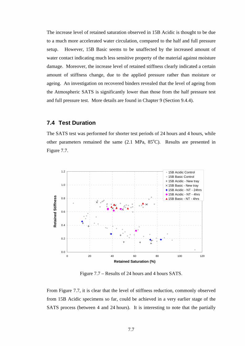
7.7

The increase level of retained saturation observed in 15B Acidic is thought to be due

to a much more accelerated water circulation, compared to the half and full pressure

setup. However, 15B Basic seems to be unaffected by the increased amount of

water contact indicating much less sensitive property of the material against moisture

damage. Moreover, the increase level of retained stiffness clearly indicated a certain

amount of stiffness change, due to the applied pressure rather than moisture or

ageing. An investigation on recovered binders revealed that the level of ageing from

the Atmospheric SATS is significantly lower than those from the half pressure test

and full pressure test. More details are found in Chapter 9 (Section 9.4.4).

7.4 Test Duration

The SATS test was performed for shorter test periods of 24 hours and 4 hours, while

other parameters remained the same (2.1 MPa, 85oC). Results are presented in

Figure 7.7.

0.0

0.2

0.4

0.6

0.8

1.0

1.2

0 20 40 60 80 100 120

Retained Saturation (%)

Ret

aine

d St

iffne

ss

15B Acidic Control15B Basic Control15B Acidic - New tray15B Basic - New tray15B Acidic - NT - 24hrs15B Acidic - NT - 4hrs15B Basic - NT - 4hrs

Figure 7.7 – Results of 24 hours and 4 hours SATS.

From Figure 7.7, it is clear that the level of stiffness reduction, commonly observed

from 15B Acidic specimens so far, could be achieved in a very earlier stage of the

SATS process (between 4 and 24 hours). It is interesting to note that the partially

7.8

saturated specimens (positions 1 ~ 4) from 4 hours SATS showed a very narrow

range of retained saturation (around 40%) which is even lower than the initial

saturation measured after the vacuum process (around 60%).

It can be assumed that, once the vacuum saturated specimens are placed in the

vessel, a certain proportion of the initially saturated water (by the vacuum process) is

commonly drained out of the specimens (above the water level, positions 1 ~ 4)

resulting in a bit lower range of retained saturation than the initial saturation, as

observed in ‘4 hours SATS’ results. However, the condensed water from the lid

starts to gradually re-saturate the specimens (from the top specimen) and, therefore

results in the observed the retained saturation variation along the specimen position

so far. The condensed water appears to re-saturate the specimens from around 4

hours after the process starts, and also this gradual re-saturation process appears to

be stabilised within approximately 24 hours period. Thus the observed retained

saturation variation of each specimen assumed to be maintained from around

24 hours to the completion of the test (65 hours).

Also it can be concluded that the observed retained saturation variation along the

specimen position is mainly created by the dripping condensed water, rather than the

initially saturated water, supporting the theory proposed in Section 5.5.2. 15B Basic

specimens showed similar results to the full period SATS (standard SATS). An

investigation on recovered binders revealed that the levels of ageing from the shorter

period SATS tests are relatively lower than that from the full period SATS. More

details are found in Chapter 9 (Section 9.4.5).

7.5 Temperature Condition

The SATS test was performed using lower temperatures of 60oC and 30oC, while

other parameters remained the same (2.1 MPa, 65 hrs). Results are presented in

Figure 7.8.

From Figure 7.8, the 15B Acidic specimens show a close relation to the applied

temperatures. The results from 60oC SATS show an increased retained stiffness

range (0.5 to 0.7), including the immersed specimen (Position 6), with a generally

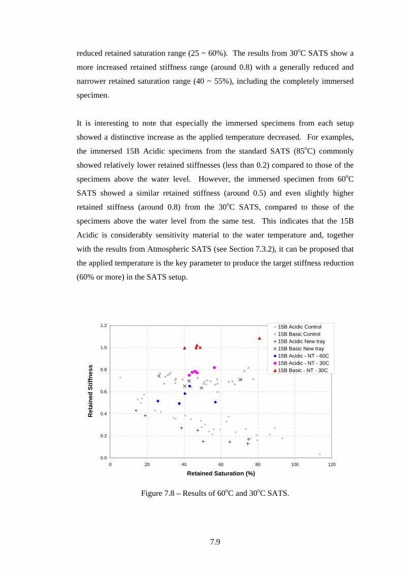
7.9

reduced retained saturation range (25 ~ 60%). The results from 30oC SATS show a

more increased retained stiffness range (around 0.8) with a generally reduced and

narrower retained saturation range (40 ~ 55%), including the completely immersed

specimen.

It is interesting to note that especially the immersed specimens from each setup

showed a distinctive increase as the applied temperature decreased. For examples,

the immersed 15B Acidic specimens from the standard SATS (85oC) commonly

showed relatively lower retained stiffnesses (less than 0.2) compared to those of the

specimens above the water level. However, the immersed specimen from 60oC

SATS showed a similar retained stiffness (around 0.5) and even slightly higher

retained stiffness (around 0.8) from the 30oC SATS, compared to those of the

specimens above the water level from the same test. This indicates that the 15B

Acidic is considerably sensitivity material to the water temperature and, together

with the results from Atmospheric SATS (see Section 7.3.2), it can be proposed that

the applied temperature is the key parameter to produce the target stiffness reduction

(60% or more) in the SATS setup.

0.0

0.2

0.4

0.6

0.8

1.0

1.2

0 20 40 60 80 100 120

Retained Saturation (%)

Ret

aine

d St

iffne

ss

15B Acidic Control15B Basic Control15B Acidic New tray15B Basic New tray15B Acidic - NT - 60C15B Acidic - NT - 30C15B Basic - NT - 30C

Figure 7.8 – Results of 60oC and 30oC SATS.

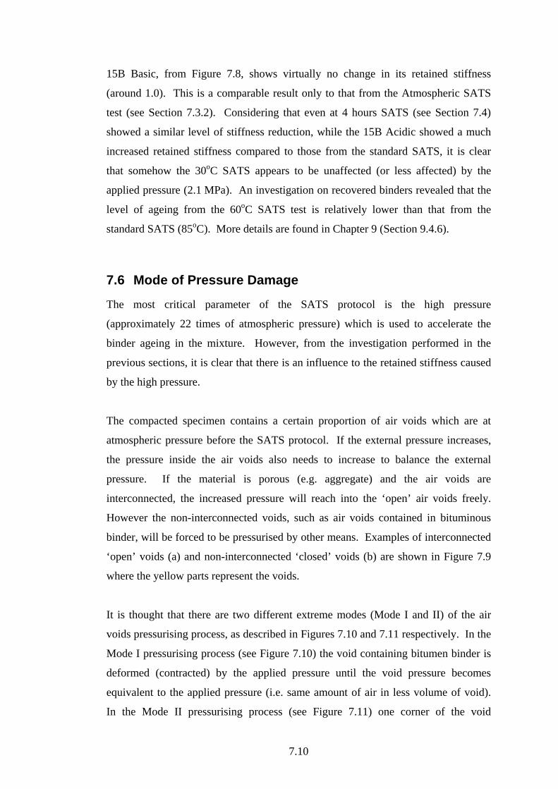
7.10

15B Basic, from Figure 7.8, shows virtually no change in its retained stiffness

(around 1.0). This is a comparable result only to that from the Atmospheric SATS

test (see Section 7.3.2). Considering that even at 4 hours SATS (see Section 7.4)

showed a similar level of stiffness reduction, while the 15B Acidic showed a much

increased retained stiffness compared to those from the standard SATS, it is clear

that somehow the 30oC SATS appears to be unaffected (or less affected) by the

applied pressure (2.1 MPa). An investigation on recovered binders revealed that the

level of ageing from the 60oC SATS test is relatively lower than that from the

standard SATS (85oC). More details are found in Chapter 9 (Section 9.4.6).

7.6 Mode of Pressure Damage

The most critical parameter of the SATS protocol is the high pressure

(approximately 22 times of atmospheric pressure) which is used to accelerate the

binder ageing in the mixture. However, from the investigation performed in the

previous sections, it is clear that there is an influence to the retained stiffness caused

by the high pressure.

The compacted specimen contains a certain proportion of air voids which are at

atmospheric pressure before the SATS protocol. If the external pressure increases,

the pressure inside the air voids also needs to increase to balance the external

pressure. If the material is porous (e.g. aggregate) and the air voids are

interconnected, the increased pressure will reach into the ‘open’ air voids freely.

However the non-interconnected voids, such as air voids contained in bituminous

binder, will be forced to be pressurised by other means. Examples of interconnected

‘open’ voids (a) and non-interconnected ‘closed’ voids (b) are shown in Figure 7.9

where the yellow parts represent the voids.

It is thought that there are two different extreme modes (Mode I and II) of the air

voids pressurising process, as described in Figures 7.10 and 7.11 respectively. In the

Mode I pressurising process (see Figure 7.10) the void containing bitumen binder is

deformed (contracted) by the applied pressure until the void pressure becomes

equivalent to the applied pressure (i.e. same amount of air in less volume of void).

In the Mode II pressurising process (see Figure 7.11) one corner of the void

7.11

containing bitumen binder is ‘punctured’ providing a ‘channel’ for the pressurised

air to infiltrate into the void, until becomes equivalent to the applied pressure (i.e.

more amount of air in same volume of void). These processes are also likely to be

taking place when the pressure is released (depressurising process) after the SATS

protocol, in a reverse manner. For examples, in Mode I depressurising process, the

air void containing binder will ‘expand’ to equalise the decreasing external pressure

(same amount of air in more volume of void), while the pressure will be released

through the pressure channel (puncture) in Mode II depressurising process.

(a) Interconnected air voids (b) Non-interconnected air voids

Figure 7.9 – Examples of interconnected air voids and non-interconnected air voids in a ‘compacted’ bituminous mixture.

Figure 7.10 – Conceptual diagram of Mode I (deformation) void pressurising process.

Applied pressure

Air voids (Atmospheric pressure)

Binder (Air tight)

Pressurising

Air voids (= Applied pressure)

7.12

Figure 7.11 – Conceptual diagram of Mode II (puncture) void pressurising process.

The ‘punctures’ created in Mode II process are thought to be microscopic and the

volumetric change is none (or minimal), giving minimum disturbance to the

surrounding aggregate structure (see Figure 7.12). However, in Mode I

depressurising process, the affected (deformed) area (or volume) of the binder is

much greater (all around the void) giving maximum disturbance to the surrounding

aggregate structure, due to the physical expansion of the void containing binder (see

Figure 7.13). Therefore a physical damage to the compacted specimen, caused by

the pressurising or depressurising process, is thought to be far greater in Mode I than

Mode II.

It is logical to think that, considering the visco-elastic and temperature dependent

characteristics of bituminous binder, the Mode I process is more likely to happen

when the binder is in higher temperature having more viscous property, whereas the

Mode II is more likely in the lower temperature with more elastic property.

However in reality, as the above assumptions were made for the extreme cases, both

modes of pressurising (or depressurising) process are likely happening together. A

specimen, as an example, could be damaged by the Mode I process up to a certain

proportion then move on to Mode II process. At a higher temperature Mode I

damage is considered to be a dominant form but there will still be a minor proportion

of Mode II damage and vice versa for the lower temperature case.

Air voids (Atmospheric pressure)

Binder (Air tight)

Pressurising

Air voids (= Applied pressure)

Puncture (Pressure channel) Applied

pressure

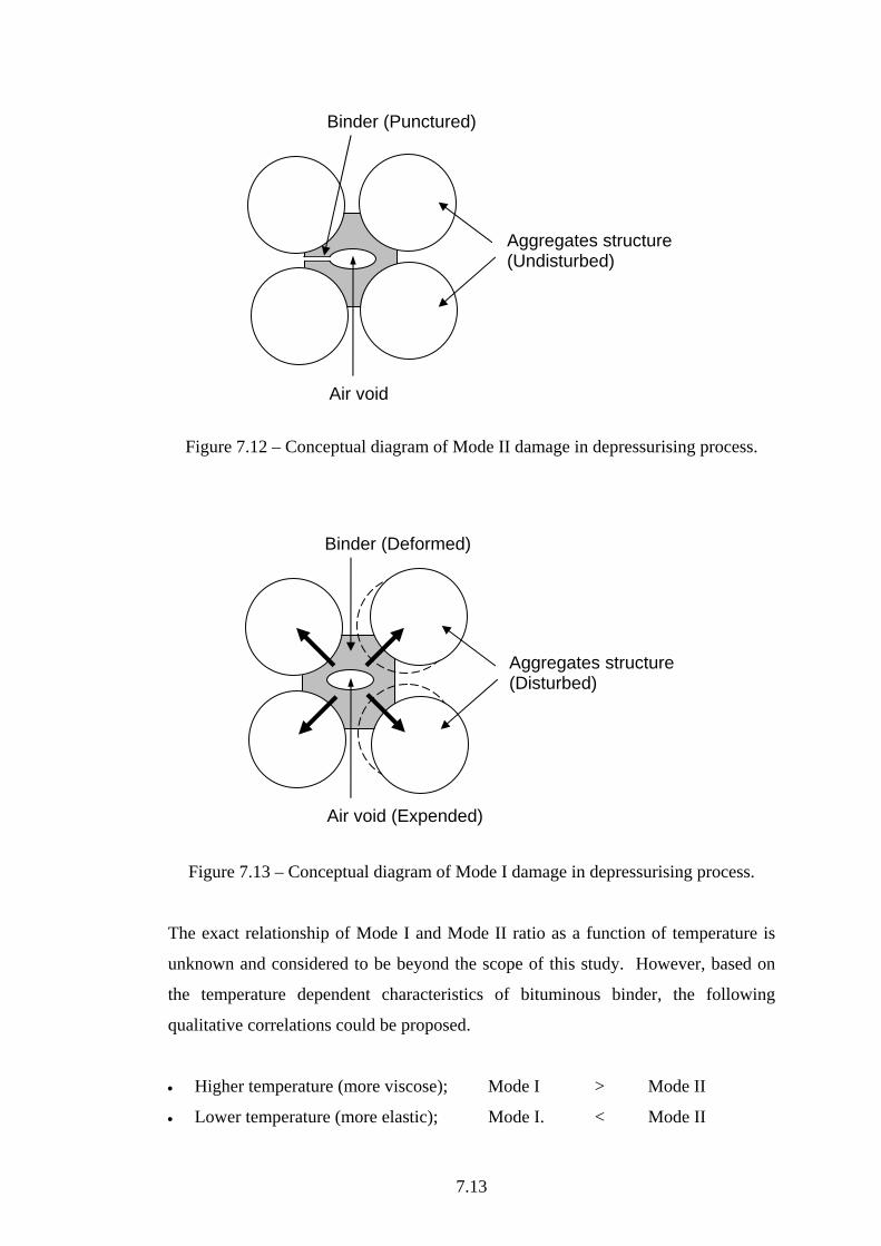
7.13

Figure 7.12 – Conceptual diagram of Mode II damage in depressurising process.

Figure 7.13 – Conceptual diagram of Mode I damage in depressurising process.

The exact relationship of Mode I and Mode II ratio as a function of temperature is

unknown and considered to be beyond the scope of this study. However, based on

the temperature dependent characteristics of bituminous binder, the following

qualitative correlations could be proposed.

• Higher temperature (more viscose); Mode I > Mode II

• Lower temperature (more elastic); Mode I. < Mode II

Air void

Binder (Punctured)

Aggregates structure (Undisturbed)

Air void (Expended)

Binder (Deformed)

Aggregates structure (Disturbed)

7.14

Also at a same temperature;

• High pen grade binder (more viscose); Mode I > Mode II

• Low pen grade binder (more elastic); Mode I < Mode II

7.7 Summary and Conclusions

The developed ‘standard SATS’ protocol appears to fulfil the main objectives of the

study, providing a durability test protocol which combines long-term binder ageing

process and mixture moisture sensitivity process. However, from a further

investigation on the parameters used in the protocol (i.e. pressure, temperature and

test duration) it appears that the high pressure (introduced to accelerate binder ageing

process) also induces a certain degree of specimen damage. Consequently two

different modes of pressure related damage have been proposed and their expected

properties are suggested.

Assuming that only bitumen binder is likely to be affected by the pressuring/

depressurising process, a mixture with a more binder content and/or low air voids

content is thought to be more susceptible to the pressurising/depressurising damage

from the SATS protocol, since the mixture is likely to have a more closed ‘non-

interconnected’ voids. Also, a mixture with a better adhesion property between

aggregates and binder will be more susceptible to the pressurising/depressurising

damage as the mixture will create more ‘non-interconnected’ voids along the

interface of aggregate and binder.

The following chapter describes an investigation to prevent (or minimise) the

pressure related damage discussed in this chapter.

8.1

Chapter 8. SATS Modification

8.1 Review of Pressure Damage

Investigation from Chapter 7 clearly indicated that there is a certain degree of

damage (i.e. reduction in retained stiffness) caused by the pressure used in the SATS

protocol. Thus the unexpected results observed in Chapter 6 are thought to be due to

the influence of pressure related damage. Especially the 15E EME Basic mixture

(see Section 6.4.1) is considered to be most affected by the pressure damage,

showing unexpectedly low retained stiffnesses (around 0.5) with a clearly visible

shape change (diametral expansion). It should be note that the 15E EME mixture

has the highest binder content (5.75%), the lowest air voids (4%) and the smallest

maximum aggregates size (14 mm, compared to 28 mm DBM) which overall could

contribute to produce a considerably more ‘pressure sensitive’ specimen (containing

much more ‘non-interconnected’ air voids).

The following sections describe further modifications to the standard SATS protocol

with the principal objective to remove (or reduce) the pressure related damage.

8.2 Depressurising Process Investigation

The pressure damage appears to be more related to the pressurising or depressurising

process, rather than the absolute value of the applied pressure, since the 15B Basic

specimens from the half pressure SATS (see Section 7.3.1) and the full pressure

standard SATS showed a very similar retained stiffness range. In the standard SATS

protocol (see Appendix D), the pressurising process takes place when the specimens

are still in ambient temperature, since the pressure is applied during the first

20 minutes, immediately after the specimens are placed in the vessel following the

vacuum saturation process in ambient temperature (≈ 20oC). However the

depressurising process takes place when the specimens are fully heated (≈ 85oC).

The study in Section 7.6 has suggested that the specimens are likely more susceptible

to the pressure damage at a higher temperature (as Mode I damage is dominant), thus

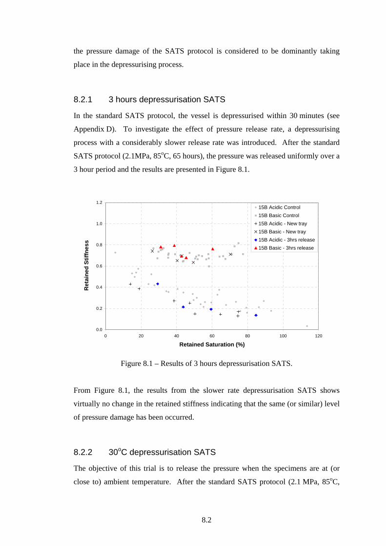
8.2

the pressure damage of the SATS protocol is considered to be dominantly taking

place in the depressurising process.

8.2.1 3 hours depressurisation SATS

In the standard SATS protocol, the vessel is depressurised within 30 minutes (see

Appendix D). To investigate the effect of pressure release rate, a depressurising

process with a considerably slower release rate was introduced. After the standard

SATS protocol (2.1MPa, 85oC, 65 hours), the pressure was released uniformly over a

3 hour period and the results are presented in Figure 8.1.

0.0

0.2

0.4

0.6

0.8

1.0

1.2

0 20 40 60 80 100 120

Retained Saturation (%)

Ret

aine

d St

iffne

ss

15B Acidic Control15B Basic Control15B Acidic - New tray15B Basic - New tray15B Acidic - 3hrs release15B Basic - 3hrs release

Figure 8.1 – Results of 3 hours depressurisation SATS.

From Figure 8.1, the results from the slower rate depressurisation SATS shows

virtually no change in the retained stiffness indicating that the same (or similar) level

of pressure damage has been occurred.

8.2.2 30oC depressurisation SATS

The objective of this trial is to release the pressure when the specimens are at (or

close to) ambient temperature. After the standard SATS protocol (2.1 MPa, 85oC,

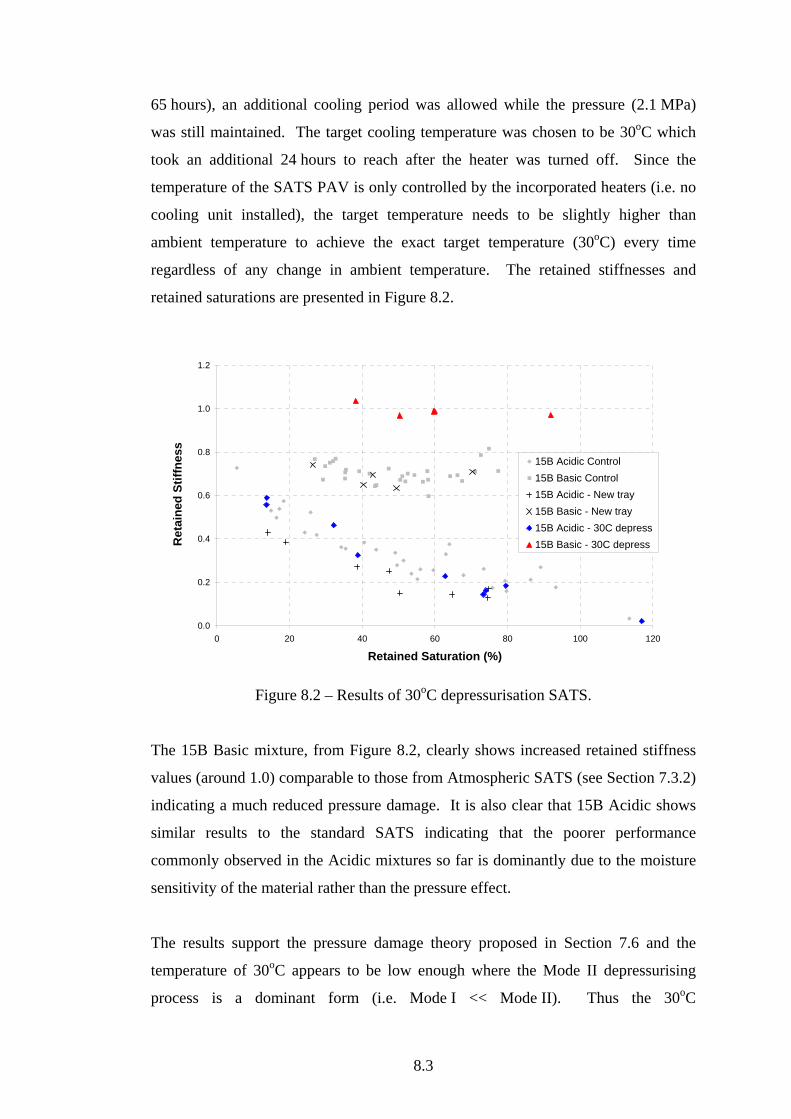
8.3

65 hours), an additional cooling period was allowed while the pressure (2.1 MPa)

was still maintained. The target cooling temperature was chosen to be 30oC which

took an additional 24 hours to reach after the heater was turned off. Since the

temperature of the SATS PAV is only controlled by the incorporated heaters (i.e. no

cooling unit installed), the target temperature needs to be slightly higher than

ambient temperature to achieve the exact target temperature (30oC) every time

regardless of any change in ambient temperature. The retained stiffnesses and

retained saturations are presented in Figure 8.2.

0.0

0.2

0.4

0.6

0.8

1.0

1.2

0 20 40 60 80 100 120

Retained Saturation (%)

Ret

aine

d St

iffne

ss

15B Acidic Control15B Basic Control15B Acidic - New tray15B Basic - New tray15B Acidic - 30C depress15B Basic - 30C depress

Figure 8.2 – Results of 30oC depressurisation SATS.

The 15B Basic mixture, from Figure 8.2, clearly shows increased retained stiffness

values (around 1.0) comparable to those from Atmospheric SATS (see Section 7.3.2)

indicating a much reduced pressure damage. It is also clear that 15B Acidic shows

similar results to the standard SATS indicating that the poorer performance

commonly observed in the Acidic mixtures so far is dominantly due to the moisture

sensitivity of the material rather than the pressure effect.

The results support the pressure damage theory proposed in Section 7.6 and the

temperature of 30oC appears to be low enough where the Mode II depressurising

process is a dominant form (i.e. Mode I << Mode II). Thus the 30oC

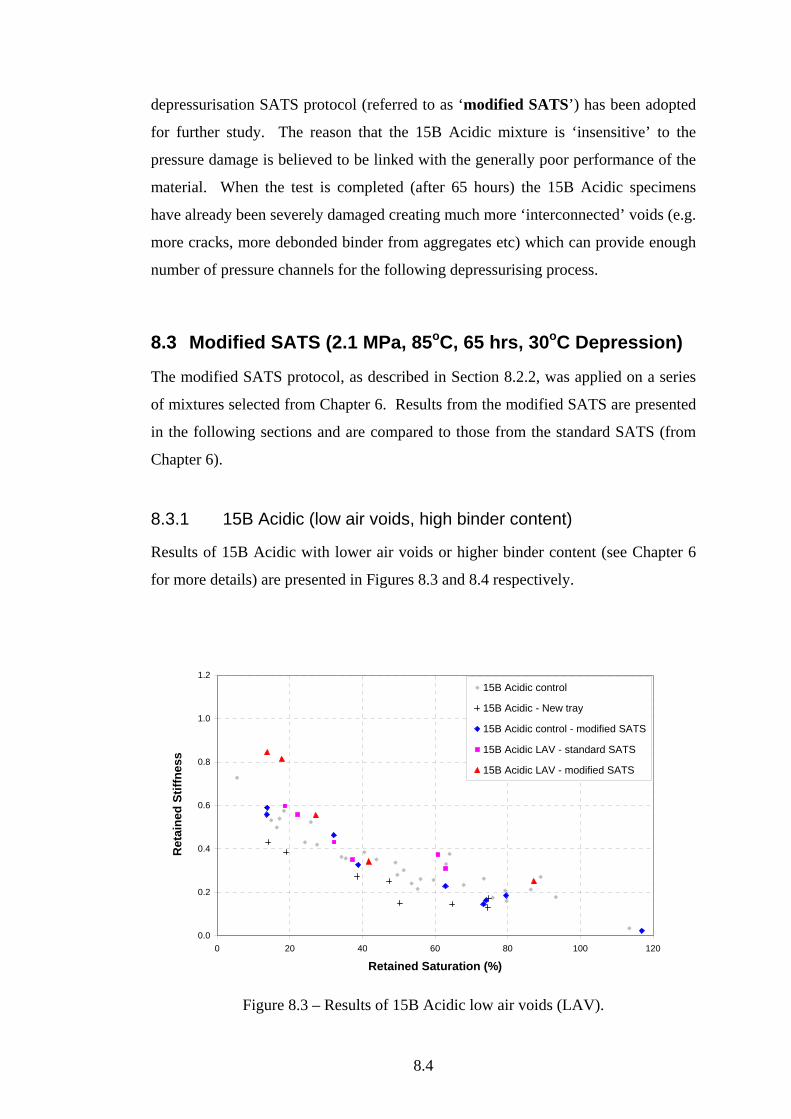
8.4

depressurisation SATS protocol (referred to as ‘modified SATS’) has been adopted

for further study. The reason that the 15B Acidic mixture is ‘insensitive’ to the

pressure damage is believed to be linked with the generally poor performance of the

material. When the test is completed (after 65 hours) the 15B Acidic specimens

have already been severely damaged creating much more ‘interconnected’ voids (e.g.

more cracks, more debonded binder from aggregates etc) which can provide enough

number of pressure channels for the following depressurising process.

8.3 Modified SATS (2.1 MPa, 85oC, 65 hrs, 30oC Depression)

The modified SATS protocol, as described in Section 8.2.2, was applied on a series

of mixtures selected from Chapter 6. Results from the modified SATS are presented

in the following sections and are compared to those from the standard SATS (from

Chapter 6).

8.3.1 15B Acidic (low air voids, high binder content)

Results of 15B Acidic with lower air voids or higher binder content (see Chapter 6

for more details) are presented in Figures 8.3 and 8.4 respectively.

0.0

0.2

0.4

0.6

0.8

1.0

1.2

0 20 40 60 80 100 120

Retained Saturation (%)

Ret

aine

d St

iffne

ss

15B Acidic control

15B Acidic - New tray

15B Acidic control - modified SATS

15B Acidic LAV - standard SATS

15B Acidic LAV - modified SATS

Figure 8.3 – Results of 15B Acidic low air voids (LAV).

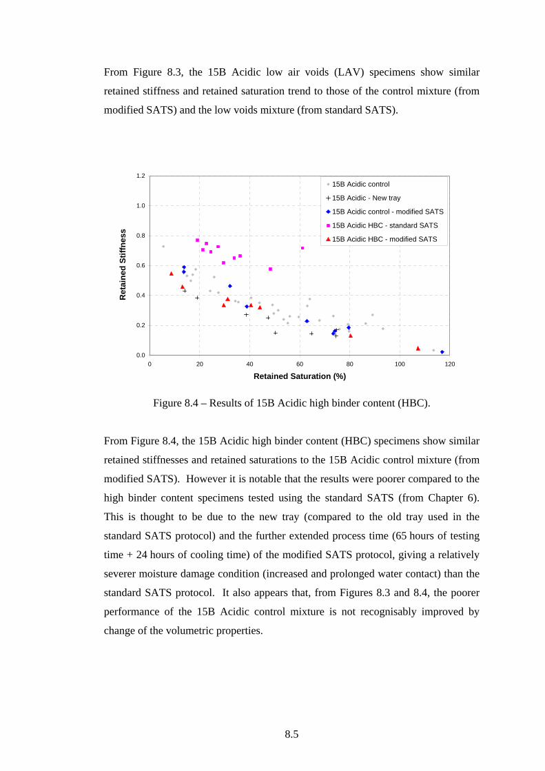
8.5

From Figure 8.3, the 15B Acidic low air voids (LAV) specimens show similar

retained stiffness and retained saturation trend to those of the control mixture (from

modified SATS) and the low voids mixture (from standard SATS).

0.0

0.2

0.4

0.6

0.8

1.0

1.2

0 20 40 60 80 100 120

Retained Saturation (%)

Ret

aine

d St

iffne

ss

15B Acidic control

15B Acidic - New tray

15B Acidic control - modified SATS

15B Acidic HBC - standard SATS

15B Acidic HBC - modified SATS

Figure 8.4 – Results of 15B Acidic high binder content (HBC).

From Figure 8.4, the 15B Acidic high binder content (HBC) specimens show similar

retained stiffnesses and retained saturations to the 15B Acidic control mixture (from

modified SATS). However it is notable that the results were poorer compared to the

high binder content specimens tested using the standard SATS (from Chapter 6).

This is thought to be due to the new tray (compared to the old tray used in the

standard SATS protocol) and the further extended process time (65 hours of testing

time + 24 hours of cooling time) of the modified SATS protocol, giving a relatively

severer moisture damage condition (increased and prolonged water contact) than the

standard SATS protocol. It also appears that, from Figures 8.3 and 8.4, the poorer

performance of the 15B Acidic control mixture is not recognisably improved by

change of the volumetric properties.

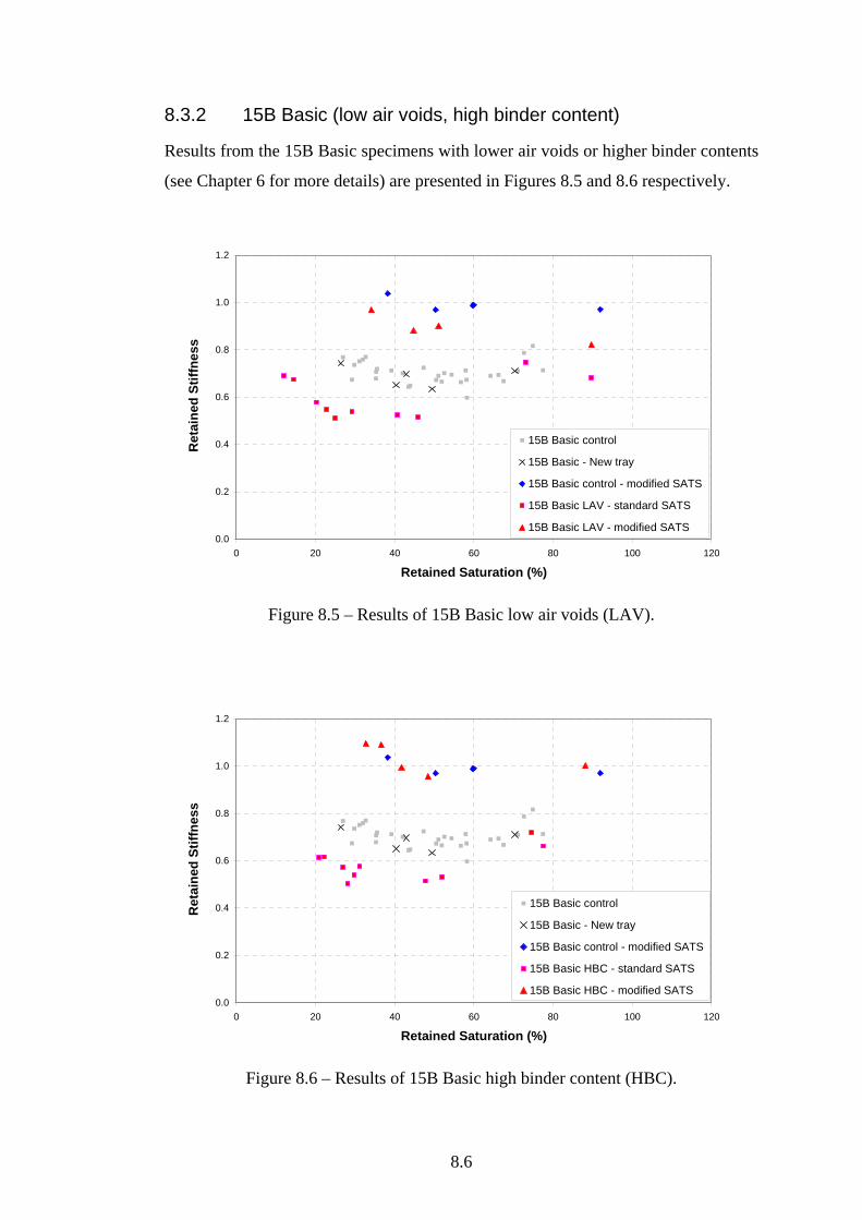
8.6

8.3.2 15B Basic (low air voids, high binder content)

Results from the 15B Basic specimens with lower air voids or higher binder contents

(see Chapter 6 for more details) are presented in Figures 8.5 and 8.6 respectively.

0.0

0.2

0.4

0.6

0.8

1.0

1.2

0 20 40 60 80 100 120

Retained Saturation (%)

Ret

aine

d St

iffne

ss

15B Basic control

15B Basic - New tray

15B Basic control - modified SATS

15B Basic LAV - standard SATS

15B Basic LAV - modified SATS

Figure 8.5 – Results of 15B Basic low air voids (LAV).

0.0

0.2

0.4

0.6

0.8

1.0

1.2

0 20 40 60 80 100 120

Retained Saturation (%)

Ret

aine

d St

iffne

ss

15B Basic control

15B Basic - New tray

15B Basic control - modified SATS

15B Basic HBC - standard SATS

15B Basic HBC - modified SATS

Figure 8.6 – Results of 15B Basic high binder content (HBC).

8.7

From Figures 8.5 and 8.6, the 15B Basic specimens with low air voids (LAV), or

high binder content (HBC), commonly show much increased retained stiffness

ranges, compared to those of the specimens tested using the standard SATS protocol

(from Chapter 6) indicating a much reduced pressure damage. Also both mixtures

commonly show comparable ranges of retained stiffnesses (LAV = 0.80 ~ 1.00,

HBC = 0.95 ~ 1.10) to the control mixture tested using the modified SATS protocol

(around 1.0). It is thought that the already well performing 15B Basic control

mixture is not significantly affected by the volumetric changes used in this study.

8.3.3 15E EME Basic

Results of 15E EME Basic (see Chapter 6 for more details) are presented in Figure

8.7.

0.0

0.2

0.4

0.6

0.8

1.0

1.2

0 20 40 60 80 100 120

Retained Saturation (%)

Ret

aine

d St

iffne

ss

15B Basic control

15B Basic - New tray

15B Basic control - modified SATS

15E EME Basic - standard SATS

15E EME Basic - modified SATS

Figure 8.7 – Results of 15E EME Basic.

From Figure 8.7, the 15E EME Basic specimens show a much increased retained

stiffness range (0.80 ~ 1.05, from specimens above water level), compared to that of

the specimens tested using the standard SATS protocol (around 0.5, from Chapter 6)

indicating a much reduced pressure damage. The visible swelling of the specimen

observed in Figure 6.8 also significantly reduced showing virtually no change in the

shape (see Figure 8.8 – (b)).

8.8

Since the 15E EME Basic mixture is thought to be more pressure sensitive, the

marginally lower range of retained stiffnesses than 15B Basic control mixture (see

Figure 8.7) is presumed to be due to a relatively higher level of pressure damage,

rather than its true moisture sensitivity.

(a) Standard SATS (from Figure 6.8) (b) Modified SATS

Figure 8.8 – Comparison of EME specimens before and after the SATS test (standard SATS and modified SATS).

It is notable that the immersed specimens (Position 6) typically showed a higher

retained stiffness than those from the non-immersed specimens (Positions 1 ~ 4)

which is also typically found from most of the Basic mixtures investigated in

Chapters 5, 6 and 7. It is thought that the ‘pressurised’ water confines all around the

specimen giving an extra support to the immersed specimen.

8.3.4 15B Acidic with HLF

Results of 15B Acidic with HLF (see Chapter 6 for more details) tested using the

modified SATS protocol are presented in Figure 8.9. The 15B Acidic HLF

specimens, from this figure, show a similar retained stiffness range (around 1.0)

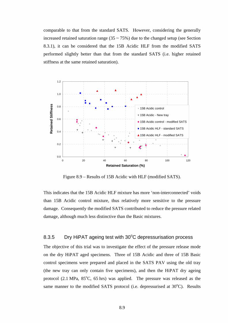
8.9

comparable to that from the standard SATS. However, considering the generally

increased retained saturation range (35 ~ 75%) due to the changed setup (see Section

8.3.1), it can be considered that the 15B Acidic HLF from the modified SATS

performed slightly better than that from the standard SATS (i.e. higher retained

stiffness at the same retained saturation).

0.0

0.2

0.4

0.6

0.8

1.0

1.2

0 20 40 60 80 100 120

Retained Saturation (%)

Ret

aine

d St

iffne

ss 15B Acidic control

15B Acidic - New tray

15B Acidic control - modified SATS

15B Acidic HLF - standard SATS

15B Acidic HLF - modified SATS

Figure 8.9 – Results of 15B Acidic with HLF (modified SATS).

This indicates that the 15B Acidic HLF mixture has more ‘non-interconnected’ voids

than 15B Acidic control mixture, thus relatively more sensitive to the pressure

damage. Consequently the modified SATS contributed to reduce the pressure related

damage, although much less distinctive than the Basic mixtures.

8.3.5 Dry HiPAT ageing test with 30oC depressurisation process

The objective of this trial was to investigate the effect of the pressure release mode

on the dry HiPAT aged specimens. Three of 15B Acidic and three of 15B Basic

control specimens were prepared and placed in the SATS PAV using the old tray

(the new tray can only contain five specimens), and then the HiPAT dry ageing

protocol (2.1 MPa, 85oC, 65 hrs) was applied. The pressure was released as the

same manner to the modified SATS protocol (i.e. depressurised at 30oC). Results

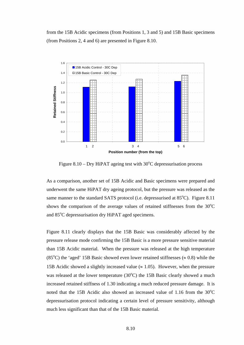
8.10

from the 15B Acidic specimens (from Positions 1, 3 and 5) and 15B Basic specimens

(from Positions 2, 4 and 6) are presented in Figure 8.10.

0.0

0.2

0.4

0.6

0.8

1.0

1.2

1.4

1.6

1 2 3 4 5 6

Position number (from the top)

Ret

aine

d St

iffne

ss

15B Acidic Control - 30C Dep

15B Basic Control - 30C Dep

Figure 8.10 – Dry HiPAT ageing test with 30oC depressurisation process

As a comparison, another set of 15B Acidic and Basic specimens were prepared and

underwent the same HiPAT dry ageing protocol, but the pressure was released as the

same manner to the standard SATS protocol (i.e. depressurised at 85oC). Figure 8.11

shows the comparison of the average values of retained stiffnesses from the 30oC

and 85oC depressurisation dry HiPAT aged specimens.

Figure 8.11 clearly displays that the 15B Basic was considerably affected by the

pressure release mode confirming the 15B Basic is a more pressure sensitive material

than 15B Acidic material. When the pressure was released at the high temperature

(85oC) the ‘aged’ 15B Basic showed even lower retained stiffnesses (≈ 0.8) while the

15B Acidic showed a slightly increased value (≈ 1.05). However, when the pressure

was released at the lower temperature (30oC) the 15B Basic clearly showed a much

increased retained stiffness of 1.30 indicating a much reduced pressure damage. It is

noted that the 15B Acidic also showed an increased value of 1.16 from the 30oC

depressurisation protocol indicating a certain level of pressure sensitivity, although

much less significant than that of the 15B Basic material.

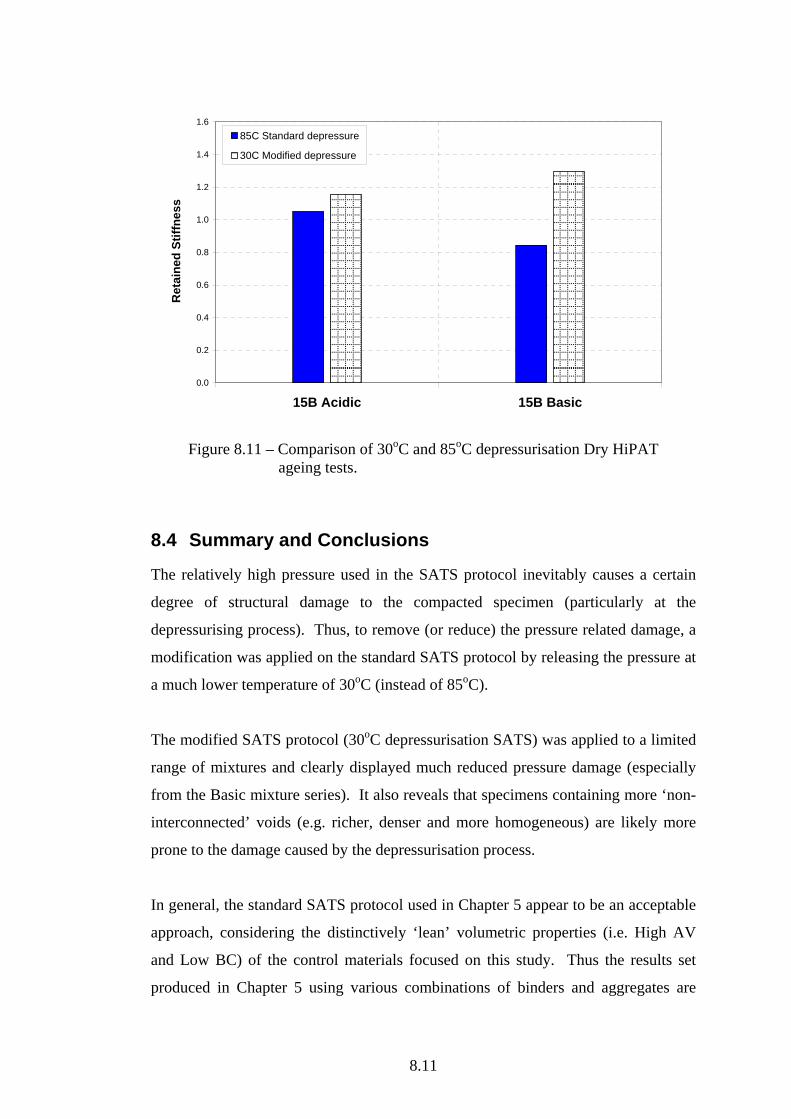
8.11

0.0

0.2

0.4

0.6

0.8

1.0

1.2

1.4

1.6

15B Acidic 15B Basic

Ret

aine

d St

iffne

ss

85C Standard depressure

30C Modified depressure

Figure 8.11 – Comparison of 30oC and 85oC depressurisation Dry HiPAT

ageing tests.

8.4 Summary and Conclusions

The relatively high pressure used in the SATS protocol inevitably causes a certain

degree of structural damage to the compacted specimen (particularly at the

depressurising process). Thus, to remove (or reduce) the pressure related damage, a

modification was applied on the standard SATS protocol by releasing the pressure at

a much lower temperature of 30oC (instead of 85oC).

The modified SATS protocol (30oC depressurisation SATS) was applied to a limited

range of mixtures and clearly displayed much reduced pressure damage (especially

from the Basic mixture series). It also reveals that specimens containing more ‘non-

interconnected’ voids (e.g. richer, denser and more homogeneous) are likely more

prone to the damage caused by the depressurisation process.

In general, the standard SATS protocol used in Chapter 5 appear to be an acceptable

approach, considering the distinctively ‘lean’ volumetric properties (i.e. High AV

and Low BC) of the control materials focused on this study. Thus the results set

produced in Chapter 5 using various combinations of binders and aggregates are

8.12

considered to be credible, especially for the Acidic materials which are nominally

identical to the HMB trial site material. However it should be noted that, especially

for the Basic materials, the presented results incorporate a considerable amount of

pressure damage and the damage can be much reduced by the modified SATS

protocol proposed in this chapter.

Therefore the modified SATS is believed to be a better protocol than the standard

SATS, especially to be applied to a wider range of mixtures including the mixtures

with a more pressure sensitive volumetric properties (e.g. Low AV or/and High BC).

9.1

Chapter 9. Recovered Binder Assessment

9.1 Introduction

One of the main objectives of the SATS test is to combine ageing and moisture

conditioning, as described in Chapter 1. Normally, it could be predicted that ageing

results in an increased stiffness, whereas moisture conditioning results in a reduced

stiffness. The SATS protocol typically results in reduced retained stiffnesses under

the combined effect of both conditioning procedures. A separate investigation was

performed on the recovered binder properties from the tested specimens using the

SATS protocol, to investigate the effect of the protocol in terms of ageing of the

binders.

9.2 Materials

A number of samples of the binder were recovered from the 15B Acidic and Basic

specimens, which had been tested using the SATS protocols under various

conditions. The details of each specimen condition are accordingly presented in the

following sections.

9.3 Binder Recovery and Testing (Stage 1)

The binders were recovered using the BS protocol [BSEN 12697-4, 2000] in

sufficient quantities to allow Dynamic Shear Rheometer (DSR) testing to be

undertaken. The DSR results of recovered binders were compared to those from the

DSR tests on ‘unaged’ and aged binders (RTFOT and HiPAT), which were carried

out as described in Appendix C. Figures 9.1 to 9.4 show the complex modulus (G*)

and phase angle (δ) master curves of the recovered 15B binders from the listed

specimens (see Table 9.1), at a reference temperature of 25°C. Note that the DSR

tests on the recovered binder were carried out in a temperature range of 10 ~ 50oC

using the 8 mm standard spindle only for this stage.

9.2

Table 9.1 – Details of specimens for binder recovery investigation (stage 1).

Series No. 1 2 3 4

Related chapters (section number) 3.3 4.2 5.4 7.3.2

Mixture Type 15B Acidic 15B Acidic 15B Acidic 15B Acidic

Specimen Condition

Dry HiPAT Aged

Preliminary SATS (partially saturated)

Standard SATS (immersed)

Atmospheric SATS

Water Condition

No initial or added water

Initial vacuum saturation only

Initial saturation + added water (Position 6 immersed)

Initial saturation + added water (Position 6 immersed)

Pressure (MPa) 2.1 2.1 2.1 Atmospheric

S A T S

Temperature (oC) 85 85 85 85

Specimen Position 3 4 1 3 6 1 2

Retained Sat. (%) - - - - 93.3 71.1 66.5

Retained Stiffness 1.09 1.08 0.29 0.50 0.18 0.33 0.37

Figure 9.1 – G* master curves of recovered binders from series 1 & 2.

1.E+01

1.E+02

1.E+03

1.E+04

1.E+05

1.E+06

1.E+07

1.E+08

1.E+09

1.E-08 1.E-06 1.E-04 1.E-02 1.E+00 1.E+02 1.E+04 1.E+06

Frequency (Hz)

Com

plex

Mod

ulus

(Pa)

15B - Unaged

15B - RTFO

15B - HiPAT

15B - Dry HiPAT (Series 1)

15B - Preliminary SATS (Series 2)

Preliminary SATS (Series 2)

HiPAT aged Binder

Dry HiPAT Ageing (Series 1)

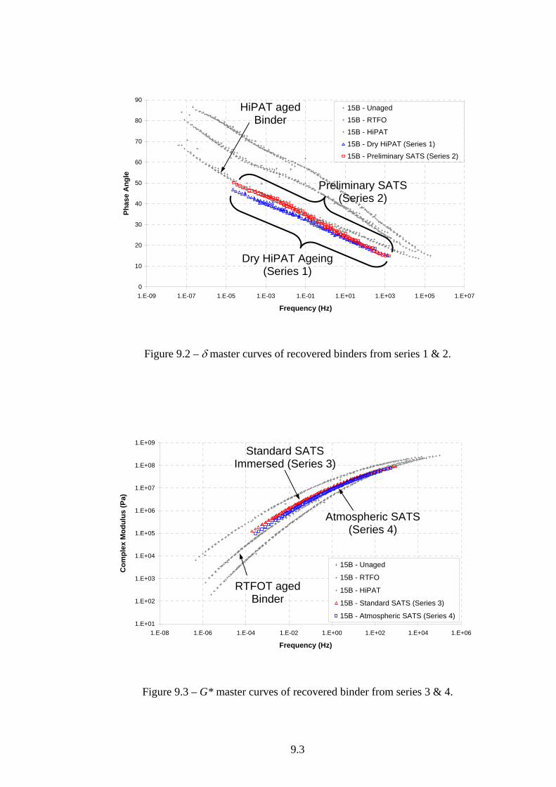
9.3

Figure 9.2 – δ master curves of recovered binders from series 1 & 2.

Figure 9.3 – G* master curves of recovered binder from series 3 & 4.

0

10

20

30

40

50

60

70

80

90

1.E-09 1.E-07 1.E-05 1.E-03 1.E-01 1.E+01 1.E+03 1.E+05 1.E+07

Frequency (Hz)

Phas

e A

ngle

15B - Unaged15B - RTFO15B - HiPAT15B - Dry HiPAT (Series 1)15B - Preliminary SATS (Series 2)

Preliminary SATS (Series 2)

HiPAT aged Binder

Dry HiPAT Ageing (Series 1)

1.E+01

1.E+02

1.E+03

1.E+04

1.E+05

1.E+06

1.E+07

1.E+08

1.E+09

1.E-08 1.E-06 1.E-04 1.E-02 1.E+00 1.E+02 1.E+04 1.E+06

Frequency (Hz)

Com

plex

Mod

ulus

(Pa)

15B - Unaged

15B - RTFO

15B - HiPAT

15B - Standard SATS (Series 3)

15B - Atmospheric SATS (Series 4)

Standard SATS Immersed (Series 3)

RTFOT aged Binder

Atmospheric SATS (Series 4)

9.4

Figure 9.4 – δ master curves of recovered binder from series 3 & 4.

Figures 9.1 and 9.2 clearly show that the binders recovered after the preliminary

SATS protocol (Series 2, initial vacuum saturation only, no added water) and the

Dry HiPAT ageing process (Series 1) typically have very similar rheological

characteristics to those of the HiPAT aged binder indicating a similar amount of

ageing.

Figures 9.3 and 9.4 present the recovered binder DSR results from Atmospheric

SATS (no added pressure) and immersed specimens from the standard SATS (2.1

MPa, 85oC, 65 hrs). Both sets of results typically showed considerably less ageing

than the Series 1 and 2 (i.e. more comparable to RTFOT aged binder). It is

interesting to note that the recovered binder from fully immersed specimens showed

considerably less ageing than those from the Series 1 and 2 although the test

conditions (pressure, temperature and test duration) are identical. It is thought that

the specimens were ‘insulated’ from air by the surrounding water resulting in much

less air contact than those from the specimens above water level.

10

20

30

40

50

60

70

80

90

1.E-09 1.E-07 1.E-05 1.E-03 1.E-01 1.E+01 1.E+03 1.E+05 1.E+07

Frequency (Hz)

Phas

e A

ngle

15B - Unaged

15B - RTFO

15B - HiPAT

15B - Standard SATS (Series 3)

15B - Atmospheric SATS (Series 4)

Standard SATS Immersed (Series 3)

RTFOT aged Binder

Atmospheric SATS (Series 4)

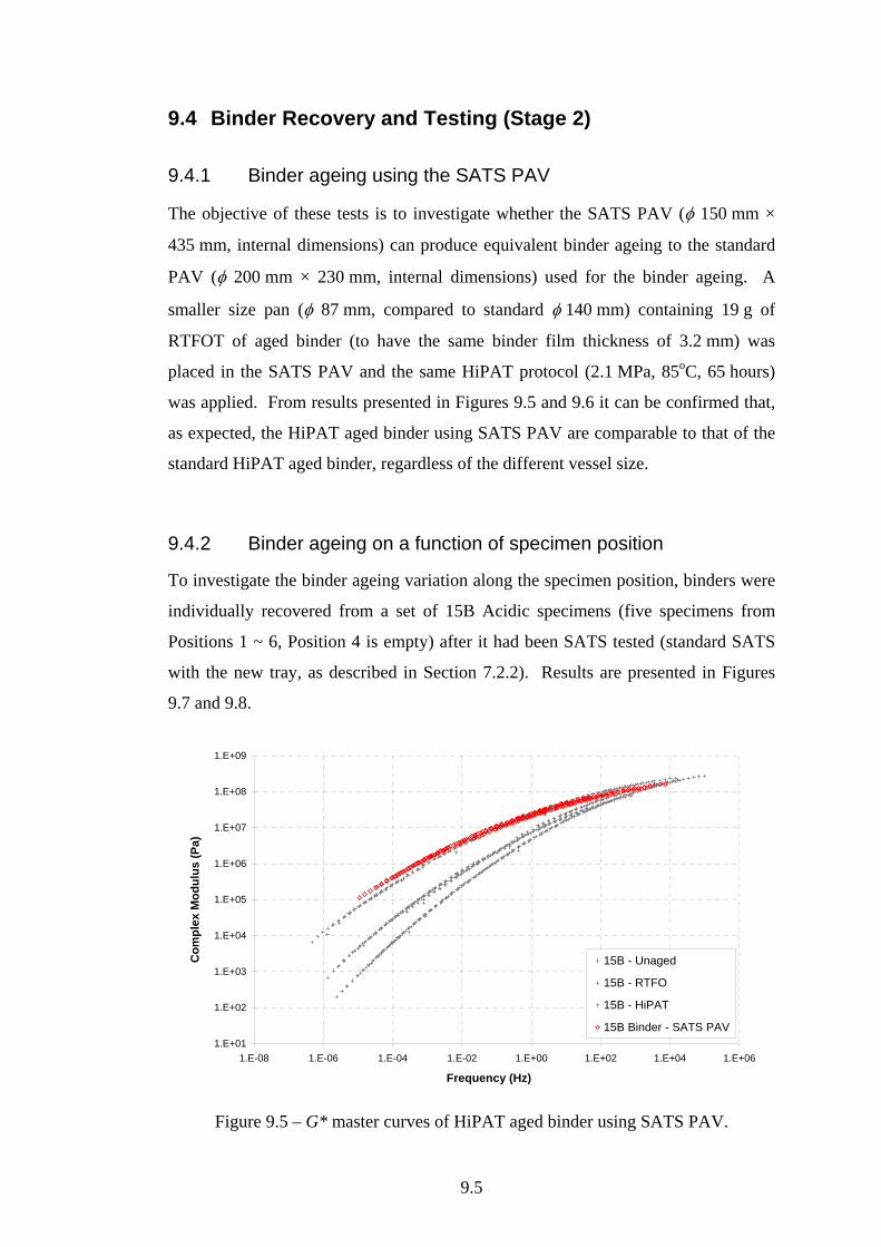
9.5

9.4 Binder Recovery and Testing (Stage 2)

9.4.1 Binder ageing using the SATS PAV

The objective of these tests is to investigate whether the SATS PAV (φ 150 mm ×

435 mm, internal dimensions) can produce equivalent binder ageing to the standard

PAV (φ 200 mm × 230 mm, internal dimensions) used for the binder ageing. A

smaller size pan (φ 87 mm, compared to standard φ 140 mm) containing 19 g of

RTFOT of aged binder (to have the same binder film thickness of 3.2 mm) was

placed in the SATS PAV and the same HiPAT protocol (2.1 MPa, 85oC, 65 hours)

was applied. From results presented in Figures 9.5 and 9.6 it can be confirmed that,

as expected, the HiPAT aged binder using SATS PAV are comparable to that of the

standard HiPAT aged binder, regardless of the different vessel size.

9.4.2 Binder ageing on a function of specimen position

To investigate the binder ageing variation along the specimen position, binders were

individually recovered from a set of 15B Acidic specimens (five specimens from

Positions 1 ~ 6, Position 4 is empty) after it had been SATS tested (standard SATS

with the new tray, as described in Section 7.2.2). Results are presented in Figures

9.7 and 9.8.

1.E+01

1.E+02

1.E+03

1.E+04

1.E+05

1.E+06

1.E+07

1.E+08

1.E+09

1.E-08 1.E-06 1.E-04 1.E-02 1.E+00 1.E+02 1.E+04 1.E+06

Frequency (Hz)

Com

plex

Mod

ulus

(Pa)

15B - Unaged

15B - RTFO

15B - HiPAT

15B Binder - SATS PAV

Figure 9.5 – G* master curves of HiPAT aged binder using SATS PAV.

9.6

0

10

20

30

40

50

60

70

80

90

1.E-10 1.E-08 1.E-06 1.E-04 1.E-02 1.E+00 1.E+02 1.E+04 1.E+06

Frequency (Hz)

Phas

e A

ngle

15B - Unaged

15B - RTFO

15B - HiPAT

15B Binder - SATS PAV

Figure 9.6 – δ master curves of HiPAT aged binder using SATS PAV.

Figure 9.7 – G* master curves of recovered binders from 15B Acidic SATS.

1.E+01

1.E+02

1.E+03

1.E+04

1.E+05

1.E+06

1.E+07

1.E+08

1.E+09

1.E-08 1.E-06 1.E-04 1.E-02 1.E+00 1.E+02 1.E+04 1.E+06

Frequency (Hz)

Com

plex

Mod

ulus

(Pa)

15B - Unaged

15B - RTFO

15B - HiPAT

15B Acidic - P1

15B Acidic - P2

15B Acidic - P3

15B Acidic - P4

15B Acidic - P6HiPAT aged binder

Position 2

Position 3

Position 4

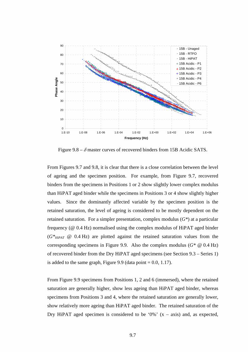
9.7

0

10

20

30

40

50

60

70

80

90

1.E-10 1.E-08 1.E-06 1.E-04 1.E-02 1.E+00 1.E+02 1.E+04 1.E+06

Frequency (Hz)

Phas

e A

ngle

15B - Unaged15B - RTFO15B - HiPAT15B Acidic - P115B Acidic - P215B Acidic - P315B Acidic - P415B Acidic - P6

Figure 9.8 – δ master curves of recovered binders from 15B Acidic SATS.

From Figures 9.7 and 9.8, it is clear that there is a close correlation between the level

of ageing and the specimen position. For example, from Figure 9.7, recovered

binders from the specimens in Positions 1 or 2 show slightly lower complex modulus

than HiPAT aged binder while the specimens in Positions 3 or 4 show slightly higher

values. Since the dominantly affected variable by the specimen position is the

retained saturation, the level of ageing is considered to be mostly dependent on the

retained saturation. For a simpler presentation, complex modulus (G*) at a particular

frequency (@ 0.4 Hz) normalised using the complex modulus of HiPAT aged binder

(G*HiPAT @ 0.4 Hz) are plotted against the retained saturation values from the

corresponding specimens in Figure 9.9. Also the complex modulus (G* @ 0.4 Hz)

of recovered binder from the Dry HiPAT aged specimens (see Section 9.3 – Series 1)

is added to the same graph, Figure 9.9 (data point = 0.0, 1.17).

From Figure 9.9 specimens from Positions 1, 2 and 6 (immersed), where the retained

saturation are generally higher, show less ageing than HiPAT aged binder, whereas

specimens from Positions 3 and 4, where the retained saturation are generally lower,

show relatively more ageing than HiPAT aged binder. The retained saturation of the

Dry HiPAT aged specimen is considered to be ‘0%’ (x – axis) and, as expected,

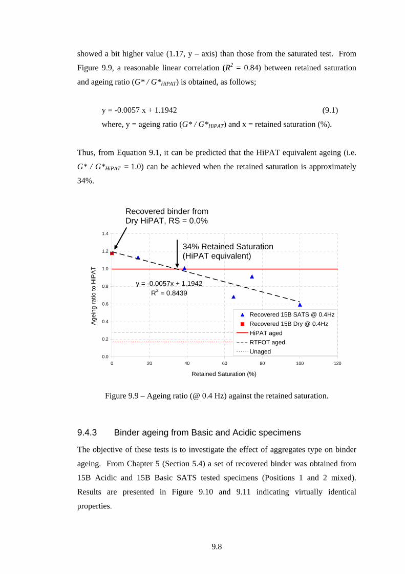
9.8

showed a bit higher value (1.17, y – axis) than those from the saturated test. From

Figure 9.9, a reasonable linear correlation (R2 = 0.84) between retained saturation

and ageing ratio (G* / G*HiPAT) is obtained, as follows;

y = -0.0057 x + 1.1942 (9.1)

where, y = ageing ratio (G* / G*HiPAT) and x = retained saturation (%).

Thus, from Equation 9.1, it can be predicted that the HiPAT equivalent ageing (i.e.

G* / G*HiPAT = 1.0) can be achieved when the retained saturation is approximately

34%.

Figure 9.9 – Ageing ratio (@ 0.4 Hz) against the retained saturation.

9.4.3 Binder ageing from Basic and Acidic specimens

The objective of these tests is to investigate the effect of aggregates type on binder

ageing. From Chapter 5 (Section 5.4) a set of recovered binder was obtained from

15B Acidic and 15B Basic SATS tested specimens (Positions 1 and 2 mixed).

Results are presented in Figure 9.10 and 9.11 indicating virtually identical

properties.

y = -0.0057x + 1.1942R2 = 0.8439

0.0

0.2

0.4

0.6

0.8

1.0

1.2

1.4

0 20 40 60 80 100 120

Retained Saturation (%)

Age

ing

ratio

to H

iPA

T

Recovered 15B SATS @ 0.4HzRecovered 15B Dry @ 0.4HzHiPAT agedRTFOT agedUnaged

34% Retained Saturation (HiPAT equivalent)

Recovered binder from Dry HiPAT, RS = 0.0%

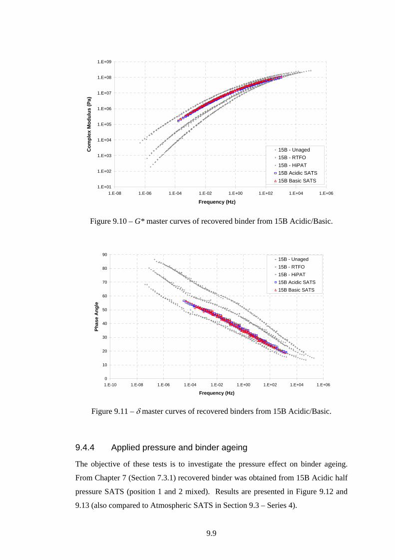
9.9

1.E+01

1.E+02

1.E+03

1.E+04

1.E+05

1.E+06

1.E+07

1.E+08

1.E+09

1.E-08 1.E-06 1.E-04 1.E-02 1.E+00 1.E+02 1.E+04 1.E+06

Frequency (Hz)

Com

plex

Mod

ulus

(Pa)

15B - Unaged15B - RTFO15B - HiPAT15B Acidic SATS15B Basic SATS

Figure 9.10 – G* master curves of recovered binder from 15B Acidic/Basic.

0

10

20

30

40

50

60

70

80

90

1.E-10 1.E-08 1.E-06 1.E-04 1.E-02 1.E+00 1.E+02 1.E+04 1.E+06

Frequency (Hz)

Phas

e A

ngle

15B - Unaged15B - RTFO15B - HiPAT15B Acidic SATS15B Basic SATS

Figure 9.11 – δ master curves of recovered binders from 15B Acidic/Basic.

9.4.4 Applied pressure and binder ageing

The objective of these tests is to investigate the pressure effect on binder ageing.

From Chapter 7 (Section 7.3.1) recovered binder was obtained from 15B Acidic half

pressure SATS (position 1 and 2 mixed). Results are presented in Figure 9.12 and

9.13 (also compared to Atmospheric SATS in Section 9.3 – Series 4).

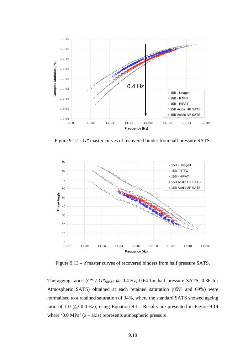
9.10

Figure 9.12 – G* master curves of recovered binder from half pressure SATS.

0

10

20

30

40

50

60

70

80

90

1.E-10 1.E-08 1.E-06 1.E-04 1.E-02 1.E+00 1.E+02 1.E+04 1.E+06

Frequency (Hz)

Phas

e A

ngle

15B - Unaged

15B - RTFO

15B - HiPAT

15B Acidic HP SATS

15B Acidic AP SATS

Figure 9.13 – δ master curves of recovered binders from half pressure SATS.

The ageing ratios (G* / G*HiPAT @ 0.4 Hz, 0.64 for half pressure SATS, 0.36 for

Atmospheric SATS) obtained at each retained saturation (85% and 69%) were

normalised to a retained saturation of 34%, where the standard SATS showed ageing

ratio of 1.0 (@ 0.4 Hz), using Equation 9.1. Results are presented in Figure 9.14

where ‘0.0 MPa’ (x – axis) represents atmospheric pressure.

1.E+01

1.E+02

1.E+03

1.E+04

1.E+05

1.E+06

1.E+07

1.E+08

1.E+09

1.E-08 1.E-06 1.E-04 1.E-02 1.E+00 1.E+02 1.E+04 1.E+06

Frequency (Hz)

Com

plex

Mod

ulus

(Pa)

15B - Unaged

15B - RTFO

15B - HiPAT

15B Acidic HP SATS

15B Acidic AP SATS

0.4 Hz

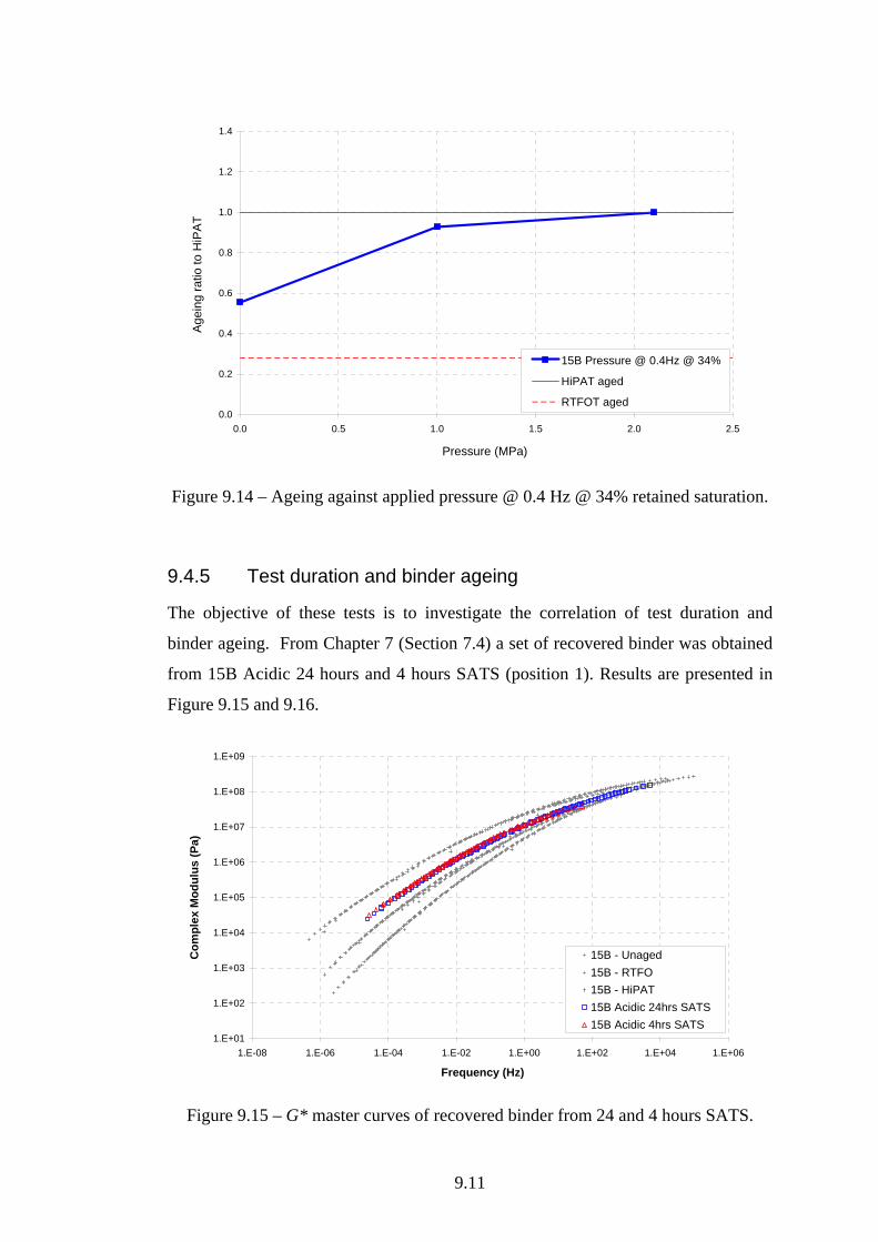
9.11

0.0

0.2

0.4

0.6

0.8

1.0

1.2

1.4

0.0 0.5 1.0 1.5 2.0 2.5

Pressure (MPa)

Age

ing

ratio

to H

iPA

T

15B Pressure @ 0.4Hz @ 34%

HiPAT aged

RTFOT aged

Figure 9.14 – Ageing against applied pressure @ 0.4 Hz @ 34% retained saturation.

9.4.5 Test duration and binder ageing

The objective of these tests is to investigate the correlation of test duration and

binder ageing. From Chapter 7 (Section 7.4) a set of recovered binder was obtained

from 15B Acidic 24 hours and 4 hours SATS (position 1). Results are presented in

Figure 9.15 and 9.16.

1.E+01

1.E+02

1.E+03

1.E+04

1.E+05

1.E+06

1.E+07

1.E+08

1.E+09

1.E-08 1.E-06 1.E-04 1.E-02 1.E+00 1.E+02 1.E+04 1.E+06

Frequency (Hz)

Com

plex

Mod

ulus

(Pa)

15B - Unaged15B - RTFO15B - HiPAT15B Acidic 24hrs SATS15B Acidic 4hrs SATS

Figure 9.15 – G* master curves of recovered binder from 24 and 4 hours SATS.

9.12

0

10

20

30

40

50

60

70

80

90

1.E-10 1.E-08 1.E-06 1.E-04 1.E-02 1.E+00 1.E+02 1.E+04 1.E+06

Frequency (Hz)

Phas

e A

ngle

15B - Unaged15B - RTFO15B - HiPAT15B Acidic 24hrs SATS15B Acidic 4hrs SATS

Figure 9.16 – δ master curves of recovered binders from 24 and 4 hours SATS.

The normalised ageing ratio (to a retained saturation of 34%) against the test

duration, as described in the previous section, are presented in Figure 9.17.

0.0

0.2

0.4

0.6

0.8

1.0

1.2

1.4

0 10 20 30 40 50 60 70

Duration (hrs)

Age

ing

ratio

to H

iPA

T

15B Duration @ 0.4Hz @ 34%

HiPAT aged

RTFOT aged

Figure 9.17 – Ageing against test duration @ 0.4 Hz @ 34% retained saturation.

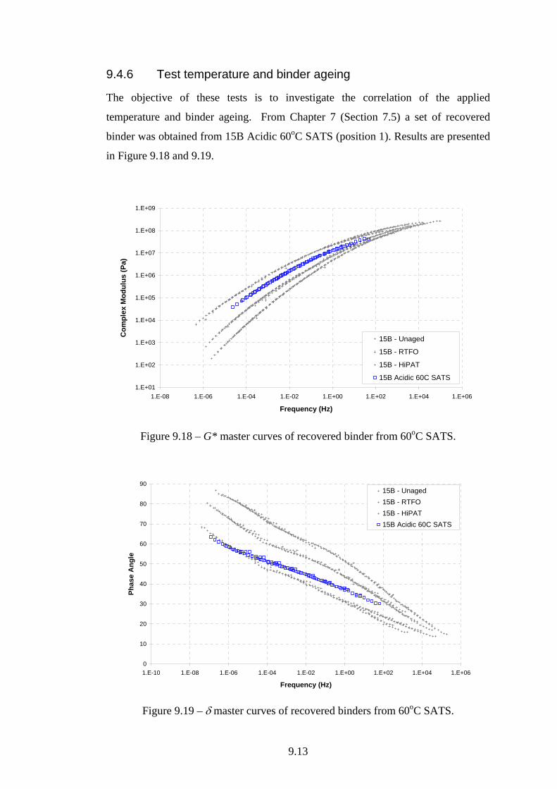
9.13

9.4.6 Test temperature and binder ageing

The objective of these tests is to investigate the correlation of the applied

temperature and binder ageing. From Chapter 7 (Section 7.5) a set of recovered

binder was obtained from 15B Acidic 60oC SATS (position 1). Results are presented

in Figure 9.18 and 9.19.

1.E+01

1.E+02

1.E+03

1.E+04

1.E+05

1.E+06

1.E+07

1.E+08

1.E+09

1.E-08 1.E-06 1.E-04 1.E-02 1.E+00 1.E+02 1.E+04 1.E+06

Frequency (Hz)

Com

plex

Mod

ulus

(Pa)

15B - Unaged

15B - RTFO

15B - HiPAT

15B Acidic 60C SATS

Figure 9.18 – G* master curves of recovered binder from 60oC SATS.

0

10

20

30

40

50

60

70

80

90

1.E-10 1.E-08 1.E-06 1.E-04 1.E-02 1.E+00 1.E+02 1.E+04 1.E+06

Frequency (Hz)

Phas

e A

ngle

15B - Unaged15B - RTFO15B - HiPAT15B Acidic 60C SATS

Figure 9.19 – δ master curves of recovered binders from 60oC SATS.

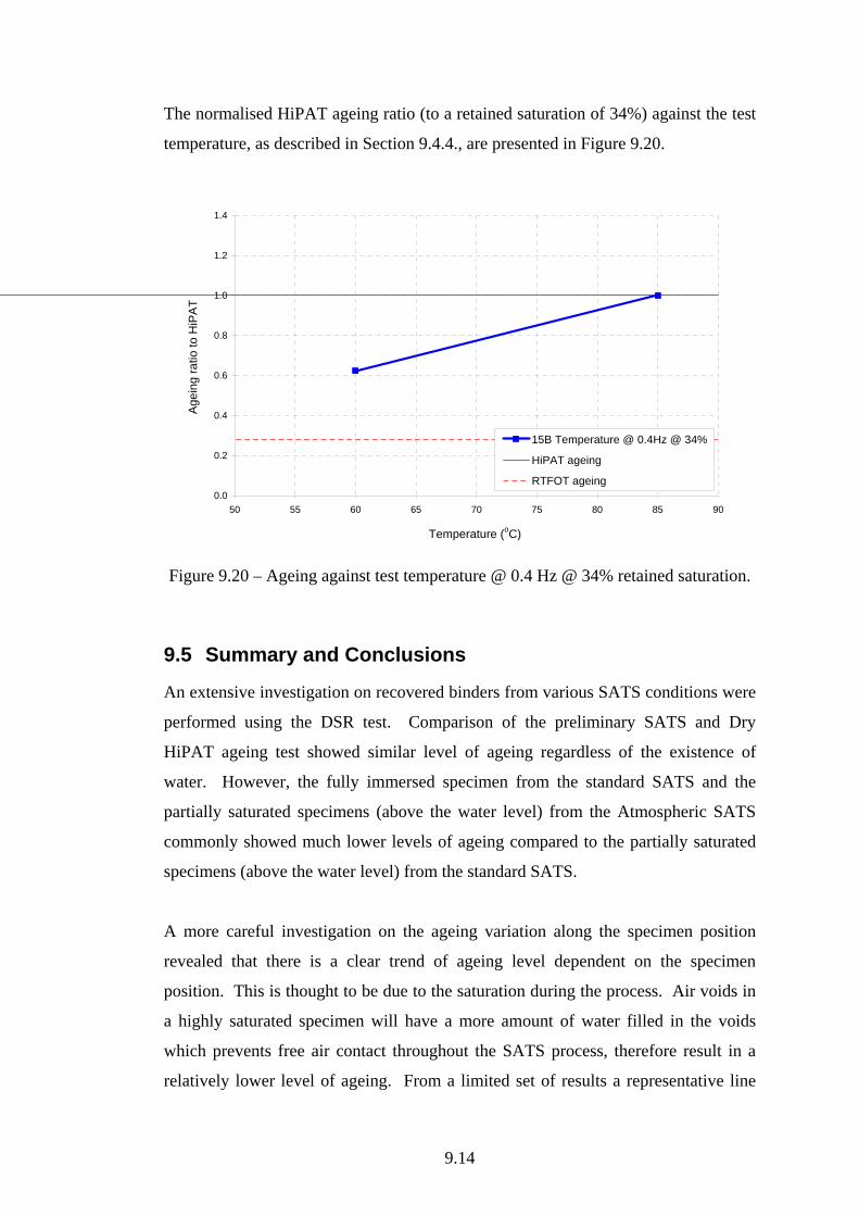
9.14

The normalised HiPAT ageing ratio (to a retained saturation of 34%) against the test

temperature, as described in Section 9.4.4., are presented in Figure 9.20.

0.0

0.2

0.4

0.6

0.8

1.0

1.2

1.4

50 55 60 65 70 75 80 85 90

Temperature (oC)

Age

ing

ratio

to H

iPA

T

15B Temperature @ 0.4Hz @ 34%

HiPAT ageing

RTFOT ageing

Figure 9.20 – Ageing against test temperature @ 0.4 Hz @ 34% retained saturation.

9.5 Summary and Conclusions

An extensive investigation on recovered binders from various SATS conditions were

performed using the DSR test. Comparison of the preliminary SATS and Dry

HiPAT ageing test showed similar level of ageing regardless of the existence of

water. However, the fully immersed specimen from the standard SATS and the

partially saturated specimens (above the water level) from the Atmospheric SATS

commonly showed much lower levels of ageing compared to the partially saturated

specimens (above the water level) from the standard SATS.

A more careful investigation on the ageing variation along the specimen position

revealed that there is a clear trend of ageing level dependent on the specimen

position. This is thought to be due to the saturation during the process. Air voids in

a highly saturated specimen will have a more amount of water filled in the voids

which prevents free air contact throughout the SATS process, therefore result in a

relatively lower level of ageing. From a limited set of results a representative line

9.15

was fitted and a retained saturation of 34% has been found to be the HiPAT

equivalent ageing condition (i.e. G* / G*HiPAT = 1.0) for the 15B Acidic control

mixture from the standard SATS protocol.

A series of recovered binder from various SATS conditions (lower pressures, shorter

test durations and lower temperatures) revealed that, to achieve a HiPAT equivalent

binder ageing from the SATS protocol within the same testing duration (65 hours),

the pressure and temperature conditions used in the standard SATS (2.1 MPa and

85oC) are necessary.

10.1

Chapter 10. Data Interpretation

10.1 Retained Saturation

From a large number of SATS data observed in the previous chapters, it was noted

that some results from the SATS test showed retained saturations higher than 100%.

Saturation over 100% is not a realistic value, indicating a certain volumetric change

took place during the test. For an example, a 15B Acidic result from Atmospheric

SATS test performed in Section 7.3.2 (data not presented in Figure 7.6) showed a

retained saturation value of 141% (from the immersed specimen) with clearly visible

swelling (near disintegration stage, retained stiffness of 0.1). As the apparent

volume of the specimen was expanded, the internal voids content was also

supposedly increased. A series of SATS tested specimens were selected and the air voids were measured

again (referred to as ‘retained AV’) using the identical method to that described in

Section 5.2.2. Table 10.1 (Column 5) shows the retained AV of 15B Acidic

specimens which have been tested using the standard SATS, half pressure SATS or

Atmospheric SATS protocol (see Section 7.3). The retained AV data of 15B Basic

specimens are also presented in Table 10.2 (Column 5). Tables 10.1 and 10.2 also

show the retained saturations calculated using the ‘initial AV’ (referred to as

‘Satnominal’, in Column 6) and the retained saturation calculated using the ‘retained

AV’ (referred to as ‘Satactual’, in Column 7). The reason of selecting specimens from

SATS tests using different pressures was to observe whether the applied pressure

particularly contributed to change the volumetric properties.

From Table 10.1 (15B Acidic series), it is noted that the retained saturations

(Satnominal) over 100% are commonly associated with very low retained stiffnesses

(≤ 0.1), regardless of the magnitude of applied pressure. This low retained stiffness

clearly indicates that the specimens are in a near disintegrating state with a much

increased internal voids due to the creation of cracks or adhesion failure between

binder and aggregate. It can be found from Table 10.2 that the 15B Basic specimen

from Atmospheric SATS displays virtually unchanged air voids resulting in

10.2

unchanged retained saturations (Nominal/Actual ratio ≈ 1.0). 15B Basic specimens

from the pressurised SATS protocols commonly show increased Nominal/Actual

ratio (1.2 ~ 1.4) due to a pressure related damage (see Section 7.3.2 for a more

discussion). This fact generally agrees with the finding from Chapters 7 and 8,

where 15B Acidic mixtures are considered to be pressure insusceptible and 15B

Basic mixtures to be pressure susceptible. However, in general, it should be noted

that the bigger volumetric change (i.e. higher Nominal/Actual ratio) is associated

with the lower retained stiffness values (i.e. more damage), regardless of the applied

pressure or material types.

Table 10.1 – Air voids and retained saturation chart of 15B Acidic specimens.

15B Acidic control Retained

stiffness Initial AV

Retained AV

Satnominal (%)

Satactual (%)

Nominal /Actual

Standard 1 0.73 8.02 9.57 5.5 4.5 1.21 SATS 2 0.16 9.24 12.77 79.7 55.5 1.44

3 0.01 7.83 15.53 142.1 65.6 2.17

Half P 1 0.05 7.89 11.72 96.8 62.5 1.55 SATS 2 0.05 9.19 11.94 68.5 51.2 1.34

3 0.13 7.36 10.59 72.5 48.6 1.49 4 0.26 7.31 9.72 39.5 31.2 1.27

Atmospheric 1 0.27 9.51 10.57 81.6 74.7 1.09 SATS 2 0.25 7.98 9.60 92.4 77.9 1.19

3 0.10 7.93 11.73 140.8 93.0 1.51

Table 10.2 – Air voids and retained saturation chart of 15B Basic specimens.

15B Basic control Retained

stiffness Initial AV

Retained AV

Satnominal (%)

Satactual (%)

Nominal /Actual

Standard SATS 1 0.77 7.43 10.13 27.0 19.2 1.40

Half P 1 0.80 9.68 11.28 50.6 42.6 1.19 SATS 2 0.70 7.30 9.24 53.7 41.5 1.29

3 0.77 7.32 9.18 84.8 66.3 1.28

Atmospheric 1 0.92 8.71 8.88 50.7 49.7 1.02 SATS 2 0.93 8.50 8.52 56.1 55.9 1.00

3 0.93 8.91 8.95 42.6 42.4 1.00 4 0.97 10.4 10.13 32.0 31.7 1.01 5 0.97 9.61 9.93 61.3 59.1 1.04

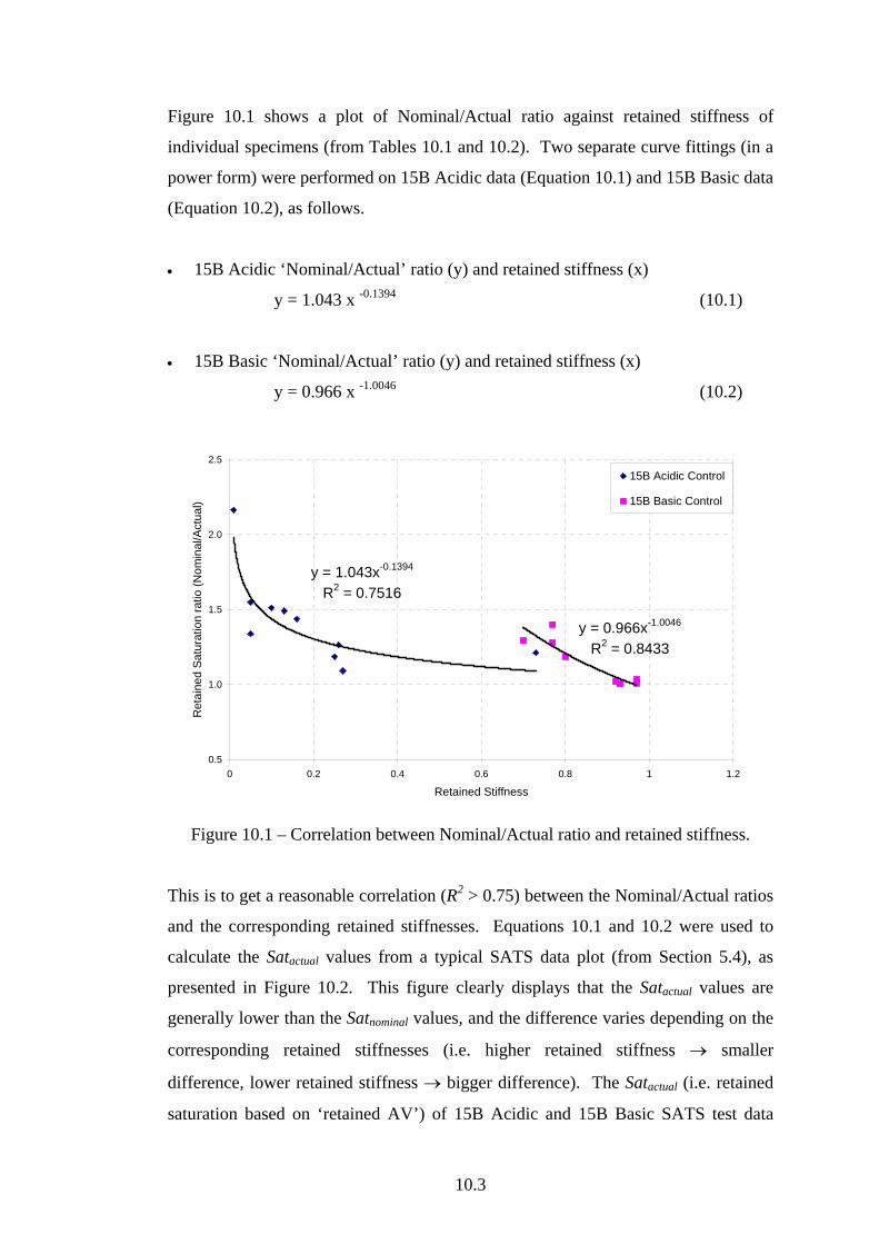
10.3

Figure 10.1 shows a plot of Nominal/Actual ratio against retained stiffness of

individual specimens (from Tables 10.1 and 10.2). Two separate curve fittings (in a

power form) were performed on 15B Acidic data (Equation 10.1) and 15B Basic data

(Equation 10.2), as follows.

• 15B Acidic ‘Nominal/Actual’ ratio (y) and retained stiffness (x)

y = 1.043 x -0.1394 (10.1)

• 15B Basic ‘Nominal/Actual’ ratio (y) and retained stiffness (x)

y = 0.966 x -1.0046 (10.2)

y = 1.043x-0.1394

R2 = 0.7516

y = 0.966x-1.0046

R2 = 0.8433

0.5

1.0

1.5

2.0

2.5

0 0.2 0.4 0.6 0.8 1 1.2

Retained Stiffness

Ret

aine

d S

atur

atio

n ra

tio (N

omin

al/A

ctua

l)

15B Acidic Control

15B Basic Control

Figure 10.1 – Correlation between Nominal/Actual ratio and retained stiffness.

This is to get a reasonable correlation (R2 > 0.75) between the Nominal/Actual ratios

and the corresponding retained stiffnesses. Equations 10.1 and 10.2 were used to

calculate the Satactual values from a typical SATS data plot (from Section 5.4), as

presented in Figure 10.2. This figure clearly displays that the Satactual values are

generally lower than the Satnominal values, and the difference varies depending on the

corresponding retained stiffnesses (i.e. higher retained stiffness → smaller

difference, lower retained stiffness → bigger difference). The Satactual (i.e. retained

saturation based on ‘retained AV’) of 15B Acidic and 15B Basic SATS test data

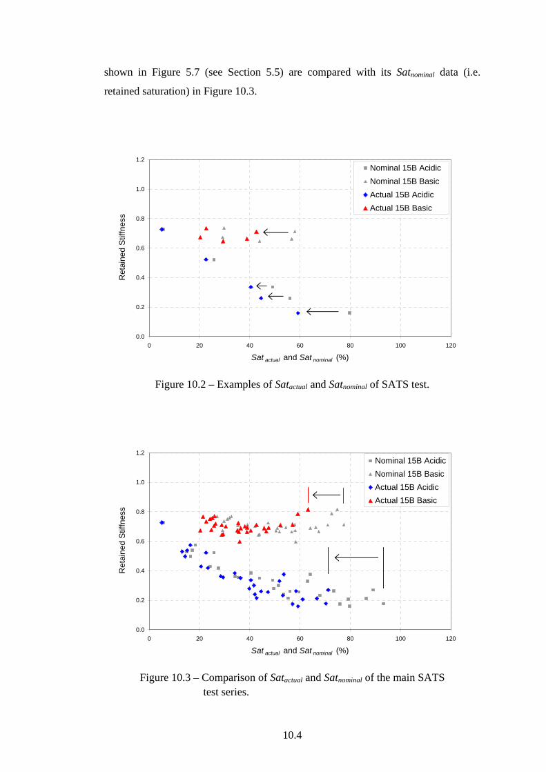
10.4

shown in Figure 5.7 (see Section 5.5) are compared with its Satnominal data (i.e.

retained saturation) in Figure 10.3.

Figure 10.2 – Examples of Satactual and Satnominal of SATS test.

Figure 10.3 – Comparison of Satactual and Satnominal of the main SATS

test series.

0.0

0.2

0.4

0.6

0.8

1.0

1.2

0 20 40 60 80 100 120

Sat actual and Sat nominal (%)

Ret

aine

d S

tiffn

ess

Nominal 15B AcidicNominal 15B BasicActual 15B AcidicActual 15B Basic

0.0

0.2

0.4

0.6

0.8

1.0

1.2

0 20 40 60 80 100 120

Sat actual and Sat nominal (%)

Ret

aine

d S

tiffn

ess

Nominal 15B AcidicNominal 15B BasicActual 15B AcidicActual 15B Basic

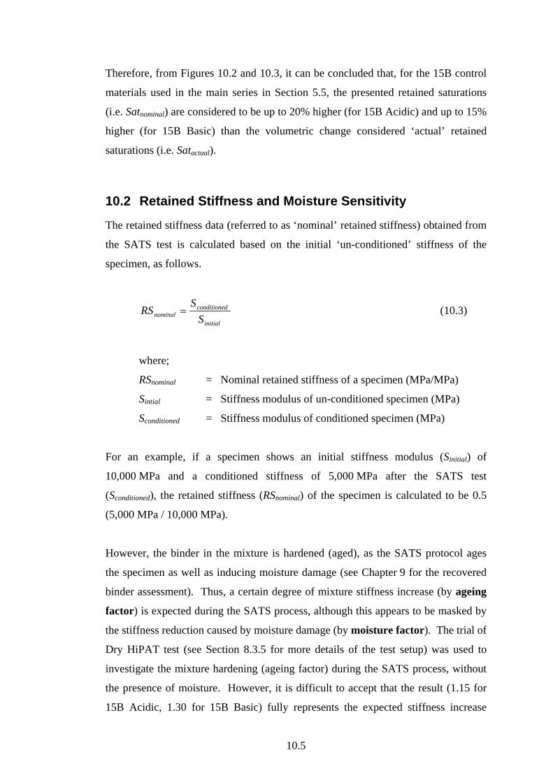
10.5

Therefore, from Figures 10.2 and 10.3, it can be concluded that, for the 15B control

materials used in the main series in Section 5.5, the presented retained saturations

(i.e. Satnominal) are considered to be up to 20% higher (for 15B Acidic) and up to 15%

higher (for 15B Basic) than the volumetric change considered ‘actual’ retained

saturations (i.e. Satactual).

10.2 Retained Stiffness and Moisture Sensitivity

The retained stiffness data (referred to as ‘nominal’ retained stiffness) obtained from

the SATS test is calculated based on the initial ‘un-conditioned’ stiffness of the

specimen, as follows.

initial

dconditionenominal S

SRS = (10.3)

where;

RSnominal = Nominal retained stiffness of a specimen (MPa/MPa)

Sintial = Stiffness modulus of un-conditioned specimen (MPa)

Sconditioned = Stiffness modulus of conditioned specimen (MPa)

For an example, if a specimen shows an initial stiffness modulus (Sinitial) of

10,000 MPa and a conditioned stiffness of 5,000 MPa after the SATS test

(Sconditioned), the retained stiffness (RSnominal) of the specimen is calculated to be 0.5

(5,000 MPa / 10,000 MPa).

However, the binder in the mixture is hardened (aged), as the SATS protocol ages

the specimen as well as inducing moisture damage (see Chapter 9 for the recovered

binder assessment). Thus, a certain degree of mixture stiffness increase (by ageing

factor) is expected during the SATS process, although this appears to be masked by

the stiffness reduction caused by moisture damage (by moisture factor). The trial of

Dry HiPAT test (see Section 8.3.5 for more details of the test setup) was used to

investigate the mixture hardening (ageing factor) during the SATS process, without

the presence of moisture. However, it is difficult to accept that the result (1.15 for

15B Acidic, 1.30 for 15B Basic) fully represents the expected stiffness increase

10.6

entirely due to the ‘ageing factor’ of SATS protocol, as a certain degree of pressure

damage (by pressure factor) is presumed to be included in the results (see Section

7.6 for more discussions on the pressure damage).

Therefore the SATS conditioned stiffness modulus (Sconditioned) of a specimen can be

expressed as follows.

moisturepressureageinginitialdconditione fffSS ×××= (10.4)

where;

Sintial = Stiffness modulus of unconditioned specimen (MPa)

Sconditioned = Stiffness modulus of conditioned specimen (MPa)

fageing = Ageing factor (age hardening of mixture)

fpressure = Pressure factor (pressure damage)

fmoisture = Moisture factor (moisture sensitivity)

Consequently, once the ageing factor (fageing) and pressure factor (fpressure) are

identified, the ‘true’ moisture sensitivity (fmoisture) of a SATS conditioned specimen

can be obtained as follows.

pressureageing

nominal

pressureageinginitial

dconditionemoisture ff

RSffS

Sf

×=

××= (10.5)

10.3 Ageing Hardening (fageing)

The binder in the mixture from the SATS test is expected to be aged equivalent to

the HiPAT binder ageing level (in a specific retained saturation of 34%, see Section

9.4.2). It is easily predicted that, if the binder in the mixture hardens (binder

stiffness increases), the mixture stiffness will also increase. However, the correlation

between the binder stiffness increase and the resultant mixture stiffness increase does

not seem to be linear. For an example, the DSR test performed on the HiPAT aged

15B binder shows approximately 3.5 times higher complex modulus (G*) than that

of the RTFOT aged 15B binder (see Appendix C). If this ratio is directly applied on

10.7

the mixture stiffness, then the stiffness of 15B Acidic or Basic specimens (due to

binder ageing) would increase up to 35,000 MPa (3.5 × unconditioned mixture

stiffness (Sinitial) of 10,000 MPa), which is an unrealistically high value for the

bituminous materials (the binder of ‘unconditioned’ specimens was defined to have

same complex modulus to that of RTFOT aged binder).

To find the correlation between binder stiffness change and resultant mixture

stiffness change, the Shell BANDS 2.0 software [Shell Bitumen, 1998] has been

used. This programme is based on a binder stiffness prediction nomograph produced

by Van der Poel [1954] and a mixture stiffness prediction nomograph produced by

Bonnaure et al. [1977]. Van der Poel [1954] produced the nomograph (see

Figure 10.4) based on the data from series of stiffness determination tests conducted

on forty bitumen binders at many temperatures and frequencies, using both creep and

dynamic tests. This nomograph is to predict the stiffness modulus of a bitumen for

any conditions of temperature and loading time, using only Penetration and

Softening point data, within a practically acceptable range (factor of 2). Bonnaure et

al. [1977] conducted series of dynamic tests (2 point and 3 point bending tests) on

twelve bituminous mixtures of vastly different composition but representative of

mixtures used in a number of countries. As a result, they produced the nomograph

shown in Figure 10.5 for predicting the stiffness modulus of a bituminous material.

The input required for this nomograph are a) stiffness modulus of bitumen (Pa)

obtained from the Van der Poel nomograph, b) volume of bitumen (Vb, %) and c)

volume of mineral aggregates (Va, %). It should be noted that the stiffness modulus

of bitumen was from the ‘recovered’ binder from the tested mixtures, not from the

initial ‘fresh’ binder to make the mixtures.

10.3.1 Binder stiffness prediction (Van der Poel Nomograph)

The Penetration and Softening point data of unaged, RTFOT aged or HiPAT aged

15B binders (see Table 10.3, data also presented in Appendix C) are used to predict

binder stiffness using the BANDS software. As observed in Table 10.3, the

measured ‘tensile’ stiffnesses (G* × 3) from DSR test (under 2 Hz sinusoidal loading

and 20oC test temperature) are considerably lower (around 60%) than the BANDS

predicted binder stiffnesses (using Penetration and Softening point test data, for a

10.8

Figure 10.4 – Nomograph for determining stiffness modulus of bitumens

[Van der Poel, 1954].

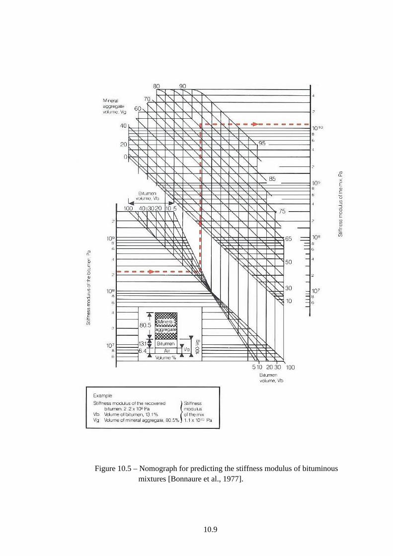
10.9

Figure 10.5 – Nomograph for predicting the stiffness modulus of bituminous mixtures [Bonnaure et al., 1977].

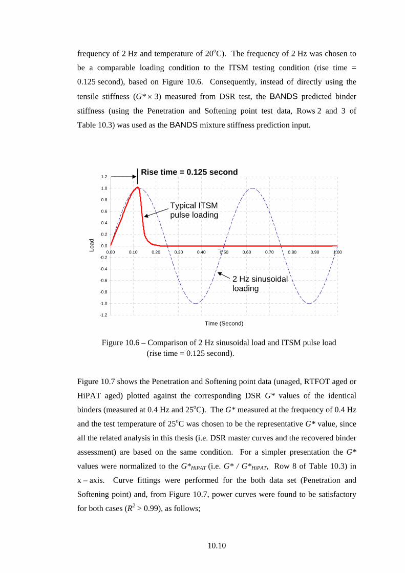
10.10

frequency of 2 Hz and temperature of 20oC). The frequency of 2 Hz was chosen to

be a comparable loading condition to the ITSM testing condition (rise time =

0.125 second), based on Figure 10.6. Consequently, instead of directly using the

tensile stiffness (G* × 3) measured from DSR test, the BANDS predicted binder

stiffness (using the Penetration and Softening point test data, Rows 2 and 3 of

Table 10.3) was used as the BANDS mixture stiffness prediction input.

Figure 10.6 – Comparison of 2 Hz sinusoidal load and ITSM pulse load

(rise time = 0.125 second).

Figure 10.7 shows the Penetration and Softening point data (unaged, RTFOT aged or

HiPAT aged) plotted against the corresponding DSR G* values of the identical

binders (measured at 0.4 Hz and 25oC). The G* measured at the frequency of 0.4 Hz

and the test temperature of 25oC was chosen to be the representative G* value, since

all the related analysis in this thesis (i.e. DSR master curves and the recovered binder

assessment) are based on the same condition. For a simpler presentation the G*

values were normalized to the G*HiPAT (i.e. G* / G*HiPAT, Row 8 of Table 10.3) in

x – axis. Curve fittings were performed for the both data set (Penetration and

Softening point) and, from Figure 10.7, power curves were found to be satisfactory

for both cases (R2 > 0.99), as follows;

-1.2

-1.0

-0.8

-0.6

-0.4

-0.2

0.0

0.2

0.4

0.6

0.8

1.0

1.2

0.00 0.10 0.20 0.30 0.40 0.50 0.60 0.70 0.80 0.90 1.00

Time (Second)

Load

```

2 Hz sinusoidal loading

Typical ITSM pulse loading

Rise time = 0.125 second

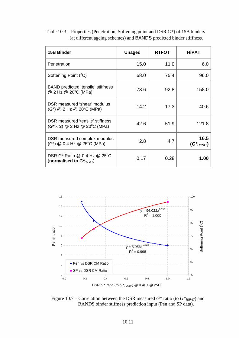
10.11

Table 10.3 – Properties (Penetration, Softening point and DSR G*) of 15B binders (at different ageing schemes) and BANDS predicted binder stiffness.

15B Binder Unaged RTFOT HiPAT

Penetration 15.0 11.0 6.0

Softening Point (oC) 68.0 75.4 96.0

BAND predicted ‘tensile’ stiffness @ 2 Hz @ 20oC (MPa) 73.6 92.8 158.0

DSR measured ‘shear’ modulus (G*) @ 2 Hz @ 20oC (MPa) 14.2 17.3 40.6

DSR measured ‘tensile’ stiffness (G* × 3) @ 2 Hz @ 20oC (MPa) 42.6 51.9 121.8

DSR measured complex modulus (G*) @ 0.4 Hz @ 25oC (MPa) 2.8 4.7 16.5

(G*HiPAT)

DSR G* Ratio @ 0.4 Hz @ 25oC (normalised to G*HiPAT) 0.17 0.28 1.00

y = 96.022x0.193

R2 = 1.000

y = 5.956x-0.507

R2 = 0.998

0

2

4

6

8

10

12

14

16

0.0 0.2 0.4 0.6 0.8 1.0 1.2

DSR G* ratio (to G* HiPAT ) @ 0.4Hz @ 25C

Pen

entra

tion

40

50

60

70

80

90

100

Sof

teni

ng P

oint

(o C)

Pen vs DSR CM Ratio

SP vs DSR CM Ratio

Figure 10.7 – Correlation between the DSR measured G* ratio (to G*HiPAT) and

BANDS binder stiffness prediction input (Pen and SP data).

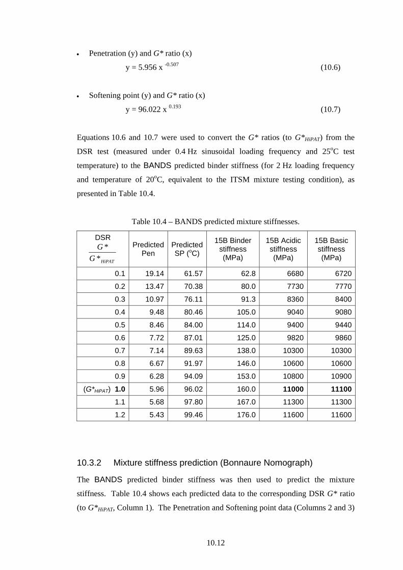
10.12

• Penetration (y) and G* ratio (x)

y = 5.956 x -0.507 (10.6)

• Softening point (y) and G* ratio (x)

y = 96.022 x 0.193 (10.7)

Equations 10.6 and 10.7 were used to convert the G* ratios (to G*HiPAT) from the

DSR test (measured under 0.4 Hz sinusoidal loading frequency and 25oC test

temperature) to the BANDS predicted binder stiffness (for 2 Hz loading frequency

and temperature of 20oC, equivalent to the ITSM mixture testing condition), as

presented in Table 10.4.

Table 10.4 – BANDS predicted mixture stiffnesses.

DSR

HiPATGG*

*

Predicted Pen

PredictedSP (oC)

15B Binder stiffness (MPa)

15B Acidic stiffness (MPa)

15B Basic stiffness (MPa)

0.1 19.14 61.57 62.8 6680 6720

0.2 13.47 70.38 80.0 7730 7770

0.3 10.97 76.11 91.3 8360 8400

0.4 9.48 80.46 105.0 9040 9080

0.5 8.46 84.00 114.0 9400 9440

0.6 7.72 87.01 125.0 9820 9860

0.7 7.14 89.63 138.0 10300 10300

0.8 6.67 91.97 146.0 10600 10600

0.9 6.28 94.09 153.0 10800 10900

(G*HiPAT) 1.0 5.96 96.02 160.0 11000 111001.1 5.68 97.80 167.0 11300 11300

1.2 5.43 99.46 176.0 11600 11600

10.3.2 Mixture stiffness prediction (Bonnaure Nomograph)

The BANDS predicted binder stiffness was then used to predict the mixture

stiffness. Table 10.4 shows each predicted data to the corresponding DSR G* ratio

(to G*HiPAT, Column 1). The Penetration and Softening point data (Columns 2 and 3)

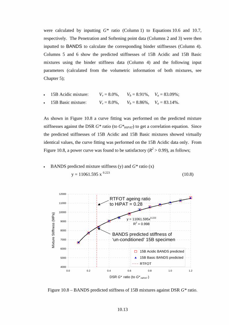
10.13

were calculated by inputting G* ratio (Column 1) to Equations 10.6 and 10.7,

respectively. The Penetration and Softening point data (Columns 2 and 3) were then

inputted to BANDS to calculate the corresponding binder stiffnesses (Column 4).

Columns 5 and 6 show the predicted stiffnesses of 15B Acidic and 15B Basic

mixtures using the binder stiffness data (Column 4) and the following input

parameters (calculated from the volumetric information of both mixtures, see

Chapter 5);

• 15B Acidic mixture: Vv = 8.0%, Vb = 8.91%, Va = 83.09%;

• 15B Basic mixture: Vv = 8.0%, Vb = 8.86%, Va = 83.14%.

As shown in Figure 10.8 a curve fitting was performed on the predicted mixture

stiffnesses against the DSR G* ratio (to G*HiPAT) to get a correlation equation. Since

the predicted stiffnesses of 15B Acidic and 15B Basic mixtures showed virtually

identical values, the curve fitting was performed on the 15B Acidic data only. From

Figure 10.8, a power curve was found to be satisfactory (R2 > 0.99), as follows;

• BANDS predicted mixture stiffness (y) and G* ratio (x)

y = 11061.595 x 0.223 (10.8)

Figure 10.8 – BANDS predicted stiffness of 15B mixtures against DSR G* ratio.

y = 11061.595x0.223

R2 = 0.998

4000

5000

6000

7000

8000

9000

10000

11000

12000

0.0 0.2 0.4 0.6 0.8 1.0 1.2

DSR G* ratio (to G* HiPAT )

Mix

ture

Stif

fnes

s (M

Pa)

15B Acidic BANDS predicted

15B Basic BANDS predicted

RTFOT

BANDS predicted stiffness of ‘un-conditioned’ 15B specimen

RTFOT ageing ratio to HiPAT = 0.28

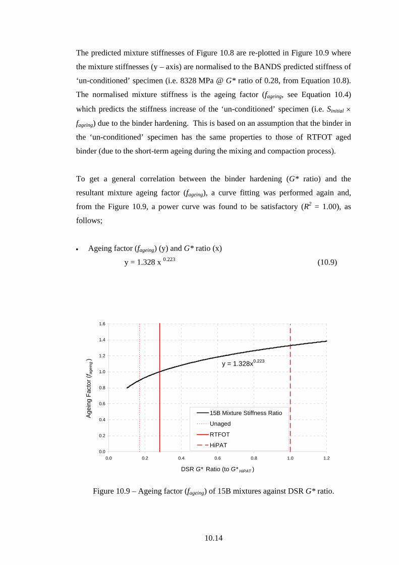
10.14

The predicted mixture stiffnesses of Figure 10.8 are re-plotted in Figure 10.9 where

the mixture stiffnesses (y – axis) are normalised to the BANDS predicted stiffness of

‘un-conditioned’ specimen (i.e. 8328 MPa @ G* ratio of 0.28, from Equation 10.8).

The normalised mixture stiffness is the ageing factor (fageing, see Equation 10.4)

which predicts the stiffness increase of the ‘un-conditioned’ specimen (i.e. Sinitial ×

fageing) due to the binder hardening. This is based on an assumption that the binder in

the ‘un-conditioned’ specimen has the same properties to those of RTFOT aged

binder (due to the short-term ageing during the mixing and compaction process).

To get a general correlation between the binder hardening (G* ratio) and the

resultant mixture ageing factor (fageing), a curve fitting was performed again and,

from the Figure 10.9, a power curve was found to be satisfactory (R2 = 1.00), as

follows;

• Ageing factor (fageing) (y) and G* ratio (x)

y = 1.328 x 0.223 (10.9)

y = 1.328x0.223

0.0

0.2

0.4

0.6

0.8

1.0

1.2

1.4

1.6

0.0 0.2 0.4 0.6 0.8 1.0 1.2

DSR G* Ratio (to G* HiPAT )

Age

ing

Fact

or (f

agei

ng)

15B Mixture Stiffness Ratio

Unaged

RTFOT

HiPAT

Figure 10.9 – Ageing factor (fageing) of 15B mixtures against DSR G* ratio.

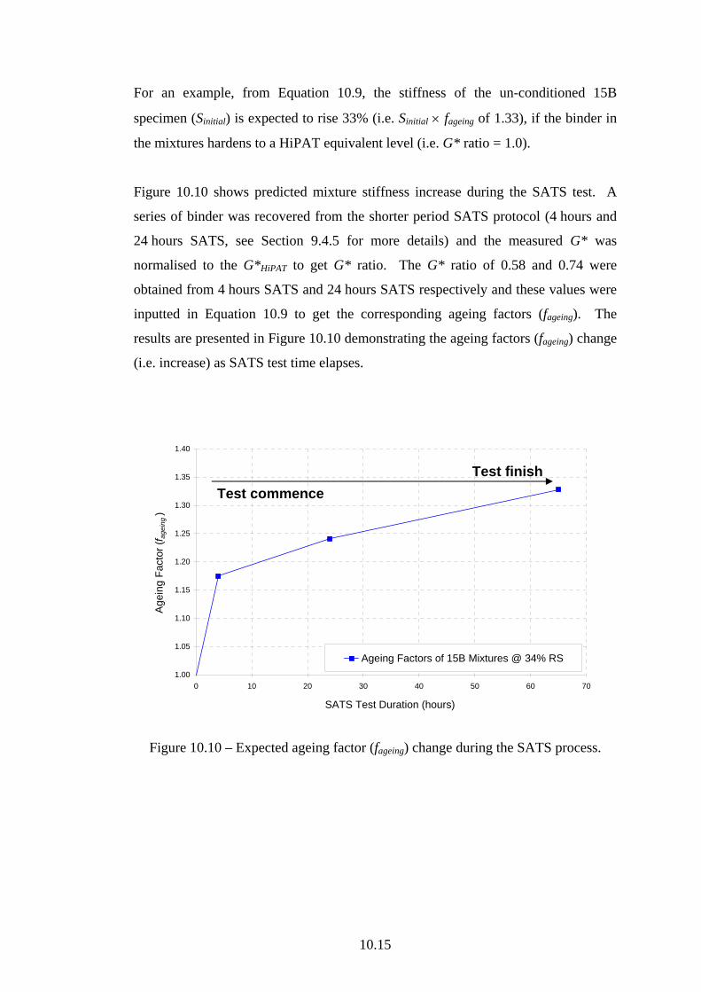
10.15

For an example, from Equation 10.9, the stiffness of the un-conditioned 15B

specimen (Sinitial) is expected to rise 33% (i.e. Sinitial × fageing of 1.33), if the binder in

the mixtures hardens to a HiPAT equivalent level (i.e. G* ratio = 1.0).

Figure 10.10 shows predicted mixture stiffness increase during the SATS test. A

series of binder was recovered from the shorter period SATS protocol (4 hours and

24 hours SATS, see Section 9.4.5 for more details) and the measured G* was

normalised to the G*HiPAT to get G* ratio. The G* ratio of 0.58 and 0.74 were

obtained from 4 hours SATS and 24 hours SATS respectively and these values were

inputted in Equation 10.9 to get the corresponding ageing factors (fageing). The

results are presented in Figure 10.10 demonstrating the ageing factors (fageing) change

(i.e. increase) as SATS test time elapses.

Figure 10.10 – Expected ageing factor (fageing) change during the SATS process.

1.00

1.05

1.10

1.15

1.20

1.25

1.30

1.35

1.40

0 10 20 30 40 50 60 70

SATS Test Duration (hours)

Age

ing

Fact

or (f

agei

ng)

Ageing Factors of 15B Mixtures @ 34% RS

Test commence Test finish

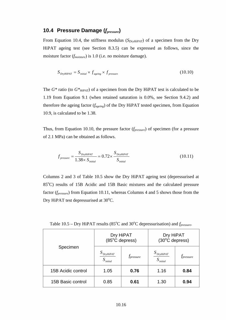
10.16

10.4 Pressure Damage (fpressure)

From Equation 10.4, the stiffness modulus (SDryHiPAT) of a specimen from the Dry

HiPAT ageing test (see Section 8.3.5) can be expressed as follows, since the

moisture factor (fmoisture) is 1.0 (i.e. no moisture damage).

pressureageinginitialDryHiPAT ffSS ××= (10.10)

The G* ratio (to G*HiPAT) of a specimen from the Dry HiPAT test is calculated to be

1.19 from Equation 9.1 (when retained saturation is 0.0%, see Section 9.4.2) and

therefore the ageing factor (fageing) of the Dry HiPAT tested specimen, from Equation

10.9, is calculated to be 1.38.

Thus, from Equation 10.10, the pressure factor (fpressure) of specimen (for a pressure

of 2.1 MPa) can be obtained as follows.

initial

DryHiPAT

initial

DryHiPATpressure S

SS

Sf ×=

×= 72.0

38.1 (10.11)

Columns 2 and 3 of Table 10.5 show the Dry HiPAT ageing test (depressurised at

85oC) results of 15B Acidic and 15B Basic mixtures and the calculated pressure

factor (fpressure) from Equation 10.11, whereas Columns 4 and 5 shows those from the

Dry HiPAT test depressurised at 30oC.

Table 10.5 – Dry HiPAT results (85oC and 30oC depressurisation) and fpressure.

Dry HiPAT (85oC depress)

Dry HiPAT (30oC depress)

Specimen

initial

DryHiPAT

SS

fpressure initial

DryHiPAT

SS

fpressure

15B Acidic control 1.05 0.76 1.16 0.84

15B Basic control 0.85 0.61 1.30 0.94

10.17

Table 10.5 clearly demonstrates that Basic mixture has more pressure damage (i.e.

lower fpressure) than that of Acidic mixture, from 85oC depressurisation Dry HiPAT

test. However, the pressure damage of Basic mixture was much reduced (i.e. higher

fpressure) by depressurising at 30oC, suggesting that the modified SATS protocol

(depressurising at 30oC, see Section 8.3) can significantly reduce the pressure

damage, as proposed.

10.5 Moisture Sensitivity (fmoisture) of SATS Data

From the Shell BANDS 2.0 software and the Dry HiPAT ageing test, the ageing

factor (fageing) and the pressure factor (fpressure) have been identified respectively. For

examples, if a specimen shows an initial stiffness of 10,000 MPa (Sinitial) and a

conditioned stiffness of 5,000 MPa after the SATS test (Sconditioned), the nominal

retained stiffness of the specimen (RSnominal) is calculated to be 0.50 (5,000 MPa /

10,000 MPa), from Equation 10.3. However, from Equations 10.5 and 10.9, the

‘true’ moisture sensitivity (fmoisture) of the specimen is calculated as follows, if the

binder in the specimen was aged to HiPAT equivalent level (i.e. G* ratio = 1.0) and

tested using the standard SATS, for 15B Acidic specimens (fpressure = 0.76);

49.076.033.1000,10

000,5=

××=moisturef

For 15B Basic specimens (fpressure = 0.61),

62.061.033.1000,10

000,5=

××=moisturef

If the specimen was tested using the modified SATS, for 15B Acidic specimens

(fpressure = 0.84),

45.084.033.1000,10

000,5=

××=moisturef

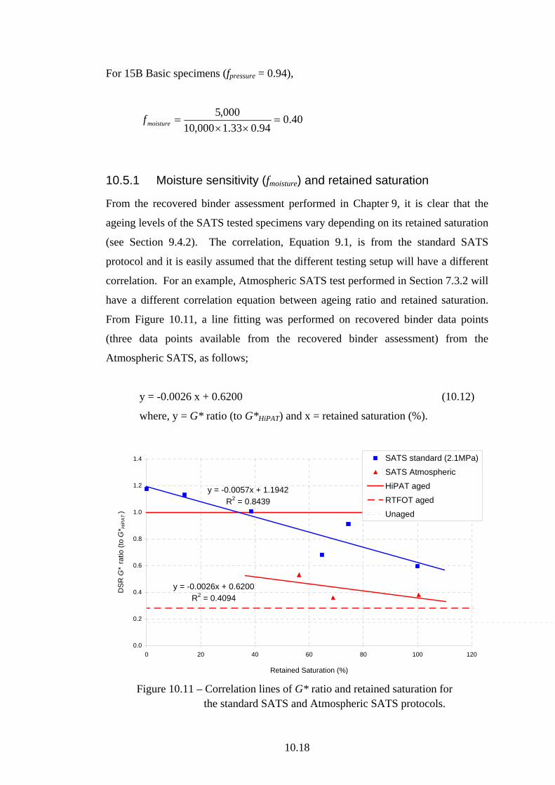
10.18

For 15B Basic specimens (fpressure = 0.94),

40.094.033.1000,10

000,5=

××=moisturef

10.5.1 Moisture sensitivity (fmoisture) and retained saturation

From the recovered binder assessment performed in Chapter 9, it is clear that the

ageing levels of the SATS tested specimens vary depending on its retained saturation

(see Section 9.4.2). The correlation, Equation 9.1, is from the standard SATS

protocol and it is easily assumed that the different testing setup will have a different

correlation. For an example, Atmospheric SATS test performed in Section 7.3.2 will

have a different correlation equation between ageing ratio and retained saturation.

From Figure 10.11, a line fitting was performed on recovered binder data points

(three data points available from the recovered binder assessment) from the

Atmospheric SATS, as follows;

y = -0.0026 x + 0.6200 (10.12)

where, y = G* ratio (to G*HiPAT) and x = retained saturation (%).

y = -0.0026x + 0.6200R2 = 0.4094

y = -0.0057x + 1.1942R2 = 0.8439

0.0

0.2

0.4

0.6

0.8

1.0

1.2

1.4

0 20 40 60 80 100 120

Retained Saturation (%)

DS

R G

* ra

tio (t

o G

* HiP

AT)

SATS standard (2.1MPa)

SATS Atmospheric

HiPAT aged

RTFOT aged

Unaged

Figure 10.11 – Correlation lines of G* ratio and retained saturation for the standard SATS and Atmospheric SATS protocols.

10.19

Equations 9.1 (for standard SATS) and 10.12 (for Atmospheric SATS) have been

used to produce a master chart, Figure 10.12, showing ageing factor and pressure

factor (i.e. fageing × fpressure) according to the material type (15B Acidic and Basic),

testing conditions (standard SATS and Atmospheric SATS) and corresponding

retained saturations. It should be noted that the pressure factor (fpressure) of

Atmospheric SATS is 1.0 (i.e. no pressure damage), thus fageing × fpressure = fageing.

Separate curve fittings were performed and a 2nd order polynomial was found to be

satisfactory for each case (R2 > 0.99). The correlations for 15B Acidic and 15B

Basic from the standard SATS are expressed in Equations in 10.13 and 10.14,

respectively. The correlation for Atmospheric SATS is expressed in Equation 10.15,

as follows;

y = -0.000004 x2 – 0.001007 x + 1.048922 (10.13)

y = -0.000003 x2 – 0.000808 x + 0.841898 (10.14)

y = -0.000003 x2 – 0.001041 x + 1.192980 (10.15)

where, y = fageing × fpressure, and x = retained saturation (%).

Figure 10.13 presents another master chart showing ageing and pressure factor (i.e.

fageing × fpressure) of 15B Acidic and 15B Basic specimens from the modified SATS

protocol. The same ageing factor (fageing) of standard SATS (i.e. using Equations 9.1

and 10.9) was directly applied to the modified SATS and the pressure factors

(fpressure) were from Table 10.5 (from Dry HiPAT 30oC depressurisation test).

The correlations for 15B Acidic and 15B Basic from the modified SATS are

expressed in Equations in 10.16 and 10.17, respectively.

y = -0.000004 x2 – 0.001113 x + 1.159335 (10.16)

y = -0.000005 x2 – 0.001245 x + 1.297351 (10.17)

where, y = fageing × fpressure, and x = retained saturation (%).

10.20

Figure 10.12 – Master chart showing fageing × fpressure of standard SATS

and Atmospheric SATS.

y = -0.000004x2 - 0.001113x + 1.159335

y = -0.000005x2 - 0.001245x + 1.297351

0.0

0.2

0.4

0.6

0.8

1.0

1.2

1.4

1.6

0 20 40 60 80 100 120

Retained Saturation (%)

f age

ing

x f p

ress

ure

15B Acidic modified SATS

15B Basic modified SATS

Figure 10.13 – Master chart showing fageing × fpressure of modified SATS

y = -0.000004x2 - 0.001007x + 1.048922

y = -0.000003x2 - 0.000808x + 0.841898

y = -0.000003x2 - 0.001041x + 1.192980

0.0

0.2

0.4

0.6

0.8

1.0

1.2

1.4

1.6

0 20 40 60 80 100 120

Retained Saturation (%)

f age

ing

x f p

ress

ure

15B Acidic standard SATS

15B Basic standard SATS

15B Atmospheric SATS

Atmospheric SATS fpressure = 1.0

10.21

For examples, if a specimen shows an initial stiffness of 10,000 MPa and a

conditioned stiffness of 5,000 MPa (i.e. RSnominal = 0.5) with a retained saturation of

50%, the ageing and pressure factors (fageing × fpressure) of the specimen are calculated,

as follows;

• 15B Acidic standard SATS → 0.99 (from Equation 10.13),

• 15B Basic standard SATS → 0.79 (from Equation 10.14),

• 15B Atmospheric SATS → 1.13 (from Equation 10.15),

• 15B Acidic modified SATS → 1.09 (from Equation 10.16), and

• 15B Basic modified SATS → 1.22 (from Equation 10.17).

Thus, from Equation 10.5, the ‘true’ moisture sensitivity (fmoisture) of the specimen is

calculated, as follows;

• 15B Acidic standard SATS → 0.51,

• 15B Basic standard SATS → 0.64,

• 15B Atmospheric SATS → 0.44,

• 15B Acidic modified SATS → 0.46, and

• 15B Basic modified SATS → 0.41.

This generally agrees that, Atmospheric SATS and the modified SATS have

relatively severer moisture damage condition than that of standard SATS. This is

assumed to be due to a more accelerated water circulation of Atmospheric SATS

10.22

(see Section 7.3 for more discussions), and due to the increased and prolonged water

contact of the modified SATS (see Section 8.3.1 for more discussions).

Figure 10.14 shows typical examples of retained stiffness (RSnominal) and moisture

sensitivity (fmoisture) of the 15B Acidic material tested using the standard,

Atmospheric or modified SATS.

Figure 10.14 – Examples of retained stiffness (RSnominal) and moisture sensitivity

(fmoisture) of 15B Acidic material.

As observed in Figure 10.14, fmoisture of 15B Acidic material commonly show

relatively lower values than its RSnominal, although the difference is very marginal

(virtually identical values for the standard SATS).

Figure 10.15 shows typical examples of retained stiffness (RSnominal) and moisture

sensitivity (fmoisture) of the 15B Basic material tested using the standard, Atmospheric

or modified SATS.

0.0

0.2

0.4

0.6

0.8

1.0

1.2

0 20 40 60 80 100 120

Retained Saturation (%)

f moi

stur

e an

d R

etai

ned

stiff

enss

15B Acidic RS standard SATS

15B Acidic fm standard SATS

15B Acidic RS Atmospheric SATS

15B Acidic fm Atmospheric SATS

15B Acidic RS modified SATS

15B Acidic fm modified SATS

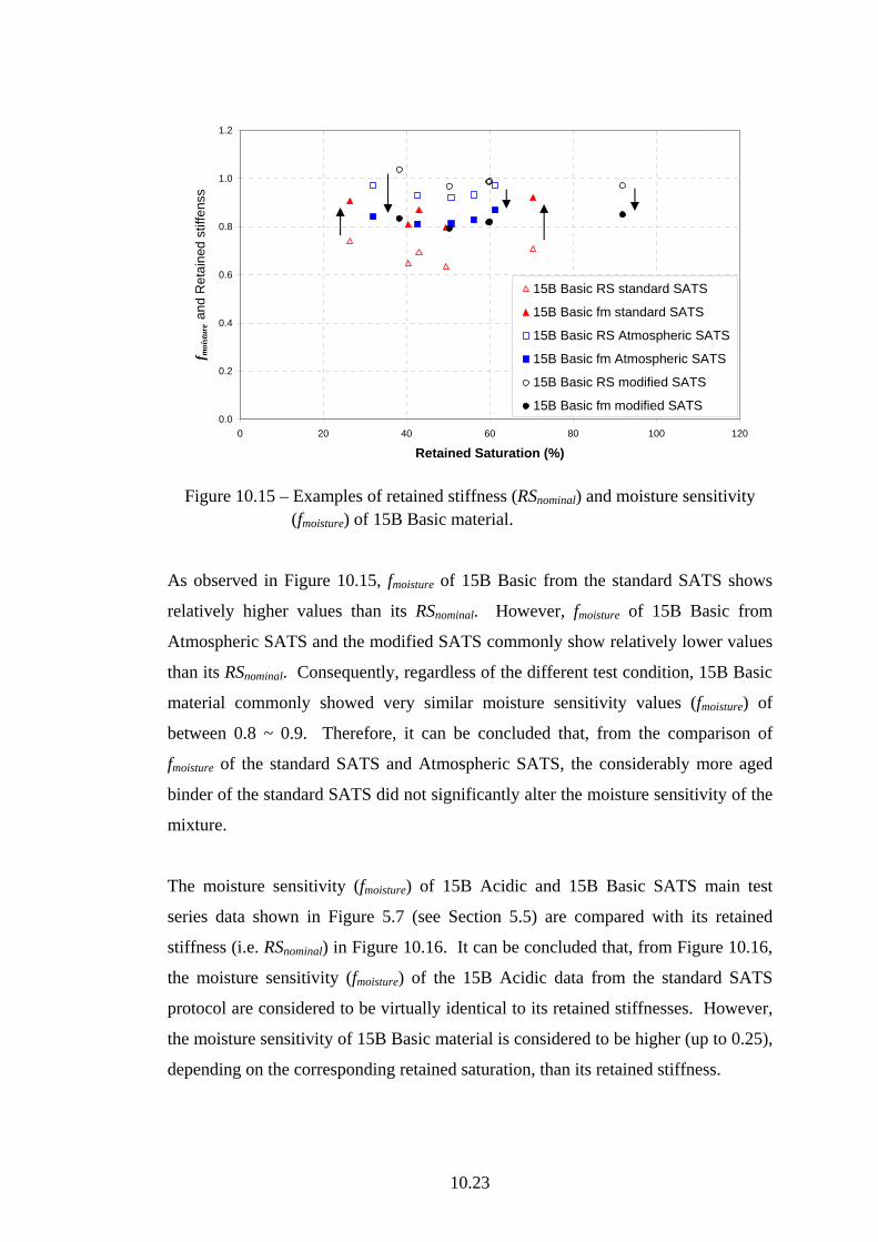
10.23

Figure 10.15 – Examples of retained stiffness (RSnominal) and moisture sensitivity

(fmoisture) of 15B Basic material.

As observed in Figure 10.15, fmoisture of 15B Basic from the standard SATS shows

relatively higher values than its RSnominal. However, fmoisture of 15B Basic from

Atmospheric SATS and the modified SATS commonly show relatively lower values

than its RSnominal. Consequently, regardless of the different test condition, 15B Basic

material commonly showed very similar moisture sensitivity values (fmoisture) of

between 0.8 ~ 0.9. Therefore, it can be concluded that, from the comparison of

fmoisture of the standard SATS and Atmospheric SATS, the considerably more aged

binder of the standard SATS did not significantly alter the moisture sensitivity of the

mixture.

The moisture sensitivity (fmoisture) of 15B Acidic and 15B Basic SATS main test

series data shown in Figure 5.7 (see Section 5.5) are compared with its retained

stiffness (i.e. RSnominal) in Figure 10.16. It can be concluded that, from Figure 10.16,

the moisture sensitivity (fmoisture) of the 15B Acidic data from the standard SATS

protocol are considered to be virtually identical to its retained stiffnesses. However,

the moisture sensitivity of 15B Basic material is considered to be higher (up to 0.25),

depending on the corresponding retained saturation, than its retained stiffness.

0.0

0.2

0.4

0.6

0.8

1.0

1.2

0 20 40 60 80 100 120

Retained Saturation (%)

f moi

stur

e an

d R

etai

ned

stiff

enss

15B Basic RS standard SATS

15B Basic fm standard SATS

15B Basic RS Atmospheric SATS

15B Basic fm Atmospheric SATS

15B Basic RS modified SATS

15B Basic fm modified SATS

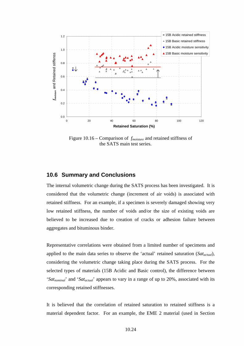
10.24

Figure 10.16 – Comparison of fmoisture and retained stiffness of

the SATS main test series.

10.6 Summary and Conclusions

The internal volumetric change during the SATS process has been investigated. It is

considered that the volumetric change (increment of air voids) is associated with

retained stiffness. For an example, if a specimen is severely damaged showing very

low retained stiffness, the number of voids and/or the size of existing voids are

believed to be increased due to creation of cracks or adhesion failure between

aggregates and bituminous binder.

Representative correlations were obtained from a limited number of specimens and

applied to the main data series to observe the ‘actual’ retained saturation (Satactual),

considering the volumetric change taking place during the SATS process. For the

selected types of materials (15B Acidic and Basic control), the difference between

‘Satnominal’ and ‘Satactual’ appears to vary in a range of up to 20%, associated with its

corresponding retained stiffnesses.

It is believed that the correlation of retained saturation to retained stiffness is a

material dependent factor. For an example, the EME 2 material (used in Section

0.0

0.2

0.4

0.6

0.8

1.0

1.2

0 20 40 60 80 100 120

Retained Saturation (%)

f moi

stur

e an

d R

etai

ned

stiff

enss

15B Acidic retained stiffness

15B Basic retained stiffness

15B Acidic moisture sensitivity

15B Basic moisture sensitivity

10.25

6.4.1) is likely to have a different correlation equation, as it has different volumetric

properties. However, it still can be believed that the less damaged specimens (higher

retained stiffness) will have less volumetric change. For an example, the EME 2

specimens tested in Section 6.4.1, which showed relatively low retained stiffness

with clearly visible expansion of specimen size, will have higher volumetric change,

while the identical specimens tested in Section 8.3.3 (using the modified SATS) will

have much less volumetric change.

The ‘true’ moisture sensitivity (i.e. fmoisture) of the material from the SATS protocol

has been investigated (by extracting ageing factor and pressure factor). The

correlation between binder ageing (G* ratio) and the expected mixture stiffness

increase (i.e. fageing) has been obtained using the Shell BANDS 2.0 software. The

correlation has been used to predict stiffness increase curve for the 15B materials

(only by fageing) and, from this curve, the pressure damage (i.e. fpressure) caused by the

applied high pressure of the SATS protocol has been identified. Consequently, the

moisture sensitivity of the material used in this thesis has been identified.

From the investigation of the ‘true’ moisture sensitivity which showed very similar

values regardless of different binder ageing level (especially from 15B Basic

mixture), it can be concluded that, for the limited material range covered in this

study, the ageing of the binder did not significantly alter the moisture sensitivity of

the mixture.

11.1

Chapter 11. Summary, Conclusions and Recommendations for Future Work

11.1 General Summary

Due to concerns over ageing and moisture sensitivity of HMB materials, from on-

going monitoring of the initial trial site, a research programme was established to

investigate the long-term durability of the material. The main objective of the

research programme was to develop a laboratory testing procedure able to reproduce

the material properties observed in the HMB trial site, with a specific interest in the

ageing and moisture sensitivity combined long-term durability of the HMB

materials.

Since none of the existing durability protocols are found to be able (or designed) to

do the purpose, the prime concern was given to develop a new protocol which would

combine the effect of the both aspects (ageing and water damage) together in one

process. More specifically, the protocol needs to be able to simulate 60% or more

reduction in mixture stiffness due to moisture damage, combined with 10 or more

years of ‘long-term’ binder ageing.

11.1.1 Literature review (Chapter 2)

The main aim of the literature review was to provide the reader with the relevant

background knowledge applicable to this study (particularly durability test methods).

Therefore, the chapter was divided into three main sections reviewing ‘Introduction

to Pavement Engineering’, ‘Ageing Tests for Bituminous Materials’ and ‘Moisture

Sensitivity Tests for Bituminous Materials’.

The binder ageing can be divided into short and long term ageing. The ‘short-term’

describes that the ageing process (mainly volatile loss) occurred during the asphalt

mixture construction process (heating up, mixing, delivery and compaction) and the

‘long-term’ describes that the progressive oxidation process of the in-place material

in the field during its service life.

11.2

Moisture sensitivity tests generally have a conditioning and an evaluation phase.

The conditioning processes associated with most test methods are to simulate the

deterioration of the asphalt mixture in the field exposure conditions, in an

accelerated manner to be tested in a reasonably shorter periods of time. Normally

the acceleration is achieved by immersing the material in an elevated temperature.

Most moisture sensitivity test procedures on the compacted mixture measure the loss

of strength and stiffness of an asphalt mixture due to moisture conditioning. The

most common way of quantifying the damage caused by the conditioning process is

to directly compare the ‘conditioned’ mechanical properties to those of

‘unconditioned’. The mechanical properties can be evaluated using various

mechanical tests which can be divided into destructive (compression, stability,

indirect tensile strength and fatigue) and non-destructive (indirect tensile stiffness

and resilient modulus) approaches.

11.1.2 Development of SATS Protocol (Chapters 3 and 4)

Chapter 3 presented a series of preliminary tests. Among the various trials

investigated in this chapter, to find a suitable durability test method which fulfils the

given objectives of this study, the HiPAT ageing using vacuum saturated specimens

showed the most interesting behaviour. Firstly it was the only process which was

severe enough to produce the target stiffness reduction within reasonably shorter

period of time. Secondly it was the only process which had ageing and moisture

sensitivity schemes in ‘one process’.

The investigation on the recovered binder extracted from the specimens which had

been through the above protocol (referred to as preliminary SATS) clearly

demonstrated a comparable level of binder ageing to the HiPAT aged binder.

Knowing that the binder in the mixture will be ‘long-term’ aged according to the

given HiPAT ageing conditions, while the compacted specimens are ‘moisture

damaged’ by saturated water in the pressure vessel, the SATS protocol showed a

strong possibility to be a suitable durability test method which fulfils the given

objectives of the study.

11.3

Chapter 4 described the details of SATS protocol development procedure. The

preliminary version of SATS protocol (preliminary SATS) was performed on

laboratory manufactured specimens. The variability investigation using nominally

identical sets of specimens revealed that the test conditions vary dependent on the

specimen position within the vessel and the key factor is believed to be the retained

saturation.

Among the various modifications to optimise the SATS protocol, considering the

practicability and repeatability of the protocol, the semi immersion SATS protocol

appeared to be the most suitable approach, as it produces from a very dry specimen

to a completely immersed specimen with gradually saturated specimens between

them.

11.1.3 SATS Durability Test (Chapters 5 and 6)

Chapter 5 presented SATS durability tests results performed on a series of mixtures

including a mixture nominally identical to that used in the HMB trial site. Generally

the Basic mixture series showed a better performance than the Acidic mixture series.

For Acidic aggregate mixture series the retained stiffness (at a particular retained

saturation) was compared favourably with the stiffness modulus reduction observed

from the initial trial site.

An investigation of test variability showed a reasonably good repeatability with the

mixtures selected. No statistically clear difference was found from nominally

identical mixtures that contained binders from different sources. The retained

saturation variation at each specimen position was also investigated and generally

showed a practically acceptable range of variation.

Chapter 6 presented the SATS test results performed on a wider range of mixtures.

The results from Acidic mixtures with HLF showed superior performances.

However, the already good performance of the Basic mixtures was not significantly

improved by the adding of HLF. The effect of anti-stripping agent was also

investigated and showed some improved performance.

11.4

Investigation on mixture variability showed an unexpected results showing well

compacted or richer mixture performing poorer than the control mixture, especially

for the Basic mixtures. 15E Basic EME material also showed worse performance

than expected.

11.1.4 SATS Parameters and Modification (Chapters 7 and 8)

Chapter 7 presented a more carefully investigation on the parameters used in the

SATS protocol. It appears that the applied pressure, to induce the accelerate binder

ageing, is also inducing a certain degree of specimen damage. Consequently two

different modes of pressure related damage were proposed and their expected

properties are suggested.

Chapter 8 described the modified SATS protocol which was developed to reduce the

pressure damage observed in the previous chapters. The modified SATS protocol

was applied to a limited range of mixtures and clearly displayed much reduced level

of pressure damage (especially from the Basic mixture series).

11.1.5 Recovered Binder Assessment (Chapter 9)

Chapter 9 presented an extensive investigation on recovered binders from various

SATS conditions. Comparison of saturated SATS and dry SATS test showed similar

level of ageing regardless of the existence of water. However, the fully immersed

specimen from the standard SATS and Atmospheric SATS commonly showed much

less level of ageing compared to the specimens above the water level from the

standard SATS.

A more careful investigation on the ageing variation along the specimen position

revealed that there is a clear trend of ageing level dependent on the specimen

position. From a limited set of results a representative line was fitted and a retained

saturation of 34% was found to be the HiPAT equivalent ageing condition for the

15B Acidic standard mixture from the standard SATS protocol.

11.5

11.1.6 Data Interpretation (Chapter 10)

Chapter 10 presented a further investigation to interpret the nominal SATS data

obtained in the previous chapters more accurately. The internal volumetric change

during the SATS process was investigated. It was considered that the volumetric

change is associated with retained stiffnesses. Representative correlations were

obtained from a limited number of specimens and applied to the main data series to

observe the ‘actual’ retained saturation (i.e. Satactual), considering the volumetric

change during the SATS test process.

The ‘true’ moisture sensitivity (fmoisture), by extracting the ageing factor (fageing) and

pressure factor (fpressure), was investigated. The correlation between binder ageing

(expressed in G* ratio to G*HiPAT) and the ageing factor (i.e. stiffness increase due to

binder ageing in the mixture) was obtained using the Shell BANDS 2.0 software.

The ageing factor was used to predict ‘un-damaged’ stiffness increment curve for the

15B materials, and from this curve, the pressure factor (i.e. stiffness reduction caused

by the applied high pressure of the SATS protocol) was identified. Consequently the

‘true’ moisture sensitivity (i.e. stiffness reduction caused by the moisture damage

only) of the material was obtained and compared to the ‘nominal’ retained stiffness.

11.2 Conclusions

The following conclusions have been drawn from the various chapters of this thesis.

• From the worldwide questionnaire survey (Appendix B), the most commonly

used tests for short-term and long-term ageing simulation are the RTFOT and

PAV protocols respectively.

• A temperature of 85oC appears to be the maximum applicable temperature to age

the compacted specimen.

• The existing durability protocols are designed to investigate one aspect only (i.e.

ageing test for ageing sensitivity, moisture sensitivity test for moisture damage).

11.6

• In long-term service condition, pavements undergo both aspects of ageing and

moisture damage together (i.e. materials damaged by water infiltration while the

binder in the material is being aged).

• Binder of the HiPAT aged specimen is expected to be aged comparable to the

HiPAT aged binder, regardless of existence of moisture in the pressure vessel.

• The retained saturation is the key factor to control the magnitude of damage

created by the SATS protocol.

• In the SATS test setup, the retained saturation variation depending on the

specimen position is inevitable and therefore needs to be accepted as a test

parameter.

• Retained saturation variation depending on the specimen position in the pressure

vessel is beneficial since the sensitivity of a material to the various amount of

moisture could be obtained.

• For the mixture range investigated in Chapter 5, the SATS protocol successfully

discriminated the durability of mixtures against the combined effect of ageing

and moisture damage, on the basis of a measured reduction in stiffness similar to

that observed in the initial HMB trial site.

• Variability investigation on the SATS protocol showed a practically acceptable

level of variation of retained stiffnesses and retained saturations.

• The high pressure applied to accelerate the ageing process of binder in the

compacted specimens also induces a certain degree of damage (stiffness

reduction) to the specimen.

• The pressure damage mainly occurs during the depressurising process.

• Magnitude of the pressure damage is closely related to the proportion of Mode I

(deformation) and Mode II (puncture) damage.

11.7

• A mixture with a higher binder content and/or lower air voids is more susceptible

to the pressure damage from the SATS protocol, as the mixture is likely to have a

more closed ‘non-interconnected’ voids.

• A mixture with a better adhesion property between aggregates and binder is

likely more susceptible to the pressure damage as the mixture will create more

‘non-interconnected’ voids along the interface of aggregates and binder.

• A mixture with a softer binder is thought to be more susceptible to the pressure

damage as the binder will have more viscose properties at a same pressurising (or

depressurising) temperature.

• Considering the distinctively ‘lean’ volumetric properties of the materials

focused on this study, the SATS data produced in Chapter 5 using various

combinations of binders and aggregates are considered to be credible, especially

for the Acidic materials which are nominally identical to the HMB trial site

material.

• For the Basic materials, the presented data in Chapter 5 incorporates a

considerable amount of pressure damage and the damage can be reduced by the

modified SATS protocol.

• The modified SATS protocol, presented in Chapter 8, is a better protocol,

especially to be applied to a wider range of mixtures including the mixtures with

more pressure sensitive volumetric properties.

• For the 15B Granite mixtures the ageing level of binder in the standard SATS

tested specimens varies depending on its retained saturation and the HiPAT

binder equivalent ageing can be found in a retained saturation of 34%.

• To achieve a HiPAT equivalent binder ageing from the SATS protocol within the

same testing duration (65 hours), the pressure and temperature conditions

(2.1 MPa and 85oC) used in the standard SATS are necessary.

11.8

• Initial volumetric properties of the specimen can change during the SATS

process, and can be correlated to its retained stiffness.

• The retained stiffness used to present SATS test results is a combined function of

ageing factor, pressure factor and moisture factor.

• By extracting the ageing factor and pressure factor, the moisture sensitivity of the

material from the SATS test can be identified.

• From the limited material range covered in this study, the ageing of the binder

did not significantly alter the moisture sensitivity of the mixture.

• Considering the variability of the SATS test and the pressure damage

incorporated, materials tested using the SATS protocol need to be ranked in a

broad range.

• From the limited range of materials observed in this study, the following

guideline of durability performance can be suggested (in a retained saturation

range higher than 40%).

• A (Retained stiffness > 0.8) – excellent performance.

• B (0.8 > Retained stiffness > 0.4) – acceptable performance.

• C (Retained stiffness < 0.4) – poor performance.

11.3 Recommendations for Future Work

For this thesis, the standard SATS (presented in Chapter 5) was the main testing

protocol under investigation. However, from the findings in the later stage, the

modified SATS (30oC depressurising) clearly demonstrated to be a better and more

recommendable protocol (in Chapter 8). Thus the modified SATS protocol needs to

be accepted as ‘the’ SATS protocol (instead of the standard SATS). Consequently,

to understand the test variability and recovered binder properties of the modified

SATS protocol, the variability investigation performed in Chapter 5 and the

11.9

recovered binder assessment performed in Chapter 9 are recommended to be

performed on the modified SATS protocol as the same manners.

The performance ranking guideline proposed in the previous section is only an

example, based on a limited range of HMB materials covered in this study. A more

credible and acceptable guideline can only be produced by testing of a much wider

range of HMB mixtures, desirably linked with the field performance.

Since the prime objective of the research presented in this thesis was to reproduce

the material properties observed in the initial HMB trial site, it was inevitable to

produce a testing protocol specifically focused on a particular material type (i.e.

HMB with lean volumetric properties). Although this initial goal has been

successfully achieved, it is still desirable for the protocol to be applicable to a wider

range of mixture types. Thus mixtures with relatively softer binders (e.g. 25 Pen and

35 Pen grade binders) need to be investigated to find the limit of the applicability of

the SATS protocol. Also more various types of aggregates and gradings need to be

reviewed.

The correlation of retained saturation and retained stiffness obtained in Chapter 10

was based on a limited number of specimens only. Thus to make the correlations

more accurate and credible, a more number of specimens needs to be investigated.

Also it should be noted that only the control specimens (i.e. 15B Acidic/Basic with

High AV/Low BC) were observed in this investigation. Since mixtures with

different properties (e.g. Low AV, High BC or EME material) are expected to have

different correlation curves, it is desirable to observe the volumetric change of such

materials, as the same manner used for the control mixtures.

The correlation of binder hardening and resultant mixture stiffness increase was

estimated based on the nomographs produced using different range of materials and

testing conditions to those used in this study. Thus it is desirable to produce the

correlation using the identical material and testing conditions used in this study.

This can be achieved by a series of investigation on recovered binders from

conventional dry oven aged specimens (identical mixtures used in this study) under

various ageing period. This investigation can also be used to find an identical oven

11.10

ageing time equivalent to the HiPAT binder ageing protocol without the pressure

factor. Ultimately this investigation can lead to develop an alternative SATS

protocol without concerns on pressure damage. Although a much longer testing time

is expected, the alternative protocol can effectively be used as a comparison protocol

to the SATS protocol developed in this study.

Appendix A - Core Logs from HMB Field Site

(Selected examples of cores in poor,

intermediate and good conditions)

Appendix B – Questionnaire Survey of Durability Tests on Bituminous Material

Appendix C – Binder Characterisation Tests - Penetration Test

- Softening Point Test

- Rotational Viscosity Test

- Dynamic Shear Rheometer Test

Appendix D – Draft of SATS Protocol

Note: 1. This protocol is referred to as ‘standard SATS’ in the main chapters. 2. The term ‘retained stiffness’ used in the main chapters is referred to as

‘Stiffness Ratio’ 3. The term ‘retained saturation’ used in the main chapters is referred to as

‘Saturation after Conditioning’.

Appendix E – Individual Test Data Charts

Appendix F – Manual of Contracted Document for Highway Works: Clause 953

Method for the Assessment of Durability of Compacted Asphalt

Mixtures using the Saturation Ageing Tensile Stiffness (SATS) Test

Note: 1. This protocol is referred to as ‘modified SATS’ in the main chapters. 2. The term ‘retained stiffness’ used in the main chapters is referred to as

‘Stiffness Ratio’ 3. The term ‘retained saturation’ used in the main chapters is referred to as

‘Saturation after Conditioning’.

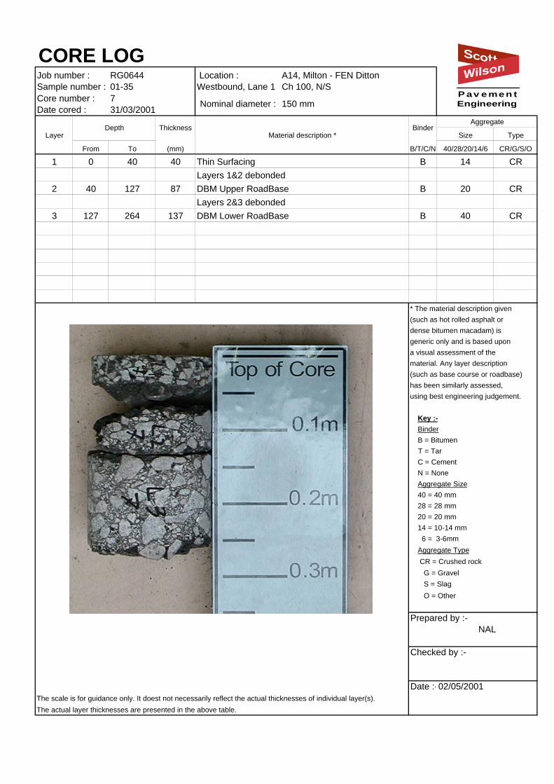
Job number : RG0644 Location : A14, Milton - FEN DittonSample number : 01-35 Westbound, Lane 1 Ch 100, N/SCore number : 7Date cored : 31/03/2001

Layer Size Type

From To (mm) B/T/C/N 40/28/20/14/6 CR/G/S/O

1 0 40 40 Thin Surfacing B 14 CRLayers 1&2 debonded

2 40 127 87 DBM Upper RoadBase B 20 CRLayers 2&3 debonded

3 127 264 137 DBM Lower RoadBase B 40 CR

* The material description given(such as hot rolled asphalt or dense bitumen macadam) is generic only and is based upona visual assessment of thematerial. Any layer description(such as base course or roadbase)has been similarly assessed,using best engineering judgement.

Key :-BinderB = Bitumen

T = TarC = CementN = NoneAggregate Size40 = 40 mm28 = 28 mm20 = 20 mm14 = 10-14 mm 6 = 3-6mmAggregate Type CR = Crushed rock G = Gravel S = Slag O = Other

Prepared by :-

Checked by :-

Date :-02/05/2001The scale is for guidance only. It doest not necessarily reflect the actual thicknesses of individual layer(s).The actual layer thicknesses are presented in the above table.

NAL

Aggregate

CORE LOG

Depth Thickness BinderMaterial description *

Nominal diameter : 150 mmP av emen tEngineering

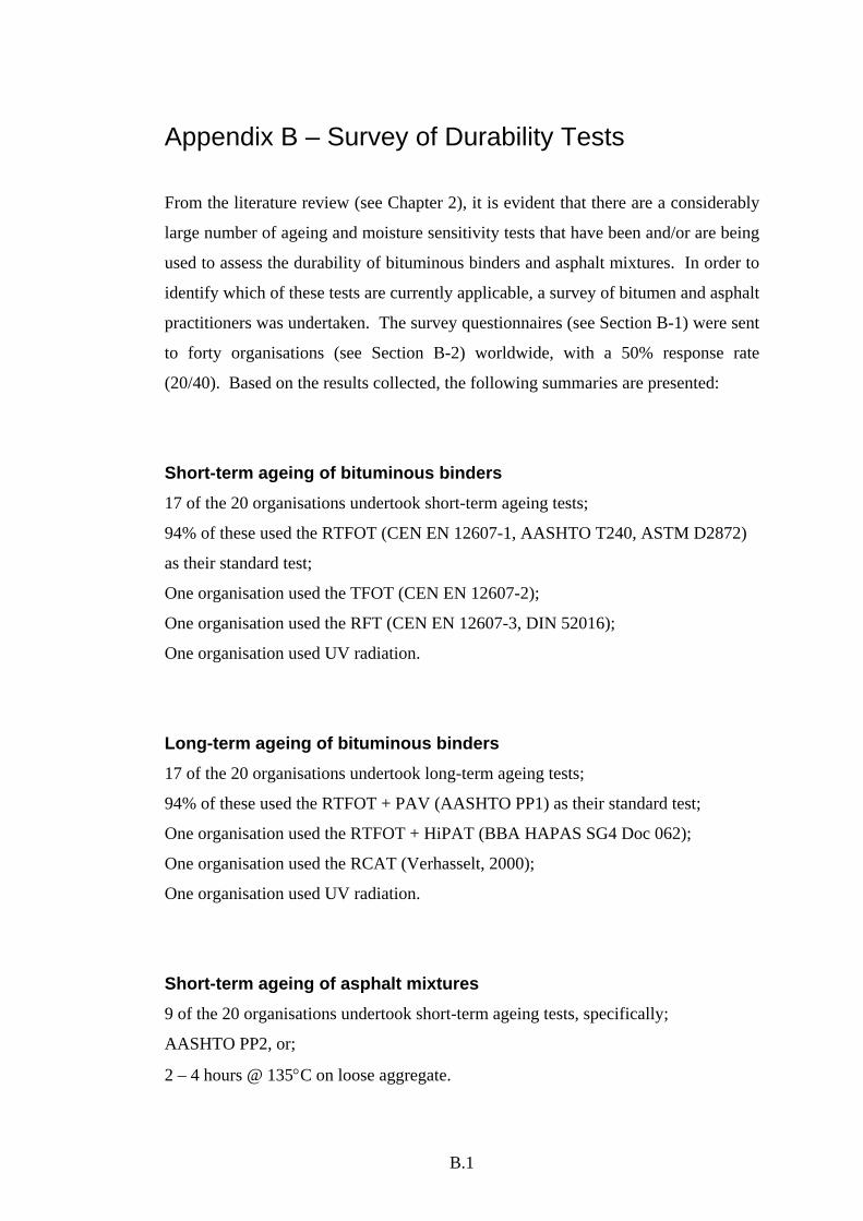
B.1

Appendix B – Survey of Durability Tests

From the literature review (see Chapter 2), it is evident that there are a considerably

large number of ageing and moisture sensitivity tests that have been and/or are being

used to assess the durability of bituminous binders and asphalt mixtures. In order to

identify which of these tests are currently applicable, a survey of bitumen and asphalt

practitioners was undertaken. The survey questionnaires (see Section B-1) were sent

to forty organisations (see Section B-2) worldwide, with a 50% response rate

(20/40). Based on the results collected, the following summaries are presented:

Short-term ageing of bituminous binders 17 of the 20 organisations undertook short-term ageing tests;

94% of these used the RTFOT (CEN EN 12607-1, AASHTO T240, ASTM D2872)

as their standard test;

One organisation used the TFOT (CEN EN 12607-2);

One organisation used the RFT (CEN EN 12607-3, DIN 52016);

One organisation used UV radiation.

Long-term ageing of bituminous binders 17 of the 20 organisations undertook long-term ageing tests;

94% of these used the RTFOT + PAV (AASHTO PP1) as their standard test;

One organisation used the RTFOT + HiPAT (BBA HAPAS SG4 Doc 062);

One organisation used the RCAT (Verhasselt, 2000);

One organisation used UV radiation.

Short-term ageing of asphalt mixtures 9 of the 20 organisations undertook short-term ageing tests, specifically;

AASHTO PP2, or;

2 – 4 hours @ 135°C on loose aggregate.

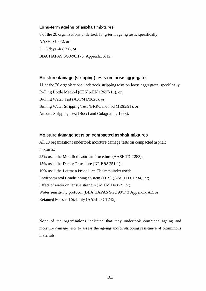
B.2

Long-term ageing of asphalt mixtures 8 of the 20 organisations undertook long-term ageing tests, specifically;

AASHTO PP2, or;

2 – 8 days @ 85°C, or;

BBA HAPAS SG3/98/173, Appendix A12.

Moisture damage (stripping) tests on loose aggregates 11 of the 20 organisations undertook stripping tests on loose aggregates, specifically;

Rolling Bottle Method (CEN prEN 12697-11), or;

Boiling Water Test (ASTM D3625), or;

Boiling Water Stripping Test (BRRC method ME65/91), or;

Ancona Stripping Test (Bocci and Colagrande, 1993).

Moisture damage tests on compacted asphalt mixtures All 20 organisations undertook moisture damage tests on compacted asphalt

mixtures;

25% used the Modified Lottman Procedure (AASHTO T283);

15% used the Duriez Procedure (NF P 98 251-1);

10% used the Lottman Procedure. The remainder used;

Environmental Conditioning System (ECS) (AASHTO TP34), or;

Effect of water on tensile strength (ASTM D4867), or;

Water sensitivity protocol (BBA HAPAS SG3/98/173 Appendix A2, or;

Retained Marshall Stability (AASHTO T245).

None of the organisations indicated that they undertook combined ageing and

moisture damage tests to assess the ageing and/or stripping resistance of bituminous

materials.

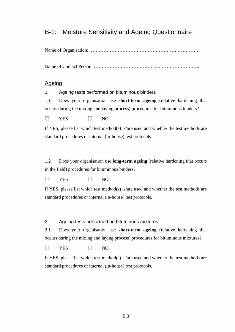
B.3

B-1: Moisture Sensitivity and Ageing Questionnaire

Name of Organisation: ……………………………………………………………

Name of Contact Person: ………………………………………………………….

Ageing 1 Ageing tests performed on bituminous binders

1.1 Does your organisation use short-term ageing (relative hardening that

occurs during the mixing and laying process) procedures for bituminous binders?

YES NO

If YES, please list which test method(s) is/are used and whether the test methods are

standard procedures or internal (in-house) test protocols.

1.2 Does your organisation use long-term ageing (relative hardening that occurs

in the field) procedures for bituminous binders?

YES NO

If YES, please list which test method(s) is/are used and whether the test methods are

standard procedures or internal (in-house) test protocols.

2 Ageing tests performed on bituminous mixtures

2.1 Does your organisation use short-term ageing (relative hardening that

occurs during the mixing and laying process) procedures for bituminous mixtures?

YES NO

If YES, please list which test method(s) is/are used and whether the test methods are

standard procedures or internal (in-house) test protocols.

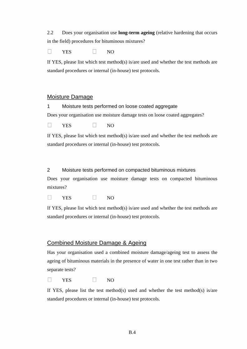
B.4

2.2 Does your organisation use long-term ageing (relative hardening that occurs

in the field) procedures for bituminous mixtures?

YES NO

If YES, please list which test method(s) is/are used and whether the test methods are

standard procedures or internal (in-house) test protocols.

Moisture Damage

1 Moisture tests performed on loose coated aggregate

Does your organisation use moisture damage tests on loose coated aggregates?

YES NO

If YES, please list which test method(s) is/are used and whether the test methods are

standard procedures or internal (in-house) test protocols.

2 Moisture tests performed on compacted bituminous mixtures

Does your organisation use moisture damage tests on compacted bituminous

mixtures?

YES NO

If YES, please list which test method(s) is/are used and whether the test methods are

standard procedures or internal (in-house) test protocols.

Combined Moisture Damage & Ageing Has your organisation used a combined moisture damage/ageing test to assess the

ageing of bituminous materials in the presence of water in one test rather than in two

separate tests?

YES NO

If YES, please list the test method(s) used and whether the test method(s) is/are

standard procedures or internal (in-house) test protocols.

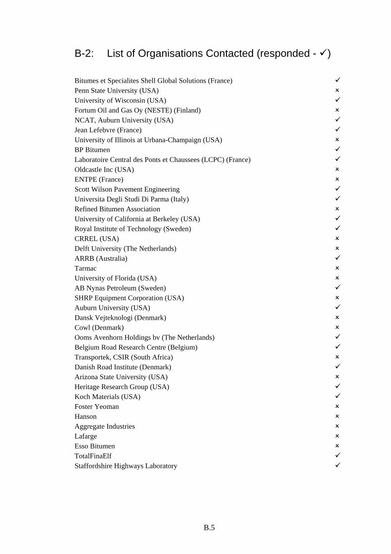
B.5

B-2: List of Organisations Contacted (responded - ) Bitumes et Specialites Shell Global Solutions (France) Penn State University (USA) University of Wisconsin (USA) Fortum Oil and Gas Oy (NESTE) (Finland) NCAT, Auburn University (USA) Jean Lefebvre (France) University of Illinois at Urbana-Champaign (USA) BP Bitumen Laboratoire Central des Ponts et Chaussees (LCPC) (France) Oldcastle Inc (USA) ENTPE (France) Scott Wilson Pavement Engineering Universita Degli Studi Di Parma (Italy) Refined Bitumen Association University of California at Berkeley (USA) Royal Institute of Technology (Sweden) CRREL (USA) Delft University (The Netherlands) ARRB (Australia) Tarmac University of Florida (USA) AB Nynas Petroleum (Sweden) SHRP Equipment Corporation (USA) Auburn University (USA) Dansk Vejteknologi (Denmark) Cowl (Denmark) Ooms Avenhorn Holdings bv (The Netherlands) Belgium Road Research Centre (Belgium) Transportek, CSIR (South Africa) Danish Road Institute (Denmark) Arizona State University (USA) Heritage Research Group (USA) Koch Materials (USA) Foster Yeoman Hanson Aggregate Industries Lafarge Esso Bitumen TotalFinaElf Staffordshire Highways Laboratory

C.1

Appendix C. Binder Characterisation Tests

C.1 Introduction

This chapter describes the binder characterisation tests performed on the four binders

used in the research. A series of tests were performed on the unconditioned binders

as well as after short term (RTFOT) and long term (HiPAT) ageing.

C.1.1 Binders

Three 15 penetration grade binders (referred to as 15B, 15D and 15E) and a 50

penetration grade binder (referred to as 50C) were tested.

C.1.2 Ageing Processes

The above binders were subjected to short term (RTFOT) and long term (HiPAT)

ageing. Details of these two procedures can be found respectively, in references [EN

12607-1, 1999; BBA/HAPAS SG4, 2001].

C.2 Penetration Test

The penetration test [BS 2000-49, 2000] was performed at 25oC and 40oC for this

project. Table C.1 shows the individual results.

C.3 Softening Point Test

The Softening Point test was performed as described in references [BS 2000-58,

2000]. The results are presented in Table C.2.

C.2

Table C.1 – Penetration test results

Binder 15B 15D 15E 50C

Temp. (oC) 25 40 25 40 25 50 25 40

Unaged 15 62 14 39 15 70 53 263

RTFOT 11 36 8 30 13 41 35 146

HiPAT 6 20 4 16 7 25 17 69

Table C.2 – Softening point test results

Binder 15B 15D 15E 50C

Unaged 68.0 73.0 62.0 49.0

RTFOT 75.4 79.0 67.0 55.0

HiPAT 96.0 98.0 78.0 65.0

C.4 Rotational Viscosity Test

This test was performed to investigate the viscosity of binder as described in

reference [BS 2000-505, 2003]. The test was performed in a temperature range of

60oC to 135oC. The results are presented in Table C.3.

C.5 Bitumen Test Data Chart

The results from the penetration, softening point and viscosity tests for 15B, 15D,

15E and 50C are presented using the bitumen test data chart (BTDC) in Figures C.1

to C.4.

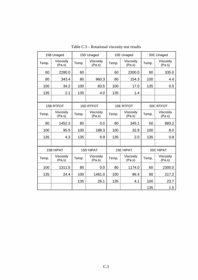
C.3

Table C.3 – Rotational viscosity test results

15B Unaged 15D Unaged 15E Unaged 50C Unaged

Temp. Viscosity (Pa.s) Temp. Viscosity

(Pa.s) Temp. Viscosity (Pa.s) Temp. Viscosity

(Pa.s)

60 2280.0 60 60 2300.0 60 335.0

80 343.4 80 960.3 80 154.3 100 4.4

100 34.2 100 83.5 100 17.0 135 0.5

135 2.1 135 4.0 135 1.4

15B RTFOT 15D RTFOT 15E RTFOT 50C RTFOT

Temp. Viscosity (Pa.s) Temp. Viscosity

(Pa.s) Temp. Viscosity (Pa.s) Temp. Viscosity

(Pa.s)

80 1452.3 80 0.0 80 345.1 60 883.2

100 95.5 100 188.3 100 32.9 100 8.0

135 4.3 135 6.9 135 2.0 135 0.8

15B HiPAT 15D HiPAT 15E HiPAT 50C HiPAT

Temp. Viscosity (Pa.s) Temp. Viscosity

(Pa.s) Temp. Viscosity (Pa.s) Temp. Viscosity

(Pa.s)

100 1311.5 80 0.0 80 1174.0 60 2300.0

135 24.4 100 1481.0 100 86.4 80 217.2

135 26.1 135 4.1 100 23.7

135 1.5

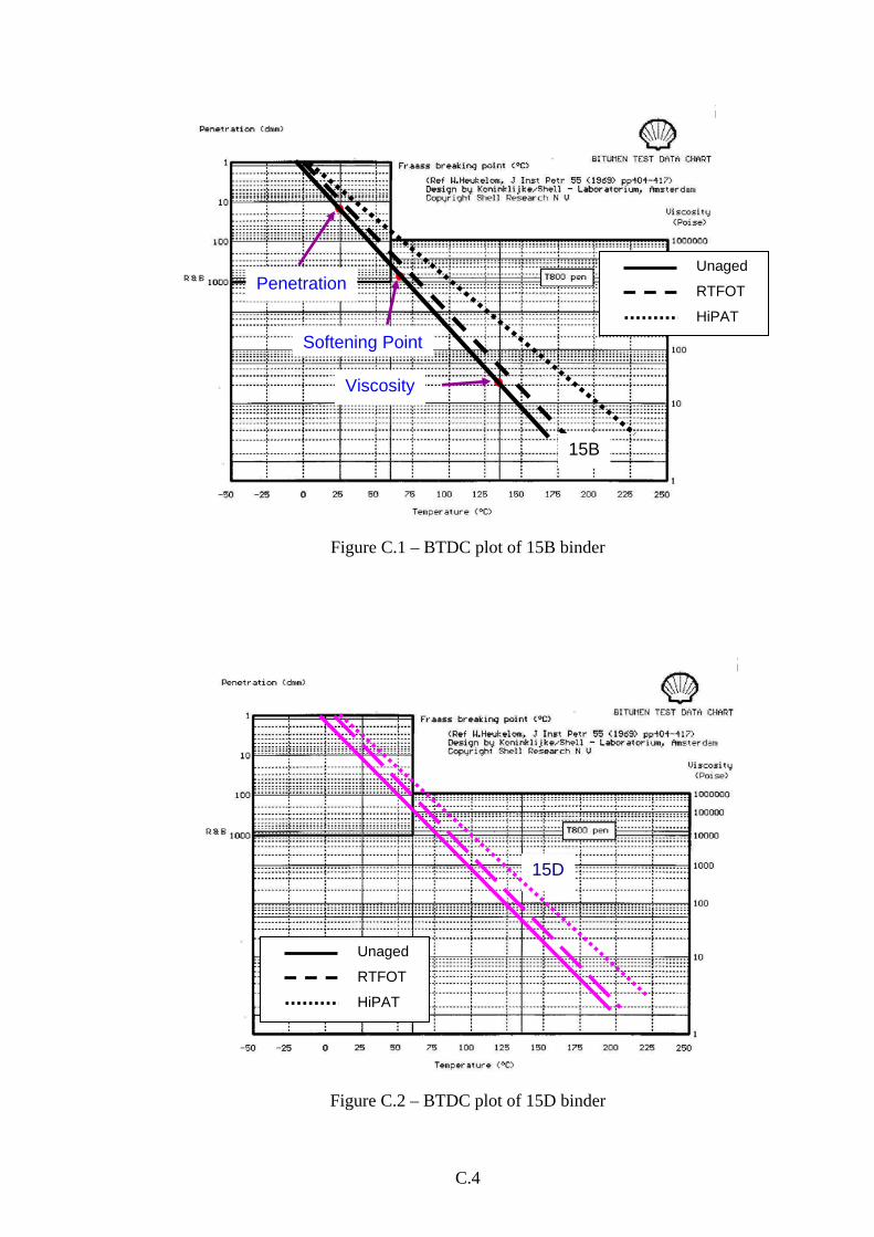
C.4

Figure C.1 – BTDC plot of 15B binder

Figure C.2 – BTDC plot of 15D binder

Penetration

Softening Point

Viscosity

15B

Unaged

RTFOT

HiPAT

15D

Unaged

RTFOT

HiPAT

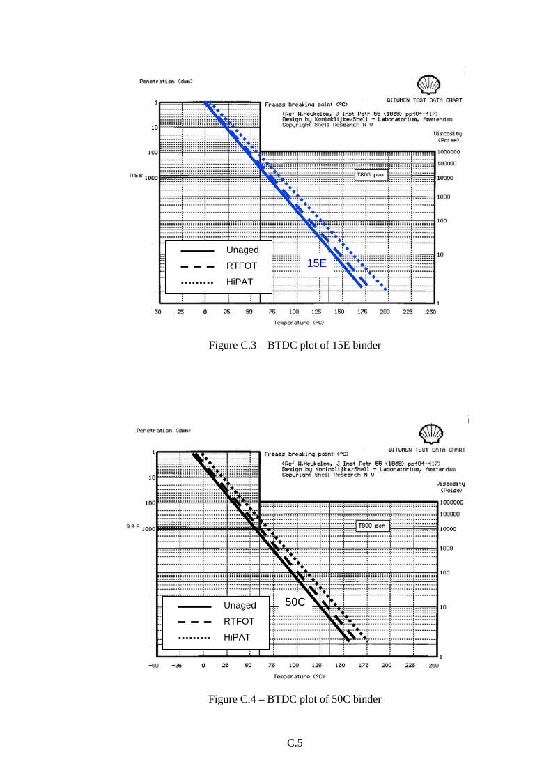
C.5

Figure C.3 – BTDC plot of 15E binder

Figure C.4 – BTDC plot of 50C binder

15E Unaged

RTFOT

HiPAT

50C Unaged

RTFOT

HiPAT

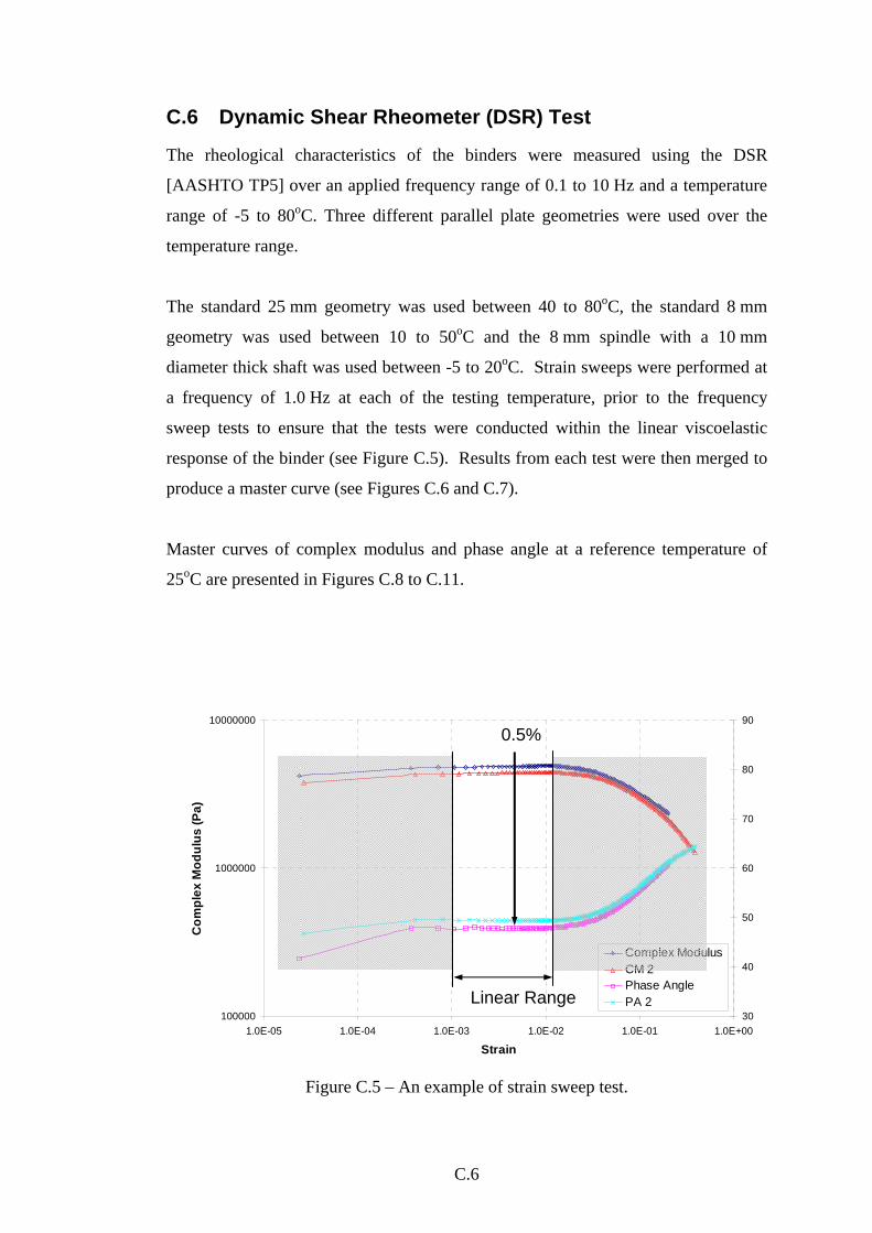
C.6

C.6 Dynamic Shear Rheometer (DSR) Test

The rheological characteristics of the binders were measured using the DSR

[AASHTO TP5] over an applied frequency range of 0.1 to 10 Hz and a temperature

range of -5 to 80oC. Three different parallel plate geometries were used over the

temperature range.

The standard 25 mm geometry was used between 40 to 80oC, the standard 8 mm

geometry was used between 10 to 50oC and the 8 mm spindle with a 10 mm

diameter thick shaft was used between -5 to 20oC. Strain sweeps were performed at

a frequency of 1.0 Hz at each of the testing temperature, prior to the frequency

sweep tests to ensure that the tests were conducted within the linear viscoelastic

response of the binder (see Figure C.5). Results from each test were then merged to

produce a master curve (see Figures C.6 and C.7).

Master curves of complex modulus and phase angle at a reference temperature of

25oC are presented in Figures C.8 to C.11.

Figure C.5 – An example of strain sweep test.

100000

1000000

10000000

1.0E-05 1.0E-04 1.0E-03 1.0E-02 1.0E-01 1.0E+00

Strain

Com

plex

Mod

ulus

(Pa)

30

40

50

60

70

80

90

Complex ModulusCM 2Phase AnglePA 2

0.5%

Linear Range

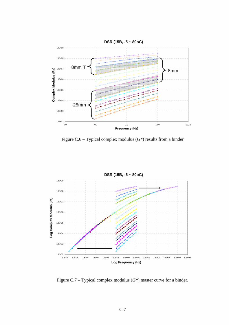
C.7

Figure C.6 – Typical complex modulus (G*) results from a binder

Figure C.7 – Typical complex modulus (G*) master curve for a binder.

DSR (15B, -5 ~ 80oC)

1.E+02

1.E+03

1.E+04

1.E+05

1.E+06

1.E+07

1.E+08

1.E+09

0.0 0.1 1.0 10.0 100.0

Frequency (Hz)

Com

plex

Mod

ulus

(Pa)

25mm

8mm 8mm T

DSR (15B, -5 ~ 80oC)

1.E+02

1.E+03

1.E+04

1.E+05

1.E+06

1.E+07

1.E+08

1.E+09

1.E-06 1.E-05 1.E-04 1.E-03 1.E-02 1.E-01 1.E+00 1.E+01 1.E+02 1.E+03 1.E+04 1.E+05 1.E+06

Log Frequency (Hz)

Log

Com

plex

Mod

ulus

(Pa)

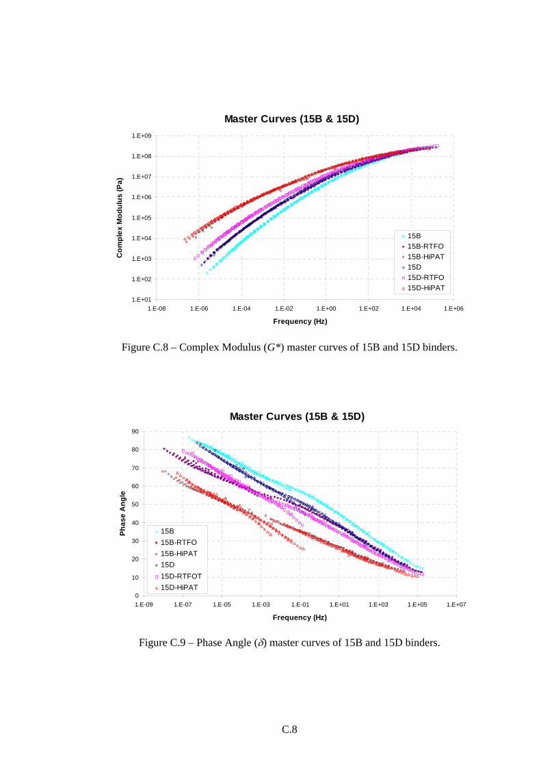
C.8

Figure C.8 – Complex Modulus (G*) master curves of 15B and 15D binders.

Figure C.9 – Phase Angle (δ) master curves of 15B and 15D binders.

Master Curves (15B & 15D)

1.E+01

1.E+02

1.E+03

1.E+04

1.E+05

1.E+06

1.E+07

1.E+08

1.E+09

1.E-08 1.E-06 1.E-04 1.E-02 1.E+00 1.E+02 1.E+04 1.E+06

Frequency (Hz)

Com

plex

Mod

ulus

(Pa)

15B15B-RTFO15B-HiPAT15D15D-RTFO15D-HiPAT

Master Curves (15B & 15D)

0

10

20

30

40

50

60

70

80

90

1.E-09 1.E-07 1.E-05 1.E-03 1.E-01 1.E+01 1.E+03 1.E+05 1.E+07

Frequency (Hz)

Phas

e A

ngle

15B15B-RTFO15B-HiPAT15D15D-RTFOT15D-HiPAT

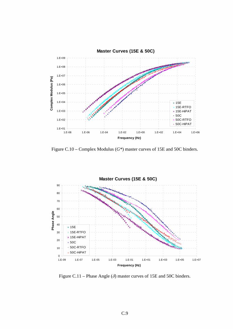
C.9

Figure C.10 – Complex Modulus (G*) master curves of 15E and 50C binders.

Figure C.11 – Phase Angle (δ) master curves of 15E and 50C binders.

Master Curves (15E & 50C)

1.E+01

1.E+02

1.E+03

1.E+04

1.E+05

1.E+06

1.E+07

1.E+08

1.E+09

1.E-08 1.E-06 1.E-04 1.E-02 1.E+00 1.E+02 1.E+04 1.E+06

Frequency (Hz)

Com

plex

Mod

ulus

(Pa)

15E15E-RTFO15E-HiPAT50C50C-RTFO50C-HiPAT

Master Curves (15E & 50C)

0

10

20

30

40

50

60

70

80

90

1.E-09 1.E-07 1.E-05 1.E-03 1.E-01 1.E+01 1.E+03 1.E+05 1.E+07

Frequency (Hz)

Phas

e A

ngle

15E15E-RTFO15E-HiPAT50C50C-RTFO50C-HiPAT

C.10

C.6.1 Review of Dynamic Shear Rheometer Results

From Figures C.8 to C.11, binders 15B and 15E (unaged) have similar G* values but

15E is more viscous (i.e. higher δ), particularly at low/intermediate frequencies.

Among the 15 Pen grade binders, 15B showed the largest change in G* values and

phase angle (δ) due to ageing, while 15E showed the least. 15D showed the highest

G* value and lowest phase angle (δ) among the unaged 15 Pen binders, but showed

almost identical characteristics after long-term ageing.

Long-term aged 50C binder showed similar G* values to those of the 15 Pen unaged

binders (particularly 15B and 15E), while the phase angles (δ) showed similar values

to those of 15B and 15D.

D.1

Draft for Development

Method for the Assessment of Durability of Compacted

Asphalt Mixtures using the Saturated Ageing Tensile Stiffness

(SATS) Test

1. Scope This Draft for Development specifies a test method to assess the sensitivity of

asphalt pavement materials to a combined ageing moisture sensitivity

procedure, by measuring stiffness before and after the test.

The test method is intended to simulate the effect of ageing and moisture on

asphalt pavement materials in service. It is suitable for coated macadam base

and binder course mixtures with a nominal air void content of 8% and a

nominal binder content of 4%. The test may not be suitable for mixtures of

high binder content or manufactured with binders of penetration higher than

50.

2. Normative References This Draft for Development incorporates by dated or undated reference,

provisions from other publications. These normative references are cited at the

appropriate places in the text, and the publications are listed hereafter. For

dated references, subsequent amendments to or revisions of any of these

publications apply to this Draft for Development only when incorporated in it

by amendment or revision. For undated references the latest edition of the

publication referred to applies (including amendments).

British Standard Draft for Development DD 213: 1993 Method for

determination of the indirect tensile stiffness modulus of bituminous mixtures.

D.2

British Standard BS EN 12697-5: 2002 Bituminous mixtures – Test Methods

for hot mix asphalt Part 5: Determination of the maximum density.

British Standard BS 598-100: 1987 (1996) Sampling and examination of

bituminous mixtures for roads and other paved areas Part 100: Methods for

sampling for analysis.

British Standard BS 598-104: 1989 Sampling and examination of bituminous

mixtures for roads and other paved areas Part 104: Method of test for the

determination of density and compaction.

British Standard BS 6100 (1984 on) Glossary of building and civil engineering

terms.

AASHTO Designation PP1, Edition 1A: 1993 Standard practice for

accelerated ageing of asphalt binder using a pressurized ageing vessel (PAV).

3. Terms and Definitions For the purposes of this Draft for Development the following terms and

definitions given in BS 6100 apply, together with the following.

3.1 Maximum Density

Mass per unit volume, without air voids, of a bituminous mixture at known test

temperature.

3.2 Dry Bulk Density

Mass per unit volume, including the air voids, of a specimen at known test

temperature.

3.3 Saturation Before Conditioning

D.3

The saturation of the mixture, determined as the calculated percentage of air

voids filled with water after partial saturation, prior to conditioning as

described in this Draft for Development.

3.4 Unconditioned Stiffness

The stiffness modulus of the mixture as determined in accordance with BS DD

213: 1993, prior to conditioning as described in this Draft for Development.

3.5 Conditioned Stiffness

The stiffness modulus of the mixtures as determined in accordance in

accordance with BS DD 213: 1993, after conditioning as described in this Draft

for Development.

3.6 Stiffness Ratio

The ratio of the conditioned stiffness to the unconditioned stiffness.

3.7 Saturation After Conditioning

The saturation of the mixture, determined as the calculated percentage of air

voids filled with water after conditioning as described in this Draft for

Development.

4. Principle of Test Nominally identical test specimens are subjected to moisture saturation by

using a vacuum system and then transferred into a pressurised ageing vessel

partially filled with water, where they are subjected to a conditioning procedure

at 85°C temperature and 2.1 MPa pressure for 65 hours. The stiffness of

individual specimens after the conditioning procedure, expressed as a

percentage of the stiffness before the conditioning procedure, is plotted against

their percentage saturation to determine the sensitivity of the material to ageing

and moisture. The whole process is referred to as the saturated ageing tensile

stiffness (SATS) test.

D.4

5. Materials

5.1 De-aired (distilled) water, freshly de-aired and cooled

5.2 Self-adhesive aluminium foil: Capable of adhering to and covering the

specimen with an impervious coating.

5.3 Absorbent paper towelling.

6. Apparatus

6.1 Vacuum desiccator and vacuum pump, including manometer or calibrated

vacuum gauge as described in BS EN 12697-5.

6.2 Balance with sufficient capacity and accurate to at least 1g.

6.3 Pressure Vessel as described in AASHTO PP1, and of sufficient capacity to

accommodate five test specimens for a full test. Dimensions of a suitable

vessel are shown in Figure 1.

6.4 Nottingham Asphalt Tester (NAT) capable of performing the Indirect Tensile

Stiffness Modulus (ITSM) test on compacted bituminous mixture specimens in

accordance with BS DD213.

6.5 Specimen tray, to accommodate five test specimens for a full test. Dimensions

of a suitable tray are shown in Figure 2.

7. Sample Preparation

Test specimens shall be cores of 100 + 0, -5 mm diameter and 60 ± 5 mm thickness.

The standard procedure involves specimens cored from a slab manufactured using a

laboratory roller compactor. Five nominally identical specimens are required for the

full test. Specimens for test may also be cores from an in-service pavement in

accordance with BS 598-100.

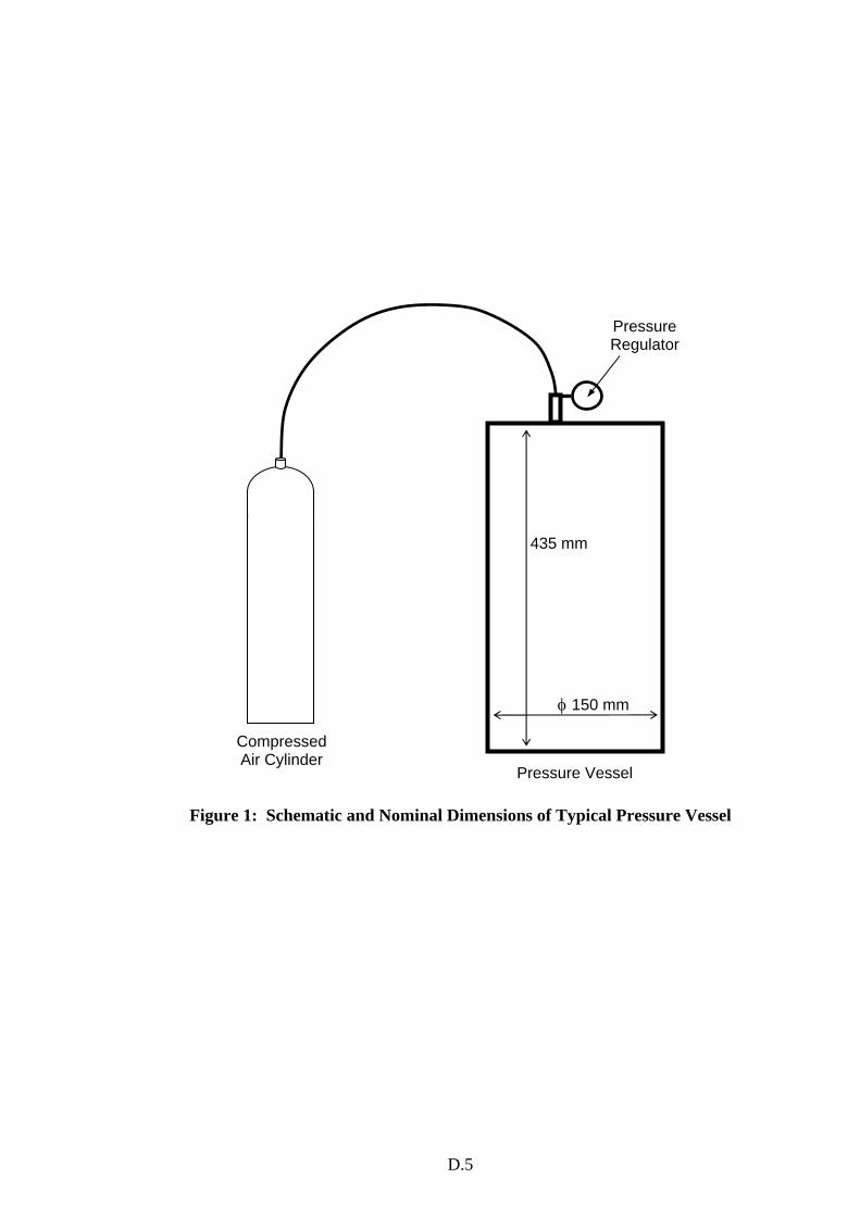
D.5

Figure 1: Schematic and Nominal Dimensions of Typical Pressure Vessel

Pressure Vessel

φ 150 mm

435 mm

Pressure Regulator

Compressed Air Cylinder

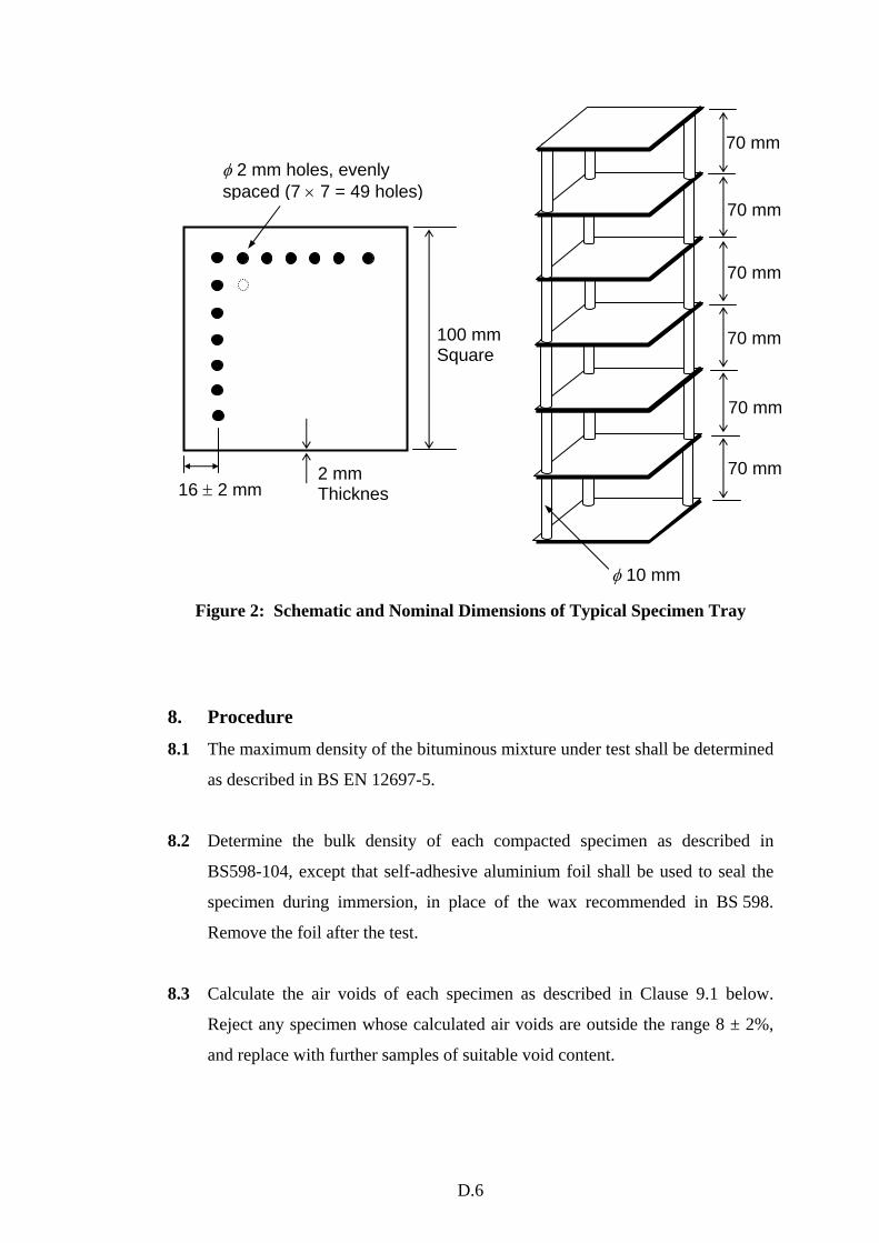
D.6

Figure 2: Schematic and Nominal Dimensions of Typical Specimen Tray

8. Procedure

8.1 The maximum density of the bituminous mixture under test shall be determined

as described in BS EN 12697-5.

8.2 Determine the bulk density of each compacted specimen as described in

BS598-104, except that self-adhesive aluminium foil shall be used to seal the

specimen during immersion, in place of the wax recommended in BS 598.

Remove the foil after the test.

8.3 Calculate the air voids of each specimen as described in Clause 9.1 below.

Reject any specimen whose calculated air voids are outside the range 8 ± 2%,

and replace with further samples of suitable void content.

φ 2 mm holes, evenly spaced (7 × 7 = 49 holes)

100 mm Square

2 mm Thicknes16 ± 2 mm

70 mm

70 mm

φ 10 mm

70 mm

70 mm

70 mm

70 mm

D.7

8.4 Determine the unconditioned (initial) stiffness modulus at 20 ± 5°C in the

NAT. Designate this as ITSMU.

8.5 Determine the dry mass of each specimen using the balance and designate this

as Md.

8.6 Place the specimens in the vacuum desiccator, cover them with distilled water

at 20 ± 1°C, seal the apparatus, and apply a partial vacuum pressure of 68 ±

3 kPa for 30 minutes.

8.7 Remove each specimen from the vacuum desiccator, remove any water on its

surface using the absorbent paper towelling and determine its wet mass.

Designate this as Mw. Determine the percent saturation (S) as described in

Clause 9.2 below. Reject any specimens whose calculated saturation is ≥ 80%.

8.8 Partly fill the pressure vessel with water. The water level should be between

the 4th and 5th specimen, as shown in the schematic in Figure 3. Use freshly

distilled water only (do not re-use). The vessel and water should be

controlled to the target temperature at least 2 hours before the conditioning

procedure commences.

8.9 Place the specimens into the vessel, using the specimen tray, and perform the

conditioning procedure, as described in AASHTO PP1, at 2.1 ± 0.1 MPa

pressure and 85 ± 1°C for 65 ± 1h.

8.10 After the test period of 65h has elapsed, turn off the heater and release the

pressure from the vessel slowly. Adjust the pressure release mechanism so

that the pressure returns to atmospheric pressure over a period of 20 to

30 minutes. Do not open the cover at this stage.

8.11 When the pressure vessel display temperature has reduced to 70°C (this may

take up to 3 hours) open the cover and extract all the specimens, on the tray,

from the vessel.

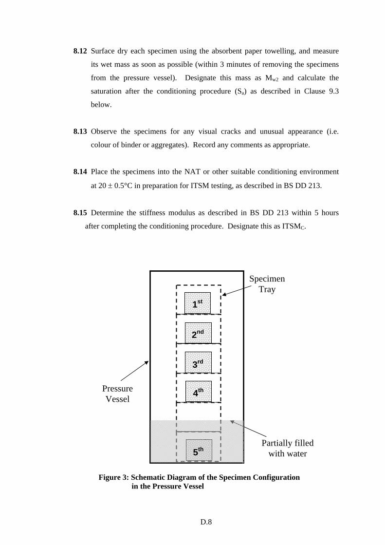
D.8

8.12 Surface dry each specimen using the absorbent paper towelling, and measure

its wet mass as soon as possible (within 3 minutes of removing the specimens

from the pressure vessel). Designate this mass as Mw2 and calculate the

saturation after the conditioning procedure (Sa) as described in Clause 9.3

below.

8.13 Observe the specimens for any visual cracks and unusual appearance (i.e.

colour of binder or aggregates). Record any comments as appropriate.

8.14 Place the specimens into the NAT or other suitable conditioning environment

at 20 ± 0.5°C in preparation for ITSM testing, as described in BS DD 213.

8.15 Determine the stiffness modulus as described in BS DD 213 within 5 hours

after completing the conditioning procedure. Designate this as ITSMC.

Figure 3: Schematic Diagram of the Specimen Configuration in the Pressure Vessel

Specimen Tray

Partially filled with water

1st

2nd

3rd

4th

5th

Pressure Vessel

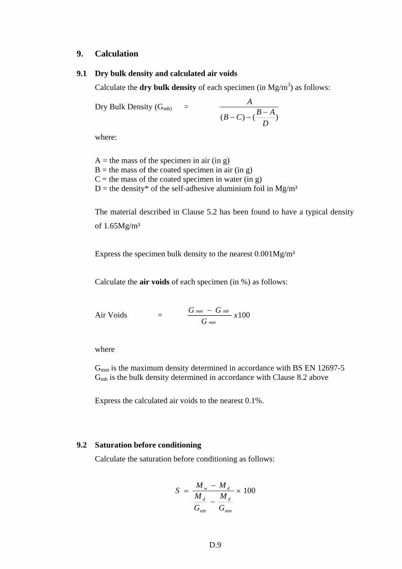
D.9

9. Calculation

9.1 Dry bulk density and calculated air voids

Calculate the dry bulk density of each specimen (in Mg/m3) as follows:

Dry Bulk Density (Gmb) = )()(

DABCB

A−

−−

where:

A = the mass of the specimen in air (in g) B = the mass of the coated specimen in air (in g) C = the mass of the coated specimen in water (in g) D = the density* of the self-adhesive aluminium foil in Mg/m³

The material described in Clause 5.2 has been found to have a typical density

of 1.65Mg/m³

Express the specimen bulk density to the nearest 0.001Mg/m³

Calculate the air voids of each specimen (in %) as follows:

Air Voids = 100xG

GGmm

mbmm −

where Gmm is the maximum density determined in accordance with BS EN 12697-5 Gmb is the bulk density determined in accordance with Clause 8.2 above

Express the calculated air voids to the nearest 0.1%.

9.2 Saturation before conditioning

Calculate the saturation before conditioning as follows:

100×−

−=

mm

d

mb

d

dw

GM

GM

MMS

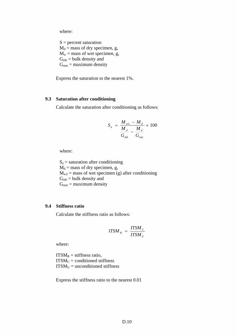
D.10

where: S = percent saturation Md = mass of dry specimen, g, Mw = mass of wet specimen, g, Gmb = bulk density and Gmm = maximum density

Express the saturation to the nearest 1%.

9.3 Saturation after conditioning

Calculate the saturation after conditioning as follows:

1002 ×−

−=

mm

d

mb

d

dwa

GM

GM

MMS

where: Sa = saturation after conditioning Md = mass of dry specimen, g, Mw2 = mass of wet specimen (g) after conditioning Gmb = bulk density and Gmm = maximum density

9.4 Stiffness ratio

Calculate the stiffness ratio as follows:

U

CR ITSM

ITSMITSM =

where: ITSMR = stiffness ratio, ITSMC = conditioned stiffness ITSMU = unconditioned stiffness

Express the stiffness ratio to the nearest 0.01

D.11

10. Precision

The precision for this test method has not been established.

11. Report

With reference to this Draft for Development, the test report shall include the

following information:

a) Reference to this test method and test conditions

b) Maximum density of the mixture tested, to the nearest 0.001 Mg/m³

c) For each specimen tested, report

- Bulk density (Gmb), to the nearest 0.001 Mg/m³

- Percent air voids (Vv), to the nearest 0.1%

- Percent saturation (S) before conditioning, to the nearest 1%

- Percent saturation after conditioning, (Sa), to the nearest 1%

- Unconditioned stiffness (ITSMU) before conditioning, to the nearest 100 MPa

- Conditioned stiffness (ITSMC) after conditioning, to the nearest 100 MPa

- Stiffness ratio (ITSMR), to the nearest 0.01

- Any cracks or other damage.

d) For the mixture tested, the stiffness ratio of the individual specimens

tested shall be plotted against the corresponding saturation value after

saturation. A graphical representation of a typical set of data is shown in

Figure 4.

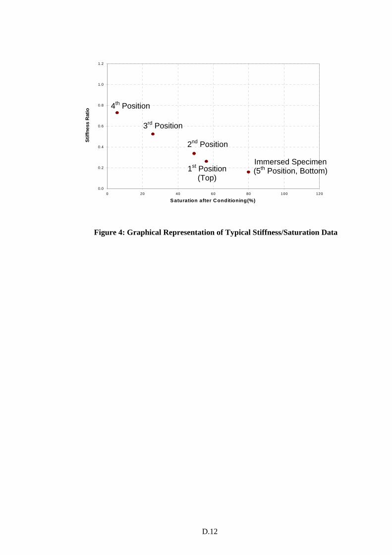
D.12

Figure 4: Graphical Representation of Typical Stiffness/Saturation Data

0.0

0.2

0.4

0.6

0.8

1.0

1.2

0 20 40 60 80 100 120

Saturation after Conditioning(%)

Stiff

ness

Rat

io

Immersed Specimen (5th Position, Bottom)

4th Position

1st Position (Top)

3rd Position

2nd Position

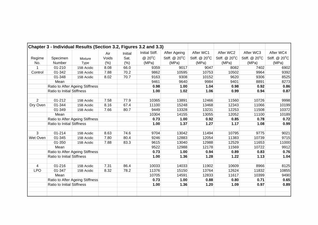
Chapter 3 - Individual Results (Section 3.2, Figures 3.2 and 3.3)

RegimeNo.

SpecimenNumber

MixtureType

AirVoids(%)

InitialSat.(%)

Initial Stiff.@ 20oC (MPa)

After AgeingStiff. @ 20oC

(MPa)

After WC1Stiff. @ 20oC

(MPa)

After WC2Stiff. @ 20oC

(MPa)

After WC3Stiff. @ 20oC

(MPa)

After WC4Stiff. @ 20oC

(MPa)1 01-210 15B Acidic 8.08 66.0 9359 9017 9047 8082 7402 6902

Control 01-342 15B Acidic 7.88 70.2 9862 10595 10753 10502 9964 939201-348 15B Acidic 8.02 70.7 9163 9308 10152 9620 9306 8525Mean 9461 9640 9984 9401 8891 8273

Ratio to After Ageing Stiffness 0.98 1.00 1.04 0.98 0.92 0.86Ratio to Initial Stiffness 1.00 1.02 1.06 0.99 0.94 0.87

2 01-212 15B Acidic 7.58 77.9 10365 13891 12466 11560 10726 9998Dry Oven 01-344 15B Acidic 8.16 67.4 11100 15248 13468 12343 11066 10199

01-349 15B Acidic 7.66 80.7 9449 13328 13231 12253 11508 10372Mean 10304 14155 13055 12052 11100 10189

Ratio to After Ageing Stiffness 0.73 1.00 0.92 0.85 0.78 0.72Ratio to Initial Stiffness 1.00 1.37 1.27 1.17 1.08 0.99

3 01-214 15B Acidic 8.63 74.6 9704 13042 11494 10795 9775 9021Wet Oven 01-345 15B Acidic 7.80 80.4 9246 12883 12054 11383 10739 9715

01-350 15B Acidic 7.88 83.3 9615 13040 12988 12529 11653 11000Mean 9522 12988 12178 11569 10722 9912

Ratio to After Ageing Stiffness 0.73 1.00 0.94 0.89 0.83 0.76Ratio to Initial Stiffness 1.00 1.36 1.28 1.22 1.13 1.04

4 01-216 15B Acidic 7.31 86.4 10033 14033 11902 10609 8966 8125LPO 01-347 15B Acidic 8.32 78.2 11376 15150 13764 12624 11832 10855

Mean 10705 14591 12833 11617 10399 9490Ratio to After Ageing Stiffness 0.73 1.00 0.88 0.80 0.71 0.65Ratio to Initial Stiffness 1.00 1.36 1.20 1.09 0.97 0.89

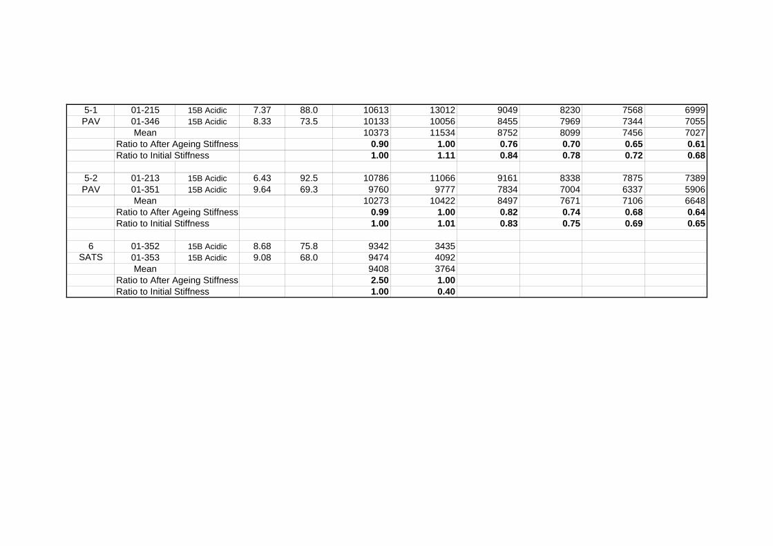
5-1 01-215 15B Acidic 7.37 88.0 10613 13012 9049 8230 7568 6999PAV 01-346 15B Acidic 8.33 73.5 10133 10056 8455 7969 7344 7055

Mean 10373 11534 8752 8099 7456 7027Ratio to After Ageing Stiffness 0.90 1.00 0.76 0.70 0.65 0.61Ratio to Initial Stiffness 1.00 1.11 0.84 0.78 0.72 0.68

5-2 01-213 15B Acidic 6.43 92.5 10786 11066 9161 8338 7875 7389PAV 01-351 15B Acidic 9.64 69.3 9760 9777 7834 7004 6337 5906

Mean 10273 10422 8497 7671 7106 6648Ratio to After Ageing Stiffness 0.99 1.00 0.82 0.74 0.68 0.64Ratio to Initial Stiffness 1.00 1.01 0.83 0.75 0.69 0.65

6 01-352 15B Acidic 8.68 75.8 9342 3435SATS 01-353 15B Acidic 9.08 68.0 9474 4092

Mean 9408 3764Ratio to After Ageing Stiffness 2.50 1.00Ratio to Initial Stiffness 1.00 0.40

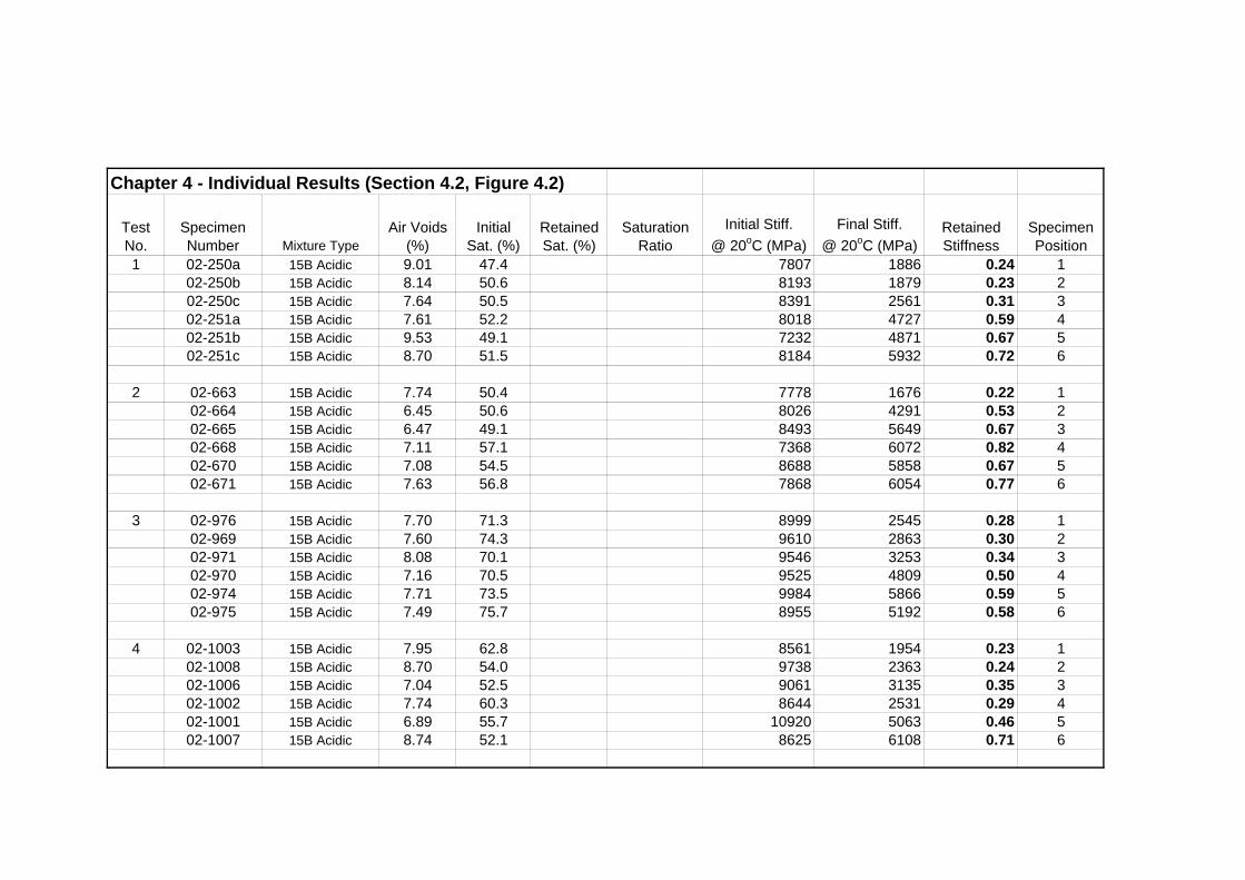
Chapter 4 - Individual Results (Section 4.2, Figure 4.2)

TestNo.

SpecimenNumber Mixture Type

Air Voids(%)

InitialSat. (%)

RetainedSat. (%)

Saturation Ratio

Initial Stiff.@ 20oC (MPa)

Final Stiff.@ 20oC (MPa)

RetainedStiffness

SpecimenPosition

1 02-250a 15B Acidic 9.01 47.4 7807 1886 0.24 102-250b 15B Acidic 8.14 50.6 8193 1879 0.23 202-250c 15B Acidic 7.64 50.5 8391 2561 0.31 302-251a 15B Acidic 7.61 52.2 8018 4727 0.59 402-251b 15B Acidic 9.53 49.1 7232 4871 0.67 502-251c 15B Acidic 8.70 51.5 8184 5932 0.72 6

2 02-663 15B Acidic 7.74 50.4 7778 1676 0.22 102-664 15B Acidic 6.45 50.6 8026 4291 0.53 202-665 15B Acidic 6.47 49.1 8493 5649 0.67 302-668 15B Acidic 7.11 57.1 7368 6072 0.82 402-670 15B Acidic 7.08 54.5 8688 5858 0.67 502-671 15B Acidic 7.63 56.8 7868 6054 0.77 6

3 02-976 15B Acidic 7.70 71.3 8999 2545 0.28 102-969 15B Acidic 7.60 74.3 9610 2863 0.30 202-971 15B Acidic 8.08 70.1 9546 3253 0.34 302-970 15B Acidic 7.16 70.5 9525 4809 0.50 402-974 15B Acidic 7.71 73.5 9984 5866 0.59 502-975 15B Acidic 7.49 75.7 8955 5192 0.58 6

4 02-1003 15B Acidic 7.95 62.8 8561 1954 0.23 102-1008 15B Acidic 8.70 54.0 9738 2363 0.24 202-1006 15B Acidic 7.04 52.5 9061 3135 0.35 302-1002 15B Acidic 7.74 60.3 8644 2531 0.29 402-1001 15B Acidic 6.89 55.7 10920 5063 0.46 502-1007 15B Acidic 8.74 52.1 8625 6108 0.71 6

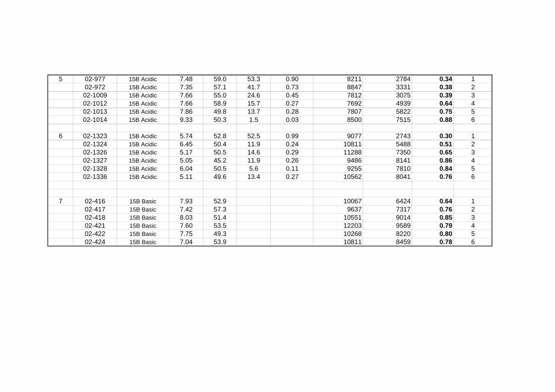
5 02-977 15B Acidic 7.48 59.0 53.3 0.90 8211 2784 0.34 102-972 15B Acidic 7.35 57.1 41.7 0.73 8847 3331 0.38 202-1009 15B Acidic 7.66 55.0 24.6 0.45 7812 3075 0.39 302-1012 15B Acidic 7.66 58.9 15.7 0.27 7692 4939 0.64 402-1013 15B Acidic 7.86 49.8 13.7 0.28 7807 5822 0.75 502-1014 15B Acidic 9.33 50.3 1.5 0.03 8500 7515 0.88 6

6 02-1323 15B Acidic 5.74 52.8 52.5 0.99 9077 2743 0.30 102-1324 15B Acidic 6.45 50.4 11.9 0.24 10811 5488 0.51 202-1326 15B Acidic 5.17 50.5 14.6 0.29 11288 7350 0.65 302-1327 15B Acidic 5.05 45.2 11.9 0.26 9486 8141 0.86 402-1328 15B Acidic 6.04 50.5 5.6 0.11 9255 7810 0.84 502-1336 15B Acidic 5.11 49.6 13.4 0.27 10562 8041 0.76 6

7 02-416 15B Basic 7.93 52.9 10067 6424 0.64 102-417 15B Basic 7.42 57.3 9637 7317 0.76 202-418 15B Basic 8.03 51.4 10551 9014 0.85 302-421 15B Basic 7.60 53.5 12203 9589 0.79 402-422 15B Basic 7.75 49.3 10268 8220 0.80 502-424 15B Basic 7.04 53.9 10811 8459 0.78 6

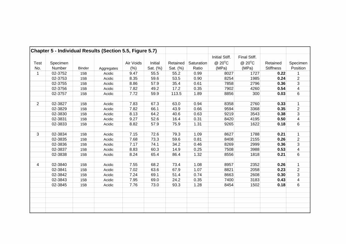
Chapter 5 - Individual Results (Section 5.5, Figure 5.7)

TestNo.

SpecimenNumber Binder Aggregates

Air Voids(%)

InitialSat. (%)

RetainedSat. (%)

SaturationRatio

Initial Stiff.@ 20oC (MPa)

Final Stiff.@ 20oC (MPa)

RetainedStiffness

SpecimenPosition

1 02-3752 15B Acidic 9.47 55.5 55.2 0.99 8027 1727 0.22 102-3753 15B Acidic 8.35 59.6 53.5 0.90 8254 1985 0.24 202-3755 15B Acidic 8.86 57.9 35.4 0.61 7858 2796 0.36 302-3756 15B Acidic 7.82 49.2 17.2 0.35 7902 4260 0.54 402-3757 15B Acidic 7.72 59.9 113.5 1.89 8856 300 0.03 6

2 02-3827 15B Acidic 7.83 67.3 63.0 0.94 8358 2760 0.33 102-3829 15B Acidic 7.82 66.1 43.9 0.66 9594 3368 0.35 202-3830 15B Acidic 8.13 64.2 40.6 0.63 9219 3543 0.38 302-3831 15B Acidic 9.27 52.6 16.4 0.31 8420 4195 0.50 402-3833 15B Acidic 8.82 57.9 75.9 1.31 9265 1622 0.18 6

3 02-3834 15B Acidic 7.15 72.6 79.3 1.09 8627 1788 0.21 102-3835 15B Acidic 7.68 73.3 59.6 0.81 8408 2155 0.26 202-3836 15B Acidic 7.17 74.1 34.2 0.46 8269 2999 0.36 302-3837 15B Acidic 8.83 60.3 14.9 0.25 7508 3988 0.53 402-3838 15B Acidic 8.24 65.4 86.4 1.32 8556 1818 0.21 6

4 02-3840 15B Acidic 7.55 68.2 73.4 1.08 8957 2352 0.26 102-3841 15B Acidic 7.02 63.6 67.9 1.07 8821 2058 0.23 202-3842 15B Acidic 7.24 69.1 51.4 0.74 8663 2608 0.30 302-3843 15B Acidic 7.95 69.0 24.2 0.35 7400 3183 0.43 402-3845 15B Acidic 7.76 73.0 93.3 1.28 8454 1502 0.18 6

5 03-13 15B Basic 8.00 72.0 58.3 0.81 11634 6953 0.60 103-14 15B Basic 7.15 75.5 66.2 0.88 11402 7913 0.69 203-16 15B Basic 8.28 71.9 43.5 0.61 10242 6595 0.64 303-17 15B Basic 9.07 73.5 32.0 0.44 9669 7337 0.76 403-18 15B Basic 8.65 76.3 72.7 0.95 10255 8072 0.79 6

6 03-20 15B Basic 9.59 69.1 51.0 0.74 9400 6488 0.69 103-21 15B Basic 8.56 69.6 39.2 0.56 9454 6735 0.71 203-22 15B Basic 8.54 65.4 35.3 0.54 9825 6670 0.68 303-23 15B Basic 9.12 67.5 31.1 0.46 11249 8452 0.75 403-24 15B Basic 8.65 74.4 74.9 1.01 9799 8001 0.82 6

7 03-25 15B Basic 8.85 79.6 64.2 0.81 9649 6656 0.69 103-27 15B Basic 9.24 72.7 52.5 0.72 10567 7413 0.70 203-28 15B Basic 9.35 61.7 35.3 0.57 9554 6758 0.71 303-29 15B Basic 9.28 70.7 35.5 0.50 9263 6662 0.72 403-30 15B Basic 9.13 73.5 67.5 0.92 8655 5776 0.67 6

8 03-32 15B Basic 9.00 73.1 51.9 0.71 9151 6089 0.67 103-33 15B Basic 7.57 79.8 54.4 0.68 9716 6749 0.69 203-34 15B Basic 9.15 74.3 47.3 0.64 9732 7051 0.72 303-35 15B Basic 7.82 76.9 32.7 0.42 10222 7872 0.77 403-36 15B Basic 9.31 76.0 71.1 0.94 9929 7053 0.71 6

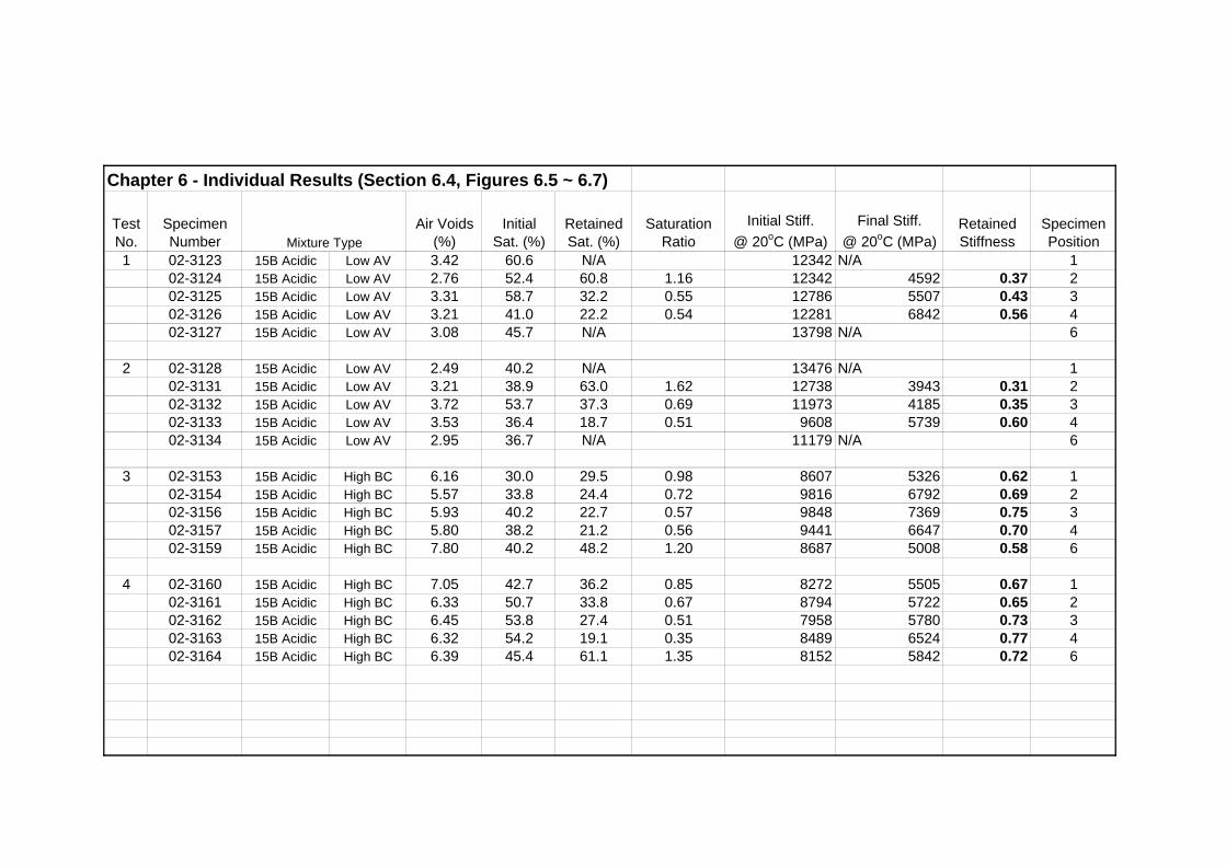
Chapter 6 - Individual Results (Section 6.4, Figures 6.5 ~ 6.7)

TestNo.

SpecimenNumber

Air Voids(%)

InitialSat. (%)

RetainedSat. (%)

Saturation Ratio

Initial Stiff.@ 20oC (MPa)

Final Stiff.@ 20oC (MPa)

RetainedStiffness

SpecimenPosition

1 02-3123 15B Acidic Low AV 3.42 60.6 N/A 12342 N/A 102-3124 15B Acidic Low AV 2.76 52.4 60.8 1.16 12342 4592 0.37 202-3125 15B Acidic Low AV 3.31 58.7 32.2 0.55 12786 5507 0.43 302-3126 15B Acidic Low AV 3.21 41.0 22.2 0.54 12281 6842 0.56 402-3127 15B Acidic Low AV 3.08 45.7 N/A 13798 N/A 6

2 02-3128 15B Acidic Low AV 2.49 40.2 N/A 13476 N/A 102-3131 15B Acidic Low AV 3.21 38.9 63.0 1.62 12738 3943 0.31 202-3132 15B Acidic Low AV 3.72 53.7 37.3 0.69 11973 4185 0.35 302-3133 15B Acidic Low AV 3.53 36.4 18.7 0.51 9608 5739 0.60 402-3134 15B Acidic Low AV 2.95 36.7 N/A 11179 N/A 6

3 02-3153 15B Acidic High BC 6.16 30.0 29.5 0.98 8607 5326 0.62 102-3154 15B Acidic High BC 5.57 33.8 24.4 0.72 9816 6792 0.69 202-3156 15B Acidic High BC 5.93 40.2 22.7 0.57 9848 7369 0.75 302-3157 15B Acidic High BC 5.80 38.2 21.2 0.56 9441 6647 0.70 402-3159 15B Acidic High BC 7.80 40.2 48.2 1.20 8687 5008 0.58 6

4 02-3160 15B Acidic High BC 7.05 42.7 36.2 0.85 8272 5505 0.67 102-3161 15B Acidic High BC 6.33 50.7 33.8 0.67 8794 5722 0.65 202-3162 15B Acidic High BC 6.45 53.8 27.4 0.51 7958 5780 0.73 302-3163 15B Acidic High BC 6.32 54.2 19.1 0.35 8489 6524 0.77 402-3164 15B Acidic High BC 6.39 45.4 61.1 1.35 8152 5842 0.72 6

Mixture Type

5 02-3139 15B Basic Low AV 3.97 41.4 45.9 1.11 14894 7673 0.52 102-3140 15B Basic Low AV 4.41 37.9 29.2 0.77 14205 7649 0.54 202-3141 15B Basic Low AV 3.84 35.2 22.8 0.65 14216 7783 0.55 302-3142 15B Basic Low AV 3.02 29.1 11.9 0.41 12922 8912 0.69 402-3143 15B Basic Low AV 3.90 40.8 89.6 2.20 15351 10462 0.68 6

6 02-3144 15B Basic Low AV 4.07 36.0 40.7 1.13 14540 7628 0.52 102-3145 15B Basic Low AV 3.58 24.2 20.2 0.83 13194 7637 0.58 202-3146 15B Basic Low AV 4.05 56.3 24.9 0.44 14661 7507 0.51 302-3147 15B Basic Low AV 3.82 29.9 14.5 0.48 12828 8656 0.67 402-3148 15B Basic Low AV 4.42 28.6 73.0 2.55 13133 9819 0.75 6

7 02-3168 15B Basic High BC 7.90 55.1 47.7 0.87 10107 5200 0.51 102-3169 15B Basic High BC 6.78 52.5 31.1 0.59 9475 5460 0.58 202-3170 15B Basic High BC 7.66 49.1 27.0 0.55 8461 4851 0.57 302-3173 15B Basic High BC 6.56 46.9 20.9 0.45 8245 5069 0.61 402-3174 15B Basic High BC 7.78 46.9 74.6 1.59 8436 6064 0.72 6

8 02-3175 15B Basic High BC 7.28 53.8 52.0 0.97 8332 4435 0.53 102-3176 15B Basic High BC 7.00 49.3 29.7 0.60 9323 5031 0.54 202-3177 15B Basic High BC 8.69 50.2 28.1 0.56 8819 4446 0.50 302-3178 15B Basic High BC 8.27 53.6 22.1 0.41 9858 6077 0.62 402-3179 15B Basic High BC 7.29 51.4 77.5 1.51 8784 5822 0.66 6

9 02-3231 15E Basic EME2 4.33 63.6 54.4 0.86 9123 4157 0.46 102-3232 15E Basic EME2 4.38 71.2 48.6 0.68 9320 4482 0.48 202-3233 15E Basic EME2 4.02 64.9 40.6 0.62 9197 5008 0.54 302-3234 15E Basic EME2 4.44 69.2 39.4 0.57 9435 4857 0.51 402-3235 15E Basic EME2 4.31 67.8 115.6 1.71 10085 6385 0.63 6

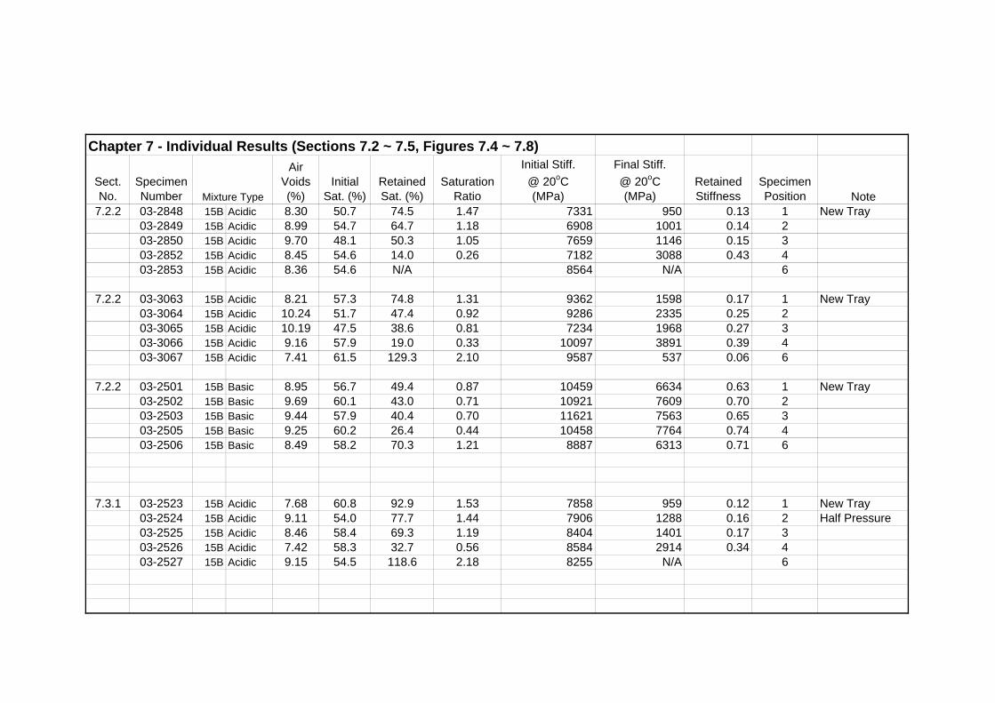
Chapter 7 - Individual Results (Sections 7.2 ~ 7.5, Figures 7.4 ~ 7.8)

Sect.No.

SpecimenNumber

Air Voids(%)

InitialSat. (%)

RetainedSat. (%)

Saturation Ratio

Initial Stiff.@ 20oC(MPa)

Final Stiff.@ 20oC(MPa)

RetainedStiffness

SpecimenPosition Note

7.2.2 03-2848 15B Acidic 8.30 50.7 74.5 1.47 7331 950 0.13 1 New Tray03-2849 15B Acidic 8.99 54.7 64.7 1.18 6908 1001 0.14 203-2850 15B Acidic 9.70 48.1 50.3 1.05 7659 1146 0.15 303-2852 15B Acidic 8.45 54.6 14.0 0.26 7182 3088 0.43 403-2853 15B Acidic 8.36 54.6 N/A 8564 N/A 6

7.2.2 03-3063 15B Acidic 8.21 57.3 74.8 1.31 9362 1598 0.17 1 New Tray03-3064 15B Acidic 10.24 51.7 47.4 0.92 9286 2335 0.25 203-3065 15B Acidic 10.19 47.5 38.6 0.81 7234 1968 0.27 303-3066 15B Acidic 9.16 57.9 19.0 0.33 10097 3891 0.39 403-3067 15B Acidic 7.41 61.5 129.3 2.10 9587 537 0.06 6

7.2.2 03-2501 15B Basic 8.95 56.7 49.4 0.87 10459 6634 0.63 1 New Tray03-2502 15B Basic 9.69 60.1 43.0 0.71 10921 7609 0.70 203-2503 15B Basic 9.44 57.9 40.4 0.70 11621 7563 0.65 303-2505 15B Basic 9.25 60.2 26.4 0.44 10458 7764 0.74 403-2506 15B Basic 8.49 58.2 70.3 1.21 8887 6313 0.71 6

7.3.1 03-2523 15B Acidic 7.68 60.8 92.9 1.53 7858 959 0.12 1 New Tray03-2524 15B Acidic 9.11 54.0 77.7 1.44 7906 1288 0.16 2 Half Pressure03-2525 15B Acidic 8.46 58.4 69.3 1.19 8404 1401 0.17 303-2526 15B Acidic 7.42 58.3 32.7 0.56 8584 2914 0.34 403-2527 15B Acidic 9.15 54.5 118.6 2.18 8255 N/A 6

Mixture Type

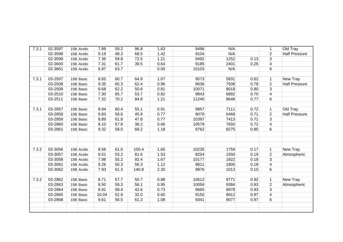
7.3.1 02-3597 15B Acidic 7.89 59.2 96.8 1.63 9496 N/A 1 Old Tray02-3598 15B Acidic 9.19 48.3 68.5 1.42 9104 N/A 2 Half Pressure02-3599 15B Acidic 7.36 59.8 72.5 1.21 9492 1252 0.13 302-3600 15B Acidic 7.31 61.7 39.5 0.64 9185 2401 0.26 402-3601 15B Acidic 6.97 63.7 0.00 10103 N/A 6

7.3.1 03-2507 15B Basic 8.65 60.7 64.9 1.07 9573 5931 0.62 1 New Tray03-2508 15B Basic 9.35 65.3 62.4 0.96 9636 7508 0.78 2 Half Pressure03-2509 15B Basic 9.68 62.2 50.6 0.81 10071 8018 0.80 303-2510 15B Basic 7.30 65.7 53.7 0.82 9843 6892 0.70 403-2511 15B Basic 7.32 70.2 84.8 1.21 11240 8648 0.77 6

7.3.1 03-2857 15B Basic 8.94 60.4 55.1 0.91 9857 7111 0.72 1 Old Tray03-2858 15B Basic 9.83 59.6 45.9 0.77 9079 6468 0.71 2 Half Pressure03-2859 15B Basic 8.89 61.8 47.8 0.77 10397 7413 0.71 303-2860 15B Basic 8.10 57.8 38.2 0.66 10579 7650 0.72 403-2861 15B Basic 9.32 58.0 68.2 1.18 9762 8275 0.85 6

7.3.2 03-3056 15B Acidic 8.56 61.0 100.4 1.65 10235 1759 0.17 1 New Tray03-3057 15B Acidic 9.51 53.2 81.6 1.53 8254 1550 0.19 2 Atmospheric03-3058 15B Acidic 7.98 55.2 92.4 1.67 10177 1822 0.18 303-3061 15B Acidic 9.26 50.3 56.3 1.12 9811 1800 0.18 403-3062 15B Acidic 7.93 61.3 140.8 2.30 9876 1013 0.10 6

7.3.2 03-2862 15B Basic 8.71 57.7 50.7 0.88 10612 9771 0.92 1 New Tray03-2863 15B Basic 8.50 59.3 56.1 0.95 10059 9384 0.93 2 Atmospheric03-2864 15B Basic 8.91 58.4 42.6 0.73 9665 8978 0.93 303-2865 15B Basic 10.04 52.9 32.0 0.60 9150 8912 0.97 403-2868 15B Basic 9.61 56.5 61.3 1.08 9341 9077 0.97 6

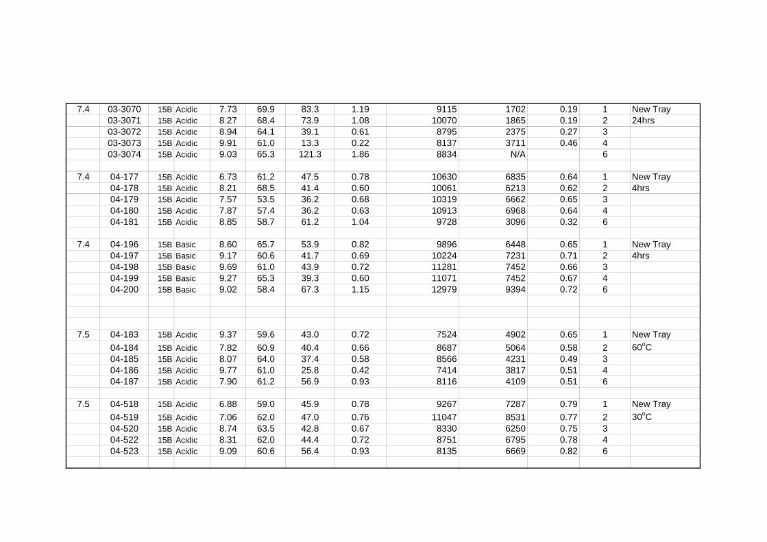
7.4 03-3070 15B Acidic 7.73 69.9 83.3 1.19 9115 1702 0.19 1 New Tray03-3071 15B Acidic 8.27 68.4 73.9 1.08 10070 1865 0.19 2 24hrs03-3072 15B Acidic 8.94 64.1 39.1 0.61 8795 2375 0.27 303-3073 15B Acidic 9.91 61.0 13.3 0.22 8137 3711 0.46 403-3074 15B Acidic 9.03 65.3 121.3 1.86 8834 N/A 6

7.4 04-177 15B Acidic 6.73 61.2 47.5 0.78 10630 6835 0.64 1 New Tray04-178 15B Acidic 8.21 68.5 41.4 0.60 10061 6213 0.62 2 4hrs04-179 15B Acidic 7.57 53.5 36.2 0.68 10319 6662 0.65 304-180 15B Acidic 7.87 57.4 36.2 0.63 10913 6968 0.64 404-181 15B Acidic 8.85 58.7 61.2 1.04 9728 3096 0.32 6

7.4 04-196 15B Basic 8.60 65.7 53.9 0.82 9896 6448 0.65 1 New Tray04-197 15B Basic 9.17 60.6 41.7 0.69 10224 7231 0.71 2 4hrs04-198 15B Basic 9.69 61.0 43.9 0.72 11281 7452 0.66 304-199 15B Basic 9.27 65.3 39.3 0.60 11071 7452 0.67 404-200 15B Basic 9.02 58.4 67.3 1.15 12979 9394 0.72 6

7.5 04-183 15B Acidic 9.37 59.6 43.0 0.72 7524 4902 0.65 1 New Tray04-184 15B Acidic 7.82 60.9 40.4 0.66 8687 5064 0.58 2 60oC04-185 15B Acidic 8.07 64.0 37.4 0.58 8566 4231 0.49 304-186 15B Acidic 9.77 61.0 25.8 0.42 7414 3817 0.51 404-187 15B Acidic 7.90 61.2 56.9 0.93 8116 4109 0.51 6

7.5 04-518 15B Acidic 6.88 59.0 45.9 0.78 9267 7287 0.79 1 New Tray04-519 15B Acidic 7.06 62.0 47.0 0.76 11047 8531 0.77 2 30oC04-520 15B Acidic 8.74 63.5 42.8 0.67 8330 6250 0.75 304-522 15B Acidic 8.31 62.0 44.4 0.72 8751 6795 0.78 404-523 15B Acidic 9.09 60.6 56.4 0.93 8135 6669 0.82 6

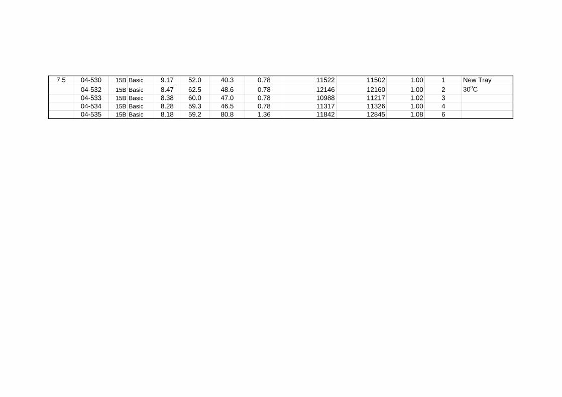
7.5 04-530 15B Basic 9.17 52.0 40.3 0.78 11522 11502 1.00 1 New Tray04-532 15B Basic 8.47 62.5 48.6 0.78 12146 12160 1.00 2 30oC04-533 15B Basic 8.38 60.0 47.0 0.78 10988 11217 1.02 304-534 15B Basic 8.28 59.3 46.5 0.78 11317 11326 1.00 404-535 15B Basic 8.18 59.2 80.8 1.36 11842 12845 1.08 6

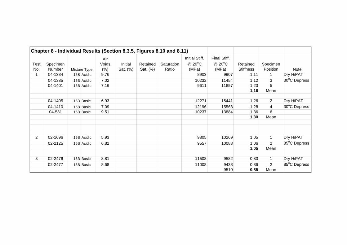
Chapter 8 - Individual Results (Section 8.3.5, Figures 8.10 and 8.11)

TestNo.

SpecimenNumber

AirVoids(%)

InitialSat. (%)

RetainedSat. (%)

Saturation Ratio

Initial Stiff.@ 20oC(MPa)

Final Stiff.@ 20oC(MPa)

RetainedStiffness

SpecimenPosition Note

1 04-1384 15B Acidic 9.76 8903 9907 1.11 1 Dry HiPAT04-1385 15B Acidic 7.02 10232 11454 1.12 3 30oC Depress04-1401 15B Acidic 7.16 9611 11857 1.23 5

1.16 Mean

04-1405 15B Basic 6.93 12271 15441 1.26 2 Dry HiPAT04-1410 15B Basic 7.09 12196 15563 1.28 4 30oC Depress04-531 15B Basic 9.51 10237 13884 1.36 6

1.30 Mean

2 02-1696 15B Acidic 5.93 9805 10269 1.05 1 Dry HiPAT02-2125 15B Acidic 6.82 9557 10083 1.06 2 85oC Depress

1.05 Mean

3 02-2476 15B Basic 8.81 11508 9582 0.83 1 Dry HiPAT02-2477 15B Basic 8.68 11008 9438 0.86 2 85oC Depress

9510 0.85 Mean

Mixture Type

F.12

NG953 (08/04) Method for the Assessment of Durability of Compacted Asphalt Mixtures using the Saturation Ageing Tensile Stiffness (SATS) Test 1 The test method is intended to simulate the combined effect of ageing and

moisture on asphalt pavement materials in service. It is suitable for coated macadam

base and binder course mixtures with a nominal (water accessible) air void content

of 8% and a nominal binder content of 4%. The test may not be suitable for mixtures

of high binder content or manufactured with binders of penetration greater than 50.

2 Clause 953 incorporates by dated or undated reference, provisions from other

publications. These normative references are cited at the appropriate places in the

text, and the publications are listed in Appendix F. For dated references, subsequent

amendments to or revisions of any of these publications apply to this Clause only

when incorporated in it by amendment or revision. For undated references the latest

edition of the publication referred to applies (including amendments).

3 Recent evidence from an early demonstration trial of High Modulus Base (HMB)

materials in the UK showed an unexpected drop in material stiffness modulus (up to

60%) only a few years after construction. Other investigations into HMB materials

that have been used for in-service pavements generally showed better performance,

although some also displayed unexpected decreases in the stiffness modulus of the

HMB material. It is thought that the sensitivity of the material to ageing and

moisture is of key importance in helping to explain this behaviour. The main

purpose of the SATS test is to reproduce in the laboratory the decrease in stiffness

modulus that had been measured from the HMB trial site, so that unsuitable

aggregate/binder combinations are screened out at mixture design stage.

4 With reference to sub-Clause 953.4 (ii), 100 mm wide ‘Foil-faced self-adhesive

tape’ supplied by IDENT, has been found to be suitable. The tape can be obtained

from WR Thermal Contracts, 1 Ludlam Avenue, Giltbrook, Nottingham, NG16 2UL

(Tel: 07775 646 526).

F.13

5 With reference to sub-Clause 953.5 (v), a 100 mm diameter, 5 mm thick rigid

porous disc for use with a standard soils triaxial cell as described in Clause 3.2 (g) of

BS 1377: Part 8: 1990, has been found to be suitable.

6 The form and dimensions of the pressure vessel and specimen tray shown in

Figures 9/9 and 9/10 have been found to yield repeatable results in the SATS test

when used with two different aggregate types. Other forms of pressure vessel and

specimen tray may also be suitable, but have not been specifically investigated.

However, early work carried out in a standard binder pressure ageing vessel to

AASHTO PP1 yielded similar results to those generated using the apparatus

described in Clause 953.

7 The standard SATS test involves specimens cored from a slab manufactured

using a laboratory roller compactor. Specimens for test may also be cored from an

in-service pavement in accordance with BS 598-100, but research data on the

performance of such specimens in the SATS test is not currently available.

8 The measurement of density on sealed specimens is considered essential for

material with an air void content of 8%. Wax is not suitable as a sealing material

since it is practically impossible to remove from specimens that will be subjected to

subsequent mechanical testing. The self-adhesive aluminium foil described in sub-

Clause NG 953.4 above has been successfully used in a number of laboratories in the

UK for over 10 years, and is easy to remove. For laboratory prepared specimens

with a rough surface texture, the foil may cause observation of texture voids as

internal specimen voids, which may cause an under-estimation of the specimen

density and an over-estimation of the air voids level of the specimen. However, the

risk of this is considered to be relatively small in the SATS test specimens, which are

normally cored from a laboratory manufactured slab and then trimmed (sawn) to the

specified thickness.

9 The test temperature of 85°C and test duration of 65 hours are the same as those

adopted for the High Pressure Ageing Test (HiPAT) developed for BBA/HAPAS

(British Board of Agrément/Highway Authorities Product Approval Scheme)

Specialist Group (SG) 4 for Modified Binders. The reduced temperature compared

F.14

with the standard conditions described in AASHTO PP1 was used to reduce the

difference between test temperature and service temperature, with the extended time

incorporated in compensation.

10 With reference to sub-Clause 953.16, the additional cooling period is applied to

reduce the pressure related damage during the depressurising process. Normally the

target temperature (30oC) can be achieved within 24 hours. It should be noted that

the pressure needs to be carefully maintained during this cooling process, as the

reducing temperature will reduce the vessel pressure accordingly. This can be

achieved by carefully setup the pressure input controlling valve to just below the

target pressure (2.1 MPa), thus any gradual lose of pressure will be automatically

compensated by the gradual input of the pressure from the compressed air cylinder.

11 It was found during the development of the HiPAT that it was necessary to

reduce pressure slowly, to avoid excessive foaming of binder due to release of

dissolved air. A similar slow release of pressure is recommended at the end of the

SATS conditioning procedure, to reduce damage to the specimens as a result of

sudden changes of pressure. The influence of the method of pressure release in the

test is the subject of ongoing research.

12 With reference to sub-Clause 953.18, 3 minutes has been found to be a practical

time period to complete the surface drying and weighing of all five specimens after

removal from the pressure vessel. Any reduction in this time period (below

3 minutes) should help to improve the precision of the test.

13 Figure NG 9/1 shows a suitable format for the graphical representation of the

stiffness ratio versus saturation value plot. The data shown in the figure are

examples only. Acceptable values for stiffness ratio at a given saturation after

conditioning, for a mixture to be considered not susceptible to the combined effect of

ageing and moisture in service, are the subject of ongoing research.

14 The precision for the SATS test method has not been established.

F.15

Figure NG 9/1: (08/04) Graphical Representation of Typical Stiffness/Saturation Data

0.0

0.2

0.4

0.6

0.8

1.0

1.2

0 20 40 60 80 100 120

Saturation after Conditioning(%)

Stiff

ness

Rat

io

Immersed Specimen (5th Position, Bottom)

4th Position

1st Position (Top)

3rd Position

2nd Position

F.1

953 (08/04) Method for the Assessment of Durability of Compacted Asphalt Mixtures using the Saturation Ageing Tensile Stiffness (SATS) Test

Scope

1 This Clause specifies a test method to assess the sensitivity of asphalt pavement

materials to a combined ageing/moisture sensitivity procedure, by measuring

stiffness before and after the test. The test is known as the Saturation Ageing Tensile

Stiffness (SATS) test.

Terms and Definitions

2 For the purposes of this Clause the terms and definitions given in BS 6100 shall

apply, together with the following.

(i) Maximum Density

Mass per unit volume, without air voids, of a bituminous mixture at known

test temperature.

(ii) Dry Bulk Density

Mass per unit volume, including the air voids, of a specimen at known test

temperature.

(iii) Saturation Before Conditioning

The saturation of the mixture, determined as the calculated percentage of air

voids filled with water after partial vacuum saturation, prior to conditioning

as described in this Clause.

(iv) Unconditioned Stiffness

The stiffness modulus of the mixture as determined in accordance with BS

DD 213:1993, prior to conditioning as described in this Clause.

F.2

(v) Conditioned Stiffness

The stiffness modulus of the mixture as determined in accordance with BS

DD 213:1993, after conditioning as described in this Clause.

(vi) Stiffness Ratio

The ratio of the conditioned stiffness to the unconditioned stiffness

(vii) Saturation After Conditioning

The saturation of the mixture, determined as the calculated percentage of air

voids filled with water after conditioning as described in this Clause.

Principle of Test

3 Nominally identical test specimens shall be subjected to moisture saturation by

using a vacuum system. They shall then be transferred into a pressurised vessel

partially filled with water, where they shall be subjected to a conditioning procedure

at 85°C temperature and 2.1 MPa pressure for 65 hours. The stiffness ratio of

individual specimens shall be plotted against their percentage saturation after

conditioning to determine the sensitivity of the material to ageing and moisture. The

whole process is referred to as the Saturation Ageing Tensile Stiffness (SATS) test.

Materials

4 The following materials shall be used:

(i) Distilled water, freshly de-aired and cooled.

(ii) Self-adhesive aluminium foil: Capable of adhering to and covering the

specimen with an impervious coating.

(iii) Absorbent paper towelling.

F.3

Test Apparatus

5 The following test apparatus shall be used:

(i) Vacuum desiccator and vacuum pump, including manometer or calibrated

vacuum gauge as described in BS EN 12697-5.

(ii) Balance with sufficient capacity and accurate to 1.0 g.

(iii) Pressure Vessel having the form and dimensions specified in Figure 9/9,

similar to that described in AASHTO PP1, and of sufficient capacity to

accommodate 5 test specimens, of dimensions as described in sub-Clause 6

of this Clause, for a full test.

(iv) Test equipment capable of performing the Indirect Tensile Stiffness

Modulus (ITSM) test on compacted bituminous mixture specimens in

accordance with BS DD 213.

(v) Specimen tray, having the form and dimensions specified in Figure 9/10, to

accommodate five test specimens for a full test. The tray shall sit in the

pressure vessel on top of a porous disc as shown in Figure 9/11.

Sample Preparation

6 Test specimens shall be cores of 100 + 0, -5 mm diameter and 60 ± 5 mm

thickness. Specimens shall be cored from a slab manufactured using a laboratory

roller compactor in accordance with prEN12697-33. Five nominally identical

specimens are required for the full test.

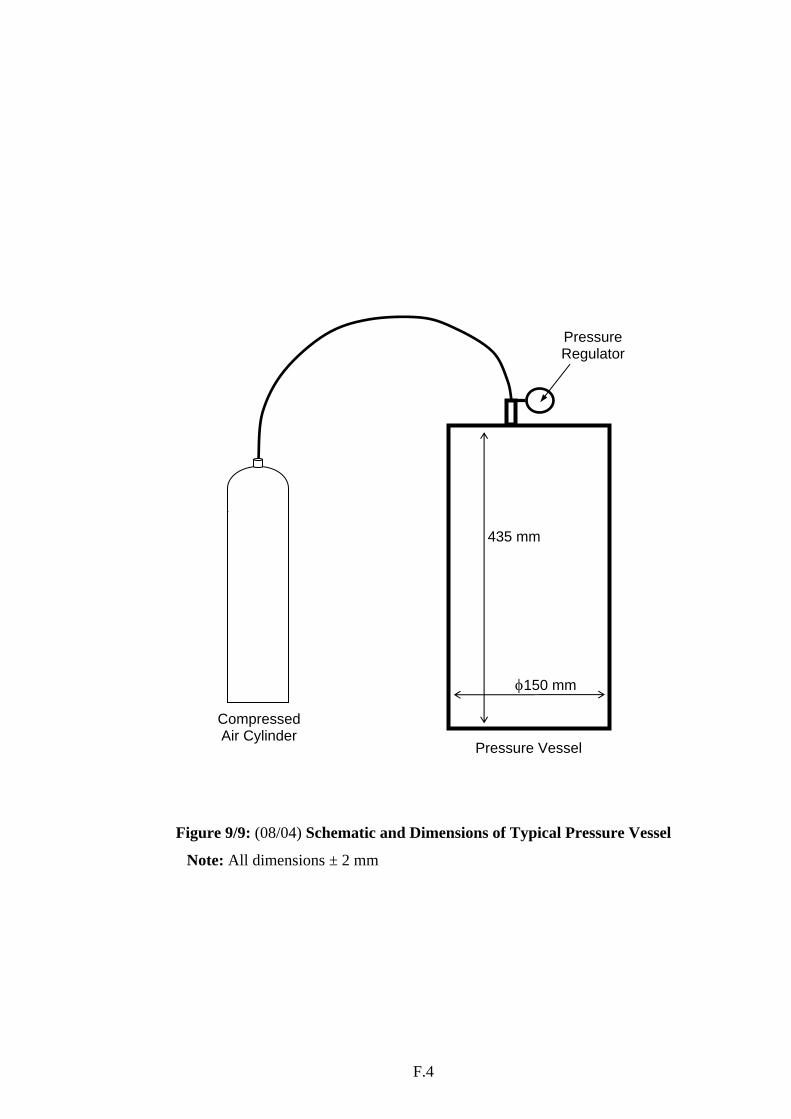
F.4

Figure 9/9: (08/04) Schematic and Dimensions of Typical Pressure Vessel

Note: All dimensions ± 2 mm

Pressure Vessel

φ150 mm

435 mm

Pressure Regulator

Compressed Air Cylinder

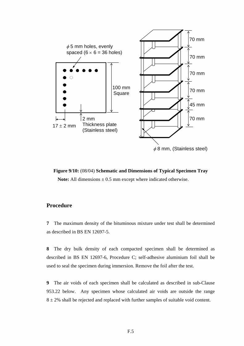
F.5

Figure 9/10: (08/04) Schematic and Dimensions of Typical Specimen Tray

Note: All dimensions ± 0.5 mm except where indicated otherwise.

Procedure

7 The maximum density of the bituminous mixture under test shall be determined

as described in BS EN 12697-5.

8 The dry bulk density of each compacted specimen shall be determined as

described in BS EN 12697-6, Procedure C; self-adhesive aluminium foil shall be

used to seal the specimen during immersion. Remove the foil after the test.

9 The air voids of each specimen shall be calculated as described in sub-Clause

953.22 below. Any specimen whose calculated air voids are outside the range

8 ± 2% shall be rejected and replaced with further samples of suitable void content.

45 mm

70 mm

70 mm

70 mm

70 mm

70 mm

φ 8 mm, (Stainless steel)

φ 5 mm holes, evenly spaced (6 × 6 = 36 holes)

100 mm Square

2 mm Thickness plate (Stainless steel)

17 ± 2 mm

F.6

10 The unconditioned (initial) stiffness modulus shall be determined at 20 ± 0.5°C

in the NAT. Designate this as ITSMU.

11 Determine the dry mass of each specimen using the balance and designate this as

Md.

12 The specimens shall be partially saturated by placing them in the vacuum

desiccator, covering them with distilled water at 20 ± 1°C, sealing the apparatus, and

applying a partial vacuum pressure of 68 ± 3 kPa for 30 minutes.

13 Remove each specimen from the vacuum desiccator, remove any water on its

surface using the absorbent paper towelling and determine its wet mass. Designate

this as Mw. The percent saturation (S) shall be determined as described in sub-

Clause 953.23 below. Any specimens whose calculated saturation is ≥ 80% shall be

rejected.

14 Partly fill the pressure vessel with water. The water level shall be between the

4th and 5th specimen after loading the samples, as shown in Figure 9/11. Freshly

distilled water only shall be used (do not re-use). The vessel and water shall be

controlled to the target temperature for at least 2 hours before the conditioning

procedure commences.

15 The specimens shall be placed into the vessel, using the specimen tray, the cover

closed and the pressure gradually increased from atmospheric pressure to 2.1 MPa

over a period of 20 minutes. The conditioning procedure shall then be performed, as

described in AASHTO PP1, at 2.1 ± 0.1 MPa pressure and the target temperature of

85 ± 1°C for 65 ± 1h.

16 After the test period of 65 hrs has elapsed, adjust the target temperature to 30oC.

Leave the vessel for the natural cooling for another 24 hrs (Do not release the

pressure yet).

F.7

17 When the pressure vessel display temperature has reduced to 30°C (after the

additional 24 hrs cooling period), the pressure slowly released from the vessel. The

pressure release mechanism shall be adjusted so that the pressure returns to

atmospheric pressure over a period of 20 to 30 minutes (linear reduction). The cover

shall be opened and all the specimens extracted, on the tray, from the vessel.

18 Each specimen shall be surface dried using the absorbent paper towelling, and its

wet mass measured within 3 minutes of removing the specimens from the pressure

vessel. Designate this mass as Mw2. The saturation after the conditioning procedure

(Sa) shall be calculated as described in sub-Clause 953.24 below.

19 The specimens shall be observed for any visual cracks and unusual appearance

(i.e. colour of binder or aggregates). Record any comments as appropriate.

20 The specimens shall be placed into the NAT or other suitable temperature

controlled conditioning environment at 20 ± 0.5°C in preparation for ITSM testing,

as described in BS DD 213.

21 The stiffness modulus shall be determined as described in BS DD 213 within

8 hrs after releasing the pressure from the vessel. Designate this as ITSMC.

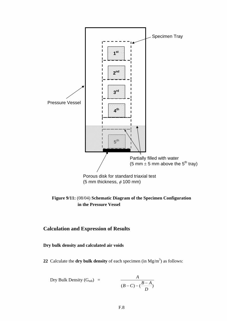
F.8

Figure 9/11: (08/04) Schematic Diagram of the Specimen Configuration in the Pressure Vessel

Calculation and Expression of Results

Dry bulk density and calculated air voids

22 Calculate the dry bulk density of each specimen (in Mg/m3) as follows:

Dry Bulk Density (Gmb) = )()(

DABCB

A−

−−

1st

2nd

3rd

4th

5th

Specimen Tray

Partially filled with water (5 mm ± 5 mm above the 5th tray)

Pressure Vessel

Porous disk for standard triaxial test (5 mm thickness, φ 100 mm)

F.9

where: A = the mass of the dry specimen in air (in g) B = the mass of the coated specimen in air (in g) C = the mass of the coated specimen in water (in g) D = the density* of the self-adhesive aluminium foil in Mg/m³

* The material described in sub-Clause 953.4 (ii) has been found to have a typical

density of 1.650Mg/m³

The specimen dry bulk density shall be expressed to the nearest 0.001Mg/m³

The air voids of each specimen (in %) shall be calculated as follows:

Air Voids = 100×−mm

mbmm

GGG

where:

Gmm is the maximum density determined in accordance with BS EN 12697-5 Gmb is the dry bulk density determined in accordance with BS EN 12697-6,

Procedure C.

The calculated air voids shall be expressed to the nearest 0.1%.

Saturation before conditioning

23 Calculate the saturation before conditioning as follows:

100×−

−=

mm

d

mb

d

dw

GM

GM

MMS

where: S = percent saturation before conditioning Md = mass of dry specimen, g

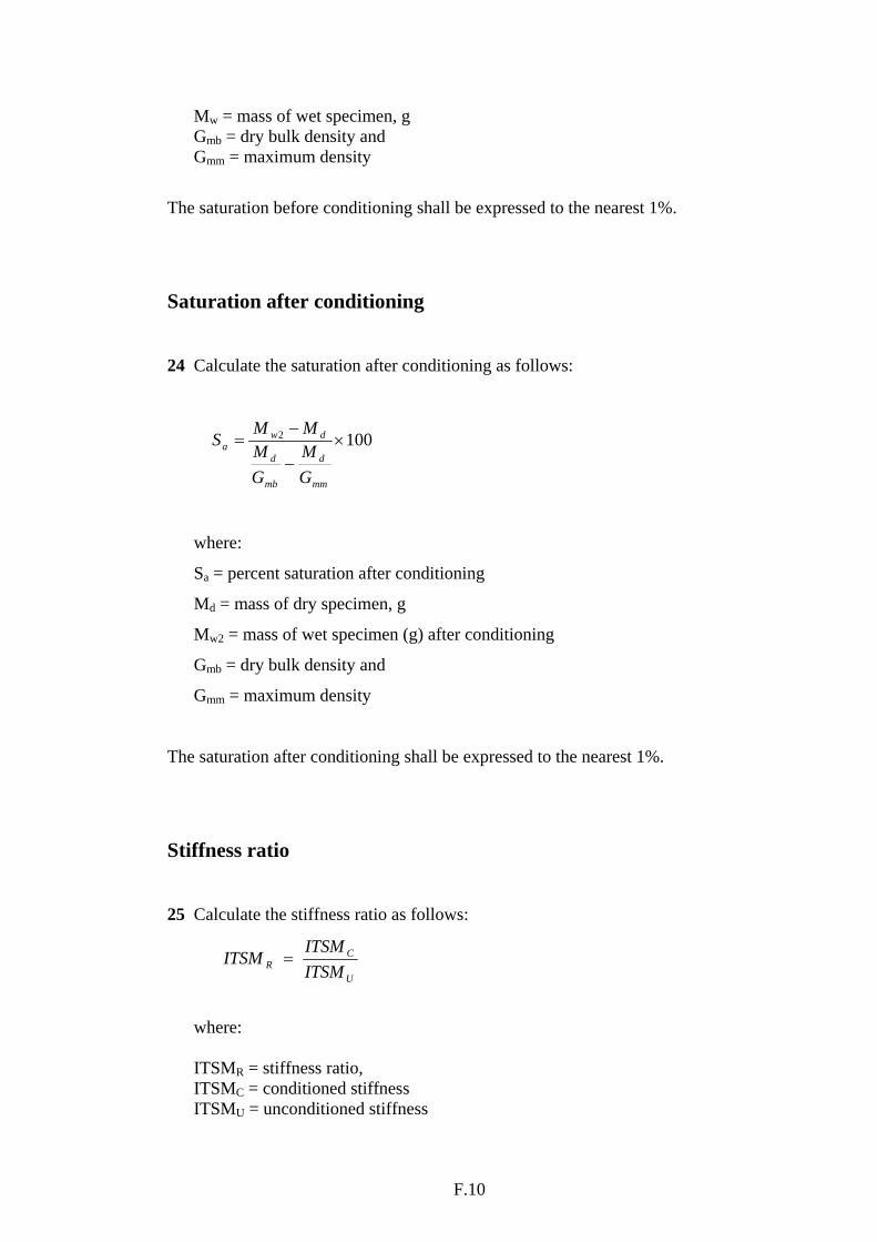
F.10

Mw = mass of wet specimen, g Gmb = dry bulk density and Gmm = maximum density

The saturation before conditioning shall be expressed to the nearest 1%.

Saturation after conditioning

24 Calculate the saturation after conditioning as follows:

1002 ×−

−=

mm

d

mb

d

dwa

GM

GM

MMS

where:

Sa = percent saturation after conditioning

Md = mass of dry specimen, g

Mw2 = mass of wet specimen (g) after conditioning

Gmb = dry bulk density and

Gmm = maximum density

The saturation after conditioning shall be expressed to the nearest 1%.

Stiffness ratio

25 Calculate the stiffness ratio as follows:

U

CR ITSM

ITSMITSM =

where: ITSMR = stiffness ratio, ITSMC = conditioned stiffness ITSMU = unconditioned stiffness

F.11

The stiffness ratio shall be expressed to the nearest 0.01.

Test Report

26 The test report shall contain not less than the following information:

a) A reference to this test method and test conditions.

b) Maximum density of the mixture tested, to the nearest 0.001 Mg/m³.

c) For each specimen tested, report:

- Dry bulk density (Gmb), to the nearest 0.001 Mg/m³.

- Percent air voids (Vv), to the nearest 0.1%.

- Percent saturation (S) before conditioning, to the nearest 1%.

- Percent saturation after conditioning, (Sa), to the nearest 1%.

- Unconditioned stiffness (ITSMU) before conditioning, to the nearest 100 MPa.

- Conditioned stiffness (ITSMC) after conditioning, to the nearest 100 MPa.

- Stiffness ratio (ITSMR), to the nearest 0.01.

- Any cracks or unusual appearance.

d) For the mixture tested, the stiffness ratio of the individual specimens tested

shall be plotted against the corresponding saturation value after

conditioning. The graph shall have linear axes for stiffness ratio (y axis)

and saturation after conditioning (x axis). The scales of the graph shall

cover a range of stiffness ratio of at least 0 - 1.0 and of saturation after

conditioning of 0 - 100%.

27 The test report and graph, uniquely identified, shall be provided to the

Overseeing Organisation with the Contractor’s Proposal.