Chirality Transfer from Chiral Solutes and

Surfaces to Achiral Solvents: Insights from

Molecular Dynamics Studies

by

Shihao Wang

A thesis submitted to the Department of Chemistry

in conformity with the requirements for

the degree of Doctor of Philosophy

Queen’s University

Kingston, Ontario, Canada

(September, 2009)

Copyright © Shihao Wang, 2009

ii

Abstract

Chirality can be induced in achiral solvent molecules located near a chiral

molecule or surface, but there have been very few systematic studies in this field either

experimentally or theoretically. The focus of this thesis is to study the chirality transfer

from chiral molecules to achiral solvents.

To capture the chirality transfer in solvent molecules, a solvent model that is

sensitive to the changes in the environment is needed. We developed new polarizable

and flexible models based on an extensive series of ab initio calculations and molecular

dynamics simulations. The models include electric field dependence in both the atomic

charges and the intramolecular degrees of freedom. Modified equations of motion are

required and we have implemented a multiple time step algorithm to solve these

equations. Our methodology is general and has been applied to ethanol as a test. For

other solvents in our simulations, such as 2-propanol, limited models are used.

The chirality transfer from chiral solutes to achiral solvents and its dependence on

the solute and solvent characteristics are then explored using the new polarizable models

in molecular dynamics simulations. The chirality induced in the solvent is assessed based

on a series of related chirality indexes originally proposed by Osipov[Osipov et al., Mol.

Phys.84, 1193(1995)]. Two solvents are considered: Ethanol and benzyl alcohol. The

solvation of three chiral solutes is examined: Styrene oxide, acenaphthenol, and n-(1-(4-

bromophenyl)ethyl)pivalamide (PAMD). All three solutes have the possibility of

hydrogen-bonding with the solvent, the last two may also form π-π interactions, and the

last has multiple hydrogen bonding sites.

iii

The chirality transfer from chiral surfaces to achiral solvents is also explored.

Emphasis is placed on the extent of this chirality transfer and its dependence on the

surface and solvent characteristics is explored. Three surfaces employed in chiral

chromatography are examined: The Whelk-O1 interface; a phenylglycine-derived chiral

stationary phase (CSP); and a leucine-derived CSP. The solvents consist of ethanol, a

binary n-hexane/ethanol solvent, 2-propanol, and a binary n-hexane/2-propanol solvent.

Molecular dynamics simulations of the solvated chiral interfaces form the basis of the

analysis and position dependent chirality indexes are analyzed in detail.

iv

Acknowledgements

First, I would like to thank my supervisor, Dr. Natalie Cann, for providing me

with excellent advice throughout my graduate work. Without her help, this thesis and the

work within would never have been completed. I would also like to thank Dr. Gang Wu,

and Dr. Derek Pratt, for their guidance at my supervisory committee meetings. Many

thanks to all members of the Cann group: Dr. Sorin Nita, Dr. Chunfeng Zhao, Rodica

Pecheanu, and Mohammad Ashtari, for providing a great working environment.

I would like to thank all my friends for the support and encouragement I received

outside of Chernoff Hall. I am also grateful to my parents, who have always been there

when I needed them. A special thanks to my fiancée, Fang Gao, for her love, support and

understanding.

The last but not the least, financial support from NSERC, Queen’s University, and

HPCVL scholarships, and computing facilities on SHARCNET, WESTGRID and

HPCVL are gratefully acknowledged.

v

Statement of Originality

I hereby certify that all of the work described within this thesis is the original work of the

author under the supervision of Professor Natalie Cann. Any published (or unpublished)

ideas and/or techniques from the work of others are fully acknowledged in accordance

with the standard referencing practices.

Shihao Wang

September, 2009

vi

Table of Contents

 Abstract .............................................................................................................................. ii

Acknowledgements .......................................................................................................... iv

Statement of Originality ................................................................................................... v

Table of Contents ............................................................................................................. vi

List of Tables .................................................................................................................... xi

List of Figures .................................................................................................................. xii

List of Abbreviations ...................................................................................................... xv

Chapter 1 Introduction................................................................................................... 1

1.1 Introduction to chirality ............................................................................................ 1

1.2 Studies on chirality transfer ...................................................................................... 3

1.3 Polarizable models .................................................................................................... 7

1.4 Measuring chirality ................................................................................................. 11

1.5 Thesis organization ................................................................................................. 15

Chapter 2 Theoretical Methods and Models .............................................................. 16

2.1 Molecular dynamics simulations ............................................................................ 16

2.1.1 Potentials ......................................................................................................... 17

2.1.2 Periodic Boundary Conditions ........................................................................ 23

vii

2.1.3 Ewald summation............................................................................................ 25

2.2 Polarizable Models.................................................................................................. 29

2.2.1 Fluctuating Charge Model ............................................................................... 29

2.2.2 Fluctuating Charge and INTRAmolecular potential model ............................. 32

2.3 Equations of motion ................................................................................................ 37

2.3.1 Verlet Algorithms ............................................................................................ 37

2.3.2 Nosé-Hoover Thermostat ................................................................................. 39

2.4 Reversible Multiple Time Step MD ........................................................................ 42

2.5 Quantum Mechanics Methods ................................................................................ 48

2.5.1 Ab initio calculations........................................................................................ 48

2.5.2 Density function theory .................................................................................... 49

2.5.3 Basis sets .......................................................................................................... 51

2.5.4 Atomic charges ................................................................................................ 53

2.5.5 Conformational Minimization ......................................................................... 54

2.6 Chirality indexes ..................................................................................................... 55

2.7 Surface representations ........................................................................................... 58

2.8 Practical considerations .......................................................................................... 62

Chapter 3 Development of a polarizable and flexible model .................................... 64

3.1 Introduction ............................................................................................................. 64

3.2. Methods.................................................................................................................. 67

viii

3.2.1 Assessment of typical electric fields in bulk ethanol ....................................... 69

3.2.2 Ab initio calculations for molecular response ................................................. 70

3.2.3 Fluctuating Charge Model ............................................................................... 74

3.2.4 Lennard-Jones potentials ................................................................................ 77

3.2.5 Intramolecular potentials ................................................................................. 77

3.2.6 Simulation details ............................................................................................. 86

3.3. Results and discussion ........................................................................................... 93

3.3.1 Bulk ethanol ..................................................................................................... 93

3.3.2 Hydrogen bonding ......................................................................................... 100

3.4. Conclusions .......................................................................................................... 102

Chapter 4 Chirality transfer: The impact of a chiral solute on an achiral solvent

......................................................................................................................................... 105

4.1. Introduction .......................................................................................................... 105

4.2. Methods................................................................................................................ 108

4.2.1 Solvent and solute models ............................................................................. 108

4.2.2 The assessment of chirality ............................................................................ 113

4.2.3. Simulation details ......................................................................................... 118

4.2.4 Convergence of the chirality transfer ............................................................. 120

4.3. Results and discussion ........................................................................................ 125

4.3.1 Analyte solvation ........................................................................................... 125

ix

4.3.2 The solvent representation: Is polarizability important? .............................. 129

4.3.3 Chirality transfer and conformational averaging. .......................................... 132

4.3.4 Contact points and chirality transfer. ............................................................. 138

4.4. Conclusions ......................................................................................................... 144

Chapter 5 Chirality transfer from chiral surfaces to nearby solvents ................... 146

5.1. Introduction .......................................................................................................... 146

5.2. Methods................................................................................................................ 149

5.2.1 Surface representations .................................................................................. 149

5.2.2 Models............................................................................................................ 149

5.2.3 Chirality indexes ............................................................................................ 151

5.2.4 Simulation details ........................................................................................... 155

5.3. Results and discussion ......................................................................................... 157

5.3.1 Solvation of Chiral Stationary Phases ............................................................ 158

5.3.2 Chirality transfer at interfaces ........................................................................ 165

5.3.3 Comparisons between selectors: Conformational chirality .......................... 168

5.3.4 Comparisons between selectors: Solvent polarization .................................. 175

5.3.5 Comparison of different solvents ................................................................... 179

5.4. Conclusions .......................................................................................................... 182

Chapter 6 Conclusions ................................................................................................ 184

Bibliography .................................................................................................................. 189

x

APPENDIX A Evaluation of charge fluctuation parameters 0~iχ and iζ . ........ 200

APPENDIX B Evaluation of forces ........................................................................... 205

APPENDIX C Details of the potentials for 2-propanol ........................................... 212

xi

List of Tables Table 3.1. Average error in the dipole moment, relative to MP2/aug-cc-pVTZ reference calculations (see Eq. [3.2]), for ethanol in 16 electric fields. . ......................................... 73 

Table 3.2. Charge fluctuation parameters (see Eq. [2.25]) and Lennard-Jones parameters for the polarizable, flexible fCINTRA ethanol model. ..................................................... 75 

Table 3.3. The zero-field bond stretching constants and the field dependence of the equilibrium bond lengths (see Eq. [2.31]) extracted from B3LYP/6-311++G(d,p) calculations of ethanol. ..................................................................................................... 79 

Table 3.4. The zero-field angle bending force constant and the field dependence of the equilibrium bond angles (see Eq. [2.32]) extracted from B3LYP/6-311++G(d,p) calculations of ethanol. ..................................................................................................... 82 

Table 3.5. Field dependence of the torsional coefficients for rotation about the C(3)-O(2) bond in ethanol (see Eq. [2.33]). ....................................................................................... 84 

Table 3.6. Properties of bulk ethanol as predicted from the polarizable, flexible fCINTRA model are compared with experiment. ............................................................. 95 

Table 3.7. Hydrogen bond statistics evaluated from snapshots of the simulation cell.. 101 

Table 4.1. Intramolecular potential parameters for benzyl alcohol.. ............................. 110 

Table 4.2. Charge fluctuation parameters (see Eq. [2.26]) and zero-field charges for benzyl alcohol. ................................................................................................................ 112 

Table 4.3. An analysis of solvent hydrogen-bonding and the average chirality of the solutes. ............................................................................................................................ 128 

Table 4.4. Average excess chirality for solvent around chiral solute. .......................... 136 

Table 4.5. Average excess chirality for solvent hydrogen bonded to the chiral solute. 137 

Table 5.1. Hydrogen bonding statistics for Whelk-O1, DNB-phenylglycine and DNB-leucine selectors in pure ethanol, pure 2-propanol, 80/20 n-hexane/2-propanol, and 80/20 n-hexane/ethanol ............................................................................................................. 159

xii

List of Figures Figure 1.1. Chiral molecules are not super imposable with their mirror images. .............. 1 

Figure 1.2. Representation of chiral “zones”. The left and right panels illustrate the chiral zone idea around a chiral solute and between chiral surfaces, respectively. ............ 4 

Figure 1.3. The Hausdorff Distance.. .............................................................................. 13 

Figure 2.1. Examples of intramolecular degrees of freedom. .......................................... 18 

Figure 2.2. Comparison of Morse potential and harmonic potential for bond stretching............................................................................................................................................ 19 

Figure 2.3. Lennard-Jones potential. ................................................................................ 22 

Figure 2.4. 2-dimensional periodic boundary condition system. .................................... 24 

Figure 2.5. Discontinuity at the distance of the cut-off radius ......................................... 24 

Figure 2.6. The charge distribution in the Ewald summation.. ........................................ 26 

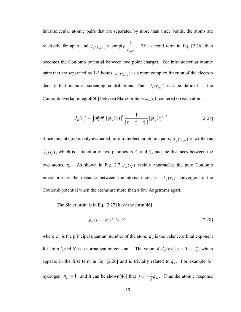
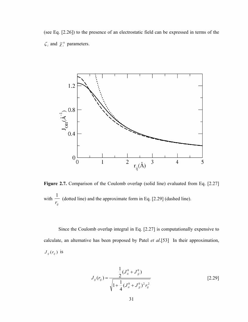
Figure 2.7. Comparison of the Coulomb overlap (solid line) evaluated from Eq. [2.27]

with ijr1

(dotted line) and the approximate form in Eq. [2.29] (dashed line). ................. 31 

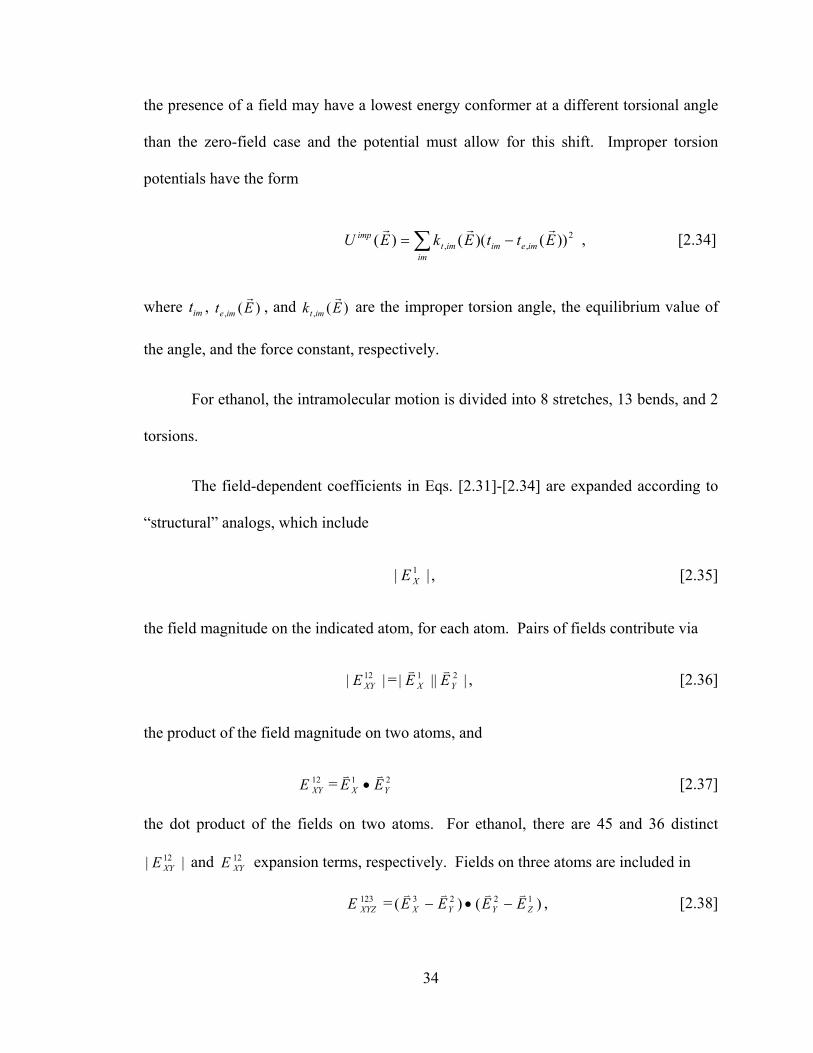
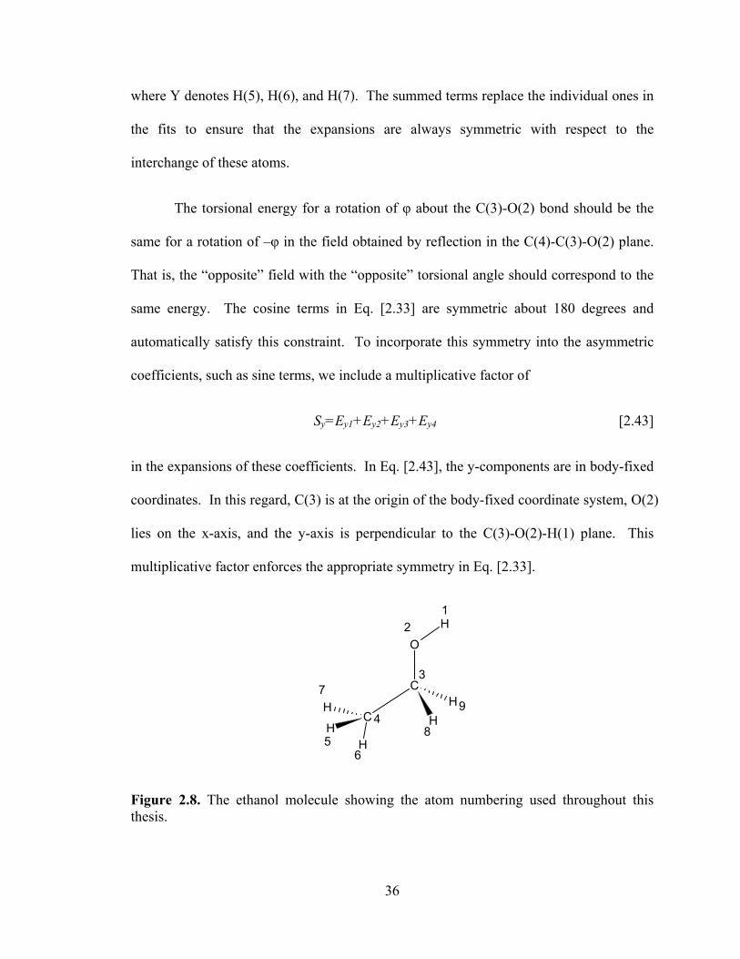
Figure 2.8. The ethanol molecule showing the atom numbering used throughout this thesis. ................................................................................................................................ 36 

Figure 2.9. The influence of torsional angles on chirality indexes of ethanol.. .............. 60 

Figure 2.10. Molecular structures and numbering system for (a) Whelk-O1, (b) DNB-leucine, (c) DNB-phenylglycine. ...................................................................................... 61 

Figure 3.1. Flow chart showing the seven steps involved in the design of the polarizable flexible ethanol model. ...................................................................................................... 68 

Figure 3.2. Statistics on the electric fields collected during the MD simulation using the flexible, non-polarizable Chen et al.[134] model of ethanol.. .......................................... 71 

xiii

Figure 3.3. The impact of the representation of the interatomic Coulomb interaction, )( ijij rJ . ............................................................................................................................. 76 

Figure 3.4. The torsional potential, )(EU torr

, between H(1)-O(2)-C(3)-C(4) as a function of the dihedral angle. .......................................................................................... 83 

Figure 3.5. The torsional potential, )(EU torr

, between O(2)-C(3)-C(4)-H(5) as a function of the dihedral angle. .......................................................................................... 85 

Figure 3.6. The impact of charge “mass” on the diffusion coefficient and radial distribution functions obtained from 20 ps simulations. ................................................... 89 

Figure 3.7. The energy components and the conserved quantity HNH as a function of time. .................................................................................................................................. 90 

Figure 3.8. The impact of damping on the range of parameter values allowed in the simulation. ......................................................................................................................... 92 

Figure 3.9. A comparison of radial distributions in bulk ethanol obtained from experiment, a non-polarizable model, and the fCINTRA polarizable model. .................. 94 

Figure 3.10. Snapshots of bulk ethanol from the fCINTRA polarizable, flexible model.......................................................................................................................................... 101 

Figure 4.1. The B3LYP/6-311++G(d,p) optimized structures for the solutes (a-c) and the solvents (d and e). ........................................................................................................... 109 

Figure 4.2. The barrier to rotation about the C(3)-O(2) bond of R-acenaphthenol as evaluated from B3LYP/6-31G(d) calculations ............................................................... 113 

Figure 4.3. The influence of torsional angles on chirality indexes of benzyl alcohol .. 115 

Figure 4.4. The coordinate system used to evaluate chirality indexes for solvent, illustrated for S-PAMD ................................................................................................... 116 

Figure 4.5. Convergence tests for excess chirality. ....................................................... 122 

Figure 4.6. Structure of ethanol and benzyl alcohol in the bulk and around the solutes.......................................................................................................................................... 127 

xiv

Figure 4.7. The impact of solvent polarizability on chirality transfer: The angle-dependence of ϕθ ,0 >< q

SG for ethanol hydrogen-bonded to the oxygen of S-PAMD. ... 131 

Figure 4.8. The impact of solute flexibility on chirality transfer. ................................. 134 

Figure 4.9. Impact of solutes on chirality transferred into hydrogen-bonding ethanol. ϕθ ,0 >< q

SG chiral indexes are shown along with illustrative snapshots. ........................ 141 

Figure 4.10. Impact of solutes on chirality transferred into hydrogen-bonding benzyl alcohol ............................................................................................................................. 142 

Figure 5.1. The influence of torsional angles on chirality indexes of 2-propanol. ....... 153 

Figure 5.2. The cylindrical coordinate system used in the spatial breakdown of excess chirality, average atomic charges, and average solvent dipole. ...................................... 155 

Figure 5.3. 2D solvent-selector distributions for potential H-bonding pairs at the Whelk-O1 interface. The position variables, z and r, are given in Å. ........................................ 161 

Figure 5.4. 2D distributions from 2-propanol/n-hexane solvated DNB-phenylglycine and DNB-leucine interfaces. .................................................................................................. 164 

Figure 5.5. An illustration of the convergence statistics for excess chirality.. ............. 166 

Figure 5.6. 2D distributions of average chirality indexes from the 2-propanol/n-hexane solvated DNB-leucine interface ...................................................................................... 169 

Figure 5.7. 2D distributions of average chirality indexes from the 2-propanol/n-hexane solvated DNB-phenylglycine interface. .......................................................................... 173 

Figure 5.8. 2D distributions of average chirality indexes from the 2-propanol/n-hexane solvated Whelk-O1 interface. ......................................................................................... 174 

Figure 5.9. Polarization of 2-propanol at the 2-propanol/n-hexane solvated DNB-leucine interface. .......................................................................................................................... 177 

Figure 5.10. 2D distributions of charges and average chirality indexes from the ethanol/n-hexane, ethanol, 2-propanol/n-hexane and 2-propanol solvated Whelk-O1 interface. .......................................................................................................................... 181 

xv

List of Abbreviations 2D 2-Dimensional

3D 3-Dimensional

AO Atomic Orbital

CD Circular Dichroism

CGTF Contracted Gaussian-Type Function

CHARMM Chemistry at HARvard Molecular Mechanics

CHELPG Charges from Electrostatic Potentials using a Grid based method

CI Configuration Interaction

CI95 95% Confidence Interval

CN Coordination Numbers

CSP Chiral Stationary Phase

DFT Density Functional Theory

DNB Dinitrobenzoyl

FC Fluctuating Charge

fCINTRA Fluctuating Charge and INTRAmolecular potential

FDA Food and Drug Administration

GTF Gaussian-Type Function

HPLC High-Performance Liquid Chromatography

LJ Lennard-Jones

MC Monte Carlo

MD Molecular Dynamics

MEP Molecular Electrostatic Potential

xvi

MP2 2nd order Moller-Plesset perturbation theory

MPI Message-Passing Interface

OPLS Optimized Potential for Liquid Simulations

ORD Optical Rotatory Dispersion

PAMD n-(1-(4-bromophenyl)ethyl)pivalamide

PBC Periodic Boundary Conditions

PIPF Polarizable Intermolecular Potential Function

PP Peak Position

PPC Polarizable Point-Charge

RU Rigid Unit

STO Slater Type Orbital

UA United Atom

VCD Vibrational Circular Dichroism

1

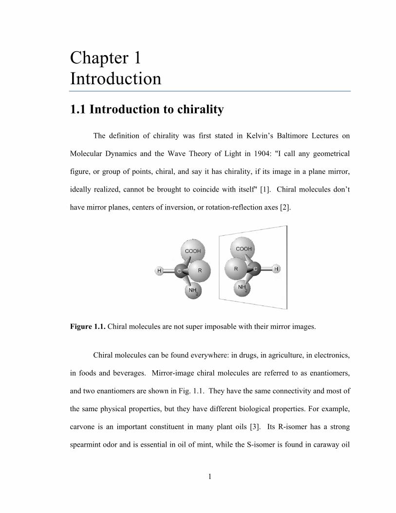
Chapter 1 Introduction 1.1 Introduction to chirality

The definition of chirality was first stated in Kelvin’s Baltimore Lectures on

Molecular Dynamics and the Wave Theory of Light in 1904: "I call any geometrical

figure, or group of points, chiral, and say it has chirality, if its image in a plane mirror,

ideally realized, cannot be brought to coincide with itself" [1]. Chiral molecules don’t

have mirror planes, centers of inversion, or rotation-reflection axes [2].

Figure 1.1. Chiral molecules are not super imposable with their mirror images.

Chiral molecules can be found everywhere: in drugs, in agriculture, in electronics,

in foods and beverages. Mirror-image chiral molecules are referred to as enantiomers,

and two enantiomers are shown in Fig. 1.1. They have the same connectivity and most of

the same physical properties, but they have different biological properties. For example,

carvone is an important constituent in many plant oils [3]. Its R-isomer has a strong

spearmint odor and is essential in oil of mint, while the S-isomer is found in caraway oil

2

and has a different odor [4]. Similarly, lemon and orange peels both contain limonene.

The S-enantiomer and R-enantiomer are found in lemon and orange peels, respectively,

and they have different odors [4]. These enantiomers have different scents because of the

different interactions between these molecules and our olfactory chiral receptors [5]. In a

more extreme case, thalidomide, which was a sedative drug in the late 1950s, caused a

tragedy because one enantiomer helped against nausea, while the other caused fetal

damage [6]. In 1992, the United States Food and Drug Administration (FDA) released a

new policy on chiral drugs, stating that all new drugs would need to be characterized

pharmacologically and toxicologically if they are to be marketed as racemic mixtures [7].

As a result of this new policy, the demand for chemical processes that can selectively

produce chiral molecules has greatly increased. In 1985, most chiral medicines were sold

as racemic mixtures [8]. In 1999, single-isomer chiral drugs accounted for only 32% of

the $360 billion pharmaceutical sales [9]. In 2006, in contrast, 75% of new drugs

approved by the FDA were single enantiomers [10].

The separation of chiral molecules is often difficult. Chiral pool and chiral

resolution are the most widely applied methods in industry [11]. The chiral pool consists

of naturally occurring chiral molecules that are enantiomerically pure, such as amino

acids, carbohydrates, hydroxy acids, alkaloids and terpenes. It is a very effective way of

introducing asymmetry into synthesis and keeping the chirality intact. In the early 1990s,

chiral pool materials were used to derive most of the chiral drugs [10]. However, chiral

pool synthesis relies heavily on catalysis, which makes it very time consuming,

unpredictable and costly [10].

3

Chromatographic techniques for separation of enantiomers have been developing

quickly in the past years. The chromatographic separation of enantiomers can be

achieved by various methods, but chiral discriminators or selectors are always needed.

There are two types of selectors that can be used: Chiral mobile phase additives and

chiral stationary phases (CSP) [12]. In the first case, enantioselective retention is caused

by the differences in adsorption properties of the formed diastereomeric complexes to an

achiral stationary phase [13, 14]. The chiral selection by CSP is due to differences in the

two stereo isomeric complexes that are formed between the enantiomers and the

selector [15].

1.2 Studies on chirality transfer

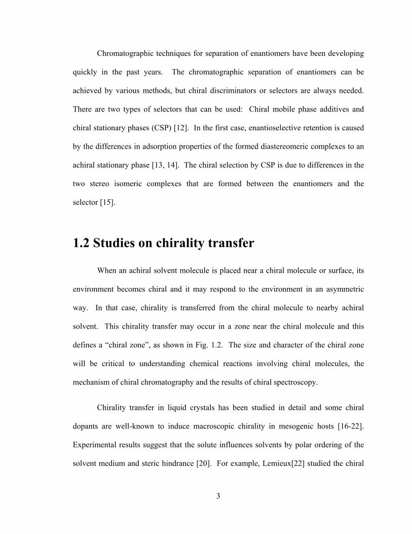
When an achiral solvent molecule is placed near a chiral molecule or surface, its

environment becomes chiral and it may respond to the environment in an asymmetric

way. In that case, chirality is transferred from the chiral molecule to nearby achiral

solvent. This chirality transfer may occur in a zone near the chiral molecule and this

defines a “chiral zone”, as shown in Fig. 1.2. The size and character of the chiral zone

will be critical to understanding chemical reactions involving chiral molecules, the

mechanism of chiral chromatography and the results of chiral spectroscopy.

Chirality transfer in liquid crystals has been studied in detail and some chiral

dopants are well-known to induce macroscopic chirality in mesogenic hosts [16-22].

Experimental results suggest that the solute influences solvents by polar ordering of the

solvent medium and steric hindrance [20]. For example, Lemieux[22] studied the chiral

4

induction in a smectic liquid crystal phase when doped with molecules with

atropisomeric biphenyl cores. It was found that the chirality transferred from chiral

dopants heavily depended on the core structure of the liquid crystal host and the

mechanism of the chirality transfer was explained by the concepts of host-guest

chemistry. Most of the current theoretical studies of this chirality transfer focus on the

correlation of solute properties with the experimentally measured helical twisting

power[23].

Figure 1.2. Representation of chiral “zones”. The left and right panels illustrate the chiral zone idea around a chiral solute and between chiral surfaces, respectively.

Compared to studies of chirality transfer in liquid crystals, isotropic phases are

relatively unexplored. However, it is known that solvent effects can greatly influence

spectroscopy, such as optical rotatory dispersion (ORD). Solvents can influence the

structures of solutes and indirectly affect the spectroscopy. For instance, Kumata et

al.[24] measured ORD spectra for S-methyloxirane, which is a small and relatively rigid

5

molecule with a three-membered ring, and observed a significant difference between its

optical rotation in water and in benzene. Fischer et al.[25] measured the optical rotation

of (S)-methylbenzylamine in a wide range of solvents with various concentrations, and

very large variations were observed. After comparing the experimental and calculated

results, they concluded that hydrogen bonding has large contributions on specific rotation.

Recently, experimental and theoretical studies have begun to focus on the

chirality induced in achiral solvent when it surrounds a chiral solute. Yashima et al.[26]

mentioned, in an NMR study, that the two methyl groups in 2-propanol were not

equivalent when they were in the proximity of cellulose tris(4-

trimethylsilylphenylcarbamate). Jennings[27] has reviewed the effect of chiral lanthanide

shift reagents, such as the tris[3-trifluoromethylhydroxymethylene-d-

camphorato]europium(III), on achiral solvents where the appearance of chemical shift

nonequivalence was observed in methyl groups of 2-propanol, 2-propylamine and 2-

methyl-2-butanol, and the methylene protons in 2,2-dimethylpropanol and 2-methyl-2-

butanol. In a recent vibrational circular dichroism(VCD) study, Losada et al.[28] found

evidence for chirality transfer from methyl lactate to hydrogen-bonded water. It was

found that the H–O–H bending modes of the achiral water molecules that are H-bonded

to a methyl lactate molecule gave rise to a strong VCD peak. This was further supported

by a series of density functional theory (DFT) calculations of methyl lactate-(H2O)n

complexes and it was concluded that the transfer involved one primary solvent molecule.

In contrast, Mukhopadhyay et al.[29, 30] suggested that solvent imprinting was a major

component of the ORD of methyloxirane in benzene and water. The authors used Monte

Carlo (MC) simulations combined with DFT methods and explicit solvent models and

6

found that the chiral distribution of the solvent molecules exceeded the contribution of

the solute itself. They also mentioned that an explicit solvent model was essential in

describing the chiroptical properties of molecules in solution. Fidler et al.[31] used MD

simulations to study the distribution of simple achiral solvent molecules surrounding a

chiral solute, and found that achiral solvents can contribute 10-20% of the circular

dichroism (CD) intensity. This implies that chirality has been induced in the solvation

shell. It was also found that the magnitude of the solvent effect depended strongly on the

nature of both the solute and the solvent.

These studies clearly confirm the presence of chirality transfer in solutions. This

effect can be important in organic reactions that employ chiral reagents and achiral

solvents because the induced chirality in solvents can have an impact on the reaction.

Alternatively, chiral chromatography uses binary or ternary achiral solvents in contact

with chiral surfaces. The induced chirality in the solvent hasn’t been considered in any of

the proposed selection mechanisms[15, 32-38], but, at least in principle, it could

influence the stereo selectivity if it is significant. Also, except for the examples

mentioned above, most of the current theoretical calculations of spectroscopy, such as

VCD and ORD, only consider the contributions from the chiral solutes and the solvent

effects on solutes, but the solvent molecules are always considered as internally achiral

and have no direct impact on the spectra. However, if the chirality transfer is strong

enough, the induced chirality in solvents may directly contribute to the spectra and,

therefore, can be important when trying to correctly interpret experimental results.

7

1.3 Polarizable models

Non-polarizable force fields for molecular simulations use effective pairwise

potentials for electrostatic interactions and are widely used in simulations of condensed

phases and biological systems [39, 40]. However, limitations exist in non-polarizable

force fields [39]. Because they use fixed atomic charges and intramolecular potentials,

which cannot adjust themselves according to different environments, the molecules are

not treated accurately. For instance, solvation free energy calculations indicate that these

force fields tend to underestimate the solubility of amino acid side chain analogs [41]. In

other studies, non-polarizable flexible models have been found to underestimate the

dipole moment of water molecules in bulk [42].

There is no doubt that simulation reliability depends upon the accuracy of the

potential functions. In order to study chirality transfer, potential functions should be very

sensitive to environmental changes so that asymmetric effects can be reflected.

Therefore, non-polarizable models are not sufficient for chirality transfer, and addition of

polarizability into the models is necessary.

There have been continuing efforts to incorporate polarization effects into non-

polarizable force fields [43-47]. More specifically, molecule’s mean response to a field

is taken into account by iterative schemes: The charges or dipole moments of molecules

can generate fields and the fields will, in turn, influence the charges or dipole moments of

each molecule. Gao et al.[43] developed a polarizable intermolecular potential function

(PIPF) for liquid alcohols. In this model, all atoms are represented explicitly, and the

total energy of the system consists of a pairwise term and a nonadditive polarization term.

The pairwise term is classical and is also used in non-polarizable models. The

8

polarization term follows from interactions between induced atomic dipole moments ( iμ )

and the electrostatic field at the position of each atom ( 0iE ):

∑−=N

iii

pol EE 0

21 μ [1.1]

The induced dipole moment is defined as

∑≠

⋅−=ij

jijiii TE )( 0 μαμ [1.2]

where iα is the polarizability and ijT is the dipole tensor. The induced dipole moments

are calculated self-consistently and 4-5 iterations are typically needed [43]. This model

provides a more accurate calculation of intermolecular interactions for heterogeneous

systems compared to non-polarizable models. The disadvantage of this model is obvious:

Self-consistency requires iterations at each time step, which makes it much more time

consuming than non-polarizable models. More importantly, the atomic dipole moment is

only conceptual and cannot provide information on real properties such as charge

distributions.

Noskov et al.[42, 44, 45, 48] include charge carrying Drude particles in their

molecular model to allow the molecular dipole to respond to the field. This model,

originally proposed by Paul Drude in 1900[49], redistributes the partial charge on a

heavy atom, such as oxygen, among a set of massless charged sites connected by a

harmonic spring. The positions of these auxiliary sites are self-consistently determined in

response to the external field, and the charges and force constants of these fictitious

particles are related to the atomic polarizability. Before using the Drude model, the

number and distribution of these auxiliary sites should be chosen. This model has been

9

used to successfully reproduce the vaporization enthalpy, dielectric constant, and self-

diffusion of bulk liquids, such as water and ethanol. Similar to the PIPF, this model is

computationally expensive because for each simulation step, about 16 iterations are

required by the self-consistent procedure [42, 44].

Svishchev et al.[47] developed a polarizable point-charge (PPC) model for water.

This three-site water model introduced field-dependence to atomic charges and

intramolecular structures. In the implementation of this model, the atomic charges are

iterated to calculate the self-consistent electrostatic fields and three to four iterations are

normally required in each time step. This model has been used to successfully reproduce

the static and dynamics properties of liquid water from supercooled to near-critical

conditions[47].

Rick et al.[46], building upon earlier work by Rappé and Goddard[50], introduced

a fluctuating charge (FC) model that uses an extended Hamiltonian approach to allow the

molecules to respond to their environment. Specifically, this model was derived on the

basis of the principle of electronegativity equalization[50], and starts with the energetic

costs of charging an atom. The atomic charges are assigned fictitious masses and the

charge values are dynamic variables. The charge fluctuations are dependent on the

electrostatic field and subjected to the overall charge constraint, such as charge neutrality

for each molecule. This model has been used by a number of groups[51-55] to study

condensed phases as well as biological systems, such as peptides, and favorable results

have been reported. For instance, average molecular dipole moments predicted by the FC

model were found to be higher than those in non-polarizable models and closer to

experiments even though the starting dipole moments are consistent with those in the gas

10

phase [54]. Unlike other polarizable models, the FC model doesn’t require any iteration

to achieve self-consistency since it is an extended Hamiltonian approach. This makes the

cost of the simulation only slightly more than for a non-polarizable model. The

disadvantage of this model is that, due to the fast fluctuations of atomic charges, the time

step in the simulations is smaller in order to remain on the Born-Oppenheimer surface. A

way to improve this is to propagate charge degrees of freedom separately from the

nuclear degrees of freedom [56].

Although these models incorporate polarization effects by making electrostatic

potentials field-dependent, they all treat the intramolecular potentials to be stationary.

However, when molecules are in different environments, their intramolecular potentials,

such as the torsional potentials, could be different. A field-dependent intramolecular

potential has been developed only once previously, for water [57]. In that model, the HH

and OH stretching potentials depended on the field magnitude of oxygen. However, this

model is specific to water and the atomic charges were field-independent. Therefore,

prior to the current work, a polarizable model that includes field dependence in both the

atomic charges and the intramolecular degrees of freedom had not been considered.

In all, polarizable models can accurately describe a molecule’s responses to

different environments and hence, can increase the accuracy of MD simulations. Both

the atomic charges and intramolecular potentials should be polarizable in order to

accurately capture rapid changing properties, such as the induced chirality. However,

none of the existing methods incorporates all these features. Therefore, a new

methodology for developing this polarizable model is needed. The development and

implementation of a flexible, polarizable model is discussed in Chapter 3.

11

1.4 Measuring chirality

The usual way to experimentally measure chirality is to use spectroscopy, such as

CD, ORD and VCD [58-60]. These techniques are usually restricted to bulk samples. In

a recent study of fluorescence-detected circular dichroism, Hassey et al.[61] analyzed

dissymmetry parameters of single (bridged triarylamine) helicene molecules, and found

that both relatively large positive and negative dissymmetry parameters could be

observed although the measured spectra of bulk samples only have very small positive or

negative values because of cancellation effects.

The chirality of individual molecules can be quantified by chirality indexes,

which have been a subject of continuing interest over the past fifteen years, as

summarized in several reviews[62, 63]. Many chiral indexes have been proposed[62, 64-

69], but most of them can be divided into two general classes: measures that quantify the

difference between a chiral object and an achiral reference[68], and those that quantify

the difference between an enantiomer and its mirror image[69].

The first chirality function in chemistry was proposed by Guye et al.[70] in 1890.

They introduced a function that correlated the optical rotation, which is a pseudoscalar

property, with the molecular structure of a chiral molecule [62]. According to Guye, if

the masses of the four points in a tetrahedral model are set to be the same, the chirality

index P for a tetrahedron can be defined by ∏>

−=4

)()(ji

ji llclP , where jl is the distance

between the four vertices. In this definition, )(lP is only a function of geometry and is

non-zero only in the asymmetric tetrahedron. Therefore, this index indicates the

distortion of a simple tetrahedron from its achiral form. Murrayrust et al.[71, 72]

12

improved this chirality function and represented the atomic configuration of a molecule

by a point in a multidimensional space. The deformation of the configuration away from

the symmetric reference structure can be calculated from the distance from this point to

the axis.

In the chiral indexes that quantify the difference between two enantiomers, the

common volumes and Hausdorff Distances are the most famous [68, 69]. Let’s still take

the tetrahedron as an example. When overlapping the tetrahedron with its mirror image,

there’s a volume that is occupied by both of them. When you rotate one tetrahedron

around and get the maximum overlapping volume, that volume is the common volume.

When a tetrahedron is achiral, the common volume is equal to the molecular volume.

Therefore, this property can be used as a chiral index. A Hausdorff Distance measures

how far two subsets of a space are from each other and is defined as:

)},(infsup),,(infsupmax{ yxdyxdDXxYyYyXx

H ∈∈∈∈= [1.3]

where sup and inf are supremum and infimum, respectively, and d(x,y) is the distance of

two points x and y. Fig. 1.3 illustrates the concept of Hausdorff Distance. The nuclear

positions in a rigid molecular model can be represented by a subset of points in three-

dimensional space, and the Hausdorff Distance between the original and achiral point sets,

indicates the measure of chirality.

13

Figure 1.3. The Hausdorff Distance. The set X and Y correspond to all points inside the rectangle and the ellipse, respectively. ),(infsup yxd

YyXx ∈∈ is the maximum distance from any

points in X (rectangle) to the closest point in Y (ellipse). ),(infsup yxdXxYy ∈∈

is the maximum

distance from any points in Y to the closest point in X. The Hausdorff Distance is the maximum of the two.

More recently, Osipov et al.[66] proposed a new chirality index that is different

from the previous ones. It does not rely on a comparison to an achiral reference or a

mirror image. This chirality index is analogous to the optical activity tensor[66], and has

been found to accurately predict the helical twisting power of chiral dopants[73-76] for

relatively rigid twisted-core additives. For more flexible additives, the relationship

between the chiral index and the twisting power reflected conformational preferences due

to interaction with the liquid crystal host[76, 77].

Although chirality indexes are supposed to be non-zero when a molecule is chiral,

it has been found that if a chirality index is continuous, there almost always exist chiral

zeroes [78]. The rationale for this is based on the following arguments. It is assumed

that a molecular structure belongs to a continuous set, and any two structures can be

connected by a continuous conversion. Except for some rare cases[79, 80], a chiral

14

molecule can be converted into its mirror image along a chiral path and all structures on

this path are chiral. Since the chirality indexes of the two enantiomers have the same

magnitude and opposite signs, there must be at least a point, during the conversion, that

the chirality index becomes zero but the molecular structure is still chiral. In fact, there

are an infinite number of such points for any molecule. Therefore, special care should be

taken to deal with chiral zeroes when selecting chirality indexes.

There are several challenges to assess chirality in molecular dynamics simulations.

First, within the simulations, all the molecules are flexible and mobile. The assessed

chirality must reflect the conformational changes of each molecule but stay constant for

reorientation or translation. Second, achiral molecules will be instantaneously chiral but,

over long times, this chirality should average to zero when the molecules are far from a

source of chirality. Third, the evaluation of instantaneous chirality must be rapid enough

to allow simulations to proceed.

In order to study chirality transfer, it is important to choose proper chirality

indexes. The indexes developed by Osipov et al[66] are chosen in our study because

they fit all our requirements and can be modified to emphasize molecular shape, atomic

charges, or atomic masses, etc.. By using multiple indexes, we can focus on different

aspects of the molecular structures and charge distributions and prevent chiral zeroes at

the same time.

15

1.5 Thesis organization

The main objective of this thesis is to explore the chirality transfer from chiral

solutes and surfaces to achiral solvents. To achieve this goal, a new methodology for

building polarizable, flexible models is developed.

This thesis is organized as follows. Chapter 2 presents theoretical methods,

simulation algorithms, and details on polarizable models and chirality indexes. Chapter 3

describes the development of polarizable and flexible molecular models based on

extensive ab initio calculations. In this methodology, intramolecular motion is directly

coupled to electrostatic fields. Chapter 4 presents MD simulation results on chirality

transfer from chiral solutes to achiral solvents, such as ethanol and benzyl alcohol.

Detailed aspects such as the importance of solvent polarizability and solute flexibility,

hydrogen-bonding network, and the solvent-solute interaction sites are described.

Chapter 5 presents results on chiral induction studies for surfaces used in chiral

chromatography, such as the Whelk-O1, leucine- and phenylglycine-based CSPs. The

solvents consist of ethanol, 2-propanol, and binary solvents that are commonly used in

chromatography, such as n-hexane/ethanol and n-hexane/2-propanol. Emphasis is placed

on the location of the chirality transfer zones and the solvent characteristics in these

zones. Brief conclusions are presented in Chapter 6.

16

Chapter 2 Theoretical Methods and Models 2.1 Molecular dynamics simulations

Most of the results in this thesis are obtained from Molecular Dynamics (MD)

simulations. The MD simulation technique is used to calculate equilibrium and

dynamical properties of many-body systems. It has been used widely from ideal gases

and liquids to biomolecules[40, 81]. For every particle in the system, the forces acting

upon it are calculated and Newton’s equations are used to evolve the system. In the

simulations, the coordinates and momenta of all particles are obtained and the physical

properties can be calculated using statistical mechanics methods. Therefore, MD is a

bridge between theoretical and experimental approaches: It is a computer-based

experiment. MD simulation is particularly useful for systems that are too difficult to be

studied experimentally or too complicated to be studied by quantum mechanical

approaches.

In a classical system of N molecules, the Hamiltonian ),( pqH rr is the sum of

kinetic and potential energies and is a function of the coordinates ),...,,( 21 Nqqqq rrrr= and

momenta ),...,,( 21 Npppp rrrr= of each atom:

)()(),( qUpKpqH rrrr+= [2.1]

where )(pK r and )(qU r

are kinetic and potential energies, respectively. The kinetic

energy has the form

17

∑∑=N M

i i

i

mppK

α α

α

2)(

2r [2.2]

where N and M are the number molecules and the number of atoms in each molecule,

respectively, and αim is the atomic mass of atom i in molecule α . From the Hamiltonian,

the equations of motion can be derived:

α

α

α

α

i

i

i

i

mp

pH

dtqd r

r

r

=∂∂

= [2.3]

αα

α

ii

i

qU

qH

dtpd

rr

r

∂∂

−=∂∂

−= [2.4]

Eq. [2.4] can also be written as the total force acting on atom i of molecule α :

ααα

αα

α iii

ii

i amdt

qdmqUF r

r

rr

==∂∂

−= 2

2

[2.5]

In MD simulations, forces are calculated in each time step and the equations of motions

are solved to advance the system in time. Therefore, the force calculation is essential to

MD simulations.

2.1.1 Potentials

As shown in Eq. [2.5], forces are obtained from first derivatives of the potential

( )(qU r). Generally, the total potential is divided into two parts: An intramolecular part

and an intermolecular part:

interintra UUU += [2.6]

18

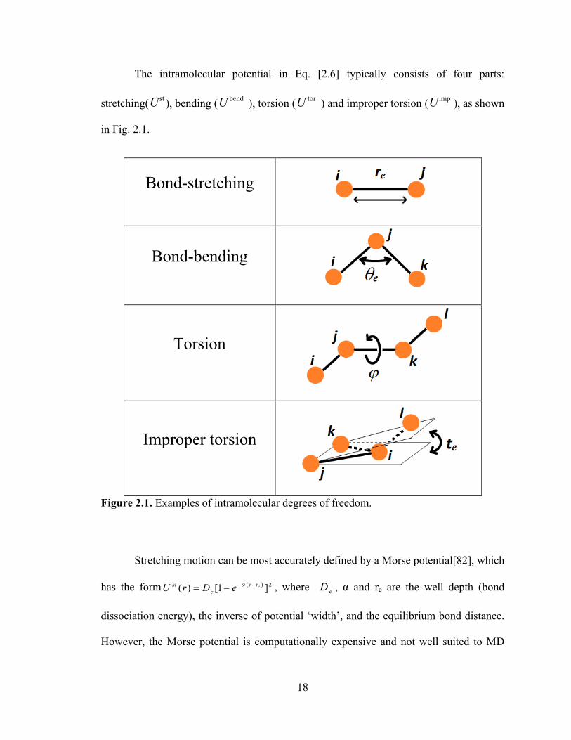
The intramolecular potential in Eq. [2.6] typically consists of four parts:

stretching( stU ), bending ( bendU ), torsion ( torU ) and improper torsion ( impU ), as shown

in Fig. 2.1.

Bond-stretching

Bond-bending

Torsion

Improper torsion

Figure 2.1. Examples of intramolecular degrees of freedom.

Stretching motion can be most accurately defined by a Morse potential[82], which

has the form 2)( ]1[)( erre

st eDrU −−−= α , where eD , α and re are the well depth (bond

dissociation energy), the inverse of potential ‘width’, and the equilibrium bond distance.

However, the Morse potential is computationally expensive and not well suited to MD

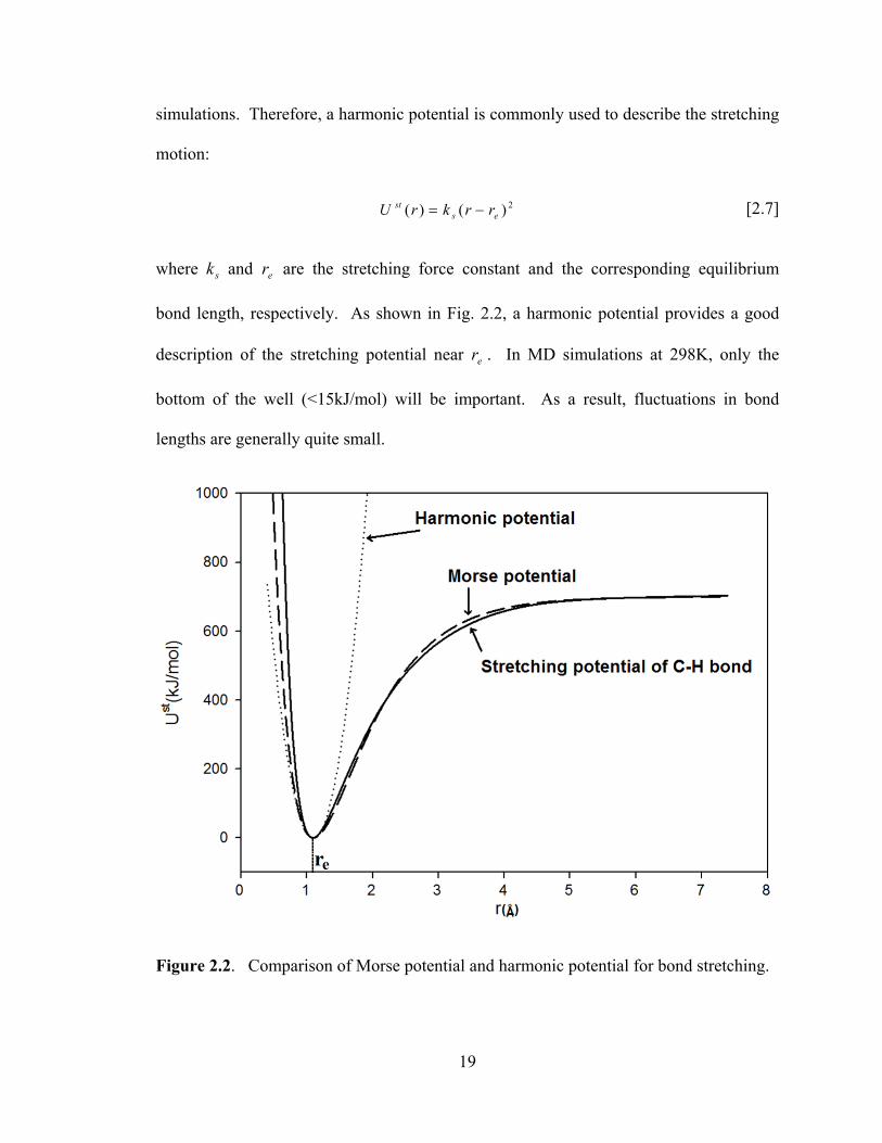
19

simulations. Therefore, a harmonic potential is commonly used to describe the stretching

motion:

2)()( esst rrkrU −=

[2.7]

where sk and er are the stretching force constant and the corresponding equilibrium

bond length, respectively. As shown in Fig. 2.2, a harmonic potential provides a good

description of the stretching potential near er . In MD simulations at 298K, only the

bottom of the well (<15kJ/mol) will be important. As a result, fluctuations in bond

lengths are generally quite small.

Figure 2.2. Comparison of Morse potential and harmonic potential for bond stretching.

20

Typical MD simulations keep bond lengths fixed by using the RATTLE[83] or

SHAKE[84] algorithms, and a bond stretching potential is only used for some selected

bonds.

Bending can also be defined by a harmonic potential,

2bend )()( ekU θθθ θ −= [2.8]

where θk and eθ are the bending force constant and the corresponding equilibrium angle,

respectively. Other more complicated forms have been employed, but, as with bond

stretches, bending motion is limited at typical temperatures and a harmonic potential is

usually sufficient.

The torsion potential has the form of a modified Ryckaert-Bellemans potential[85]

[2.9]

where iC is the ith torsional coefficient, ϕ is the dihedral angle and iϕ is the

corresponding phase shift. Other forms of torsion potentials are also available[86] and

will not be discussed here.

Improper torsion potentials have the form

2)()( etimp ttktU −=

[2.10]

where t, te, and kt are the improper torsion angle, the equilibrium value of the angle, and

the force constant, respectively.

The intermolecular potential in Eq. [2.6] can be written as

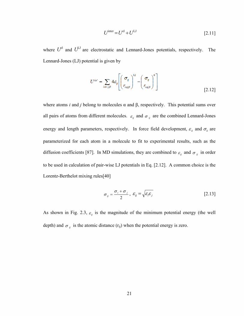
21

LJelinter UUU += [2.11]

where elU and LJU are electrostatic and Lennard-Jones potentials, respectively. The

Lennard-Jones (LJ) potential is given by

[2.12]

where atoms i and j belong to molecules α and β, respectively. This potential sums over

all pairs of atoms from different molecules. ijε and ijσ are the combined Lennard-Jones

energy and length parameters, respectively. In force field development, iiε and iiσ are

parameterized for each atom in a molecule to fit to experimental results, such as the

diffusion coefficients [87]. In MD simulations, they are combined to ijε and ijσ in order

to be used in calculation of pair-wise LJ potentials in Eq. [2.12]. A common choice is the

Lorentz-Berthelot mixing rules[40]

2ji

ij

σσσ

+= , jiij εεε = [2.13]

As shown in Fig. 2.3, ijε is the magnitude of the minimum potential energy (the well

depth) and ijσ is the atomic distance (rij) when the potential energy is zero.

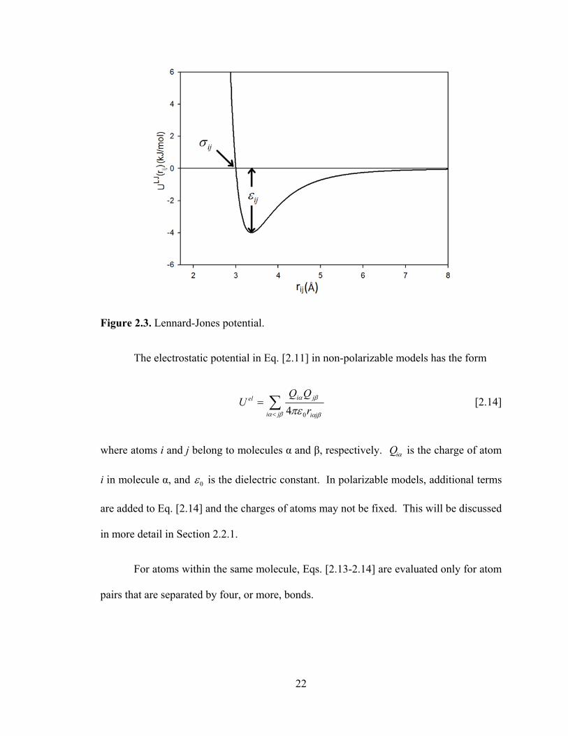
22

Figure 2.3. Lennard-Jones potential.

The electrostatic potential in Eq. [2.11] in non-polarizable models has the form

∑<

=βα βα

βα

πεji ji

jiel

rQQ

U04

[2.14]

where atoms i and j belong to molecules α and β, respectively. αiQ is the charge of atom

i in molecule α, and 0ε is the dielectric constant. In polarizable models, additional terms

are added to Eq. [2.14] and the charges of atoms may not be fixed. This will be discussed

in more detail in Section 2.2.1.

For atoms within the same molecule, Eqs. [2.13-2.14] are evaluated only for atom

pairs that are separated by four, or more, bonds.

23

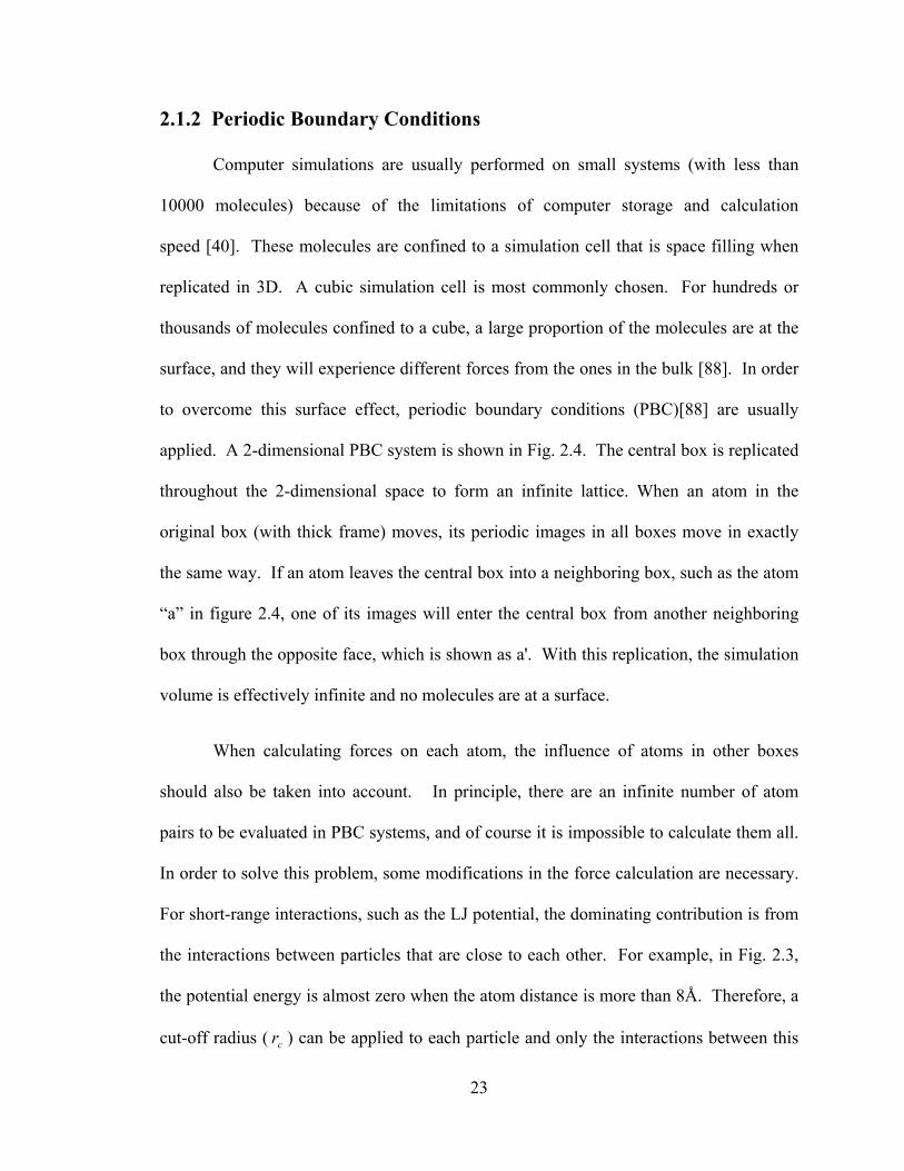
2.1.2 Periodic Boundary Conditions

Computer simulations are usually performed on small systems (with less than

10000 molecules) because of the limitations of computer storage and calculation

speed [40]. These molecules are confined to a simulation cell that is space filling when

replicated in 3D. A cubic simulation cell is most commonly chosen. For hundreds or

thousands of molecules confined to a cube, a large proportion of the molecules are at the

surface, and they will experience different forces from the ones in the bulk [88]. In order

to overcome this surface effect, periodic boundary conditions (PBC)[88] are usually

applied. A 2-dimensional PBC system is shown in Fig. 2.4. The central box is replicated

throughout the 2-dimensional space to form an infinite lattice. When an atom in the

original box (with thick frame) moves, its periodic images in all boxes move in exactly

the same way. If an atom leaves the central box into a neighboring box, such as the atom

“a” in figure 2.4, one of its images will enter the central box from another neighboring

box through the opposite face, which is shown as a'. With this replication, the simulation

volume is effectively infinite and no molecules are at a surface.

When calculating forces on each atom, the influence of atoms in other boxes

should also be taken into account. In principle, there are an infinite number of atom

pairs to be evaluated in PBC systems, and of course it is impossible to calculate them all.

In order to solve this problem, some modifications in the force calculation are necessary.

For short-range interactions, such as the LJ potential, the dominating contribution is from

the interactions between particles that are close to each other. For example, in Fig. 2.3,

the potential energy is almost zero when the atom distance is more than 8Å. Therefore, a

cut-off radius ( cr ) can be applied to each particle and only the interactions between this

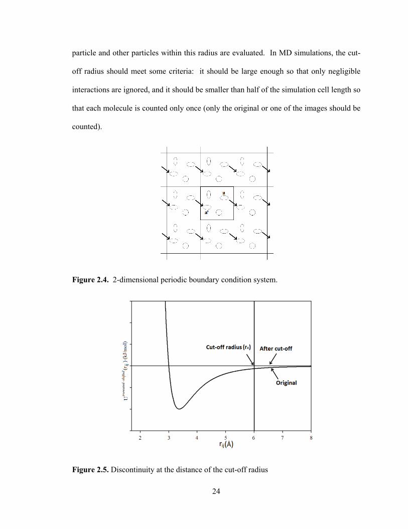
24

particle and other particles within this radius are evaluated. In MD simulations, the cut-

off radius should meet some criteria: it should be large enough so that only negligible

interactions are ignored, and it should be smaller than half of the simulation cell length so

that each molecule is counted only once (only the original or one of the images should be

counted).

Figure 2.4. 2-dimensional periodic boundary condition system.

Figure 2.5. Discontinuity at the distance of the cut-off radius

25

Applying a cut-off radius will introduce a discontinuity at the distance of cr , as

shown in Fig. 2.5. Since forces are obtained from derivatives of the potential, the

discontinuity in the potential can cause an infinite force at cr . The potential is normally

shifted after truncation so that it becomes continuous:

)()()( cLJ

ijLJ

ijshiftedtruncated rUrUrU −=−

when cij rr ≤

0)( =−ij

shiftedtruncated rU when cij rr ≤ [2.15]

and the potential and force vary smoothly with distance.

2.1.3 Ewald summation

In MD simulations, the evaluation of long-range interactions (charge-charge,

charge-dipole, dipole-dipole) is time consuming. In a cubic simulation cell of side

length L with N charged atoms, the Coulombic potential energy is:

∑=

Φ=N

iii

Coulomb rQU1

)(21 r

[2.16]

where iQ

and irr

are the partial charge and position of atom i, respectively, and )( irr

Φ

is

the electrostatic potential at the position of atom i.

∑∑= +

=ΦN

j n ij

ji Lnr

Qr

1 ||)(

rrr

r [2.17]

where ),,( zyx nnnn =r ,

with zyx nnn ,, integers, includes the positions of atoms in the

images. The summation omits the case of i=j, where )0,0,0(=nr since a charge does not

interact with itself. Here, atomic units are used to make the notation more compact.

26

Unlike LJ potentials, molecules in neighboring cells must be included in the evaluation of

)( irr

Φ , but the result of this summation depends on the order in which the terms are

added up, and thus a direct evaluation of )( irr

Φ suffers from convergence problems [81].

The Ewald summation[89] was introduced many years ago to effectively sum the

long-range interactions between an infinite number of particles and all their periodic

images. In this approach, each charge is considered to be surrounded by a screening

charge distribution (normally Gaussian distribution) of equal magnitude but of opposite

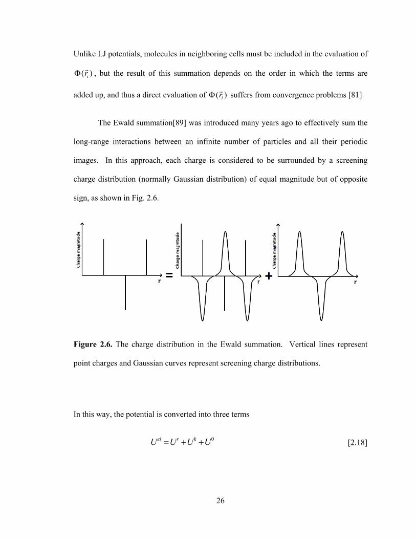
sign, as shown in Fig. 2.6.

Figure 2.6. The charge distribution in the Ewald summation. Vertical lines represent

point charges and Gaussian curves represent screening charge distributions.

In this way, the potential is converted into three terms

0UUUU krel ++= [2.18]

27

The first term, rU , is the sum of the interactions between the charges plus the

screening distributions, and it is a real space sum[89]:

∑∑≠ +

+=

N

ji n ij

ijji

r

LnrLnrerfc

QQUr

rr

rr

|||)|(

21 α

[2.19]

where α determines the size of the screening distribution and )(xerfc is the

complementary error function that decreases monotonically as x increases

∫∞

−=x

t dtexerfc22)(

π [2.20]

The second term in Eq. [2.18], kU , exactly counteracts the first screening

distribution, and this summation is performed in reciprocal space

)cos()4

exp(42

12

2

1, 023 ij

N

ji kji

k rkkk

QQL

U rr

r⋅−= ∑∑

= ≠ απ

π [2.21]

where )2,2

,2(Ln

Ln

Lnk zyx πππ

=r

with zyx nnn ,, integers.

The third term in Eq. [2.18], 0U , is a correction term that cancels out the

interaction of each of the introduced artificial counter-charges with itself.

∑=

−=N

iiQU

1

20

πα

[2.22]

Therefore, Eq. [2.18] can be written as:

28

)cos()4

exp(42

1||

|)|(21

2

2

1, 023 ij

N

ji kji

N

ji n ij

ijji

k rkkk

QQLLnr

LnrerfcQQU rr

rr

rr

rr⋅−+

++

= ∑∑∑∑= ≠≠ α

ππ

α

∑=

−N

iiQ

1

2

πα

[2.23]

where α and the number of kr

vectors in the second sum are configurable parameters and

they should be carefully chosen so that Eq. [2.23] converges quickly. In practice, α can

be chosen such that rU only requires the central simulation cell and no images are

needed.

In Eq. [2.23], it is assumed that the simulation cell is cubic. If the simulation cell

is not cubic, an additional shape-dependent correction term, ),( PMJr

, should be

added,[90] where Mr

is the dipole moment of the simulation cell and ∑=

=N

iiirQM

1

rr. This

correction term depends on the summations geometry and has the following form for the

rectangular shape cell elongated on the z axis:

22)( zMV

MJ π=

r [2.24]

where Mz and V are the z component of the total dipole moment and the volume of the

simulation cell, respectively.

29

2.2 Polarizable Models

2.2.1 Fluctuating Charge Model

In non-polarizable force fields, fixed atomic charges are used in the molecules.

Since the charges are constant, they cannot reflect the changes in electrostatic

environments experienced by the molecules during the simulation. Rick et al.[46],

introduced a fluctuating charge (FC) model that allows the molecules to respond to their

environment. In the FC model, the energy of an isolated charged atom, bearing a charge

iQ , can be expanded in a Taylor expansion up to second order:

200

21~)0()( iiiiiii QJQEQE ++= χ [2.25]

where )0(iE and 0~iχ are the ground state energy and the electronegativity per unit

charge of atom i, respectively, and 0iiJ is twice the hardness of the electronegativity of

the atom. The values of 0~iχ and 0

iiJ can be obtained from ab initio calculations, from

empirical forms, or from experiments.

Within the FC model, the electrostatic energy of a system of M molecules (with N

atoms per molecule) is:

[2.26]

where i is an atom in molecule α and j belongs to molecule β. The first term is the energy

for each isolated atom and the second term is the electrostatic energy between all pairs of

atoms, both intramolecular and intermolecular. For intermolecular atomic pairs or

30

intramolecular atomic pairs that are separated by more than three bonds, the atoms are

relatively far apart and )( βαjiij rJ is simply βαjir

1. The second term in Eq. [2.26] then

becomes the Coulomb potential between two point charges. For intramolecular atomic

pairs that are separated by 1-3 bonds, )( βαjiij rJ is a more complex function of the electron

density that includes screening contributions. The )( βαjiij rJ can be defined as the

Coulomb overlap integral[50] between Slater orbitals, )( ini rϕ , centered on each atom:

∫ −−= 22 |)(|

||1|)(|)( jnj

ijjiinijiijij r

rrrrrdrdrJ ϕϕ rrr

rr [2.27]

Since this integral is only evaluated for intramolecular atomic pairs, )( βαjiij rJ is written as

)( ijij rJ , which is a function of two parameters iζ and jζ and the distances between the

two atoms, ijr . As shown in Fig. 2.7, )( ijij rJ rapidly approaches the pure Coulomb

interaction as the distance between the atoms increases: )( ijij rJ converges to the

Coulomb potential when the atoms are more than a few Angstroms apart.

The Slater orbitals in Eq. [2.27] have the form[46]

rnini

ii erNr ζϕ −−= 1)( [2.28]

where in is the principal quantum number of the atom, iζ is the valence orbital exponent

for atom i, and Ni is a normalization constant. The value of )(rJ ii at r = 0 is 0iiJ , which

appears in the first term in Eq. [2.26] and is trivially related to iζ . For example for

hydrogen, 1=Hn , and it can be shown[46] that HHHJ ζ850 = . Thus the atomic response

31

(see Eq. [2.26]) to the presence of an electrostatic field can be expressed in terms of the

iζ and 0~iχ parameters.

Figure 2.7. Comparison of the Coulomb overlap (solid line) evaluated from Eq. [2.27]

with ijr1

(dotted line) and the approximate form in Eq. [2.29] (dashed line).

Since the Coulomb overlap integral in Eq. [2.27] is computationally expensive to

calculate, an alternative has been proposed by Patel et al.[53] In their approximation,

)( ijij rJ is

2200

00

)(411

)(21

)(

ijjjii

jjii

ijij

rJJ

JJrJ

++

+= [2.29]

32

and the requirement for numerical integration (Eq. [2.27]) is avoided.

In Fig. 2.7, the Coulomb overlap evaluated from Eq. [2.27] is compared with ijr1

(Coulomb potential) and the approximate form in Eq. [2.29]. The approximate form in

Eq. [2.29] leads to )( ijij rJ that are close to the values from Eq. [2.27]. However, it has

been found[91] that even small changes in the )( ijij rJ lead to large differences in the

fluid structure and properties. Therefore, the more accurate form (Eq. [2.27]) is used in

our studies. In order to prevent expensive on-the-fly calculations of Eq. [2.27] during the

simulations, we evaluate the overlap for 500 interatomic separations, ijr , from 0-5 Ǻ prior

to the simulation. During the simulations, the interatomic separations will not normally

coincide with a pre-calculated separation, and we employ spline fits to interpolate

between calculated potentials and provide the Coulomb overlap at the required separation.

The approximation is very accurate because of the large number of interatomic

separations that are pre-evaluated and the monotonically decreasing nature of )( ijij rJ .

2.2.2 Fluctuating Charge and INTRAmolecular potential model

The intramolecular potentials are typically parameterized prior to the simulations

and are kept fixed thereafter. However, the potentials could be field sensitive and may

change during simulations due to the varying electrostatic environments experienced by

the molecules. In this thesis, the development of a new model, the Fluctuating Charge

and INTRAmolecular potential (fCINTRA) model, is described. In this model, the

environmental effects on atomic charges and intramolecular potentials are taken into

33

account. We have chosen ethanol as a test molecule but note that the principles outlined

below are general.

The field-dependent intramolecular potential generally consists of four parts:

)()()()()(intra EUEUEUEUEU imptorbestrrrrr

+++= . [2.30]

where Er

is the electrostatic field, and )(EU str

, )(EU ber

, )(EU torr

, and )(EU impr

are the

field-dependent stretching, bending, torsion, and improper torsion potentials, respectively.

Similar to Eq. [2.7], stretching motion is described by a harmonic potential,

∑ −=is

iseisissst ErrEkEU 2

;; ))()(()(rrr

[2.31]

where )(; Ek iss

r is the field-dependent stretching force constant, and )(; Er ise

r is the

corresponding equilibrium bond length. The bending potential is also described by a

harmonic potential

∑ −=ib

ibeibibbe EEkEU 2

;; ))()(()(rrr

θθθ [2.32]

where )(; Ek ib

rθ is the field-dependent bending force constant, and )(; Eibe

rθ is the

corresponding equilibrium angle. The torsional potential has the form

∑ ∑ ⎟⎠

⎞⎜⎝

⎛ +==it i

ititi

iittor EECEU ))((cos)()(

6

0,0;

rrrϕϕ

[2.33]

where itϕ is the dihedral angle and )(,0 Eit

rϕ is the corresponding phase shift. The latter is

important in representing the field response of the molecule. Specifically, the potential in

34

the presence of a field may have a lowest energy conformer at a different torsional angle

than the zero-field case and the potential must allow for this shift. Improper torsion

potentials have the form

∑ −=im

imeimimtimp EttEkEU 2

,, ))()(()(rrr

,

[2.34]

where imt , )(, Et ime

r, and )(, Ek imt

r are the improper torsion angle, the equilibrium value of

the angle, and the force constant, respectively.

For ethanol, the intramolecular motion is divided into 8 stretches, 13 bends, and 2

torsions.

The field-dependent coefficients in Eqs. [2.31]-[2.34] are expanded according to

“structural” analogs, which include

|| 1XE , [2.35]

the field magnitude on the indicated atom, for each atom. Pairs of fields contribute via

|| 12XYE = |||| 21

YX EEvv

, [2.36]

the product of the field magnitude on two atoms, and

12XYE = 21

YX EEvv

• [2.37]

the dot product of the fields on two atoms. For ethanol, there are 45 and 36 distinct

|| 12XYE and 12

XYE expansion terms, respectively. Fields on three atoms are included in

123XYZE = )()( 1223

ZYYX EEEEvvvv

−•− , [2.38]

35

corresponding to a field “angle” term on the middle atom, and

123XYZE

)= )()( 1223

ZYYX EEEEvvvv

×•× , [2.39]

corresponding to a “dihedral angle” form of 123XYZE . For ethanol, all possible angles are

considered, leading to 13 123XYZE and 123

XYZE)

terms. Finally, we include

1234XYZAE = ))()(())()(( 12232334

XYYZYZZA EEEEEEEEvvvvvvvv

−×−•−×− , [2.40]

which is analogous to a dihedral angle. With all possible torsions considered, twelve

four-field terms are obtained for ethanol. The expansion terms in Eqs. [2.35]-[2.40] are

invariant to the coordinate system (body-fixed or space-fixed) and, consequently, can be

readily evaluated during the simulation without a coordinate transformation.

In principle, coefficients in Eqs. [2.31]-[2.34] can be expanded to many field-

dependent terms obtained from Eqs. [2.35]-[2.40]. Symmetry considerations can reduce

the number of expressions. Take ethanol as an example, following the numbering in Fig.

2.8, since H(8) and H(9) are related by symmetry, we define

XHOCHE 123 = 1238

HOCHE + 1239HOCHE [2.41]

where X is used to represent atoms 8 and 9. Equivalently, for H(5), H(6), and H(7), we

have sums of three terms:

YCCHE 34)

= 345CCHE)

+ 346CCHE)

+ 347CCHE)

[2.42]

36

where Y denotes H(5), H(6), and H(7). The summed terms replace the individual ones in

the fits to ensure that the expansions are always symmetric with respect to the

interchange of these atoms.

The torsional energy for a rotation of φ about the C(3)-O(2) bond should be the

same for a rotation of –φ in the field obtained by reflection in the C(4)-C(3)-O(2) plane.

That is, the “opposite” field with the “opposite” torsional angle should correspond to the

same energy. The cosine terms in Eq. [2.33] are symmetric about 180 degrees and

automatically satisfy this constraint. To incorporate this symmetry into the asymmetric

coefficients, such as sine terms, we include a multiplicative factor of

Sy=Ey1+Ey2+Ey3+Ey4 [2.43]

in the expansions of these coefficients. In Eq. [2.43], the y-components are in body-fixed

coordinates. In this regard, C(3) is at the origin of the body-fixed coordinate system, O(2)

lies on the x-axis, and the y-axis is perpendicular to the C(3)-O(2)-H(1) plane. This

multiplicative factor enforces the appropriate symmetry in Eq. [2.33].

C

O

H

CH

H

HH

H

12

3

4

56

7

8

9

Figure 2.8. The ethanol molecule showing the atom numbering used throughout this thesis.

37

2.3 Equations of motion

2.3.1 Verlet Algorithms

In MD simulations, equations of motion are integrated to evolve the system after

the forces on all particles are calculated. A good integration algorithm should be time

reversible, which means that the system can go forward and backward in time

symmetrically. One of the most well-known algorithms of integrating the equations of

motion is the Verlet algorithm[92], which was derived from the Taylor expansion about

the positions )(trr at time t:

...)(21)()()( 2 +Δ+Δ+=Δ+ ttattvtrttr rrrr [2.44]

...)(21)()()( 2 −Δ+Δ−=Δ− ttattvtrttr rrrr [2.45]

where )(tar is the acceleration at time t and is evaluated from the following:

mtFta )()(

rr

= [2.46]

where )(tFr

is the total force on the particle at time step t and m is the particle mass.

Adding up Eq. [2.44] and Eq. [2.45] neglecting the high order derivative terms, the

following relationship will be obtained:

2)()()(2)( ttattrtrttr Δ+Δ−−=Δ+rrrr [2.47]

38

In this algorithm, the positions )( ttr Δ+r

only depend on the original positions )(trr ,

accelerations )(tar , and the positions )( ttr Δ−r

at the previous time step. This equation

shows that the Verlet algorithm is time reversible because the )( ttr Δ+r

and )( ttr Δ−r

play symmetric roles. This algorithm is also stable in regards to long-time energy

conservation. The velocities are not used in the trajectory calculation, but when they are

needed to calculate kinetic energy or other properties, they can be easily obtained from

the following formula:

tttrttrtv

ΔΔ−−Δ+

=2

)()()(rr

r [2.48]

The errors in Eq. [2.47] and Eq. [2.48] are of the orders 4tΔ and 2tΔ , respectively.

The original Verlet algorithm has several equivalent versions that explicitly use

velocities in the equations of motion. The most commonly used are the Leap-frog

algorithm, where velocities are calculated at half time steps, and the Velocity-Verlet

algorithm, where velocities are advanced in a two-step process.

The Velocity-Verlet algorithm has the following form

2)(21)()()( ttattvtrttr Δ+Δ+=Δ+rrrr [2.49]

)]()([21)()( ttatattvttv Δ++Δ+=Δ+

rrrr [2.50]

This algorithm is equivalent to the original Verlet algorithm because when the velocities

are eliminated, Eq. [2.49] and Eq. [2.50] will be turned into Eq. [2.47]. The

implementation of this algorithm involves two stages. In the first stage, the new positions

39

are calculated using Eq. [2.49] and the velocities at half time step )21( tt Δ+ are

calculated using

ttatvttv Δ+=Δ+ )(21)()

21( rrr [2.51]

In the second stage, forces ( )( ttF Δ+r

) and accelerations ( )( tta Δ+r

) are computed and

the velocities are advanced

tttattvttv ΔΔ++Δ+=Δ+ )(21)

21()( rrr [2.52]

The appearance of explicit velocities in the equations of motion has some advantages.

For instance, it is very easy to transition from the NVE to the NVT ensemble by

appropriately scaling the velocities.

2.3.2 Nosé-Hoover Thermostat

In this thesis, all the simulations are performed under constant temperature.

There are many ways to do this. Stochastic methods[93], in which the velocity of a

random molecule in the system is reset at intervals according to a Maxwell-Boltzmann

distribution, and constraint methods[94], in which the velocities of all molecules are

rescaled at each time step to get to the desired temperature, are two examples. A more

popular method is the extended Lagrangian method[46].

Following Nosé[95] and Hoover’s work[96], the Hamiltonian of this extended

system is

40

∑ +++=N

iB

Ns

i

i sTgkrUQ

psm

pH ln)(22

2

2

2 rr

[2.53]

where s is the additional degree of freedom, and Q and ps are the effective mass and its

momentum. g is the number of degrees of freedom plus 1. Following Hoover, the

equations of motion are written as

i

ii

mp

dtrd rr

=

[2.54]

ii

Ni p

rrU

dtpd r

r

rr

ζ−∂

∂−=

)( [2.55]

)(1 2

Tgkmp

Qdtd

B

N

i i

i −= ∑ζ [2.56]

ζ==dt

sdsdtds ln [2.57]

Eq. [2.54]-[2.56] are a complete set of equations of motion and Eq. [2.57] is used to

check the conservation of the system. Specifically, H in Eq. [2.53] should remain

constant throughout the simulation.

Separate sets of Nosé-Hoover thermostats are applied to translational motion,

rotational motion of rigid units (RUs), and charge fluctuations to define the temperature

of each of these degrees of freedom with three thermostats. The relevant conserved

quantity in the simulations is

41

rotrotBrottrtrBtrrot

rot

tr

trM N

i

iRUiM N

i i

iNH sTkgsTkg

Wp

WpI

mpH

RU

lnln2222

222;

2

+++++= ∑∑∑∑α

αα

α α

α ωrr

)(ln22

22; EUsTkg

Wp

mp

fqfqBfqfq

fqM N

i Q

iQ r++++∑∑

α

α [2.58]

where αipr is the linear momentum of the ith atom or RU in molecule α and αim is the

corresponding mass. )1( −= NMg fq and 33 −= MNgtr are the numbers of degrees of

freedom associated with charge fluctuation and translational motion, respectively. The

former includes a correction since each molecule is constrained to be neutral, while 3 is

subtracted from the translational degrees of freedom since the system, as a whole, is

stationary. Iiα and RUωr are the moment of inertia tensor and angular velocity,

respectively, of the RU, in the principal axis system and rotg is the number of degrees of

freedom for rotations. A constant temperature ensemble for the atomic positions is

obtained with the fictitious variable trtr sln=η with a mass of trW and an associated

momentum of trtrtr Wp η&= . Similarly, a constant temperature ensemble for the rotation of

rigid units is obtained with the fictitious variable rotrot sln=η with a mass of rotW and an

associated momentum of rotrotrot Wp η&= . Both the translational and rotational

temperatures are 298K. The atomic charges, αiQ , have a fictitious mass, Qm , and

associated momentum αα iQiQ Qmp &=; . The fictitious variables fqfq sln=η and

fqfqfq Wp η&= , with associated mass fqW are defined to constrain the charges to a canonical

ensemble with a temperature of KT fq 1= . This low temperature minimizes the energy

transfer between the atomic positions and the atomic charges.

42

2.4 Reversible Multiple Time Step MD

When the fCINTRA model is applied, the coupling between the rapid changes in

atomic charge and the intramolecular potential makes the simulation unstable with typical

time steps. In order to solve the problem, the simulation time step should be set to a very

small number. However, this is not very efficient because it requires much longer wall

time to simulate. Another way to solve the problem is to use multiple time steps and

assign different steps to slow and fast motions. Our implementation of a reversible

multiple time step algorithm follows from Tuckerman et al.[97, 98]. The basic

methodology is presented below along with our extensions to the case of polarizable

models.

The classical propagator is defined as

iLtetG =)( [2.59]

where )(tG is a unitary operator, and L is the Liouville operator. For example, in 1-D

space, the Liouville operator can be defined as

∑= ∂

∂+

∂∂

=f

i ii

ii p

Fx

xiL1

][ & [2.60]

where f is the number of degrees of freedom of the system. The state of the system at

time t is defined as )}(),({)( tptxt ii=Γ . The propagation of the system from time t to

time )( tt Δ+ is given by

)()()( ttGtt ΓΔ=Δ+Γ [2.61]

43

If the Liouville operator can be decomposed into two parts

21 iLiLiL += [2.62]

according to Trotter’s theorem[99], the propagator can be written as

)()( 322)( 12

121 tOeeeetG

tiLtiLtiLtLLi +== +

[2.63]

So Eq. [2.61] can be rewritten as

)()()()()( 22 12

1 teeettGtttiLtiL

tiLΓ=ΓΔ=Δ+Γ

ΔΔ

Δ

)]}([{ 22 12

1 teeetiLtiL

tiLΓ=

ΔΔ

Δ

[2.64]

In each time step of an MD simulation, the rightmost operator, 21tiL

eΔ

, is applied to the old

state to generate a new state. After that, tiLe Δ2 is applied to the new state and then the

leftmost operator, 21tiL

eΔ

, is used to get the final state at the new time step. Trotter

factorization can be expanded to higher orders to improve the accuracy, but this will

require the calculation of force derivatives, which may be very time-consuming[97].

Let’s take a simple example and set prFiL rr

∂∂

= )(1 and r

riL r&r

∂∂

=2 , where rmp &rr= . Thus,

the propagator is

prFt

rtrp

rFt

eeetGr

rr&rr

r

∂∂Δ

∂∂

Δ∂∂Δ

=Δ)(

2)(

2)( [2.65]

44

and each time step is divided into three steps. In the first step, )(tr&r is propagated to

)2

( ttr Δ+&r by p

rFt

er

r

∂∂Δ )(

2 :

mtrtFtrttr

2)]([)()

2(

r&r&r Δ

+=Δ

+ [2.66]

In the second step, )(trr is propagated to )( ttr Δ+r

by rtr

er&r

∂∂

Δ:

)2

()()( trttrttr ΔΔ+=Δ+ &rrr

[2.67]

Finally, )2

( ttr Δ+&r is propagated to )( ttr Δ+&r by p

rFt

er

r

∂∂Δ )(

2 :

mttrtFttrttr

2)]([)

2()( Δ+Δ

+Δ

+=Δ+r

&r&r [2.68]

The full equations of motion can be derived by combining Eqs. [2.66]-[2.68], and it can

be seen that they are equivalent to the Velocity Verlet algorithm (Eq. [2.49] and Eq.

[2.50]). Since the )( tG Δ is unitary, and has the relationship )()( 1 tGtG Δ=Δ− − , we can

get the following

)()()()()()()( 221 12

1 ttteeettGttGtiLtiL

tiLΔ−Γ=Γ=ΓΔ=ΓΔ−

Δ−Δ−

Δ−−

[2.69]

Therefore, all the equations of motion derived from it are symmetric in time.

In Eq. [2.65], the momenta are propagated forward in time, by ∆ /2, followed by

a full time step propagation of the positions, and finally another half time step

propagation of the momenta. This division can be repeated as many times as required[97]

45

leading to an endless family of propagators of increasing accuracy. We have found that a

suitable propagator for polarizable and flexible models is

[2.70]

where the charge-related operators are placed in the center bracket which will be iterated

M times with a smaller time step of Mtt /Δ=δ . In this way, the overall time step ∆ is

consistent with the time scale for nuclear motion but the charges vary over the smaller

time step . The propagator in Eq. [2.70] leads to an important reduction in simulation

cost since the atomic positions, and associated CPU intensive force calculations, are

minimized.

In our simulation, the fictitious variables from Nosé-Hoover thermostats also vary

with time and must be included. The complete, reversible propagator is[91]

[2.71]

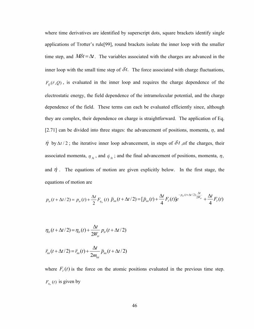
46

where time derivatives are identified by superscript dots, square brackets identify single

applications of Trotter’s rule[99], round brackets isolate the inner loop with the smaller

time step, and ttM Δ=δ . The variables associated with the charges are advanced in the

inner loop with the small time step of .tδ The force associated with charge fluctuations,

),( QrFQv , is evaluated in the inner loop and requires the charge dependence of the

electrostatic energy, the field dependence of the intramolecular potential, and the charge

dependence of the field. These terms can each be evaluated efficiently since, although

they are complex, their dependence on charge is straightforward. The application of Eq.

[2.71] can be divided into three stages: the advancement of positions, momenta, ,η and

η& by 2/tΔ ; the iterative inner loop advancement, in steps of tδ ,of the charges, their

associated momenta, fqη , and fqη& ; and the final advancement of positions, momenta, ,η

and η& . The equations of motion are given explicitly below. In the first stage, the

equations of motion are

)(2

)()2/( tFttpttptrtrtr η

Δ+=Δ+ )(

4)](

4)([)2/( 2

)2/(tFtetFttpttp r

Wtttp

riitr

tr

vvvv Δ

+Δ

+=Δ+Δ

Δ+−

αα

)2/(2

)()2/( ttpW

tttt trtr

trtr Δ+Δ

+=Δ+ ηη

)2/(2

)()2/( ttpm

ttrttr ii

ii Δ+Δ

+=Δ+ αα

ααvvv

where )(tFrv is the force on the atomic positions evaluated in the previous time step.

)(tFtrη is given by

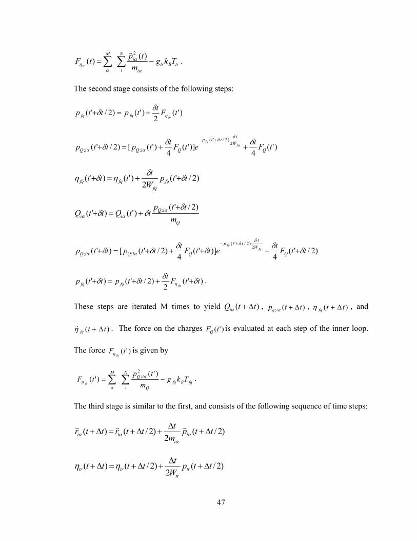
47

trBtr

N

i i

iM

Tkgm

tptFtr

−= ∑∑α

α

αη

)()(2v

.

The second stage consists of the following steps:

)'(2

)'()2/'( tFttpttpfqfqfq η

δδ +=+

)'(4

)]'(4

)'([)2/'( 2)2/'(

;; tFtetFttpttp QW

tttp

QiQiQfq

fq δδδδ

δ

αα ++=++−

)2/'(2

)'()'( ttpW

tttt fqfq

fqfq δδηδη ++=+

Q

iQii m

ttpttQttQ

)2/'()'()'( ; δ

δδ ααα

++=+

)2/'(4

)]'(4

)2/'([)'( 2)2/'(

;; ttFtettFtttpttp QW

tttp

QiQiQfq

fq

δδδδδδδ

δ

αα +++++=++−

)'(2

)2/'()'( ttFtttpttpfqfqfq δδδδ η +++=+ .

These steps are iterated M times to yield )( ttQi Δ+α , )(; ttp iq Δ+α , )( ttfq Δ+η , and

)( ttfq Δ+η& . The force on the charges )'(tFQ is evaluated at each step of the inner loop.

The force )'(tFfqη is given by

fqBfq

N

i Q

iQM

Tkgm

tptF

fq−= ∑∑

)'()'(

2; α

αη .

The third stage is similar to the first, and consists of the following sequence of time steps:

)2/(2

)2/()( ttpm

tttrttr ii

ii Δ+Δ

+Δ+=Δ+ αα

ααvvv

)2/(2

)2/()( ttpW

ttttt trtr

trtr Δ+Δ

+Δ+=Δ+ ηη

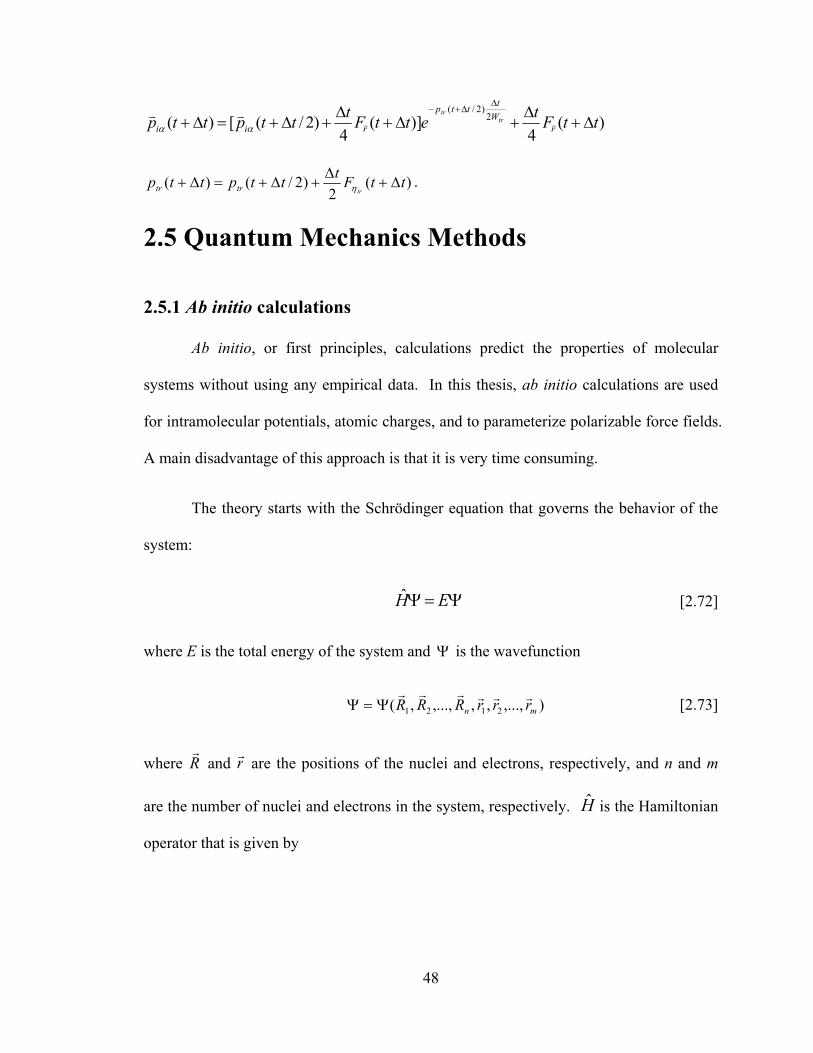
48

)(4

)](4

)2/([)( 2)2/(

ttFtettFtttpttp rW

tttp

riitr

tr

Δ+Δ

+Δ+Δ

+Δ+=Δ+Δ

Δ+−vv

vvαα

)(2

)2/()( ttFtttpttptrtrtr Δ+

Δ+Δ+=Δ+ η .

2.5 Quantum Mechanics Methods

2.5.1 Ab initio calculations

Ab initio, or first principles, calculations predict the properties of molecular

systems without using any empirical data. In this thesis, ab initio calculations are used

for intramolecular potentials, atomic charges, and to parameterize polarizable force fields.

A main disadvantage of this approach is that it is very time consuming.

The theory starts with the Schrödinger equation that governs the behavior of the

system:

Ψ=Ψ EH [2.72]

where E is the total energy of the system and Ψ is the wavefunction

),...,,,,...,,( 2121 mn rrrRRR rrrrrrΨ=Ψ [2.73]

where Rr

and rr are the positions of the nuclei and electrons, respectively, and n and m

are the number of nuclei and electrons in the system, respectively. H is the Hamiltonian

operator that is given by

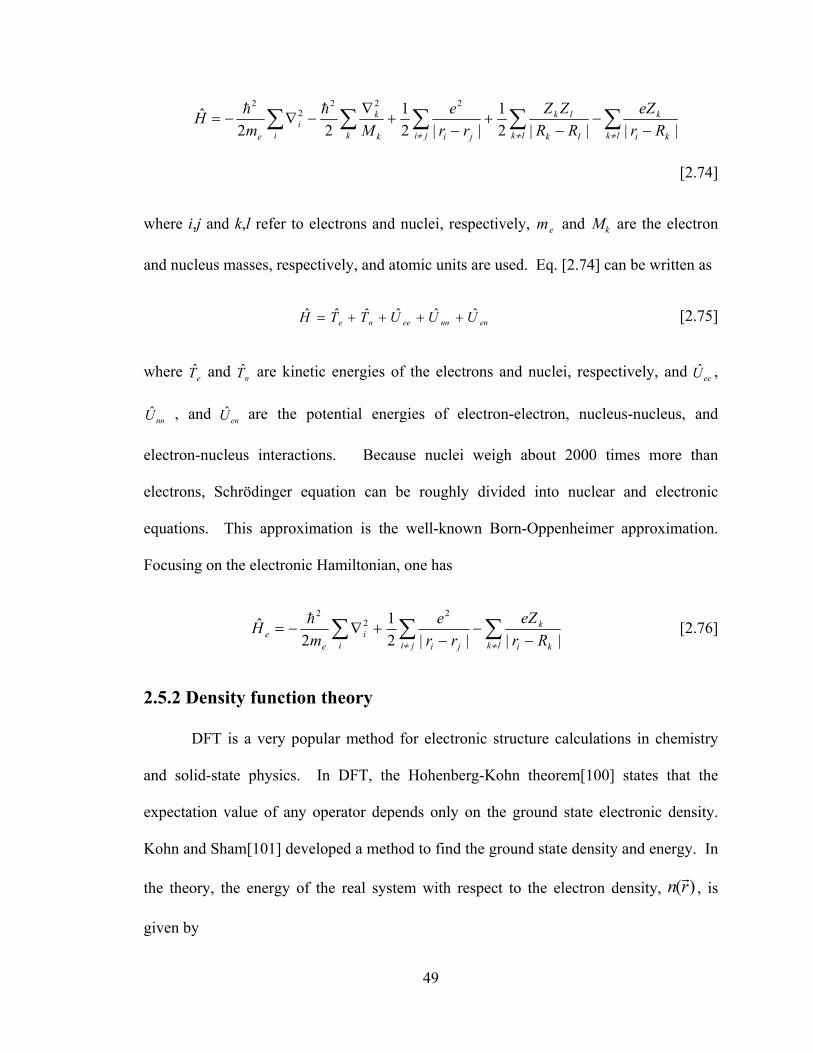
49

∑∑∑∑∑≠≠≠ −

−−

+−

+∇

−∇−=lk ki

k

lk lk

lk

ji jik k

k

ii

e RreZ

RRZZ

rre

MmH

||||21

||21

22ˆ

2222

2 hh

[2.74]

where i,j and k,l refer to electrons and nuclei, respectively, em and kM are the electron

and nucleus masses, respectively, and atomic units are used. Eq. [2.74] can be written as

ennneene UUUTTH ˆˆˆˆˆˆ ++++= [2.75]

where eT and nT are kinetic energies of the electrons and nuclei, respectively, and eeU ,

nnU , and enU are the potential energies of electron-electron, nucleus-nucleus, and

electron-nucleus interactions. Because nuclei weigh about 2000 times more than

electrons, Schrödinger equation can be roughly divided into nuclear and electronic

equations. This approximation is the well-known Born-Oppenheimer approximation.

Focusing on the electronic Hamiltonian, one has

∑∑∑≠≠ −

−−

+∇−=lk ki

k

ji jiii

ee Rr

eZrr

em

H||||2

12

ˆ2

22h [2.76]

2.5.2 Density function theory

DFT is a very popular method for electronic structure calculations in chemistry

and solid-state physics. In DFT, the Hohenberg-Kohn theorem[100] states that the

expectation value of any operator depends only on the ground state electronic density.

Kohn and Sham[101] developed a method to find the ground state density and energy. In

the theory, the energy of the real system with respect to the electron density, )(rn r, is

given by

50

][][][][ nUnVnTnE ++= [2.77]

where ][nT is the kinetic energy, ][nU is the two-body electron-electron interaction, and

∫= rdrnrVnV rrr 3)()(][ is the energy due to the external potential from the nuclei. To

minimize the energy functional, it can be written as a density functional of non-

interacting particles:

][||][][ nVTnnE sssss ψψ += [2.78]

where sT is the kinetic energy of the non-interacting electrons, sV is the external

potential, and the density of the non-interacting system, )(rnsr , is equal to the density of

interest, )(rn r. The full ground state energy of a real system is written as

∑∑ ∇−−==i

KSi

KSird

rrnZnEE )1(||)1(

21)(][ 2

111

1000 θθ

α αα

rr

][)()(21

02112

2010 nErdrdr

rnrnxc++ ∫∫

rrrr

[2.79]

The first three terms are the electron-nuclear interaction energy, the average ground state

kinetic energy of non-interacting electrons, and the electron-electron interaction energy,

respectively. The last term, ][ 0nExc , is the Kohn-Sham exchange-correlation energy.

The exchange-correlation potential is the derivative of the exchange-correlation energy

)()]([)(

0

0

rnrnErV xc

xc r

rr

δδ

= [2.80]

51

The spatial part of Kohn-Sham orbital, KSiθ , is determined by solving the Kohn-Sham

equations of the non-interacting system iteratively:

)()()](21[ 2 rrrV KS

iiKS

isirrr θεθ =+∇− [2.81]

where iε are Kohn-Sham orbital energies and the electron density is given by

∑=i

KSi rrn 2|)(|)( rr θ .

An important problem of this method is that the Kohn-Sham exchange-correlation

functional xcE is unknown. One of the most popular exchange-correlation functionals is

the B3LYP, which is a hybrid functional combining the local-spin-density approximation

exchange functional[102], the Lee-Yang-Par correlation functional[103], and the Becke's

exchange functional[98], which is combined with the exact energy from Hartree-Fock

theory.

DFT generally gives accurate results for most properties such as molecular

geometries, frequencies and dipole moment, and is much more efficient than perturbation

theory, coupled cluster methods and Configuration Interaction method.

2.5.3 Basis sets

In quantum calculations, the molecular orbitals are represented by linear

combinations of basis functions:

∑=i

iii c χφ [2.82]

52

where iχ are atom-centered basis functions and ic are the variational coefficients. There

are many choices of basis functions. Slater type orbitals (STOs) are a natural choice, but

they are computationally expensive and impractical for nonlinear polyatomic systems.

An alternative to STOs is the Gaussian-type functions (GTFs). A Cartesian Gaussian

centered on a nucleus is defined as 2

,,rkji

kji ezyNxg α−= , where N is the normalization

coefficient, α is a positive orbital exponent, i,j,k are nonnegative integers, and x, y, z are

Cartesian coordinates with the origin at the nucleus. However, a single GTF cannot

reproduce an STO very well, because it has no cusp at the nucleus and decays to zero too

quickly. Thus, the contracted Gaussian-type functions (CGTFs) are more commonly

used. CGTFs, often referenced to as primitives, are linear combinations of GTFs and can

better reproduce the STOs. For example, in the STO-3G basis set, each STO is

reproduced by three GTFs. The minimal basis set has one basis function for each

occupied atomic orbital. Multiple-zeta basis set has multiple CGTFs for each occupied

atomic orbital. For instance, cc-pVDZ represents two CGTFs for each atomic orbital. A

more popular type of basis set is the split valence basis set, which applies multiple-zeta

basis functions to valence orbitals and single-zeta basis functions to core orbitals.

In molecules, atomic orbitals (AOs) are distorted. In order to account for this

shape distortion, additional Gaussian functions with high angular momenta, called

polarization functions, are required. For instance, 6-311G(d,p) basis set has 6 primitive

Gaussians for each inner-shell AO, and each valence-shell AO is represented by 3 CGTFs,

one formed by three pieces composed of three Gaussian primitives, one Gaussian

primitive, and one Gaussian primitive. The “(d,p)” denote that a set of 6 d-type Gaussian

functions is added to nonhydrogen atoms and a set of 3 p-type Gaussian functions is

53

added to hydrogen atoms. For some molecules, such as anions and those with lone pairs,

the electron density is still very significant at large distances from the nuclei. To improve

the accuracy of treating such molecules, highly diffuse functions with a very small orbital

exponent can be added. For instance, the aug-cc-pVDZ basis set augments the cc-pVDZ

basis by additional slowly decaying s, p and d Gaussian functions.

2.5.4 Atomic charges

There are many different definitions and algorithms to assign atomic

charges [104-109]. Mulliken population analysis approach [104-106, 108] is one of the

most often used. In this approach, atomic charges are assigned on the basis of atomic

orbital populations.

Another approach of obtaining atomic partial charges is to fit the molecular

electrostatic potential (MEP). The MEP at position 1rr

is:

∑ ∫−=α α

αφ 212

2

11

)()( rdrrn

rZr r

rr [2.83]

where αZ and )( 2rn r are the charge on nucleus α and the charge density at position 2rr ,

respectively, and the first and second terms are the nuclear and electronic part,

respectively. The atomic partial charges are fitted to reproduce the MEP at a number of

points:

∑=α α

αφ1

1)(rQrfitting r [2.84]

and the charges are obtained by least square fit to minimized the following

54

∑=

−=N

ii

calculatedi

fitting rrf1

2)]()([ rr φφ [2.85]

where N is the total number of points used in the MEP.

In this thesis, the CHarges from Electrostatic Potentials using a Grid based

method (CHELPG) scheme[110], which is one of the most common schemes, is used to

obtain atomic charges. We choose this scheme because the charges calculated by

CHELPG depend on the environment and the actual potential, which is a feature we want

to integrate into our simulation.

2.5.5 Conformational Minimization

In order to obtain the most stable molecular structures, conformational

minimization is needed to get the local energy minima. The potential energy surface of a

molecule has 3N-6 degrees of freedom, where N is the number of atoms in the molecule.

Starting from the input geometry, the potential energy and its first derivatives are

calculated and then the 3N-6 degrees of freedom are changed to get a lower potential

energy. This procedure is iterated until a local minimum is found. Large molecules

normally have many local minima, and in order to locate the global minimum, it is

necessary to repeat the search procedure for different starting geometries.

In this thesis, DFT calculations are used to obtain equilibrium structures and

intramolecular potentials of solvents, such as ethanol, benzyl alcohol, and 2-propanol.

B3LYP/6-311++G(d,p), B3LYP/6-311G(d,p) and B3LYP/aug-cc-pVDZ calculations are

performed for ethanol, benzyl alcohol, and 2-propanol, respectively. For ethanol, the

intramolecular motion is divided into 8 stretches, 13 bends, and 2 torsions. For benzyl

55

alcohol, since the aromatic ring is very rigid, only 5 stretches, 9 bends, 2 torsions, and 1

improper torsion are chosen to represent the molecular flexibility. For 2-propanol, 19

bends and 3 torsions are employed to represent intramolecular motion.

Each stretching force constant is extracted from nine energy calculations, as the

bond is compressed and stretched away from the equilibrium value. Bending potentials

are obtained by least squares fits to nine energy calculations where the angle is varied

within sixteen degrees of the equilibrium value. For torsion potentials, the angle is varied

from 0 to 360o, in steps of 10 degrees. Each of the improper torsion potentials is obtained

from nine restricted geometry optimizations.

DFT calculations are also used to obtain the FC and fCINTRA parameters. The

details will be described in Chapter 3.

2.6 Chirality indexes

The aim of this thesis is to study the transfer of chirality from chiral solutes or

surfaces to achiral solvents. Therefore, it is very important to find a way to quantify the

chirality. As introduced in the previous chapter, chirality indexes have been a subject of

continuing interest over the past fifteen years. Most of the proposed measures are not

suited to this particular study since the chirality measure employed here should be

evaluated from individual solvent molecules. The measure should also be unchanged by

a simple translation or rotation of the solvent, should change signs upon reflection,

should average to zero for solvent in an achiral environment, and should be fast to

calculate since millions of calculations will be required in MD simulations. With these

considerations, we use a chirality index which was originally developed by Osipov et

56

al[66]. Our implementation includes a modification introduced by Solymosi et al.[111]

to partially correct for a strong dependence on the number of atoms N in the molecule.

The chiral index is defined as:

[2.86]

where the sum runs over all combinations of four atoms in the molecule. The superscript

of wSG0 shows the type of atomic weights, where 1, q and m correspond to unity, atomic

charges and atomic masses, respectively. From Eq. [2.86], wSG0 has a strong dependence

on molecular structure, as reflected by the presence of interatomic vectors. Dependence

on other properties can be included via the atomic weights, wi , that can be chosen to be

atomic charges, van der Waals radii, atomic masses, and so on. The powers n and m in

the denominator of Eq. [2.86] can be chosen to emphasize the contributions from atoms

well separated within the molecule (small values for m and n) or atoms that are close

together (large values for m and n).

A strictly shape-dependent index can be obtained by choosing all weights equal to

unity in Eq. [2.86]. The resulting index, 10SG , gives equal weighting to all the atoms and

reflects only the asymmetry of the atomic positions. In addition to this index, we explore

indexes mSG0 and q

SG0 , where the weights are atomic masses and atomic charges,

respectively. The former will de-emphasize the hydrogen atoms and, for the ethanol, 2-

propanol, and benzyl alcohol solvents, terms involving the oxygen and carbon atoms will

contribute most to mSG0 . The latter index, where the terms are weighted by the atomic

charges, will place greater emphasis on the alcohol group of the solvents where the

57

atomic charges are largest. For 10 SG , when the powers m and n in Eq. [2.86] are set to 1

and 2, respectively, the index becomes dimensionless.

Regardless of the choice of atomic weights, or m and n, in Eq. [2.86], the indexes

are zero for an achiral solvent structure. To see the response of wSG0 to reflection,

consider the term ))(]()[( 34232312143412 rrrrrrr vvvvvvv ⋅⋅⋅× in Eq. [2.86]. If the mirror operation is

performed, ])[( 143412 rrr vvv ⋅× will change sign but )( 2312 rr vv ⋅ and )( 3423 rr vv ⋅ will stay the same,

and the whole term will change sign. Thus, all indexes obtained from Eq. [2.86] will

change sign for the mirror-image molecule. Within the simulations, this symmetry

ensures that all indexes will average to zero for solvents in an achiral environment. In

addition, translational and rotational invariance follows from Eq. [2.86] since the indexes

are determined from dot products of interatomic vectors and these are unchanged by

translation and molecular reorientation. Thus, as required, the instantaneous index

reflects the shape of the molecule but not its position or orientation.

Despite these important advantages, there is one important concern with the use

of wSG0 . As discussed by Solymosi[111], the index depends on the number of atoms in

the molecule: They introduced the N! term in Eq. [2.86] to partially eliminate this

dependence. Nonetheless, a residual dependence remains and we cannot compare the

magnitude of the excess chirality >< wSG0 for the two different solvents. However, we

are most interested in the impact of various chiral solutes on a given solvent and, for this,

< wSG0 > can be compared.

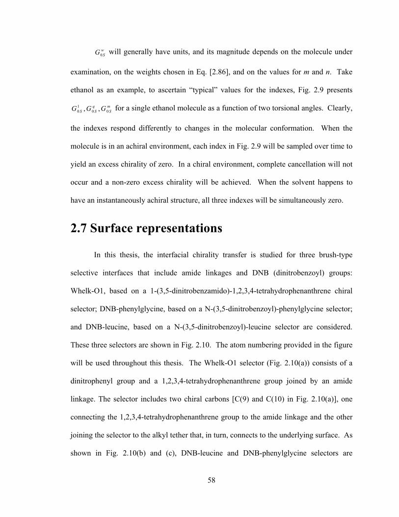
58

wSG0 will generally have units, and its magnitude depends on the molecule under

examination, on the weights chosen in Eq. [2.86], and on the values for m and n. Take

ethanol as an example, to ascertain “typical” values for the indexes, Fig. 2.9 presents

mS

qSS GGG 00

10 ,, for a single ethanol molecule as a function of two torsional angles. Clearly,

the indexes respond differently to changes in the molecular conformation. When the

molecule is in an achiral environment, each index in Fig. 2.9 will be sampled over time to

yield an excess chirality of zero. In a chiral environment, complete cancellation will not

occur and a non-zero excess chirality will be achieved. When the solvent happens to

have an instantaneously achiral structure, all three indexes will be simultaneously zero.

2.7 Surface representations

In this thesis, the interfacial chirality transfer is studied for three brush-type

selective interfaces that include amide linkages and DNB (dinitrobenzoyl) groups:

Whelk-O1, based on a 1-(3,5-dinitrobenzamido)-1,2,3,4-tetrahydrophenanthrene chiral

selector; DNB-phenylglycine, based on a N-(3,5-dinitrobenzoyl)-phenylglycine selector;

and DNB-leucine, based on a N-(3,5-dinitrobenzoyl)-leucine selector are considered.

These three selectors are shown in Fig. 2.10. The atom numbering provided in the figure

will be used throughout this thesis. The Whelk-O1 selector (Fig. 2.10(a)) consists of a

dinitrophenyl group and a 1,2,3,4-tetrahydrophenanthrene group joined by an amide

linkage. The selector includes two chiral carbons [C(9) and C(10) in Fig. 2.10(a)], one

connecting the 1,2,3,4-tetrahydrophenanthrene group to the amide linkage and the other

joining the selector to the alkyl tether that, in turn, connects to the underlying surface. As

shown in Fig. 2.10(b) and (c), DNB-leucine and DNB-phenylglycine selectors are

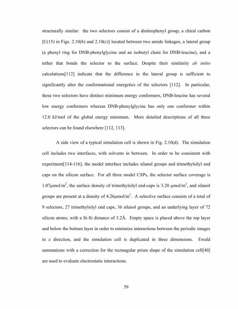
59

structurally similar: the two selectors consist of a dinitrophenyl group, a chiral carbon

[C(15) in Figs. 2.10(b) and 2.10(c)] located between two amide linkages, a lateral group

(a phenyl ring for DNB-phenylglycine and an isobutyl chain for DNB-leucine), and a

tether that bonds the selector to the surface. Despite their similarity ab initio

calculations[112] indicate that the difference in the lateral group is sufficient to

significantly alter the conformational energetics of the selectors [112]. In particular,

these two selectors have distinct minimum energy conformers, DNB-leucine has several

low energy conformers whereas DNB-phenylglycine has only one conformer within

12.0 kJ/mol of the global energy minimum. More detailed descriptions of all three

selectors can be found elsewhere [112, 113].

A side view of a typical simulation cell is shown in Fig. 2.10(d). The simulation

cell includes two interfaces, with solvents in between. In order to be consistent with

experiment[114-116], the model interface includes silanol groups and trimethylsilyl end

caps on the silicon surface. For all three model CSPs, the selector surface coverage is

1.07µmol/m2, the surface density of trimethylsilyl end-caps is 3.20 µmol/m2, and silanol

groups are present at a density of 4.26µmol/m2. A selective surface consists of a total of

9 selectors, 27 trimethylsilyl end caps, 36 silanol groups, and an underlying layer of 72

silicon atoms, with a Si-Si distance of 3.2Å. Empty space is placed above the top layer

and below the bottom layer in order to minimize interactions between the periodic images

in z direction, and the simulation cell is duplicated in three dimensions. Ewald

summations with a correction for the rectangular prism shape of the simulation cell[40]

are used to evaluate electrostatic interactions.

60

Figure 2.9. The influence of torsional angles on chirality indexes of ethanol. Panel (a) shows the two torsions under consideration. For the conformation shown in Panel (a), both torsion 1 and torsion 2 are 180 degrees. Panels (b), (c), and (d) show 1

OSG , qOSG , m

OSG , respectively, as the torsional angles vary. The atomic charges from the ab initio calculations are used for (b). Panel (e) presents q

OSG for a different set of average atomic charges observed in the simulations.

61

Figure 2.10. Molecular structures and numbering system for (a) Whelk-O1, (b) DNB-leucine, (c) DNB-phenylglycine. The atom numbering will be used throughout this chapter. Panel (d) provides a side view of a typical simulation cell. In this case, the Whelk-O1 surface in the presence of ethanol is shown. Silicon, oxygen, hydrogen, nitrogen, and carbon are shown in yellow, red, white, blue, and grey respectively. Solvent atoms are shown in wireframe. Please note that the hydrogen atoms connected to achiral carbons are omitted for simplicity.

62

Within the simulations, the chiral selectors are semi-flexible. In particular, the

rings are kept rigid while the rest of the molecule is flexible. The atoms within these

rigid units do not move relative to each other but rather they collectively translate and

rotate according to their aggregate forces. The conserved quantity in the simulations is

the Nosé-Hoover Hamiltonian (HNH), which is defined in Eq. [2.58].

2.8 Practical considerations

All the simulations were performed using the MDMC program that originated from

our group. Prior to this work, the MDMC program had been applied to simulations of bulk

phases and interfacial systems using non-polarizable models. To achieve the objectives of

this thesis, the program has been modified extensively to include the charge fluctuation

model, the field-dependent intramolecular potential, the multiple time step algorithm, and

chirality index collection.

The charge fluctuation model requires additional force calculations and new

equations of motion, so the relevant part of the program has been modified. The field-

dependent intramolecular potential requires new force calculation subroutines and a

multiple time scale approach. For the latter, each inner step requires force calculations,

which is very time-consuming. Therefore, much effort has been used to improve the

efficiency of the calculations.

The non-bonding force calculations and the evaluation of forces from the field-

dependent intramolecular potential are the most time-consuming aspects of the

63

computation. We have parallelized this segment of the code to allow for rapid

computation of the forces. More specifically, the message-passing interface (MPI) has

been employed. The message passing model is defined as a set of processes that have

local memory and communicate with each other by sending and receiving messages. In

the simulation program, a master/slave model is used. All the serial work, such as the

initialization and input/output, is done on the master node. Also, the computationally

inexpensive parts of the simulation, such as the intramolecular force calculation and

integration of equations of motion, are done on the master node. The time-consuming

parts of the simulation, such as the LJ forces and Ewald summation, are implemented in

parallel on both master and slave nodes. In each time step, the master node distributes

the task evenly on all processes and sends the necessary information to all the slave nodes

using broadcast statements. After calculations are done, all nodes send their part back to

the master node, which then sums up the results. The implementation of MPI in the

simulation has been optimized to minimize the communication time. Our simulations are

performed on High Performance Computing Virtual Laboratory (HPCVL), Westgrid and

SHARCNET high performance computing facilities. Most of the single processor

simulations are performed on Westgrid (Glacier) and most of the MPI simulations are

performed on Requin and Narwhal clusters of SHARCNET. Our parallel simulations use

8 processors and are about 7.5 times as fast as simulations with single processor. About

20-30 independent simulations are performed for each solute/solvent and surface/solvent

pair and, as a rough guide, each simulation requires roughly two weeks of simulation

time.

64

Chapter 3 Development of a polarizable and flexible model

Intuitively, chirality transfer and polarization are closely related. In this chapter,

methodology for developing a polarizable and flexible model (the fCINTRA model) is

discussed in detail. All aspects of the model design are discussed along with details of

the simulations, including the implementation of a multiple time step molecular dynamics

algorithm. This methodology is general and can be applied to any molecules. In this

chapter, an example has been provided for ethanol and the results of MD simulations

with this model are analyzed and compared with experiments and other popular models.

3.1 Introduction

Hydrogen bonding in alcohols is complex and quite different from bulk

water [117]. Neutron diffraction[118], ab initio calculations[119], and simulations[120]

show that bulk methanol under supercritical conditions is characterized by monomers and

small hydrogen-bonded rings. Under ambient conditions, it has been suggested[121] that

methanol prefers closed-chain hydrogen-bonded hexamers. The situation is less clear for

ethanol[117, 122] where hydrogen-bonded networks have been assumed to prefer

tetrameric loops, hexameric loops, U-shapes, or coils. A recent neutron diffraction[123]

study, along with previous X-ray[124] and neutron diffraction[125] work on ethanol,

provides increasingly accurate experimental interatomic distributions in the bulk.

Ethanol has also been the subject of several statistical mechanics studies [43, 45, 126,

65

127]. The simplest molecular models for ethanol[128, 129] have fixed-charges on the

atoms and are pairwise-additive. Fixed-charge transferable potentials, such as

OPLS[127], have been well studied for alcohols[127]. The use of fixed charges means

that the molecules are not polarized by the local electric field: An important effect for

hydrogen-bonded liquids[47].

The importance of polarizability, and the impact of its inclusion, are well

understood for water where a variety of polarizable models have been designed [42, 46,

47, 130]. In this thesis, we employ the FC model to govern the atomic charge

fluctuations in bulk ethanol. Relative to other polarizable models, ours is unique in one

important respect: It includes field dependence in both the atomic charges and the

intramolecular degrees of freedom. In this way, the model reflects the field-induced

redistribution of electrons that results in instantaneous changes to atomic charges and to

the potential energy surface that defines intramolecular motion. This is particularly

important for the torsional motion governing the position of the hydrogen-bonding

hydrogen: We find that this potential is highly field-dependent and, in some fields the

minima appear at very different angles relative to the zero-field potential. Thus, the

optimal position of the hydrogen depends on the field experienced by the molecule and

this will, in turn, influence the hydrogen bonding structure in the fluid. As mentioned in

Chapter 1, a field-dependent intramolecular potential has been attempted only once

previously. In that study, the HH and OH stretching potentials of water depended on the

magnitude of the field of oxygen but the atomic charges were field-independent [57].

Aside from this one exception, existing polarizable flexible models fully separate the

molecular flexibility from the field response.

66

Persuasive arguments for a systematic application of the FC method have been

presented by Patel and Brooks[53] and Banks et al.[131] Our implementation of the FC

method differs primarily in that we rely exclusively on ab initio results to describe the

atomic charge fluctuations. The field-dependent intramolecular potentials are also

derived strictly from ab initio results. Overall, we have placed considerable emphasis on

developing a methodology that can be readily extended to other molecules. In particular,

relatively few parameters remain to be determined empirically and these are optimized by

comparison with experimental interatomic distributions for bulk ethanol[123] and by

comparison with the measured self-diffusion coefficient[87], dielectric constant[132], and

enthalpy of vaporization[133]. The simultaneous implementation of field-dependent

atomic charges and intramolecular potentials impacts the equations of motion for the

fluid and the simulations are significantly more lengthy than for corresponding non-

polarizable models.

Results from extensive molecular dynamics simulations of bulk ethanol are

reported. In particular, the hydrogen bonding network is examined in detail. We

compare our results with a non-polarizable ethanol model, a partially polarizable model

where the intramolecular motion is field-independent but atomic charges respond to the

electric field, and a partially polarizable model where the atomic charges are field-

independent but the intramolecular potential responds to the electric field.

This chapter is organized as follows. Section 3.2 outlines the methods we have

used to arrive at the polarizable flexible model for ethanol. Section 3.3 analyzes the fluid

structure and properties, with an emphasis on hydrogen bonding. Concluding remarks

are given in Section 3.4.

67

3.2. Methods

The full field-dependent potential, )(EUr

, is written as

LJel UEUEUEU ++= )()()( intrarrr

[3.1]

where the evaluation of the electrostatic energy, )(EU elr

, is discussed in Section 3.2.3.

The field-dependent intramolecular potential, )(intra EUr

, is the subject of Section 3.2.5.

The Lennard-Jones contribution to the energy, LJU , is not field-dependent and has been

discussed in Chapter 2.

Fig. 2.8 shows the atom labeling employed throughout this chapter. The model

developed in this chapter is referred to as the Fluctuating Charge and INTRAmolecular

potential (fCINTRA) model. A flowchart summarizing our procedure for ethanol model

development is given in Fig. 3.1.

The process begins by assessing the range and frequency of fields experienced in

bulk ethanol. As shown in Fig. 3.1, molecular dynamics simulations using a non-

polarizable model are used to provide an estimate of “typical” fields in bulk ethanol. The

second and third steps in our procedure involve the analysis of the collected fields and the

selection of a representative subset. Steps 1-3 in Fig. 3.1 are discussed in detail in

Section 3.2.1 below. The field-response of ethanol molecules is assessed via an extensive

series of ab initio calculations. A very large number of calculations is required and, as a

result, the ab initio method chosen to evaluate field response must be efficient as well as

accurate. Thus, benchmarking against high level calculations is a necessary step to

choose the appropriate basis set and method used to quantify the molecular response.

The discussion of the ab initio calculations is provided in Section 3.2.2. Following these

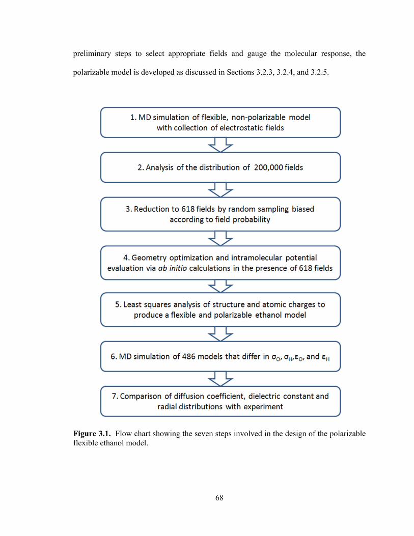
68

preliminary steps to select appropriate fields and gauge the molecular response, the

polarizable model is developed as discussed in Sections 3.2.3, 3.2.4, and 3.2.5.

Figure 3.1. Flow chart showing the seven steps involved in the design of the polarizable flexible ethanol model.

69

3.2.1 Assessment of typical electric fields in bulk ethanol

In the parameterization of a polarizable model, a limited number of fields can be

explicitly considered. We chose to proceed by directly assessing the fields a typical

ethanol molecule experiences in the bulk. Specifically, a lengthy molecular dynamics

simulation of bulk ethanol was undertaken. The flexible non-polarizable model of Chen

et al.[134] was employed with fields recorded every 500 time steps. The simulations

were performed in the NVE ensemble, for 2000 molecules, over 50000 iterations, and

with a time step of 0.127 fs. Ewald[90] sums were employed, with tinfoil boundary

conditions, a convergence parameter α of 0.1609 Å-1, and a momentum space cutoff of

k*2 ≤ 27.

Throughout the simulation, the field on the C(3), O(2), and H(1) atoms of each

molecule were monitored. Information was not gathered for the other atoms since C(4) is

uncharged in the Chen et al.[134] model and the other hydrogens do not appear explicitly

in the model. The end result, summarized in Fig. 3.2, is a distribution of electric fields in

bulk ethanol, as predicted from a non-polarizable ethanol model. While the field

distributions will change for a polarizable model, Fig. 3.2 provides a rough estimate of

the range of fields experienced by ethanol molecules in the bulk, and the probability of a

given field. It is important to note that long-ranged contributions to these fields are

substantial. Thus, the intuitive process of generating fields by placing charges at

hydrogen-bonding sites[131], or other local sites, will not produce typical fields

experienced by ethanol molecules in the bulk liquid.

The 200,000 fields summarized in Fig. 3.2 are too numerous to consider directly.

The number of fields is reduced to 618 as follows. Figs. 3.2(a), 3.2(b), and 3.2(c) are

70

individually employed to select 350, 158, and 110 fields, respectively, from the 200000

possibilities. Consider Fig. 3.2(a). We divide the magnitude of the field squared, E2, on

C(3) into 2000 equal segments. For a given E2 range, 405 to 405.5 say, the height of the

curve is compared to the maximum. If a random number is less than this ratio then one

of the fields with an E2 in this range will be selected for further analysis. In this way, the

field selection is biased by the frequency of occurrence of the field. The procedure is

repeated for Figs. 3.2(b) and 3.2(c). Note that the broader peak in Fig. 3.2(a) results in a

larger number of selected fields. Distributions corresponding to the 618 fields are shown

in Fig. 3.2. The desired result has been achieved: a manageable number of fields,

representative of typical fields experienced by ethanol molecules in the bulk.

3.2.2 Ab initio calculations for molecular response

The parameterization of molecular response to a given field requires that the field

be reproduced in the ab initio calculation. Here, the field is obtained by placing four

point charges around a single ethanol molecule with the magnitudes and positions of the

charges chosen to reproduce the fields at C(3), O(2), and H(1). In practice, the charges

must be far enough from the molecule so that the molecule responds to an overall field

rather than to individual charges. We accomplish this by excluding the charges from the

volume defined by a box of dimensions 2(xmax,ymax,zmax), where xmax, ymax, and zmax are

the largest components of the atomic positions. This procedure is repeated for 618 fields

and a set of four point charges is obtained for each field.

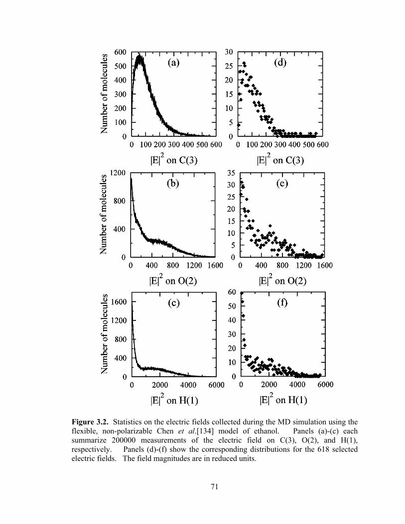
71

Figure 3.2. Statistics on the electric fields collected during the MD simulation using the flexible, non-polarizable Chen et al.[134] model of ethanol. Panels (a)-(c) each summarize 200000 measurements of the electric field on C(3), O(2), and H(1), respectively. Panels (d)-(f) show the corresponding distributions for the 618 selected electric fields. The field magnitudes are in reduced units.

72

In a bulk liquid, the molecule cannot rotate or translate fast enough to respond to

an instantaneous change in the field, but its atomic charges and potential surface change.

That is, the electrons rapidly move about the molecule to respond to the field but the

nuclei respond much more slowly. A full optimization of the molecular structure in the

presence of a field would lead to translation and rotation. In order to prevent this, C(3) is

forced to remain at the origin, O(2) must lie on the z-axis, and H(1) is in the xz plane

during the optimization. These constraints prohibit translation and, to a large extent,

rotation due to the field. Other than these constraints, the molecule is fully optimized.

All ab initio calculations are performed using Gaussian 03[135]. Before selecting

a basis set and method, benchmark calculations were performed. Specifically, 16 fields

were selected randomly and the molecular structure was optimized in each of these fields,

for 20 functional/basis set combinations. In addition, for each field, a benchmark

calculation was performed using 2nd order Moller-Plesset perturbation theory[136] (MP2)

with the augmented correlation consistent triple-zeta (aug-cc-pVTZ) basis set of Dunning

et al.[137, 138] Table 3.1 shows the average error in the molecular dipole, relative to the

benchmark, for the 20 functional/basis set combinations. Specifically, for each

combination, the ratio

20,2,2

2,2,16

1 )()(

161

MPFMP

FMPFMethod

F μμμμ

−−∑

=

[3.2]

is calculated. FMethod ,μ and FMP ,2μ are the dipole moments obtained in the field for the

selected functional/basis set combination and for the benchmark, respectively, and 0,2MPμ

is the zero-field dipole. Table 3.1 clearly shows the importance of basis set on the

response: All of the basis sets are large, but additional polarization and diffuse functions

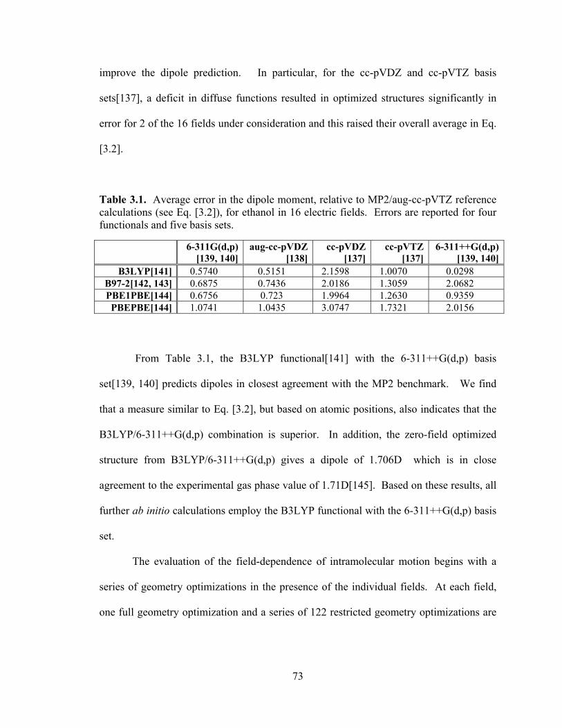
73

improve the dipole prediction. In particular, for the cc-pVDZ and cc-pVTZ basis

sets[137], a deficit in diffuse functions resulted in optimized structures significantly in

error for 2 of the 16 fields under consideration and this raised their overall average in Eq.

[3.2].

Table 3.1. Average error in the dipole moment, relative to MP2/aug-cc-pVTZ reference calculations (see Eq. [3.2]), for ethanol in 16 electric fields. Errors are reported for four functionals and five basis sets.

6-311G(d,p)[139, 140]

aug-cc-pVDZ[138]

cc-pVDZ[137]

cc-pVTZ [137]

6-311++G(d,p)[139, 140]

B3LYP[141] 0.5740 0.5151 2.1598 1.0070 0.0298B97-2[142, 143] 0.6875 0.7436 2.0186 1.3059 2.0682PBE1PBE[144] 0.6756 0.723 1.9964 1.2630 0.9359PBEPBE[144] 1.0741 1.0435 3.0747 1.7321 2.0156

From Table 3.1, the B3LYP functional[141] with the 6-311++G(d,p) basis

set[139, 140] predicts dipoles in closest agreement with the MP2 benchmark. We find

that a measure similar to Eq. [3.2], but based on atomic positions, also indicates that the

B3LYP/6-311++G(d,p) combination is superior. In addition, the zero-field optimized

structure from B3LYP/6-311++G(d,p) gives a dipole of 1.706D which is in close

agreement to the experimental gas phase value of 1.71D[145]. Based on these results, all

further ab initio calculations employ the B3LYP functional with the 6-311++G(d,p) basis

set.

The evaluation of the field-dependence of intramolecular motion begins with a

series of geometry optimizations in the presence of the individual fields. At each field,

one full geometry optimization and a series of 122 restricted geometry optimizations are

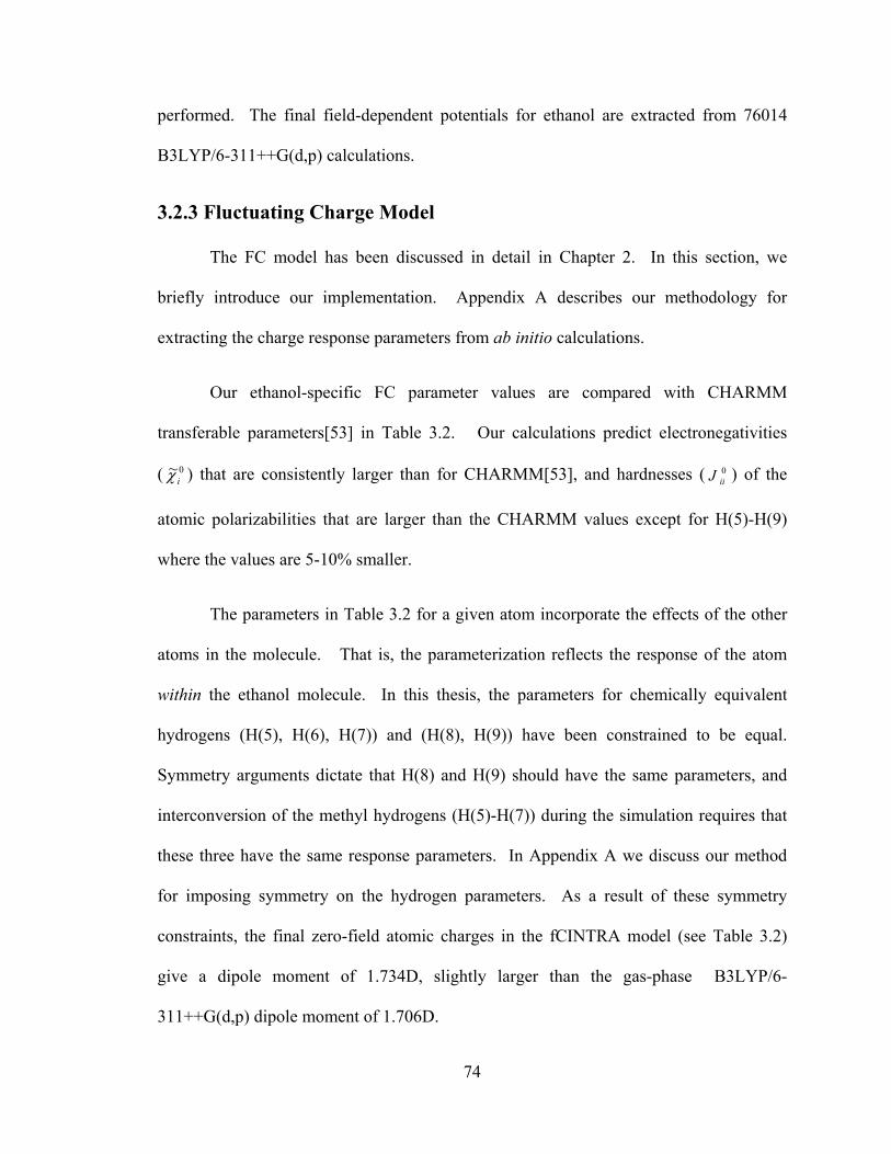
74

performed. The final field-dependent potentials for ethanol are extracted from 76014

B3LYP/6-311++G(d,p) calculations.

3.2.3 Fluctuating Charge Model

The FC model has been discussed in detail in Chapter 2. In this section, we

briefly introduce our implementation. Appendix A describes our methodology for

extracting the charge response parameters from ab initio calculations.

Our ethanol-specific FC parameter values are compared with CHARMM

transferable parameters[53] in Table 3.2. Our calculations predict electronegativities

( 0~iχ ) that are consistently larger than for CHARMM[53], and hardnesses ( 0

iiJ ) of the

atomic polarizabilities that are larger than the CHARMM values except for H(5)-H(9)

where the values are 5-10% smaller.

The parameters in Table 3.2 for a given atom incorporate the effects of the other

atoms in the molecule. That is, the parameterization reflects the response of the atom

within the ethanol molecule. In this thesis, the parameters for chemically equivalent

hydrogens (H(5), H(6), H(7)) and (H(8), H(9)) have been constrained to be equal.

Symmetry arguments dictate that H(8) and H(9) should have the same parameters, and

interconversion of the methyl hydrogens (H(5)-H(7)) during the simulation requires that

these three have the same response parameters. In Appendix A we discuss our method

for imposing symmetry on the hydrogen parameters. As a result of these symmetry

constraints, the final zero-field atomic charges in the fCINTRA model (see Table 3.2)

give a dipole moment of 1.734D, slightly larger than the gas-phase B3LYP/6-

311++G(d,p) dipole moment of 1.706D.

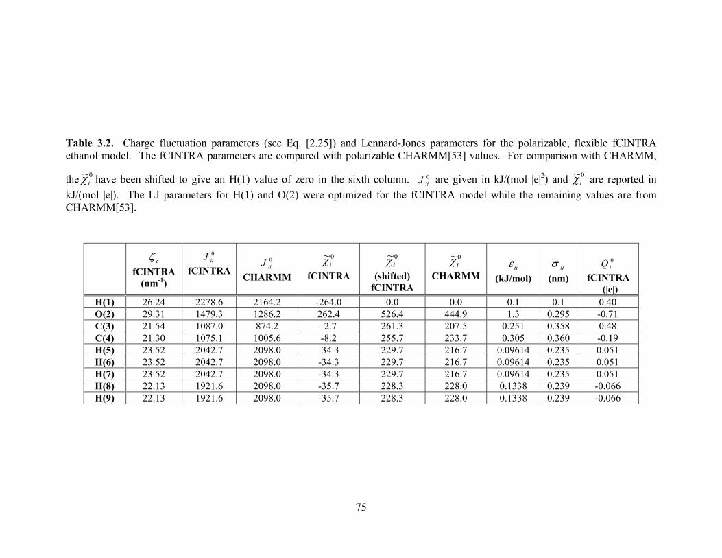
75

Table 3.2. Charge fluctuation parameters (see Eq. [2.25]) and Lennard-Jones parameters for the polarizable, flexible fCINTRA ethanol model. The fCINTRA parameters are compared with polarizable CHARMM[53] values. For comparison with CHARMM,

the 0~iχ have been shifted to give an H(1) value of zero in the sixth column. 0

iiJ are given in kJ/(mol |e|2) and 0~iχ are reported in

kJ/(mol |e|). The LJ parameters for H(1) and O(2) were optimized for the fCINTRA model while the remaining values are from CHARMM[53].

iζ

fCINTRA (nm-1)

0iiJ

fCINTRA

0iiJ

CHARMM

0~iχ

fCINTRA

0~iχ

(shifted) fCINTRA

0~iχ

CHARMM

iiε

(kJ/mol)

iiσ

(nm)

0iQ

fCINTRA (|e|)

H(1) 26.24 2278.6 2164.2 -264.0 0.0 0.0 0.1 0.1 0.40O(2) 29.31 1479.3 1286.2 262.4 526.4 444.9 1.3 0.295 -0.71C(3) 21.54 1087.0 874.2 -2.7 261.3 207.5 0.251 0.358 0.48C(4) 21.30 1075.1 1005.6 -8.2 255.7 233.7 0.305 0.360 -0.19H(5) 23.52 2042.7 2098.0 -34.3 229.7 216.7 0.09614 0.235 0.051H(6) 23.52 2042.7 2098.0 -34.3 229.7 216.7 0.09614 0.235 0.051H(7) 23.52 2042.7 2098.0 -34.3 229.7 216.7 0.09614 0.235 0.051H(8) 22.13 1921.6 2098.0 -35.7 228.3 228.0 0.1338 0.239 -0.066H(9) 22.13 1921.6 2098.0 -35.7 228.3 228.0 0.1338 0.239 -0.066

76

As described in Chapter 2, )( βαjiij rJ can be defined as a Coulomb overlap integral

(Eq. [2.27]) or using an approximation form (Eq. [2.29]). In Fig. 3.3, we compare the

H(1)-H(1) radial distribution from two simulations that differ only in the form of )( ijij rJ

for intramolecular atomic pairs separated by less than four bonds. From the figure, even

small changes in the )( ijij rJ lead to important differences in the fluid structure. In

particular, the fluid is less structured when Eq. [2.29] is employed and the average dipole

is 1.9 D. The experimental dipole moment in the bulk is 3.04 D[145] and the use of

)( ijij rJ from Eq. [2.27] gives an average dipole of 2.64 D. It appears that seemingly

small differences in the Coulomb overlaps can lead to significant differences in the fluid

structure and properties.

Figure 3.3. The impact of the representation of the interatomic Coulomb interaction, )( ijij rJ . The H(1)-H(1) radial distribution is shown for bulk ethanol at ρ=0.787 g/cm3

and T=298K. Results for the fCINTRA model with the overlap integral (Eq. [2.27]) form of the Coulomb interaction are given by a solid line, while use of Eq. [2.29] leads to the distribution identified by the dotted line.

77

3.2.4 Lennard-Jones potentials

The Lennard-Jones energy and length parameters, ijε and ijσ , are the only

adjustable parameters in our simulations: All other parameters are extracted from

B3LYP/6-311++G(d,p) calculations. In fact, we adjust only the LJ parameters for O(2)

and H(1), all others are taken from the CHARMM force field[53].

3.2.5 Intramolecular potentials

The functional forms for the stretch, bend, and torsion potentials have been

introduced in Chapter 2. For ethanol, we divide the intramolecular motion into 8

stretches, 13 bends, and 2 torsions, and the corresponding potentials are described by Eqs.

[2.31]-[2.33]. For Eq. [2.33], a form with a slight variation is used

, [3.3]

The ab initio energies used to define the potentials should be corrected[146], prior

to further analysis, by removing contributions from atoms separated by more than 3

bonds. For ethanol, this contribution is only from H(1) interacting with H(5)-H(7). Bond

lengths and angles do not change much during a simulation and the corrections will be

slowly varying over the relevant parameter range. Consequently, we have not corrected

the ab initio potentials for stretches and bends. Consider the torsions. The largest

contribution to the correction is expected from electrostatic interactions between the

hydrogens. We correct the ab initio energies as follows. For each torsional angle and

field, we subtract the electrostatic contribution to the energy, elU , as given in Eq. [2.26].

78

The atomic charges required for this correction are obtained by solving the equations of

motion for the charges (see Section 3.2.6 and Appendix B) for a single molecule

constrained to the appropriate geometry and in the chosen field. In this way, the

electrostatic contribution to the energy from atoms separated by more than three bonds,

as it is evaluated during a simulation, is removed from the ab initio energy.

The incorporation of field dependence in the coefficients of Eqs. [2.31]-[2.33] is

challenging. As a first step, we fitted power series in the fields at each atom, the field

components at each atom, and products between field components. While the resulting

fits were of acceptable quality, most of the individual terms were not physically

meaningful and the fitted potentials did not reproduce expected symmetry in the

potentials. Rather than pursue this approach, we have chosen to expand the field-

dependent parameters in Eqs. [2.31]-[2.33], according to “structural” analogs. These

terms are listed in Eqs. [2.35]-[2.43]. With these considerations in mind, the parameters

in Eqs. [2.31]-[2.33] are expanded using the terms in Eqs. [2.35]-[2.43] and the

multiplicative coefficients are obtained by least-squares fits with the SPSS package

(Version 13.0). The coefficients are prioritized and only the most significant are kept, so

that expansions for the individual coefficients are relatively short (11 terms or less). For

example, the equilibrium bond angle of H(1)-O(2)-C(3) is expanded as follows

...||1008.1|)||||(|1043.17.108)( 1231716154 +×−++×−= −−HOHHHHHHe EEEEE

rθ

[3.4]

Table 3.3 gives the expansion coefficients describing the field dependence of the

bond lengths. As described in Eqs. [2.41]-[2.42], X is used to represent atoms 8 and 9,

and Y denotes H(5), H(6), and H(7). Only the first term contributes in the absence of the

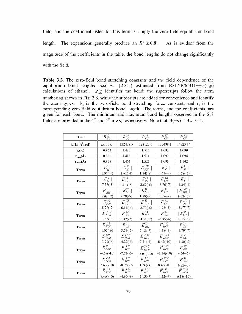
79

field, and the coefficient listed for this term is simply the zero-field equilibrium bond

length. The expansions generally produce an 8.02 ≥R . As is evident from the

magnitude of the coefficients in the table, the bond lengths do not change significantly

with the field.

Table 3.3. The zero-field bond stretching constants and the field dependence of the equilibrium bond lengths (see Eq. [2.31]) extracted from B3LYP/6-311++G(d,p) calculations of ethanol. AB

HOB identifies the bond: the superscripts follow the atom numbering shown in Fig. 2.8, while the subscripts are added for convenience and identify the atom types. ks is the zero-field bond stretching force constant, and re is the corresponding zero-field equilibrium bond length. The terms, and the coefficients, are given for each bond. The minimum and maximum bond lengths observed in the 618 fields are provided in the 4th and 5th rows, respectively. Note that nAnA −×=− 10)( .

Bond 12

HOB 23OCB 34

CCB YCHB 4 X

CHB 3

ks(kJ/Å2mol) 251105.1 132438.5 128123.6 157499.1 148234.4

re(Å) 0.962 1.430 1.517 1.093 1.099 rmin(Å) 0.961 1.416 1.514 1.092 1.094 rmax(Å) 0.978 1.464 1.526 1.098 1.102

Term || 1HE

1.07(-4) || X

HE 1.61(-4)

|| XXHHE

1.84(-6) || 3

CE 2.61(-5)

|| 1HE

1.68(-5)

Term || 2OE

-7.37(-5) || 11

HHE 1.04 (-5)

|| 24OCE

-2.60(-6)

XOHE 2

-8.76(-7) || 3

CE -1.24(-4)

Term || 11HHE

6.93(-7) || 22

OOE 2.78(-5)

|| 14HCE

1.98(-6)

31CHE

7.77(-7) || XX

HHE 9.22(-7)

Term 432CCOE

-8.79(-7) || XX

HHE -6.11(-6)

|| 89HHE

-2.77(-6)

XCHE 3

1.98(-6) || 2 X

OHE -6.37(-7)

Term 32X

HCOE -1.52(-6)

|| YXHHE

6.82(-7)

YOHE 2

-4.34(-7)

89HHE

-2.35(-6) || 32

COE 4.32(-6)

Term 34X

HCCE 1.02(-6)

21OHE

-3.53(-5)

YHHE 1

7.13(-7)

YYHCHE 4

1.18(-6) || 3Y

CHE -1.79(-7)

Term 839HCHE

-3.70(-6)

YYHCHE 4

-4.27(-6)

43YHCCE

2.51(-6)

32XHCOE

8.42(-10)

24OCE

-1.80(-5)

Term 321COHE)

-4.69(-10)

32XHCOE

-7.71(-6)

YYHCHE 4ˆ

-6.01(-10)

YYHCHE 4)

-2.14(-10)

YOHE 2

4.64(-6)

Term 432CCOE)

5.63(-10)

32XHCOE)

-8.98(-9)

32XHCOE)

1.26(-9)

32XHCOE)

8.42(-10)

89HHE

6.22(-7)

Term 34X

HCCE)

9.46(-10)

34XHCCE)

-4.93(-9)

34XHCCE)

2.13(-9)

839HCHE)

1.12(-9)

32XHCOE)

6.18(-10)

80

Table 3.4 gives the expansion coefficients for the field-dependence of the

equilibrium angles. The first coefficient in Table 3.4 is constrained to be the equilibrium

angle in the absence of a field. The other coefficients are obtained by regression. In

general, the fitted potentials provide a good representation of the bend potentials with the

exception of the H(1)-O(2)-C(3) angle. Even with a substantial number of expansion

terms the R2 is roughly 0.4. However, as indicated by the θmin and θmax values, this

angle does not vary much in the course of the simulation.

Consider the torsion about the O(2)-C(3) bond. This motion reflects the ease

with which the hydrogen-bonding hydrogen can rotate and will clearly be relevant to the

hydrogen bonding characteristics in the fluid. Fig. 3.4 shows this torsional potential in

six different fields. The uncorrected ab initio potential, the corrected potential obtained

by subtraction of the intramolecular electrostatic contribution, and the fitted potential are

compared. From the figure, the corrected and ab initio potentials are qualitatively similar.

However, the corrected potential has a higher barrier for rotation through the eclipsed

conformation in most fields. It is clear from the figure that some fields radically change

the characteristics of the torsion potential. For instance, in Fig. 3.4(d), in the presence of

this particular field, the minimum at 1800 has nearly disappeared. On the other hand,

many fields leave the potential virtually unchanged, as illustrated in Fig. 3.4(b). The

fitted potentials shown in the figure illustrate the overall quality of the fitted potentials:

very good agreement with the corrected ab initio potentials is shown in Figs. 3.4(a)-(c)

and poorer agreement is evident in Figs. 3.4(d) and 3.4(f). It is important to realize that

the curves are not fitted individually, rather a single functional form of the torsional

potential, Eq. [2.33], is used to model the response to all fields. That is, for 618 fields

81

and 35 energies on each potential curve a total of 21630 energies have been evaluated

and these are fitted simultaneously. As illustrated in Figs. 3.4(e) and 3.4(f), even for the

poorest fits, the fitted and corrected ab initio potentials are qualitatively similar. The

overall R2 value is 0.90. If we rank each field according to the quality of the fitted

torsional potential, then 390 fields have R2 values above 0.8. Only 94 fields have R2

values below 0.6. The expansion coefficients for the O(2)-C(3) torsion are given in

Table 3.5.

The field dependence of the torsion potential for rotation about the CC bond is

shown in Fig. 3.5. The methyl hydrogens are interchanged by this torsion and,

regardless of the applied field, interconversion of the hydrogens by a 120 degree rotation

forces the potential to return to its original value. The fields selected for the figure

illustrate the range of variability found for this potential. Clearly, the field has little

impact on this motion. As a result, we employ only the zero-field coefficients and these

have the following values (in kJ/mol): 183.70;2 =C , 798.211;2 −=C , 625.303;2 =C , and

644.15;2 −=C . All other coefficients in Eq. [2.33] are zero for this torsion and this field-

independent potential yields and R2 value of 0.975.

Within our simulations, we have focused on the more strongly field-dependent

motions. As a result, we have not considered the field dependence of the stretching force

constants, )(; Ek iss

r, or the equilibrium bond lengths. After a detailed exploration of the

bending potentials in the presence of the fields, we found that the field dependence of

)(; Ek ib

rθ was weak. Consequently, we have only used the zero-field force constants in

the bending potentials. Finally, field dependence has not been included for the torsion

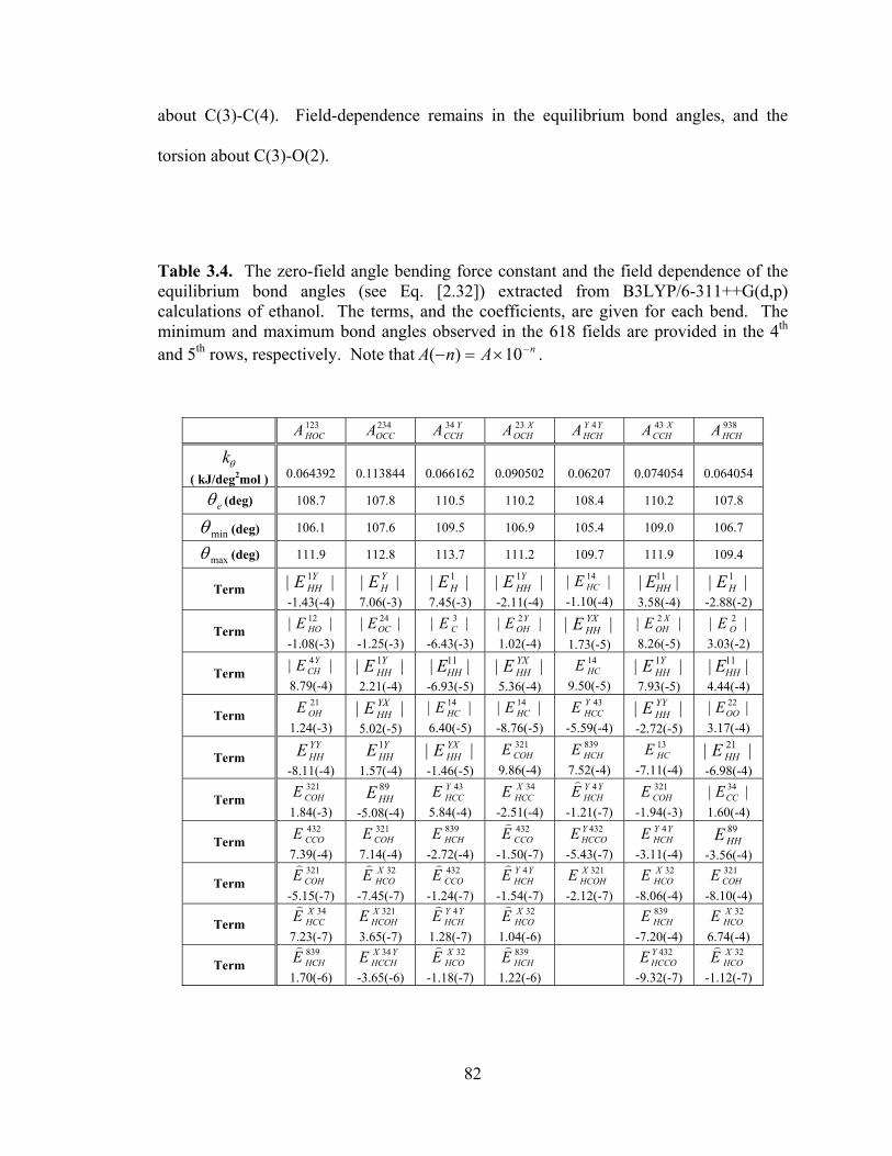
82

about C(3)-C(4). Field-dependence remains in the equilibrium bond angles, and the

torsion about C(3)-O(2).

Table 3.4. The zero-field angle bending force constant and the field dependence of the equilibrium bond angles (see Eq. [2.32]) extracted from B3LYP/6-311++G(d,p) calculations of ethanol. The terms, and the coefficients, are given for each bend. The minimum and maximum bond angles observed in the 618 fields are provided in the 4th and 5th rows, respectively. Note that nAnA −×=− 10)( .

123HOCA 234

OCCA YCCHA 34 X

OCHA 23 YYHCHA 4 X

CCHA 43 938HCHA

θk ( kJ/deg2mol )

0.064392

0.113844

0.066162

0.090502

0.06207

0.074054

0.064054

eθ (deg) 108.7 107.8 110.5 110.2 108.4 110.2 107.8

minθ (deg) 106.1 107.6 109.5 106.9 105.4 109.0 106.7

maxθ (deg) 111.9 112.8 113.7 111.2 109.7 111.9 109.4

Term || 1YHHE

-1.43(-4) || Y

HE 7.06(-3)

|| 1HE

7.45(-3) || 1Y

HHE -2.11(-4)

|| 14HCE

-1.10(-4) || 11

HHE 3.58(-4)

|| 1HE

-2.88(-2)

Term || 12HOE

-1.08(-3) || 24

OCE -1.25(-3)

|| 3CE

-6.43(-3) || 2Y

OHE 1.02(-4)

|| YXHHE

1.73(-5) || 2 X

OHE 8.26(-5)

|| 2OE

3.03(-2)

Term || 4YCHE

8.79(-4) || 1Y

HHE 2.21(-4)

|| 11HHE

-6.93(-5) || YX

HHE 5.36(-4)

14HCE

9.50(-5) || 1Y

HHE 7.93(-5)

|| 11HHE

4.44(-4)

Term 21OHE

1.24(-3) || YX

HHE 5.02(-5)

|| 14HCE

6.40(-5) || 14

HCE -8.76(-5)

43YHCCE

-5.59(-4) || YY

HHE -2.72(-5)

|| 22OOE

3.17(-4)

Term YYHHE

-8.11(-4)

YHHE 1

1.57(-4) || YX

HHE -1.46(-5)

321COHE

9.86(-4)

839HCHE

7.52(-4)

13HCE

-7.11(-4) || 21

HHE -6.98(-4)

Term 321COHE

1.84(-3)

89HHE

-5.08(-4)

43YHCCE

5.84(-4)

34XHCCE

-2.51(-4)

YYHCHE 4)

-1.21(-7)

321COHE

-1.94(-3) || 34

CCE 1.60(-4)

Term 432CCOE

7.39(-4)

321COHE

7.14(-4)

839HCHE

-2.72(-4)

432CCOE)

-1.50(-7)

432YHCCOE

-5.43(-7)

YYHCHE 4

-3.11(-4)

89HHE

-3.56(-4)

Term 321COHE)

-5.15(-7)

32XHCOE)

-7.45(-7)

432CCOE)

-1.24(-7)

YYHCHE 4)

-1.54(-7)

321XHCOHE

-2.12(-7)

32XHCOE

-8.06(-4)

321COHE

-8.10(-4)

Term 34X

HCCE)

7.23(-7)

321XHCOHE

3.65(-7)

YYHCHE 4)

1.28(-7)

32XHCOE)

1.04(-6)

839HCHE

-7.20(-4)

32XHCOE

6.74(-4)

Term 839HCHE)

1.70(-6)

YXHCCHE 34

-3.65(-6)

32XHCOE)

-1.18(-7)

839HCHE)

1.22(-6)

432Y

HCCOE -9.32(-7)

32XHCOE)

-1.12(-7)

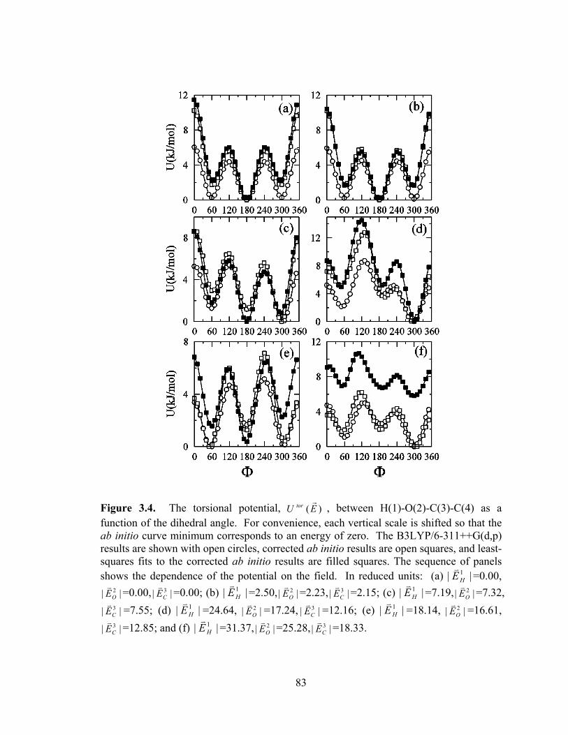
83

Figure 3.4. The torsional potential, )(EU tor

r, between H(1)-O(2)-C(3)-C(4) as a

function of the dihedral angle. For convenience, each vertical scale is shifted so that the ab initio curve minimum corresponds to an energy of zero. The B3LYP/6-311++G(d,p) results are shown with open circles, corrected ab initio results are open squares, and least-squares fits to the corrected ab initio results are filled squares. The sequence of panels shows the dependence of the potential on the field. In reduced units: (a) || 1

HEv

=0.00,|| 2

OEv

=0.00, || 3CEv

=0.00; (b) || 1HEv

=2.50, || 2OEv

=2.23, || 3CEv

=2.15; (c) || 1HEv

=7.19, || 2OEv

=7.32,|| 3

CEv

=7.55; (d) || 1HEv

=24.64, || 2OEv

=17.24, || 3CEv

=12.16; (e) || 1HEv

=18.14, || 2OEv

=16.61,|| 3

CEv

=12.85; and (f) || 1HEv

=31.37, || 2OEv

=25.28, || 3CEv

=18.33.

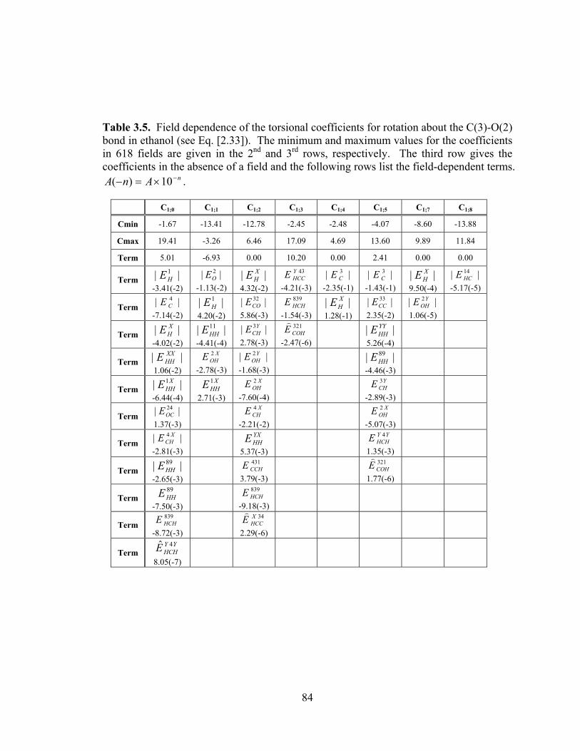
84

Table 3.5. Field dependence of the torsional coefficients for rotation about the C(3)-O(2) bond in ethanol (see Eq. [2.33]). The minimum and maximum values for the coefficients in 618 fields are given in the 2nd and 3rd rows, respectively. The third row gives the coefficients in the absence of a field and the following rows list the field-dependent terms.

nAnA −×=− 10)( .

C1;0 C1;1 C1;2 C1;3 C1;4 C1;5 C1;7 C1;8

Cmin -1.67 -13.41 -12.78 -2.45 -2.48 -4.07 -8.60 -13.88

Cmax 19.41 -3.26 6.46 17.09 4.69 13.60 9.89 11.84

Term 5.01 -6.93 0.00 10.20 0.00 2.41 0.00 0.00

Term || 1HE

-3.41(-2) || 2

OE -1.13(-2)

|| XHE

4.32(-2)

43YHCCE

-4.21(-3) || 3

CE -2.35(-1)

|| 3CE

-1.43(-1) || X

HE 9.50(-4)

|| 14HCE

-5.17(-5)

Term || 4CE

-7.14(-2) || 1

HE 4.20(-2)

|| 32COE

5.86(-3)

839HCHE

-1.54(-3) || X

HE 1.28(-1)

|| 33CCE

2.35(-2) || 2Y

OHE 1.06(-5)

Term || XHE

-4.02(-2) || 11

HHE -4.41(-4)

|| 3YCHE

2.78(-3)

321COHE)

-2.47(-6)

|| YYHHE

5.26(-4)

Term || XXHHE

1.06(-2)

XOHE 2

-2.78(-3) || 2Y

OHE -1.68(-3)

|| 89HHE

-4.46(-3)

Term || 1XHHE

-6.44(-4)

XHHE 1

2.71(-3)

XOHE 2

-7.60(-4)

YCHE 3

-2.89(-3)

Term || 24OCE

1.37(-3)

XCHE 4

-2.21(-2)

XOHE 2

-5.07(-3)

Term || 4 XCHE

-2.81(-3)

YXHHE

5.37(-3)

YYHCHE 4

1.35(-3)

Term || 89HHE

-2.65(-3)

431CCHE

3.79(-3)

321COHE)

1.77(-6)

Term 89HHE

-7.50(-3)

839HCHE

-9.18(-3)

Term 839HCHE

-8.72(-3)

34XHCCE)

2.29(-6)

Term YY

HCHE 4ˆ 8.05(-7)

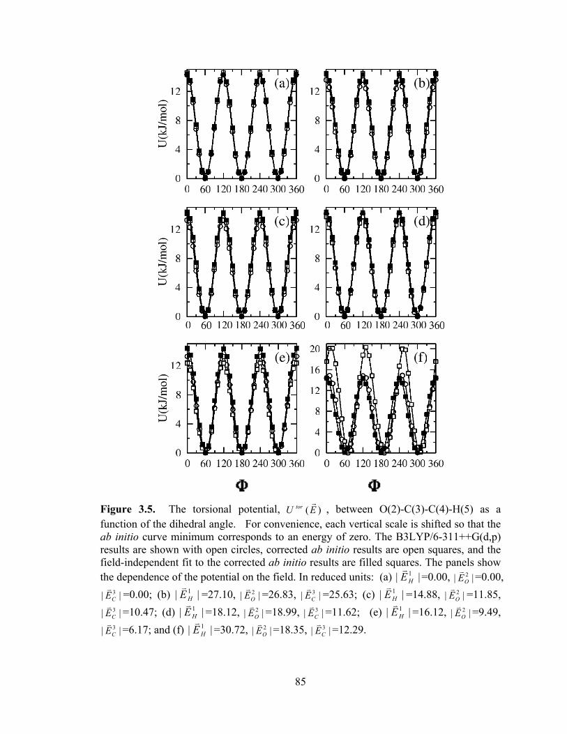
85

Figure 3.5. The torsional potential, )(EU torr

, between O(2)-C(3)-C(4)-H(5) as a function of the dihedral angle. For convenience, each vertical scale is shifted so that the ab initio curve minimum corresponds to an energy of zero. The B3LYP/6-311++G(d,p) results are shown with open circles, corrected ab initio results are open squares, and the field-independent fit to the corrected ab initio results are filled squares. The panels show the dependence of the potential on the field. In reduced units: (a) || 1

HEv

=0.00, || 2OEv

=0.00, || 3

CEv

=0.00; (b) || 1HEv

=27.10, || 2OEv

=26.83, || 3CEv

=25.63; (c) || 1HEv

=14.88, || 2OEv

=11.85, || 3

CEv

=10.47; (d) || 1HEv

=18.12, || 2OEv

=18.99, || 3CEv

=11.62; (e) || 1HEv

=16.12, || 2OEv

=9.49,|| 3

CEv

=6.17; and (f) || 1HEv

=30.72, || 2OEv

=18.35, || 3CEv

=12.29.

86

3.2.6 Simulation details

The canonical (NVT) ensemble is employed for MD simulations of 200 ethanol

molecules, at a density of 0.787 g/cm3 and a temperature of 298 K. Periodic boundary

conditions are employed together with a spherical cut-off for LJ interactions.

The fluid structure is particularly sensitive to the parameters chosen for H(1) and

O(2). This is expected based on the importance of hydrogen bonding in the fluid.

Simulations were performed for 486 models differing in the Lennard-Jones parameters

for O(2) and H(1). Specifically, εo=(0.7, 0.9, 1.1, 1.3, 1.5, 1.7), σo=(0.25, 0.27, 0.29,

0.295, 0.3, 0.305, 0.31, 0.33, 0.35), εH=(0.1, 0.2, 0.3), and σH=(0.02, 0.05, 0.10). We

initially perform 20 ps simulations for the 486 parameter combinations and assess the

fluid structure based on peak positions and coordination numbers, versus neutron

diffraction results[123]. We also require that the charge on O(2) be less than -1.0|e| and

that the diffusion coefficient is within a factor of three of the experimental value[87],

1.2x10-9 m2/s. With these criteria, 25 parameter sets were selected for further

consideration. 50 ps simulations were undertaken for these parameter sets, and the 5 sets

with diffusion coefficients closest to experiment were selected. For the remaining five

models, 1 ns simulations were performed and the final model has been chosen based on

the predicted dielectric constant. Our optimal LJ parameters are given in Table 3.2.

EWALD summations[90], with conducting boundary conditions, are applied for

the long-ranged electrostatic interactions. The additional contributions from the charge

fluctuations are included in the EWALD contribution to the energy by first computing the

EWALD contribution for an atomic fluid and then removing the contribution for the

intramolecular pairs where Eq. [2.26] differs from the point-charge Coulombic potential.

87

For these atomic pairs, the electrostatic energy is calculated from Eq. [2.26]. The results

reported below correspond to a position space cut-off of 26685.0=α Å-1, and a

momentum space cutoff of 272* ≤k .

The procedure employed to generate the starting configuration has been discussed

in detail elsewhere[147]. Briefly, an excess of molecules is placed in the simulation cell

and some are removed at random until the desired number (200) remains. These

molecules are oriented randomly within the simulation cell. Finally, the system is

expanded to reduce any strong repulsions, and Monte Carlo cycles are performed

(assuming that the molecules are rigid and non-polarizable) while the cell is gradually

recompressed to the desired volume. The molecules are then assigned random linear and

angular velocities, consistent with the desired temperature. Following this, the equations

of motion for the charges are equilibrated and the corresponding field-dependent

intramolecular potentials are calculated. In this way, the starting configuration is liquid-

like and each ethanol molecule begins the simulation with distinct intramolecular

potentials and atomic charges.

We compare four different simulations to evaluate the importance of charge

fluctuations and field-dependent intramolecular motion. First, we consider bulk ethanol,

as represented by a non-polarizable flexible molecular model. Second, we allow the

charges to respond to the molecular field but use the zero-field intramolecular potentials.

Third, we consider electric-field dependent charges and intramolecular motion but, in the

evaluation of forces, we treat the intramolecular contribution as though it is field-

independent. With this approximation, the simulation time increases only marginally

while the intramolecular potential still responds to the field. Of course, dynamical

88

motion will not be correct but we explore the accuracy of the equilibrium fluid structure.

Finally, we simulate the full model and include forces due to the field-dependence of the

atomic charges and intramolecular potential.

Nosé-Hoover thermostatting[95, 96] was used to generate canonical averages.

Following Rick et al.[46], extended Lagrangian equations of motion are also applied to

the charges. The relevant conserved quantity in our simulations is shown in Eq. [2.58].

The mass Qm is set to 3 x 10-5 kcal/mol (ps/e)2, a very small value chosen to allow the

atomic charges to rapidly respond to changes in atomic positions. Since these

fluctuations are intended to capture electronic reorganization, it is expected that the

variations in charge should be much faster than atomic motion. Fig. 3.6 shows the impact

of Qm on the fluid structure and diffusion coefficient. The diffusion coefficients in the

figure are evaluated from the slope of the mean square displacement[40] for 20 ps

simulations. The mass chosen in this work is identified by (a) in the figure. From the

figure, the diffusion coefficient’s dependence on the charge mass can be characterized by

a plateau region at very small mass (rapid response region), followed by a sharp peak,

then a drop down to very small values and a gradual rise to the fixed-charge limit.

Clearly, the value of Qm has an important impact on the fluid structure: a very small

value allows the charges to fully respond to changes in nuclear positions, a large value

suppresses the charge fluctuations, but at intermediate values the charges drastically alter

the fluid properties, either by reducing the intermolecular structure, or by greatly

enhancing it. For the simulations Qm must be chosen carefully since an exceedingly

small value will negatively impact the time step of the simulation but a large value will

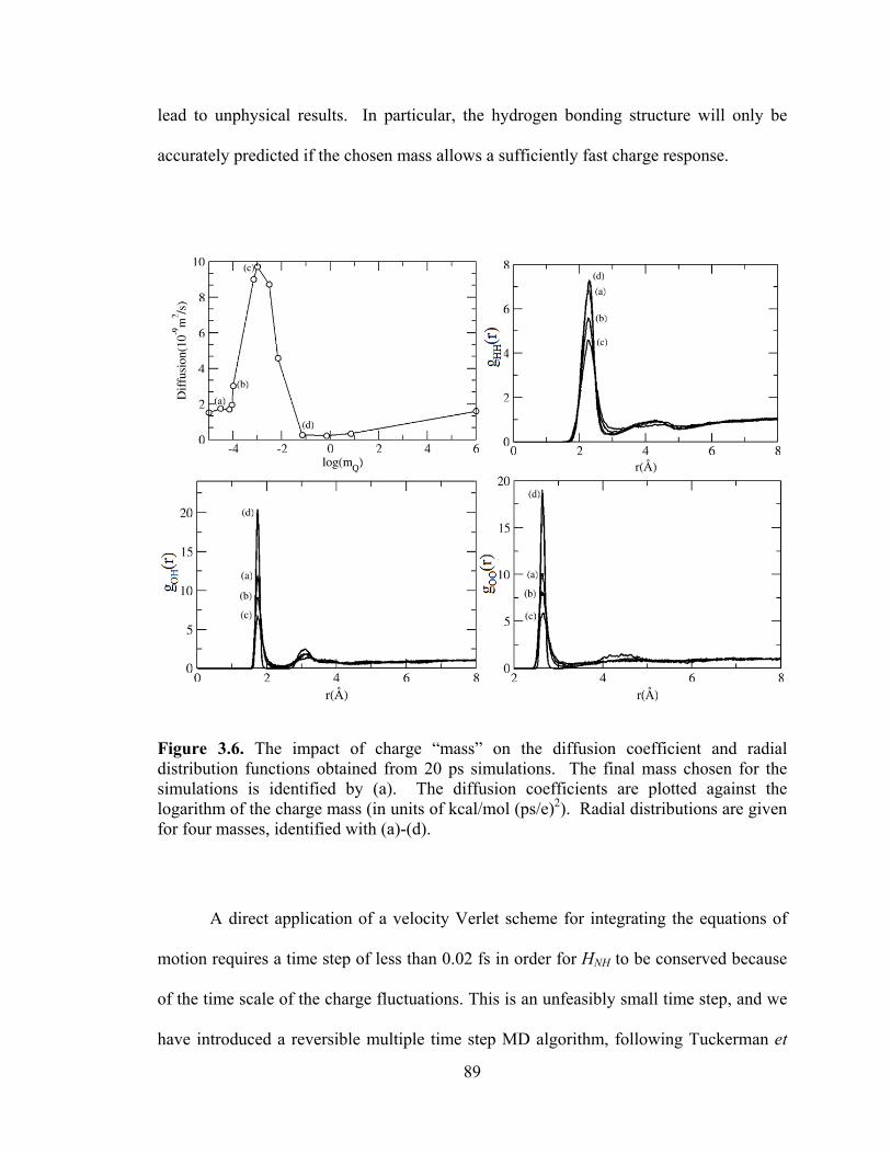
89

lead to unphysical results. In particular, the hydrogen bonding structure will only be

accurately predicted if the chosen mass allows a sufficiently fast charge response.

Figure 3.6. The impact of charge “mass” on the diffusion coefficient and radial distribution functions obtained from 20 ps simulations. The final mass chosen for the simulations is identified by (a). The diffusion coefficients are plotted against the logarithm of the charge mass (in units of kcal/mol (ps/e)2). Radial distributions are given for four masses, identified with (a)-(d).

A direct application of a velocity Verlet scheme for integrating the equations of

motion requires a time step of less than 0.02 fs in order for HNH to be conserved because

of the time scale of the charge fluctuations. This is an unfeasibly small time step, and we

have introduced a reversible multiple time step MD algorithm, following Tuckerman et

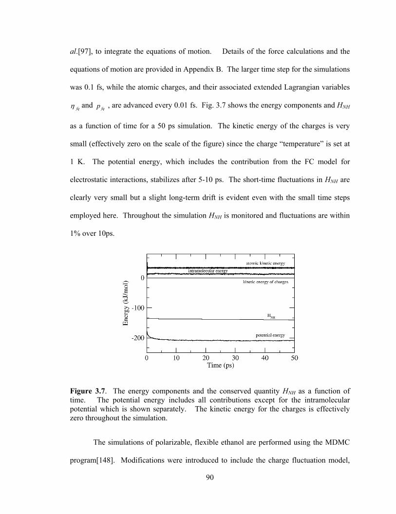
90

al.[97], to integrate the equations of motion. Details of the force calculations and the

equations of motion are provided in Appendix B. The larger time step for the simulations

was 0.1 fs, while the atomic charges, and their associated extended Lagrangian variables

fqη and fqp , are advanced every 0.01 fs. Fig. 3.7 shows the energy components and HNH

as a function of time for a 50 ps simulation. The kinetic energy of the charges is very

small (effectively zero on the scale of the figure) since the charge “temperature” is set at

1 K. The potential energy, which includes the contribution from the FC model for

electrostatic interactions, stabilizes after 5-10 ps. The short-time fluctuations in HNH are

clearly very small but a slight long-term drift is evident even with the small time steps

employed here. Throughout the simulation HNH is monitored and fluctuations are within

1% over 10ps.

Figure 3.7. The energy components and the conserved quantity HNH as a function of time. The potential energy includes all contributions except for the intramolecular potential which is shown separately. The kinetic energy for the charges is effectively zero throughout the simulation.

The simulations of polarizable, flexible ethanol are performed using the MDMC

program[148]. Modifications were introduced to include the charge fluctuation model,

91

the field-dependent intramolecular potential, and the multiple time step algorithm. The

evaluation of forces from the field-dependent intramolecular potential is, by far, the most

time-consuming aspect of the computation (see Appendix B). We have parallelized this

segment of the code to allow for rapid computation of the forces.

In the simulations, it is possible for atoms to experience fields for which the

parameters in Eqs. [2.31]-[2.33] are outside of the range used in building their field-

dependent forms. Although this is a rare event, and the model may perform well in such a

field, we have chosen to introduce a damping function for each parameter in Eqs. [2.31]-

[2.33]. Specifically, we consider the fitted parameters, and extract the minimum and

maximum values observed in the 618 fields. These values are given in Tables 3.3-3.5.

The damped value, xDamp , of a parameter x is obtained from

4/)(minmaxmin

2minmax

2xxae

xxx −−−

+ ( minxx ≤ ) [3.5]

4/)(minmax)(min

2minmax

2min

2)( xxaxxa e

xxexxx −−−− −

+−− (2

maxminmin

xxxx

+≤< ) [3.6]

4/)(minmax)(max

2minmax

2max

2)( xxaxxa e

xxexxx −−−− −

−−+ ( maxmaxmin

2xx

xx≤<

+) [3.7]

4/)(minmaxmax

2minmax

2xxae

xxx −−−

− ( xx <max ) [3.8]

where xmin and xmax are the minimum and maximum values of the parameter, respectively.

Away from the minimum and maximum values, the damping has a negligible effect. The

last term in Eqs. [3.6] and [3.7] is present to ensure continuity of the damped function,

and its slope, at the midpoint value of the parameter range. To evaluate the constant a in

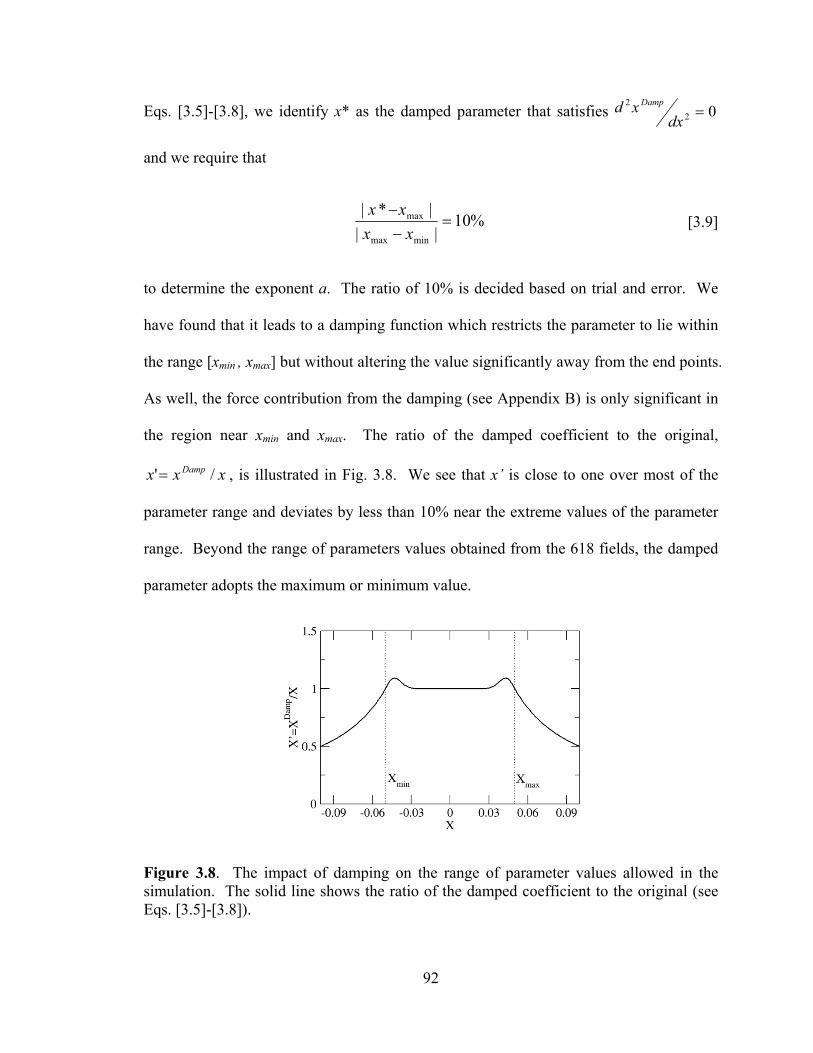
92

Eqs. [3.5]-[3.8], we identify x* as the damped parameter that satisfies 022

=dxxd Damp

and we require that

%10||

|*|

minmax

max =−−

xxxx

[3.9]

to determine the exponent a. The ratio of 10% is decided based on trial and error. We

have found that it leads to a damping function which restricts the parameter to lie within

the range [xmin , xmax] but without altering the value significantly away from the end points.

As well, the force contribution from the damping (see Appendix B) is only significant in

the region near xmin and xmax. The ratio of the damped coefficient to the original,

xxx Damp /'= , is illustrated in Fig. 3.8. We see that x’ is close to one over most of the

parameter range and deviates by less than 10% near the extreme values of the parameter

range. Beyond the range of parameters values obtained from the 618 fields, the damped

parameter adopts the maximum or minimum value.

Figure 3.8. The impact of damping on the range of parameter values allowed in the simulation. The solid line shows the ratio of the damped coefficient to the original (see Eqs. [3.5]-[3.8]).

93

3.3. Results and discussion

In this section, we examine the fluid structure in bulk ethanol. First, we compare

our results to experiment and to those of other ethanol models, then we turn to the

hydrogen-bonding structure in the bulk.

3.3.1 Bulk ethanol

Fig. 3.9 compares radial distributions from the fCINTRA model, from neutron

diffraction[123], and from the non-polarizable OPLS model [127]. The distribution

between hydrogen-bonding hydrogens (H(1) in Fig. 2.8) is shown in the top-panel. The

first peak in the experimental distribution is relatively broad and all models we have

examined (both polarizable and non-polarizable) have narrower peaks. Given this, we

have chosen to optimize our model based on the coordination number and peak position.

Coordination number is the total number of neighbors around a central atom and can be

obtained by integrating over the first peak of the radial distribution [42]. As shown in

Table 3.6, these are well reproduced with the fCINTRA model. The small secondary

peak in gHH(r), at r ≈ 4.3 Å, is also well-reproduced by the fCINTRA model. In contrast,

the OPLS model places this peak at too large a separation and underestimates the

coordination number.

The second distribution, gXH(r), is a combination from the O(2)-H(1), C(3)-H(1),

and C(4)-H(1) interatomic pairs. The neutron diffraction experiments[123] were not able

to separate these contributions, and the combination in Fig. 3.9 is

gXH(r) =0.303 gH(1)O(2) (r) +0.349 gH(1)C(3) (r) +0.349 gH(1)C(4) (r). [3.10]

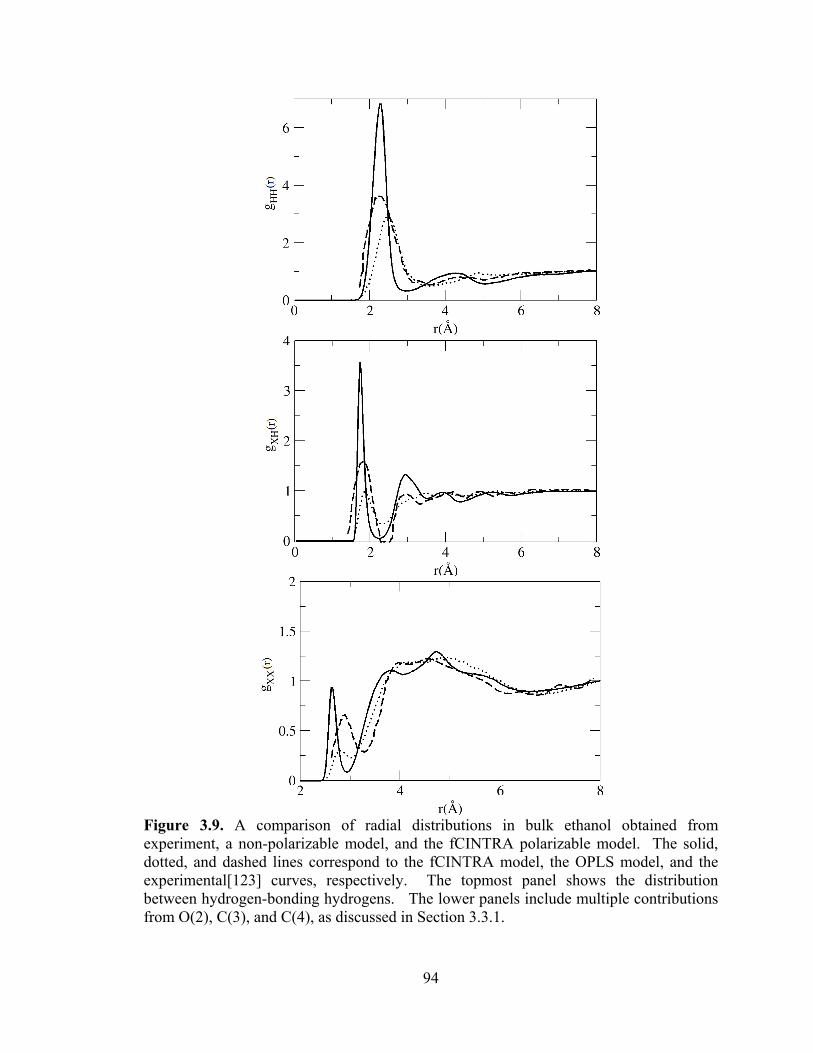
94

Figure 3.9. A comparison of radial distributions in bulk ethanol obtained from experiment, a non-polarizable model, and the fCINTRA polarizable model. The solid, dotted, and dashed lines correspond to the fCINTRA model, the OPLS model, and the experimental[123] curves, respectively. The topmost panel shows the distribution between hydrogen-bonding hydrogens. The lower panels include multiple contributions from O(2), C(3), and C(4), as discussed in Section 3.3.1.

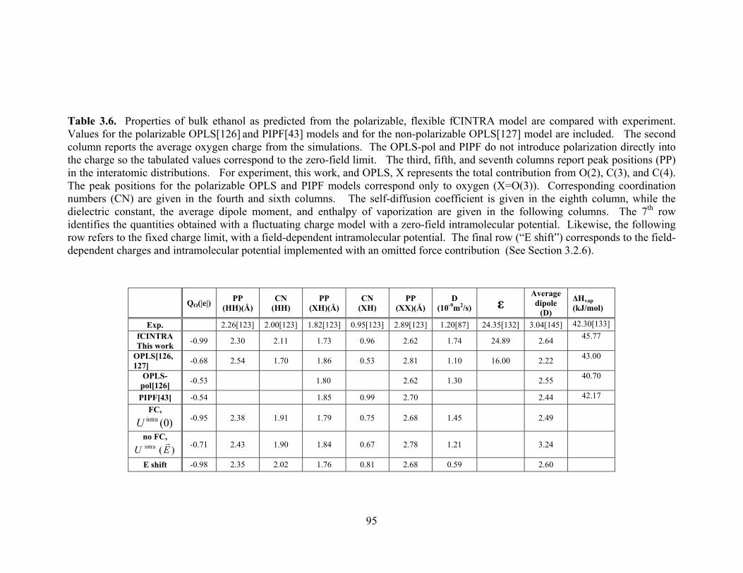
95

Table 3.6. Properties of bulk ethanol as predicted from the polarizable, flexible fCINTRA model are compared with experiment. Values for the polarizable OPLS[126] and PIPF[43] models and for the non-polarizable OPLS[127] model are included. The second column reports the average oxygen charge from the simulations. The OPLS-pol and PIPF do not introduce polarization directly into the charge so the tabulated values correspond to the zero-field limit. The third, fifth, and seventh columns report peak positions (PP) in the interatomic distributions. For experiment, this work, and OPLS, X represents the total contribution from O(2), C(3), and C(4). The peak positions for the polarizable OPLS and PIPF models correspond only to oxygen (X=O(3)). Corresponding coordination numbers (CN) are given in the fourth and sixth columns. The self-diffusion coefficient is given in the eighth column, while the dielectric constant, the average dipole moment, and enthalpy of vaporization are given in the following columns. The 7th row identifies the quantities obtained with a fluctuating charge model with a zero-field intramolecular potential. Likewise, the following row refers to the fixed charge limit, with a field-dependent intramolecular potential. The final row (“E shift”) corresponds to the field-dependent charges and intramolecular potential implemented with an omitted force contribution (See Section 3.2.6).

QO(|e|) PP (HH)(Å)

CN (HH)

PP (XH)(Å)

CN (XH)

PP (XX)(Å)

D (10-9m2/s) ε

Average dipole

(D)

ΔHvap (kJ/mol)

Exp. 2.26[123] 2.00[123] 1.82[123] 0.95[123] 2.89[123] 1.20[87] 24.35[132] 3.04[145] 42.30[133] fCINTRA This work -0.99 2.30 2.11 1.73 0.96 2.62 1.74 24.89 2.64 45.77

OPLS[126, 127] -0.68 2.54 1.70 1.86 0.53 2.81 1.10 16.00 2.22 43.00

OPLS-pol[126] -0.53 1.80 2.62 1.30 2.55 40.70

PIPF[43] -0.54 1.85 0.99 2.70 2.44 42.17

FC,

)0(intraU -0.95 2.38 1.91 1.79 0.75 2.68 1.45 2.49

no FC, )(intra EUr

-0.71 2.43 1.90 1.84 0.67 2.78 1.21 3.24

E shift -0.98 2.35 2.02 1.76 0.81 2.68 0.59 2.60

96

As shown in Fig. 3.9 and Table 3.6, the fCINTRA model reproduces the first peak

position and coordination number but is much sharper than the experimental curve.

Following the initial peak, due almost entirely to oxygen, the experiments indicate an

oscillatory behavior due to contributions from all three atoms. Our polarizable model

also shows oscillatory behavior and reproduces the second peak position accurately but

the third peak is shifted to smaller separations. The OPLS curve shows far less structure

than either the experiment or the fCINTRA distributions and the coordination number is

underestimated by roughly 40%.

The final distribution in Fig. 3.9, gXX(r), includes a contribution from several

atom pairs, as follows

gXX (r) =0.0924 gO(2)O(2)(r)+0.212 gC(3)O(2)(r)+0.121 gC(3)C(3)(r)+0.212 gC(4)O(2)(r)+

0.242 gC(4)C(3)(r)+0.121 gC(4)C(4) (r) [3.11]

Benmore et al.[123] note concerns about contributions from hydrogens remaining in this

distribution. As a result, we have opted to focus on overall agreement between

experiment and theory for this particular distribution. We find that the position and

intensity of the first peak is highly variable. Our final parameters (in Table 3.2) give a

peak that appears at smaller separations relative to experiment but the area under this

peak is reasonable. The broad secondary structure is also sensitive to model details but,

as shown in Fig. 3.9, the fCINTRA model shows the expected double peak followed by a

broad shoulder.

Table 3.6 provides a comparison of the properties predicted from the fCINTRA

model, from experiment, from the non-polarizable OPLS model, and for two polarizable

models. Consider first the charge on O(2). The OPLS-pol and PIPF models do not

97

include the polarizability directly into the charges. The PIPF model, for example,

introduces atomic dipoles to represent the polarizability. However, the static charges

employed in these simulations are significantly smaller than the gas phase charge (Table

3.2). The average charges obtained in this work are fairly large but we note parameter

sets that gave smaller average charges inevitably led to a high diffusion coefficient and

low coordination numbers.

Self-diffusion is overestimated by the fCINTRA model. However, as shown in

Fig. 3.6, the diffusion coefficient is highly sensitive to the mass associated with charge

fluctuations. Fig. 3.6 suggests that a further reduction in the mass would decrease the

diffusion coefficient slightly but the final value would still lie above the experimental

value.

The fCINTRA model predicts a dielectric constant, ε, in very close agreement

with experiment. The dielectric constant is calculated from[149]:

)||||(3

4 22 ><−><+= ∞ MMTVkb

rrπεε [3.12]

where Mr

is the total dipole moment of the simulation box:

∑∑= =

=M N

iii rQM

1 1ααα

α rr [3.13]

Over the course of the simulation <| Mr

|> should average to zero and we monitor this

quantity as a measure of the convergence of the dielectric. The value given in Table 3.6

includes the contribution from <| Mr

|>2 , although it should be strictly zero, and it is less

than 1% of the reported dielectric constant. In Eq. [3.12], ∞ε is calculated from the

Clausius-Mossotti equation[150]:

98

vαπ

εε

34

21=

+−

∞

∞ [3.14]

where α is the molecular polarizability (see Appendix A) and v is the molecular volume.

The fCINTRA model predicts ∞ε to be 1.88, which is quite close to the experiment

value[132] of 1.93.

The average dipole moment and the enthalpy of vaporization, ΔHvap, are evaluated

from the simulations but are not considered in the parameter selection. Relative to the

non-polarizable OPLS and the polarizable models, the fCINTRA model predicts the

average dipole in closest agreement with experiment although the experimental value is

still underestimated by 13%. The distribution of molecular dipole moments is a Gaussian

for the fCINTRA model with a standard deviation of 0.308D. The evaluation of the

enthalpy of vaporization proceeds as discussed elsewhere[43]. Briefly, ΔHvap is evaluated

from

ΔHvap = [Eintra(g)-Ei(l)-Eintra(l)] + RT - (Ho- H) [3.15]

where Ho- H is obtained from experiment[127]. The calculation of the average gas phase

intramolecular energy, Eintra(g), proceeds by simulating a “fluid” in which all the

intermolecular interactions are omitted. In other words, individual molecules are flexible

and polarizable but no longer interact in the fluid. The equations of motion are integrated

as discussed in Section 2.4, except that Nosé-Hoover chains[81] are implemented to

ensure proper canonical averages. From Table 3.6, the fCINTRA model predicts a

vaporization enthalpy in good agreement with experiment, although the experimental

value is exceeded by 8%.

99

The last three rows in Table 3.6 show the properties from sub-models

corresponding to simplified versions of the fCINTRA model. All three models result in

simulations that are comparable, time-wise, to those for non-polarizable models. The use

of the FC model, with zero-field intramolecular potentials, leads to properties that are in

reasonable agreement with experiment although the coordination numbers and the

average dipole are consistently too small. The use of field-dependent intramolecular

potentials with fixed-charges also reduces the coordination numbers and average dipole.

In this case, the dipole distribution is bimodal with a peak at 2.34D and a peak at 3.80D.

The “E shift” method, in which the forces due to the field-dependence of the

intramolecular coefficients (the last term in Eq. [B1]) are neglected, yields a diffusion

coefficient that is far too small. This suggests that the coupling term cannot be omitted.

Overall, the fCINTRA model compares favorably with experiment and other

polarizable models. The introduction of field-dependence in the charges and the

intramolecular potentials leads to accurate predictions for a range of properties including

the fluid structure, the diffusion coefficient, the dielectric, the average dipole, and the

enthalpy of vaporization. Further model refinement would undoubtedly improve the

agreement with experiment. Such improvements would include optimization of all the LJ

parameters, further minimization of the charge mass, and perhaps inclusion of field-

dependence in all the intramolecular parameters. The limit on the maximum oxygen

charge could also be relaxed. The latter may lead to an increase in the average dipole and

a decrease in the self-diffusion coefficient, but may adversely impact the dielectric

constant and vaporization enthalpy.

100

3.3.2 Hydrogen bonding

Fig. 3.10 shows three snapshots of the fluid. The left-most panel shows alkyl rich

regions with a “loose” hydrogen bonding network separating the regions. Consider the

central panel where O(2) and H(1) are emphasized. From the figure, the hydrogen

bonding network in the fluid consists of complex chain-like structures. In order to

quantify this network, we apply a stringent structural definition of the hydrogen-

bond[120]: rHO < 2.6 Å, rOO < 3.5 Å, and the O-H-O angle is greater than 150 degrees.

Using this definition, snapshots have been analyzed to ascertain the hydrogen bond

characteristics and the results are collected in Table 3.7. For the fCINTRA model, the

average chain length includes roughly 24 molecules. A branch, in which an ethanol

molecule hydrogen bonds to three others, occurs on average once or twice every chain.

As well, only 1% of the molecules are not participating in a hydrogen-bond at any given

time. The statistics collected for the non-polarizable OPLS model show a drastically

reduced chain length, with a commensurate increase in the percentage of single

molecules. Thus, this nonpolarizable model greatly underestimates the extent and

character of hydrogen-bonding in the fluid. The statistics for the “partial” models are

also given in Table 3.7. In all cases, the length of the hydrogen bonding chains has

decreased. Overall, the FC model with zero-field intramolecular potentials is superior to

the other sub-models.

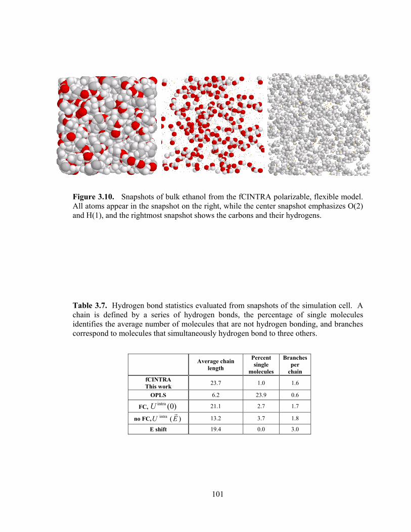
101

Figure 3.10. Snapshots of bulk ethanol from the fCINTRA polarizable, flexible model. All atoms appear in the snapshot on the right, while the center snapshot emphasizes O(2) and H(1), and the rightmost snapshot shows the carbons and their hydrogens.

Table 3.7. Hydrogen bond statistics evaluated from snapshots of the simulation cell. A chain is defined by a series of hydrogen bonds, the percentage of single molecules identifies the average number of molecules that are not hydrogen bonding, and branches correspond to molecules that simultaneously hydrogen bond to three others.

Average chain length

Percent single

molecules

Branches per

chain fCINTRA This work 23.7 1.0 1.6

OPLS 6.2 23.9 0.6

FC, )0(intraU 21.1 2.7 1.7

no FC, )(intra EUr

13.2 3.7 1.8

E shift 19.4 0.0 3.0

102

3.4. Conclusions

In this chapter, we have developed a polarizable and flexible model for ethanol.

Our approach differs from others[43, 45, 46, 126, 127] in that we allow the

intramolecular potential to vary with the field. Atomic charges also fluctuate with the

field according to the FC method[46]. At any instant in time, each ethanol molecule in

the bulk has a unique set of atomic charges, and its own set of intramolecular potentials.

The idea here is that, for each molecule, the electron distribution is unique and leads to

distinct atomic charges and intramolecular potentials.

The model we have developed relies heavily on ab initio calculations, and we

begin with benchmarking of density functionals and basis sets. As well, we collect

information on the fields typically experienced by ethanol molecules in the bulk.

Following this, an extensive series of B3LYP/6-311++G(d,p) calculations of ethanol, in

the presence of 618 fields, is undertaken to develop field-dependent intramolecular

potentials. The final ethanol model is obtained by comparison with interatomic

distributions[123] and other properties. Although the distribution functions available

for comparison are not fully resolved, we find that they do provide a sensitive test of our

models. In the end, only four Lennard-Jones parameters are chosen by direct comparison

with experiment. In particular, the fluid structure is highly sensitive to the LJ parameters

on O(2) and H(1) and small changes in the parameters change the H-bonding in the fluid

and lead to significant differences in interatomic distributions.

The stretching and bending motion in ethanol is not strongly field-dependent, and

we have chosen to introduce field dependence in only the equilibrium bond angles,

leaving the equilibrium bond lengths and the force constants field-independent. On the

103

other hand, the torsional potential for rotation about the C(3)-O(2) bond, which governs

the position of the H-bonding hydrogen, is strongly field-dependent. In some fields, this

torsional potential is highly asymmetric, and the global minimum is not at the zero-field

value of 180 degrees. An analysis of hydrogen bond characteristics shows that the

fCINTRA model predicts longer chains of H-bonded molecules, with very few branching

events and few isolated molecules. Other models underestimate the chain lengths and

overestimate the fraction of non H-bonding molecules. The fCINTRA model allows the

hydrogen to reposition itself in response to the field, thereby optimizing the hydrogen-

bond network.

We have analyzed the impact of field-sensitivity of the model by performing a

series of simulations on sub-models of fCINTRA. First, the fluid in which the

intramolecular potential is field-independent but the charges respond to the field is

considered. This model compares favorably with the fCINTRA model although, on

average, the hydrogen bonded chains are shorter and the average dipole has been

lowered. Second, the intramolecular potential changes with the field, but the atomic

charges do not vary. Table 3.6 suggests that this model compares favorably with

experiment. However, the model yields a bimodal dipole distribution and the average

length for hydrogen-bonded chains is much shorter than for fCINTRA. Finally, both the

charges and the intramolecular potential vary but some force terms are omitted. This

approach yields a diffusion coefficient well below experiment. Overall, the sub-model in

which only the charges fluctuate compares best with fCINTRA.

The implementation of the fCINTRA model presents several challenges. First,

the evaluation of the field-dependent intramolecular potential parameters must be

104

efficient. We have chosen to expand the coefficients into field-analogs of structural

quantities. We have also been careful to enforce any expected symmetries in the

coefficients. Second, the FC method has only been applied in a few instances[46, 50, 53,

55, 131] and we have found that the simulations are highly sensitive to the choice of

charge “mass” and to the definition of the Coulomb overlap. For the latter, we employed

a simple interpolation of numerically integrated overlaps(Eq. [2.27]) that was accurate,

stable, and efficient (See Section 2.2.1). Third, within the simulations, the molecules

experience a range of fields and some of these may lead to intramolecular potential

coefficients that lie outside of the range used in the parameterization of the model. We

have dealt with this by introducing a damping function that constrains the coefficients to

within the interval. Fourth, the charges may “heat up” during the simulation, but we have

implemented a Nosé-Hoover thermostat to constrain their temperature to 1K. Finally, the

time required for charge fluctuations must be much shorter than for nuclear motion. As a

result, a multiple time-step molecular dynamics algorithm is also required.

The polarizable model methodology developed in this chapter offers a viable

alternative to ab initio simulations. Although the model development requires a large

number of initial ab initio calculations, the individual calculations are fast. As well, the

simulations are far less demanding than full ab initio simulations although they are much

more time-consuming than for non-polarizable models. In particular, nanosecond

simulations are still feasible with the methodology developed in this chapter.

105

Chapter 4 Chirality transfer: The impact of a chiral solute on an achiral solvent In this chapter, the chirality transfer from chiral solutes to achiral solvents is

discussed. The study is based on MD simulations of two solvents, which are ethanol and

benzyl alcohol, and three solutes, which are PAMD, styrene oxide and acenaphthenol.

The induced chirality is quantified by a chirality index and the spatial characteristics of

the chirality transfer are analyzed.

4.1. Introduction

The impact of solvent on the properties of chiral solutes has been studied in some

detail using spectroscopy [24, 30, 31]. Recently, experimental studies have begun to

focus on the chirality present in the solvent when it surrounds a chiral solute [26-29].

The chirality transfer from a chiral solute to an achiral solvent, in the isotropic

phase, is the focus of this chapter. To our knowledge, this is the first detailed simulation

study of chirality transfer in isotropic fluids. With this in mind, we assess the structural

chirality introduced in the solvent molecules rather than emphasizing a particular

property (such as VCD or ORD spectra). This is accomplished with molecular dynamics

(MD) simulations of a small number of chiral solutes surrounded by solvent, and the

chirality induced in the solvent molecules is assessed via the long-time average of a

chirality index. A chirality index proposed by Osipov et al.[66] has been chosen for the

present work since it can be readily evaluated and satisfies all the requirements noted in

106

Section 1.4. In this chapter, the Osipov index is evaluated for all solvents in the vicinity

of the chiral solute (within 15 Å of specified solute atoms). The excess solvent chirality,

as represented by the long-time average of the Osipov chirality index, is evaluated and

categorized based on the solvent position about the solute.

In docking processes, including selectivity in chiral chromatography[151-153]

and lock-and-key mechanisms in biology,[154, 155] three-point recognition models are

often assumed. Here, hydrogen bonding and π-π interactions between aromatic groups

are usually present in the recognition models. By analogy with these models, we assume

that such interactions also play an important role in the chirality transfer process. To

study the impact of these interactions in more detail, we examine two solvents: Ethanol

and benzyl alcohol. The former will interact with the chiral solute primarily via a

hydrogen bond while the latter can simultaneously form a π- π interaction and a hydrogen

bond. Three solutes have been considered: Styrene oxide, acenaphthenol, and n-(1-(4-

bromophenyl)ethyl)pivalamide (PAMD). Styrene oxide is small, compact, and accessible

to the solvent from all sides. Acenaphthenol is larger, but conformationally restricted.

PAMD has multiple functional groups, a more complex structure, and many conformers.

A comparison between these solutes will provide some indication of the relationship

between the chirality transfer and the solute size and properties. We also examine the

impact of conformational averaging by comparing the excess solvent chirality about rigid

and flexible PAMD.

The MD simulations provide insights into the magnitude and characteristics of the

chirality transfer between a chiral solute and its surrounding solvent. However, the level

of solvent representation is important for an exploration of chirality transfer. In typical

107

MD simulations, the molecules are nonpolarizable and the instantaneous molecular

environment does not impact any of the parameters defining the molecular force field.

The importance of polarizability has been explored for small solvents, including water[44,

46, 47, 130] and alcohols[43, 45, 91, 126], during the past decade. These studies show

that the fluid structure, in particular the hydrogen bonding network, is impacted by the

response of the molecules to their environment. The relationship between solvent

polarizability and chirality transfer is examined here, with the expectation that a

polarizable solvent will respond more effectively to a chiral environment, as discussed in

Chapter 3 [91]. Several polarizable models for ethanol have been reported [43, 45, 91,

126], but in most cases the molecular flexibility parameters (intramolecular potential) are

unchanged by the local environment. Polarizability is included via variations in atomic

charges, multipole moments, or by the addition of atomic dipoles. In Chapter 3,[91] we

discussed a polarizable ethanol model that allows for fluctuating atomic charges and

intramolecular potentials that are field dependent. In this chapter, we explore the impact

of solvent representation by evaluating chirality transfer for a fully nonpolarizable

solvent, a partially polarizable solvent (atomic charge fluctuations only), and a fully

polarizable solvent. We find that chirality transfer is greatly underestimated without

allowance for solvent polarization.

In section 4.4.2, we briefly discuss the solvent models, the inclusion of

polarizability, the chiral index, and the simulation details. Results from extensive MD

simulations are reported in Section 4.4.3 and brief conclusions are presented in Section

4.4.4.

108

4.2. Methods

4.2.1 Solvent and solute models

The fully polarizable fluctuating charge and intramolecular potential (fCINTRA)

model for ethanol is discussed in detail in Chapter 3. In this section, we begin by briefly

describing the molecular potentials used to represent benzyl alcohol. The solvents and

solutes are shown in Fig. 4.1 along with the atom numbering used throughout this

chapter. For benzyl alcohol, a fully polarizable solvent model is not available. We have

proceeded to develop a partially polarizable model as follows. First, we employ OPLS

parameters[156] for the LJ potential in Eq. [2.12]. For the intramolecular potential, an

extensive series of B3LYP/6-311G(d,p) ab initio calculations have been performed.

Since the aromatic ring is very rigid, only 5 stretches, 9 bends, 2 torsions, and 1 improper

torsion are chosen to represent the molecular flexibility. The potential parameters,

obtained by least squares fits to the ab initio calculations, are given in Table 4.1. Each

stretching force constant is extracted from nine energy calculations, as the bond is

compressed and stretched away from the equilibrium value. Bending potentials are

obtained by least squares fits to nine energy calculations where the angle is varied within

sixteen degrees of the equilibrium value. For torsion potentials, the angle is varied from

0 to 360o, in steps of 10o. The improper torsion potential about C(6) is obtained from

nine restricted geometry optimizations as C(6) is raised above and below the plane of the

neighboring three atoms.

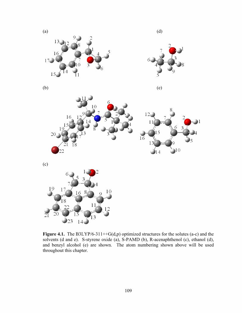
109

(a) (d)

(b) (e)

(c)

Figure 4.1. The B3LYP/6-311++G(d,p) optimized structures for the solutes (a-c) and the solvents (d and e). S-styrene oxide (a), S-PAMD (b), R-acenaphthenol (c), ethanol (d), and benzyl alcohol (e) are shown. The atom numbering shown above will be used throughout this chapter.

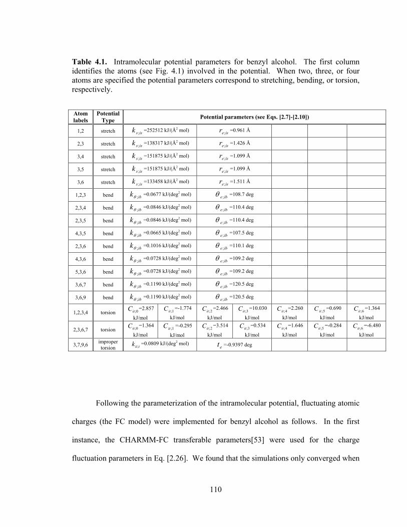
110

Table 4.1. Intramolecular potential parameters for benzyl alcohol. The first column identifies the atoms (see Fig. 4.1) involved in the potential. When two, three, or four atoms are specified the potential parameters correspond to stretching, bending, or torsion, respectively.

Atom labels

Potential Type Potential parameters (see Eqs. [2.7]-[2.10])

1,2 stretch issk ; =252512 kJ/(Å2 mol) iser ; =0.961 Å

2,3 stretch issk ; =138317 kJ/(Å2 mol) iser ; =1.426 Å

3,4 stretch issk ; =151875 kJ/(Å2 mol) iser ; =1.099 Å

3,5 stretch issk ; =151875 kJ/(Å2 mol) iser ; =1.099 Å

3,6 stretch issk ; =133458 kJ/(Å2 mol) iser ; =1.511 Å

1,2,3 bend ibk ;θ =0.0677 kJ/(deg2 mol) ibe ;θ =108.7 deg

2,3,4 bend ibk ;θ =0.0846 kJ/(deg2 mol) ibe ;θ =110.4 deg

2,3,5 bend ibk ;θ =0.0846 kJ/(deg2 mol) ibe ;θ =110.4 deg

4,3,5 bend ibk ;θ =0.0665 kJ/(deg2 mol) ibe ;θ =107.5 deg

2,3,6 bend ibk ;θ =0.1016 kJ/(deg2 mol) ibe ;θ =110.1 deg

4,3,6 bend ibk ;θ =0.0728 kJ/(deg2 mol) ibe ;θ =109.2 deg

5,3,6 bend ibk ;θ =0.0728 kJ/(deg2 mol) ibe ;θ =109.2 deg

3,6,7 bend ibk ;θ =0.1190 kJ/(deg2 mol) ibe ;θ =120.5 deg

3,6,9 bend ibk ;θ =0.1190 kJ/(deg2 mol) ibe ;θ =120.5 deg

1,2,3,4 torsion =2.857

kJ/mol 1;itC =-1.774

kJ/mol

=2.466

kJ/mol

=10.030

kJ/mol 4;itC =2.260

kJ/mol 5;itC =0.690

kJ/mol 6;itC =1.364

kJ/mol

2,3,6,7 torsion =1.364

kJ/mol 1;itC =-0.295

kJ/mol

=3.514

kJ/mol

=0.534

kJ/mol 4;itC =1.646

kJ/mol 5;itC =-0.284

kJ/mol 6;itC =-6.480

kJ/mol

3,7,9,6 improper torsion tiik ;

=0.0809 kJ/(deg2 mol) et =-0.9397 deg

Following the parameterization of the intramolecular potential, fluctuating atomic

charges (the FC model) were implemented for benzyl alcohol as follows. In the first

instance, the CHARMM-FC transferable parameters[53] were used for the charge

fluctuation parameters in Eq. [2.26]. We found that the simulations only converged when

0;itC 2;itC 3;itC

0;itC 2;itC 3;itC

111

the “mass” governing charge fluctuation was 7x10-3 kcal/mol (ps2/e2) or larger. In

practice, this mass must be small enough to allow rapid charge fluctuation in response to

molecular motion. Unfortunately, the mass required for benzyl alcohol was large and we

found that the average charge on C(3) was unphysical. We proceeded to develop charge-

fluctuation parameters specifically for benzyl alcohol, following the methodology

discussed in Appendix A. adopted previously for ethanol [91]. Briefly, the atomic

charges, as evaluated from the CHELPG[110] algorithm applied to B3LYP calculations

with the 6-311++G(d,p) basis set, were obtained when the molecule was placed in 30

diverse fields. Based on the fitting of the molecular response, parameters for Eq. [2.26]

were extracted. With the new parameters, convergence was achieved for a “mass” as low

as 5x10-5 kcal/mol (ps2/e2) and the corresponding atomic charges were reasonable. Table

4.2 presents the fluctuating charge parameters for benzyl alcohol. It is interesting to note

that the atomic electronegativities derived specifically for benzyl alcohol were

consistently larger than the transferrable CHARMM-FC values. The resulting benzyl

alcohol model gives a self diffusion coefficient of 4.27 x 10-12 m2/s, a dielectric constant

of 12.13, and a dipole polarizability of 14.67 Å3. These values are in good agreement

with the corresponding experimental values of 4.01 x 10-12 m2/s [157], 12.5 (estimated

from measured dielectric constants at 20oC and 30oC [158]), and 12.87 Å3 [159, 160],

respectively.

The molecular models employed for styrene oxide and PAMD have been

described elsewhere [113, 161]. Here we note that these solutes are represented by

flexible and nonpolarizable models and that the rings are kept rigid during the

simulations, as is also done for benzyl alcohol and acenaphthenol. That is, the ring atoms

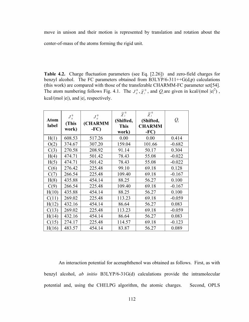
112

move in unison and their motion is represented by translation and rotation about the

center-of-mass of the atoms forming the rigid unit.

Table 4.2. Charge fluctuation parameters (see Eq. [2.26]) and zero-field charges for benzyl alcohol. The FC parameters obtained from B3LYP/6-311++G(d,p) calculations (this work) are compared with those of the transferable CHARMM-FC parameter set[54]. The atom numbering follows Fig. 4.1. The 0

iiJ , 0~iχ , and iQ are given in kcal/(mol |e|2) ,

kcal/(mol |e|), and |e|, respectively.

Atom label

0iiJ

(This work)

0iiJ

(CHARMM-FC)

0~iχ

(Shifted, This

work)

0~iχ

(Shifted, CHARMM

-FC)

iQ

H(1) 608.53 517.26 0.00 0.00 0.414 O(2) 374.67 307.20 159.04 101.66 -0.682 C(3) 270.58 208.92 91.14 50.17 0.304 H(4) 474.71 501.42 78.43 55.08 -0.022 H(5) 474.71 501.42 78.43 55.08 -0.022 C(6) 276.42 225.48 99.10 69.18 0.128 C(7) 266.54 225.48 109.40 69.18 -0.167 H(8) 435.88 454.14 88.25 56.27 0.100 C(9) 266.54 225.48 109.40 69.18 -0.167

H(10) 435.88 454.14 88.25 56.27 0.100 C(11) 269.02 225.48 113.23 69.18 -0.059 H(12) 432.16 454.14 86.64 56.27 0.083 C(13) 269.02 225.48 113.23 69.18 -0.059 H(14) 432.16 454.14 86.64 56.27 0.083 C(15) 274.17 225.48 114.57 69.18 -0.123 H(16) 483.57 454.14 83.87 56.27 0.089

An interaction potential for acenaphthenol was obtained as follows. First, as with

benzyl alcohol, ab initio B3LYP/6-31G(d) calculations provide the intramolecular

potential and, using the CHELPG algorithm, the atomic charges. Second, OPLS

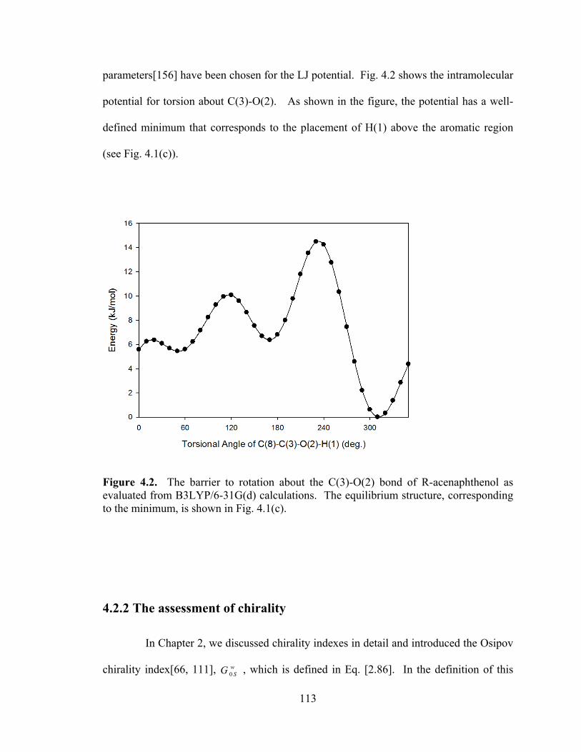
113

parameters[156] have been chosen for the LJ potential. Fig. 4.2 shows the intramolecular

potential for torsion about C(3)-O(2). As shown in the figure, the potential has a well-

defined minimum that corresponds to the placement of H(1) above the aromatic region

(see Fig. 4.1(c)).

Figure 4.2. The barrier to rotation about the C(3)-O(2) bond of R-acenaphthenol as evaluated from B3LYP/6-31G(d) calculations. The equilibrium structure, corresponding to the minimum, is shown in Fig. 4.1(c).

4.2.2 The assessment of chirality

In Chapter 2, we discussed chirality indexes in detail and introduced the Osipov

chirality index[66, 111], wSG 0 , which is defined in Eq. [2.86]. In the definition of this

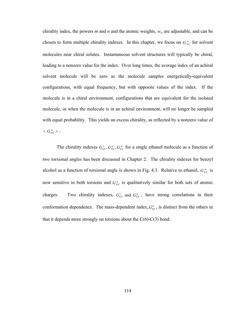
114

chirality index, the powers m and n and the atomic weights, wi, are adjustable, and can be

chosen to form multiple chirality indexes. In this chapter, we focus on wSG 0 for solvent

molecules near chiral solutes. Instantaneous solvent structures will typically be chiral,

leading to a nonzero value for the index. Over long times, the average index of an achiral

solvent molecule will be zero as the molecule samples energetically-equivalent

configurations, with equal frequency, but with opposite values of the index. If the

molecule is in a chiral environment, configurations that are equivalent for the isolated

molecule, or when the molecule is in an achiral environment, will no longer be sampled

with equal probability. This yields an excess chirality, as reflected by a nonzero value of

>< wSG 0 .

The chirality indexes mS

qSS GGG 00

10 ,, for a single ethanol molecule as a function of

two torsional angles has been discussed in Chapter 2. The chirality indexes for benzyl

alcohol as a function of torsional angle is shown in Fig. 4.3. Relative to ethanol, mSG 0 is

now sensitive to both torsions and qSG 0 is qualitatively similar for both sets of atomic

charges. Two chirality indexes, qSS GG 0

10 and , have strong correlations in their

conformation dependence. The mass-dependent index, mSG0 , is distinct from the others in

that it depends more strongly on torsions about the C(6)-C(3) bond.

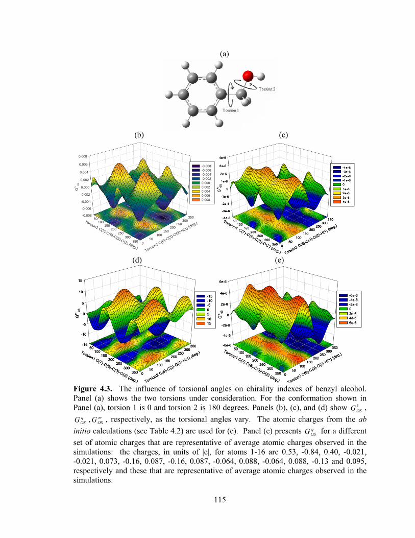
115

(a)

(b) (c)

(d) (e)

Figure 4.3. The influence of torsional angles on chirality indexes of benzyl alcohol. Panel (a) shows the two torsions under consideration. For the conformation shown in Panel (a), torsion 1 is 0 and torsion 2 is 180 degrees. Panels (b), (c), and (d) show 1

OSG , qOSG , m

OSG , respectively, as the torsional angles vary. The atomic charges from the ab initio calculations (see Table 4.2) are used for (c). Panel (e) presents q

OSG for a different set of atomic charges that are representative of average atomic charges observed in the simulations: the charges, in units of |e|, for atoms 1-16 are 0.53, -0.84, 0.40, -0.021, -0.021, 0.073, -0.16, 0.087, -0.16, 0.087, -0.064, 0.088, -0.064, 0.088, -0.13 and 0.095, respectively and these that are representative of average atomic charges observed in the simulations.

-0.008

-0.006

-0.004

-0.002

0.000

0.002

0.004

0.006

0.008

50100

150200

250300

350 050

100150

200250

300350

G1

0S

Torsion1 C(7)-C(6)-C(3)-O(2) (deg.)Torsion2 C(6)-C

(3)-O(2)-H

(1) (deg.)

-0.008 -0.006 -0.004 -0.002 0.000 0.002 0.004 0.006 0.008

116

(a) (b)

(c) (d)

Figure 4.4. The coordinate system used to evaluate chirality indexes for solvent, illustrated for S-PAMD(a). The oxygen lies at the origin of the coordinate system, the carbonyl carbon is on the z-axis, and the amide nitrogen lies in the xz plane. With this coordinate system, the index for an H-bonding solvent is categorized according to two angles (θ and φ) that are used to locate the solvent via its oxygen atom. These angles define a sphere, as shown in (b), which can be used to map out the 3-dimensional variation of the chirality index. The color scale in (b) shows the number of hydrogen-bonded solvents found in the various angle ranges. Panel (c) shows an example of hydrogen-bonding ethanol around S-PAMD. The sphere is centered on the oxygen of S-PAMD with a radius of 3.5Å, which is the maximum O…O distance for H-bonds. The dependence of θ and φ is also important, but is not shown here for simplicity. Panel (d) shows three spheres around the oxygen of S-PAMD. The ethanol is in the second sphere, with an oxygen-oxygen distance between 4 and 7Å.

117

In what regions around the solute will the excess chirality of the solvent be most

significant? To address this question, a solute-based coordinate system is defined as

shown in Fig. 4.4(a). This coordinate system will move with the solute within the

simulation. It is important to realize that the solute is flexible and the atoms defining the

coordinate system undergo intramolecular motion: The coordinate system varies with

time (by a limited amount). For all solutes, the oxygen atom is at the origin of the

coordinate system. For PAMD, as shown in Fig. 4.4(a), C(5) is on the z-axis and N(7) is

in the xz plane. For styrene oxide, C(1) is on the z-axis and C(4) is in the xz-plane while,

for acenaphthenol, C(3) and C(5) define the z-axis and the xz-plane, respectively. With

the coordinate system in place, the angular space is divided into 648 angular bins (see Fig.

4.4(b)) defined by 010=Δθ and 010=Δϕ . This division allows us to associate a excess

chirality with the solvent position about the solute. The resulting average chirality index

is referred to as an “angle-dependent” excess chirality, ϕθ ,0 >< wSG , and integration of this

index over all angles yields >< wSG0 .

Within the simulations, the chirality indexes are evaluated in two ways. First, the

indexes are collected for solvent directly hydrogen-bonded to the chiral solute, as shown

in Fig. 4.4(c). The sphere is centered on the oxygen of S-PAMD with a radius of 3.5Å,

which is the maximum O…O distance for H-bonds. The dependence of θ and φ is also

important, but is not shown here for simplicity. We have found that the chirality transfer

to H-bonded solvent is larger than that for other solvents in the vicinity of the solute. As

a result, we focus primarily on the H-bonded solvent. However, we also examine a

position dependent index rwSG >< 0 for solvent found within a certain distance of the

118

solute oxygen (up to 15 Å), as shown in Fig. 4.4(d). For simulations involving

polarizable fluids, the charge-weighted index, qSG0 , should be more sensitive to the

molecular environment due to the field-dependent fluctuation in atomic charges. As a

result, emphasis is placed on < qSG0 > .

4.2.3. Simulation details

Chirality transfer is evaluated from MD simulations of chiral solute (styrene oxide,

PAMD, or acenaphthenol) surrounded by solvent (ethanol or benzyl alcohol). Each

simulation includes 500 solvent and 4 solute molecules. The solvent density, at 298K, is

0.789g/cm3 for ethanol[162] and 0.990g/cm3 for benzyl alcohol. The latter is slightly

below the experimental density[162] of 1.044 g/cm3 but gave a diffusion coefficient

consistent with experiment[157]. Periodic boundary conditions are applied in the

simulations, with the cutoff chosen as slightly less than half of the box length. Ewald

summations, with conducting boundary conditions,[40] are used for the electrostatic

interactions. In the case of polarizable fluids, the electrostatic forces are first evaluated

according to the Ewald summations, then corrections from the modified electrostatic

potential (Eq. [2.26]) are included. The results reported below correspond to a

momentum space cutoff of 272* ≤k and a position space cut-off of 1592.0=α Å-1 for

benzyl alcohol, and 1891.0=α Å-1 for ethanol.

Independent Nosé-Hoover thermostats are used to generate canonical averages for

translation and rotation. Only the rigid rings in benzyl alcohol and in the three solutes

contribute to the latter. For polarizable models, extended Lagrangian equations of motion

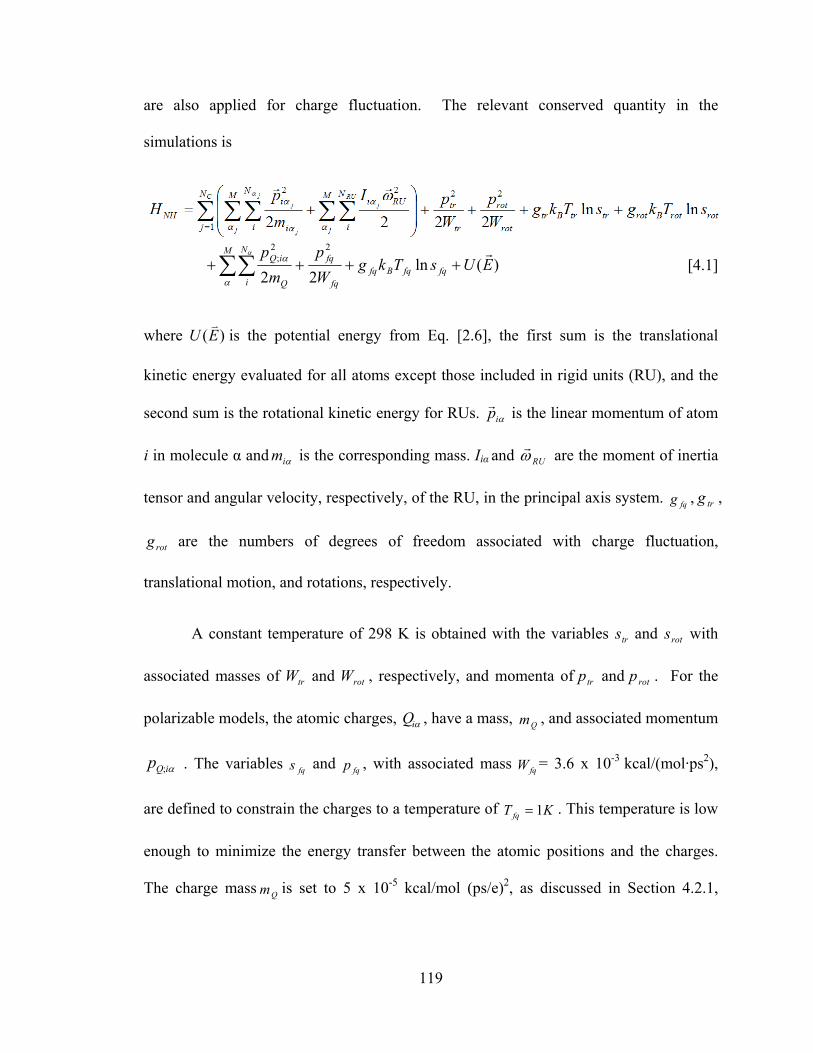
119

are also applied for charge fluctuation. The relevant conserved quantity in the

simulations is

)(ln22

22; EUsTkg

Wp

mp

fqfqBfqfq

fqM N

i Q

iQ r++++∑∑

α

αα

[4.1]

where )(EUv

is the potential energy from Eq. [2.6], the first sum is the translational

kinetic energy evaluated for all atoms except those included in rigid units (RU), and the

second sum is the rotational kinetic energy for RUs. αipr is the linear momentum of atom

i in molecule α and αim is the corresponding mass. Iiα and RUωr are the moment of inertia

tensor and angular velocity, respectively, of the RU, in the principal axis system. fqg , trg ,

rotg are the numbers of degrees of freedom associated with charge fluctuation,

translational motion, and rotations, respectively.

A constant temperature of 298 K is obtained with the variables trs and rots with

associated masses of trW and rotW , respectively, and momenta of trp and rotp . For the

polarizable models, the atomic charges, αiQ , have a mass, Qm , and associated momentum

αiQp ; . The variables fqs and fqp , with associated mass fqW = 3.6 x 10-3 kcal/(mol·ps2),

are defined to constrain the charges to a temperature of KT fq 1= . This temperature is low

enough to minimize the energy transfer between the atomic positions and the charges.

The charge mass Qm is set to 5 x 10-5 kcal/mol (ps/e)2, as discussed in Section 4.2.1,

120

which is small enough to allow a rapid response of the atomic charges to changes in

atomic positions.

The time step for all simulations, except for the fCINTRA solvent, is 0.3 fs. As

discussed elsewhere,[91] a multiple time step algorithm is required for fCINTRA, and the

large and small time steps are 0.1 and 0.01 fs, respectively, for this model. The

equilibration period consists of the first 10 000 steps of each simulation. Following this,

angle-dependent chirality indexes are collected every 20 iterations.

4.2.4 Convergence of the chirality transfer

The evaluation of the excess solvent chirality requires lengthy simulations due to

significant cancellation between instantaneous values of the chirality index. In this

section, the convergence is examined in detail and Fig. 4.5 provides the results of several

tests of convergence.

The first test examines the chirality transfer about an achiral solute. Consider Fig.

4.5(a). The position and angle-dependent excess chiralities are shown in the left and right

panels, respectively. In the right panel, the vertical line at φ=180 corresponds to the

“solute” H(1) positioned in the O(2)-C(3)-C(4) plane and the contours identify the most

probable locations for H-bonded solvent. The two panels show the results of 17 ns

simulations of bulk ethanol, in which four ethanol molecules have been selected and

identified as solutes. The left panel shows the radial dependence of the average chirality

index rqSG >< 0 for solvent molecules with oxygen atoms found at a distance r from the

oxygen atom of a “solute”. As expected, since the “solute” is achiral, the average

121

chirality index is zero at all separations. The right panel shows the angle-dependent

excess chirality, ϕθ ,0 >< qSG , for ethanol H-bonded to the solute. As shown in the panel,

when divided into angular zones, the chirality transfer is small but not zero. This is

exactly analogous to the “chirality” of molecules that are achiral in the isotropic phase

but chiral when deposited on a surface [163]. Thus, each side of the ethanol “solute” is

seen as chiral, but the two sides together cancel out to yield an overall chirality of zero, as

shown in the left panel. The vertical line in the right panel corresponds to the “solute”

H(1) positioned in the O(2)-C(3)-C(4) plane. Thus this line defines the two sides of the

solute, and symmetry about this line is clearly evident in the panel. The overlaid

contours in the right panel identify the most probable angles for finding an H-bonded

solvent. As the probability drops, so does the quality of the average chirality index as

indicated by the loss of symmetry about φ=180o for low probability angles. The legend

shows that ϕθ ,0 >< qSG is less than |10-6| despite the fact that instantaneous values may be

as large as |10-4|. Cancellation is clearly significant and, as a result, lengthy simulations

are required to properly capture the small angle-dependent excess chirality.

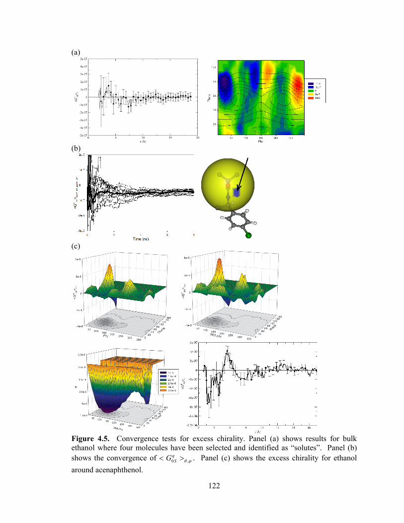
122

(a)

(b)

(c)

Figure 4.5. Convergence tests for excess chirality. Panel (a) shows results for bulk ethanol where four molecules have been selected and identified as “solutes”. Panel (b) shows the convergence of ϕθ ,0 >< q

SG . Panel (c) shows the excess chirality for ethanol around acenaphthenol.

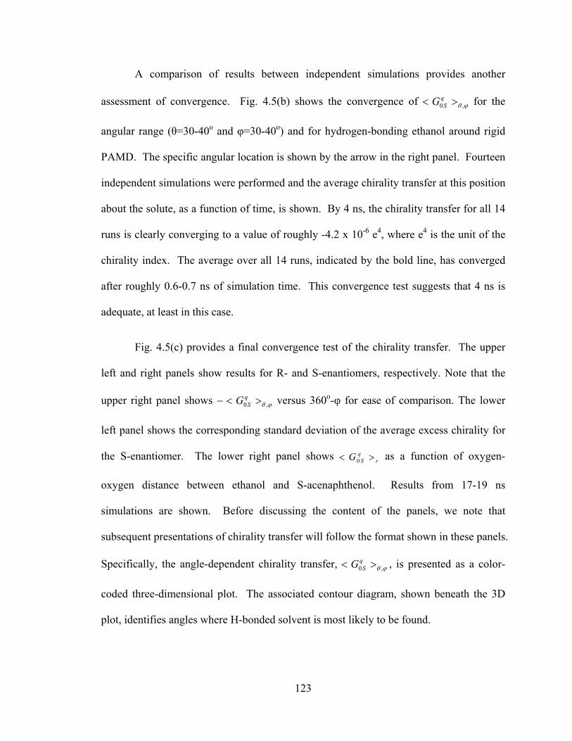
123

A comparison of results between independent simulations provides another

assessment of convergence. Fig. 4.5(b) shows the convergence of ϕθ ,0 >< qSG for the

angular range (θ=30-40o and φ=30-40o) and for hydrogen-bonding ethanol around rigid

PAMD. The specific angular location is shown by the arrow in the right panel. Fourteen

independent simulations were performed and the average chirality transfer at this position

about the solute, as a function of time, is shown. By 4 ns, the chirality transfer for all 14

runs is clearly converging to a value of roughly -4.2 x 10-6 e4, where e4 is the unit of the

chirality index. The average over all 14 runs, indicated by the bold line, has converged

after roughly 0.6-0.7 ns of simulation time. This convergence test suggests that 4 ns is

adequate, at least in this case.

Fig. 4.5(c) provides a final convergence test of the chirality transfer. The upper

left and right panels show results for R- and S-enantiomers, respectively. Note that the

upper right panel shows ϕθ ,0 ><− qSG versus 360o-φ for ease of comparison. The lower

left panel shows the corresponding standard deviation of the average excess chirality for

the S-enantiomer. The lower right panel shows rqSG >< 0 as a function of oxygen-

oxygen distance between ethanol and S-acenaphthenol. Results from 17-19 ns

simulations are shown. Before discussing the content of the panels, we note that

subsequent presentations of chirality transfer will follow the format shown in these panels.

Specifically, the angle-dependent chirality transfer, ϕθ ,0 >< qSG , is presented as a color-

coded three-dimensional plot. The associated contour diagram, shown beneath the 3D

plot, identifies angles where H-bonded solvent is most likely to be found.

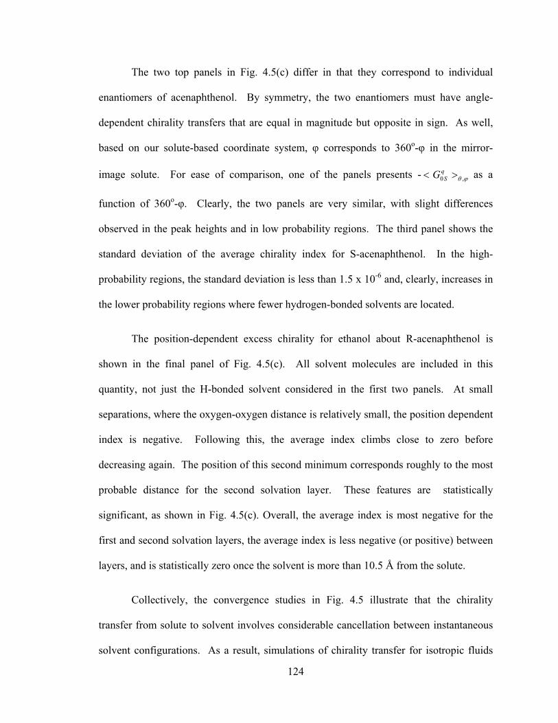
124

The two top panels in Fig. 4.5(c) differ in that they correspond to individual

enantiomers of acenaphthenol. By symmetry, the two enantiomers must have angle-

dependent chirality transfers that are equal in magnitude but opposite in sign. As well,

based on our solute-based coordinate system, φ corresponds to 360o-φ in the mirror-

image solute. For ease of comparison, one of the panels presents - ϕθ ,0 >< qSG as a

function of 360o-φ. Clearly, the two panels are very similar, with slight differences

observed in the peak heights and in low probability regions. The third panel shows the

standard deviation of the average chirality index for S-acenaphthenol. In the high-

probability regions, the standard deviation is less than 1.5 x 10-6 and, clearly, increases in

the lower probability regions where fewer hydrogen-bonded solvents are located.

The position-dependent excess chirality for ethanol about R-acenaphthenol is

shown in the final panel of Fig. 4.5(c). All solvent molecules are included in this

quantity, not just the H-bonded solvent considered in the first two panels. At small

separations, where the oxygen-oxygen distance is relatively small, the position dependent

index is negative. Following this, the average index climbs close to zero before

decreasing again. The position of this second minimum corresponds roughly to the most

probable distance for the second solvation layer. These features are statistically

significant, as shown in Fig. 4.5(c). Overall, the average index is most negative for the

first and second solvation layers, the average index is less negative (or positive) between

layers, and is statistically zero once the solvent is more than 10.5 Å from the solute.

Collectively, the convergence studies in Fig. 4.5 illustrate that the chirality

transfer from solute to solvent involves considerable cancellation between instantaneous

solvent configurations. As a result, simulations of chirality transfer for isotropic fluids

125

should monitor the fluid properties for a minimum of several nanoseconds. With these

considerations in mind, the simulations of chirality transfer in benzyl alcohol and in

ethanol are conducted for a minimum of 10 ns and 17 ns, respectively. The chirality

transfers reported in Section 4.3 have been averaged over the four solutes in the

simulation cell, for a total monitoring time of 40-68 ns. The only exception is the

fCINTRA ethanol model where we have found that the chirality transfer converges more

quickly and, since the fCINTRA simulations are demanding, we report results for 4 ns.

4.3. Results and discussion

4.3.1 Analyte solvation

Before assessing the chirality transfer, we begin by examining the intermolecular

structure, and the hydrogen-bonding, in the bulk solvents and in solvents in the vicinity of

solute. Fig. 4.6 shows the radial distribution between oxygens for the bulk solvent and

for solvent about the solute. A comparison of hydrogen bonding events in the bulk and

near the chiral solutes is presented in Table 4.3. The structural definition of hydrogen

bonding[120] has been discussed in Section 3.3.2.

Consider first the hydrogen bonding in ethanol. Styrene oxide disrupts the

solvent H-bonding network only weakly, with a few percent fewer ethanol molecules

participating in two hydrogen bonds and a small increase in the number that have only

one hydrogen bond. The hydrogen-bonding structure of ethanol is disrupted much more

significantly around acenaphthenol and PAMD, with a decrease of 13-18% in the number

of solvent with two H-bonds and a commensurate increase of 13-18% in the number of

solvent in the vicinity of the solute with only one hydrogen bond. A similar situation

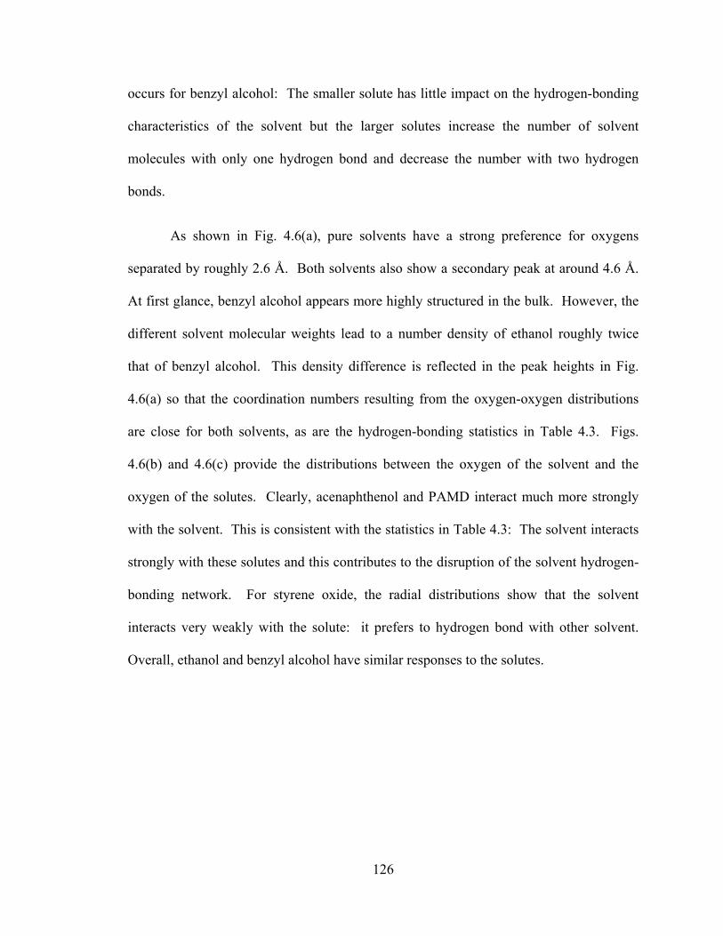
126

occurs for benzyl alcohol: The smaller solute has little impact on the hydrogen-bonding

characteristics of the solvent but the larger solutes increase the number of solvent

molecules with only one hydrogen bond and decrease the number with two hydrogen

bonds.

As shown in Fig. 4.6(a), pure solvents have a strong preference for oxygens

separated by roughly 2.6 Å. Both solvents also show a secondary peak at around 4.6 Å.

At first glance, benzyl alcohol appears more highly structured in the bulk. However, the

different solvent molecular weights lead to a number density of ethanol roughly twice

that of benzyl alcohol. This density difference is reflected in the peak heights in Fig.

4.6(a) so that the coordination numbers resulting from the oxygen-oxygen distributions

are close for both solvents, as are the hydrogen-bonding statistics in Table 4.3. Figs.

4.6(b) and 4.6(c) provide the distributions between the oxygen of the solvent and the

oxygen of the solutes. Clearly, acenaphthenol and PAMD interact much more strongly

with the solvent. This is consistent with the statistics in Table 4.3: The solvent interacts

strongly with these solutes and this contributes to the disruption of the solvent hydrogen-

bonding network. For styrene oxide, the radial distributions show that the solvent

interacts very weakly with the solute: it prefers to hydrogen bond with other solvent.

Overall, ethanol and benzyl alcohol have similar responses to the solutes.

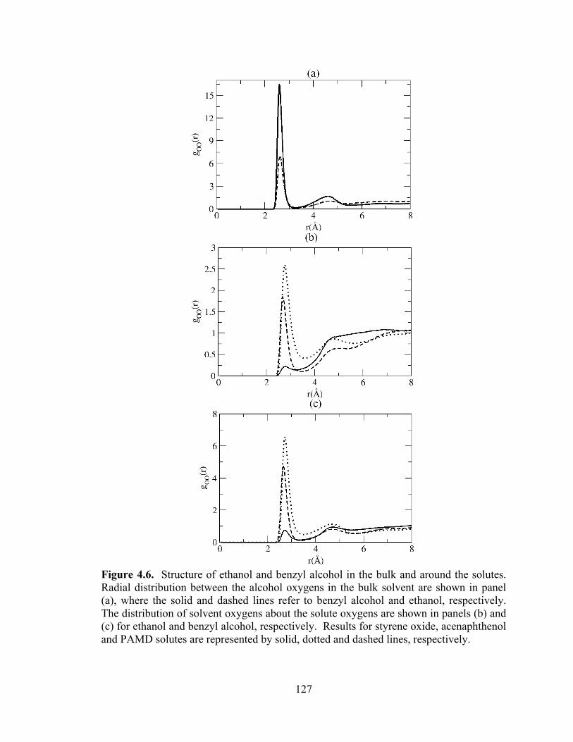
127

Figure 4.6. Structure of ethanol and benzyl alcohol in the bulk and around the solutes. Radial distribution between the alcohol oxygens in the bulk solvent are shown in panel (a), where the solid and dashed lines refer to benzyl alcohol and ethanol, respectively. The distribution of solvent oxygens about the solute oxygens are shown in panels (b) and (c) for ethanol and benzyl alcohol, respectively. Results for styrene oxide, acenaphthenol and PAMD solutes are represented by solid, dotted and dashed lines, respectively.

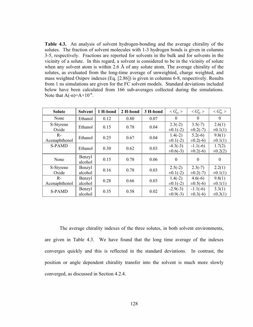
128

Table 4.3. An analysis of solvent hydrogen-bonding and the average chirality of the solutes. The fraction of solvent molecules with 1-3 hydrogen bonds is given in columns 3-5, respectively. Fractions are reported for solvents in the bulk and for solvents in the vicinity of a solute. In this regard, a solvent is considered to be in the vicinity of solute when any solvent atom is within 2.6 Å of any solute atom. The average chirality of the solutes, as evaluated from the long-time average of unweighted, charge weighted, and mass weighted Osipov indexes (Eq. [2.86]) is given in columns 6-8, respectively. Results from 1 ns simulations are given for the FC solvent models. Standard deviations included below have been calculated from 166 sub-averages collected during the simulations. Note that A(-n)=A×10-n.

Solute Solvent 1 H-bond 2 H-bond 3 H-bond >< 1

0SG >< qSG0 >< m

SG0

None Ethanol 0.12 0.80 0.07 0 0 0S-Styrene

Oxide Ethanol 0.15 0.78 0.04 2.3(-2) ±0.1(-2)

3.5(-7)±0.2(-7)

2.6(1)±0.1(1)

R-Acenaphthenol Ethanol 0.25 0.67 0.04 1.4(-2)

±0.1(-2) 5.2(-6)

±0.2(-6)9.8(1)

±0.1(1)S-PAMD Ethanol 0.30 0.62 0.03 -4.3(-3)

±0.6(-3) -1.1(-6)±0.2(-6)

1.7(2)±0.2(2)

None Benzyl alcohol 0.15 0.78 0.06 0 0 0

S-Styrene Oxide

Benzyl alcohol 0.16 0.78 0.03 2.5(-2)

±0.1(-2) 2.3(-7)

±0.2(-7)2.2(1)

±0.1(1)R-

Acenaphthenol Benzyl alcohol 0.28 0.66 0.03 1.4(-2)

±0.1(-2) 4.6(-6)

±0.5(-6)9.8(1)

±0.1(1)

S-PAMD Benzyl alcohol 0.35 0.58 0.02 -2.9(-3)

±0.9(-3) -1.1(-6)±0.3(-6)

3.3(1)±0.3(1)

The average chirality indexes of the three solutes, in both solvent environments,

are given in Table 4.3. We have found that the long time average of the indexes

converges quickly and this is reflected in the standard deviations. In contrast, the

position or angle dependent chirality transfer into the solvent is much more slowly

converged, as discussed in Section 4.2.4.

129

4.3.2 The solvent representation: Is polarizability important?

Typical simulations employ nonpolarizable molecular models so that

instantaneous changes in the molecular force field, as represented by the potential

parameters, are not allowed. However, the chirality transfer from solute to solvent may

involve solvent polarization, since the solvent experiences and responds to the chiral field

of the solute. In this section, we examine the excess chirality of ethanol about PAMD as

predicted by three solvent models. First, a nonpolarizable solvent model is considered.

Second, we examine a partially-polarizable model (the FC model) which shares all the

same potential parameters as the nonpolarizable model, except that the atomic charges

vary instantaneously. Finally, ethanol is represented by a fully-polarizable model (the

fCINTRA model) that is identical to the FC model except that some intramolecular

potential parameters fluctuate instantaneously and the fCINTRA-optimized LJ

parameters for O(2) and H(1) have been selected. The similarity between these three

models provides a clear basis for an assessment of the relationship between solvent

polarizability and chirality transfer.

The angle-dependent excess chirality, ϕθ ,0 >< qSG , is shown in Fig. 4.7 as a

function of solvent position about PAMD. The three panels in Fig. 4.7 differ in that

ethanol is represented by the nonpolarizable model, the FC model, and the fCINTRA

model. The contour plots in Fig. 4.7 identify the high probability regions for hydrogen-

bonded ethanol around PAMD. All three solvent representations give very similar

probability distributions: Polarizability has a small impact on the distribution of ethanol

around PAMD. In Figs. 4.7(d)-4.7(e), two snapshots of ethanol and PAMD,

corresponding to the high probability region around θ=0-10 degrees, are shown. The

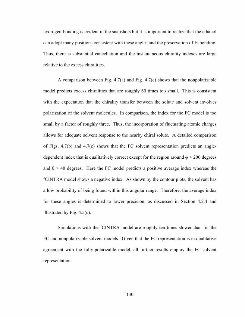
130

hydrogen-bonding is evident in the snapshots but it is important to realize that the ethanol

can adopt many positions consistent with these angles and the preservation of H-bonding.

Thus, there is substantial cancellation and the instantaneous chirality indexes are large

relative to the excess chiralities.

A comparison between Fig. 4.7(a) and Fig. 4.7(c) shows that the nonpolarizable

model predicts excess chiralities that are roughly 60 times too small. This is consistent

with the expectation that the chirality transfer between the solute and solvent involves

polarization of the solvent molecules. In comparison, the index for the FC model is too

small by a factor of roughly three. Thus, the incorporation of fluctuating atomic charges

allows for adequate solvent response to the nearby chiral solute. A detailed comparison

of Figs. 4.7(b) and 4.7(c) shows that the FC solvent representation predicts an angle-

dependent index that is qualitatively correct except for the region around φ > 200 degrees

and θ > 40 degrees. Here the FC model predicts a positive average index whereas the

fCINTRA model shows a negative index. As shown by the contour plots, the solvent has

a low probability of being found within this angular range. Therefore, the average index

for these angles is determined to lower precision, as discussed in Section 4.2.4 and

illustrated by Fig. 4.5(c).

Simulations with the fCINTRA model are roughly ten times slower than for the

FC and nonpolarizable solvent models. Given that the FC representation is in qualitative

agreement with the fully-polarizable model, all further results employ the FC solvent

representation.

131

(a) (d)

(b) (e)

(c)

Figure 4.7. The impact of solvent polarizability on chirality transfer: The angle-dependence of ϕθ ,0 >< q

SG for ethanol hydrogen-bonded to the oxygen of S-PAMD. Results from MD simulations are shown for a non-polarizable model (a), a fluctuating charge (FC) representation (b) and the fully-polarizable fCINTRA ethanol model (c). Panels (d) and (e) show hydrogen-bonding ethanol in the high probability regions.

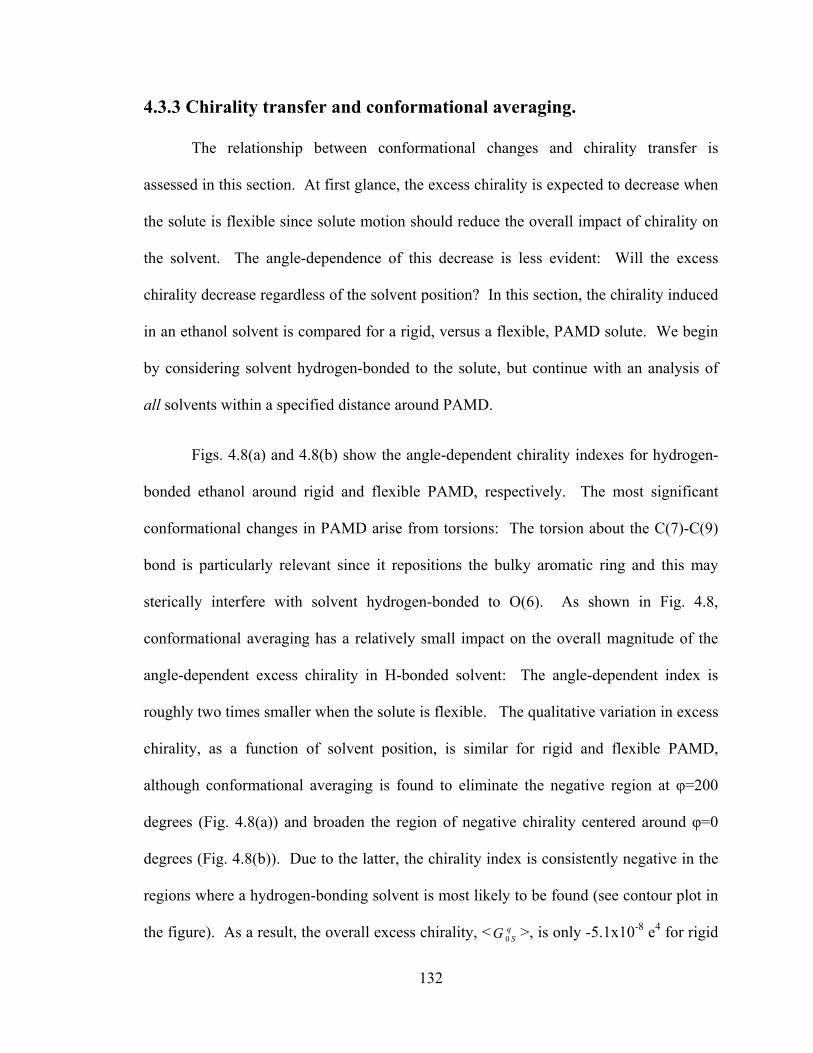
132

4.3.3 Chirality transfer and conformational averaging.

The relationship between conformational changes and chirality transfer is

assessed in this section. At first glance, the excess chirality is expected to decrease when

the solute is flexible since solute motion should reduce the overall impact of chirality on

the solvent. The angle-dependence of this decrease is less evident: Will the excess

chirality decrease regardless of the solvent position? In this section, the chirality induced

in an ethanol solvent is compared for a rigid, versus a flexible, PAMD solute. We begin

by considering solvent hydrogen-bonded to the solute, but continue with an analysis of

all solvents within a specified distance around PAMD.

Figs. 4.8(a) and 4.8(b) show the angle-dependent chirality indexes for hydrogen-

bonded ethanol around rigid and flexible PAMD, respectively. The most significant

conformational changes in PAMD arise from torsions: The torsion about the C(7)-C(9)

bond is particularly relevant since it repositions the bulky aromatic ring and this may

sterically interfere with solvent hydrogen-bonded to O(6). As shown in Fig. 4.8,

conformational averaging has a relatively small impact on the overall magnitude of the

angle-dependent excess chirality in H-bonded solvent: The angle-dependent index is

roughly two times smaller when the solute is flexible. The qualitative variation in excess

chirality, as a function of solvent position, is similar for rigid and flexible PAMD,

although conformational averaging is found to eliminate the negative region at φ=200

degrees (Fig. 4.8(a)) and broaden the region of negative chirality centered around φ=0

degrees (Fig. 4.8(b)). Due to the latter, the chirality index is consistently negative in the

regions where a hydrogen-bonding solvent is most likely to be found (see contour plot in

the figure). As a result, the overall excess chirality, < qSG 0 >, is only -5.1x10-8 e4 for rigid

133

PAMD but is -2.6x10-7 e4 when the solute is flexible. Thus, the angle-dependent excess

chirality decreases as a result of solute flexibility but the overall, angle-averaged value

increases due to qualitative changes in the H-bonded solvent, particularly when the

solvent is positioned around φ=0 degrees. From the PAMD-based coordinate system

shown in Fig. 4.4(a), this angular range corresponds to solvent near the N(7)-C(5)-O(6)

plane (see Fig. 4.1). From Fig. 2.9, these results are consistent with the H-bonded solvent

near this plane favoring angles greater than 180o for torsion 2 when the solute is flexible.

(a) (b)

(c) (d)

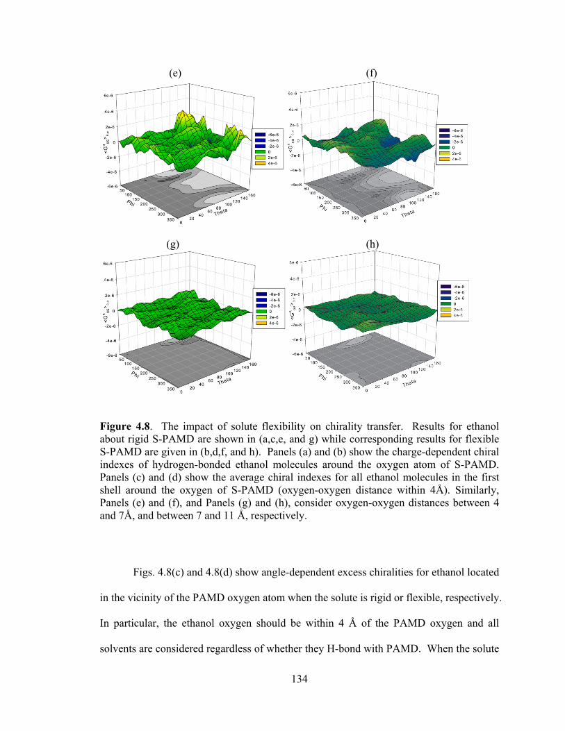
134

(e) (f)

(g) (h)

Figure 4.8. The impact of solute flexibility on chirality transfer. Results for ethanol about rigid S-PAMD are shown in (a,c,e, and g) while corresponding results for flexible S-PAMD are given in (b,d,f, and h). Panels (a) and (b) show the charge-dependent chiral indexes of hydrogen-bonded ethanol molecules around the oxygen atom of S-PAMD. Panels (c) and (d) show the average chiral indexes for all ethanol molecules in the first shell around the oxygen of S-PAMD (oxygen-oxygen distance within 4Å). Similarly, Panels (e) and (f), and Panels (g) and (h), consider oxygen-oxygen distances between 4 and 7Å, and between 7 and 11 Å, respectively.

Figs. 4.8(c) and 4.8(d) show angle-dependent excess chiralities for ethanol located

in the vicinity of the PAMD oxygen atom when the solute is rigid or flexible, respectively.

In particular, the ethanol oxygen should be within 4 Å of the PAMD oxygen and all

solvents are considered regardless of whether they H-bond with PAMD. When the solute

135

is rigid, certain areas about the oxygen are simply inaccessible to the solvent and this is

evident in the contour plot of Fig. 4.8(c). Figs. 4.8(c) and 4.8(d) are fairly distinct: The

flexibility of the solute has an impact on the spatial characteristics of the chirality transfer

when all solvents are considered.

A comparison of Figs. 4.8(b) and 4.8(d) reveals distinctions between H-bonded

ethanol and ethanol in the vicinity of the solute oxygen. Specifically, as shown by the

contour plots in Figs. 4.8(b) and 4.8(d), hydrogen-bonded ethanol molecules have a

restricted orientation relative to the solute and form a subset of the ethanol molecules

found near the PAMD oxygen. Thus, Fig. 4.8(d) includes a larger number of ethanol

molecules, and these display a broad range of orientations relative to the PAMD. As a

result, the excess chirality in Fig. 4.8(d) varies less with the solvent position, although it

is important to note that the angle-dependent excess chirality is still negative, although

smaller in magnitude, in the primary hydrogen bonding regions. The angle-averaged

excess chirality for H-bonded ethanol (Table 4.5) is -2.6x10-7 e4 whereas the equivalent

average (Table 4.4), for all ethanol molecules in the vicinity of the PAMD oxygen, is

-2.2x10-7 e4. The extensive cancellation of instantaneous indexes, to yield the excess

chirality, is evident from a comparison with the conformational variations in qSG 0 shown

in Fig. 2.9 , where values as high as ±8x10-5 e4 were obtained.

For solvent “far” from the chiral solute, the local environment is achiral, on

average, and the angle-dependent excess chirality should vanish for all angles. Figs.

4.8(e)-(h) show the decrease in the angle-dependent excess chirality as the solvent is

farther from the solute. Solvents within 7-11 Å of the PAMD oxygen atom are found to

have an angle-dependent chirality index that is roughly ten times smaller than for

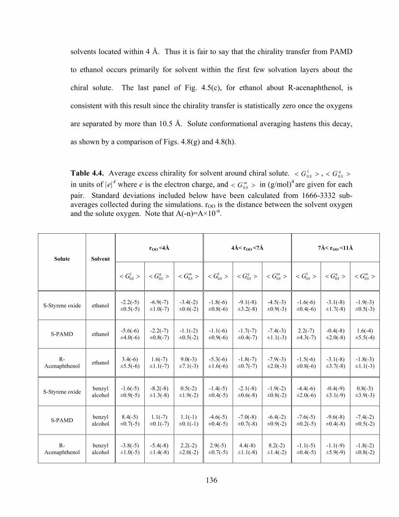
136

solvents located within 4 Å. Thus it is fair to say that the chirality transfer from PAMD

to ethanol occurs primarily for solvent within the first few solvation layers about the

chiral solute. The last panel of Fig. 4.5(c), for ethanol about R-acenaphthenol, is

consistent with this result since the chirality transfer is statistically zero once the oxygens

are separated by more than 10.5 Å. Solute conformational averaging hastens this decay,

as shown by a comparison of Figs. 4.8(g) and 4.8(h).

Table 4.4. Average excess chirality for solvent around chiral solute. >< 1

0 SG , >< qSG 0

in units of |e|4 where e is the electron charge, and >< mSG 0 in (g/mol)4 are given for each

pair. Standard deviations included below have been calculated from 1666-3332 sub-averages collected during the simulations. rOO is the distance between the solvent oxygen and the solute oxygen. Note that A(-n)=A×10-n.

Solute Solvent

rOO <4Å 4Å< rOO <7Å 7Å< rOO <11Å

>< 10SG >< q

SG0 >< mSG0 >< 1

0SG >< qSG0 >< m

SG0 >< 10SG >< q

SG0 >< mSG0

S-Styrene oxide ethanol -2.2(-5) ±0.5(-5)

-6.9(-7) ±1.0(-7)

-3.4(-2) ±0.6(-2)

-1.8(-6) ±0.8(-6)

-9.1(-8) ±3.2(-8)

-4.5(-3) ±0.9(-3)

-1.6(-6) ±0.4(-6)

-3.1(-8) ±1.7(-8)

-1.9(-3) ±0.5(-3)

S-PAMD ethanol -5.6(-6) ±4.0(-6)

-2.2(-7) ±0.8(-7)

-1.1(-2) ±0.5(-2)

-1.1(-6) ±0.9(-6)

-1.7(-7) ±0.4(-7)

-7.4(-3) ±1.1(-3)

2.2(-7) ±4.3(-7)

-0.4(-8) ±2.0(-8)

1.6(-4) ±5.5(-4)

R-Acenaphthenol ethanol 3.4(-6)

±5.5(-6) 1.6(-7)

±1.1(-7) 9.0(-3)

±7.1(-3) -5.3(-6) ±1.6(-6)

-1.8(-7) ±0.7(-7)

-7.9(-3) ±2.0(-3)

-1.5(-6) ±0.8(-6)

-3.1(-8) ±3.7(-8)

-1.8(-3) ±1.1(-3)

S-Styrene oxide benzyl alcohol

-1.6(-5) ±0.9(-5)

-8.2(-8) ±1.3(-8)

0.5(-2) ±1.9(-2)

-1.4(-5) ±0.4(-5)

-2.1(-8) ±0.6(-8)

-1.9(-2) ±0.8(-2)

-4.4(-6) ±2.0(-6)

-0.4(-9) ±3.1(-9)

0.8(-3) ±3.9(-3)

S-PAMD benzyl alcohol

8.4(-5) ±0.7(-5)

1.1(-7) ±0.1(-7)

1.1(-1) ±0.1(-1)

-4.6(-5) ±0.4(-5)

-7.0(-8) ±0.7(-8)

-6.4(-2) ±0.9(-2)

-7.6(-5) ±0.2(-5)

-9.6(-8) ±0.4(-8)

-7.4(-2) ±0.5(-2)

R-Acenaphthenol

benzyl alcohol

-3.8(-5) ±1.0(-5)

-5.4(-8) ±1.4(-8)

2.2(-2) ±2.0(-2)

2.9(-5) ±0.7(-5)

4.4(-8) ±1.1(-8)

8.2(-2) ±1.4(-2)

-1.1(-5) ±0.4(-5)

-1.1(-9) ±5.9(-9)

-1.8(-2) ±0.8(-2)

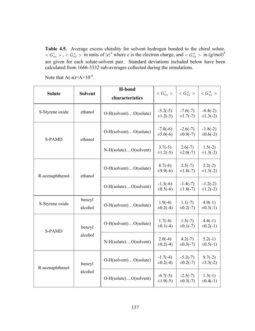
137

Table 4.5. Average excess chirality for solvent hydrogen bonded to the chiral solute. >< 1

0 SG , >< qSG 0 in units of |e|4 where e is the electron charge, and >< m

SG 0 in (g/mol)4

are given for each solute-solvent pair. Standard deviations included below have been calculated from 1666-3332 sub-averages collected during the simulations.

Note that A(-n)=A×10-n.

Solute Solvent H-bond

characteristics >< 1

0 SG >< qSG 0 >< m

SG 0

S-Styrene oxide ethanol O-H(solvent)…O(solute) -3.2(-5) ±1.2(-5)

-7.6(-7) ±1.7(-7)

-6.4(-2) ±1.3(-2)

S-PAMD ethanol O-H(solvent)…O(solute) -7.0(-6)

±5.0(-6) -2.6(-7) ±0.9(-7)

-1.8(-2) ±0.6(-2)

N-H(solute)…O(solvent) 3.7(-5) ±1.2(-5)

2.6(-7) ±2.0(-7)

1.5(-2) ±1.3(-2)

R-acenaphthenol ethanol O-H(solvent)…O(solute) 8.7(-6)

±9.9(-6) 2.5(-7)

±1.8(-7) 2.2(-2)

±1.3(-2)

O-H(solute)…O(solvent) -1.3(-6) ±8.5(-6)

-1.4(-7) ±1.8(-7)

-1.2(-2) ±1.2(-2)

S-Styrene oxide benzyl

alcohol O-H(solvent)…O(solute) 1.9(-4) ±0.2(-4)

1.1(-7) ±0.2(-7)

4.9(-1) ±0.3(-1)

S-PAMD benzyl

alcohol

O-H(solvent)…O(solute) 1.7(-4) ±0.1(-4)

1.5(-7) ±0.1(-7)

4.4(-1) ±0.2(-1)

N-H(solute)…O(solvent) 2.0(-4) ±0.2(-4)

4.2(-7) ±0.3(-7)

5.2(-1) ±0.5(-1)

R-acenaphthenol benzyl

alcohol

O-H(solvent)…O(solute) -1.7(-4) ±0.2(-4)

-5.2(-7) ±0.2(-7)

9.7(-2) ±3.3(-2)

O-H(solute)…O(solvent) -6.7(-5) ±1.9(-5)

-2.5(-7) ±0.3(-7)

1.3(-1) ±0.4(-1)

138

Overall excess chiralities are presented in Table 4.4. The averages have been

evaluated over three spatial regions: roo ≤ 4Å, 4Å < roo ≤ 7Å, and 7Å < roo ≤ 11Å. By

comparison with the radial distributions in Fig. 4.6, this first region includes the contact

peak, the second region includes the second solvation shell and some of the third, while

the last region incorporates solvents “far” from the solute. As shown in the table, the

chirality transfer systematically decreases from the contact region to the second solvation

shell to the outer region. In general, the sign of the chirality transfer may remain

unchanged or alternate between regions. However, as illustrated by Fig. 4.5(c), the

position-dependent excess chirality may switch signs within these ranges so that the

averages in Table 4.4 may include some cancellation.

4.3.4 Contact points and chirality transfer.

In chiral chromatography, the number of interaction points between the analyte

and the chiral selector is essential to the recognition process. In this section, we explore

the relationship between the number of solute-solvent interactions, and the chirality

transferred to nearby solvent molecules.

Fig. 4.9 provides the angle-dependent chirality index for ethanol about the three

solutes. The location of hydrogen-bonded solvent, relative to the solute oxygen, is

different for all three solutes, as indicated by the contour plots. The angle-dependent

chirality indexes are distinct as well. Panels 4.9(d)-4.9(f) indicate the long-time average

values for the unweighted, charge-weighted, and mass-weighted indexes at angles

corresponding to the most probable location for H-bonded solvent. A representative

139

snapshot is provided to show an H-bonded solvent molecule in the most probable

location and having an instantaneous index of the same sign as the time averaged values.

The angle-dependent chirality index for ethanol about acenaphthenol (Fig. 4.9(b))

has several well-defined regions, but these mostly lie outside the most probable locations

for the solvent. Overall, the average index (see Table 4.5) is small. Focusing on the most

probable solvent location, the long-time average of each index is negative. From Fig. 2.9,

this corresponds to torsion 2 having an average angle greater than 180 degrees. A

representative snapshot is provided in Fig. 4.9(e). When ethanol hydrogen-bonds to

styrene oxide(Fig. 4.9(a)), the chirality transferred to the solvent is strongly dependent on

the position of the solvent. However, the overall excess chirality in Table 4.5 is an order

of magnitude smaller than angle-dependent values due to cancellation. From Fig. 4.9(a),

the long-time average of each index, for solvent in the most probable location is positive.

This corresponds to an average angle for torsion 2 that is less than 180 degrees, as shown

in the snapshot in Fig. 4.9(d). Thus, styrene oxide and acenaphthenol have different

impacts on the conformations of H-bonded solvent. For ethanol about PAMD, the angle-

dependent chirality induced in the solvent is smaller than for the other two solutes (note

that the vertical scales are the same in Figs. 4.9(a), (b), and (c)). However the index is

consistently negative in regions where the H-bonded solvent is most likely located, and

the overall average index, >< qSG0 , in Table 4.5 is comparable with the other solutes.

Fig. 4.10 gives the overall chirality index for benzyl alcohol about the three

solutes. As with ethanol, the angle-dependent excess chirality is qualitatively different

for all three solutes. The angle-dependence is largest for acenaphthenol where the index

is negative over a significant angular range that includes the most probable angles for H-

140

bonding solvents. Acenaphthenol has an extended aromatic region, relative to the other

two solutes, and it is not surprising that chirality transfer is larger for this solute. Fig.

4.10(e) shows an H-bonded benzyl alcohol positioned at angles consistent with the most

probable location for H-bonded solvent about acenaphthenol. The long-time average

values for the three indexes, at this location, indicate that the solvent prefers to have

torsion 2 between 270-300 degrees and torsion 1 between 140-170 degrees (or

equivalently, between 320-350 degrees).

Although it is tempting to directly compare results for ethanol and benzyl alcohol,

this is problematic since the chirality index has some residual dependence on the number

of atoms in the solvent. As well, the relationship between the index and the molecular

structure is complex, although the similarity between Figs. 2.9 and 4.3 implies that some

cautionary remarks can be made. With this in mind, we note that Figs. 4.9 and 4.10

suggest that acenaphthenol has the most pronounced impact on the solvent since the

angle-dependence in the chirality index is largest for this solute. The stronger impact of

acenaphthenol suggests that, for this solute, localized hydrogen-bonded solvent has a

stronger preference for certain chiral configurations. This may be related to the overall

accessibility of the hydrogen-bonding group following the molecular shape and the

restricted conformations available for this solute.

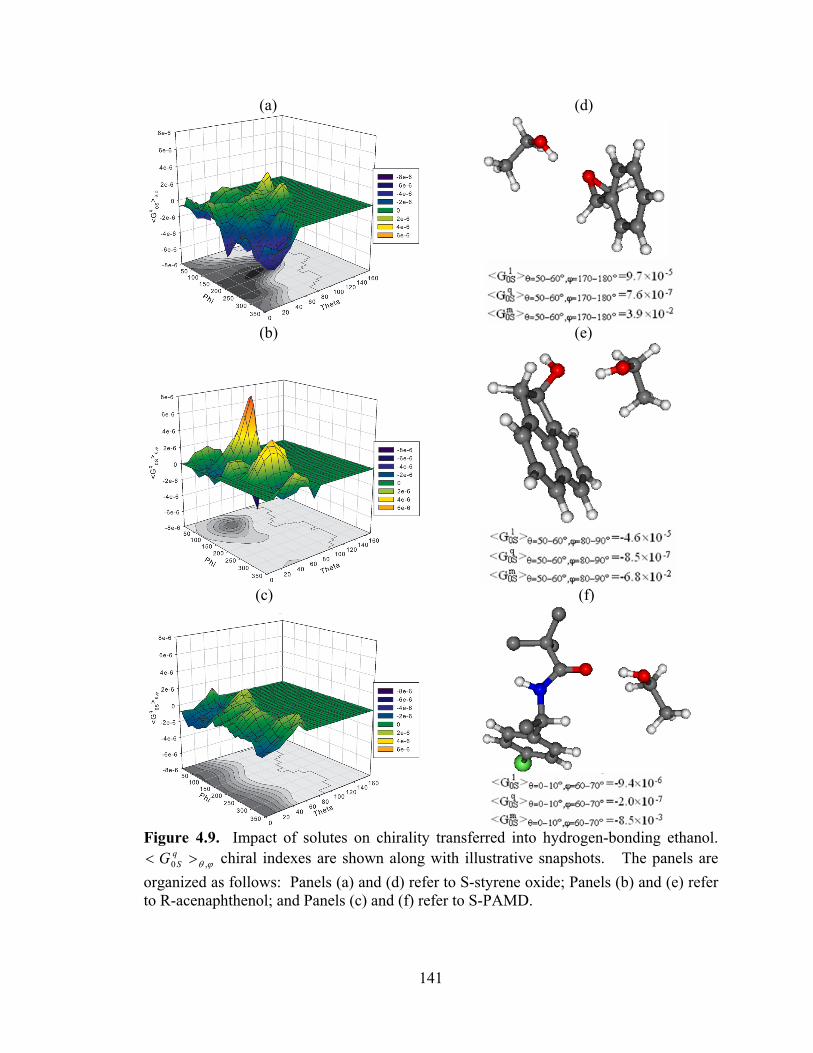
141

(a) (d)

(b) (e)

(c) (f)

Figure 4.9. Impact of solutes on chirality transferred into hydrogen-bonding ethanol.

ϕθ ,0 >< qSG chiral indexes are shown along with illustrative snapshots. The panels are

organized as follows: Panels (a) and (d) refer to S-styrene oxide; Panels (b) and (e) refer to R-acenaphthenol; and Panels (c) and (f) refer to S-PAMD.

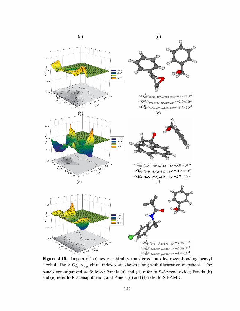
142

(a) (d)

(b) (e)

(c) (f)

Figure 4.10. Impact of solutes on chirality transferred into hydrogen-bonding benzyl alcohol. The ϕθ ,0 >< q

SG chiral indexes are shown along with illustrative snapshots. The panels are organized as follows: Panels (a) and (d) refer to S-Styrene oxide; Panels (b) and (e) refer to R-acenaphthenol; and Panels (c) and (f) refer to S-PAMD.

143

Table 4.5 gives the angle-averaged chirality index for hydrogen-bonded solvent.

For ethanol and benzyl alcohol, the average charge-dependent index < qSG0 > is less than

10-6 for all solutes. In light of the conformational dependence of this index, shown in

Figs. 2.9 and 4.3, these averages clearly reflect significant cancellation so that, overall,

the amount of chirality transferred is small. Despite the small overall average, a stronger

spatial dependence is present and this is evident in the angular distribution of the average

index shown in Figs. 4.9 and 4.10. Thus, within certain spatial regions about the solute,

the chirality transfer may be significant and much larger than the angle-averaged value.

In bulk benzyl alcohol, inter-solvent π-π interactions are possible. This situation

differs from chromatographic separations where the solvent does not include aromatic

rings but the analytes usually do. To explore this fundamental difference, we have also

examined the solvation of acenaphthenol in a mixed solvent. Specifically, simulations of

a binary n-hexane/benzyl alcohol solvent around acenaphthenol were performed. Here,

the n-hexane is nonpolarizable and is the major solvent component. Interestingly, we

found that the angle-dependent chirality transfer to benzyl alcohol was qualitatively very

similar to Fig. 4.10(c), but smaller in magnitude. The similarity in the 3D surfaces likely

reflects the overall structural constraints placed on an H-bonding solvent molecule. On

the other hand, the decrease in magnitude for the mixed solvent suggests that benzyl

alcohol samples more conformations in this environment. This follows from the fact that

an H-bonded benzyl alcohol will be mostly surrounded by n-hexane in the mixed solvent.

In the absence of n-hexane, the benzyl alcohol molecule H-bonded to the solute will be

surrounded by other alcohols, and these H-bond extensively forming a more structured

local environment.

144

4.4. Conclusions

In this chapter, the chirality transfer from a chiral solute to an achiral solvent has

been assessed. The importance of solvent polarizability, conformational averaging, and

the details of the solvent-solute interactions have been considered. We have found that

chirality transfer is most evident for solvent molecules directly H-bonded to the solute.

In addition, ethanol and benzyl alcohol both show a clear relationship between excess

chirality and position of the solvent relative to the chiral solute. That is, chirality transfer

is larger at certain positions about the solute.

Ethanol provided the basis for examining the relationship between solvent

polarization and chirality transfer. Here, solvation of PAMD was examined for a

nonpolarizable ethanol, a fluctuating charge representation of ethanol, and a fully

polarizable ethanol model where the atomic charges and the intramolecular potential vary

with the molecular environment. Inclusion of solvent polarization was found to be very

important, as the solvent must respond to the chiral field of the solute.

The impact of conformational averaging was explored for PAMD. Here the

chirality transfer was assessed for ethanol about a rigid and a flexible PAMD solute. As

expected, conformation averaging decreases the magnitude of the angle-dependent

chirality transfer, by a factor of roughly two, but it also changes some of the

characteristics of the angular dependence of the chirality transfer: In certain regions, the

solvent molecules adopt different conformations depending on the flexibility of PAMD.

The impact of this is significant for PAMD: Solute rigidity has increased the overall

chirality transfer via a reduction in cancellation. Considering PAMD, the chirality

145

transfer was also assessed as the solvent was farther away from the chiral solute. We

have found that the chirality transfer decreases quickly and a 3D representation is

essentially featureless for solvent within 7-11 Å from the chiral solute.

The Osipov chirality index[66] formed the basis of the analysis of chirality

transfer. Long-time averages of this index, for solvents located at various positions about

the solute, identify the excess chirality present in the solvent molecules due to the

presence of a chiral solute. Three indexes were examined: One determined by structure

alone, another weighed by atomic mass, and a third dependent on atomic charges. The

Osipov index is directly related to molecular shape, and can be adapted to emphasize

charge fluctuations, proximate atoms, larger atoms, etc. The spatial decomposition of

multiple time-averaged indexes can be used to generate an average structure of the

solvent about the solute, as a function of the solvent position. This, in turn, may prove

useful in predicting the solvent contributions to experimental properties, such as VCD

spectra, without the requirement for individual snapshot analysis.

146

Chapter 5 Chirality transfer from chiral surfaces to nearby solvents In this chapter, chirality transfer from chiral surfaces to achiral solvents is

discussed. The study is based on MD simulations of four solvents (ethanol, 2-propanol,

ethanol/n-hexane, and 2-propanol/n-hexane) and three brush-type selective interfaces

(Whelk-O1, DNB-phenylglycine, and DNB-leucine). Emphasis is placed on the location

of the chirality transfer zones on each surface and the solvent characteristics in these

zones. The spatial characteristics of the chirality transfer and its dependence on the

nature of the surface and solvent are examined in detail.

5.1. Introduction

The impact of solvent on chiral high-performance liquid chromatography (HPLC)

has been studied extensively, and it is understood that solvent polarity impacts elution

times and, to a lesser extent, selection factors. For instance, the role of solvent has been

examined for Whelk-O1, where separations are performed under normal phase, reverse

phase, and supercritical conditions[164-166]. The effect of solvent has also been studied

for phenylglycine-based and leucine-based CSPs, where separations under various mobile

phases and binary solvents with different component ratios have been investigated [167-

170]. Similarly, Persson et al.[171] studied the chiral separation of omeprazole on a

147

Chiralpak AD column and observed opposite elution orders when using different mobile

phases. Roussel et al.[172, 173] analyzed elution orders for cellulose tris(3,5-

dimethylphenylcarbamate) and cellulose tris(4-methylbenzoate) CSPs under different

mobile phases using Circular Dichroism and Optical Rotatory Dispersion (ORD)

spectroscopy and found a dependence on the mobile phase. In this chapter, we reverse

this perspective and focus instead on the impact of the CSP on nearby solvent molecules.

Specifically, we address the question of chirality transfer from the surface to nearby

solvent. This transfer may be important because it can, in turn, contribute to the

separation mechanism and influence the resolution achieved by the stationary phase.

In Chapter 4, we examined the solute-to-solvent chirality transfer for several

small solutes and found that chirality transfer was enhanced for solvent located in

specific regions around the solutes. In this chapter, we focus on interfacial chirality

transfer and consider three brush-type selective interfaces: Whelk-O1, based on a 1-(3,5-

dinitrobenzamido)-1,2,3,4-tetrahydrophenanthrene chiral selector; DNB-phenylglycine,

based on a N-(3,5-dinitrobenzoyl)-phenylglycine selector; and DNB-leucine, based on a

N-(3,5-dinitrobenzoyl)-leucine selector. Whelk-O1 is commonly used in HPLC and

successfully separates a wide range of racemates under various solvent

environments[174]. DNB-phenylglycine and DNB-leucine were among the first

commercially available HPLC CSPs [175]. DNB-leucine has enhanced enantioselectivity

for several classes of compounds[175], benzodiazepines for example. DNB-

phenylglycine is suitable for the separation of aryl-substituted cyclic sulfoxides, bi-β-

naphthol and its analogs, α-indanol and α-tetralol analogs, and aryl-substituted

hydantoins [175]. In chiral chromatography, these CSPs are used in conjunction with

148

achiral binary or ternary solvents. Molecular dynamics studies of the solvated interfaces

has been considered previously[112, 176] but here a wider array of solvents is examined,

solvent polarizability is considered, and emphasis is placed on solvent chirality rather

than solvent distribution. Typical normal phase solvents consist of alkane-alcohol

mixtures, with n-hexane most commonly used in conjunction with varying amounts of 2-

propanol. With this in mind and to isolate the co-solvent impact, four solvents are

considered in this chapter: pure ethanol, pure 2-propanol, 80/20 n-hexane/ethanol, and

80/20 n-hexane/2-propanol.

Molecular dynamics (MD) simulations of the twelve solvent-surface

combinations form the basis of our analysis. The solvent chirality is assessed based on

the evaluation of the Osipov chirality index[66], which has been discussed in detail in the

previous chapters. Specifically, this index is practical and versatile, has been

successfully applied to predict polarization power of chiral dopants[74, 177-180] and to

assess excess chirality – the chirality introduced into nearby solvent - around chiral

solutes[181]. In any simulation, the solvents explore a range of conformations but, for

the systems of interest here, excess chirality results from a small inherent conformational

bias and a polarization due to the proximity of the chiral surface. Thus, long simulations

are required. The solvent chirality will depend on the solvent’s position relative to the

chiral selector and, for this reason, we evaluate position dependent chiral indexes.

Section 5.2 begins with a brief discussion of the solvents, chiral surfaces, and the

simulation details. Results from extensive MD simulations are reported in Section 5.3

and brief conclusions are presented in Section 5.4.

149

5.2. Methods

5.2.1 Surface representations

The Whelk-O1, DNB-leucine and DNB-phenylglycine selectors are shown in Fig.

2.10. The atom numbering provided in this figure will be used throughout this chapter.

The structures of all three selectors are described in Section 2.7, and more detailed

descriptions can be found elsewhere[112, 113].

A side view of a typical simulation cell is shown in Fig. 2.10(d). In order to be

consistent with experiment[114-116], the model interface consists of a total of 9 selectors,

27 trimethylsilyl end caps, 36 silanol groups, and an underlying layer of 72 silicon atoms,

with a Si-Si distance of 3.2 Å.

5.2.2 Models

The interaction potentials for the system are introduced in Eq. [3.1] in Chapter 3.

Both the surface and the solvent contribute to these potentials.

A solvent near a chiral molecule or surface will experience a chiral field and

become polarized. Previous simulations have shown that the alcohol prefers the

interface[112, 113, 161, 182] and forms hydrogen bonds with the selectors. Thus, chiral

polarization is most important for the alcohol and, as a result, a polarizable solvent model

has been adopted for ethanol and 2-propanol. Specifically, the electrostatic energy is

evaluated from the Fluctuating Charge (FC) model[46] and is given by Eq. [2.26]. The

intramolecular potential is not field dependent, but as shown in Chapters 3 and 4, the FC

150

model is an acceptable alternative. The parameterization of the FC model for ethanol[91]

has been discussed in detail in Chapter 3. A suitable flexible and polarizable model (FC

model) for 2-propanol has been developed for the simulations of interest in this chapter.

Full details of the model are provided in the Appendix C. Briefly, CHARMM parameters

are chosen for the Lennard-Jones potential (see Eq. [2.12]). For the intramolecular

potential, 19 bends and 3 torsions are employed to represent the molecular flexibility, and

an extensive series of B3LYP/aug-cc-pVDZ DFT calculations have been performed.

Each bending potential is obtained by least squares fits to nine energy calculations where

the angle is varied within sixteen degrees of the equilibrium value. For torsion potentials,

the angle is varied from 0 to 360o, in steps of 10 degrees. The FC parameters for Eq.

[2.26] are derived by fitting atomic charge response to the presence of electric fields.

Similar to previous findings[181] for ethanol, the atomic electronegativities derived

specifically for 2-propanol were larger than the transferrable CHARMM-FC values[53]

for most atoms. The TraPPE-UA model[134] was chosen for n-hexane. This model has

been employed in previous solvation studies and is particularly appropriate for alkane-

alcohol mixtures, such as the mixed solvents examined in this chapter.

As discussed in Chapter 2, the intramolecular potential consists of four parts:

stretching ( stU ), bending ( beU ), torsion ( torU ) and improper torsion ( impU ). In this

chapter, improper torsions are employed for carbons joining aromatic rings, for the amide

carbons, and for the amide nitrogens. That is, improper torsions are implemented for

N(25), C(27), and C(29) of Whelk-O1, N(11), C(13), N(17), C(19), and C(21) of DNB-

phenylglycine and DNB-leucine and, in addition, for C(33) in the lateral group of DNB-

phenylglycine. Full details on the surface potentials are provided elsewhere[112, 176].

151

Here, we note that the intramolecular potentials were derived specifically for each CSP,

based on extensive exploration of the ground state potential energy surface via ab initio

calculations.

5.2.3 Chirality indexes

Detailed discussions of the Osipov chirality index[66, 111] can be found in previous

chapters. Fig. 5.1 shows several chirality indexes for 2-propanol. The indexes are

plotted as a function of the torsional angles and for different combinations of m and n, the

powers in the denominator of Eq. [2.86] that control the range of indexes. With twelve

atoms in the molecule, there are 495 unique combinations of four atoms contributing to

the sum in Eq. [2.86]. As m and n increase, the index becomes increasingly dominated by

clusters of neighboring atoms. However, even for n=3 and m=3, the index only

converges after several hundred terms due, in part, to cancellation between terms. Thus,

it is not correct to assume that any of the chirality indexes considered here are dominated

by a small group of atoms within the molecule.

Panels (d)-(j) in Fig. 5.1 show that Torsion 1, which rotates the position of the

alcohol hydrogen, is the most important contributor to the various chirality indexes. In

contrast, Torsion 2 which rotates a methyl group has a small impact. One can combine

several chirality indexes to arrive at a new index, , that is strongly dependent on

Torsion 2 and weakly dependent on Torsion 1. We have arrived at shown in Figs.

5.1(k) and 5.1(l) by trial and error, and by least squares fitting to optimize the

combination of indexes. First, by visual inspection (m=1,n=1) and (m=1,n=2)

152

were identified as having very similar dependence on Torsion 1(t1) but distinct variations

with Torsion 2(t2). An appropriate combination of these indexes could potentially have

the desired t2 dependence. We therefore began by writing as a linear combination of

these two indexes. To optimize the combination, torsion 3 was fixed at 180 degrees and

torsions 1 and 2 were scanned from 0 to 360 degrees, in 10 degree steps. Following this,

the average

2 ∑ 1, 2 [5.1]

was evaluated, where the explicit dependence of the index on Torsions 1 and 2 is shown.

Then, the optimal linear combination in is obtained by minimizing

∑ ∑ 1, 2 2 [5.2]

The resulting index is mSG0

~ = (m=1,n=1)-2.681 (m=1,n=2). Panels (k) and (l)

show that is only weakly dependent on the position of the alcohol hydrogen but

strongly dependent on both methyl torsions. In Section 5.3, 3, 1 and

3, 2 will be used to isolate the chirality induced bias (excess chirality) for

Torsion 1. The methyl positions will be determined from . 3, 1 will

be employed to assess the polarization contribution to chirality transfer.

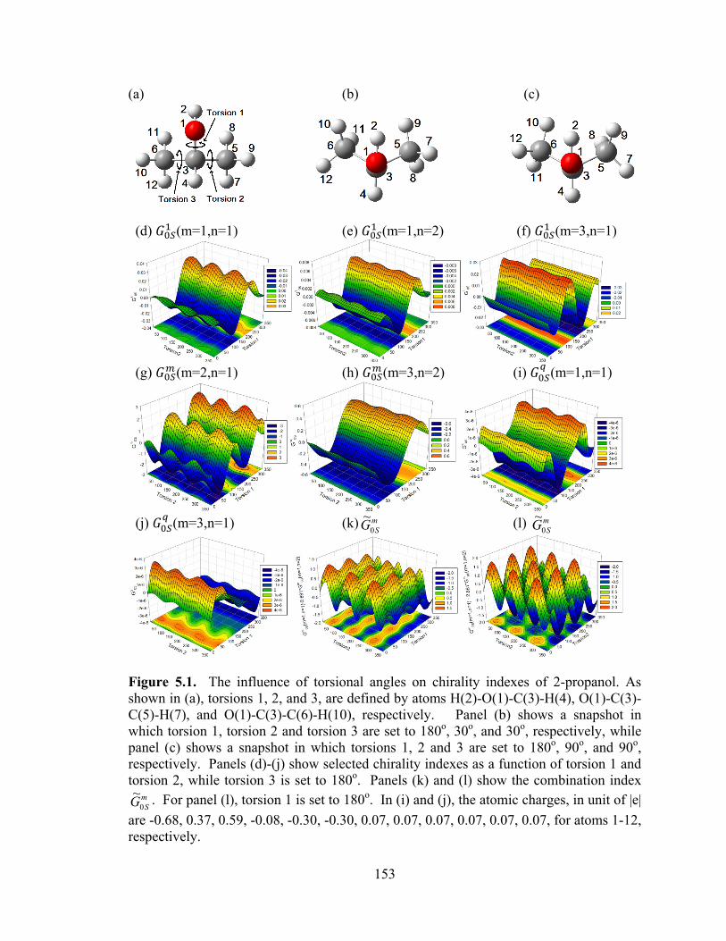
153

(a) (b) (c)

(d) (m=1,n=1) (e) (m=1,n=2) (f) (m=3,n=1)

(g) (m=2,n=1) (h) (m=3,n=2) (i) (m=1,n=1)

(j) (m=3,n=1) (k) m

SG0~ (l) m

SG0~

Figure 5.1. The influence of torsional angles on chirality indexes of 2-propanol. As shown in (a), torsions 1, 2, and 3, are defined by atoms H(2)-O(1)-C(3)-H(4), O(1)-C(3)-C(5)-H(7), and O(1)-C(3)-C(6)-H(10), respectively. Panel (b) shows a snapshot in which torsion 1, torsion 2 and torsion 3 are set to 180o, 30o, and 30o, respectively, while panel (c) shows a snapshot in which torsions 1, 2 and 3 are set to 180o, 90o, and 90o, respectively. Panels (d)-(j) show selected chirality indexes as a function of torsion 1 and torsion 2, while torsion 3 is set to 180o. Panels (k) and (l) show the combination index

mSG0

~ . For panel (l), torsion 1 is set to 180o. In (i) and (j), the atomic charges, in unit of |e| are -0.68, 0.37, 0.59, -0.08, -0.30, -0.30, 0.07, 0.07, 0.07, 0.07, 0.07, 0.07, for atoms 1-12, respectively.

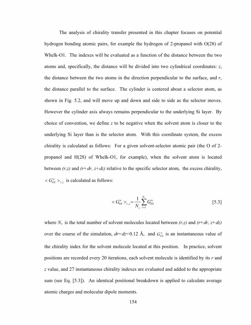
154

The analysis of chirality transfer presented in this chapter focuses on potential

hydrogen bonding atomic pairs, for example the hydrogen of 2-propanol with O(28) of

Whelk-O1. The indexes will be evaluated as a function of the distance between the two

atoms and, specifically, the distance will be divided into two cylindrical coordinates: z,

the distance between the two atoms in the direction perpendicular to the surface, and r,

the distance parallel to the surface. The cylinder is centered about a selector atom, as

shown in Fig. 5.2, and will move up and down and side to side as the selector moves.

However the cylinder axis always remains perpendicular to the underlying Si layer. By

choice of convention, we define z to be negative when the solvent atom is closer to the

underlying Si layer than is the selector atom. With this coordinate system, the excess

chirality is calculated as follows: For a given solvent-selector atomic pair (the O of 2-

propanol and H(28) of Whelk-O1, for example), when the solvent atom is located

between (r,z) and (r+dr, z+dz) relative to the specific selector atom, the excess chirality,

zrwSG ,0 >< is calculated as follows:

∑=

=><cN

i

wS

czr

wS G

NG

10,0

1

[5.3]

where Nc is the total number of solvent molecules located between (r,z) and (r+dr, z+dz)

over the course of the simulation, dr=dz=0.12 Å, and wSG0 is an instantaneous value of

the chirality index for the solvent molecule located at this position. In practice, solvent

positions are recorded every 20 iterations, each solvent molecule is identified by its r and

z value, and 27 instantaneous chirality indexes are evaluated and added to the appropriate

sum (see Eq. [5.3]). An identical positional breakdown is applied to calculate average

atomic charges and molecular dipole moments.

155

Figure 5.2. The cylindrical coordinate system used in the spatial breakdown of excess chirality, average atomic charges, and average solvent dipole. A chosen selector atom is placed at the center of the cylinder. Averages are collected over solvent molecules located between (r,z) and (r+dr,z+dz), where dr = dz = 0.12 Å. The cylinder axis is perpendicular to the underlying Si layer.

5.2.4 Simulation details

Surface-to-solvent chirality transfer is evaluated from molecular dynamics

simulations of the CSPs (Whelk-O1, DNB-leucine and DNB-phenylglycine) surrounded

by solvent. The solvent consists of either pure ethanol, pure 2-propanol, 80/20 n-

hexane/ethanol, or 80/20 n-hexane/2-propanol. The simulation cell, as shown in Fig.

2.10, has solvent confined between an upper and a lower surface that each include nine

selectors, end-caps, silanol groups and an underlying layer of Si. The full simulation cell

actually has empty space above the upper, and below the lower, surface such that roughly

2/3 of the entire cell is empty. 3D Periodic boundary conditions are applied in the

simulations and the space above and below the interfacial region minimizes interactions

between neighboring surface-fluid-surface slabs. The distance between the two

156

underlying Si layers is adjusted so that the solvent density in the center of the simulation

cell is close to the experimental density. Each simulation with pure solvent includes 600

solvent molecules, while each simulation with mixed solvents includes 400 solvent

molecules.

Electrostatic interactions are evaluated using Ewald summations, including a

correction for the rectangular prism shape of the simulation cell[40]. The results reported

below correspond to a momentum space cutoff of 272* ≤k and an Ewald parameter of

0.1916=α Å-1. The FC electrostatic interaction is incorporated into the Ewald

summations by replacing the Ewald forces for close intramolecular pairs of atoms where

Eq. [2.26] differs from the usual electrostatic potential.

Three Nosé-Hoover thermostats are used to generate canonical averages: one

thermostat is applied to translations; another is independently applied to rotations of the

rigid ring units in the selectors; and a third constrains the temperature associated with

charge fluctuations. The relevant conserved quantity in the simulations is defined by Eq.

[4.1] and has been described in detail in Chapter 4.

The initial configuration for the simulations is obtained by placing a large excess

of solvent molecules on a cubic lattice between the two surfaces and some are removed at

random until the desired number remain. Following this, the surface-to-surface distance

is increased until strong overlaps are removed. Then Monte Carlo cycles are performed

as the simulation cell is gradually recompressed. Finally, the molecules are assigned

random linear and angular velocities consistent with the desired temperature.

157

Simulations of 10-15 ns are performed for all twelve solvent-surface interfaces.

The time step for all simulations is 0.3 fs and the total change in the Nosé-Hoover

Hamiltonian, HNH, is 1% over 200 ps. The equilibration time of each simulation is 60 ps.

The duration of the equilibration period was decided based upon the dihedral

distributions of torsion 2 (O(1)-C(3)-C(5)-H(7)) for 2-propanol. Specifically, in the

starting structure of 2-propanol, torsion 2 is set to 60 degrees, and after 50 ps, we find

that it becomes equally distributed between the three isoenergetic conformers (60, 180,

and 270 degrees). In our previous work on chirality transfer about solutes[181], we

found that 4 ns was adequate to get converged results. The excess chirality reported in

this work has been averaged over the 18 selectors in the simulation cell, for a total

monitoring time of 180–270 ns.

The 2D solvent distribution about the chiral selectors, , ), is collected every

20 iterations along with chirality indexes, atomic charges, and molecular dipoles.

Snapshots of the entire simulation cell are collected every 5000 iterations. These

snapshots form the basis of the collection of hydrogen bonding statistics, where a

hydrogen bond is defined as X—H---Y, where X and Y are either O or N.

5.3. Results and discussion

The chirality transfer between surface and solvent is examined in this section for

the three CSPs, Whelk-O1, DNB-phenylglycine, and DNB-leucine, in the four solvents,

ethanol, 2-propanol, n-hexane/ethanol, n-hexane/2-propanol.

158

In our analysis of excess chirality, we place emphasis on solvent-to-selector

hydrogen bonding. Molecular dynamics simulations have been widely used to provide

detailed information on the spatial, energetic, and dynamic aspects of hydrogen bonds in

condensed phases [183-185]. Analyte-selector hydrogen bonding is invoked in many

CSP selective mechanisms[15] and simulations have successfully revealed the

importance of H-bonding for these selectors[161]. CH-π interactions are also included in

some CSP selectivity mechanisms[161, 186, 187] and will be noted below in regards to

chirality transfer to solvent.

5.3.1 Solvation of Chiral Stationary Phases

Before analyzing the selector-solvent chirality transfer, we begin with an analysis

of solvent structure about the stationary phases. 2D distributions are presented to show

solvent position, relative to specified selector atoms, as a function of distance along the

surface (r) and perpendicular to the surface (z). In the mixed solvents, results are shown

only for the alcohol component, since n-hexane does not interact strongly with the

selectors and prefers to be in the bulk. We also focus on the chirality transfer to alcohol

since it has the potential to hydrogen bond to the selectors and is most likely to be found

at the interface. Solvation studies for these selectors have been published elsewhere[112,

161], although not necessarily for the solvents of interest here.

H-bonding statistics for the three CSPs and the four solvents are presented in

Table 5.1. The probabilities in Table 5.1 are consistent with a previous study[112] of H-

bonding for DNB-phenylglycine and DNB-leucine, although they are consistently

somewhat lower. The selector representation is identical in both studies but a polarizable

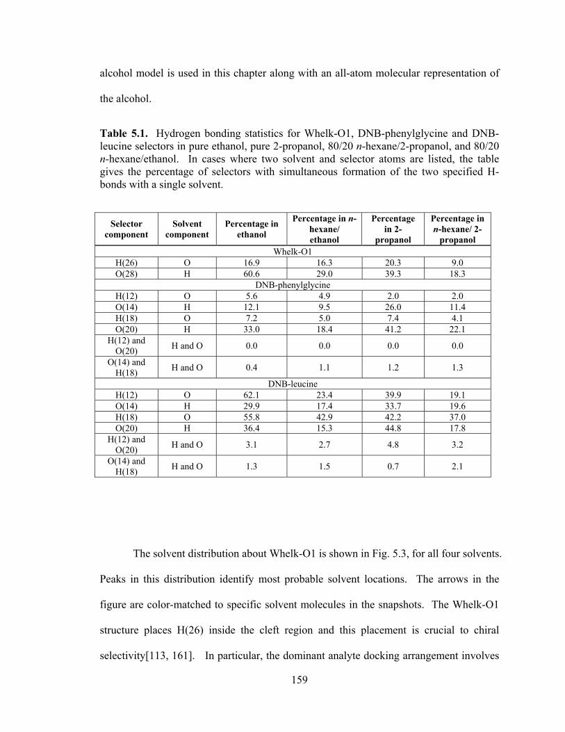
159

alcohol model is used in this chapter along with an all-atom molecular representation of

the alcohol.

Table 5.1. Hydrogen bonding statistics for Whelk-O1, DNB-phenylglycine and DNB-leucine selectors in pure ethanol, pure 2-propanol, 80/20 n-hexane/2-propanol, and 80/20 n-hexane/ethanol. In cases where two solvent and selector atoms are listed, the table gives the percentage of selectors with simultaneous formation of the two specified H-bonds with a single solvent.

Selector

component Solvent

component Percentage in

ethanol

Percentage in n-hexane/ ethanol

Percentage in 2-

propanol

Percentage in n-hexane/ 2-

propanol Whelk-O1

H(26) O 16.9 16.3 20.3 9.0 O(28) H 60.6 29.0 39.3 18.3

DNB-phenylglycine H(12) O 5.6 4.9 2.0 2.0 O(14) H 12.1 9.5 26.0 11.4 H(18) O 7.2 5.0 7.4 4.1 O(20) H 33.0 18.4 41.2 22.1

H(12) and O(20) H and O 0.0 0.0 0.0 0.0

O(14) and H(18) H and O 0.4 1.1 1.2 1.3

DNB-leucine H(12) O 62.1 23.4 39.9 19.1 O(14) H 29.9 17.4 33.7 19.6 H(18) O 55.8 42.9 42.2 37.0 O(20) H 36.4 15.3 44.8 17.8

H(12) and O(20) H and O 3.1 2.7 4.8 3.2

O(14) and H(18) H and O 1.3 1.5 0.7 2.1

The solvent distribution about Whelk-O1 is shown in Fig. 5.3, for all four solvents.

Peaks in this distribution identify most probable solvent locations. The arrows in the

figure are color-matched to specific solvent molecules in the snapshots. The Whelk-O1

structure places H(26) inside the cleft region and this placement is crucial to chiral

selectivity[113, 161]. In particular, the dominant analyte docking arrangement involves

160

H-bonding to H(26) and, as a result, any solvent in this region must be displaced by

analyte in order for chiral recognition to occur. Panels 4(a)-(d) show the 2D distribution

of the alcohol oxygen about H(26) in the four solvents. The ridge beginning at around

z=2Å, r=0 is due to direct solvent-selector H-bonding. The fact that this ridge occurs for

positive z clearly indicates that the solvent H-bonds from above (i.e. in the cleft). A

second ridge at somewhat higher z is also evident in the panels and this ridge is due to a

second solvent, within the cleft region, that is not directly H-bonded to the selector but

may H-bond to another solvent. The snapshots in panels (i)-(l) show these in-the-cleft

solvents. Solvent-selector H-bonding to the amide oxygen, O(28), occurs frequently and

this is evident from the prominence of the ridge at r=2Å in Panels (e)-(h). The solvent

prefers to place its hydrogen on the side of O(28), or closer to the surface as evident from

the shift in the peak position towards negative z. Thus, this solvent molecule is outside of

the cleft region and is less likely to interfere with chiral recognition.

The alcohol placement relative to the Whelk-O1 selector is similar for all four

solvents. Overall, 2-propanol is more likely to H-bond to H(26) and this is clear from the

stronger peak around z=2Å, r=0 in panels (c) and (d), relative to panels (a) and (b). The

2D distributions in panels (e)-(h) show that the H-bonding probability to O(28) is

comparable for ethanol and 2-propanol. The probability for secondary solvents, not

directly H-bonded to the selector, increases in 100% alcohol solvents. This is evident

from the prominent secondary ridges in 100% alcohol solvents (compare the z=4Å, r=0

ridge in Figs. 5.3(a) and 5.3(b) for example).

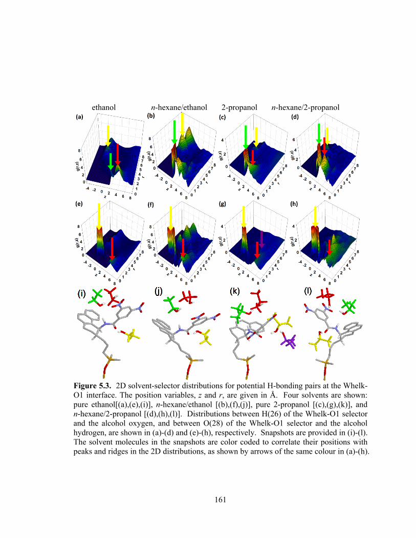
161

ethanol n-hexane/ethanol 2-propanol n-hexane/2-propanol

Figure 5.3. 2D solvent-selector distributions for potential H-bonding pairs at the Whelk-O1 interface. The position variables, z and r, are given in Å. Four solvents are shown: pure ethanol[(a),(e),(i)], n-hexane/ethanol [(b),(f),(j)], pure 2-propanol [(c),(g),(k)], and n-hexane/2-propanol [(d),(h),(l)]. Distributions between H(26) of the Whelk-O1 selector and the alcohol oxygen, and between O(28) of the Whelk-O1 selector and the alcohol hydrogen, are shown in (a)-(d) and (e)-(h), respectively. Snapshots are provided in (i)-(l). The solvent molecules in the snapshots are color coded to correlate their positions with peaks and ridges in the 2D distributions, as shown by arrows of the same colour in (a)-(h).

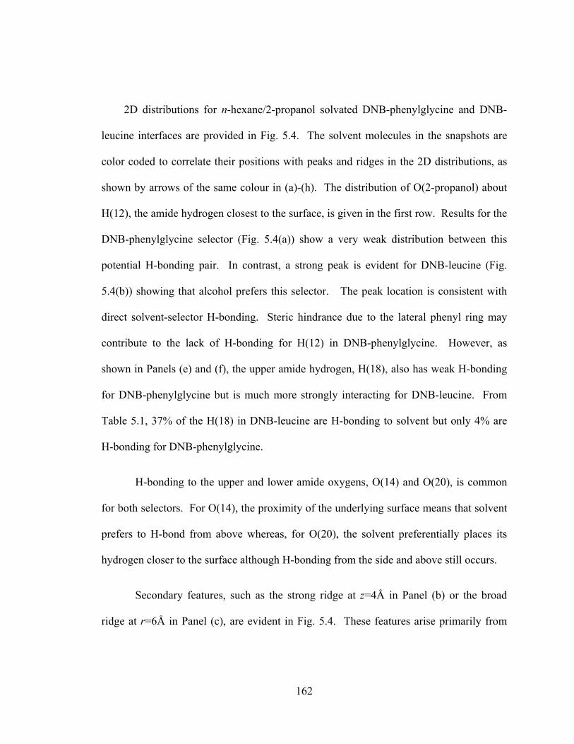
162

2D distributions for n-hexane/2-propanol solvated DNB-phenylglycine and DNB-

leucine interfaces are provided in Fig. 5.4. The solvent molecules in the snapshots are

color coded to correlate their positions with peaks and ridges in the 2D distributions, as

shown by arrows of the same colour in (a)-(h). The distribution of O(2-propanol) about

H(12), the amide hydrogen closest to the surface, is given in the first row. Results for the

DNB-phenylglycine selector (Fig. 5.4(a)) show a very weak distribution between this

potential H-bonding pair. In contrast, a strong peak is evident for DNB-leucine (Fig.

5.4(b)) showing that alcohol prefers this selector. The peak location is consistent with

direct solvent-selector H-bonding. Steric hindrance due to the lateral phenyl ring may

contribute to the lack of H-bonding for H(12) in DNB-phenylglycine. However, as

shown in Panels (e) and (f), the upper amide hydrogen, H(18), also has weak H-bonding

for DNB-phenylglycine but is much more strongly interacting for DNB-leucine. From

Table 5.1, 37% of the H(18) in DNB-leucine are H-bonding to solvent but only 4% are

H-bonding for DNB-phenylglycine.

H-bonding to the upper and lower amide oxygens, O(14) and O(20), is common

for both selectors. For O(14), the proximity of the underlying surface means that solvent

prefers to H-bond from above whereas, for O(20), the solvent preferentially places its

hydrogen closer to the surface although H-bonding from the side and above still occurs.

Secondary features, such as the strong ridge at z=4Å in Panel (b) or the broad

ridge at r=6Å in Panel (c), are evident in Fig. 5.4. These features arise primarily from

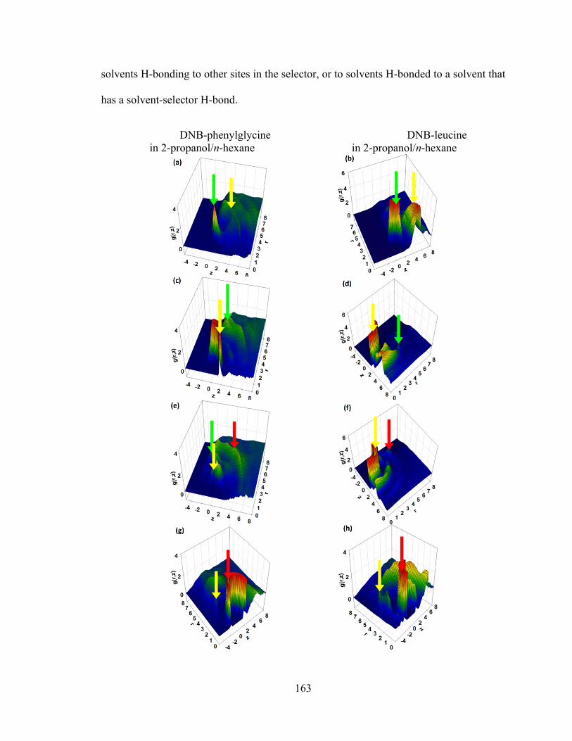
163

solvents H-bonding to other sites in the selector, or to solvents H-bonded to a solvent that

has a solvent-selector H-bond.

DNB-phenylglycine DNB-leucine in 2-propanol/n-hexane in 2-propanol/n-hexane

164

Figure 5.4. 2D distributions from 2-propanol/n-hexane solvated DNB-phenylglycine and DNB-leucine interfaces. The position variables, z and r, are given in Å. Each column refers to a specific stationary phase. Specifically, panels [(a),(c),(e),(g)] and [(b),(d),(f),(h)] show g(r,z) for DNB-phenylglycine and DNB-leucine, respectively. Corresponding snapshots are provided in Panels (i) and (j). The first, second, third, and fourth rows show the distribution between H(12)-O(2-propanol), O(14)-H(2-propanol), H(18)-O(2-propanol), and O(20)-H(2-propanol), respectively. The solvent molecules in the snapshots are color coded to correlate their positions with peaks and ridges in the 2D distributions, as shown by arrows of the same colour in (a)-(h).

2D distribution for 2-propanol, ethanol, and ethanol/n-hexane about DNB-

phenylglycine and DNB-leucine have not been shown but Table 5.1 provides H-bonding

statistics. Qualitatively, the 2D distributions are similar to those in Fig. 5.4 but there is a

more pronounced quantitative difference between DNB-leucine and DNB-phenylglycine

in an ethanol solvent. For DNB-phenylglycine, the overall number of ethanol-selector H-

bonds is less than for 2-propanol, and this is particularly true for the pure solvents. In

contrast, ethanol forms more H-bonds to DNB-leucine, on average, than does 2-propanol.

In order to correlate solvent position with chirality transfer, the 2D solvent

distributions shown in this section will be represented as contour plots in the subsequent

sections.

165

5.3.2 Chirality transfer at interfaces

The alcohol molecules at the interface necessarily explore a broad range of

conformations. The excess chirality of interest here results from a small imbalance in the

conformational distributions resulting from the chiral environment. It follows that some

estimation of the accuracy of the predicted chirality transfers is required. Fig. 5.5

provides a selection of excess chiralities for 2-propanol in 2-propanol/n-hexane solvated

DNB-phenylglycine and DNB-leucine.

The panels in Fig. 5.5, and in all subsequent presentations of excess chirality, use

color coding to identify regions where the excess chirality is negative (blue, indigo)

versus regions where it is positive (yellow, orange, red). Green indicates an average

close to zero. In the panels, green is also used for regions where solvent is rarely found:

We require a minimum of 20000 instantaneous chiralities recorded before presenting an

excess chirality for the region. In practice, the solvent is rarely found within the end cap

region for steric reasons. In higher probability regions, such as H-bonding areas, the

number of instantaneous chirality indexes normally exceeds 200,000. Overlaid on the

maps of chirality transfer are contour maps that show the 2D probability distributions

analogous to Figs. 5.3 and 5.4. In this way, with color coded maps and contour plots, one

can correlate regions of high solvent density with regions of high chirality transfer.

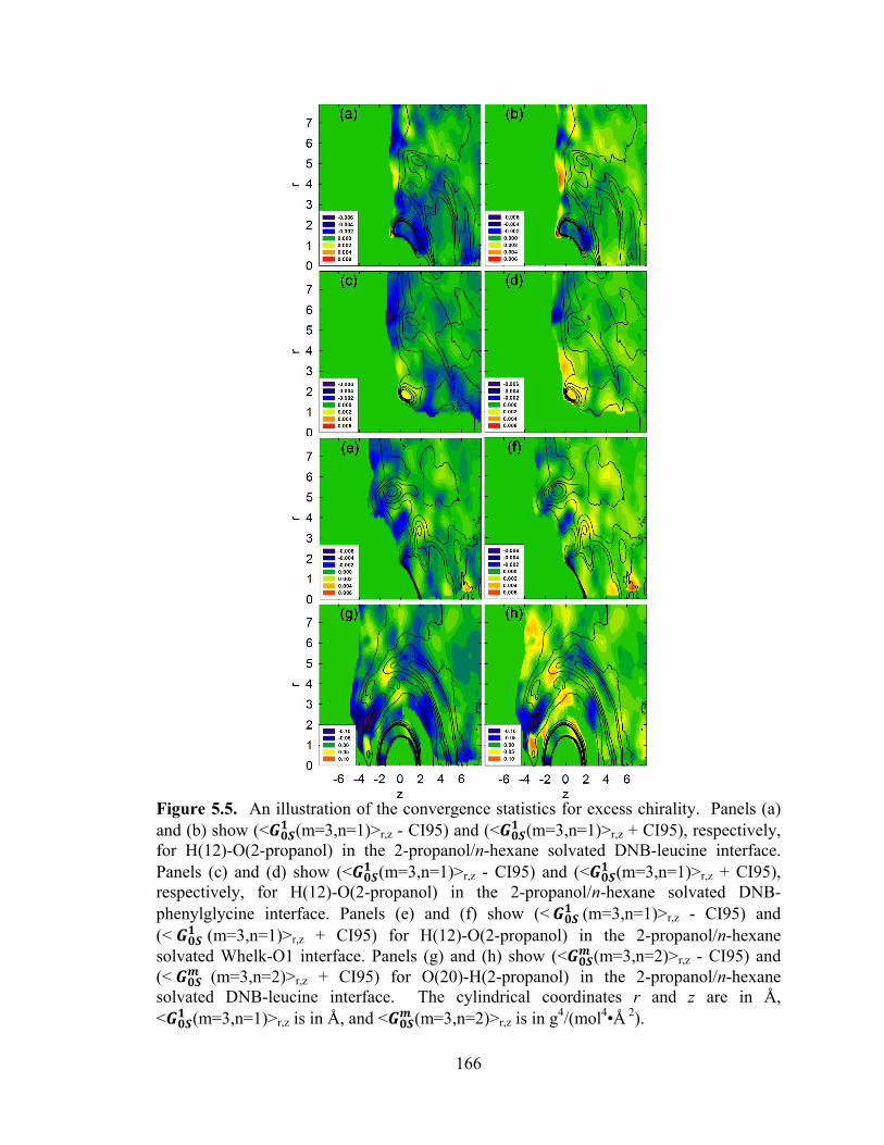
166

Figure 5.5. An illustration of the convergence statistics for excess chirality. Panels (a) and (b) show (< (m=3,n=1)>r,z - CI95) and (< (m=3,n=1)>r,z + CI95), respectively, for H(12)-O(2-propanol) in the 2-propanol/n-hexane solvated DNB-leucine interface. Panels (c) and (d) show (< (m=3,n=1)>r,z - CI95) and (< (m=3,n=1)>r,z + CI95), respectively, for H(12)-O(2-propanol) in the 2-propanol/n-hexane solvated DNB-phenylglycine interface. Panels (e) and (f) show (< (m=3,n=1)>r,z - CI95) and (< (m=3,n=1)>r,z + CI95) for H(12)-O(2-propanol) in the 2-propanol/n-hexane solvated Whelk-O1 interface. Panels (g) and (h) show (< (m=3,n=2)>r,z - CI95) and (< (m=3,n=2)>r,z + CI95) for O(20)-H(2-propanol) in the 2-propanol/n-hexane solvated DNB-leucine interface. The cylindrical coordinates r and z are in Å, < (m=3,n=1)>r,z is in Å, and < (m=3,n=2)>r,z is in g4/(mol4•Å 2).

167

The rightmost panels in Fig. 5.5 show , minus the 95% confidence interval

(CI95). The leftmost panels show , plus the CI95, which is calculated from[188]

⎟⎠⎞⎜

⎝⎛ −=

2

,0,

20 )(96.195

zr

wSzr

wS

c

GGN

CI [5.4]

where Nc is the number of solvent molecules located between (r, z) and (r+dr, z+dz)

about the selector atom during the collection period of the simulation. In calculating

CI95, a Gaussian distribution is assumed. Regions of consistent color coding between

the right and left panels indicate good statistics. Notice that the color coding is similar in

many regions on both panels, and particularly regions of high solvent density, where the

error is generally small relative to the overall magnitude of the excess chirality. The

largest errors tend to occur for regions of low solvent density, where there are fewer

values of the chirality index recorded, and for small r values, due to a smaller collection

volume, leading to a reduction of counts.

Before proceeding to a detailed analysis of the chirality transfer, it is worth noting

the scale of the chirality transfers in Fig. 5.5. For 3, 1 , , the excess

chirality induced in 2-propanol can be up-to 20% of the maximum value observed in Fig.

5.1(f). Thus, there is cancellation between instantaneous chirality indexes but the

residual remains significant. Likewise, the average value of 3, 2 , can

reach up-to 17% of the maximum value. These excess chiralities are much larger than

were observed in Chapter 4, where solutes in the bulk were considered. As expected, the

immobilization of the chiral selectors onto a surface, and possibly the collective effect of

multiple selectors, has lead to a significant chirality transfer into nearby solvents.

168

5.3.3 Comparisons between selectors: Conformational chirality

In this section, we analyze the chirality transfer to 2-propanol, in the binary 2-

propanol/n-hexane solvent, when this solvent is near a DNB-leucine, DNB-phenylglycine,

or Whelk-O1 interface. In this section, we focus on characterizing conformational bias

introduced into the solvent molecules. Solvent polarization due to the chiral interface

will be examined in Section 5.3.4 and comparisons between different solvents will be

presented in Section 5.3.5.

Fig. 5.6 presents , , , , and , , collected around the H-bonding

sites (H(12), O(14), H(18), O(20)) of the DNB-leucine selector. The cylindircal

coordinates r and z are in Å, < (m=3,n=1)>r,z is in Å, and < (m=3,n=2)>r,z is in

g4/(mol4•Å 2). H(12) is closest to the underlying surface, and H-bonding imposes steric

constraints on the solvent. This solvent is often located on the same side as the lateral

isopropyl group of the selector, as shown in the snapshot 5.6(d), which introduces

additional steric constraints. Both , and , are strongly dependent on

Torsion 1, defined by H(2)-O(1)-C(3)-H(4), which orients the alcohol hydrogen relative

to the rest of the molecule. Figs. 5.6(a) and 5.6(b) show a significant negative excess

chirality for 2-propanol in the high probability region where direct H-bonding to H(12)

occurs. One can extract from Fig. 5.1 that simultaneous negative average values for these

two indexes means a bias in Torsion 1 towards values between 0 and 60 degrees, where

the alcohol hydrogen is gauche to the methine hydrogen. The snapshot in Fig. 5.6(d)

provides an illustration of this solvent configuration (Torsion 1 = 48 degrees in the

snapshot) .

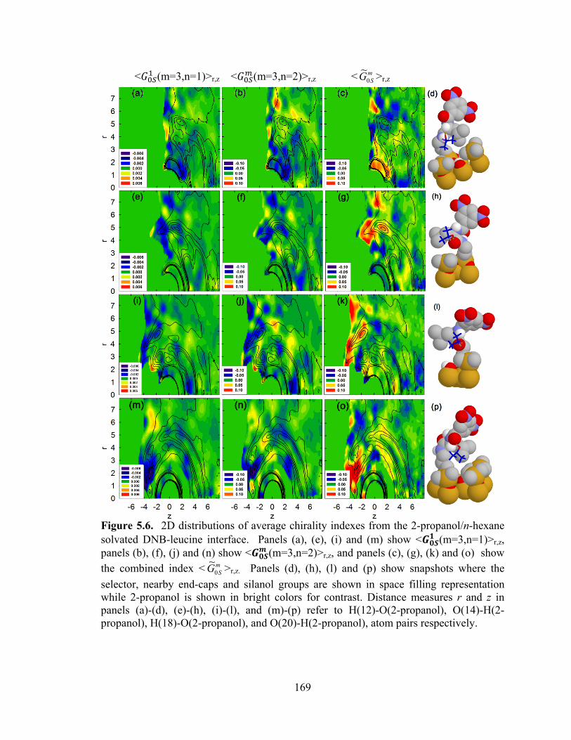
169

< (m=3,n=1)>r,z < (m=3,n=2)>r,z < mSG0

~ >r,z

Figure 5.6. 2D distributions of average chirality indexes from the 2-propanol/n-hexane solvated DNB-leucine interface. Panels (a), (e), (i) and (m) show < (m=3,n=1)>r,z, panels (b), (f), (j) and (n) show < (m=3,n=2)>r,z, and panels (c), (g), (k) and (o) show the combined index < m

SG0~ >r,z. Panels (d), (h), (l) and (p) show snapshots where the

selector, nearby end-caps and silanol groups are shown in space filling representation while 2-propanol is shown in bright colors for contrast. Distance measures r and z in panels (a)-(d), (e)-(h), (i)-(l), and (m)-(p) refer to H(12)-O(2-propanol), O(14)-H(2-propanol), H(18)-O(2-propanol), and O(20)-H(2-propanol), atom pairs respectively.

170

Hydrogen bonding to the upper amide hydrogen, H(18), is distinct from the lower

amide hydrogen, as shown in Panels 5.6(i) and 5.6(j). First, the H-bonding solvent

adopts a wider range of positions and may even be closer to the surface than H(18).

Consistent with the greater positional freedom allowed to the solvent, the excess chirality

for H-bonding solvent is generally small indicating significant conformational freedom as

well. However, there is an indication of some excess chirality around z=-1.0Å, when the

solvent is positioned close to the surface while maintaining an H-bond with H(18). A

closer inspection of solvents in this location indicates that a non-negligible fraction

simultaneously form two H-bonds to the selector, one to O(14) and one to H(18). This

forces the alcohol group to point towards the underlying surface, and one methyl group

points towards the bulk. The spatial constraints of forming two H-bonds, coupled with

steric constraints from the selector lateral group and the underlying surface, lead to a

negative excess chirality in this case.

According to Table 5.1 20% of the DNB-leucine selectors have H-bonds to O(14),

but these solvents do not have significant excess chirality for several reasons. First, the

solvent has some positional flexibility and can H-bond from above or slightly below

O(14). Second, the solvent often adopts a position opposite, or tangential to, the lateral

group. These factors indicate minimal steric constraints and lead to small excess chirality.

It is interesting to note that dual H-bonding with H(18), as discussed in the preceding

paragraph, has a smaller contribution for O(14). This follows because these multiple H-

bonding solvents tend to occupy positions relative to O(14) that also occur much more

frequently for solvents with a single H-bond to the selector.

171

H-bonding to O(20) is generally characterized by small-to-negligible chirality

transfer except for solvents located closer to the underlying surface (ridge ending around

z=-2Å in Figs. 5.6(m) and 5.6(n)). Upon close inspection of the corresponding snapshots,

we find that a significant fraction of solvents at this location simultaneously form an H-

bond to H(12). This forces the alcohol group to point towards the bulk, and one methyl

group points towards the underlying surface. On average, these 2-propanol molecules

have the methine H and the alcohol H in a gauche configuration, leading to an overall

negative excess chirality. Overall, H-bonding to the amide oxygens is probable (see

Table 5.1) but is not accompanied by significant chirality transfer to solvent. In contrast,

H-boding to the amide hydrogens can be accompanied by steric or energetic constraints

that lead to significant excess chiralities.

Panels 5.6(c), 5.6(g), 5.6(k), and 5.6(o) show , , the combination index

introduced to isolate the contribution of methyl torsions. Overall, this index is negligible

in regions where , and , are small, indicating that “unbiased” solvent

conformational averaging occurs in these cases and chirality transfer is small-to-

negligible. The largest values of , occur for solvent H-bonding to H(12) and

the excess , is significantly positive. By reference to Figs. 5.1(k) and 5.1(l),

this indicates that the methyl groups prefer to orient such that a hydrogen is cis-to-gauche

relative to the alcohol oxygen.

Hydrogen bonding to the backbone of DNB-phenylglycine occurs less frequently

than for DNB-leucine, as shown in Table 5.1. This is particularly true for the amide

hydrogens, where only 2-4% of the selectors have H-bonding to these atoms. The

172

occurrence of simultaneous multiple H-bonds is also less common for DNB-

phenylglycine due to the bulky lateral group and a small number of energetically

accessible backbone conformations. The lateral phenyl ring impacts excess solvent

chirality in two ways. First, CH-π interactions will encourage certain energy lowering

solvent positions and orientations. On the other hand, the ring imposes steric constraints

when the solvent is too close and this may bias towards specific conformations.

The excess solvent chirality for 2-propanol in 2-propanol/n-hexane about DNB-

phenylglycine is shown in Fig. 5.7. The cylindircal coordinates r and z are in Å,

< (m=3,n=1)>r,z is in Å, and < (m=3,n=2)>r,z is in g4/(mol4•Å 2). Panels (a) and (b)

show a positive excess chirality introduced in 2-propanol molecules that H-bond to H(12)

of DNB-phenylglycine (see z=0, r=2Å region). This is in direct contrast to DNB-leucine

where solvent hydrogen bonded to H(12) has a negative excess chirality: The change in

lateral group has reversed the conformational bias of the nearby solvent. For the other H-

bonding atoms (O(14), H(18), and O(20)) of DNB-phenylglycine, a negative excess

chirality is induced for a localized subset of the H-bonding solvent. For example,

chirality transfer for solvent H-bonded to O(14) is generally small except when the

solvent is closer to the underlying surface.

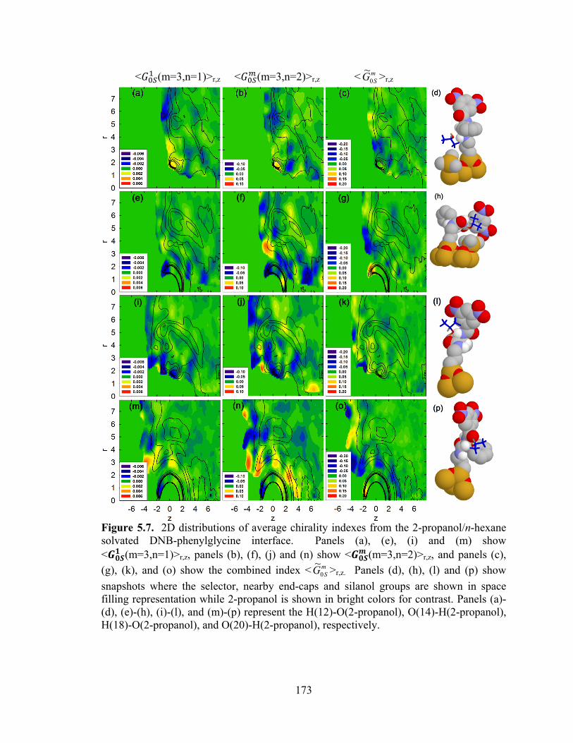
173

< (m=3,n=1)>r,z < (m=3,n=2)>r,z < mSG0

~ >r,z

Figure 5.7. 2D distributions of average chirality indexes from the 2-propanol/n-hexane solvated DNB-phenylglycine interface. Panels (a), (e), (i) and (m) show < (m=3,n=1)>r,z, panels (b), (f), (j) and (n) show < (m=3,n=2)>r,z, and panels (c), (g), (k), and (o) show the combined index < m

SG0~ >r,z. Panels (d), (h), (l) and (p) show

snapshots where the selector, nearby end-caps and silanol groups are shown in space filling representation while 2-propanol is shown in bright colors for contrast. Panels (a)-(d), (e)-(h), (i)-(l), and (m)-(p) represent the H(12)-O(2-propanol), O(14)-H(2-propanol), H(18)-O(2-propanol), and O(20)-H(2-propanol), respectively.

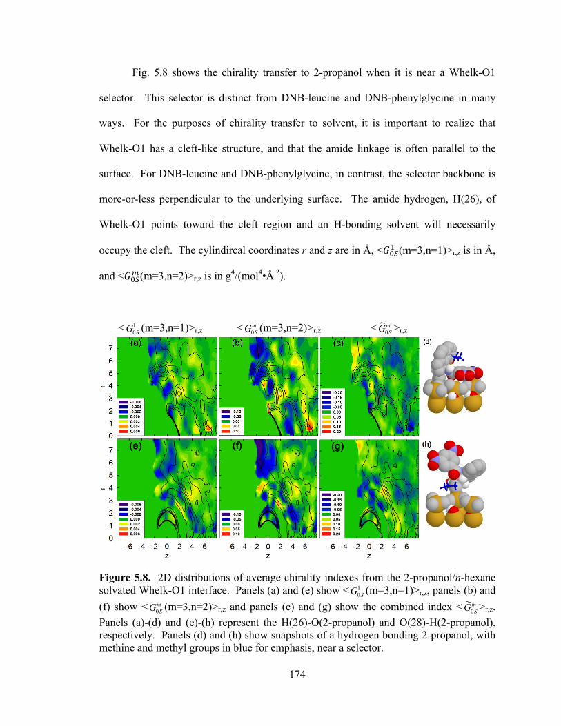
174

Fig. 5.8 shows the chirality transfer to 2-propanol when it is near a Whelk-O1

selector. This selector is distinct from DNB-leucine and DNB-phenylglycine in many

ways. For the purposes of chirality transfer to solvent, it is important to realize that

Whelk-O1 has a cleft-like structure, and that the amide linkage is often parallel to the

surface. For DNB-leucine and DNB-phenylglycine, in contrast, the selector backbone is

more-or-less perpendicular to the underlying surface. The amide hydrogen, H(26), of

Whelk-O1 points toward the cleft region and an H-bonding solvent will necessarily

occupy the cleft. The cylindircal coordinates r and z are in Å, < (m=3,n=1)>r,z is in Å,

and < (m=3,n=2)>r,z is in g4/(mol4•Å 2).

< 1

0SG (m=3,n=1)>r,z < mSG0 (m=3,n=2)>r,z < m

SG0~ >r,z

Figure 5.8. 2D distributions of average chirality indexes from the 2-propanol/n-hexane solvated Whelk-O1 interface. Panels (a) and (e) show < 1

0SG (m=3,n=1)>r,z, panels (b) and (f) show < m

SG0 (m=3,n=2)>r,z and panels (c) and (g) show the combined index < mSG0

~ >r,z. Panels (a)-(d) and (e)-(h) represent the H(26)-O(2-propanol) and O(28)-H(2-propanol), respectively. Panels (d) and (h) show snapshots of a hydrogen bonding 2-propanol, with methine and methyl groups in blue for emphasis, near a selector.

175

Fig. 5.3(a), and the contour plots in Figs. 5.8(a)-(c), reflect that there are multiple

solvents in the cleft region: an alcohol that H-bonds to H(26) directly and additional

solvent. The snapshot in Fig. 5.8(d) shows a typical solvent H-bonding to H(26), and the

excess chiralities in Panels (a) and (b) are weakly positive for this solvent in this region,

indicating that the alcohol H prefers to orient towards the methyl on the left (see Fig.

5.1(a)). Other in-the-cleft solvents appear at slightly larger separations from H(26) and

the simulations show that the chirality transfer to these solvent molecules is significant

and, depending on solvent position, the alcohol hydrogen is oriented away from the

methyls. From the perspective of chirality transfer, both in-the-cleft solvents experience

a significant but distinct conformational imbalance due to the nearby chiral selector.

Hydrogen bonding to O(28) of Whelk-O1 occurs primarily from the side, as noted

previously. Regardless of solvent position, this solvent is not in the cleft region, nor is it

typically close to the aromatic regions of the selector. Thus, it is the proximity of the end

caps that plays the largest steric role. Consistent with this, the excess chirality varies as a

function of the solvent distance from the underlying surface. Panel 5.7(h) shows a typical

solvent, and the steric constraints due to the nearby end-caps are evident.

5.3.4 Comparisons between selectors: Solvent polarization

Solvent molecules in the vicinity of a chiral selector will respond by biasing

towards certain conformations, as discussed in Section 5.3.3. In addition, the solvent will

become polarized as the electrons respond to the local chiral environment. Although our

molecular dynamics simulations are classical, the alcohol models are polarizable and

parameterized based on molecular response to electric fields. In this section, we examine

176

average atomic charges, and dipole moments for alcohol in the vicinity of the chiral

selectors.

Fig. 5.9 shows simulation results for 2-propanol, in a 2-propanol/n-hexane solvent,

near a DNB-leucine interface. It is immediately clear from Fig. 5.9 that the atomic

charges of the oxygen and hydrogen decrease, along with the dipole moment, for solvent

near the selector. Thus proximity to the interface is accompanied by a reduction in

solvent polarity. The bulk is primarily n-hexane, with occasional clusters of 2-propanol

molecules. Within these clusters, alcohol-to-alcohol H-bonding occurs. The shift

towards lower polarity at the interface indicates that H-bonding between 2-propanol

molecules is more polarizing than the alcohol-DNB-leucine interaction, even when the

alcohol H-bonds directly to the selector.

The dipole moment shows more variation with solvent location than the atomic

charges. Solvent hydrogen bonded to H(12), for example, has an average oxygen charge

of around -0.85 |e| and an average hydrogen charge between 0.45 |e| and 0.50 |e| . In

contrast, the dipole moment varies from 2.2 to 2.5 Debye. The variation in the dipole

moment reflects conformational changes as well as changes in atomic charges.

Unfortunately, this conformational effect can occur in the absence of chirality. For

instance, ab initio calculations indicate that the gas phase molecular dipole of 2-propanol

is 1.67 D when torsion 1 is 180 degrees, but is 1.58 D when this torsion is 60 degrees or

300 degrees. A shift towards the latter angles, without biasing towards either one, will

decrease the dipole but not introduce chirality.

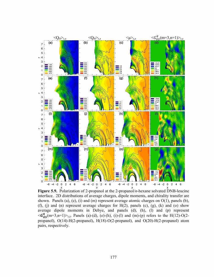
177

<QO>r,z <QH>r,z <μ>r,z < (m=3,n=1)>r,z

Figure 5.9. Polarization of 2-propanol at the 2-propanol/n-hexane solvated DNB-leucine interface. 2D distributions of average charges, dipole moments, and chirality transfer are shown. Panels (a), (e), (i) and (m) represent average atomic charges on O(1), panels (b), (f), (j) and (n) represent average charges for H(2), panels (c), (g), (k) and (o) show average dipole moments in Debye, and panels (d), (h), (l) and (p) represent < (m=3,n=1)>r,z. Panels (a)-(d), (e)-(h), (i)-(l) and (m)-(p) refers to the H(12)-O(2-propanol), O(14)-H(2-propanol), H(18)-O(2-propanol), and O(20)-H(2-propanol) atom pairs, respectively.

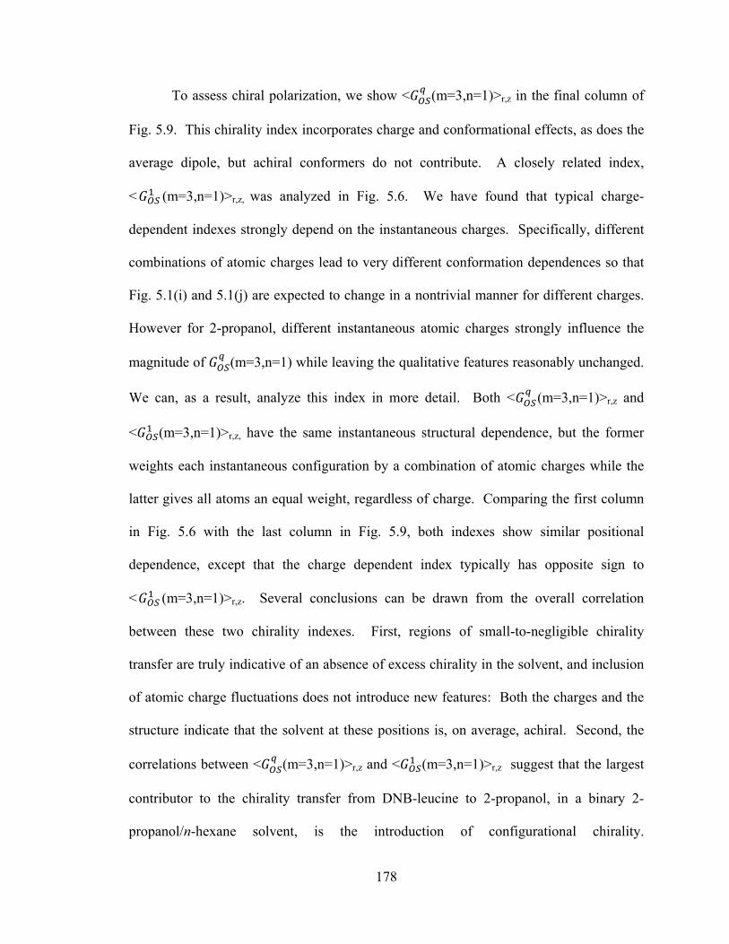
178

To assess chiral polarization, we show < (m=3,n=1)>r,z in the final column of

Fig. 5.9. This chirality index incorporates charge and conformational effects, as does the

average dipole, but achiral conformers do not contribute. A closely related index,

< (m=3,n=1)>r,z, was analyzed in Fig. 5.6. We have found that typical charge-

dependent indexes strongly depend on the instantaneous charges. Specifically, different

combinations of atomic charges lead to very different conformation dependences so that

Fig. 5.1(i) and 5.1(j) are expected to change in a nontrivial manner for different charges.

However for 2-propanol, different instantaneous atomic charges strongly influence the

magnitude of (m=3,n=1) while leaving the qualitative features reasonably unchanged.

We can, as a result, analyze this index in more detail. Both < (m=3,n=1)>r,z and

< (m=3,n=1)>r,z, have the same instantaneous structural dependence, but the former

weights each instantaneous configuration by a combination of atomic charges while the

latter gives all atoms an equal weight, regardless of charge. Comparing the first column

in Fig. 5.6 with the last column in Fig. 5.9, both indexes show similar positional

dependence, except that the charge dependent index typically has opposite sign to

< (m=3,n=1)>r,z. Several conclusions can be drawn from the overall correlation

between these two chirality indexes. First, regions of small-to-negligible chirality

transfer are truly indicative of an absence of excess chirality in the solvent, and inclusion

of atomic charge fluctuations does not introduce new features: Both the charges and the

structure indicate that the solvent at these positions is, on average, achiral. Second, the

correlations between < (m=3,n=1)>r,z and < (m=3,n=1)>r,z suggest that the largest

contributor to the chirality transfer from DNB-leucine to 2-propanol, in a binary 2-

propanol/n-hexane solvent, is the introduction of configurational chirality.

179

< (m=3,n=1)>r,z includes contributions from configurations and charge distributions.

The similarity between < (m=3,n=1)>r,z and < (m=3,n=1)>r,z shows that the charge

distributions have a secondary impact in this case.

Although Fig. 5.9 shows the polarization induced in 2-propanol due to a nearby

DNB-leucine interface, very similar changes in the solvent are observed for a DNB-

phenylglycine interface. Similar conclusions also follow from an analysis of the

polarization induced by the Whelk-O1 selector. However, it is interesting to note that,

for in-the-cleft solvents, the solvent that H-bonds to H(26) has reduced atomic charges

and dipole moment. In contrast, other in-the-cleft solvents have charges and dipole

moments consistent with molecules in the bulk.

5.3.5 Comparison of different solvents

In this section, we focus on the changes in excess chirality when the solvent

composition changes from pure alcohol to alcohol/alkane. In practice, normal phase

chiral separations tend to have varying amounts of alcohol in a predominantly nonpolar

(typically n-hexane) solvent. The analysis in this section will provide some indication of

the changes in the alcohol due to the presence of a co-solvent.

Fig. 5.10 provides several chirality indexes, atomic charges, and the dipole

moment for alcohol in the vicinity of the amide hydrogen, H(26), of Whelk-O1. Four

solvent environments are compared and the trends are representative of those observed

for the other CSPs. The spatial extent of the excess chirality is evident from the panels in

Fig. 5.10. First, chirality transfer to the alcohol is larger and persists further into the bulk

in an alcohol/alkane solvent than in a pure alcohol solvent. Both solvent environments

180

are fundamentally different and, from our results, the extensive hydrogen bonding

network in a 100% alcohol solvent diminishes the selector-to-solvent chirality transfer,

both in terms of magnitude and extent. In an alcohol/alkane solvent, the alcohols interact

individually with a selector or, at best have one or two nearby alcohols. Thus, the alcohol

molecule in this solvent has fewer opportunities to form H-bonds and this increases the

impact of the chiral selectors at the surface. In general, the range of the chirality transfer

into 2-propanol/n-hexane is larger than for ethanol/n-hexane: 2-propanol is larger and

will be more susceptible to sterically induced chirality transfer from the selector.

The absence of an alkane co-solvent may also impact the details of the chirality

transfer. This in not particularly evident for H(26) of Whelk-O1 but, for DNB-leucine

and DNB-phenylglycine, the excess chirality may change signs in certain regions around

the selector. For example, when ethanol H-bonds to the upper amide oxygen, O(20), of

DNB-leucine, the chirality transfer is weakly positive for an ethanol/n-hexane solvent but

negative in a pure ethanol solvent.

Panels 5.10(e) and 5.10(i) show that the charge on oxygen and on hydrogen are

smaller in magnitude for solvent near the surface and that the decrease is reasonably

systematic. This is particularly true for pure alcohol, as evident from the strong z

dependence of the charges shown in panels (f), (h),(j), and (l). This decrease in charge

occurs regardless of the solvent environment and, overall, the atomic charges are roughly

10-15% smaller near the surface, relative to the bulk. As expected, the dipole moment

also decreases but by a somewhat larger 15-25%. As noted in Section 5.3.3, this

contribution does not necessarily result from chirality and this is clear when the relatively

featureless < (m=3,n=1)>r,z is examined for the pure alcohols (Panels (n) and (p)).

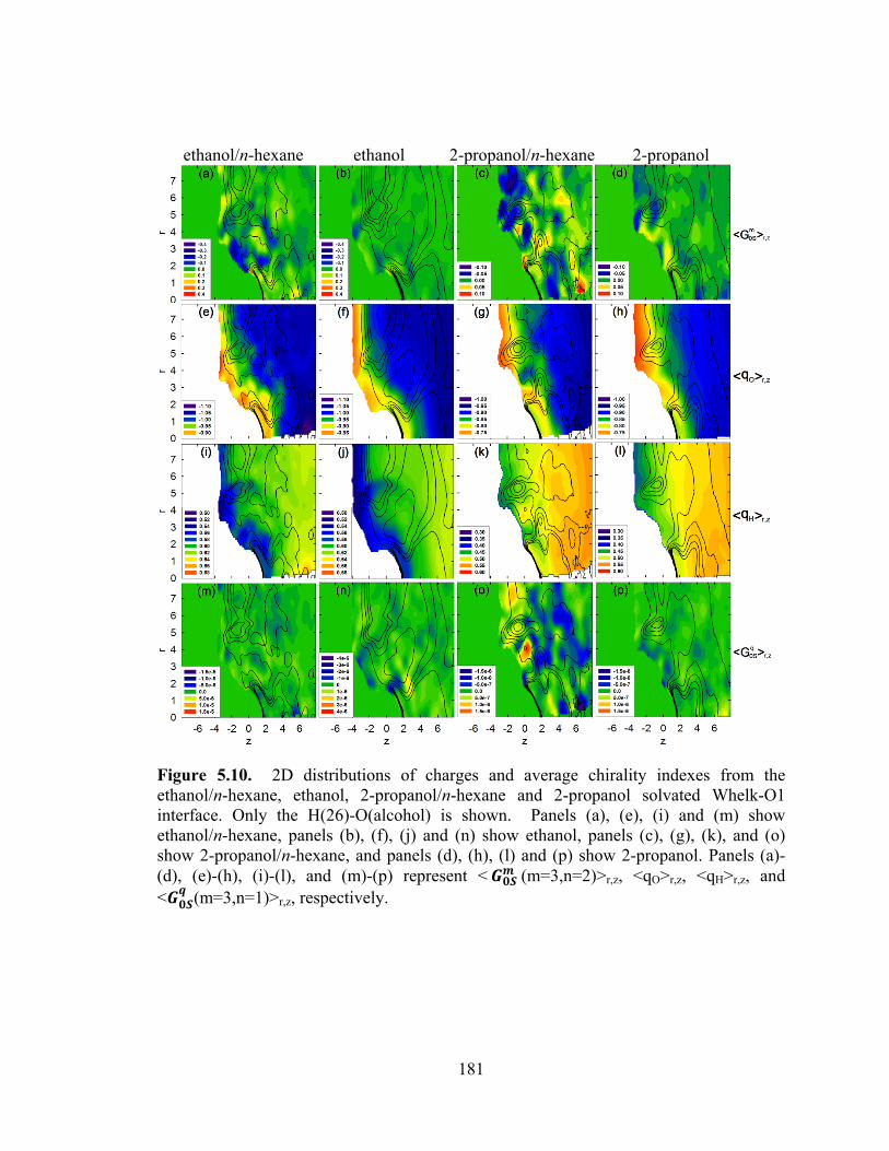
181

ethanol/n-hexane ethanol 2-propanol/n-hexane 2-propanol

Figure 5.10. 2D distributions of charges and average chirality indexes from the ethanol/n-hexane, ethanol, 2-propanol/n-hexane and 2-propanol solvated Whelk-O1 interface. Only the H(26)-O(alcohol) is shown. Panels (a), (e), (i) and (m) show ethanol/n-hexane, panels (b), (f), (j) and (n) show ethanol, panels (c), (g), (k), and (o) show 2-propanol/n-hexane, and panels (d), (h), (l) and (p) show 2-propanol. Panels (a)-(d), (e)-(h), (i)-(l), and (m)-(p) represent < (m=3,n=2)>r,z, <qO>r,z, <qH>r,z, and < (m=3,n=1)>r,z, respectively.

182

5.4. Conclusions

In this chapter, the impact of a nearby chiral surface on solvent is explored.

Emphasis is placed on evaluating the extent and characteristics of chirality transferred

from the surface to the solvent. The spatial characteristics of this chirality transfer, and

its dependence on the nature of the surface and solvent are examined in detail. Molecular

dynamics simulations of the solvated chiral interfaces form the basis of the analysis. The

chirality induced in the solvent is assessed based on a broad series of related chirality

indexes, and combinations of indexes are also employed to isolate specific contributions,

such as individual torsions. Three surfaces, employed in chiral chromatography, are

considered: The Whelk-O1 interface; a phenylglycine-derived CSP; and a leucine-

derived CSP. The solvents consist of ethanol, a binary n-hexane/ethanol solvent, 2-

propanol, and a binary n-hexane/2-propanol solvent. Our results show that chirality

transfer is significantly larger at an interface, relative to the transfers observed for chiral

solutes in Chapter 4.

The excess chirality is divided into two contributions, a conformational chirality

and a polarization contribution. Strictly speaking, these two factors are interrelated and

cannot be fully separated. However, with the use of appropriate chirality indexes, we can

emphasize the individual contributions. Our simulations reveal that solvents H-bonded to

the selectors have reduced atomic charges and reduced dipole moments. While the latter

is interesting, it does not necessarily follow from a selector-to-solvent chirality transfer:

conformational changes can alter the dipole but a conformational bias is required for

183

chirality transfer. Chirality indexes suggest that conformational chirality is dominant at

these interfaces, with solvent polarization having a smaller secondary effect.

A detailed analysis of conformational chirality reveals that the chirality transfer is

largest when the solvent experiences steric constraints or, alternatively, when the solvent

forms multiple interactions with the selector. The latter occurs via multiple hydrogen

bonds or CH-π interactions. In the absence of these constraints, the chirality transfer is

small, as exemplified by the minimal chirality transferred to 2-propanol when it H-bonds

to a carbonyl oxygen of DNB-leucine or DNB-phenylglycine. We find that the excess

chirality is attributable to local factors and that collective effects, due to the chiral field of

multiple selectors, appear to be minimal.

Chirality transfer is more significant and persists to larger distances away from

the selector in an alcohol/alkane solvent relative to a pure alcohol solvent. In addition,

the spatial range over which the chirality transfer is significant is typically larger for 2-

propanol than for ethanol, due mostly to additional steric constraints for the former.

184

Chapter 6 Conclusions The main objective of this thesis is to examine chirality transfer from chiral solutes and

surfaces to achiral solvents. Ab initio calculations are applied to develop polarizable

models and intramolecular potentials for solvents and solutes, and MD simulations are

used to study the induced chirality in achiral solvents. Five solvents (ethanol, 2-propanol,

benzyl-alcohol, ethanol/n-hexane, and 2-propanol/n-hexane), three solutes (PAMD,

acenaphthenol and styrene oxide) and three chiral surface selectors (Whelk-O1, DNB-

phenylglycine and DNB-leucine) are the focus of this study.

The methodology for developing a new polarizable and flexible model (the

fCINTRA model) is discussed in Chapter 3. In this methodology, the direct coupling

between polarization and intramolecular motion, such as bends and torsions, is novel.

The methodology integrates the FC method, field-dependent intramolecular potentials,

new equations of motion, damping functions for outside-of-range fields, and a reversible

multiple time step algorithm. The development of the field-dependent intramolecular

potentials of the fCINTRA model relies heavily on extensive ab initio calculations that

generate information on the molecule’s responses to various external electrostatic fields.

This methodology has been applied to ethanol as a test case.

MD simulations of bulk ethanol using the fCINTRA model are performed and the

physical properties, such as the self-diffusion coefficient, are assessed to evaluate the

quality of the model. Comparisons with other models show that the average dipole

moment of liquid ethanol predicted by the fCINTRA model is in closest agreement with

185

experiments and ab initio simulation results. The dielectric constant, interatomic

distributions and the enthalpy of vaporization are also in close agreement with

experiments. Self-diffusion is overestimated by the fCINTRA model, but it has been

found that the diffusion coefficient is highly sensitive to the fictitious charge mass and

further improvements could be made by reducing the mass. H-bonding analysis with the

fCINTRA model predicts longer chains of H-bonded molecules and fewer isolated

molecules. In all, the fCINTRA model has many advantages over non-polarizable

models and other existing polarizable models, and is a feasible alternative to ab initio

simulations.

Further development of this model can be made in several aspects. First of all,

the computation costs can be decreased. In fCINTRA model, the most time-consuming

part in simulations is the evaluation of the electrostatic field derivatives, and thus, any

improvement in the EWALD summation algorithm can significantly speed up the

computation. For instance, the use of particle-mesh Ewald, which is a faster alternative

to EWALD, could greatly reduce the computation time. Second, the model parameters

can be refined by reiterating the parameterization process. As shown in Fig. 3.1, the

model parameters are developed from the electrostatic fields that are collected in original

MD simulations with a non-polarizable model. Since the electrostatic fields are sensitive

to models, molecules sometimes experience fields that are outside of the parameterization

range in simulations, and a damping function is required to deal with some extreme cases.

In order to improve this, the model parameters can be further refined from the

electrostatic fields collected from the MD simulations with the fCINTRA model. Ideally,

this procedure can be iterated for many times until the electrostatic fields are fully

186

converged, but it will be a very time consuming process. As described in the previous

chapters, the fCINTRA model is able to treat molecules in significantly differing

environments, and thus, it can be very useful when applied to biological systems, such as

membranes. For instance, when a compound goes across lipid bilayers, it passes through

both hydrophobic and hydrophilic regions. The fCINTRA model can correctly describe

the behavior of the compound in different environments and can help to uncover some

important mechanisms in the process.

In Chapters 4 and 5, the fCINTRA model and other models are used in MD

simulations to study chirality transfer from chiral solutes and surfaces to achiral solvents.

Chapter 4 focuses on two solvents (ethanol and benzyl alcohol) and three solutes (PAMD,

styrene oxide and acenaphthenol). Detailed aspects such as the importance of solvent

polarizability and solute flexibility, hydrogen-bonding network, and the solvent-solute

interactions have been discussed. In our study, chirality transfer is found to be the most

evident at H-bonding sites of chiral solutes, and depends heavily on the positions of the

solvents relative to the chiral solute. As expected, solvent polarization is found to be

important, and non-polarizable models tend to underestimate the transfer. It is also found

that the transfer is the most obvious within the first few solvation shells about the chiral

solute.

In Chapter 5, chirality transfer is discussed for chiral surfaces that are used in

chiral chromatography, such as Whelk-O1, leucine- and phenylglycine-based CSPs. Four

solvents are studied: Pure ethanol, pure 2-propanol, n-hexane/ethanol and n-hexane/2-

propanol. Comparing to the solute-solvent chirality transfer, the transfer at interfaces is

significantly larger. An in-depth analysis shows that the chirality transfer is a result of

187

multiple interactions, including H-bonds and CH-π interactions, and steric constrains

between the solvents and solutes. The chirality transfer in 2-propanol is found to be

larger than in ethanol because of the additional steric constraints for 2-propanol.

The results of chirality transfer analysis can be used to design chiral molecules

with different abilities to transfer chirality. For instance, one may wish to find solutes

with very localized regions of high chirality transfer or those that transfer chirality over a

longer distance.

In complementary to the results in this thesis, ab initio studies will be helpful to

further investigate the chirality transfer. The interactions between solvent and solute or

surface selector can be analyzed in ab initio studies, which can give more details on the

mechanism and origin of the chirality transfer. For instance, solvent molecules can be

placed around a solute molecule and ab initio calculations can be used to get the most

stable solvent structures in different positions. Further analysis can be focused on the

places where the most stable solvent structures are chiral. Because the interactions are

relatively weak, high level functionals, such as CCSD(T), and large basis sets, such as

aug-cc-pVTZ, will be required to get accurate results.

The study of chirality transfer can be further applied to many areas. It is widely

known that in chiral chromatography, the solvent has a strong impact on the separation.

With different solvents, the separation factors of the same enantiomers in the same

column can differ dramatically, and sometimes even the elution orders are switched.

Most of the current studies in this field focus on the direct solvent effects on average

structures of analytes, and the influence of the induced chirality within solvents near

188

surfaces is often neglected. If the induced chirality is evident in solvents near selection

sites of chiral surfaces, the analytes will be surrounded by an environment of chiral

solvents when interacting with selectors, and thus, the solute-selector interactions and the

outcome of the chiral separation will be affected. Therefore, the chirality transfer in

solvents can be an important factor in the mechanism of chiral chromatography. The

chirality transfer can also be of great importance in spectroscopy. The current theoretical

calculations of spectra, such as CD and ORD, are not accurate enough when compared to

experiments. In the calculation of these spectra, emphasis has been placed on the direct

contributions from chiral solutes and solvent effects on the average structures of solutes.

Recently, asymmetric solvation shell of solvent molecules around solutes has also been

studied and its effects on spectra have been found to be significant in some cases.

However, the solvent molecules are always regarded as internally achiral and no direct

contributions to the spectra. From our studies, it can be seen that the chirality transfer

can turn achiral solvents into intrinsically chiral and thus can directly affect the spectra.

The inclusion of this contribution in theoretical calculations of spectra can be a future

direction.

189

Bibliography [1] Kelvin, W. T., Baltimore Lectures on Molecular Dynamics and the Wave Theory

of Light. Clay, C. J.: London, 1904.

[2] Davankov, V. A., Pure and Applied Chemistry 1997, 69, (7), 1469-1474.

[3] Hornok, L., Cultivation and Processing of Medicinal Plants. John Wiley & Sons:

Chichester,UK, 1992.

[4] Friedman, L.; Miller, J. G., Science 1971, 172, (3987), 1044.

[5] Brenna, E.; Fuganti, C.; Serra, S., Tetrahedron-Asymmetry 2003, 14, (1), 1-42.

[6] Blaschke, G.; Kraft, H. P.; Fickentscher, K.; Kohler, F., Arzneimittel-

Forschung/Drug Research 1979, 29-2, (10), 1640-1642.

[7] FDA POLICY STATEMENT FOR THE DEVELOPMENT OF NEW

STEREOISOMERIC DRUGS. Chirality 1992, 4, (5), 338-340.

[8] Laird, T., Chemistry & Industry 1989, (12), 366-367.

[9] Stinson, S. C., Chemical & Engineering News 2000, 78, (43), 55.

[10] Thayer, A. M., Chemical & Engineering News 2007, 85, (32), 11-19.

[11] Ager, D. J., Handbook of chiral chemicals. 2 ed.; CRC Press: Boca Raton, FL,

2006.

[12] Ahuja, S., Chiral separations by chromatography. Oxford University Press:

Washington, D.C., 2000.

[13] Karlsson, A.; Pettersson, C., Journal of Chromatography 1991, 543, (2), 287-297.

[14] Pettersson, C.; Karlsson, A.; Gioeli, C., Journal of Chromatography 1987, 407,

217-229.

[15] Berthod, A., Analytical Chemistry 2006, 78, (7), 2093-2099.

[16] Boulton, C. J.; Finden, J. G.; Yuh, E.; Sutherland, J. J.; Wand, M. D.; Wu, G.;

Lemieux, R. P., Journal of the American Chemical Society 2005, 127, (39),

13656-13665.

[17] Celebre, G.; De Luca, G.; Maiorino, M.; Iemma, F.; Ferrarini, A.; Pieraccini, S.;

Spada, G. P., Journal of the American Chemical Society 2005, 127, (33), 11736-

11744.

190

[18] Eelkema, R.; Feringa, B. L., Organic & Biomolecular Chemistry 2006, 4, (20),

3729-3745.

[19] Gottarelli, G.; Hibert, M.; Samori, B.; Solladie, G.; Spada, G. P.; Zimmermann,

R., Journal of the American Chemical Society 1983, 105, (25), 7318-7321.

[20] Gottarelli, G.; Osipov, M. A.; Spada, G. P., Journal of Physical Chemistry 1991,

95, (9), 3879-3884.

[21] Gottarelli, G.; Spada, G. P.; Bartsch, R.; Solladie, G.; Zimmermann, R., Journal

of Organic Chemistry 1986, 51, (5), 589-592.

[22] Lemieux, R. P., Accounts of Chemical Research 2001, 34, (11), 845-853.

[23] Todd, S. M.; Ferrarini, A.; Moro, G. J., Physical Chemistry Chemical Physics

2001, 3, (24), 5535-5541.

[24] Kumata, Y.; Furukawa, J.; Fueno, T., Bulletin of the Chemical Society of Japan

1970, 43, (12), 3920-3921.

[25] Fischer, A. T.; Compton, R. N.; Pagni, R. M., Amer Chemical Soc: 2006; 7067-

7071.

[26] Yashima, E.; Yamada, M.; Okamoto, Y., Chemistry Letters 1994, (3), 579-582.

[27] Jennings, W. B., Chemical Reviews 1975, 75, (3), 307-322.

[28] Losada, M.; Xu, Y. J., Physical Chemistry Chemical Physics 2007, 9, (24), 3127-

3135.

[29] Mukhopadhyay, P.; Zuber, G.; Wipf, P.; Beratan, D. N.; Ch, Angewandte Chemie-

International Edition 2007, 46, (34), 6450-6452.

[30] Mukhopadhyay, P.; Zuber, G.; Goldsmith, M. R.; Wipf, P.; Beratan, D. N.,

Chemphyschem 2006, 7, (12), 2483-2486.

[31] Fidler, J.; Rodger, P. M.; Rodger, A., Journal of the Chemical Society-Perkin

Transactions 2 1993, (2), 235-241.

[32] Davankov, V. A., Chirality 1997, 9, (2), 99-102.

[33] Easson, L. H.; Stedman, E., Biochemical Journal 1933, 27, 1257-1266.

[34] Lindner, W., Mikrochimica Acta 1991, 2, (1-6), 113-128.

[35] Mesecar, A. D.; Koshland, D. E., Nature 2000, 403, (6770), 614-615.

[36] Ogston, A. G., Nature 1948, 162, (4129), 963-963.

[37] Pirkle, W. H.; Pochapsky, T. C., Chemical Reviews 1989, 89, (2), 347-362.

191

[38] Topiol, S.; Sabio, M., Journal of the American Chemical Society 1989, 111, (11),

4109-4110.

[39] Mackerell, A. D., Journal of Computational Chemistry 2004, 25, (13), 1584-1604.

[40] Allen, M. P.; Tildesley, D. J., Computer Simulation of Liquids. 1 ed.; Oxford

University Press: New York, 1987.

[41] Shirts, M. R.; Pitera, J. W.; Swope, W. C.; Pande, V. S., Journal of Chemical

Physics 2003, 119, (11), 5740-5761.

[42] Lamoureux, G.; MacKerell, A. D.; Roux, B., Journal of Chemical Physics 2003,

119, (10), 5185-5197.

[43] Gao, J. L.; Habibollazadeh, D.; Shao, L., Journal of Physical Chemistry 1995, 99,

(44), 16460-16467.

[44] Lamoureux, G.; Roux, B., Journal of Chemical Physics 2003, 119, (6), 3025-

3039.

[45] Noskov, S. Y.; Lamoureux, G.; Roux, B., Journal of Physical Chemistry B 2005,

109, (14), 6705-6713.

[46] Rick, S. W.; Stuart, S. J.; Berne, B. J., Journal of Chemical Physics 1994, 101,

(7), 6141-6156.

[47] Svishchev, I. M.; Kusalik, P. G.; Wang, J.; Boyd, R. J., Journal of Chemical

Physics 1996, 105, (11), 4742-4750.

[48] Anisimov, V. M.; Vorobyov, I. V.; Roux, B.; MacKerell, A. D., Journal of

Chemical Theory and Computation 2007, 3, (6), 1927-1946.

[49] Drude, P., The Theory of Optics. Longmans: Green, New York, 1902.

[50] Rappe, A. K.; Goddard, W. A., Journal of Physical Chemistry 1991, 95, (8),

3358-3363.

[51] Ando, K., Journal of Chemical Physics 2001, 115, (11), 5228-5237.

[52] Krishnan, M.; Verma, A.; Balasubramanian, S., Proceedings of the Indian

Academy of Sciences-Chemical Sciences 2001, 113, (5-6), 579-590.

[53] Patel, S.; Brooks, C. L., Journal of Computational Chemistry 2004, 25, (1), 1-15.

[54] Patel, S.; Brooks, C. L. In Fluctuating charge force fields: Recent developments

and applications from small molecules to macromolecular biological systems,

2006; Taylor & Francis Ltd: 2006; 231-249.

192

[55] Patel, S.; Mackerell, A. D.; Brooks, C. L., Journal of Computational Chemistry

2004, 25, (12), 1504-1514.

[56] Olano, L. R.; Rick, S. W., Journal of Computational Chemistry 2005, 26, (7),

699-707.

[57] Cicu, P.; Demontis, P.; Spanu, S.; Suffritti, G. B.; Tilocca, A., Journal of

Chemical Physics 2000, 112, (19), 8267-8278.

[58] Balasubramanian, D.; Kumar, C., Applied Spectroscopy Reviews 1976, 11, (2),

223-286.

[59] Martin, S. R.; Schilstra, M. J., In Biophysical Tools for Biologists: Vol 1 in Vitro

Techniques, 2008; Vol. 84, 263-293.

[60] Stephens, P. J.; Devlin, F. J.; Pan, J. J., Chirality 2008, 20, (5), 643-663.

[61] Hassey, R.; Swain, E. J.; Hammer, N. I.; Venkataraman, D.; Barnes, M. D.,

Science 2006, 314, (5804), 1437-1439.

[62] Buda, A. B.; Derheyde, T. A.; Mislow, K., Angewandte Chemie-International

Edition in English 1992, 31, (8), 989-1007.

[63] Jonas, J., Chemicke Listy 2001, 95, (6), 342-343.

[64] Andelman, D.; Orland, H., Journal of the American Chemical Society 1993, 115,

(26), 12322-12329.

[65] Harris, A. B.; Kamien, R. D.; Lubensky, T. C., Physical Review Letters 1997, 78,

(8), 1476-1479.

[66] Osipov, M. A.; Pickup, B. T.; Dunmur, D. A., Molecular Physics 1995, 84, (6),

1193-1206.

[67] Weinberg, N.; Mislow, K., Journal of Mathematical Chemistry 1995, 17, (1), 35-

53.

[68] Buda, A. B.; Heyde, T.; Mislow, K., Journal of Mathematical Chemistry 1991, 6,

(3), 243-253.

[69] Buda, A. B.; Mislow, K., Journal of Molecular Structure (Theochem) 1991, 232,

1-12.

[70] Guye, P., C. R. Hebd. Seances Acad. Sci. 1890, 110, 714.

[71] Murrayrust, P.; Burgi, H. B.; Dunitz, J. D., Acta Crystallographica Section B-

Structural Science 1978, 34, 1787-1793.

193

[72] Murrayrust, P.; Burgi, H. B.; Dunitz, J. D., Acta Crystallographica Section A

1979, 35, (SEP), 703-713.

[73] Kamberaj, H.; Osipov, M. A.; Low, R. J.; Neal, M. P., Molecular Physics, 2004,

102, 431-446.

[74] Neal, M. P.; Solymosi, M.; Wilson, M. R.; Earl, D. J., Journal of Chemical

Physics 2003, 119, (6), 3567-3573.

[75] Kamberaj, H.; Low, R. J.; Neal, M. P., Ferroelectrics, 2005, 315, 183-196.

[76] Earl, D. J.; Wilson, M. R., Journal of Chemical Physics, 2003, 119, 10280-10288.

[77] Kamberaj, H.; Low, R. J.; Neal, M. P., Molecular Physics, 2006, 104, 335-357.

[78] Millar, G.; Weinberg, N.; Mislow, K., Molecular Physics 2005, 103, (20), 2769-

2772.

[79] Weinberg, N.; Mislow, K., Theoretica Chimica Acta 1997, 95, (3-4), 63-65.

[80] Weinberg, N.; Mislow, K., Canadian Journal of Chemistry-Revue Canadienne De

Chimie 2000, 78, (1), 41-45.

[81] Frenkel, D.; Smit, B., Understanding molecular simulation : from algorithms to

applications. Academic Press: San Diego, 1996.

[82] Morse, P. M., Physical Review 1929, 34, (1), 57-64.

[83] Andersen, H. C., Journal of Computational Physics 1983, 52, (1), 24-34.

[84] Ryckaert, J. P.; Ciccotti, G.; Berendsen, H. J. C., Journal of Computational

Physics 1977, 23, (3), 327-341.

[85] Ryckaert, J. P.; Bellemans, A., Chemical Physics Letters 1975, 30, (1), 123-125.

[86] Politzer, P.; Boyd, S., Structural Chemistry 2002, 13, (2), 105-113.

[87] Karger, N.; Vardag, T.; Ludemann, H. D., Journal of Chemical Physics 1990, 93,

(5), 3437-3444.

[88] Born, M.; von Karman, T., Physikalische Zeitschrift 1912, 13, 297-309.

[89] Ewald, P. P., Annalen Der Physik 1921, 64, (3), 253-287.

[90] Yeh, I. C.; Berkowitz, M. L., Journal of Chemical Physics 1999, 111, (7), 3155-

3162.

[91] Wang, S. H.; Cann, N. M., Journal of Chemical Physics 2007, 126, 214502.

[92] Verlet, L., Physical Review 1967, 159, (1), 98-&.

[93] Anderson, J. B., Journal of Chemical Physics 1980, 73, (8), 3897-3899.

194

[94] Woodcock, L. V., Chemical Physics Letters 1971, 10, (3), 257-&.

[95] Nose, S., Journal of Chemical Physics 1984, 81, (1), 511-519.

[96] Hoover, W. G., Physical Review A 1985, 31, (3), 1695-1697.

[97] Tuckerman, M.; Berne, B. J.; Martyna, G. J., Journal of Chemical Physics 1992,

97, (3), 1990-2001.

[98] Trotter, H. F., Proc. Am. Math. Soc. 1959, 10, 545.

[99] Hohenberg, P.; Kohn, W., Physical Review B 1964, 136, (3B), B864-&.

[100] Kohn, W.; Sham, L. J., Physical Review 1965, 140, (4A), 1133-&.

[101] Parr, R. G.; Yang, W., Density-Functional Theory of Atoms and Molecules.

University Press: Oxford, 1989.

[102] Lee, C. T.; Yang, W. T.; Parr, R. G., Physical Review B 1988, 37, (2), 785-789.

[103] Becke, A. D., Physical Review A 1988, 38, (6), 3098-3100.

[104] Abraham, R. J.; Hudson, B., Journal of Computational Chemistry 1985, 6, (3),

173-181.

[105] Bader, R. F. W., Chemical Reviews 1991, 91, (5), 893-928.

[106] Momany, F. A., Journal of Physical Chemistry 1978, 82, (5), 592-601.

[107] Mortier, W. J.; Ghosh, S. K.; Shankar, S., Journal of the American Chemical

Society 1986, 108, (15), 4315-4320.

[108] Mulliken, R. S., Journal of Chemical Physics 1955, 23, (10), 1833-1840.

[109] Weiner, S. J.; Kollman, P. A.; Nguyen, D. T.; Case, D. A., Journal of

Computational Chemistry 1986, 7, (2), 230-252.

[110] Breneman, C. M.; Wiberg, K. B., Journal of Computational Chemistry 1990, 11,

(3), 361-373.

[111] Solymosi, M.; Low, R. J.; Grayson, M.; Neal, M. P., Journal of Chemical Physics

2002, 116, (22), 9875-9881.

[112] Nita, S.; Cann, N. M., Journal of Physical Chemistry B 2008, 112, (41), 13022-

13037.

[113] Zhao, C. F.; Cann, N. M., Journal of Chromatography A 2007, 1149, (2), 197-

218.

[114] Nawrocki, J., Journal of Chromatography A 1997, 779, (1-2), 29-71.

195

[115] Pirkle, W. H.; Welch, C. J., Journal of Liquid Chromatography 1992, 15, (11),

1947-1955.

[116] Szczerba, T., Regis Technologies, Inc., personal communication 2004.

[117] Saiz, L.; Padro, J. A.; Guardia, E., Journal of Physical Chemistry B 1997, 101,

(1), 78-86.

[118] Yamaguchi, T.; Benmore, C. J.; Soper, A. K., Journal of Chemical Physics 2000,

112, (20), 8976-8987.

[119] Yamaguchi, Y.; Yasutake, N.; Nagaoka, M., Journal of Physical Chemistry A

2002, 106, (2), 404-410.

[120] Andanson, J. M.; Bopp, P. A.; Soetens, J. C., Journal of Molecular Liquids 2006,

129, (1-2), 101-107.

[121] Sarkar, S.; Joarder, R. N., Journal of Chemical Physics 1993, 99, (3), 2032-2039.

[122] Sarkar, S.; Joarder, R. N., Journal of Chemical Physics 1994, 100, (7), 5118-

5122.

[123] Benmore, C. J.; Loh, Y. L., Journal of Chemical Physics 2000, 112, (13), 5877-

5883.

[124] Narten, A. H.; Habenschuss, A., Journal of Chemical Physics 1984, 80, (7), 3387-

3391.

[125] Montague, D. G.; Gibson, I. P.; Dore, J. C., Molecular Physics 1982, 47, (6),

1405-1416.

[126] Gonzalez, M. A.; Enciso, E.; Bermejo, F. J.; Bee, M., Journal of Chemical

Physics 1999, 110, (16), 8045-8059.

[127] Jorgensen, W. L., Journal of Physical Chemistry 1986, 90, (7), 1276-1284.

[128] Berendsen, H. J. C.; Postma, J. P. M.; Gunsteren, W. F. v.; Hermans, J., In

Intermolecular Forces. Dordrecht: Reidel, 1981; p 331.

[129] Berendsen, H. J. C.; Grigera, J. R.; Straatsma, T. P., Journal of Physical

Chemistry 1987, 91, (24), 6269-6271.

[130] Rullmann, J. A. C.; Vanduijnen, P. T., Molecular Physics 1988, 63, (3), 451-475.

[131] Banks, J. L.; Kaminski, G. A.; Zhou, R. H.; Mainz, D. T.; Berne, B. J.; Friesner,

R. A., Journal of Chemical Physics 1999, 110, (2), 741-754.

[132] Kindt, J. T.; Schmuttenmaer, C. A., Amer Chemical Soc: 1996; 10373-10379.

196

[133] Wilhoit, R. C.; Zwolinski, B. J., J. Phys. Chem. Ref. Data, Suppl. 1973, 2, 2.

[134] Chen, B.; Potoff, J. J.; Siepmann, J. I., Journal of Physical Chemistry B 2001,

105, (15), 3093-3104.

[135] Gaussian 03, Revision B.04, M. J. Frisch, G. W. Trucks, H. B. Schlegel, G. E.

Scuseria, M. A. Robb, J. R. Cheeseman, J. A. Montgomery, Jr., T. Vreven, K. N.

Kudin, J. C. Burant, J. M. Millam, S. S. Iyengar, J. Tomasi, V. Barone, B.

Mennucci, M. Cossi, G. Scalmani, N. Rega, G. A. Petersson, H. Nakatsuji, M.

Hada, M. Ehara, K. Toyota, R. Fukuda, J. Hasegawa, M. Ishida, T. Nakajima, Y.

Honda, O. Kitao, H. Nakai, M. Klene, X. Li, J. E. Knox, H. P. Hratchian, J. B.

Cross, C. Adamo, J. Jaramillo, R. Gomperts, R. E. Stratmann, O. Yazyev, A. J.

Austin, R. Cammi, C. Pomelli, J. W. Ochterski, P. Y. Ayala, K. Morokuma, G. A.

Voth, P. Salvador, J. J. Dannenberg, V. G. Zakrzewski, S. Dapprich, A. D.

Daniels, M. C. Strain, O. Farkas, D. K. Malick, A. D. Rabuck, K. Raghavachari,

J. B. Foresman, J. V. Ortiz, Q. Cui, A. G. Baboul, S. Clifford, J. Cioslowski, B. B.

Stefanov, G. Liu, A. Liashenko, P. Piskorz, I. Komaromi, R. L. Martin, D. J. Fox,

T. Keith, M. A. Al-Laham, C. Y. Peng, A. Nanayakkara, M. Challacombe, P. M.

W. Gill, B. Johnson, W. Chen, M. W. Wong, C. Gonzalez, and J. A. Pople,

Gaussian, Inc., Pittsburgh PA, 2003.

[136] Moller, C.; Plesset, M. S., Physical Review 1934, 46, (7), 0618-0622.

[137] Dunning, T. H., Journal of Chemical Physics 1989, 90, (2), 1007-1023.

[138] Kendall, R. A.; Dunning, T. H.; Harrison, R. J., Journal of Chemical Physics

1992, 96, (9), 6796-6806.

[139] Clark, T.; Chandrasekhar, J.; Spitznagel, G. W.; Schleyer, P. V., Journal of

Computational Chemistry 1983, 4, (3), 294-301.

[140] Frisch, M. J.; Pople, J. A.; Binkley, J. S., Journal of Chemical Physics 1984, 80,

(7), 3265-3269.

[141] Becke, A. D., Journal of Chemical Physics 1993, 98, (7), 5648-5652.

[142] Hamprecht, F. A.; Cohen, A. J.; Tozer, D. J.; Handy, N. C., Journal of Chemical

Physics 1998, 109, (15), 6264-6271.

[143] Wilson, P. J.; Bradley, T. J.; Tozer, D. J., Journal of Chemical Physics 2001, 115,

(20), 9233-9242.

197

[144] Perdew, J. P.; Burke, K.; Ernzerhof, M., Physical Review Letters 1996, 77, (18),

3865-3868.

[145] Kaye, G. W. C.; Laby, T. H., Tables of Physical and Chemical Constants.

Longmans: Harlow,Essex,Great Britain, 1995.

[146] Berardi, R.; Cainelli, G.; Galletti, P.; Giacomini, D.; Gualandi, A.; Muccioli, L.;

Zannoni, C., Journal of the American Chemical Society 2005, 127, (30), 10699-

10706.

[147] Nita, S.; Cann, N. M.; Horton, J. H., Journal of Physical Chemistry B 2004, 108,

(11), 3512-3522.

[148] Cressman, E.; Das, B.; Dunford, J.; Ghenea, R.; Huh, Y.; Nita, S.; Paci, I.; Zhao,

C.; Wang, S.; Cann, N. M., unpublished MCMD program.

[149] Neumann, M.; Steinhauser, O., Chemical Physics Letters 1984, 106, (6), 563-569.

[150] Buckingham, A. D., Proceedings of the Royal Society of London Series a-

Mathematical and Physical Sciences 1956, 238, (1213), 235-244.

[151] Nesterenko, P. N.; Krotov, V. V.; Staroverov, Journal of Chromatography A 1994,

667, (1-2), 19-28.

[152] Pirkle, W. H.; Welch, C. J.; Hyun, M. H., Journal of Organic Chemistry 1983, 48,

(25), 5022-5026.

[153] Vidyasankar, S.; Ru, M.; Arnold, F. H., Journal of Chromatography A 1997, 775,

(1-2), 51-63.

[154] Copeland, R. A., Enzymes : a practical introduction to structure, mechanism, and

data analysis. 2nd ed.; John Wiley: New York, 2000; p 149-150.

[155] Fersht, A., Structure and mechanism in protein science : a guide to enzyme

catalysis and protein folding. W. H. Freeman: New York, 1999; p 248-249.

[156] Jorgensen, W. L.; Maxwell, D. S.; TiradoRives, J., Journal of the American

Chemical Society 1996, 118, (45), 11225-11236.

[157] Shukla, P.; Muthukumar, M.; Langley, K. H., Journal of Applied Polymer Science

1992, 44, (12), 2115-2125.

[158] Riddick, J. A.; Bunger, W. B.; Sakano, T. K., Organic solvents : physical

properties and methods of purification. 4 ed.; Wiley-Interscience: New York,

1986.

198

[159] Applequi.J; Carl, J. R.; Fung, K. K., Journal of the American Chemical Society

1972, 94, (9), 2952-&.

[160] Vogel, A. I., Journal of the Chemical Society 1948, (NOV), 1814-1819.

[161] Zhao, C. F.; Cann, N. M., Analytical Chemistry 2008, 80, (7), 2426-2438.

[162] Lide, D. R., CRC Handbook of Chemistry and Physics. 84 ed.; CRC Press LLC:

Boca Raton, Florida, 2003.

[163] Katsonis, N.; Lacaze, E.; Feringa, B. L., Journal of Materials Chemistry 2008. 18,

2065-2073.

[164] Dungelova, J.; Lehotay, J.; Cizmarik, J.; Armstrong, D. W., Journal of Liquid

Chromatography & Related Technologies 2003, 26, (14), 2331-2350.

[165] Pirkle, W. H.; Brice, L. J.; Terfloth, G. J., Journal of Chromatography A 1996,

753, (1), 109-119.

[166] Pirkle, W. H.; Welch, C. J., Tetrahedron-Asymmetry 1994, 5, (5), 777-780.

[167] Berthod, A.; Jin, H. L.; Stalcup, A. M.; Armstrong, D. W., Chirality 1990, 2, (1),

38-42.

[168] Pirkle, W. H.; House, D. W.; Finn, J. M., Journal of Chromatography 1980, 192,

(1), 143-158.

[169] Pirkle, W. H.; Welch, C. J., Journal of Organic Chemistry 1984, 49, (1), 138-140.

[170] Pirkle, W. H.; Finn, J. M.; Schreiner, J. L.; Hamper, B. C., Journal of the

American Chemical Society 1981, 103, (13), 3964-3966.

[171] Persson, B. A.; Andersson, S.; Ec, Journal of Chromatography A 2001, 906, (1-2),

195-203.

[172] Roussel, C.; Vanthuyne, N.; Serradeil-Albalat, M.; Vallejos, J. C., Journal of

Chromatography A 2003, 995, (1-2), 79-85.

[173] Roussel, C.; Del Rio, A.; Pierrot-Sanders, J.; Piras, P.; Vanthuyne, N., Journal of

Chromatography A 2004, 1037, (1-2), 311-328.

[174] Welch, C. J.; Szczerba, T.; Perrin, S. R., Journal of Chromatography A 1997, 758,

(1), 93-98.

[175] Regis Technologies Inc.; www.registech.com.

[176] Zhao, C.; Cann, N. M., Journal of Chromatography A 2006, 1131, (1-2), 110-129.

199

[177] Kamberaj, H.; Osipov, M. A.; Low, R. J.; Neal, M. P., Molecular Physics 2004,

102, (5), 431-446.

[178] Kamberaj, H.; Low, R. J.; Neal, M. P., Molecular Physics 2006, 104, (3), 335-

357.

[179] Kamberaj, H.; Low, R. J.; Neal, M. P., Ferroelectrics 2005, 315, 183-196.

[180] Earl, D. J.; Wilson, M. R., Journal of Chemical Physics 2003, 119, (19), 10280-

10288.

[181] Wang, S. H.; Cann, N. M., Journal of Chemical Physics 2008, 129, (5), 054507.

[182] Nita, S.; Horton, J. H.; Cann, N. M., Journal of Physical Chemistry B 2006, 110,

(19), 9511-9519.

[183] Fujii, Y.; Okimoto, N.; Hata, M.; Narumi, T.; Yasuoka, K.; Susukita, R.; Suenaga,

A.; Futatsugi, N.; Koishi, T.; Furusawa, H.; Kawai, A.; Ebisuzaki, T.; Neya, S.;

Hoshino, T., Journal of Physical Chemistry B 2003, 107, (37), 10274-10283.

[184] Laage, D.; Stirnemann, G.; Hynes, J. T., Journal of Physical Chemistry B 2009,

113, (8), 2428-2435.

[185] Luzar, A.; Chandler, D., Nature 1996, 379, (6560), 55-57.

[186] Tsuzuki, S.; Honda, K.; Uchimaru, T.; Mikami, M.; Tanabe, K., Journal of the

American Chemical Society 2000, 122, (15), 3746-3753.

[187] Tsuzuki, S.; Honda, K.; Uchimaru, T.; Mikami, M.; Fujii, A., Journal of Physical

Chemistry A 2006, 110, (33), 10163-10168.

[188] Natrella, M. G., Experimental statistics. U.S. Dept. of Commerce: Washington,

1963.

[189] Ryckaert, J. P.; Bellemans, A., Faraday Discussions 1978, 66, 95-106.

200

APPENDIX A Evaluation of charge fluctuation parameters 0~

iχ and iζ .

In this appendix, we briefly discuss our methodology for extracting the

electronegativities, 0~iχ , and the Slater exponents iζ that determine the atomic charge

fluctuations and the Coulombic interaction between intramolecular atomic pairs. Patel

and Brooks[53] have analyzed the parameterization of the FC model in considerable

detail. Our approach differs from theirs in that we adhere to the Coulomb definition of

the )( ijij rJ (Eq. [2.27]), we impose symmetry constraints and require that certain atoms

have the same values for the parameters, and we rely strictly on ab initio calculations to

define these quantities.

In the absence of an external field, the electrostatic energy of a single N-atom

molecule is:

∑∑∑∑= ===

++=N

i

N

jjiij

N

iii

N

ii

el QQrJQEUij

1 1

000

1

00

1

0;intra )(

21~)0( χ [A1]

where the superscript “0” has been added to the charges to indicate that they correspond

to zero-field gas phase values. Recall that the Coulomb overlap and 0iiJ are functions of

iζ , the exponent in the Slater orbital (Eq. [2.28]). The electrostatic energy for the

molecule, confined to its zero-field equilibrium geometry, in the presence of an external

field is:

201

∑∑∑∑∑== ===

Φ+++=N

iii

N

i

N

jjiij

N

iii

N

ii

el QQQrJQEUij

11 1

0

1

0

1intra )(

21~)0( χ [A2]

where iΦ is the external electrostatic potential at atom i, iQ is the atomic charge in the

presence of the field, )( 0ijij rJ is the Coulomb interaction between atoms i and j at the zero-

field equilibrium interatomic separation 0ijr .

At equilibrium, with or without a field, the electrostatic energy should be a

minimum with respect to all the atomic charges. Following Patel and Brooks[53],

derivatives of [A2] yield

)~()( 0

1

0ii

N

jjijij QrJ Φ+−=∑

=

χ ( i=1, N) [A3]

and

0

1

00 ~)( i

N

jjij QrJ

ijχ−=∑

= ( i=1, N) [A4]

is obtained from derivatives of [A1]. Taking the difference of these equations, we obtain

an expression for the response due to the external field

i

N

jjij QrJ

ijΦ−=Δ∑

=1

0 )( ( i=1, N) [A5]

where 0jjj QQQ −=Δ is the change in the partial charge on atom j due to the field. Note

that Eq. [A5] no longer includes electronegativities, 0~iχ . The parameters iζ , which are

directly related to )( 0ijij rJ , are obtained by solving Eq. [A5]. With the iζ in hand, Eq.

[A4] can be solved for the 0~iχ . The parameters are listed in Table 3.2.

202

Consider the extraction of the iζ from Eq. [A5]. The solution of Eq. [A5] requires

subjecting individual molecules to a range of fields. The number of fields must equal or

exceed the number of atoms in the molecule. In this chapter, the molecular response is

extracted from ab initio calculations as follows: First, the molecule is fixed at its

equilibrium zero-field geometry. Second, 30 perturbing fields are generated by placing a

dipolar probe at random locations around the molecule (greater than a distance of 2.0 Å

from any atom and less than 4.5 Å from all atoms) and the atomic charges are collected

from ab initio calculations. The CHELPG algorithm[110], where the atomic charges are

varied to best reproduce the molecular electrostatic potential at grid points around the

molecule, is used for the charges. In principle, the magnitude and direction of the fields

can be chosen arbitrarily but, in practice, they should be reflective of typical fields

experienced by the molecule. If the number of fields is equal to the number of

parameters, then Eq. [A5] is solved directly. However, one usually assesses the response

for a larger number of fields, as we do in this case, and a least-squares procedure is

required to solve for the parameters.

Parameter determination based directly on Eq. [A5] proceeds by varying the iζ ,

which determine the )( 0ij

rJij , to minimize the difference between the approximate atomic

fields predicted from Eq. [A5] and the actual fields used in the ab initio calculations.

This approach is straightforward but suffers from an important drawback: It selects the

iζ based on predicted fields, rather than predicted atomic charges. However, Eq. [A5]

can be inverted to give, in matrix form, Φ−=Δ −1JQ , which provides a relationship

between the ( ) 10 )( −

ijrJ ij and the charge response due to the external field. Then, following

203

Patel and Brooks[53], we search for the optimal iζ parameters by minimizing the

residual21

∑∑ ∑= = =

− Δ+ΦM

k

N

i

N

jikjkijij QrJ

1 1

2

1

10 ))(( [A6]

where M is the number of perturbations (which is 30 in this case), N is the number of

atoms in the molecule, ikQΔ is the change in the partial charge on atom k due to field i, as

predicted from the ab initio calculations, and jkΦ is the k-th field on atom j.

In minimizing Eq. [A6] the Coulomb integrals, )( 0ij

rJij , are evaluated numerically

as discussed in Section 3.2.3. However, since new Coulomb integrals are required at

each iteration, we use a coarser grid of (51)3 points for the Simpson’s rule integration.

The latter was tested and found to yield )( 0ij

rJij accurate to two decimal places: a

sufficient level of accuracy for the minimization of Eq. [A6]. Once the final set of

parameters is chosen, Eq. [2.27] is recalculated using a much finer grid as discussed in

Section 3.2.3.

Patel et al.[53] do not assume a functional form for the )( 0ij

rJij prior to the

minimization. Rather they obtain these elements directly from the minimization of Eq.

[A6] and then apply a functional form to reproduce their numerical values. Certainly, our

process will be more time consuming since, for each trial iζ a number of multiple

integrals are required, followed by matrix inversion. However, these calculations are

fairly rapid. Banks et al.[131] discuss, at length, difficulties in the minimization process.

We have not encountered any problems and minimize Eq. [A6] directly. This is partly

204

due to the small size of the molecule, but we believe that the use of a well-defined

Coulomb element from the outset also improves numerical stability.

The optimized zero-field structure has a plane of symmetry defined by C(3), O(2),

and H(1). Because of this symmetry plane, the response parameters for H(8) and H(9)

should be equal. Likewise, H(5)-H(7) should share the same parameters since, during a

simulation, interconversion will occur. We impose this symmetry on the iζ , which

leaves six independent Slater exponents to vary in turn. The best set of exponents is

given in Table 3.2 and the corresponding residual is 4.34 x 10-3.

In principle, the electronegativities are obtained by directly solving Eq. [A4].

However, even with symmetry imposed on the hydrogen iζ , Eq. [A4] will not lead to

equal 0~iχ since the ab initio charges are not equal. As a result, we minimize

∑ ∑= =

+N

i

N

jjijiji QrJ

1

2

1

000 ))((χ [A7]

subject to the constraint of a common electronegativity for H(5), H(6), and H(7) and for

H(8) and H(9). The final residual in Eq. [A7] is 7.8 x 10-5.

The final parameters listed in Table 3.2 can be assessed by evaluating the

molecular polarizability. Following others[53], the polarizability is calculated from

)(31

1 1

1

1 1

1

1 1

1 ∑∑∑∑∑∑= =

−

= =

−

= =

− ΔΔ+ΔΔ+ΔΔ=N

i

N

jjiji

N

i

N

jjiji

N

i

N

jjiji zJzyJyxJxα [A8]

where Δxi is the atomic coordinate of atom i relative to the center of geometry. The

calculated value is 5.264Å3, in good agreement with the experimental value[159] of

5.1Å3.

205

APPENDIX B Evaluation of forces

The introduction of a field dependence into the intramolecular potential results in

additional force contributions. In this Appendix, we provide the modified equations of

motion and the required derivatives of the potential.

The equations of motion for the position of atom α are

ααα

α ηηα itrritrr

i pUpQrFdt

rdmi

v&

rv&

vr

rv −∇−=−= ),(2

2

ααα

αα

ηi

intra

i

intra

i

LJ

rrr r

r

rrv

&rr∂∂

⋅∂

∂−

∂∂

−−∂∂

−∂∂

−=E

EUUpU

rU

itri

el

[B1]

where mα is the mass of the atom and the contribution from the extended Lagrangian is

included. The second-to-last and last terms on the right capture the explicit and the

implicit dependence of the intramolecular potential on the positions. Following Rick et

al.[46], the equations of motion for the charges are

αααα

αα ηη

α

iQfqj

N

jiiQfqQ

iQ p

QU

NQUpQrF

dtQd

m ;1

;2

2 1),( v&

v&

v −⎟⎟⎠

⎞⎜⎜⎝

⎛

∂∂

+∂∂

−=−= ∑=

αα

αααα

ηα

i

intra

;1 j

intra

QQ1

∂∂

⋅∂

∂−−⎟

⎟⎠

⎞⎜⎜⎝

⎛

∂∂

⋅∂

∂+

∂∂

+∂∂

−= ∑=

EE

UpEE

UQU

NQU

iQfq

N

j j

el

i

elr

rv

&

r

r [B2]

where mQ is the fictitious mass of the charge and the last term derives from the implicit

dependence, via the fields, of the intramolecular potential on atomic charges.

206

In the evaluation of the field derivatives of the intramolecular potential, we

calculate

∑ ⎟⎟⎠

⎞⎜⎜⎝

⎛∂∂

⋅∂

∂⋅

∂∂

=∂

∂

coeff

Damp

Damp Ex

xx

xU

EU

rrintraintra

[B3]

where x is one of the linear parameters from Eqs. [2.31]-[2.33], the sum runs over all

coefficients x, and xDamp is the damped value for x (see Eqs. [3.5]-[3.8]). The derivative

of the intramolecular potential with respect to the damped coefficients, DampxU

∂∂ intra , is

obtained directly from Eqs. [2.31]-[2.33]. Consider the derivative of the damped

coefficient, xDamp, with respect to x. Beyond the range [xmin, xmax], the derivative is zero.

Within this interval, the derivative of Eqs. [3.6] or [3.7] is taken. Recall that the

expressions are equal, and have equal derivatives, when x=xmin, xmax, and (xmax+xmin)/2, so

that Eqs. [3.5]-[3.8] transition smoothly. The last derivative of Eq. [B3] derives directly

from the field-dependence of the expansion coefficients. In other words, this last term

vanishes when the intramolecular potential does not depend on the field.

When the expansion coefficients include the multiplicative factor Sy the field-

dependence of the potential is obtained from

⎟⎟⎠

⎞⎜⎜⎝

⎛

∂

∂+

∂∂

⋅∂

∂⋅

∂∂

=∂∂⋅

∂∂⋅

∂∂

=∂

∂ ∑∑ EAS

xExAS

xx

xU

Ex

xx

xU

EU y

y

Damp

coeffDamp

Damp

coeffDamp rrrr

)('

''' '

intra'

'

intraintra

[B4]

where we have defined xSx y=' , as a torsion coefficient that enforces proper symmetry.

The factor A converts Sy from body-fixed to space-fixed coordinates, and is

|)()(|)]()[(

1223

1223

HOOC

HOOC

rrrrrrrrE

A rrrr

rrrrr

−×−−×−⋅

= [B5]

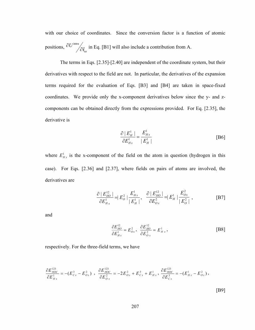
207

with our choice of coordinates. Since the conversion factor is a function of atomic

positions, αi

intra

rr∂

∂U in Eq. [B1] will also include a contribution from A.

The terms in Eqs. [2.35]-[2.40] are independent of the coordinate system, but their

derivatives with respect to the field are not. In particular, the derivatives of the expansion

terms required for the evaluation of Eqs. [B3] and [B4] are taken in space-fixed

coordinates. We provide only the x-component derivatives below since the y- and z-

components can be obtained directly from the expressions provided. For Eq. [2.35], the

derivative is

||||

1

1

1

1

H

xH

xH

H

EE

EE

=∂∂

[B6]

where 1xHE is the x-component of the field on the atom in question (hydrogen in this

case). For Eqs. [2.36] and [2.37], where fields on pairs of atoms are involved, the

derivatives are

||||

||1

12

1

12

H

xHO

xH

HO

EE

EEE

=∂∂

, ||

||||

2

21

2

12

O

xOH

xO

HO

EE

EEE

=∂∂

, [B7]

and

21

12

xOxH

HO EEE

=∂∂ , 1

2

12

xHxO

HO EEE

=∂∂ , [B8]

respectively. For the three-field terms, we have

)( 231

123

xOxCxH

HOC EEEE

−−=∂∂ , 132

2

123

2 xHxCxOxO

HOC EEEEE

++−=∂∂ , )( 21

3

123

xOxHxC

HOC EEE

E−−=

∂∂ ,

[B9]

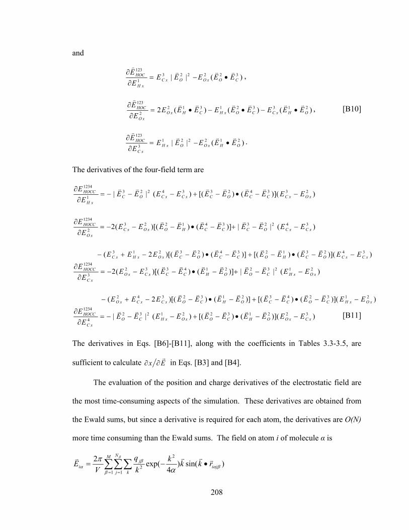
208

and

)(|| 3222231

123

COxOOxCxH

HOC EEEEEEE vvv)

•−=∂∂ ,

)()()(2 2133213122

123

OHxCCOxHCHxOxO

HOC EEEEEEEEEE

E vvvvvv)

•−•−•=∂∂ , [B10]

)(|| 2122213

123

OHxOOxHxC

HOC EEEEEE

E vvv)

•−=∂∂ .

The derivatives of the four-field term are

))](()[()(|| 233423342231

1234

xOxCCCOCxCxCOCxH

HOCC EEEEEEEEEEE

E−−•−+−−−=

∂∂ vvvvvv

)(||)]())[((2 342233412232

1234

xCxCOCCCHOxOxCxO

HOCC EEEEEEEEEEE

E−−+−•−−−=

∂∂ vvvvvv

))](()[()]())[(2( 3423123423213xCxCOCHOCCOCxOxHxC EEEEEEEEEEEEE −−•−+−•−−+−

vvvvvvvv

)(||)]())[((2 212322143323

1234

xOxHCOOHCCxCxOxC

HOCC EEEEEEEEEEE

E−−+−•−−−=

∂∂ vvvvvv

))](()[()]())[(2( 2132432132342xOxHCOCCOHCOxCxCxO EEEEEEEEEEEEE −−•−+−•−−+−

vvvvvvvv

))](()[()(|| 322132212324

1234

xCxOOHCOxOxHCOxC

HOCC EEEEEEEEEEE

E−−•−+−−−=

∂∂ vvvvvv [B11]

The derivatives in Eqs. [B6]-[B11], along with the coefficients in Tables 3.3-3.5, are

sufficient to calculate Exr

∂∂ in Eqs. [B3] and [B4].

The evaluation of the position and charge derivatives of the electrostatic field are

the most time-consuming aspects of the simulation. These derivatives are obtained from

the Ewald sums, but since a derivative is required for each atom, the derivatives are O(N)

more time consuming than the Ewald sums. The field on atom i of molecule α is

∑∑∑= =

•−=M N

j kji

ji rkkk

kq

VE

1 1

2

2 )sin()4

exp(2β

βαβ

α

β

απ vvvv

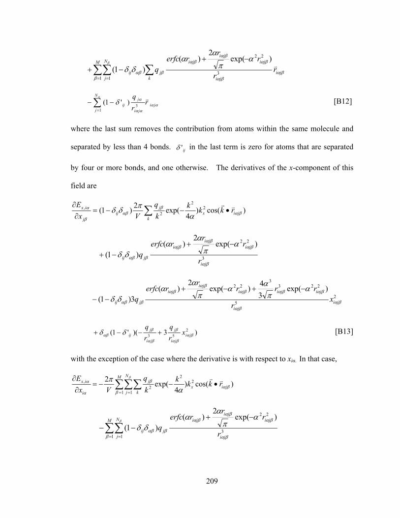
209

∑∑ ∑= =

−+−+

M N

j kji

ji

jiji

ji

jij rr

rr

rerfcq

1 13

22 )exp(2

)()1(

ββα

βα

βαβα

βα

βαβ

βα

πα

αδδ v

∑=

−−α

αααα

αδN

jji

ji

jij r

rq

13)'1( v [B12]

where the last sum removes the contribution from atoms within the same molecule and

separated by less than 4 bonds. ij'δ in the last term is zero for atoms that are separated

by four or more bonds, and one otherwise. The derivatives of the x-component of this

field are

∑ •−−=∂∂

kjix

jij

j

ix rkkkkq

VxE

)cos()4

exp(2)1( 22

2,

βαβ

αββ

α

απδδ vv

3

22 )exp(2

)()1(

βα

βαβα

βα

βαβ

απ

αα

δδji

jiji

ji

jij r

rr

rerfcq

−+−+

25

2233

22 )exp(34)exp(

2)(

3)1( βαβα

βαβαβαβα

βα

βαβ

απαα

πα

αδδ ji

ji

jijijiji

ji

jij xr

rrrr

rerfcq

−+−+−−

)3)('1( 253 βαβα

β

βα

βαβ δδ ji

ji

j

ji

jij x

rq

rq

+−−+ [B13]

with the exception of the case where the derivative is with respect to xiα. In that case,

∑∑∑= =

•−−=∂∂ M N

j kjix

j

i

ix rkkkkq

VxE

1 1

22

2, )cos()

4exp(2

ββα

β

α

αβ

απ vv

∑∑= =

−+−−

M N

j ji

jiji

ji

jij r

rr

rerfcq

1 13

22 )exp(2

)()1(

β βα

βαβα

βα

βαβ

βα

πα

αδδ

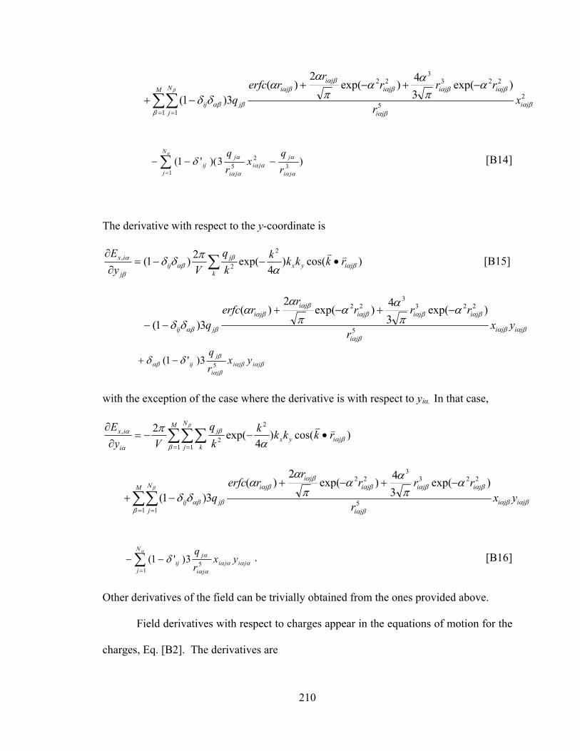
210

∑∑= =

−+−+−+

M N

jji

ji

jijijiji

ji

jij xr

rrrr

rerfcq

1 1

25

2233

22 )exp(34)exp(

2)(

3)1(β

βαβα

βαβαβαβα

βα

βαβ

βα

παα

πα

αδδ

)3)('1(1

32

5∑=

−−−α

αα

ααα

αα

αδN

j ji

jji

ji

jij r

qx

rq [B14]

The derivative with respect to the y-coordinate is

∑ •−−=∂∂

kjiyx

jij

j

ix rkkkkkq

VyE

)cos()4

exp(2)1(2

2,

βαβ

αββ

α

απδδ vv

[B15]

βαβαβα

βαβαβαβα

βα

βαβ

απαα

πα

αδδ jiji

ji

jijijiji

ji

jij yxr

rrrr

rerfcq 5

2233

22 )exp(34)exp(

2)(

3)1(−+−+

−−

βαβαβα

βαβ δδ jiji

ji

jij yx

rq

53)'1( −+

with the exception of the case where the derivative is with respect to yiα. In that case,

∑∑∑= =

•−−=∂∂ M N

j kjiyx

j

i

ix rkkkkkq

VyE

1 1

2

2, )cos()

4exp(2

ββα

β

α

αβ

απ vv

∑∑= =

−+−+−+

M N

jjiji

ji

jijijiji

ji

jij yxr

rrrr

rerfcq

1 15

2233

22 )exp(34)exp(

2)(

3)1(β

βαβαβα

βαβαβαβα

βα

βαβ

βα

παα

πα

αδδ

∑=

−−α

αααααα

αδN

jjiji

ji

jij yx

rq

153)'1( . [B16]

Other derivatives of the field can be trivially obtained from the ones provided above.

Field derivatives with respect to charges appear in the equations of motion for the

charges, Eq. [B2]. The derivatives are

211

∑ •−=∂∂

kji

j

i rkkkkVQ

E )sin()4

exp(12 2

2 βαβ

α

απ vvv

v

βαβα

βαβα

βα

αβ

απ

αα

δδ jiji

jiji

ji

ij rr

rr

rerfcv

3

22 )exp(2

)()1(

−+−+

βαβα

αβ δδ jiji

ij rr

v3

1)'1( −− [B17]

when jβ≠iα. The derivative vanishes when jβ=iα. That is,

0=∂∂

α

α

i

i

QEv

. [B18]

212

APPENDIX C Details of the potentials for 2-propanol

Semi-flexible models for 2-propanol developed in this work are described herein.

Models for other solvents and the selectors can be found elsewhere[112, 161, 181].

The intramolecular potential, which dictates the energetic costs for changes in

molecular conformations, consists of four parts: bond stretching, angle bending, dihedral

torsion, and improper torsion. These potentials are listed in Eqs. [2.7]-[2.10]. In this work,

all bonds of 2-propanol are kept fixed using the Rattle algorithm[83] during the

simulations, and 19 bends and 3 torsions are employed to represent the molecular

flexibility. The equilibrium bond angles are obtained from the global energy minimum

and bending potentials are obtained by least squares fits of Eq. [2.8] to nine energy

calculations, where the angle is varied within sixteen degrees of the equilibrium value. As

shown in Eq. [2.9], the torsions are represented by modified Ryckaert-Bellemans[189]

potentials. Each torsional potential is extracted from 36 B3LYP/aug-cc-pVDZ

calculations as the angle is varied from zero to 360 degrees, in steps of 10 degrees.

Initial atomic positions and CHELPG charges[110] are extracted from B3LYP/aug-

cc-pVDZ global energy minimum. For the nonbonding potential parameters, the

CHARMM parameters for Lennard-Jones (LJ) potential and CHELPG charges from the

ab initio global minimum are applied.

213

The parameterization of the fluctuating charge model has been discussed in detail

in Chapter 3. Briefly, the molecule was placed in 30 diverse fields and atomic charges

were evaluated by the CHELPG algorithm applied to B3LYP/aug-cc-pVDZ calculations.

Based on the fitting of the molecular response, the 0~iχ and 0

iiJ parameters were extracted.

Similar to the findings for ethanol in Chapter 3, the atomic electronegativities derived

specifically for 2-propanol were larger than the transferrable CHARMM-FC values[53]

for most atoms. All electronic structure calculations are performed using the Gaussian 03

program[135].

LJ and FC parameters

Atom

No. Atom σ(Å)

ε

(kJ/mol)

CHARMM 0iiJ

(kcal/mol.|e|2)

0iiJ (this

work)

(kcal/mol.|e|2)

CHARMM oiχ~

(kcal/mol.|e|)

Shifted oiχ~

(kcal/mol.|e|)

oiχ~ (this

work)

(kcal/mol.|e|)

0iQ

(|e|)

1 O 0.312 0.7113 307.20 317.07 364.85 101.66 107.41 -0.685

2 H 0.05 0.1000 517.26 544.06 263.19 0.00 0.00 0.369

3 C 0.35 0.2761 196.88 212.95 306.79 43.60 71.68 0.591

4 H 0.25 0.1255 501.42 470.07 319.83 56.64 66.18 -0.084

5 C 0.35 0.2761 240.34 283.89 319.65 56.46 66.16 -0.298

6 C 0.35 0.2761 240.34 283.89 319.65 56.46 66.16 -0.298

7 H 0.25 0.1255 501.42 576.59 315.56 52.37 50.94 0.067

8 H 0.25 0.1255 501.42 576.59 315.56 52.37 50.94 0.067

9 H 0.25 0.1255 501.42 576.59 315.56 52.37 50.94 0.067

10 H 0.25 0.1255 501.42 576.59 315.56 52.37 50.94 0.067

11 H 0.25 0.1255 501.42 576.59 315.56 52.37 50.94 0.067

12 H 0.25 0.1255 501.42 576.59 315.56 52.37 50.94 0.067

214

Angle bending

Angle θ(deg) kθ(kJ. mol-1 . deg-2)

3,1,2 108.81 0.065813

4,3,1 108.80 0.090213

5,3,1 108.72 0.121507

6,3,1 108.72 0.121507

5,3,4 108.81 0.077831

6,3,4 108.81 0.077831

6,3,5 112.87 0.107790

7,5,3 110.56 0.066107

8,5,3 110.56 0.066107

9,5,3 110.56 0.066107

8,5,7 108.36 0.060220

9,5,7 108.36 0.060220

9,5,8 108.36 0.060220

10,6,3 110.56 0.066107

11,6,3 110.56 0.066107

12,6,3 110.56 0.066107

11,6,10 108.36 0.060220

12,6,10 108.36 0.060220

12,6,11 108.36 0.060220

Torsions

Torsion c0, c1, c2, c3, c4, c5, c6 (kJ/mol)

2,1,3,4 7.76,1.89,6.06,10.76,-4.56,-0.94,2.44

1,3,5,7 6.66,-20.53,2.04,28.26,-7.61,-0.96,5.68

1,3,6,10 6.66,-20.53,2.04,28.26,-7.61,-0.96,5.68