Embed Size (px)
Citation preview
1
Version of 19/05/2015
The Intergenerational Transmission of BMI in China
Peter Dolton
(University of Sussex)
(Centre for Economic Performance
London School of Economics)
and
Mimi Xiao (University of Sussex)
Abstract
Based on the CHNS longitudinal data from 1989 to 2009 and using BMI z-score as the measure
of adiposity, we estimate the intergenerational transmission of BMI in China. The OLS
estimates suggest that a one standard deviation increase in father’s BMI is associated with an
increase of 20% in child’s BMI z-score. The corresponding figure is around 22% for the
transmission between mother and child’s BMI z-score. These estimates decrease to 14% for
father-child and 12% for mother-child when we control for family fixed effects. We also find
this intergenerational correlation tends to be higher among children of higher BMI levels,
though this tendency becomes weaker as children approach adulthood (i.e. aged 16-18 years
old).
Key words: intergenerational; adiposity; China
Address for Correspondence:
Prof Peter Dolton
Department of Economics
University of Sussex,
Brighton
BN1 9SL
Email: [email protected]
JEL reference numbers: I15
2
1. Introduction
What role does intergenerational transmission, due to processes inside the family, play in
the determination of health and economic outcomes of young people? This question is
particularly interesting in a developing country like China that is in the throes of a nutritional
and epidemiological transformation. China has experienced huge changes in rural to urban
migration with massive urbanisation (van de Poel et al 2009, Song 2013) and undergone an
attendant radical restructuring of its labour market (Knight and Song 2012). In rural China, the
average nominal income in 2011 (6,194 yuan) is nearly ten times what it was in 1990 (686
yuan); in urban China, the average nominal income increased even more dramatically, from
1,510 yuan in 1990 to 19,118 yuan in 20111. Since 1978, the resultant significant improvement
of Chinese living standards has been sustained and accelerated over recent decades (Klein and
Ozmucur 2002, Tafreschi 2014).
With the transformation of the Chinese economy, more calorific and higher quality food
has become available, leading to a shift in dietary habits and an improvement in nutritional
intake and energy composition (Du et al. 2002). The proportion of rice and wheat in the average
diet has decreased, whilst the share of pork has increased (Guo et al. 2000). More energy is
now consumed from fat, with an increasing consumption of energy-dense foods (Popkin 2001).
Over the same period, the level of physical activity (such as cycling and walking) has been
falling due to the rapid motorization (Bell et al. 2012). As a result, the health outcomes of the
Chinese population have undergone a dramatic transformation in the past 25 years. Evidence
from the China Health and Nutrition Survey (CHNS) (Popkin et al 2010) data (which is used
in this study) shows that there is an increase in the average Body Mass Index (BMI).
Particularly, there has been a rightward shift in the whole distribution of BMI over the period
from 1989 to 1997, with the proportion who are underweight declining, and the proportion who
are obese increasing. This observation is particularly pronounced amongst children and
adolescents. For adults aged between 39 and 59, the fraction of those who are underweight has
decreased from 14.5% to 13.1%, and the overweight has increased from 6.4% to 7.7% (Popkin
2008). China, which used to have one of the leanest populations in the world, now has over
one fifth of all the one billion obese people in the world (Wu 2006). In addition, with the rising
income inequality (where the Gini coefficient is high at 0.61), there are also substantial health
1 These statistics are from National Bureau of Statistics of China, 2012.
3
inequalities across regions (Morgan 2000). Given the intergenerational income correlation
estimate of 0.6 in China (Gong 2012), the estimation of the intergenerational BMI correlation
(IBC)2 will provide some insight into the investigation of intergenerational mobility and the
prevailing level of social mobility in China.
There is a relatively small variability in the magnitude of intergenerational BMI
relationship across countries (Dolton and Xiao 2015), and this relationship tends to be stronger
at the fatter end of child’s BMI distribution. Taking advantage of the excellent CHNS panel
data we study China in detail and use BMI z-score of both parents and children over time to
conduct a more comprehensive analysis of the intergenerational process of adiposity
transmission. In addition to estimates of the IBC at the conditional mean and across the
distribution, this study makes two distinct contributions to the literature.
First, in addition to the mother only and child or father only and child3 transmission which
is sometimes explored in the literature, we examine the BMI effects of both father and mother.
In other words, both father and mother’s BMI measure are included into the transmission
regression. This helps us to explore the genetic and environmental effects that both parents
exert on children. We argue that we explore the variation of intra-household mechanism by
controlling for both the father and mother’s BMI measure rather than merely using either the
father or the mother. Empirically, since the CHNS data is a longitudinal dataset which records
data on the same individuals repeatedly over time, then this panel structure allows us to explore
the dynamic pattern of change in children’s adiposity outcomes as they age. We start by
conditioning on their own BMI z-score in a previous time period. In addition, we net out for
unobserved intra-household heterogeneity by controlling for family fixed effects. This
facilitates the estimation of the mechanism whereby the change in children’s adiposity outcome
is considered as a function of the change in parents’ adiposity outcome. This is different from
most of the previous studies which mainly use levels of BMI in a cross section, taking no
account of the potential endogeneity of child and parental BMI through the correlation of these
measures with unobserved heterogeneity.
2 From this point on we will distinguish between the intergenerational BMI correlation (IBC) and the
intergenerational BMI elasticity (IBE). The IBC is derived from the regression which is estimated in raw BMI
or BMI z scores (these models are equivalent in terms of the interpretation of the coefficient). The IBE is
derived from a model in which the double log transformation is used and child’s BMI is regressed on parents
BMI. Appendix B makes this distinction and its advantages and disadvantages clear. 3 In an earlier version of this paper we explored the possibility of an interactive assortative mating (Kalmijn,
1994, Mare 1991) component to this relationship. We found only scant evidence of this. Details are available
from the authors on request.
4
Second, we also more fully explore the observed heterogeneity of this intergenerational
adiposity transmission process. We do this in several ways. We examine how the IBC varies
as the child grows older. We find that this relationship tends to grow during the first half part
of childhood4, and then declines in adolescence until adulthood. We also separately analyse the
subsample of children aged between 16 and 18 years old, based on the argument that the
anthropometric measurement of children within this age range is most similar to that of adults
and it is this relationship of adult child outcomes with their parents which is of most interest to
a study of the social mobility process. We also examine whether the IBC changes with different
levels of parental socioeconomic status – i.e. whether there is a ‘social gradient’ to
intergeneration adiposity transmission. We do not find a substantial variability in the magnitude
of intergenerational correlation of BMI with respect to different levels of family socioeconomic
factors. Finally, we apply quantile estimation to examine the heterogeneity of the
intergenerational adiposity relationship. We find that this correlation is around 0.31 per parent
for the lowest child’s BMI and around 0.18 at the highest child’s BMI – which demonstrates
the considerable difference in the IBC across the BMI distribution of children.
4 The father-child correlation of BMI z-score increases when the child’s aged from 0 to 10 years old, whereas
the mother-child IBE increases until the child’s ages reached around 12 years old.
5
2. The Intergenerational Transmission of Health Attributes
The study of intergenerational transmission processes began with Francis Galton (1869)
who examined the first detailed data on offspring’s height and their parents’ height. He argued
that an individual’s characteristics are correlated with those of their parents and at the same
time “regress to mediocrity”. More specifically, the individual characteristics (such as height
and weight) are closer to the population mean than those of their parents. This finding was the
basis of Becker-Tomes model (1986) of intergenerational human capital transmission which
has been extended by others (Goldberger 1989, Han and Mulligan 2001, Mulligan 1999, Black
et al 2005) and used as the starting point in the analysis of intergenerational transmission of
health (Ahlburg 1998, Doyle et al 2009) and intergenerational mobility through education (for
example Anger and Heineck 2010), or income (see for example, Bjorklund and Jantti 2009,
Dearden et al 1997). This has also led to a growing literature on the effect of obesity on other
outcomes (e.g. Scholder et al 2012).
There is now a growing economics literature on the intergenerational transmission of
various health outcomes, such as: Health status (Akbulut and Kugler 2007), birth weight
(Emanuel et al 1992, Conley and Bennett 2000, Currie and Moretti 2005, Royer 2013), self-
rated health (Coneus and Spiess 2012, Thompson 2012), longevity (Trannoy et al. 2010),
smoking behaviour (Loureiro et al. 2006) and height and weight (Eriksson et al 2014). These
studies find significant positive correlations across generations. In terms of adiposity and
related measures, a large proportion of the studies are published in the medical, biological or
epidemiological journals, they show parental health outcomes are consistently correlated with
children’s outcomes. (See Moll et al (1991), who find an IBC of .22, Heller et al (1984) who
find and IBC of .23, Perusse et al (1988) who find an IBC of .20, Tambs et al (1991) who find
an IBC of .20 and Li et al (2009) who get IBC estimates between .17-.33 for mothers with their
children at different ages and .15-.36 for fathers with their children at different ages) . A
summary of this literature is provided by Boucher and Perusse (1994). These papers tend to
focus on either raw, simple unconditional correlations or with very limited controls. Another
strand of the literature exclusively examines data on twins and adoptees with the expressed
intention of separately identifying the genetic or environmental component of obesity
transmission (see Maes et al 1997, and Dubois et al 2012). Other papers examine only the
tendency to obesity (as a limited binary outcome) between generations and not the IBE or ICC
(Martin 2008).

6
A significant departure from the epidemiological literature this was first provided by
Classen (2010). Using data from the National Longitudinal Survey of Youth 1979 (NLSY 1979)
and the Young Adults of the NLSY79, he estimates the intergenerational transmission of BMI
between children and their mother when both generations are between the age of 16 and 24, he
runs the regression which includes only mother and finds the intergenerational elasticity is
significant and around 0.35. He finds this elasticity varies by gender with a stronger correlation
between mothers and daughters, compared to that between mothers and sons. Additionally,
Classen (2010) estimates the intergenerational BMI relationship across the distribution of
child’s BMI by applying quantile estimation. His results indicate that the intergenerational BMI
relationship tends to be stronger among children with higher levels of BMI, and he argues that
the strong persistence of obesity may also provide an insight into the more general nature of
the intergenerational transmission.
In the context of developing countries, using the China Health and Nutrition longitudinal
Survey (CHNS) (1989-2009), Eriksson, Pan, and Qin (2014) estimate the intergenerational
transmission of health status, using height z-score and weight z-score as the health measure.
They find a strong correlation between parents’ health and their children’s health after
accounting for various parental socioeconomic factors (education and type of occupation),
household characteristics (whether the household has a flush toilet) and the health-care factors
(the distance to the nearest health centre in the community). Specifically they find a correlation
of ..23 -.27 of each parent with a child’s weight. To correct for the unobserved heterogeneity,
they use the age and gender adjusted average parents’ BMI in parents’ province as the
instrument for parental BMI variable. Additionally, using the decomposition analysis, they find
the urban-rural differential in parental health explains 15-27% of urban-rural disparity in
child’s health, in addition to the urban-rural differential in parental education and income,
which plays a major role.
The second concern of this paper is the observed heterogeneity of the adiposity - in terms
of the variability of the intergenerational transmission of BMI with respect to different family
socioeconomic factors (see Laitenen et al 2001) but evidence is lacking. Some studies have
suggested the intergenerational correlation of health outcomes tends to be stronger at lower
levels of SES in both developed countries and developed countries. Based on a dataset on
California births from 1960s to around 2005, Currie and Moretti (2005) find that children of
low birth weight mothers are around 50% more likely to have low birth weight babies, and

7
maternal poverty is strongly correlated with low birth weight of child, they argue that this
intergenerational transmission of low birth weight is associated with the intergenerational
transmission of low income (i.e. poverty cycle), since parent’s income affects child’s health,
and child’s health affects their future education and earnings. Using the US data, Thompson
(2013) also finds that the intergenerational transmission of health is stronger among families
of low SES. In the setting of developing countries, based on individual survey data on 2.24
million children born to 600,000 mothers over the period from 1970 to 2000 in 38 developing
countries, Bhalotra and Rawlings (2013) find children of shorter mothers or mothers with
poorer health at birth are more sensitive to changes in the socioeconomic environment, and
their survival rate is lower. We examine the intergenerational transmission of adiposity with
respect to income, education and occupation of the parents as well as across the age of the child
and with respect to the distribution of child BMI.
8
3. Data and Method
3.1 Data
The longitudinal data used in this study comes from eight waves (1989, 1991, 1993, 1997,
2000, 2004, 2006, and 2009) of the China Health and Nutrition Survey (CHNS)5. CHNS is
conducted as a joint project of the Carolina Population Center at the University of North
Carolina at Chapel Hill and China’s National Institute for Nutrition and Food Safety and the
China Center for Disease Control and Prevention. It covers urban and rural areas in nine
provinces that vary substantially in geology, economic development and public resources. The
data contains health outcomes, demographic and anthropometric measurements for members
of the sampled households, including medically measured heights and weights. It also includes
information on social and economic indicators such as education, household income and labor
market outcomes such as occupations. The CHNS sample is not strictly representative of the
whole of China but is designed to be randomly selected from households in eight provinces6--
- Liaoning, Shandong, Henan, Jiangsu, Hubei, Hunan, Guizhou and Guangxi. The CHNS
employs a multistage, random cluster process to draw the sample in each of the provinces7. Our
sample is restricted to children under 18 years old with anthropometric information on both the
biological father and mother. We chose age 18 as the threshold since this is the age used to
distinguish between adult and child in the CHNS physical examination dataset (where the
anthropometric information is included). Additionally, children within this age range normally
live with their parents and rely on their parents for nutritional intake and health care. As a
result, this sample includes 14,077 child-parent-wave observations made up by 6,044 children
with their fathers and mothers.
A very important feature of the CHNS is that the height and weight in our data are
measured medically rather than self-assessed. Such data is rarely available in other longitudinal
data. Self-assessed anthropometric measures tend to be biased, among which weight and BMI
tend to be under-reported whereas height tends to be over-reported (Gorber et al. 2009), this
5 The CHNS is publicly available at http://www.cpc.unc.edu/projects/china 6 In 1997 Liaoning was not able to participate and a new province-Hei Longjiang was added as a replacement,
then Liaoning returned to the survey in 2000. 7 See Popkin et al. (2010) for a detailed introduction on the CHNS survey.

9
may lead to an underestimation of BMI when it is based on the self-assessed data rather than
the medically measured data8. Therefore, the fact that the height and weight in the CHNS data
were recorded by the trained medical staff may help to improve the accuracy of our estimates
of intergenerational correlation of BMI (Spencer et al. 2002).
We use BMI z-score rather than raw BMI, since BMI z-score reflects the relative position
to the normed reference population (the sample from WHO macro software) which adjusts for
age and gender 9 . The conversion of z-score can be made using the 2006 WHO Growth
Standards for preschool children and the 2007 WHO Growth Reference for school age children
and adolescents. In Stata, this conversion is implemented using a program from the WHO
website10.
3.2 Descriptive Statistics
This section presents some descriptive statistics of our sample. Since BMI z-score is
adjusted for age and gender, this feature facilitates the comparison of adiposity distribution
across groups of different age levels, in our case this is particularly true when we plot the
distribution of adult parents’ and child’s adiposity distribution together, as we show in Figure
3.2 and Figure 3.3. In terms of the classification, we follow the WHO growth
reference/standard (Wang and Chen, 2012) and use the following classification: underweight
if BMI z-score <-1.04; normal if -1.04<=BMI z-score<1.04; overweight if 1.04<=BMI z-
score<1.64; obese if BMI z-score>=1.64. This classification applies to both adults and children
since the WHO transformed BMI z-score accounts for both age and gender.
Figure 1 suggests the density of child’s BMI z-score for cohorts aged less than six, seven
to twelve and thirteen to eighteen. The left-ward shift of child’s BMI z-score across three age
cohorts indicates that the distribution of the BMI shifts upwards as their age increases. This is
because that the child’s BMI values in our sample tend to be lower than the reference
population in the ‘Anthro’ software. Specifically, the average BMI of Asian population tends
8 See Spencer et al (2002) and Sherry et al (2007). 9 See Appendix B for a description of BMI z-score and a discussion on BMI z-score and BMI. We also
conducted the analysis using raw BMI values. The corresponding results are available on request from the
authors. They are consistent with the results using BMI z-score here. 10 They can be downloaded from http://www.who.int/childgrowth/software/en/ for Child growth standards (0~5
years old) and http://www.who.int/growthref/tools/en/ for Growth reference (5~19 years old).

10
to be lower than that of non-Asian population (WHO 2004). This decline is relative to the
external (world) reference population rather than the internal (our CHNS sample) reference
population, and the left-wards shift of child’s BMI density does not imply a decrease in the
child’s true BMI values as their age increase. When it comes to the intergenerational
relationship of BMI z-score, Figure 2 and Figure 3 suggest (respectively) that the distribution
of child’s BMI z-score shifts towards the left relative to their father and mother. This trend
indicates a shift towards lower BMI z-score among children relative to their parents. This effect
is found mainly because of the use of the WHO referencing of the BMI z-score. The reverse
case is found by Classen (2010) using NLSY79 data in the United States, he shows a shift
towards higher BMI levels among children relative to their mother.
There are three factors that explain these patterns. First, Figure 1 shows that when we
consider much recent cohorts of children, they are getting fatter, in the sense that the proportion
of young children aged below six, who are obese is greater than the share of older children who
are obese. Second, although the children’s distribution, relative to their mother and father is
shifting leftwards (due to the bias in the WHO reference group), it is the case that the fraction
of children who are obese is larger than the fraction of fathers (Figure 2) or mothers who are
obese (Figure 3). Third, the fraction of fathers and mothers who are obese is increasing over
time. To see this, we clustered observations by survey period (1989, 1991 and 1993, 1997 and
2001, 2004, 2006 and 2009) and find that the fractions of fathers and mothers who are obese
have shifted to the right over time. Likewise, for children within the same age range (<=6, 7-
12, and 13-18), the fraction of obesity is also increasing over time11.
11 These figures are presented in Appendix A, Figure A4.

11
Figure 1: Distribution of child's BMI z-score by age group
(Using WHO Age and Gender Adjustment)
Source: own calculation
Figure 2: Distribution of father and child's BMI z-score
(Using WHO Age and Gender Adjustment)
Source: own calculation
Underweight
Overw
eig
ht Obese
Normal
0.1
.2.3
.4
Den
sity
-5 0 5BMI-for-age z-score
Child's kernel density <=6 years old
Child's kernel density 7~12 years old
Child's kernel density 13~18 years old
kernel = epanechnikov, bandwidth = 0.2082
Kernel density estimate
Underweight
Overw
eig
ht
ObeseNormal
0
.1
.2
.3
.4
Den
sity
-5 0 5BMI-for-age z-score
Child's kernel density
Father's kernel density
kernel = epanechnikov, bandwidth = 0.1453
Density of BMI Father&Child

12
Figure 3: Distribution of mother and child's BMI z-score
(Using WHO Age and Gender Adjustment)
Source: own calculation
Figure 4: Distribution of father, mother and child’s BMI z-score
(Using WHO Age and Gender Adjustment)
Source: own calculation
Underweight
Overw
eig
ht
Obese
Normal
0
.1
.2
.3
.4
.5
Den
sity
-5 0 5BMI-for-age z-score
Child's kernel density
Mother's kernel density
kernel = epanechnikov, bandwidth = 0.1453
Density of BMI Mother&Child
underweight
Overw
eig
ht
ObeseNormal
0.1
.2.3
.4.5
-5 0 5BMI-for-age z-score
Child's kernel density Father's kernel density
Mother's kernel density
Density of BMI father-mother-child
13
4 Empirical Model
The empirical estimating equation we employ is as follows:
𝑦𝑖 = 𝛿 + 𝛼y𝑓𝑖 + 𝛽y𝑚𝑖 + 𝛾𝑥𝑝 + 𝜃𝑔𝑖 + 휀𝑖 (1)
where 𝑖 indexes individual child observations and 휀𝑖 captures the transmitted stochastic error
term. In the equation, child’s health outcome 𝑦𝑖 is a function of child 𝑖 ’s father’s health
outcome, 𝑦𝑓𝑖, and mother’s health outcome, 𝑦𝑚𝑖, 𝑥𝑝 denotes the age variables of father and
mother and other controls, and 𝑔𝑖 captures child 𝑖 ’s age annual dummies, gender and the
interaction term between them. Notice here we use age annual dummies rather than the
continuous variable of BMI to account for the potential non-linear relationship between age
and BMI z-score. Equation (1) is the baseline equation we use in this study. We are principally
interested in the 𝛼 and 𝛽 coefficients which parameterize the IBC between the child and the
father and mother respectively.
In addition to the pooled OLS estimation, based on the longitudinal structure of the CHNS
data, we also investigate the simplest dynamic pattern of child’s BMI measure, equation (1) is
estimated with the incorporation of lagged child’s BMI z-score, yi,t−1, in doing so we wish to
net out for the individual unobserved heterogeneity .
𝑦𝑖𝑡 = δ + 𝛼y𝑓𝑡 + 𝛽y𝑚𝑡 + 𝛾𝑦𝑖,𝑡−1 + 휀𝑖𝑡 (2)
Where 𝑡 denote observations referenced to a specific time period (or wave of the data).
The IBC measures the extent to which (i) biological/genetic factors and (ii) a shared
family environment contribute to the intergenerational transmission of BMI from parents to
their offspring. It does not tell us much about the mechanism in terms of how much is
specifically attributable to genetic factors and how much of this correlation is specifically due
to environmental factors. The longitudinal structure of CHNS data allows us to condition out
unobserved genetic effects and that part of the unobserved environmental effects which are not
changing over time. This logic suggests that the fixed effects estimates mainly capture the
effects of changes in shared environmental factors over time.

14
Since both child’s health and parents’ health are affected by time-invariant unobserved
individual heterogeneity, 𝑓𝑖, such as eating habits, health behavior and genetic components.
The panel structure of the data allows us to estimate equation (1) in an individual fixed effect
framework. This can be written in the form of equation (3) below which takes into account an
individual fixed effect 𝑓𝑖.
𝑦𝑖𝑡 = δ + 𝛼𝑦𝑓𝑖𝑡 + 𝛽y𝑚𝑖𝑡 + 𝛾𝑥𝑝𝑡 + 𝑓𝑖 + 휀𝑖𝑡 (3)
However, it is also reasonable to assume that unobserved family environmental factors
remain constant. For instance, the family routine, such as eating and sleeping time shared
among household members, normally do not change much over time. More importantly, the
pattern of food allocation among household members normally remains relatively constant.
These patterns, together with, who is in control of the family income (Thomas 1990), who takes
a larger share of energy-intensive activities (Pitt et al. 1990), whether the parents have a
preference for sons (Qian 2008) or lower-birth-order children (Dasgupta 1993), can all affect
both parental and children’s BMI outcomes. Thus, household fixed effects are applied to
estimate equation (1), i.e., fixed effects model is estimated using the following equation (4).
y𝑖𝑗𝑡 = δ + 𝛼y𝑓𝑖𝑗𝑡 + 𝛽y𝑚𝑖𝑗𝑡 + 𝛾𝑥𝑝𝑗𝑡 + ℎ𝑗 + 휀𝑖𝑡 (4)
Where 𝑗 indexes household/family observations. In household 𝑗, child 𝑖’s health is a function
of father’s health, 𝑦𝑓𝑗𝑡, and mother’s health, 𝑦𝑚𝑗𝑡 , ℎ𝑗 denotes the household family fixed
effects. This equation can only be identified when we have data on more than one sibling inside
the family - for which, by assumption, the ℎ𝑗 term is the same. We can estimate this model on
the data as in a subset of this data there are more than one child in each household. In all of the
estimation which follows our interest is on the 𝛼 and 𝛽 coefficients which respectively
measure the relationship of BMI z-score for father-child and mother-child. The biological laws
of nature suggest that both coefficients will be positive. What is at issue here is how large they
are, compared with the OLS estimates from equation (1).
In addition, we estimate equation (1) with respect to different levels of family social
economic status, measured by family income, mother’s education, father’s occupation and the
time duration when the family was in poverty, respectively; we estimate the IBC across

15
different quantiles of child’s BMI. We also estimate the intergenerational correlation of BMI
z-score by age group, and conduct quantile estimation on samples aged 16~18 years old to
examine the probability that this relationship is structurally different when the children become
adults.
5 Empirical Results
5.1 Ordinary Least Squares (OLS)
Before presenting the results, it is necessary to clarify that the intergenerational
relationship of BMI z-score cannot be used to isolate the genetic effects from the environmental
effects 12 . Instead, it explores the role of common genes and environment in the
intergenerational transmission of anthropometric tendency (Gruber 2009).
Table 1 presents the baseline pooled OLS estimates (with around 14,000 observations) in
single-parent and both-parents version of equation (1). Column (1) shows the correlation
between father’s BMI z-score and child’s BMI z-score when the regression only controls for
father’s BMI z-score, the coefficient of 0.223 suggests that one standard deviation increase in
father’s BMI z-score is associated with an increase of 0.223 in child’s BMI z-score. Similarly,
column (2) suggests that the association between mother and child’s BMI z-score in the sample
is 0.208. The coefficients for child’s age dummies are mostly negative, column (3) suggests
that this intergenerational correlation appears stronger after we control for child’s age and the
interaction of child’s age with their gender13. This indicates that Chinese children’s BMI z-
scores decline with age, relative to the WHO reference group. This corresponds to our finding
in Figure 1.
The results imply a marginally greater role for the environment and genes that a father and
child share together than the mother and child share together, in the intergenerational
transmission of BMI z-score. We have conducted t-tests to compare these two estimates in each
regression, the results suggest that the estimate coefficient on father’s BMI z-score is
12 Note that the intergenerational correlation of BMI z-score shares this property with the intergenerational
correlation of income and education which cannot distinguish between ‘inherited’ factors from family and
shared environment influences. 13 In results not reported we included an interaction term in mother and father BMI which was always
statistically insignificant.
16
significantly greater than that on mother’s BMI z-score. This result is robust when we control
for both father and mother’s BMI z-score, the magnitude of the coefficients on both the mother
and father fall slightly14. This result is counter to some studies in other countries, for example
Anderson (2012), which find a stronger influence of maternal health status (e.g. obesity) than
paternal health on child’s BMI. She attributes this relative importance of mother’s health to the
fact that mother is usually the primary caregiver in the family responsible for the diet and health
care of the child. However, some studies also find that this intergenerational correlation does
not differ substantially between the father and the mother, using 4,654 complete parent–
offspring trios in Avon Longitudinal Study of Parents and Children (ALSPAC), Smith et
al.(2007) find that the correlation between parental BMI and children’s BMI at age 7.5 was
similar for both parents.
Table 1: OLS estimates of the intergenerational correlation of BMI z-score.
(1) (2) (3) (4) (5) (6)
Dependent Variable: BMI z-score of child
BMI z-score of 0.223*** 0.244*** 0.237*** 0.198*** 0.181***
Father (0.0155) (0.0141) (0.0171) (0.0175) (0.0177)
BMI z-score of 0.208*** 0.235*** 0.221*** 0.191*** 0.160***
Mother (0.0174) (0.0166) (0.0200) (0.0195) (0.0216)
Lagged BMI 0.328***
z-score of child (0.0151)
Household
characteristics
Y Y Y
Year Dummies Y Y
Province Dummies Y Y
Province*Year
Interactions
Y Y
N 13,943 13,943 13,943 9,536 9,536 5,484
R-squared 0.027 0.021 0.189 0.193 0.224 0.298
Note: the regression (3)-(6) also include: age dummies of child, gender of child and the interactions between
them, father and mother’s age. Household characteristics include the category of household income per capita,
household size , the type of father’s occupation , the highest education degree mother attained. Standard errors
are clustered at the household level in parentheses, *** p<0.01, ** p<0.05, * p<0.1
Next we include household characteristics, regional dummies, year dummies and the
interactions between them in the equation - the results are presented in column (5). Column (1)
14 Compared with the results when the equation does not include father and mother’s BMI z-score, they are not
reported here.

17
suggests that after we control for household socioeconomic factors, which include: the category
of father’s occupation; the highest education degree of mother; the number of people in the
household and the category of household income per capita; then the estimates for father and
mother’s BMI effects decrease slightly compared with the baseline estimates (column (3) of
Table 1). Column (5) suggests there is a further appreciable decrease in the estimates for father
and mother’s BMI effects after we control for the fixed effects for child’s province of residence.
This is consistent with the previous studies that find that there is a substantial disparity in
child’s health status across regions in China. We also control for the time trend by including
the survey year dummies in the estimation; in column (5) we control for provincial-varying
time trends that may have occurred during the survey period used in this study. The results
suggest that the inclusion of potential environmental factors does not significantly reduce the
estimates of IBC, which is consistent with the prior studies (Thompson 2012).
In column (6) we turn to a basic (flexible) first difference model in which we control for
the child’s BMI z-score at a previous time period. 15 This reduces the sample to 7,918
observations. Here, the magnitude of these correlations understandably shrink slightly (to
around 0.17) when equation (1) includes the child’s lagged BMI z-score, where the coefficient
of this term is around 0.33 (column (6)). This result shows that the change of child’s BMI status
is strongly correlated with his/her BMI status in the previous year, i.e. there is a strong
persistence in child’s BMI over time.
5.2 Panel Fixed Effects (FE)
One of the really important features of the CHNS data is that it is longitudinal – this affords
us the possibility of estimation by panel fixed effects which means we can factor out elements
of unobserved heterogeneity which may confound the results we have so far reported. This
means using the longitudinal element of the data and model a child’s BMI z-score over the life
course of their childhood (or whatever part of it we observe) between 1989 and 2009. In doing
so we are able to - by turns - control for individual specific unobserved heterogeneity and
family specific unobserved heterogeneity. Our results are presented in the Table 2 and Table 3,
15 Nickell (1981) suggests that a ‘quasi-fixed effects estimate with a lagged dependent variable may downwardly
bias the coefficient of the lagged dependent variable. But this coefficient is not our central concern in this
study,.

18
respectively. Care needs to be taken in interpreting these results in comparison to Table 1. In
Table 1 we report simple correlations taking no account of the panel element of the data -
treating all observations occurring at any point in time as independent. In contrast, the panel
estimates specify the dynamic underlying intergenerational correlation of BMI z-score over the
childhood life course after having netted out for family and individual unobserved
heterogeneity.
The individual fixed effects estimates from equation (3) are provided in Table 2. This table
suggests that the intergenerational relationship of BMI z-score remains significant after the
regression controls for time-invariant unobserved individual characteristics. The individual
fixed effect estimates (0.151 and 0.160) are lower than the previous pooled OLS estimates
(0.244 and 0.235), this indicates a potential upward bias in the pooled OLS estimates due to
the omission of unobserved individual heterogeneity.

19
Table 2: Individual Fixed Effects Estimates of the intergenerational correlation of BMI
z-score.
(1) (2) (3)
Dependent Variable: BMI z-score of child
BMI z-score of father 0.151*** 0.151*** 0.138***
(0.0301) (0.0377) (0.0374)
BMI z-score of mother 0.160*** 0.135*** 0.118***
(0.0350) (0.0383) (0.0403)
Age dummies of child, gender of
child and the interactions between
them, father and mother’s age.
Y Y Y
Household characteristics Y Y
Individual Fixed Effects, Year
dummies, Province dummies,
Province*Year interactions
Y
Constant 3.533** 2.549 -5.511**
(1.482) (1.741) (2.752)
Observations 13,943 9,536 9,536
R-squared 0.159 0.154 0.186
Number of individuals 6,027 4,341 4,341
Standard errors are clustered at the household level in parentheses, *** p<0.01, ** p<0.05, * p<0.1
Table 3 presents family fixed effects estimates of the IBC. Looking at the magnitudes of
these estimates suggest that these family fixed effect estimates are very similar to the individual
fixed effect estimates. Compared with the OLS estimates, these fixed effects estimates provide
some information on the short-term environmental effects through differentiating out the
unobserved genetic effects and the long-term family and environmental effects which are
assumed invariant with time. In other words, the OLS estimates of the IBC provide a raw total
descriptive conditional correlation of this intergenerational correlation of the BMI. If we want
to say something on the mechanism- separating different channels of intergenerational
transmission - then the fixed effects estimates provide some evidence about the effects of
changes in environmental family factors (i.e. from year to year), such as change in the dietary
conditions and other factors which may have changed in the family like the type of transport
used. Hence the difference between the OLS and fixed effect estimates tell us something about
the factors which do not change in the family over time – which may be the family
environmental factors which remain constant but might well predominately be biological or
genetic factors which are likely to remain constant over time.

20
More specifically, the individual effect results indicate the effects of individual specific
parents on the individual specific child, and the household fixed effect results are more likely
to be associated with the difference between child 𝑖 and his/her sibling 𝑗 in terms of the way
they are treated, the longer the age gap between child 𝑖 and 𝑗, the greater differences in terms
of the way they are treated, and the more likely that what the household fixed effect results
capture is accounted for by these differences. In other words, the family fixed effect results
indicate the effects of the difference between child 𝑖 and 𝑗 on child 𝑖’s BMI. Therefore, the
subsample of children with siblings may be different from the full sample16.
Table 3: Household Fixed Effects Estimates of the intergenerational correlation of
BMI z-score.
(1) (2) (3)
Dependent Variable: BMI z-score of child
BMI z-score of father 0.152*** 0.157*** 0.138***
(0.0273) (0.0352) (0.0357)
BMI z-score of mother 0.152*** 0.130*** 0.117***
(0.0291) (0.0349) (0.0349)
Age dummies of child, gender of
child and the interactions between
them, father and mother’s age.
Y Y Y
Household characteristics Y Y
Year fixed effects, Province*Year
Interactions
Y
Constant 0.568*** 0.509 0.792**
(0.194) (0.310) (0.330)
Observations 13,943 9,536 9,536
R-squared 0.166 0.166 0.187
Number of households 3,708 2,917 2,917
Notes: standard errors are clustered at the household level in parentheses, *** p<0.01, ** p<0.05, * p<0.1
16 The identification of household fixed effects is coming off the 53.43% of sample which have more than one
child, of which 39.57% have two children, 11.69% have three children and 1.63% have four children. It is
possible there might be some sample selection problem in the household fixed effects estimation, due to the
one-child policy in China. We examined this and found no evidence that the decision of having the second or
more children might be associated with health status of the first child. We also found evidence that the one child
policy was not rigorously enforced in rural areas during the period when the CHNS was collected.

21
To summarize, the fixed effects estimates suggest when we account for unobserved time-
invariant factors, the magnitude of the IBC estimates drop by a significant amount. This is
consistent with previous studies which estimate fixed effects models to study the
intergenerational health transmission process. For example, Coneus and Spiess (2012) use
fixed effects as a robustness check, and they find most of their cross-section estimates are
reduced accordingly, when they control for the fixed effects.
5.3. Estimation by Family Socioeconomic Group
So far in our analysis, we have focused on the estimation of the IBC at the conditional mean.
In this section, we explore the heterogeneity of this effect by: family income, mother’s
education, father’s occupation, the poverty status of the family and the duration of time in
poverty.
To examine whether the IBC varies with the parental socioeconomic factors, we estimate
this correlation in sub-samples divided with respect to these indicators. The results are
presented in column (1) of Table 4. Using the quartiles of household income per capita, the
correlation between mother and child’s BMI z-score ranges from 0.158 in the third quartile to
0.240 in the second quartile. Using sub-samples divided by mother’s education levels, the
results suggest there may be a stronger correlation between mother and child’s BMI z-score at
the lower levels (primary and below) and higher levels (technical and tertiary) of mother’s
education. The results from sub-samples divided by poverty duration provides a similar pattern:
the correlation between mother and child’s BMI z-score tends to be higher for families that
were observed in poverty for the longest time (15-100%) and never in poverty than those that
were in poverty for 1-50% and 50-75% of the time. Therefore, based on sub-samples divided
with respect to three socioeconomic indicators, the correlation between mother and child’s BMI
z-score seems slightly stronger for the poorer and richer families, though this pattern is not
monotonic and therefore not clear overall.
22
Table 4: Intergenerational correlation of BMI z-score between mother/father and child
by SES measures: by income level, mother’s education/father’s occupation and world
poverty line
Note: the regression also includes: age dummies of child, gender of child and the interactions between them , father and mother’s age, the category of household income per capita, household size, the type of father’s
occupation, the highest education degree of mother, provincial fixed effects, year fixed effects and the interactions
between them. Standard errors are clustered at the household level in parentheses, *** p<0.01, ** p<0.05, * p<0.1
Similarly, we estimate the correlation between father and child’s BMI z-score in sub
samples divided by different socioeconomic indicators. The results are given in column (2) of
Table 4. They suggest that measured by the quartile of household income, the correlation
(1) (2)
Sample
size
Coefficient
Std. Error
Sample
size
Coefficient
Std. Error
Income
<25th percentile of
Income
1,777 0.186***
0.0433
1,777 0.197***
0.0428
25-50th percentile
of Income
2,162 0.240***
0.0353
2,162 0.178***
0.0351
50-75th percentile
of Income
2,621 0.158***
0.0319
2,621 0.180***
0.0286
>75th percentile of
Income
2,860 0.217***
0.0398
2,860 0.228***
0.0285
Education or Occupation
Primary school and
below
3,066 0.211***
0.0301
Farmer 4,126 0.172***
0.0271
lower and upper
middle school
5,870 0.190***
0.0253
Skilled/non-
skilled/service
worker and
other
3,670 0.215***
0.0261
Technical and
Tertiary
600 0.231***
0.0702
Professional/
technical/
administrator/
executive/
manager/office
1,643 0.158***
0.0389
Poverty status
75-100% of time in
poverty
2,577 0.226***
0.0344
2,577 0.165***
0.0341
50-75% of time in
poverty
1,009 0.161***
0.0580
1,009 0.204***
0.0559
1-50% of time in
poverty
1,091 0.171***
0.0486
1,091 0.126***
0.0444
Never in poverty 4,859 0.188***
0.0280
4,859 0.219***
0.0221
23
between father and child’s BMI seems slightly stronger for families at the lower income level
(<25th percentile of income) and higher income level (>75th percentile of income) than for those
at the middle levels, but we do not see a pattern in the IBC when the sample is divided with
respect to the type of father’s occupation and poverty durations. To summarize, the
intergenerational correlation of BMI does vary significantly with the socioeconomic indicators
used in this study.
5.4. Quantile Estimation
Thus far, the IBC has been estimated at the conditional mean of child’s BMI. It is likely
this relationship varies significantly for children at the thinner end and fatter end of the BMI
distribution, therefore, next we apply quantile estimation to explore the variation of this
intergenerational relationship across the distribution of child’s BMI z-score.

24
Figure 5: Quantile estimates of the intergenerational correlation of BMI z-score relative
to OLS estimates17
17 Shaded area is 95% confidential intervals.

25
Based on equation (1), Figure 5 shows quantile estimates of the relationship between father
and child’s BMI z-score across the distribution of child’s BMI z-score in the sample. We see
this relationship increases throughout the quantiles of child’s BMI, with coefficients at the
median (around 0.23) close to coefficients at the mean (the OLS estimates, 0.24 in column (5)
of Table 1), the correlation between father’s and child’s BMI z-score is around 0.31 at the
fattest end of the distribution (the 90th percentile), and around 0.18 at the thinnest end of the
distribution (the 5th percentile). A similar pattern emerges when we apply quantile estimation
to estimate the relationship between mother and child’s BMI z-score, with a slightly lower
magnitude than in the case of father and child’s BMI correlation. Therefore, the estimates of
intergenerational dependence in BMI tends to be stronger among children of higher BMI levels,
these results imply that the common environmental and genetic factors shared between parents
and child tend to have a larger effect on children of higher BMI.
These results are of general interest in that they suggest that the transmission of “obesity”
is a trait that is much more strongly transmitted across generations for families with fatter
children. Those children with the highest adiposity, i.e. those who are fat, are much more likely
to have inherited this from their parents.
5.5. Quantile Estimation for Children Aged 16-18 years Old
It is well known from studies on intergenerational transmission of income or education that
we need to be concerned in our estimation about the potential for life cycle bias – i.e. in our
case, that the IBC may be different as children grow older. In the case of health, this bias might
affect both biological and environmental channels in the transmission mechanism: biological,
the metabolism of body varies with age, studies show there is a decrease in resting metabolic
rate (the number of calories burned when the body is at rest) with the increase of age (Fukagawa
et al. 1990); environmental, the time and the way parents and children share the dietary and
lifestyle varies with time, children might have more decisions over their dietary as they go to
school and become more independent of their parents. To address this life cycle bias, some
studies follow a similar approach as the studies on intergenerational earnings transmission
(Classen 2010). However, this same life stage match approach requires the data to cover the
adulthood of the child and as a result this approach is not implementable with the CHNS data
we have. Nonetheless, in a limited attempt to understand how our results are affected by using

26
data on children of all ages – we here – restrict our sample to look at only the grown-up adult
children of the CHNS. This analysis therefore addresses the issues of the potential bias due to
the unobserved heterogeneity associated with age. We also use quantile estimation on this sub-
sample of children, aged between 16 and 18 years old (approaching adulthood), and investigate
heterogeneity across the observed distribution of adult children’s BMI.
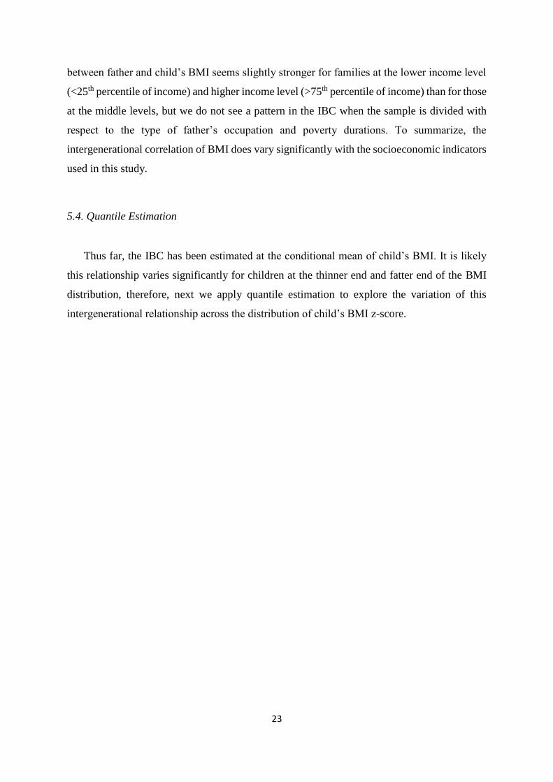
In this sample, there are 1,360 triple observations of children with father and mother. For
this restricted sample, using equation (1), the quantile estimates are displayed in Figure 6. They
suggest that for these children aged between 16 and 18 years old, the intergenerational
persistence in BMI z-score are highest at the fattest end of BMI distribution (with an estimate
of around 0.30 for father-child and 0.21 for mother-child). Compared with the pattern from the
full sample (Figure 5), we can see that the degree of intergenerational transmission in BMI z-
score varies with the stage of lifecycle, this motivates our analysis by age group in the next
section.
27
Figure 6: Quantile estimates of intergenerational correlation of BMI z-score on
Children aged 16-18 years old

28
5.6. Estimation by Age Group
We see the intergenerational correlation of BMI z-score varies with cohorts of different
life stages. In this respect our results may be sensitive to the age range over which children are
observed. To explore the change of this correlation with age, we estimate the intergenerational
correlation of BMI z-score separately by age group at two year intervals. The results are
provided in Table 8 and Figure 718. They suggest that this correlation increases until the children
are aged between eight and ten years old, when the estimates of the intergenerational BMI
correlation reach around 0.29 for father-child and 0.23 for mother-child. This increase is
followed by a decline over the rest of the childhood before the children enter adulthood for
mother-child, whereas a fluctuation for father-child. Therefore, the common environment and
genes that parents and child share together, play a greater role in the intergenerational
transmission of BMI when children are aged between 8-12 years old, than other childhood
stages prior to adulthood. One potential explanation is that before this pre-puberty stage, the
effects of inherited genes from their parents exert the maximum influence. Whereas, after this
stage, children spend less time with their parents, and exercise more control over their own
dietary and exercise choices and hence the effects of a common family environment decline.
Table 8 : OLS estimates of the intergenerational correlation of BMI by age group
Father and Child Mother and Child
Age Group (years) Obs Coefficient Std. Error Coefficient Std. Error
0-2 1,536 0.121*** 0.0452 0.243*** 0.0514
2-4 1,438 0.122*** 0.0386 0.153*** 0.0433
4-6 1,554 0.249*** 0.0356 0.257*** 0.0388
6-8 1,620 0.274*** 0.0333 0.238*** 0.0369
8-10 1,775 0.349*** 0.0314 0.302*** 0.0344
10-12 1,966 0.276*** 0.0291 0.280*** 0.0292
12-14 1,876 0.300*** 0.0262 0.268*** 0.0295
14-16 1,572 0.221*** 0.0248 0.217*** 0.0294
16-18 606 0.163*** 0.0449 0.0925** 0.0398
Note: the regression also includes: age dummies of child, gender of child and the interactions between them, father and mother’s age. Standard errors are clustered at the household level in parentheses, *** p<0.01, ** p<0.05,
* p<0.1
18 It should be remembered that this is the pooled sample, so each individual children can appear more than once
in the data as they age.

29
Figure 7 : Estimates of the intergenerational relatsionship of BMI z-score by age
group
0.1
.2.3
.4
0~2 4~6 8~10 12~14 16~18Age ( in years )
Coefficient Confidence Interval
Father-Child0
.1.2
.3.4
0~2 4~6 8~10 12~14 16~18Age ( in Years )
Coefficient 95% Confidence Interval
Mother-Child

30
6. Conclusions and Implications
Based on the CHNS longitudinal data from 1989 to 2009 and using BMI z-score as
the measure of adiposity, we estimate the intergenerational correlation of BMI z-score in
China. We use the OLS estimates as our baseline estimates of the intergenerational BMI
correlation, since it indicates the basic underlying intergenerational correlation, and it is
comparable with the intergenerational correlation of income or education, which are
mostly based on cross-section data. The OLS estimates suggest one standard deviation
increase in father’s BMI z-score is associated with an increase of 0.20 in child’s BMI z-
score, and this figure is around 0.22 for the correlation between mother and child’s BMI
z-score. These estimates decreases to around 0.14 for father-child and 0.12 for mother-
child when we control for the household fixed effects, similarly when we control for the
individual fixed effects. The fixed effects estimates provide some evidence for the rather
strong effects of short term environmental factors in the intergenerational transmission of
body weight.
0.1
.2.3
.4
0~2 4~6 8~10 12~14 16~18age_cat
Mother and Child
Father and Child
Parents-Child
31
We justifiably devoted considerable attention to the underlying observed
heterogeneity of this correlation. We found that this intergenerational correlation of BMI
does not vary substantially with family socio-economic indicators like: fathers occupation,
mothers education, family income or the amount of time recently spent in poverty. In
contrast, we did find that this correlation tends to be markedly higher among children
with higher BMI levels and lower with children below average BMI levels. In addition,
we found that this tendency becomes weaker when we use the sub-sample of children
approaching adulthood (i.e. children aged 16-18 years old). We also found some limited
evidence that there is a change of this intergenerational relationship during child’s
maturation. Specifically, that the correlation rises to a peak of around 27-29% between
the ages of 8 to 14 and subsequently falls back afterwards.
We may tentatively posit some policy implications of our findings – some of which
echo the literature - and some of which add nuance, and suggest some clearer directions
for policy than have been hitherto understated. The first finding of importance is that –
contrary to much recent conventional wisdom – a person’s BMI is not completely
determined by their own life style and decisions – some of it is determined as a child by
your parents through both your biological inheritance and your family environment. On
average, approximately 20% of what an individual’ BMI is comes from their mother and
20% comes from their father. We find that around half (20% of the total 40% effect) of
this is likely to be due to factors which are determined at birth by their parents. These are
pre-determined factors which do not change over a child’s life are obviously a mix of
biological, genetic and environmental factors induced by their parents. The other half of
our effects – the difference between the fixed effect and OLS estimates – result from
factors which do change inside the families over time. As suggested by others, there is
scope for interventions - at the level of the family - which may have a realistic chance of
having an effect (See Golan 2006). Specifically, one would wish to target parents of
children about healthy eating, nutrition and the importance of exercise (Graham and
Power 2004). This would be predicated on explaining to parents that they can have a
direct role in conditioning their children’s health outcomes which in turn will affect their
life chances (Nestle 2006, Golan 2006). The corollary of this implication is that
potentially the remaining 50-60% of the variance of what determines a child’s BMI (at
the conditional mean) is determined by factors that are outside the family. Our data also
suggests that family factors diminish slightly as a child approaches adulthood. This means

32
that a child’s own decisions (about nutrition and exercise) will become more important
as they grow older. The public health message of this is that an individual is still
responsible for the larger part of their own health outcomes. None of this is particularly
new – we have always known that this responsibility needs to be shared. What is slightly
newer though is the apportionment of the responsibility between the parents and the child
themselves and between things which the family give a child which cannot be changed
and the things which can be changed. Our research has put some tentative bounds on these
effects for Chinese children.
In examining the heterogeneity of our findings across the distribution of child’s BMI we
found that the picture is very different at different ends of the distribution. The fatter
children have around 30% of their BMI determined by each of their parents, the thin
children only 10% by each parent. This means we need to focus our public health
message by directly targeting the families most at risk.
Finally our findings which relate to the observed heterogeneity of the intergenerational
BMI by social class and economic circumstances of the parents are relatively reassuring
in that they suggest that, in China, there is no evidence of a ‘social gradient’ in the
transmission of obesity. This means that – unlike in the UK or US – there is no evidence
that obesity transmission is predominantly a problem of the poor. This finding means
that the targeting of government interventions do not need to be focussed in quite the
same way as they are in more developed countries. This prompts the observation that the
nutritional and epidemiological transformation which has hit China is coming much later
than in the West and – as a result – this means that the obesity epidemic which has hit the
US and other Western European countries may take a very different form in China –
specifically that it may hit all social classes relatively equally.
33
References
Ahlburg, D. (1998). Intergenerational transmission of health. American Economic Review, 88(2),
265-270.
Akbulut, M., and Kugler, A. D. (2007). Inter-generational transmission of health status in the US
among natives and immigrants. Mimeo (University of Houston). Retrieved from
http://www.uh.edu/~makbulut/akbulut_kugler_health.pdf
Anderson, P. M. (2012). Parental employment, family routines and childhood obesity. Economics
and Human Biology, 10(4), 340-351.
Anger, S., and Heineck, G. (2010). Do smart parents raise smart children? The intergenerational
transmission of cognitive abilities. Journal of Population Economics, 23(3), 1105-1132.
Becker, G. S., and Tomes, N. (1986). Human Capital and the Rise and Fall of Families.
Journal of Labor Economics, S1-S39.
Bell, A. C., Ge, K., and Popkin, B. M. (2012). The road to obesity or the path to prevention: motorized
transportation and obesity in China. Obesity Research , 10 (4), 277-283.
Bhalotra, S., and Rawlings, S. (2013). Gradients of the Intergenerational Transmission of
Health in Developing Countries. Review of Economics and Statistics, 95(02),
660-672.
Björklund, A., Roine, J., and Waldenström, D. (2012). Intergenerational top income mobility
in Sweden: Capitalist dynasties in the land of equal opportunity? Journal of Public
Economics, 96(5), 474-484.
Black, S. E., Devereux, P. J., and Salvanes, K. G. (2005). Why the Apple Doesn’t Fall Far:
Understanding Intergenerational Transmission of Human Capital. American Economic
Review, 95(1), 437–449.
Bouchard, C. and Perusse, L. (1994) Genetics of obseity: Family studies, chp 6 in The Genetics of
Obseity, ed Boucher, C. CRC Press Ann Arbor.
Classen, T. J. (2010). Measures of the intergenerational transmission of body mass index between
mothers and their children in the United States, 1981–2004. Economics and Human Biology,
8(1), 30-43.
Cole, Tim J., Katherine M. Flegal, Dasha Nicholls, and Alan A. Jackson. "Body mass
index cut offs to define thinness in children and adolescents: international
survey." British Medical Journal, 335, no. 7612 (2007): 194.

34
Coneus, K., and Spiess, C. K. (2012). The intergenerational transmission of health in early
childhood—Evidence from the German Socio-Economic Panel Study. Economics and Human
Biology, 10(1), 89-97.
Conley, D., and Bennett, N. G. (2000). Is biology destiny? Birth weight and life chances. American
Sociological Review, 65(3), 458-467.
Currie, J., and Moretti, E. (2007). Biology as Destiny? Short-and Long-Run Determinants of
Intergenerational Transmission of Birth Weight. Journal of Labor Economics, 25(2), 231-263.
Dasgupta, P. (1993). An Inquiry into Well-Being and Destitution. New York: Oxford University
Press Inc.
Dearden, L., Machin, S., and Reed, H. (1997). Intergenerational mobility in Britain. The
Economic Journal,107(440), 47-66.
Desai, S., and Alva, S. (1998). Maternal education and child health: Is there a strong causal
relationship?. Demography, 35(1), 71-81.
Dolton, P., and Xiao, M. (2015) The Intergenerational transmission of adiposity across countries,
University of Sussex, mimeo.
Doyle, O., Harmon, C. P., Heckman, J. J., & Tremblay, R. E. (2009). Investing in early human
development: timing and economic efficiency. Economics and Human Biology, 7(1), 1-6.
Du, S., Lu, B., Zhai, F., and Popkin, B. M. (2002). A new stage of the nutrition transition
in China. Public Health Nutrition, 5(1A), 169-174
Dubois,L, Kyvik, K, Girard, M., Tatone-Tokunda, F., Perusse, D. Hjelmborg,, Skytthe, A.,
Rasmussen, F., Wright, M., Lichtenstein, P. and Martin, N. (2012) Genetic and environmental
contributions to weight, height and BMI from bith to 19 years of age: An international study
over 12,000 twin pairs, PLoS ONE, 7(2), 1-12.
Emanuel, I., Filakti, H., Alberman, E., and Evans, S. J. (1992). Intergenerational studies
human birthweight from the 1958 birth cohort. 1. Evidence for a multigenerational
effect. BJOG: An International Journal of Obstetrics and Gynaecology, 99(1), 67-74.
Eriksson, T, Jay P, and Xuezheng, Q. “The Intergenerational Inequality of Health in
China.” China Economic Review 31, no.0 (2014): 392–409.
Fukagawa, N. K., Bandini, L. G., & Young, J. B. (1990). Effect of age on body composition and
resting metabolic rate. American Journal of Physiology, 259 (2 Pt 1), E233-E238.
Galton, F.(1869). Hereditary Genius: An Inquiry into Its Laws and Consequences. London:
Macmillan.

35
Galton, F.(1877). Typical Laws of Heredity. Proc. Royal Inst. Great Britain 8 (February 1877): 282–
301.
Golan, M. (2006). Parents as agents of change in childhood obesity‐from research to
practice. International Journal of Pediatric Obesity, 1(2), 66-76.
Goldberger, A. S. (1989). Economic and Mechanical Models of Intergenerational Transmission.
American Economic Review, 79(3), 504-513.
Gong, H., Leigh, A., and Meng, X. (2012). Intergenerational income mobility in urban China. Review
of Income and Wealth, 58 (3), 481-503
Gorber, S. C., Tremblay, M., Moher, D., and Gorber, B. (2007). A comparison of direct vs. self-report
measures for assessing height, weight and body mass index: a systematic review. Obesity
Reviews, 8(4), 307-326.
Graham, H., & Power, C. (2004). Childhood disadvantage and health inequalities: a framework for
policy based on lifecourse research. Child Care, Health and Development, 30(6), 671-678.
Gruber, J. (2009). The Problems of Disadvantaged Youth: An Economic Perspective: Chicago:
University of Chicago Press.
Guo, X., Mroz, T. A., Popkin, B. M., and Zhai, F. (2000). Structural change in the impact of income
on food consumption in China, 1989–1993. Economic Development and Cultural
Change, 48(4), 737-760.
Han, S., and Mulligan, C. B. (2001). Human capital, heterogeneity and estimated degrees of
intergenerational mobility. The Economic Journal, 111(470), 207-243
Heller, R., Garrison, R., Havlik, R., Feinleib, M. And Padgett, S. (1984) Family resemblences in
height and relative weight in the Frmalington Heart Study. International Journal of Obesity,
8, 399.
Kalmijn, M. (1994). Assortative mating by cultural and economic occupational status. American
Journal of Sociology, (100), 422-452.
Klein, L. R., and Ozmucur, S. (2003). The estimation of China's economic growth rate. Journal of
Economic and Social Measurement, 28(4), 187-202.
Knight, J., and Song, L. (2012). Towards a labour market in China. Oxford Review of Economic
Policy, 11(4), 97-117.
Laitinen, J., Power, C., and Järvelin, M. R. (2001). Family social class, maternal body mass index,
childhood body mass index, and age at menarche as predictors of adult obesity. American
Journal of Clinical Nutrition, 74(3), 287-294.
36
Li, L., Law, C., Lo Conte, R., and Power, C. (2009). Intergenerational influences on childhood body
mass index: the effect of parental body mass index trajectories. American Journal of Clinical
Nutrition, 89(2), 551-557.
Loureiro, M. L., Sanz‐de‐Galdeano, A., and Vuri, D. (2010). Smoking Habits: Like Father, Like Son,
Like Mother, Like Daughter? Oxford Bulletin of Economics and Statistics, 72(6), 717–743.
Maes, H., Neale, M., and Eaves, L. (1997) Genetic and environmental factors in relative body weight
and human adiposity, Behavior Genetics, 27(4), 325-351.
Mare, R. D. (1991). Five decades of educational assortative mating. American Sociological Review,
56(1), 15-32.
Martin, M. A. (2008). The intergenerational correlation in weight: how genetic resemblance reveals
the social role of families. American Journal of Sociology, 114(Suppl), S67-S105.
Moll, P., Burns, T., and Lauer, R. (1991) The genetic and environmental sources of body mass index
variability: The muscatine ponerosity Family Study, American Journal of Human Genetics,
49, 1243-1255.
Morgan, S. L. (2000). Richer and taller: stature and living standards in China, 1979-1995. The China
Journal, (44), 1-39.
Mulligan, C. B. (1999). Galton versus the human capital approach to inheritance. Journal of Political
Economy, 107(6 PART 2), S184-S224.
National Bureau of Statistics of China. (2012). Income of Urban and Rural Residents in 2011.
http://www.stats.gov.cn/tjfx/jdfx/t20120120_402780174.htm
Nestle, M. (2006) "Food marketing and childhood obesity—a matter of policy. "New England
Journal of Medicine 354, no. 24: 2527-2529.
Nickell, S. (1981). Biases in dynamic models with fixed effects. Econometrica, 49, 1417-1426.
Onis, Mercedes de, Adelheid W. Onyango, Elaine Borghi, Amani Siyam, Chizuru Nishida,
and Jonathan Siekmann. (2007) "Development of a WHO growth reference for school aged
children and adolescents." Bulletin of the World Health Organization 85, no. 9:
660-667.
Osmani, S., & Sen, A. (2003). The hidden penalties of gender inequality: fetal origins of ill-
health. Economics & Human Biology, 1(1), 105-121.
Perusse, L. Leblanc, C and Boucher, C. (1988) Inter-generation transmission of physical fitness in
the canadian populatio., Canadian Journal of Sports Science, 13, 8.
Pitt, M. M., Rosenzweig, M. R., and Hassan, M. N. (1990). Productivity, health, and
inequality in the intrahousehold distribution of food in low-income countries. The
37
American Economic Review, 80(5), 1139-1156.
Pollak, R. A. (2005). Bargaining power in marriage: Earnings, wage rates and household
production (No. w11239). National Bureau of Economic Research.
Popkin, B. M. (2001). The nutrition transition and obesity in the developing world. The Journal of
Nutrition, 131(3), 871S-873S.
Popkin, B. M. (2008). The nutrition transition: an overview of world patterns of change. Nutrition
Reviews, 62(s2), S140-S143.
Popkin, B. M., Du, S., Zhai, F., and Zhang, B. (2010). Cohort Profile: The China Health and Nutrition
Survey—monitoring and understanding socio-economic and health change in China, 1989–
2011. International Journal of Epidemiology, 39(6), 1435-1440.
Qian, N. (2008). Missing women and the price of tea in China: The effect of sex-specific earnings on
sex imbalance. The Quarterly Journal of Economics,123(3), 1251-1285.
Royer, H. (2009). Separated at birth: US twin estimates of the effects of birth
weight. American Economic Journal: Applied Economics, 1(1), 49-85.
Scholder, S. V. H. K., Smith, G. D., Lawlor, D. A., Propper, C., and Windmeijer, F. (2012). The effect
of fat mass on educational attainment: Examining the sensitivity to different identification
strategies. Economics and Human Biology, 10 (4),405-418.
Sherry, B., Jefferds, M. E., and Grummer-Strawn, L. M. (2007). Accuracy of adolescent self-report
of height and weight in assessing overweight status: a literature review. Archives of Pediatrics
and Adolescent Medicine, 161(12), 1154.
Smith, G. D., Steer, C., Leary, S., and Ness, A. (2007). Is there an intrauterine influence on obesity?
Evidence from parent–child associations in the Avon Longitudinal Study of Parents and
Children (ALSPAC). Archives of Disease in Childhood, 92(10), 876–880.
Song, S. (2013). Identifying the intergenerational effects of the 1959–1961 Chinese Great Leap
Forward Famine on infant mortality. Economics and Human Biology, 11(4), 474-487.
Spencer, E. A., Appleby, P. N., Davey, G. K., and Key, T. J. (2002). Validity of self-reported
height and weight in 4808 EPIC–Oxford participants. Public Health Nutrition, 5(04),
561-565.
Tafreschi, D. (2014). The income body weight gradients in the developing economy of
China. Economics and Human Biology. 16, 115-134.
Tambs, K. Moum, T., Eaves, L., Neale, M., Midthjell, K., Lund-Larsen, P., Naes, S. And Holmen, J.
(1991) Genetic and environmental contributions to the variance of the body mass index in a

38
Norwegian sample of first and second generation relatives. American Journal of Human
Biology, 3, 257.
Thomas, D. (1990). Intra-household resource allocation: An inferential approach. Journal
of Human Resources,25(4), 635-664.
Thompson, O. (2012).The Intergenerational Transmission of Health Status: Estimates
and Mechanisms. Ph.D Thesis. University of Wisconsin:U.S.
Trannoy, A., Tubeuf, S., Jusot, F., and Devaux, M. (2010). Inequality of opportunities in
health in France: a first pass. Health Economics, 19(8), 921-938.
Van de Poel, E., O’Donnell, O., & Van Doorslaer, E. (2009). Urbanization and the spread of
diseases of affluence in China. Economics and Human Biology,7(2), 200-216.
Wang, Youfa and Hsin-Jen Chen. "Use of Percentiles and Z-Scores in Anthropometry."
In Handbook of Anthropometry: Physical Measures of Human Form in Health and
Disease, ed.Victor R. Preedy, pp. 29-48. Springer Science+Business Media, LLC, New York,
2012.
WHO, E. C. (2004). Appropriate body-mass index for Asian populations and its implications for
policy and intervention strategies. Lancet, 363(9403), 157.
Wong, Edward. "‘Reports of Forced Abortions Fuel Push To End Chinese Law." New York
Times 22 (2012).
Wu, Y. (2006). Overweight and obesity in China. British Medical Journal, 333(7564), 362-
363

39
Appendix A.
Figure A1: Map of China Health and Nutrition Survey (CHNS) Regions
Note: The darker shaded regions are the provinces in which the survey has been conducted. They are:
Guangxi; Guizhou; Heilongjiang; Henan; Hubei; Hunan; Jiangsu; Liaoning; Shandong.
http://www.cpc.unc.edu/projects/china/proj_desc/chinamap; the CHNS data is not nationally
representative, rather, this is a purposeful sample of selected provinces and within the provinces, counties
and large urban areas. Thus, this result does not provide representativeness at the national, provincial or
community levels.

40
Some descriptive statistics of the CHNS data
Table A 2 displays the number of parent-child pairs that were observed for multiple times.
These repeated observations facilitate the possibility of netting out for time-invariant
unobserved individual heterogeneity through individual fixed effects.
Table A1: The number of times that children were observed in CHNS
(1989-2009)
Waves 1 2 3 4 5 6 7 Total
Numbers of children 1,840 1,933 1,164 707 352 45 3 6044
Frequency of Observations 1,840 3,866 3,492 2,828 1,760 270 21 14077
Note: In this longitudinal data, 1,840 individuals are observed for one wave, 1,933 individuals
are observed for two waves, the sum of observations is 14,077.
Table A2: Summary of BMI z-score when they were observed for
the last time.
19 Due to the potential error in data recording for height and/or weight, some children’s BMI z-scores are
considered as biologically implausible and flagged as missing by the Anthro software. In addition, we drop
BMI z-scores outside of the commonly applied range (-5, 5).
Obs Mean Std.
Dev.
Min Max
Father
Age 6044 40.28 6.77 18.97 69.66
Height 6044 166.42 6.39 144.8 189
Weight 6044 62.70 10.08 38 115.3
BMI 6044 22.58 2.93 13.06 36.39
BMI z-score 6044 0.019 0.96 -4.64 3.15
Mother
Age 6044 38.64 6.32 19.57 66.01
Height 6044 155.89 5.78 131 175.5
Weight 6044 55.17 8.71 33.2 98
BMI 6044 22.66 3.06 15.08 41.32
BMI z-score 6044 0.28 0.87 -2.79 3.79
Child
Age 6044 12.28 4.438 0.02 17.99
Height 6044 142.87 24.50 50 186
Weight 6044 38.66 15.08 3.2 97.7
BMI 6044 18.02 2.89 10.74 39.07
BMI z-score 602819 -0.35 1.19 -4.85 5

41
Table A3: Summary of height, weight and BMI z-score (from Pooled Data)
Table A 2 presents the basic summary statistics of the maximum number of complete sets
of child, mother and father the last survey time we observe them, Table A 3 presents the
summary statistics of the pooled observations. They suggest that the Chinese are still,
predominantly shorter and lighter than people in developed western countries, but there
is still a high variance to be explained.
Obs Mean Std.
Dev.
Min Max
Father
Age 14077 37.51 6.93 18.97 69.66
Height 14077 166.22 6.26 144.8 189
Weight 14077 61.49 9.49 38 115.3
BMI 14077 22.20 2.76 13.06 36.39
BMI z-score 14077 -0.10 0.93 -4.64 3.15
Mother
Age 14077 35.92 6.50 18.31 66.01
Height 14077 155.70 5.68 131 179
Weight 14077 54.11 8.36 32.5 98
BMI 14077 22.28 2.93 14.72 41.32
BMI z-score 14077 0.169 0.85 -3 3.79
Child
Age 14077 9.59 4.78 0.02 17.99
Height 14077 128.01 27.84 50 186
Weight 14077 30.02 15.01 3.2 97.7
BMI 14077 17.07 2.72 10.74 39.07
BMI z-score 14006 -0.21 1.25 -4.99 5.38

42
Figure A4. (a) BMI z-score of child aged <= 6 over time.
Figure A4 (b) BMI z-score of child aged 7-12 over time.
0.1
.2.3
.4
kd
en
sity
-5 0 5BMI-age-zscore
child<=6 1989,1991,1993 child<=6 1997,2000
child<=6 2004,2006,2009
BMI z-score of Child aged<=6 over time
0.1
.2.3
.4
Kd
en
sity
-5 0 5BMI-age-zscore
child 7~12 1989,1991,1993 child 7~12 1997,2000
child 7~12 2004,2006,2009
BMI z-score of child aged 7-12 over time

43
Figure A4 (c) BMI z-score of child aged 13-18 over time.
Figure A5 BMI z-score of father over time
0.1
.2.3
.4
kd
en
sity
-5 0 5BMI-age-zscore
child 13~18 1989,1991,1993 child 13~18 1997,2000
child 13~18 2004,2006,2009
BMI z-score of child aged 13-18 over time
underweight
overweight
obese
0.1
.2.3
.4.5
kd
en
sity
-4 -2 0 2 4BMI-age-zscore
father 1989,1991,1993 father 1997,2000
father 2004,2006,2009
BMI z-score of father over time

44
Figure A5 BMI z-score of mother over time
underweight overweight
obese
0.1
.2.3
.4.5
kd
en
sity
-4 -2 0 2 4BMI-age-zscore
mother 1989,1991,1993 mother 1997,2000
mother 2004,2006,2009
BMI z-score of mother over time

45
Appendix B: The Metrics and Magnitudes of BMI z-score and logBMI
Intergenerational Correlations.
There is some disagreement in what is the correct measure of adiposity to use in statistical
work on intergenerational transmission. In this appendix we clarify the alternative
measures that have been used, their inter-relationship and their relative merits and
disadvantages.
The Different Measures of Adiposity used in Statistical and Econometric Research.
The most common measures of adiposity 20 used is statistical relations between one
generation and another are:
i) The raw BMI,
ii) The BMI z-score relative to some population.
iii) The log of the BMI.
In thinking about how to compare the relative merits of these measures it should be
remembered that the BMI measure is itself a specific non-linear measure of height and
weight, defined as: [weight(kg)/height2(cm)]*10,000. This means that transformations
of the BMI need to be treated with care. In consequence, coefficients of regressions
involving transformations of this ratio – especially when normed against a reference
population - can be difficult to interpret and compare. Inevitably their interpretation also
depends on what controlling regressors have been used in the estimation. All these factors
contribute to difficulties in comparing coefficients across different published research
findings.
Predominantly the medical, biological and epidemiological literature has mainly
estimated an intergenerational BMI correlation (IBC) which is the size of the either the
raw correlation of fathers BMI, 𝑦𝐹 , with child’s BMI21, 𝑦𝑐 , or the coefficient, 𝛽1 , in
equation (B1) of the regression of child’s BMI on fathers BMI.
𝑦𝑐 = 𝛼1 + 𝛽1𝑦𝐹 + 𝑢1 (B1)
20 Some medical studies have access to other measure like percentage body fat or measures of skin
pinches. This data was not available to this study. 21 For the sake of simplicity we use the example of child and father in this Appendix – the same logic
applies to mother and child.

46
Fortunately, if the simple regression in (B1) is transformed into z-score values the
interpretation of the IBC coefficient, 𝛽1 , does not change much to, 𝛽2 in equation (B2).
𝑍𝑐 = 𝛼2 + 𝛽2𝑍𝐹 + 𝑢2 (B2)
where 𝑧 =𝑦−�̅�
𝜎
Indeed it can be shown by simple algebra that 𝛽1 = 𝜎𝛽2 (under basic regularity
conditions).
This means that the marginal effects interpretation of the IBC coefficient is very similar
in equation (B1) and (B2). Specifically in equation B2, the IBC estimate will be the effect
of a one unit change of the standard deviation of the fathers BMI z-score on the child’s
BMI z score. This means, that broadly speaking the IBC estimates from basic raw BMI
regressions and those run in z-scores are comparable – relative to the reference group
which norms these BMI values. (We discuss this below.)
Where the position becomes more complicated is when we use the logBMI as the variable
in our regression. Specifically if we run the regression:
𝑙𝑜𝑔𝑦𝑐 = 𝛼3 + 𝛽3𝑙𝑜𝑔𝑦𝐹 + 𝑢1
then the comparison of 𝛽3 with 𝛽1 or 𝛽2 is slightly more problematic. The reason we
might want to do that is to compare the marginal effect in the coefficient 𝛽3 – which is
now an elasticity – indeed we can call the this the intergenerational BMI elasticity, IBE
– with the literature on estimating the elasticity of transmission across generations. This
elasticity has been estimated by many papers and it would be insightful to be able to
compare this IBE with the corresponding estimates of elasticity of intergenerational
transmission of income or education. Our difficulty is that this is not what has been
estimated by the epidemiological literature on the intergenerational transmission of
adiposity – here an IBC has been estimated. This is why we have chosen to present these
estimates in this paper. For completeness the IBC estimates are provided in an Appendix
C (available to readers on request) in which the equation estimated in (B3) and its
analogues with controls.
So, the logical question is – how might the IBC and IBE compare for the same data. This
is particularly important if we wish to compare our estimates with those of Classen (2010),
as he estimates an IBE. The answer is that the IBE will typically be non-comparable with

47
the IBC. What is logically the case is that the IBC will typically be less than the IBE –
but this is not surprising as the IBC is based on a regression which has been transformed
in natural logs so that the metric of adiposity are much smaller numbers. There is no
uniform look up comparison possible though as the estimated intercept needs to be taken
into account. Explicitly it should be remembered that the log transformation is a specific
non-linear transformation (which makes appropriate the proportionate change
interpretation consistent with an elasticity). To see this we can verify with a numerical
example from our data. Using our data from Table A3 and Table 1, column 1 and Table
C1 column 1 we can verify the property that the z-score regression goes through the mean
of the data:
2 2ˆˆ
c FZ Z
-0.21 = -0.190 + .223(-0.10)
Likewise, using our data from Table A3 and Table C1 column 1 we can verify the
property that the double log regression goes through the mean of the data:
3 3l ˆg gˆo loc Fy y
Log(17.07) = 1.926 + .291 log(22.2)
This is conformation that our relative estimates of an IBC of .223 and an IBE of .291 are
comparable. This means that Classen’s (2010) estimate of an IBE of .35 needs to be
potentially considerably tempered in comparing it with or own IBC estimates which we
use in this paper. We provide in Appendix C a full set of results – directly analogous to
those in each table of the paper for those who may prefer to think in terms of an IBE
rather than an IBC. This is a matter of personal preference – but one that should be
informed by a comparison of the two different numbers for the same data.
The reader should keep in mind the distinction when comparisons with other papers are
made. The disadvantage of the double log transformation is that it is a particular non-
linear transformation (on an already transformed BMI variable) which makes
interpretation of the effects more difficult. The disadvantage of using the z-score method
is that it will depend on the validity of the reference group 22. Notwithstanding this
disadvantage we need to discuss this alternative in some more detail.
Using the BMI z-score Measure based on WHO reference group.
22 We also need to be careful in handling data in terms of z-scores as obviously approximately half of
these values are negative.
48
BMI z-scores are computed based on the comparison with reference population in
terms of mean and standard deviation. In this paper, the reference population comes from
the World Health Organization (WHO), there are three main versions of references: the
1978 WHO/NCHS Growth References (for children up to age10), the WHO Growth
References (for children and adolescents up to age 19), and the 2006 WHO Growth
Standards (for preschool children, under 6 years of age) (Wang and Chen 2012).
Most of the earlier versions are based on growth references developed and used in
the US. For 1978 WHO/NCHS (National Center for Health Statistics), the growth
reference for infants was developed based on data collected from the Fels Longitudinal
study, which followed mainly formula-fed children in Ohio State in the USA (Wang and
Chen, 2012). In 2006, WHO generate the 2006 WHO Child Growth Standards for which
the data was collected from Brazil, Ghana, India, Norway, Oman, and the USA. In 2007,
the 2007 WHO reference was released for children and adolescents aged 5 to 19 years,
using the same sample as for the 1978 WHO/NCHS growth references (Onis 2007). Thus,
the references used in this paper are the 2006 WHO Child Growth Standards for preschool
children under 5 years of age and the 2007 WHO Growth Reference for school-age
children and adolescent aged 5 to 19 years of age.
In Stata, the BMI zscores are calculated using the igrowup_standard.ado file
downloaded from the WHO website 23 . This file calculates z-scores for eight
anthropometric indicators based on the WHO Child Growth Standards, body mass index
(BMI)-for-age is one of them. The macro produces sex- and age-specific estimates for the
prevalence of under/over nutrition and summary statistics (mean and SD) of the z-scores
for each indicator. Extreme (i.e. biologically implausible) BMI z-scores (less than -5 and
more than 5) are flagged.
The BMI z-score system assumes the BMI values to be normally distributed and
computes the z-score based on the formula 𝑧 =𝑦−�̅�
𝜎, where 𝑦 is the individual’s BMI
value , 𝜇 is the mean BMI value of reference population , and 𝜎 is the standard deviation
of reference population, here the reference population refers to the sample from the WHO
23 They can be downloaded from http://www.who.int/childgrowth/software/en/ for Child growth
standards (0~5 years old) and http://www.who.int/growthref/tools/en/ for Growth reference (5~19 years
old).

49
macro software24. Thus, the anthropometric measure is expressed as a range of standard
deviations or z-scores above or below the mean or median value of reference population.
The BMI z-score adjusts the BMI value for age and gender, thus it is more comparable
across ages and genders compared to BMI values which are age and gender independent
(Wang and Chen 2012). In the conversion of BMI z-score, since the maximum age
available for 2007 WHO reference is 19 years old, the age of parents over 19 years old
will be treated as 19-year when their BMI z-scores are calculated, in other words, we
assume that parents’ BMI z-score follows the distribution of reference population aged
19 years old if the parents are over 19 years old. In addition, due to the potential error in
data recording for height and/or weight, some children’s BMI z-scores (below -5 and
above 5) are considered as biologically implausible and flagged as missing by the Anthro
software.
However, Note most of the papers argue that BMI is better than z-score, and z-score
makes things more complicated. Cole (2007) argues that BMI or BMI % are more
appropriate scales than BMI z-scores to measure the changes in adiposity, as the within-
child variability over time depends on the child’s level of adiposity rather than the relative
position to the reference population. Though in the case of a single cross section, BMI z-
score is a better measure for the level of adiposity.
24 It is argued that it might not be appropriate to use the WHO criteria to apply to some populations in the
Western Pacific Region due to their anthropometric characteristics.

50
Appendix C.
Corresponding results using raw BMI (rather than BMI z-score)
Instead of BMI z-score, we also estimate the intergenerational elasticity of BMI using
the log of raw BMI based on formula BMI = [weight(kg)
height2(cm)] ∗ 10,000, controlling for age,
age square, gender of child, the interactions between them and the age of father and
mother. The results are presented below, they suggest the results of intergenerational
elasticity of BMI are consistent with those of intergeneration correlation of BMI z-score .
This consistency implies that the intergeneration correlation of adiposity is robust to the
measure of adiposity.
Table C1: OLS estimates of the intergenerational BMI elasticity
(1) (2) (3) (4) (5)
Dependent variable: Log(BMI of child)
Log (BMI of Father) 0.291*** 0.238*** 0.211*** 0.210***
(0.013) (0.013) (0.012) (0.012)
Log (BMI of Mother) 0.282*** 0.234*** 0.173*** 0.174***
(0.012) (0.012) (0.011) (0.011)
Age of Child -0.035*** -0.034***
(0.001) (0.001)
(Age of Child)2/100 0.267*** 0.267***
(0.005) (0.005)
Male 0.027*** 0.027***
(0.005) (0.005)
Age*Male -0.002*** -0.002***
(0.000) (0.000)
Father’s age -0.001
(0.000)
Mother’s age 0.000
(0.000)
Constant 1.926*** 1.954*** 1.363*** 1.665*** 1.680***
(0.040) (0.037) (0.050) (0.046) (0.046)
Observations 14,082 14,082 14,082 14,082 14,082
R-squared 0.053 0.056 0.090 0.355 0.355
Notes: Robust standard errors in parentheses, standard errors clustered at individual level, *** p<0.01,
** p<0.05, * p<0.1
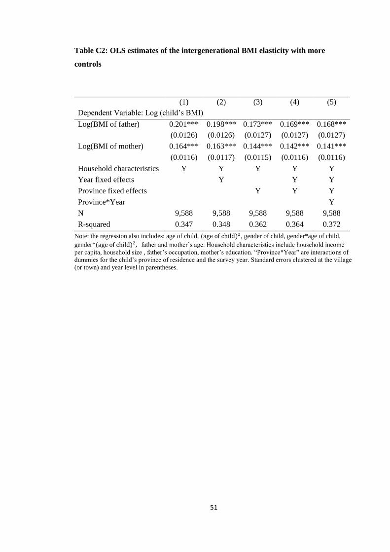
51
Table C2: OLS estimates of the intergenerational BMI elasticity with more
controls
(1) (2) (3) (4) (5)
Dependent Variable: Log (child’s BMI)
Log(BMI of father) 0.201*** 0.198*** 0.173*** 0.169*** 0.168***
(0.0126) (0.0126) (0.0127) (0.0127) (0.0127)
Log(BMI of mother) 0.164*** 0.163*** 0.144*** 0.142*** 0.141***
(0.0116) (0.0117) (0.0115) (0.0116) (0.0116)
Household characteristics Y Y Y Y Y
Year fixed effects Y Y Y
Province fixed effects Y Y Y
Province*Year Y
N 9,588 9,588 9,588 9,588 9,588
R-squared 0.347 0.348 0.362 0.364 0.372
Note: the regression also includes: age of child, (age of child)2, gender of child, gender*age of child,
gender*(age of child)2, father and mother’s age. Household characteristics include household income
per capita, household size , father’s occupation, mother’s education. “Province*Year” are interactions of
dummies for the child’s province of residence and the survey year. Standard errors clustered at the village
(or town) and year level in parentheses.

52
Table C3: OLS estimates of the intergenerational BMI elasticity, controlling for
the lagged value of Child’s BMI
(1) (2) (3)
Dependent variable: Log(BMI of child)
Log (BMI of Father) 0.211*** 0.169*** 0.169***
(0.013) (0.011) (0.011)
Log (BMI of Mother) 0.195*** 0.135*** 0.135***
(0.012) (0.011) (0.011)
Age of Child -0.004** -0.004**
(0.002) (0.002)
(Age of Child)2/100 0.116*** 0.116***
(0.009) (0.009)
Male 0.025*** 0.025***
(0.007) (0.007)
Age*Male -0.0027*** -0.002***
(0.001) (0.001)
Father’s age -0.0001
(0.000)
Mother’s age -0.0003
(0.000)
Log (Child’s BMI in t-1) 0.471*** 0.384*** 0.384***
(0.014) (0.014) (0.014)
Constant 0.259*** 0.718*** 0.731***
(0.056) (0.057) (0.057)
Observations 8,037 8,037 8,037
R-squared 0.274 0.487 0.487
Notes: Robust standard errors in parentheses, standard errors clustered at
individual level, *** p<0.01, ** p<0.05, * p<0.1

53
Table C4: Fixed Effects Estimates of the intergenerational elasticity
(1) (2) (3) (4)
Individual
Fixed
Effects
Individual
Fixed
Effects
Household
Fixed
Effects
Household
Fixed
Effects
Dependent variable: Log(BMI of child)
Log (BMI of father) 0.130*** 0.138*** 0.140*** 0.148***
(0.024) (0.024) (0.023) (0.023)
Log(BMI of mother) 0.124*** 0.131*** 0.110*** 0.116***
(0.023) (0.023) (0.021) (0.021)
Obese father*mother -0.013 -0.006
(0.118) (0.116)
Underweight father*mother 0.012** 0.013**
(0.006) (0.006)
Age of Child -0.0334*** -0.033*** -0.036*** -0.036***
(0.005) (0.006) (0.001) (0.001)
(Age of Child)2/100 0.277*** 0.276*** 0.271*** 0.270***
(0.006) (0.006) (0.006) (0.006)
Male of Child 0.030*** 0.030***
(0.006) (0.006)
Male*Age of Child -0.003*** -0.003*** -0.003*** -0.003***
(0.001) (0.001) (0.001) (0.001)
Age of Father 0.008 0.008 0.005*** 0.005***
(0.005) (0.005) (0.002) (0.002)
Age of Mother -0.010* -0.010* -0.004** -0.004**
(0.005) (0.005) (0.002) (0.002)
Constant 2.118*** 2.075*** 2.052*** 2.005***
(0.170) (0.171) (0.083) (0.086)
Observations 14,082 14,082 14,014 14,014
Number of individuals 6,045 6,045
Number of households 3,711 3,711
R-squared 0.399 0.399 0.356 0.356
Notes: Robust standard errors in parentheses, standard errors clustered at individual level, *** p<0.01,
** p<0.05, * p<0.1
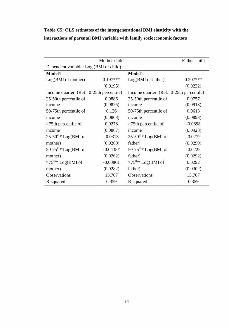
54
Table C5: OLS estimates of the intergenerational BMI elasticity with the
interactions of parental BMI variable with family socioeconomic factors
Mother-child
elasticity
Father-child
elasticity Dependent variable: Log (BMI of child)
Model1 Model1
Log(BMI of mother) 0.197*** Log(BMI of father) 0.207***
(0.0195) (0.0232)
Income quarter: (Ref.: 0-25th percentile)
of Income)
Income quarter: (Ref.: 0-25th percentile)
of Income) 25-50th percentile of
Income
0.0886 25-50th percentile of
Income
0.0757
income (0.0825) income (0.0913)
50-75th percentile of
Income
0.126 50-75th percentile of
Income
0.0613
income (0.0803) income (0.0893)
>75th percentile of
Income
0.0278 >75th percentile of
Income
-0.0898
income (0.0867) income (0.0928)
25-50th* Log(BMI of
mother)
-0.0313 25-50th* Log(BMI of
father)
-0.0272
mother) (0.0269) father) (0.0299)
50-75th* Log(BMI of
mother)
-0.0435* 50-75th* Log(BMI of
father)
-0.0225
mother) (0.0262) father) (0.0292)
>75th* Log(BMI of
mother)
-0.00861 >75th* Log(BMI of
father)
0.0292
mother) (0.0282) father) (0.0302)
Observations 13,707 Observations 13,707
R-squared 0.359 R-squared 0.359

55
Mother-child
elasticity
Father-child
elasticity Dependent variable: Log (BMI of child)
Model 2 Model 2
Log( BMI of mother) 0.215*** Log (BMI of father) 0.174***
(0.0121) (0.0158)
Highest degree: (Ref.: Primary and less) Occupation: (Ref.: famer)
High school 0.00656 Skilled/non-
skilled/service
worker and other
-0.131*
(0.0720) skilled/service (0.0701)
Technical and Tertiary 0.178 Professional/
administrator/executi
ve/manager/office
-0.0879
(0.139) technical/executive/
(0.0952)
administrative
High school* log (BMI of
mother)
0.000494 Skilled/non-skilled
skilled/service
worker and other*
Log(BMI of father)
0.0432*
mother) (0.0233) *log (BMI of father) (0.0228)
Technical and Tertiary*
Log(BMI of mother)
-0.0498 Professional/
xecutive/manager/off
ice* Log(BMI of
father)
0.0328
log (BMI of mother) (0.0448) *log (BMI of father)
(0.0307)
Observations 10,346 Observations 13,237
R-squared 0.339 R-squared 0.360

56
Mother-child
elasticity
Father-child
elasticity Dependent variable: Log (BMI of child)
Model 3 Model 3
Log (BMI of mother) 0.206*** Log (BMI of father) 0.182***
(0.0107) (0.0183)
The proportion of time in
poverty over the survey
years: (Ref.: 75%-100%
of time in poverty)
The proportion of time
in poverty over the
survey years: (Ref.:
75%-100% of time in
poverty)
50-75% of time in
poverty
0.101 50-75% of time in
poverty
-0.0730
poverty (0.102) poverty (0.110)
1-50% of time in poverty 0.163* 1-50% of time in poverty 0.0537
(0.0878) (0.103)
Never in poverty 0.0707 Never in poverty -0.135*
(0.0662) (0.0710)
50-75% of time in
poverty* Log(BMI of
mother)
-0.0333 50-75% of time in
poverty *Log (BMI of
father)
0.0233
Poverty*log (BMI of (0.0331) Poverty*log (BMI of (0.0358)
mother) mother)
1-50% of time in
poverty* Log (BMI of
mother)
-0.0534* 1-50% of time in
poverty* Log (BMI of
father)
-0.0178
Poverty*log (BMI of (0.0285) Poverty*log (BMI of (0.0334)
mother) mother)
Never in poverty*
Log(BMI of mother)
-0.0214 Never in poverty*
father)
0.0453*
log (BMI of mother) (0.0215) log (BMI of mother) (0.0231)
Observations 14,082 Observations 14,082
R-squared 0.356 R-squared 0.356
Notes: the regression also includes: age of child, (age of child)2, gender of child, gender*age of child,
gender*(age of child)2, father and mother’s age. Standard errors clustered at the village (or town) and
year level in parentheses.

57
Table C6: OLS estimates of the intergenerational BMI elasticity between mother
and child by SES measures: by income level, mother’s education and world
poverty line
Notes: Robust standard errors in parentheses, standard errors clustered at individual level, *** p<0.01, **
p<0.05, * p<0.1
Table C 7: OLS estimates of the intergenerational BMI elasticity between father
and child by SES measures: by income level, father’s occupation and world
poverty line
Sample
size
Elasticity Std.
Error
R-
squared <25th percentile of Income 3,323 0.204*** 0.0235 0.349
25-50th percentile of Income 3,462 0.182*** 0.0207 0.372
50-75th percentile of Income 3,461 0.190*** 0.0193 0.375
>75th percentile of Income 3,461 0.233*** 0.0208 0.327
Professional/technical/
administrator/executive/manager/office
1,811 0.203*** 0.0298 0.311
Skilled/non-skilled/service worker and
other
4,347 0.223*** 0.0188 0.347
Farmer 7,079 0.174*** 0.0164 0.378
75-100% of time in poverty 4,796 0.177*** 0.0202 0.394
50-75% of time in poverty 1,522 0.217*** 0.0349 0.276
1-50% of time in poverty 1,481 0.171*** 0.0297 0.296
Never in poverty 6,283 0.229*** 0.0160 0.341
Robust standard errors in parentheses, standard errors clustered at individual level, *** p<0.01,
** p<0.05, * p<0.1
Sample size Elasticity Std. Error R-squared
<25th percentile of Income 3,323 0.194*** 0.0188 0.349
25-50th percentile of Income 3,462 0.171*** 0.0190 0.372
50-75th percentile of Income 3,461 0.159*** 0.0191 0.375
>75th percentile of Income 3,461 0.186*** 0.0230 0.327
Primary school 3,250 0.176*** 0.0201 0.3784
High school 6,457 0.174*** 0.0169 0.3265
Technical and Tertiary 639 0.139*** 0.0478 0.2801
75-100% of time in poverty 4,796 0.194*** 0.0167 0.394
50-75% of time in poverty 1,522 0.170*** 0.0364 0.276
1-50% of time in poverty 1,481 0.144*** 0.0258 0.296
Never in poverty 6,283 0.167*** 0.0165 0.341
58
Figure C1: Quantile estimates of the intergenerational BMI elasticity

59
Figure C2: Quantile estimates of the intergenerational BMI elasticity on Children
aged 16~18 years old
Table C 8: Estimates of the intergenerational BMI elasticity by age group
Age Stage
(years)
Obs Father and Child (s.e) Mother and Child (s.e)
0-2 1551 0.087*** 0.0137***
2-4 1448 0.081*** 0.093***
4-6 1634 0.186*** 0.156***
6-8 1623 0.221*** 0.163***
8-10 1783 0.306*** 0.214***
10-12 1976 0.257*** 0.213***
12-14 1882 0.273*** 0.227***
14-16 1576 0.208*** 0.182***
16-18 609 0.158*** 0.095***
Notes: Robust standard errors in parentheses, standard errors clustered at individual level, *** p<0.01,
** p<0.05, * p<0.1
60
Figure C3: Estimates of the intergenerational BMI elasticity by age group
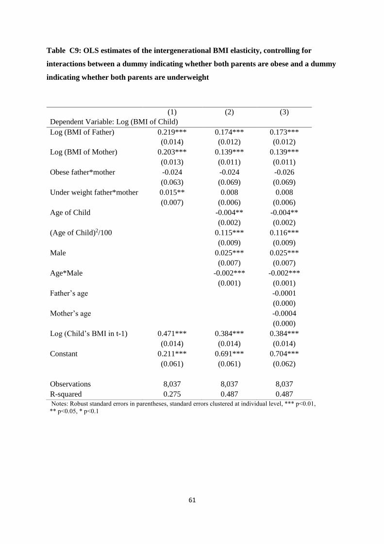
61
Table C9: OLS estimates of the intergenerational BMI elasticity, controlling for
interactions between a dummy indicating whether both parents are obese and a dummy
indicating whether both parents are underweight
(1) (2) (3)
Dependent Variable: Log (BMI of Child)
Log (BMI of Father) 0.219*** 0.174*** 0.173***
(0.014) (0.012) (0.012)
Log (BMI of Mother) 0.203*** 0.139*** 0.139***
(0.013) (0.011) (0.011)
Obese father*mother -0.024 -0.024 -0.026
(0.063) (0.069) (0.069)
Under weight father*mother 0.015** 0.008 0.008
(0.007) (0.006) (0.006)
Age of Child -0.004** -0.004**
(0.002) (0.002)
(Age of Child)2/100 0.115*** 0.116***
(0.009) (0.009)
Male 0.025*** 0.025***
(0.007) (0.007)
Age*Male -0.002*** -0.002***
(0.001) (0.001)
Father’s age -0.0001
(0.000)
Mother’s age -0.0004
(0.000)
Log (Child’s BMI in t-1) 0.471*** 0.384*** 0.384***
(0.014) (0.014) (0.014)
Constant 0.211*** 0.691*** 0.704***
(0.061) (0.061) (0.062)
Observations 8,037 8,037 8,037
R-squared 0.275 0.487 0.487
Notes: Robust standard errors in parentheses, standard errors clustered at individual level, *** p<0.01,
** p<0.05, * p<0.1
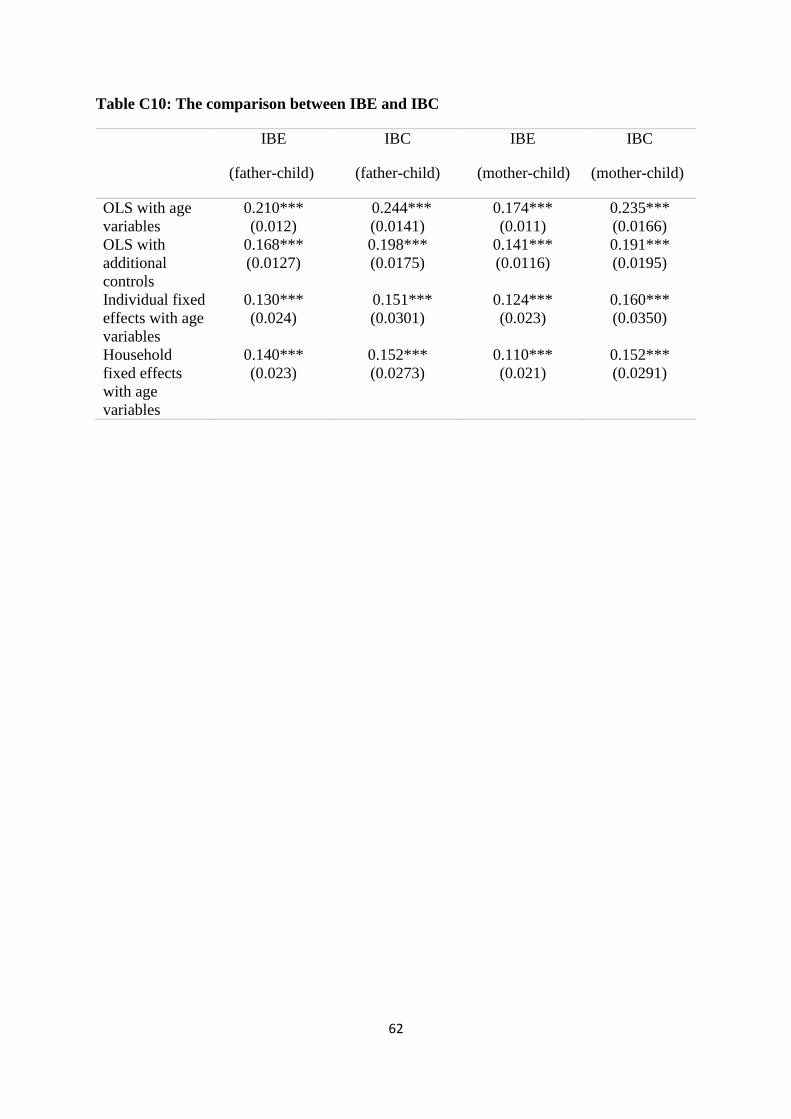
62
Table C10: The comparison between IBE and IBC
IBE
(father-child)
IBC
(father-child)
IBE
(mother-child)
IBC
(mother-child)
OLS with age
variables
0.210***
(0.012)
0.244***
(0.0141)
0.174***
(0.011)
0.235***
(0.0166)
OLS with
additional
controls
0.168***
(0.0127)
0.198***
(0.0175)
0.141***
(0.0116)
0.191***
(0.0195)
Individual fixed
effects with age
variables
0.130***
(0.024)
0.151***
(0.0301)
0.124***
(0.023)
0.160***
(0.0350)
Household
fixed effects
with age
variables
0.140***
(0.023)
0.152***
(0.0273)
0.110***
(0.021)
0.152***
(0.0291)


![[B3] XIAO Guangrui_TF 2012 Xiao Sichuan Roads Development Projects](https://img.pdfslide.us/doc/110x75/577ce47b1a28abf1038e7451/b3-xiao-guangruitf-2012-xiao-sichuan-roads-development-projects.jpg)