Embed Size (px)
Citation preview

vieS 4115
POLICY RESEARCH WORKING PAPER 2745
Children's W ork Econometric analysis basedon panel data from Peru finds
and Schooling: that changes in household
Does Gender M atter? welfare affect girls' work andschooling more than boys'.
Evidence from the Peru LSMSPanel Data
Nadeem Ilahi
The World Bank
Latin America and the Caribbean Region
Gender Sector Unit
December 2001
Pub
lic D
iscl
osur
e A
utho
rized
Pub
lic D
iscl
osur
e A
utho
rized
Pub
lic D
iscl
osur
e A
utho
rized
Pub
lic D
iscl
osur
e A
utho
rized
Pub
lic D
iscl
osur
e A
utho
rized
Pub
lic D
iscl
osur
e A
utho
rized
Pub
lic D
iscl
osur
e A
utho
rized
Pub
lic D
iscl
osur
e A
utho
rized
POLICY RESEARCH WORKING PAPER 2745
Summary findlingsUsing panel data from Peru, Ilahi investigates the welfare than does boys'. Similarly, girls are more likelydeterminants of the allocation of boys' and girls' time to than boys to adjust their home time in response toschooling, housework, and income-generating activities. changes in adult female employment and to sickness ofSpecifically, she explores whether sickness, female household members. Lack of access to energyheadship, access to infrastructure, and employment of infrastructure lowers the educational attainment of bothwomen in the household have different impacts on the boys and girls but has little affect on their labor.time use of boys and girls. The traditional approach to the determinants of child
Girls mostly engage in housework, and boys mostly labor and education excludes housework and maywork outside the home. As a work activity, housework understate children's time use, particularly that of girls.responds to economic incentives and constraints. It may therefore also overlook an important gender
The author's econometric findings suggest that changes dimension of education policy. Safety nets that protectin household welfare affect girls' work and schooling household incomes from employment shocks andmore than boys'. Even though boys' and girls' sickness, and childcare programs that allow women toeducational attainment rates are the same, girls' work, would reduce the likelihood of girls being pullededucation responds more to changes in household out of school.
This paper-a product of the Gender Sector Unit, Latin America and the Caribbean Region-was originally written for therecentWorld Bank publication EngenderingDevelopment. Copies of the paper are available free from the World Bank, 1818H Street NW, Washington, DC 20433. Please contact Selpha Nyairo, room 18- 11 0, telephone 202-473-4635, fax 202-522-0054, email address [email protected]. Policy Research Working Papers are also posted on the Web at http://econ.worldbank.org. December 2001. (37 pages)
The Policy Research Working Paper Series disseminates the findings of work in progress to encourage the exchange of ideas aboutdevelopment issues. An objective of the series is to get the findings out quickly, even if the presentations are less than fully polished. Thepapers carry the names of the authors and should be cited accordingly. The findings, interpretations, and conclusions expressed in this
paper are entirely those of the authors. They do not necessarily represent the view of the World Bank, its Executive Directors, or thecountries they represent.
Produced by the Policy Research Dissemination Center

Children's Work and Schooling: Does Gender Matter?Evidence from the Peru LSMS Panel Data
Nadeem IlahiLA C-PREM, The World Bank
Paper for THE POLICYRESEARCHREPORT ON GENDER.
The author is grateful to Christian Grootaert, Steen Jorgensen and seminar participants at theEconomist Forum, The World Bank, for helpful comments.


Children's Work and Schooling: Does Gender Matter?Evidence from the Peru LSMS Panel Data
I. Introduction
The labor and school outcomes of children have received increasing attention recently, especially
with the emergence of the problem of child labor. According to the ILO, about one in seven of
the world's children participate in labor activities, with significant regional differences.'
Notwithstanding the regional differences, certain regularities emerge from the empirical
literature on the subject. Most of children's "work" is in family-based enterprises-agriculture
or non-farm business.2 This work rises with age, household size, number of siblings and in
general, poverty. Parents take school quality into account when sending their children to school.
The decision to send children to school is weighed against the opportunity cost which includes
direct school costs (which may or may not be important) and foregone earnings from child labor.
In the empirical literature on child labor and schooling, there is a tendency to narrow the
discussion and analysis of the determinants of children's activities to two non-leisure activities-
market labor and schooling.4 However, it is widely known that work at home constitutes a large
part of children's work-especially that of girls.5 Few studies go beyond presenting simple
summary statistics and study the opportunities and constraints that affect the work of boys and
' In the Americas, child labor force participation rates are 13% in South America, 8% in the Caribbean and10% in Central America. See Grootaert and Kanbur (1995) for details.2 A regional exception is South Asia where work for wages constitutes a significant portion of child labor.3 See for example the evidence in Grootaert and Patrinos (1999).4 Market labor typically includes both work for wages and work in a production process in the householdthat results in marketable output. Only children who are "economically active" are classified as childlaborers (see Basu, 1998).5 See for instance Grootaert and Patrinos (1999).

girls at home.6 Ignoring the determinants of children's housework is likely to ignore an
important aspect of their work. For instance, take the effect of sickness and unemployment on
children's time; use. Do households use children to tend to other sick children?
A better understanding of the determinants of the three activities that boys and girls
engage in is lilcely to better inform the policy debate on how child labor in general can be
reduced. For instance, Grootaert and Kanbur (1995) discuss how employer's choice of
production tec:hnology can have a strong bearing on the demand for children's "outside" labor.7
They suggest that under some circumstances it may be optimal for the government to encourage
technology that is commensurate with low demand for child labor. However, there exists little
systematic evidence on how the technology at home influences the demand for child labor in
housework. Changes in access to water, electricity and cooking energy in the home can
substantially affect the work patterns of those who traditionally allocate their time to these
activities-girls and women.8 An analysis of the subject can also point to the constraints that
may affect the educational attainment of boys and girls differently.
There are competing views on why time-use patterns in developing countries differ by
gender. One argues that social roles and norms dictate the segregation of activities by gender-
girls (and women) mostly do household chores and boys (and men) engage in income-generating
activities, because those are largely the roles that society prescribes for them. The other suggests
that differences in time use by gender can be explained by differences in economic incentives
and constraints that boys and girls face.9 The truth probably lies somewhere "between" these
6 Among the exceptions are Skoufias (1993) and Mason and Khandker (1997).7 Grootaert and Kanbur (1995) review the empirical evidence on how the adoption of improved farmtechnology in India and Egypt has resulted in a reduction in child labor and an increase in schoolattendance.8 For instance DeGraffet al (1993) observe that the introduction of electricity in the community results in areduction in the time children allocate to housework.9 An extrerme position in this regard is that work activities are divided along the lines of comparativeadvantage--boys are better at market work and girls at housework. However a more tempered neo-classical
2

two views. The challenge for the analyst is to incorporate both types of views into testable
hypotheses. While it is relatively straightforward to include economic opportunities and
constraints, demographic and regional characteristics, into an empirical analysis of time use, it is
quite difficult to pinpoint the exact variables that capture social norms or values that also
influence intra-household time use.'0 However, in so far as social norms and values stay
unchanged over a relatively short period of time, an analysis of time use using panel data can
control for some of these differences in norms by controlling for unobserved differences in time
use.
In this paper I explore the determinants of time use of boys and girls in Peru. The paper
takes advantage of the fact that unlike in previous studies in the literature, the availability of
panel data from Peru allows me to determine the adequacy of the economic model in describing
intra-household time use. If economic variables are found to not influence time use significantly,
then it can be argued that the variations could be from differences in other factors such as social
norms and roles. " The three activities that children engage in are modeled separately-
housework, schooling and labor. It is already common in the literature on female labor
supply/time allocation to model time spent in housework as yet another activity that can respond
to economic and demographic environment of the household. In this paper housework is taken as
one of the two components of children's labor. The availability of panel data allows me to test
the effects of changes in the household's opportunities and constraints (health and sickness,
changes in employment, access to infrastructure and life-cycle and demographic characteristics)
on children's time use by gender. The following hypotheses are of interest:
interpretation would argue that boy-girl time-use responds to economic changes as much as do otherbehavioral outcomes such as consumption.10 Dummies for ethnicity or the relationship of the individual to head have been used to capture the effectsof social roles and norms on adult time use (see Fafchamp and Quisumbing, 1998; Kevane and Wydick,1998). Such variables may be inadequate in capturing the effects of social norms, particularly in cross-section data.
Of course it could also be due to specification error.
3

* Is child labor significant? Does the nature of child labor differ by gender? Howimportant is housework?
* How important a determinant of boy-girl child labor and schooling is poverty?
* Does the employment of adult females alter the work-school-housework pattern ofyoumg girls/boys?
* Do girls bear a greater burden of sickness and disease in the household by having toalter time use than do boys?
* Do demographic and life-cycle variables (age, birth order, household size andcomposition and ethnicity etc.) play a role in the determination of time use of boysand girls?
The findings in this paper are that the importance of social roles in determining gender
differences in education and labor of children cannot be ruled out. However, the time use of girls
is affected more than that of boys by opportunities and constraints that they or their households
face. Girl time use is more responsive to changes in household poverty, the presence and
employment of adult females, and sickness in the household. Specifically, the findings are:
* About one in five children in Peru engage in income-generating work (about 19% ofgirls and 23% of boys). The average time allocated to these activities is not high-13/2 hours per week for girls and about 16 hours per week for boys.
* Hlousework accounts for a significant portion of children's work. There is a divisionof labor by gender-girls work mostly at home and boys outside. Thus excludinghousework from the category of child labor can significantly understate the work ofgirls. It may also bias policy prescriptions.
* Even though average school attainment of boys and girls is the same, changes inhousehold welfare affect the schooling of girls more than boys. Increases in welfarealso decrease the income-generating work of rural girls and housework of urbanones. No such relationship exists for boys.
* 'Ihe time of adult women and children is substitutable in housework. As adultfemale employment increases children have to spend more time on housework, witha stronger effect for girls than boys. There is no significant effect of adult femalework on children's "outside" labor.
* Girl children bear a greater time burden of sickness in the household than do boys.The effects for girls are stronger in rural than in urban areas.
4

* After controlling for wealth, the work pattern of children in female-headedhouseholds is no different. Age is an important determinant-older children workmore and are likely to have lower educational attainment for their age. Lack ofaccess to energy lowers the educational attainment of boys and girls. It has littleeffect on their labor. The education level of the oldest prime-age female in thehousehold increases the school attainment of both boys and girls and lowers thelabor of boys more than girls.
II. Framework and Hypotheses
In developing countries children allocate their time to three broad activities-schooling, labor
and work at home, or housework. While schooling and housework have commonly accepted
definitions and meanings, child labor does not. This is because the boundary where children's
time in work activities becomes actual labor is a thin one. For instance, should children's work
in the household's enterprise (including agriculture) be considered "labor"? The gender
dimension of this definitional ambiguity is that most of the work girls do is in the home, whereas
most of what boys do is "outside" the home. Is housework any less burdensome than outside
labor? Grootaert and Kanbur (1995) discuss these issues in detail. A conservative definition of
child labor arising from this debate is that only work for wages outside the home should be
considered child labor. The presumption behind this interpretation is that any labor inside the
home, or in the family's economic enterprise, is directly monitored (or monitorable) by parents
and it's arduousness is therefore internalized in the decision-making of the parents. Thus parents
would be able to make a rational decision about the extent to which children are to work.'2 This
may not be true in many developing countries."3 The more liberal interpretation of child labor
tends to include time spent in household enterprises and chores in addition to economically
active work (both for wages and in household enterprise). The presumption here is that work at
home or in the family enterprise can be as hard as work outside.
12 Assuming of course that the parents who make decisions in this case are altruistic toward their children.13 For instance imperfect markets for credit may constrain parents from investing in the education of theirchildren (and obtaining a higher return in the future) and borrowing to replace forgone earnings from childlabor.
5

Children, especially girls, tend to allocate a substantial amount of time to housework.
However, as far as the opportunity cost of schooling is concerned, little attention is paid to the
role of housework, rather most authors consider foregone wages from child labor as the
opportunity cost of schooling.'4 It is important to understand that there are potential tradeoffs
that families make when they choose to send their kids to school. The opportunity cost of
schooling has different determinants for boys and girls because boys and girls engage in different
activities away from school. This paper overcomes this lacuna in the literature. In assessing the
gender-differentiated determinants of children's time allocation, it underscores that housework
ought to be considered on an even keel with "outside" labor in as far as children's choice of
activities is concerned.
The econometric approach here is to estimate a set of reduced-form equations for each
individual, controlling for unobserved heterogeneity by using the panel properties of the data
(more on this below). While this approach has the advantage of overcoming the problem of
unobserved heterogeneity it suffers from another. It does not control for the jointness of time
allocation decisions, i.e. the decision to allocate a child's time to school, labor and housework is
a joint one and the unobserved factors that influence one may also affect the other. Some studies
on child labor and schooling do attempt to control for this jointness. Canagarajah and Coulombe
(1998) use a bivariate probit model that assumes the error terms in the labor and schooling
equations have a bivariate normal distribution. The studies in Grootaert and Patrinos (1999)
employ a sequential probit model whereby first the decision to go to school is modeled.
Conditional on this choice, the choice between school-work and work alone is estimated. The
problem wilh using any of these approaches in the current context is that there is an additional
equation to be estimated-housework. Jointly estimating three equations and using the panel
14 See, among others, Jensen and Nielsen (1997), Psacharopoulos (1997)and Patrinos and Psacharopoulos(1997).
6

properties of the data would substantially complicate the analysis. Therefore I do not account for
jointness. The specific regressions that are estimated in this paper are:
5, = Xf(Qj,,1)E,,M'j , Y1,,Z,)+ed
hg,, f(Qjil, 'Tit) Xi Yjt,Z)+ Et,
it *=f(Ojt9E@ftTi,Xi,Yi,,Z,)+emit
where sg denotes the time allocated to school (over the past week) by child i of gender g at time
t. hg is the time spent in housework. mg * is the time spent in child labor activities. Q2 ,
denotes health and sickness variables in householdj in which the individual i resides (these are
discussed in detail below). Ok, captures cluster level economic shocks such as unemployment
(also see below for details). X1,,Y , and Zk, are child (i), household (j) and community (k) level
characteristics respectively.
A large proportion of boys and girls allocate time to housework and so there is little need
to worry about the corners for that variable. However there are a number of problems specific to
the schooling and labor variables in the Peru LSMS data. First, very few children were observed
working for wages in the week prior to the survey (1.2% of the girls and 5.8% of the boys). This
leaves one with too few non-zero observations to conduct econometric estimation on time
allocated to wage work.)5 A much larger proportion engages in work in the family enterprise-
19% of girls and 22% of boys. Thus I interpret time allocated to self-employment only as child
labor. Nevertheless, any estimation of time allocated to self-employment is still likely to suffer
from the large number of zeros. I therefore conduct an estimation of the determinants of the
decision to work in self-employment. This allows me to use the zero observations of the
'5 There are only about 80 boys and girls who report non-zero hours in wage work. Note that this is partlya function of the fact that I am limited to panel households common in the 1994 and 1997 data sets.
7

dependent variable in the estimation also. Thus for the purposes of estimation, the labor variable
is discrete; it follows a latent variable-time allocated to labor activities (m,l * )-in the
following manmer:
mg = 1 if mg *> O
mg =Oifm *g0
There are two problems with the time children allocate to schooling. First, it is only
available in the 1994 data and not in 1997. This restricts me from constructing a panel. Second,
a vast majority of those in school in 1994 report spending 25 hours per week in that activity. The
peaks in the data make it more feasible for an analysis of the decision to attend school full-time,
using a probit analysis. Thus those who allocate less than 25 hours per week are taken as not in
school full-time and those who do are. For the purposes of estimation, the schooling variable is a
discrete variable which follows the latent schooling variable (s, *s) in the following form:
SI = 1 if attendsschoolfulltime(i.e.sg* > 25)
SI = 0 otherwise
Since an estimation of the schooling equation would be limited to the 1994 cross-section
data, I also estimate a separate set of boy-girl regressions of educational attainment using the
panel properties of the data. Following Patrinos and Psacharopoulos (1997), educational
attainment is controlled for age by defining a grade-for-age dependent variable:
Grade-for-age =100 *EducationGradeAge -6
Patrinos and Psacharopoulos (1997) note that since the age of school entry in Peru is about 6, all
dispersions in age should be measured from 6. A Grade-for-age measure of 100 indicates
complete educational attainment (i.e. no falling behind), and one of zero indicates none (i.e.
complete failing behind).
8
Lastly, the paper employs a random effect formulation of the error term h,. Under this
formulation, individual-specific heterogeneity is controlled using a Generalized Least Squares
(GLS) method. The alternative approach of fixed effects-which is the same as introducing a
dummy variable for each individual in the sample-is not employed here because of the very
small number of observations for an individual over time (only two). 16 The error term in the
random effect formulation is given by:
C'u, = ui + Vkj,
where k= s, h and m and vh., is a classical error term with mean zero and variance equal to a'.
u, captures the variance due to individual heterogeneity. The proportion of total variation in eki
due to individual heterogeneity is given by p which is the share of a' in 2 Estimates ofpare
also reported with the results.
Sickness and Disease
Sickness and disease incur costs on the household. These may be direct costs-primarily the
cost of medical inputs purchased from the market-or indirect time costs. The latter may arise
for two reasons. First, in order to maintain incomes and to complete household chores, non-sick
members may have to substitute for the work of sick individuals by reducing their own leisure.
Second, sick members require extra care and attention from non-sick members. For these two
reasons, the sickness of adults and children would have different effects on household time use.
Sick adults require time input for both the first and second reasons, while sick children who do
not do any work would require time of other household members for the second reason only.
16 Greene (1997) notes that fixed effects may not be consistent if there are too few observations over time.
9

This paper focuses on indirect time costs-i.e. how sickness and disease alter the time
use of the non-sick children. From the perspective of gender analysis, the following hypotheses
are of particular interest:
* Does the burden of care for the sick and infirm fall on children? Are girls morelikely to be affected?
* Does child sickness differ from adult sickness in affecting time use?
* Does sickness and disease in the household induce a substitution of time wherebychildren are withdrawn from school and put into either housework or labor? Dothese effects vary by gender?
Sickness and disease are not purely exogenous variables in the household setting.
Household choices affect the health and general well-being of members. One manner in which
household choices affect sickness and health is through time use. The allocation of time of
household members to the production of household public goods (cleanliness, hygiene etc.) can
affect the incidence of sickness. Further, more time allocated to income-generating activity
results in higher income and greater consumption of nutrition and health inputs. Thus it is likely
that using observed indicators of health as explanatory variables in time allocation equations
would yield biased estimates of time allocation (see Pitt and Rosenzweig 1990). This paper
explicitly recognizes the incidence of sickness and disease as an endogenous process. In the
econometric estimation instrumental variables are used to control for the endogeneity of health,
essentially following the approach taken by Pitt and Rosenzweig (1990).'7 It is assumed that
sickness and disease are household-level effects, i.e. they are generated as household- rather than
individual-level processes. The instruments for adult and child sickness are estimated separately.
The results of estimation of sickness indicators are discussed in the appendix.
17 However, one difference between the approach in this paper and that study is that in the latter the data arecross-section. Pitt and Rosenzweig (1990) construct a pseudo panel by employing "household" fixedeffects, i.e. fixed effects that are common across household members contemporaneously.
10

Unemployment
How do layoffs and involuntary quits of adults affect the time use of children? Existing
empirical evidence suggests that the inability of poor households to insure themselves against
income fluctuations can result in increased child labor. One source of income fluctuation can be
unexpected changes in the employment status of household members. Using panel data from
Brazil, Durryea (1999) finds that grade children's attainment suffers when the father loses his
job. Jacoby and Skoufias (1997) also find transitory and idiosyncratic shocks to household
income result in changes in child time use in rural India.'8 The unexpected layoff of a working
parent may release the time of children from housework and allow them to pursue education-a
substitution effect. At the same time, such a layoff may also reduce household income thereby
reducing the household's demand for children's education and increasing their market labor-an
income effect. The net effect of unemployment shocks on child labor and schooling would be
ambiguous and may differ by boys and girls. This is because the housework time of the mother
and young girls tends to be more substitutable.
How can one conduct this test in a consistent and clean manner? Ideally, what one needs
is an indicator for whether a member of the household was laid off from his/her job, or whether
they experienced a wage cut. However, even quite sophisticated labor surveys do not make a
distinction between voluntary and involuntary job losses. The distinction is extremely important
for our purposes because the former will be endogenous and the latter exogenous. In the absence
of this distinction in the Peru survey, I calculate unemployment shocks at the cluster level-I
calculate separate unemployment rates for men and women. Cluster unemployment rates for
women are defined as the proportion of women in cluster not employed divided by total number
of prime-age women in cluster. 19,2 0
18 Also see Grootaert and Patrinos (1999).19 Prime age: between 18 and 60 years.
11

Infrastructurefior Basic Services
In developing countries the infrastructure for the provision of water and energy is poor or non-
existent. The acquisition of these services then has to be done by household members. In most
settings the burden of provision of these services to the household falls largely on women and
children. Since these are "outside chores" that are time-intensive, an obvious questions arises:
* Do "outside" chores constrain young children from allocating time to schooling? Aregirls more likely to be affected by this than boys?
The analytical approach in the existing literature to assess the impacts of exogenous
changes in these outside chores on time allocation is to use a variable that captures the
"productivity of collection".2 ' The data on Peru do not include this level of detail. All that can
be constructed are dummy variables that indicate whether the household has access to in-house
water or if it uses gas/electricity, firewood, coal or something else for energy. However, the
crudeness of these variables is somewhat overcome by the fact that unlike previous work I am
dealing with panel data where the results would control for unobserved heterogeneity.22
Demography and Life cycle
The composition of a child's work inside and outside the household changes with age. Older
girls are expected to spend more time on housework and older boys on income-generating
activities. I include age and its square to capture these effects. The age composition of the
female members in the household may also be indicative of the possibilities that are open to
20 Aggregating the unemployment rate to the cluster level does not completely get rid of the voluntary vs.involuntary quits problem. However it does tend to disconnect from the individual level by indicating thatgeneral changes in cluster level unemployment rates over time are indicative of changes in labor marketsituation.21 This is typically kilograms collected per hour. See Kumar and Hotchkiss (1988) and Ilahi and Jafarey(1998).
12

children for having their work substituted by others. For instance, the presence of adult females
in the household may allow young girls to allocate less time to housework. It would therefore be
important to control for the household's demographic composition. After controlling for age, the
birth order of the children may also influence the household's decision to invest in their
schooling. Patrinos and Psacharopoulos (1997) find that the larger the number of younger
siblings the greater the chance the child works and lower the grade-for-age attainment. Their
analysis does not distinguish however whether these effects are different between boys and girls.
I include birth order as an independent regressor. Lastly, size of the household, which has been
found to be an indicator of poverty in Peru (World Bank, 1998) is also included as a regressor.
I capture gender and vulnerability indicators by using a dummy for female headship.
While the concept of female headship has come under a lot of criticism for not adequately
identifying gender vulnerability, it remains the most useful single indicator in the absence of
anything better.23 Psacharopoulos (1997) finds the probability a child works is higher in female-
headed households in Bolivia. On the opposite end, Canagarajah and Coulombe (1998) find that
children from female-headed household are more likely to go to school in Ghana. My objective
in including female headship as an indicator of gender vulnerability or female decision-making is
to see if boy-girl time allocation in such households is significantly different from their
counterparts in male-headed households.
Ethnic origin in Latin America is an important indicator of poverty. Household poverty
has been found to be significantly higher among native groups than their non-native counterparts
and educational attainment of native boys and girls falls behind that of non-native ones. Using
the 1994 cross section of the Peru LSMS, Patrinos and Psacharopoulos (1997) find that after
controlling for gender, native status results in significantly lower grade-for-age attainment.
22 This paper does not address the even more complicated issue of correcting for the endogenous placementof basic services. This is due to a lack of data.
13

Simnlarly, usinig cross-section data, Psacharopoulos (1997) finds that school failure (as captured
by a discrete variable) is significantly higher for indigenous children compared to their non-
indigenous counterparts in Bolivia. My objective then is to see whether the determinants of time
use in household chores and labor are also different for native boys and girls and whether
schooling attainment of natives is worse than that of non-natives after controlling for other
factors and unobserved heterogeneity.
Lastly, theoretical time allocation models call for the inclusion of a non-wage income
variable on the right-hand side. However, in developing country settings, non-wage income may
itself be endogenous for other reasons. Households may receive remittances if they suffer a
negative economic shock, thus remittances which are typically included in non-wage income may
make that variable endogenous.24 In order to avoid this problem I use a stock indicator-
household wealth. This variable includes the value of consumer durables, self-assessed value of
owned housing, the value of other property and equipment (see World Bank, 1998 for details).
School Costs
The costs of schooling can influence not just the demand for children's education, but also the
time children allocate to housework and "outside" labor. There are typically two components of
costs-direct costs and indirect costs or opportunity costs.
Direct costs of schooling-such as tuition fees, uniforms and transport costs-may play
a role in the demand for children's education, as well as their decision to work and to do
housework.25 Not including such costs may create a missing variable problem in schooling, labor
and housework regressions. While school costs are usually available in household survey data,
23 See Roseriouse (1989) and Mason and Lampietti (1998) for a criticism of the use of this concept inpoverty analysis.24 See among others, Rosenzweig and Stark (1989).25 In the studies in Grootaert and Patrinos (1999) there is mixed evidence of the effect of school costs anddistance to school on child labor.
14

using these self-reported variables on the right-hand side could create an endogeneity problem.
One way around this problem is to aggregate school costs up to the cluster level (see Mason and
Khandker, 1997). 1 include two cluster school costs variables-the average costs of schooling in
the cluster (tuition, uniform, books and other fees) and the average distance to school (in
minutes) to school in the cluster.
The indirect costs of schooling comprise the opportunity cost of children's time. These
should typically include the value of forgone time in labor and housework. From an estimation
standpoint this is a tricky issue. The problem here is to correctly estimate the value of lost time in
26foregone activities. Another problem is to specify a structural simultaneous equations system
that allows the inclusion of indirect costs (an endogenous variable) on the right-hand side of a
schooling equation. This would require coming up with appropriate exclusion restrictions to
identify the equations in the system, something which is hard to think of. In my specification I
specify reduced form equation with only the direct costs of schooling included on the right hand
side.
Recent literature on the determinants of schooling has found quality of schooling to be
an important determinant also. A problem that arises from this is that in the absence of controls
for quality of schooling, the estimated "price" effects of the cost of schooling on demand may be
clouded by quality effects (Mason and Khandker, 1997). In the absence of good quality of
school information in the Peru LSMS, there is little that can be done to control for school quality.
The estimation results with respect to school costs should therefore be interpreted cautiously.
26 See for example Tzannatos (1995).
15

HI. Data and Summary Statistics
The data used in this paper are the LSMS panel of Peru for the years 1994 and 1997. The panel
intersection of the two surveys yielded a total of 898 households and 1961 children between the
ages of 6 and 18.
As far as children's activities are concerned the data set contains information on three
components of time use-housework, self-employment and schooling.27 Housework is not
disaggregated fiurther into its various components such as child care, cooking, energy or water
collection, etc. This restricts the manner in which hypotheses can be tested. The lack of
disaggregation of the housework variable also prevents me from explicitly testing hypotheses
regarding the effects of changes in energy and water infrastructure on time use (these are
discussed in detail below). Note however that this limitation does not prevent me from testing
the effect of these variables on time use in income-generating activities and schooling.
Reliable community-level data are not available in the Peru LSMS. These variables are
constructed from the self-reported household survey data, aggregating up to the segment (cluster)
level. Note that in aggregating up to the cluster level I do not just use the panel households but
the larger sample in each of the cross sections. The cluster level variables therefore also use
information from outside the panel.
Before discussing the summary statistics of the data, let us look at the pattern of time use
of boys and girls by per capita consumption decile. Figure I gives time allocated to schooling in
the week prior to the survey. As mentioned earlier, time in school is only available in the 1994
data. It is striking that there is very little variation in school time by consumption level-most of
the children in the data who attend school are clustered at 25 hours per week. There is no clear
difference between boys and girls either. It appears that recall error may be playing a role here-
those who attend school are likely to report 5 hours per day for 5 days in a week of schooling.
16

Regardless one would have expected a greater time in school (in terms of hours) of the richer
children than the poorer ones. A better indicator of school attainment is grade-for-age
attainment. This is plotted by consumption decile in figure 2. Recall this is given by 100 times
the ratio of grade to age less 6.28 Here the pattern is one where grade-for-age increases
monotonically with per capita consumption. There is also an interesting pattern across gender.
Grade-for-age is lower for girls in poorer households but higher in richer ones. Thus one obvious
consequence of poverty alleviation would be increases in grade-for-age for girls more than boys.
Figure 3 shows time allocated to housework by gender. There are vast boy-girl differences in
this activity. Girls spend more time in housework for all deciles (average of 11 hours per week)
compared to boys (average of 6.8 per week). As we move from the 5h to the 10t decile, girls
spend less time in household, with no trend for boys. What is also interesting to note is that the
variation in housework time of girls across deciles is much greater than it is for boys. Figure 4
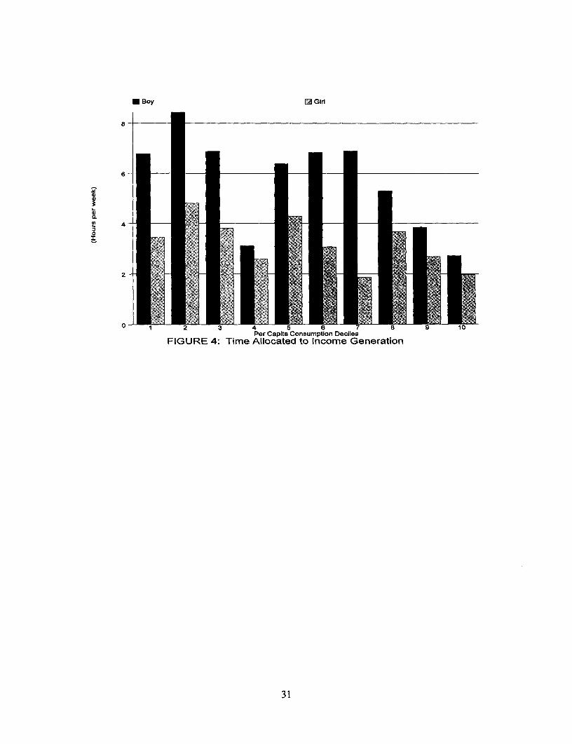
lists the time boys and girls allocate to income-generating activities. Boys spend more time on
these activities (3.7 hours per week) than do girls (2.8 hours per week). A few things are worth
noting. First the total amount of time allocated to this activity is not as high as one would expect
in a poor country like Peru. In all 23% of boys and 19% of girls engage in these activities. If I
consider only those who allocate non-zero time to income-generating activities, then the averages
are higher--16 hours per week for boys and 141/2 hours per week for girls. Figure 4 reveals a
declining trend in child labor over per capita consumption deciles. The last figure (figure 5)
provides a histogram of time allocated to non-school activities (both housework and labor) by
deciles. The reason for providing this graph is to compare the non-school work burdens of boys
and girls. Since girls work more at home and boys more outside, the question is who has a
higher work burden. Figure 5 reveals that with few exceptions, girls have a higher non-school
27 As mentioned above time allocated to school is only available for 1994. Thus an additional variablecapturing the grade-for-age attaimnent in school is also used as a dependent variable.
17

work burden than do boys. There is a declining trend of this work with per capita consumption,
and this declining trend is sharper for girls than for boys. This suggests that in poor households
the work burden of girls is high.
Summary statistics of the sample used in the estimation are presented in table 1. The
statistics are differentiated by gender. Here I discuss the salient differences between boys and
girls. The average grade-for-age is about 75%. Consistent with data from the rest of Latin
America, grade-for-age in our sample is higher for girls than for boys. Raw grade attainment is
however the same for both groups (about 4.5). This is not inconsistent with the grade-for-age
differences between the two sexes, as the girls in the sample are slightly younger than boys. As
far as time allocated to school is concerned, about 22-23 hours in the week prior to the survey
were allocated to schooling.29 There is no difference in the average time spent in school between
boys and girls. The summary statistics on educational activities and attainment in the data reveal
that there is little difference between boys and girls. However, what is of interest from the
perspective of this paper is whether the lack of difference in education attainment by gender that
regularly emerges from data in Latin America is also reflected in an econometric estimation of
the determinants of time allocation to various activities by gender.
Summary statistics for the other explanatory variables reveal the following. About 9%
of the children in the sample belong to female-headed households. About 15% of the children
are of native origin. About 39% belong to households that use firewood or coal for their energy
needs. One-fiflh of the children are in households that get their water from outside the premises
of the household. One in five children are also in households where a child had been sick in the
30 days prior to the survey. 39% of the children are in households where an adult had been sick
28 A grade-for-age of 100 means complete attainment, while grade-for-age equal to zero means noeducation after age 6.29 As was mentioned earlier, there is a tendency on the part of majority of school-going respondents toreport 25 hours per week in this activity.
18

during the same time period. Last, about 40% of the children in the sample are in rural
households.
IV. Empirical Results
Schooling
Results of estimation of the determinants of schooling attainment (grade-for-age) and time
allocated to school (full-time or not) by gender are given in table 2. The grade-for-age
regressions are conducted using the random effect approach. Since data on time spent in school
are only available for the 1994 subset, this regression is estimated using a simple probit. As
grade-for-age is a measure of attainment that goes beyond time allocated to schooling in the week
prior to interview, it is unlikely it will be affected by sickness, which is measured in the data over
a 30-day period prior to interview. Sickness variables are therefore not included as right hand
side variables in the grade-for-age regression.
The estimation results of the determinants of grade-for-age by gender reveal interesting
patterns. A comparison of columns 1 (girls) and 2 (boys) reveals that age, birth order, household
demographics (female headship, age structure and size), household access to basic services
(energy and water) and household wealth significantly affect the grade-for-age of girls but not of
boys. For girls, grade-for-age drops with age whereas it is not statistically different from zero for
boys. Female headship also significantly lowers the attainment of girls but not of boys. As
household wealth increases, grade-for-age of girls improves significantly whereas that for boys
stays unchanged. The presence of prime-age females in the household (those between 16 and 60)
affects the educational attainment of girls by a large magnitude but it has no effect on the
attainment of boys. This suggests that there is a substitution between the time of young girls and
adult females in the household, and that this effect works through housework (table 3). As
household size increases (another indicator of poverty) the attainment of girls falls at a
19
statistically significant rate. There is no effect of household size on the attainment of boys. In
rural areas, sibling rank significantly affects the attainment of girls but not of boys. The
education of the oldest prime-age female in the household significantly increases the grade-for-
age for both boys and girls.
While grade-for-age measures educational attainment over a long period, it is only an
indirect measure of the stock of time use. A closer measure of time use is the time children
allocate to school. Since this information is not available for 1997, I present the results of probit
regression on decision to attend school full-time based on cross section (1994 panel households
only) in columns 3 and 4. Here the decision to attend school full-time is positively associated
with age-it increases with age but at a decreasing rate. The estimated coefficients of other
regressors are largely insignificant, suggesting that unobserved heterogeneity may be clouding
the estimated standard errors. I therefore do not discuss these results in detail here but provide
them for illustrative purposes only.
Housework
Estimation results of the determinants of time allocation to housework are presented in table 3.
Here, there are some effects that are common to boys and girls, and some that are stronger for
girls than for boys. Among the common effects, age increases the housework time of both boys
and girls but at a decreasing rate. Household size and the age structure of females in the
household also affect boy-girl time in housework in a similar manner. Children in bigger
households tend to do less housework, presumably because of economies of scale in housework.
The presence o:f prime-age females in the household lowers the housework time of both boys and
girls. Birth order significantly increases the time allocation to housework for both boys and girls,
suggesting that older siblings engage more in housework than do younger ones. Changes in
cluster level female unemployment also affect the housework time of both boys and girls. In
20

urban areas, increases in female unemployment significantly lower the housework time of both
boys and girls, though the effect is stronger in magnitude for girls. This finding, combined with
that on the effect of presence of prime-age females on housework and schooling, points to the
presence of substitution of housework time between adult women and young children. When
women do not participate in the labor market, the time urban children have to spend in household
chores tends to be lower than if they do. This effect is opposite for the rural sample, although it
is much lower in magnitude and insignificant for boys. This result is also consistent with the
findings in Grootaert and Patrinos (1999).
The results for housework differ by gender for a number of explanatory variables. First,
native status increases housework time of urban girls relative to non-native ones. However, there
is no effect on housework time of native boys relative to non-native ones. As was the case for
schooling, household wealth lowers the time on housework of girls and has no effect on that of
boys. Urban girls spend a lot more time on housework than do their rural counterparts.
However, there are no differences between rural and urban boys. Lastly, the burden of sickness
in the household also affects the time use of children.30 The sickness of a young child forces
young girls to allocate more time to housework (tending the sick). There is no statistically
significant effect on housework done by boys.
Child labor
Table 4 presents the results of the determinants to the decision of boys and girls to work in
income-generating activities. The equations are estimated using a random effect probit
specification. Recall from table I that only 19% of girls and 23% of boys engage in such
activities. The results indicate that age influences the propensity to engage in child labor, but at
a decreasing rate. After controlling for age, birth order influences the decision to work of boys
21

but not of girls. The higher the sibling rank of a boy, the more likely he is to work. The same is
not true for girls--lower sibling rank girls are as likely to work as higher ones. There is an
interesting effect of female headship of household on child labor. In rural areas, female headship
results in lower child labor among boys but no difference for girls. Similarly, the education of
the oldest prime-age female in the household tends to have a beneficial effect on the child labor
of boys but not girls. In rural areas, household wealth is negatively associated with the child
labor decision of girls but not of boys. Thus as households get richer, there is a positive effect on
the time use of girls, but not of boys. Interestingly, the age composition of the household does
not affect the propensity of either boys or girls to work. However, the size of the household does
tend to lower child labor. As household size increases, the propensity for work of children falls,
with the effect for boys being statistically significant at the 5% level. This result is counter to
what one would expect given that larger households also tend to be poorer in Peru (World Bank,
1998). Neither the presence of prime-age females in the household nor female unemployment
rates at the cluster level have any effect on child labor. Household access to water services has a
significantly negative effect on child labor in urban areas. This suggests that there may be
complementarities between work and obtaining water. No such effect appears in the rural areas.
The results for the effect of sickness and disease of children and adults on child labor are also
interesting. In rural areas, the sickness of a child in the household forces girls to withdraw from
work (presumably to take care of the sick) with no effect on boys. On the other hand, the
presence of a sick adult in the household forces girls into child labor more than it does boys.
Both these results suggest that young girls in rural Peru may be particularly vulnerable to
sickness in the household.
V. Policy Lessons
30 Recall in this paper sickness is considered endogenous at the household level. Instrunents of sickness
22

This paper investigates the determinants of time use of boys and girls in Peru. It argues for the
inclusion of housework in the broader definition of child labor. By not doing so, one runs the
risk of overlooking the effects of important factors such as household welfare, age composition,
adult employment and sickness on children's time use, particularly that of girls. In order to
improve schooling outcomes of both sexes, policymakers need to be aware of household factors
that can also constrain the demand for schooling. The traditional approach of defining the debate
on child labor by focusing on the choice between income-generating activities and schooling is
likely to have a gender-bias since girls tend to work primarily at home and boys outside.
This paper also finds that while overall educational attainment may not be very different
between boys and girls, the demand for girls schooling and their labor activities responds more
strongly to household welfare, demographics and adult female employment than does that of
boys. Safety nets that protect household incomes from employment shocks and sickness and
childcare programs that allow adult women to work would therefore make it less likely that girls
would be pulled out of school.
are therefore used in the regression here.
23

VI. References
Basu, Kaushik, 1998, "Child Labor: Cause, Consequence and Cure, with Remarks onInternational Labor Standards," Department of Economics, Cornell University,mimeograph.
Canagarajah, R. Sudarshan and Harold Coulombe, 1998, "Child Labor and Schooling in Ghana,"Working Paper Series, no. 1844, The World Bank, Washington DC.
DeGraff, D. S., R. E. Billsborrow and A. N. Herrin, 1993, "The implications of high fertility forchildren's time use in the Philippines," in Lloyd (ed.).
Durryea, Suzarne, 1999, "Children's Advancement through School: The Role of TransitoryShocks to Household Income," Working Paper #376, Inter-American Development Bank:Washington DC.
Fafchamps, Marcel and Agnes R. Quisumbing, 1998, "Social Roles, Human Capital and the Intrahousehold Division of Labor: Evidence from Pakistan," Department of Economics,Stanford University. Mimeograph.
Greene, William, 1997, Econometric Analysis, Prentice Hall: New Jersey. 3rd Edition.
Gronau, Reuben, 1977, "Leisure, Home Production and Work -- The Theory of the Allocation ofTime Revisited," Journal of Political Economy, 85, 1099-1123.
Grootaert, Christian and Harry A. Patrinos, 1999, Policy Analysis of Child Labor: AComparative Study, St. Martin's Press (forthcoming).
Grootaert, Christian and Ravi Kanbur, 1995, "Child Labor," Policy Research Working Paper1454, The World Bank, Washington DC.
Ilahi, Nadeern and Saqib Jafarey, 1998, "Markets, Deforestation and Female Time Allocation inRural Pakistan," Department of Economics, McGill University. Mimeograph.
Jensen, Peter and Helena S. Nielsen, "Child labour or school attendance? Evidence fromZambia," Journal of Population Economics, 10, 407-424.
Jacoby, Hanan and Emmanuel Skoufias, 1997, "Risk, Financial Markets and Human Capital in aDeveloping Country," Review of Economic Studies, 64, 311-335.
Kevane, Michael and Bruce Wydick, 1998, "Social Norms and the Time allocation of Women'sLabcr in Burkina Faso," Economics Department, University of Santa Clara, mimeograph.
Kumar, Shubh K. and D. Hotchkiss., 1988, "Consequences of Deforestation for Women's TimeAllocation, Agricultural Production, and Nutrition in Hill Areas of Nepal," ResearchReport 69, International Food Policy Research Institute: Washington DC.
Mason, Andrew and Julian Lampietti, 1998, "Integrating Gender into Poverty Analysis:Concepts and Methods," Working Paper, The World Bank, Washington DC.
Mason, Andrew D. and Shahid R. Khandker, 1997, "Household Schooling Decisions inTanzania," The World Bank, Washington DC. mimeograph.
Patrinos, Harry A., and George Psacharopoulos, "Family Size, schooling and child labor inPent-An empirical analysis," Journal of Population Economics, 10, 387-405.
Pitt Mark M. and Mark R. Rosenzweig, 1990, "Estimating the Intrahousehold Incidence ofIllness: Child Health and Gender-Inequality in the Allocation of Time," InternationalEconomic Review, 31, 969-989.
24

Psacharopoulos, George, 1997, "Child labor versus educational attainment: Some evidence fromLatin America," Journal of Population Economics, 10, 377-386.
Rosenhouse, Sandra, 1989, "Identifying the Poor: Is 'headship' a useful concept?" LSMSWorking Paper no. 58, The World Bank, Washington DC.
Rosenzweig, Mark and Oded Stark, 1989, Consumption Smoothing, Migration and Marriage:Evidence from Rural India, Journal of Political Economy, 97, 905-926.
Skoufias, Emmanuel, 1993, "Labor Market Opportunities and Interfamily Time Allocation inRural Households in South Asia," Journal of Development Economics, 40, 277-310.
Tzannatos, Zafiris, 1995, "Economic Growth and Gender Equity in the Labor Market," Povertyand Social Policy Department, The World Bank, Washington DC.
World Bank, 1998, "Peru: Poverty Comparisons," Country Department 6, Latin America andCaribbean Region, The World Bank, Washington DC.
25

V. Appendix: The Determinants of Child and Adult Sickness
The incidence of disease is measured by a discrete variable-if an adult (or a child) were sick in
the last 30 days.3' Sickness and disease are considered as household level effects, i.e. all
individuals within a household are assumed to have the same probability of falling sick. Random
effects probit regression were run for the two types to generate instruments. The right hand side
variables are: a) cluster proportion of households with infrastructure (namely, sanitation
facilities, gas or electricity, electric lighting, running water, hours of public water supply), b)
demographic characteristics (namely, median age of household, highest level of education in
household, the number of male and female members below 15 and more than 60 years of age), c)
physical characteristics of the dwelling (namely, whether it has concrete or tile roofing and the
number of rooms per capita) and lastly dummies for rural and native status.
The results are provided in the Appendix table. Only the salient results are summarized
here. Household characteristics appear to have a strong influence on household health.
Households that are farther along in the life-cycle have a lower probability of child and adult
sickness. Bigger households tend to have more illness than smaller ones. Native households are
no more likely to have illness than their non-native counterparts. The highest level of education
completed by a household member tends to lower the incidence of child disease (thought the
effect is below significance). Surprisingly, it increases the probability of adult sickness. The
age/gender composition of the household also matters. The presence of adolescent boys and girls
significantly reduces the incidence of sickness and disease in the household. The fact that young
children provide health public goods in the household comes out quite starkly in these results.
The result for adolescent boys tends to be weaker than that for girls, and their role in influencing
31 The survey also contains information on the number of days an individual in the household was sick andthe number of days that individual was bed ridden. The results using these variables were no different thanthose with discrete indicators of sickness.
26

adult sickness is insignificant. The presence of the elderly does not appear to influence the
sickness and disease in the household, except for the effect of elderly women on adult sickness.
27

a Boy E Girl
30 - _
00
Per Capita Consumption DecilesFIGURE 1: Time Allocated to Schooling (1994 only)
28

U Boy 1 Girl
100 -
0
P er Capita Consumption DecilesFIGURE 2: Grade-for-Age in Education
2 9

* Boy UM Girl
15 -_
10
0.
00.
Per Capita Consumption DedliesFIGURE 3: Time Allocated to Housework
30
* Boy HI Girl
8-
I~~CD4)
P er Capita Consumption DecilesFIGURE 4: Time Allocated to Income Generation
31

* Boy ' Girl
20 -
15 _
P 1(0
0
5
1 2 3 4 5 6 7 8 9 10Per Capita Consumption Deciles
FIGURE 5: Time Allocated to All Non-school Activities
32
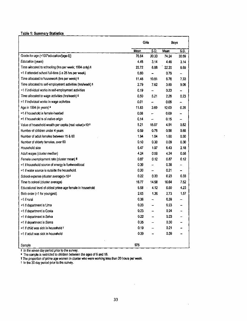
Table 1: Summary Statistics
Girls Boys
Mean S.D. Mean S.D.Grade-for-age (=100*education/[age-61) 76.64 30.33 74.24 30.59Education (years) 4.48 3.14 4.49 3.14Time allocated to schooling (hrs per week; 1994 only) 1 22.72 8.86 22.20 8.69=1 if attended school full-time (i.e 25 hrs per week) 0.80 - 0.79 -
Time allocated to housework (hrs per week) 5 11.48 10.81 6.76 7.33Time allocated to self-employment activities (hrs/week) S 2.79 7.62 3.69 9.06=1 if individual works in self-employment activities 0.19 - 0.23 -
Time allocated to wage activities (hrslweek) 1 0.50 5.21 2.26 0.23=1 if individual works in wage activities 0.01 - 0.06 -
Age in 1994 (in years) Y 11.83 3.69 12.00 0.28=1 if household is female-headed 0.08 - 0.09 -
=1 if household is of native origin 0.14 - 0.15 -
Value of household wealth per capita (real value)x 10 3 5.21 15.07 4.91 0.82
Number of children under 4 years 0.59 0.76 0.58 0.86Number of adult females between 15 & 60 1.94 1.04 1.60 0.30Number of elderly females, over 60 0.10 0.30 0.09 0.30Household size 6.47 1.97 6.43 2.18Adult wages (cluster median) 4.24 0.59 4.24 0.58Female unemployment rate (cluster mean) 1 0.87 0.12 0.87 0.12=1 if household source of energy is fuelwood/coal 0.39 - 0.38 -
=1 if water source is outside the household. 0.20 - 0.21 -
School expense (cluster average)xl0-3 0.22 0.33 0.23 0.33
Time to school (cluster average) 16.77 14.58 16.64 7.52Educational level of oldest prime age female in household 5.58 4.12 5.50 4.23Birth order (=1 for youngest) 2.65 1.36 2.73 1.57=1 if rural 0.38 - 0.39 -
=1 if department is Uma 0.20 - 0.23 -
=1 if department is Costa 0.23 - 0.24 -
=1 if department is Selva 0.22 - 0.23 -
=1 if department is Sierra 0.35 - 0.30 -
=1 if child was sick in household t 0.19 - 0.21 -
=1 if adult was sick in household 0.39 - 0.39 -
Sample 975S In the seven day period prior to the survey.M The sample is restricted to children between the ages of 6 and 18.r The proportion of prime age women in cluster who were working less than 20 hours per week.t In the 30 day period prior to the survey.
33

Table 2: The Determinants of School Attainment (grade-for-age) and Time Allocated to School by gender in Peru,1994 and 1997a
Grade-for-age b Aftending school full timec
Girls Boys(1) (2) (3) (4)
coeff t-ratio Coeff t-ratio coeff t-ratio Coeff t-ratioAge -1.311 -3.29 -0.341 -0.96 0.641 3.92 0.509 3.60
Square of age -0.031' -4.50 -0.025- -4.28
Female-headed household -8.887" -2.03 -1.068 -0.25 -0.243 -0.85 0.330 0.98
Rural x female-headed household 9.484 0.95 -9.124 -0.94 -0.708 -0.95 -0.724 -1.19Native -6.610 -0.85 -4.703 -0.58 -0.474 -1.04 -0.164 -0.32Rural x native 6.019 0.69 -4.334 -0.49 1.013 1.77 -0.081 -0.14Wealth per capita (log) 1.967" 2.08 1.017 1.04 -0.267 -0.34 -0.049 -0.62
Rural x wealth per capita 0.967 0.62 -0.094 -0.06 0.083 0.70 -0.013 -0.12# of children under 4 years -1.521 -0.87 -2.016 -1.26 0.317 2.17 -0.059 -0.48
#of adultfemales between 15&60 5.198 .4.01 0.761 0.52 -0.125 -1.16 -0.069 -0.65
#ofelderlyfemales, over60 0.544 0.15 1.757 0.49 -0.107 -0.36 -0.033 -0.13Household size -2.332" -2.73 -0.717 -0.83 0.119 1.60 -0.069 -1.10
Adult wage (cluster median; log) -2.565 -1.05 -0.607 -0.26 0.376 1.59 0.324 1.46Female unemployment rate -9.685 -0.92 -2.029 -0.20 0.461 0.49 1.031 1.23Rural x female unemployment rate 28.532 1.28 1.160 0.05 -5.256 -2.24 -2.515 -1.21Household energy: fuelwood/coal -2.414 -0.57 -11.166" -2.37 -1.087" -3.47 -0.565 -1.82
Rural x household energy: luelwood/coal -9.992' -1.67 -2.869 -0.44 2.132 4.05 0.642 1.40
Water source: outside. -16.895" -2.71 -5.318 -0.86 -0.227 -0.55 -0.777 -2.18
Rural x water source outside 22.058" 3.07 11.388 1.60 0.878 1.66 0.196 0.42School expenses (cluster average) -0.003 -0.97 -0.005 -1.10 0.001 0.59 0.002 1.19Time to school (cluster average) 0.173" 2.52 -0.013 -0.08 -0.037 -1.88 -0.008 -0.42
Rural x time to school -0.405' -1.89 0.147 0.56 0.065 2.37 0.018 0.66Educational of oldest prime age female 0.793" 2.31 0.833" 2.31 -0.008 -0.31 -0.034 -1.29
Rural x highest education iI household -0.014 -0.02 -0.484 4.71 0.021 0.34 0.050 0.93Birth order (=1 for youngest) 0.370 0.26 0.038 0.03 -0.206 -1.90 0.050 0.54
Rural x birth order 3.098 1.82 0.776 0.53 -0.065 -0.44 0.100 1.02Rural -38.269 -1.47 -3.612 -0.14 1.842 0.69 1.707 0.71
NWald statistic (X2with 24 d.f)
p (= alcx+ ad)R2(within)R2 (between)
R2 (overall)a The sample consists of children aged 6-18 in panel households only, The regressions also included an intercept and dummies for regions (Lima,
Costa and Selva).b Random-effects regression. Dependent variable is grade-for-age (=100*education/[age-61). The regression also included a time dummy.c Probit regression on 1994 panel individuals only. Dependent variable =1 if time in school in past week was no less than 25 hours and =0
otherwise.Statistically significant at the 5% level. - Statistically significant at the 10% level.
34

Table 3: The Determinants of Time Allocated to House ork by Gender in Peru, 1994 and 1997 a
Girls Boys(1) (2)
coeff t-ratio coeff t-ratio
Age 0.335" 5.39 0.408 6.23Square of age -0.008- -3.37 -0.015 -5.49Female-headed household 0.067 0.46 0.123 0.90Rural x female-headed household 0.091 0.27 0.153 0.51Native 0.463 1.86 0.324 1.28Rural x native -0,581" -2.07 -0.287 -1.03Wealth per capita (log) -0.091" -2.66 -0,018 -0.50Rural x wealth per capita 0.127" 2.32 -0.031 -0.57# of children under 4 years 0.023 0.34 0.005 0.08# of adult females between 15 & 60 -0.124" -2.58 -0.139 -2.67# of elderly females, over 60 -0.101 -0.79 -0.220 -1.67Household size -0.143" -4.26 -0.116 -3.62Adult wage (cluster median; log) -0.076 -0.89 0,008 0.10Female unemployment rate -1.607 -4.39 -0.969 -2.54Rural x female unemployment rate 1.938" 2.57 0.399 0.47Household energy: fuelwood/coal -0.160 -1.10 0.269 1.66Rural x household energy: fuelwood/coal 0.275 1.35 0.085 0.39Water source: outside. 0.208 1.00 -0.197 -0.99Rural x water source outside -0.488" -1.96 0,259 1.07School expenses (cluster average) )x1 0-3 -0.129 -1.01 0,068 0.49Time to school (cluster average) 0.002 0.67 -0.008 -1.17Rural x time to school 0.002 0.34 0,003 0.33Educational of oldest prime age female -0.005 -0.40 -0,011 -0.89Rural x highest education in household -0.025 -1.04 0.017 0.75Birth order (=1 for youngest) 0.128" 2.58 0.090 1.89Rural x birth order -0.131" -2.14 -0.030 -0.56Rural -2.164" -2.49 -0.410 -0.43Child sick b 0.420" 2.42 0.304 1.62Rural x child sick 0.133 0,57 0.127 0.53Adult sick b -0.021 -0.10 0.125 0.57Rural x adult sick -0.201 -1.59 -0.219 -1.55
NWald statistic (X2 with 24 d.f.)
p (=a la+ a1)R2 (within)R2 (between)
R2 (overall)a Random-effects regression. The sample consists of children aged 6-18 in panel households only. The regressions also included an intercept
term, dummies for regions (Lima, Costa, Selva) and a time dummy.b Both child and adult sickness are considered endogenous. See the appendix for details.
Statistically significant at the 5% level. Statistically significant at the 10% level.
35

Table 4: The Determinants of Child Labor Decision by Gender in Peru, 1994 and 1997 8
Girls Boys(1) (2)
Coeff t-ratio Coeff t-ratioAge 0.373 3.04 0.498 4.13Square of age -0.013- -2.47 -0.016 -3.387Female-headed household 0.180 0.67 -0.181 -0.65Rural x female-headed household -0.510 -0.95 -0.850 -1.68Native 0.292 0.71 0.397 1.00Rural x native 0.203 0.45 0.451 1.06Wealth per capita (log) 0.057 0.80 -0.006 -0.09Rural x wealth per capita -0.208 -2.18 0.117 1.26# of children under 4 years 0.183 1.57 0.166 1.52# of adult females between 15 & 60 0.024 0.27 0.025 0.27# of eldedy females, over 60 0.171 0.72 -0.183 -0.73Household size -0.040 -0.65 -0.116 -1 .97Adult wage (cluster median; log) -0.204 -1.34 -0.011 -0.08Female unemployment rate 0.470 0.56 1.181 1.37Rural x female unemployment rate -0.206 -0.16 -0.025 -0.02Household energy: fuelwood/coal -0.180 -0.70 -0.409 -1.41Rural x household energy: fuelwood/coal 0.214 0.64 0.459 1.31Water source: outside. 0.585 1.78 0.584 1.92
Rural x water source outside -0.633 -1.65 -0.543 -1.52School expenses (duster average) )x1O-3 -0.188 -0.44 0.075 0.19Time to school (cluster average) -0.001 -0.09 -0.022 -1.23Rural x time to school -0.017 -1.46 0.022 1.11Educational of oldest prme age female -0.018 -0.74 -0.057 -2.29Rural x highest education in household -0.063 -1.63 0.044 1.19Birth order (=1 for youngest) 0.140 1.54 0.165 1.80
Rural x birth order -0.108 -1.09 -0.123 -1.33Rural 2.669 1.80 -0.195 -0.13
Child sick b -0.108 -0.31 -0.023 -0.06Rural x child sick -1.233 -3.08 0.076 0.19Adult sickb 0.511 1.21 0.241 0.62Rural x adult sick 0.534 2.13 -0.066 -0.27
NWald statistic (e with 24 df)
p (0c4au+aj)R2 (within)R2(between)R2 (overall)
a Random-effects probit iegression. Dependent variable is =1 if child worked in income generating activities and =0 otherwise. The sampleconsists of children aged 6-18 in panel households only. The regressions also included an intercept, dummies for regions (Uma, Costa, Selva)and a time dummy.
b Both child and adult sickness are considered endogenous. See the appendix for details.Statistically significant at the 5% level. Statistically significant at the 10% level.
36

Appendix Table: The Determinants of Child and Adult Sickness in Peru, 1994 and 1997
Child Sickness Adult Sickness
Median household age -0.015 -0.005(-4.22) (-2.33)
Native -0.118 -0.071(-0.87) (-0.71)
Maximum education in household -0.017 0.023(-1.27) (2.35)
Hours of public water supply in cluster -0.000 -0.004(-0.05) (-0.87)
% of households in cluster with sanitation -0.252 0.068(-1.28) (0.44)
% of households in cluster with gas/electricity 0.233 -0.304(1.21) (-2.13)
% of households in cluster with in-house water 0.007 0.385(0.04) (2.71)
% of households in cluster with electric lighting 0.142 0.261(0.85) (1.95)
Roof: concrete -0.106 -0.004(-0.95) (-0.05)
Roof: wood -0.115 -0.351(-0.48) (-1.91)
Roof: tiles -0.168 0.010(-1.36) (0.10)
Rooms per capita -0.299 -0.101(-2.38) (-1.82)
Household size 0.207 0.069(7.80) (3.20)
Number of boys in household (5-14) -0.027 -0.010(-352) (-1.56)
Number of girls in household (5-14) -0,028 -0.023(-3.69) (-3.45)
Number of elderly men in household (>60) -0.021 -0.001(-1.02) (-0.08)
Number of elderly women in household (>60) 0.019 -0.031(0.87) (-1.76)
Rural 0.245 0.273(1.46) (2.11)
Constant -1.154 -1.000(-4.38) (-4.94)
Number of households 898 898Number of observations per household 2 2x2(18) 156.87 96.19
a Random-effects probit regression. Dependent varlables are, respectively, child and adult sickness dummies. t-ratios are given in parenthesesbelow coefficient estimates.
37


Policy Research Working Paper Series
ContactTitle Author Date for paper
WPS2730 Antidumping as Safeguard Policy J. Michael Finger December 2001 R. SimmsFrancis Ng 37156Sonam Wangchuk
WPS2731 An Alternative Technical Education Gladys Lopez-Acevedo December 2001 M. GellerSystem in Mexico: A Reassessment 85155of CONALEP
WPS2732 The Unbalanced Uruguay Round J. Michael Finger December 2001 R. SimmsOutcome: The New Areas in Future Julio J. Nogues 37156WTO Negotiations
WPS2733 Trade Policy Reform and Poverty Bernard Hoekman December 2001 R. MartinAlleviation Constantine Michalopoulos 39065
Maurice SchiffDavid Tarr
WPS2734 Agricultural Markets in Benin and Marcel Fafchamps December 2001 P. KokilaMalawi: The Operation and Eleni Gabre-Madhin 33716Performance of Traders
WPS2735 Shifting Tax Burdens through Bernard Gauthier December 2001 H. SladovichExemptions and Evasion: An Empirical Ritva Reinikka 37698Investigation of Uganda
WPS2736 Social Policy and Macroeconomics: F. Desmond McCarthy December 2001 J. TurnerThe Irish Experience 81767
WPS2737 Mode of Foreign Entry, Technology Aaditya Mattoo December 2001 R. MartinTransfer, and Foreign Direct Marcelo Olarreaga 39065Investment Policy Kamal Saggi
WPS2738 Assisting the Transition from Emanuela Galasso December 2001 C. CunananWorkfare to Work: A Randomized Martin Ravallion 32301Experiment Agustin Salvia
WPS2739 Poverty, Education, and Health in Peter Lanjouw December 2001 P. SaderIndonesia: Who Benefits from Public Menno Pradhan 33902Spending? Fadia Saadah
Haneen SayedRobert Sparrow
WPS2740 Are Men Benefiting from the New Omar Arias December 2001 S. NyairoEconomy? Male Economic 34635Marginalization in Argentina, Brazil,and Costa Rica

Policy Research Working Paper Series
ContactTitle Author Date for paper
WPS2741 Female Wage Inequality in Latin Luz A. Saavedra December 2001 S. NyairoAmerican Labor Markets 34635
WPS2742 Sectoral Allocation by Gender of Wendy V. Cunningham December 2001 S. NyairoLatin American Workers over the 34635Liberalization Period of the 1960s
WPS2743 Breadwinner or Caregiver? How Wendy V. Cunningham December 2001 S. NyairoHousehold Role Affects Labor 34635Choices in Mexico
WPS2744 Gender and the Allocation of Nadeem llahi December 2001 S. NyairoAdult Time: Evidence from the Peru 34635LSMS Panel Data