Embed Size (px)
Citation preview
Child and Working-Age Poverty from 2010 to 2020 IFS Commentary C121 Mike Brewer James Browne Robert Joyce

Child and working-age poverty from 2010 to 2020
Mike Brewer
James Browne
Robert Joyce
Institute for Fiscal Studies
Copy-edited by Judith Payne
The Institute for Fiscal Studies 7 Ridgmount Street London WC1E 7AE

Published by
The Institute for Fiscal Studies 7 Ridgmount Street London WC1E 7AE
Tel: +44 (0)20 7291 4800 Fax: +44 (0)20 7323 4780 Email: [email protected]
Website: http://www.ifs.org.uk
Printed by
Pureprint Group, Uckfield
© The Institute for Fiscal Studies, October 2011
ISBN: 978-1-903274-86-6

Preface
The Joseph Rowntree Foundation has supported this project as part of its programme of research and innovative development projects, which it hopes will be of value to policymakers, practitioners and service users. The facts presented and views expressed in this Commentary are, however, those of the authors and not necessarily those of the Foundation, nor of the other individuals or institutions mentioned here, including the Institute for Fiscal Studies, which has no corporate view. The authors acknowledge the contribution made by Joel Banford, Rafal Chomik, Carl Emmerson, Saranna Fordyce, Chris Goulden, Paul Gregg, Gawain Heckley, Donald Hirsch, Anne MacDonald, Patrick Nolan, Stefania Porcu, Holly Sutherland and Graham Whitham, who provided advice during the project or comments on earlier drafts. We are extremely grateful to Amy Morgan for her advice on how to model Universal Credit. The Family Resources Survey is crown copyright material and is reproduced with the permission of the Controller of HMSO and the Queen’s Printer for Scotland. It was obtained from the Economic and Social Data Service at the UK Data Archive.
James Browne and Robert Joyce are at the Institute for Fiscal Studies and Professor Mike Brewer is at the Institute for Social and Economic Research at the University of Essex.
Correspondence to: [email protected].

Contents
Extended summary 1
1.
Introduction 5
2. Child poverty: past performance and policy context for the future 6 2.1 Child poverty under the Labour government 6
2.2 Child poverty over the next decade 8
3. Results 10 3.1 The path of poverty to 2013 under current policies 10 3.2 The effect of Universal Credit in 2014 and 2015 13 3.3 Projections of poverty in 2020 under different scenarios 18
3.4 The direct impact on poverty of the coalition government’s tax and benefit reforms
23
4.
Sensitivities 28
5.
Conclusion 31
Appendices 33 Appendix A. Details of assumptions and modelling procedures 33 Appendix B. Poverty projections under full take-up and without applying
any ‘correction’ to simulated incomes 51
Appendix C. Poverty projections without the coalition government’s tax and benefit reforms
53
Appendix D. Poverty rates using 50% and 70% of median income 55
References 59


1
© Institute for Fiscal Studies, 2011
Extended summary
This Commentary presents forecasts of relative and absolute income poverty in the UK among children and working-age adults for each year between 2010---11 and 2015---16, and for 2020---21, using a static microsimulation model augmented with forecasts of key economic and demographic characteristics. It updates and extends previous JRF-funded work by Mike Brewer and Robert Joyce, which forecast poverty through to 2013---14, and builds on previous ESRC-funded work by Mike Brewer, James Browne and Wenchao Jin, which simulated the impact of Universal Credit on household incomes.
This exercise is necessarily subject to uncertainties and limitations. Macroeconomic forecasts such as those we make use of here are always highly uncertain, and this is especially true at present; the data available do not enable us to model all of the tax and benefit changes coming in over the next few years precisely, and we cannot fully account for the impacts of behavioural changes that result from tax and benefit reforms; and the underlying survey data used are, of course, subject to sampling error. However, the results should provide a useful guide to what might happen to poverty under current government policies.
Background
The Child Poverty Act, passed with all-party support in 2010, commits successive governments to the eradication of child poverty by 2020. The Act lists four measures of child poverty, each with their own target which needs to be met for child poverty to be said to be eradicated, but this Commentary concentrates on relative and absolute poverty, as the other measures cannot yet be modelled. The Act defines an individual to be in relative poverty if his or her household’s equivalised income is below 60% of the median in that year; and he or she is in absolute poverty if the household’s equivalised income is below 60% of the 2010---11 median income, adjusted for inflation. All numbers referred to in this Extended Summary are for poverty with incomes measured before housing costs have been deducted; conclusions are very similar for poverty with incomes measured after housing costs have been deducted.
Incomes and poverty under current policies
The table on the next page gives the central forecasts of relative and absolute poverty amongst children and working-age adults in every year between 2010---11 and 2015---16, and in 2020---21, as well as actual poverty in 2009---10.
In the short run, relative child poverty is forecast to remain broadly constant between 2009---10 and 2012---13, before rising slightly in 2013---14. Relative working-age adult poverty is forecast to rise slightly between 2009---10 and 2012---13, before rising faster in 2013---14. Absolute child and working-age adult poverty are forecast to rise continuously, and by more than relative poverty, over this period. This unusual pattern arises because the living standards of low-income families are set to fall over the period --- which will increase absolute poverty --- but they are forecast to fall by less than the living standards of families at median income, and so relative poverty is forecast to have fallen in 2010---11. Indeed, at its low point, real median household income is forecast to be 7% lower in 2012---13 than it was in 2009---10, and to remain below its 2009---10 level until at least 2015---16. This unprecedented collapse in living standards is chiefly due to the (actual or forecast) high inflation and weak earnings growth over this period. As families in poverty get much of their income from state benefits and tax credits, which are typically increased in line with inflation, a fall in real earnings closes the gap between them and families around median income, who get much of their income from earnings.

Child and working-age poverty from 2010 to 2020
2
© Institute for Fiscal Studies, 2011
The previous Labour government had set itself targets for relative child poverty to fall by a quarter of its 1998---99 level by 2004---05, and by a half by 2010---11. Child poverty in 2010---11 is forecast to be considerably higher than the target level, falling by just over a quarter in 12 years, rather than by a half.
Between 2013---14 and 2015---16, absolute poverty is forecast to fall slightly, and relative poverty to rise slightly as real earnings return to positive growth. Between 2015---16 and 2020---21, all measures of poverty rise or remain broadly unchanged. These central forecasts imply that relative child poverty will rise from its current level of 20% to reach 24% in 2020---21, and that child poverty against the fixed 2010---11 poverty line will reach 23% in 2020---21. These are both considerably higher than the targets specified in the Child Poverty Act (of 10% and 5% respectively), and the rate of relative child poverty forecast for 2020---21 would be the highest since 1999---2000.
Children Working-age parents Working-age adults without children
Millions % Millions % Millions %
Relative poverty
2009 (actual)
2.6 19.7 2.3 17.1 3.4 15.0
2010 2.5 19.3 2.1 16.6 3.5 15.0
2011 2.5 19.2 2.2 16.7 3.6 15.1
2012 2.6 19.6 2.2 17.0 3.7 15.1
2013 2.8 21.6 2.4 18.3 3.8 15.5
2014 2.9 22.0 2.4 18.5 3.8 15.3
2015 2.9 22.2 2.4 18.5 4.0 15.9
2020 3.3 24.4 2.6 20.0 4.9 17.5
Absolute poverty
2009 (actual)
2.2 17.0 2.0 14.9 3.1 13.6
2010 2.5 19.3 2.1 16.6 3.5 15.0
2011 2.8 21.1 2.4 18.1 3.7 15.7
2012 2.8 21.8 2.4 18.7 3.9 16.0
2013 3.1 23.2 2.5 19.5 4.0 16.3
2014 3.0 22.9 2.5 19.2 4.0 16.0
2015 3.0 22.8 2.5 19.0 4.1 16.0
2020 3.1 23.1 2.5 19.0 4.7 16.8
Notes: Poverty line is 60% of median before-housing-costs (BHC) income. Years refer to financial years. Source: Authors’ calculations based on Family Resources Survey, 2008---09, using TAXBEN and assumptions specified in the text.

Extended summary
3
© Institute for Fiscal Studies, 2011
The impact of the current government’s reforms on poverty
This Commentary estimates the impact on poverty of the coalition government’s reforms by comparing these central forecasts --- which account for government policy towards personal tax and state benefits announced as of Summer 2011 --- and a forecast that assumes that none of the reforms announced by the current government is introduced. These reforms include Universal Credit and other changes announced but not yet implemented. The comparison suggests that the impact of changes to personal tax and benefit policy announced by this coalition government is to increase relative child poverty by 200,000 in both 2015---16 and 2020---21, and to increase relative poverty for working-age adults by 200,000 in 2015---16 and 400,000 in 2020---21. The reforms are forecast to increase absolute child poverty by 200,000 in 2015---16 and 300,000 in 2020---21, and to increase absolute working-age poverty by 300,000 in 2015---16 and 700,000 in 2020---21.
The most significant reform to state benefits proposed by the government is to replace all means-tested benefits and tax credits for those of working age with a single, integrated benefit to be known as Universal Credit. Considered in isolation, Universal Credit should reduce relative poverty significantly (by 450,000 children and 600,000 working-age adults), but this reduction is more than offset by the poverty-increasing impact of the government’s other changes to personal taxes and state benefits. The most important of these other changes for poverty in 2020---21 is that benefits, including the Local Housing Allowance from April 2013, will now be indexed in line with the consumer price index (CPI) measure of inflation, rather than one derived from the retail price index (RPI).
Sensitivities
Alternative scenarios in which employment rates rise or benefit non-take-up rates fall relative to the central scenario --- perhaps due to Universal Credit --- show rates of poverty in 2020---21 which are little different from the central forecast. Variants where future earnings growth favours high or low earners also result in little difference in poverty rates, in part because of the imperfect match between individuals who are not working, or individuals who have low hourly wages, and individuals in poverty.
Implications for policy
This Commentary forecasts what might happen to poverty under current government policies and shows that governments cannot rely on higher employment and earnings to reduce relative measures of poverty. The results therefore suggest that there can be almost no chance of eradicating child poverty --- as defined in the Child Poverty Act --- on current government policy. Although this project did not assess what policies would be required in order for child poverty to be eradicated, it is impossible to see how relative child poverty could fall by so much in the next 10 years without changes to the labour market and welfare policy, and an increase in the amount of redistribution performed by the tax and benefit system, both to an extent never-before seen in the UK. IFS researchers have always argued that the targets set in the Child Poverty Act were extremely challenging, and the findings here confirm that view. It now seems almost incredible that the targets could be met, yet the government confirmed its commitment to them earlier this year, in its first Child Poverty Strategy, and remains legally-bound to hit them. We suggest the government consider whether it would be more productive to set itself realistic targets for child poverty and provide concrete suggestions for how they might be hit --- ideally, verified with a quantitative modelling exercise such as this one.
Child and working-age poverty from 2010 to 2020
4
© Institute for Fiscal Studies, 2011
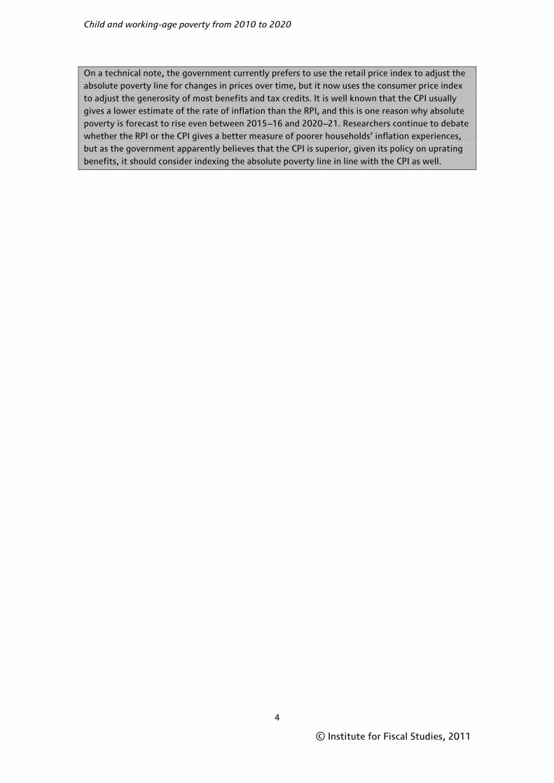
On a technical note, the government currently prefers to use the retail price index to adjust the absolute poverty line for changes in prices over time, but it now uses the consumer price index to adjust the generosity of most benefits and tax credits. It is well known that the CPI usually gives a lower estimate of the rate of inflation than the RPI, and this is one reason why absolute poverty is forecast to rise even between 2015---16 and 2020---21. Researchers continue to debate whether the RPI or the CPI gives a better measure of poorer households’ inflation experiences, but as the government apparently believes that the CPI is superior, given its policy on uprating benefits, it should consider indexing the absolute poverty line in line with the CPI as well.
5
© Institute for Fiscal Studies, 2011
1. Introduction
This Commentary provides projections of income poverty among children and working-age adults in the UK under current tax and benefit policies. We also estimate the direct impact on poverty of tax and benefit reforms announced by the coalition government. Joyce (2011) forecast poverty through to 2013–14, and we now extend his work to provide projections for each year between 2010–11 and 2015–16, and for 2020–21, incorporating what is known, at the time of writing, about Universal Credit.
We produce these projections using 2008–09 data on household incomes from the Family Resources Survey (FRS), the large-scale household survey from which official poverty statistics are derived; the IFS static tax and benefit microsimulation model, TAXBEN;1 and projections of demographic and macroeconomic variables.
There are several reasons why microsimulation techniques are well suited to poverty modelling. Such models allow for explicit simulation of the entire income distribution, which enables precise quantification of the effect on relative poverty of rises in the relative poverty line caused by rises in the median income; and such models enable us to estimate precisely the impact of direct tax and benefit changes (including often complicated interactions between them) on household incomes. This Commentary follows Brewer, Browne and Sutherland (2006), Brewer, Browne, Joyce and Sutherland (2009) and Brewer and Joyce (2010) in applying such techniques to forecast poverty in the UK. Unlike those papers, here we project poverty among the working-age population as well as among children.2
We use two definitions of income poverty, both of which are set out in the Child Poverty Act 2010. An individual is in relative income poverty in a particular year if their household income is less than 60% of the national median household income in that year. An individual is in absolute income poverty in a particular year if their household income in that year is less than 60% of the 2010–11 national median (in real terms).3 Household incomes are measured net of taxes and inclusive of benefits and tax credits, and are equivalised using the modified OECD equivalence scale. Incomes are measured both before and after housing costs have been deducted (though note that the Child Poverty Act refers only to incomes measured before housing costs have been deducted). Full details of the methodology we use to produce our forecasts are given in Appendix A.
We proceed as follows. Chapter 2 gives a brief policy background. Chapter 3 presents the results of the modelling exercise, showing projections of poverty under current policies (Sections 3.1–3.3) and without the reforms announced by the coalition government (Section 3.4). In Chapter 4, we quantify the sensitivity of our results to employment and earnings assumptions. Chapter 5 concludes.
1 For a description of TAXBEN, see Giles and McCrae (1995). The basic structure of the model has not changed since then. 2 Our model also simulates the income of pensioners, but does so in a relatively crude way, ignoring the important ‘cohort effects’ whereby new pensioners retire with higher amounts of wealth than their predecessors. For an example of a report that does attempt to forecast pensioner poverty, see Brewer et al. (2007). 3 In recent years, the absolute poverty line has been defined as 60% of the 1998---99 national median, but the 2010 Child Poverty Act says that the absolute poverty line will be rebased in 2010---11. The absolute poverty line is uprated in line with the retail price index (excluding council tax) and with the Rossi index for before-housing-costs and after-housing-costs incomes respectively.
6
© Institute for Fiscal Studies, 2011
2. Child poverty: past performance and policy context for the future
This chapter provides an overview of trends in child poverty since the late 1990s (Section 2.1) and briefly discusses the policy context for monitoring poverty over the forthcoming decade (Section 2.2). It draws heavily upon work co-authored by the authors of this paper (Brewer, Browne, Joyce and Sibieta, 2010; Jin, Joyce, Phillips and Sibieta, 2011).
2.1 Child poverty under the Labour government
In March 1999, the Labour government announced an unprecedented target to ‘eradicate’ child poverty by 2020–21, along with interim child poverty targets for 2004–05 and 2010–11.
The first interim target was for child poverty in Britain in 2004–05 to be one-quarter lower than its 1998–99 level, using a poverty line of 60% of median household income; this was narrowly missed. The second interim target was for child poverty in the UK in 2010–11 to be one-half its 1998–99 level. Progress towards the 2010–11 target was assessed using three definitions of poverty: a relative low income indicator, an absolute low income indicator and a combined relative low income and material deprivation indicator. The relative low income indicator used a poverty line of 60% of median household before-housing-costs4 (BHC) income; the absolute low income indicator used a poverty line of 60% of the 1998–99 BHC median (in real terms); and the combined relative low income and material deprivation indicator classified children as being in poverty if their household BHC income is below 70% of the median and they are materially deprived (as determined by answers to a series of questions about what their family can afford to do).
Table 2.1 reviews progress up to 2009–10 on these measures. It shows consistent declines in child poverty across all three measures between 1998–99 and 2004–05, but a less straightforward story thereafter. In fact, the reduction in child poverty between 1997–985 and 2004–05 is by far the largest and most sustained since the comparable series began in 1961 (see Brewer et al. (2010) for more on this).
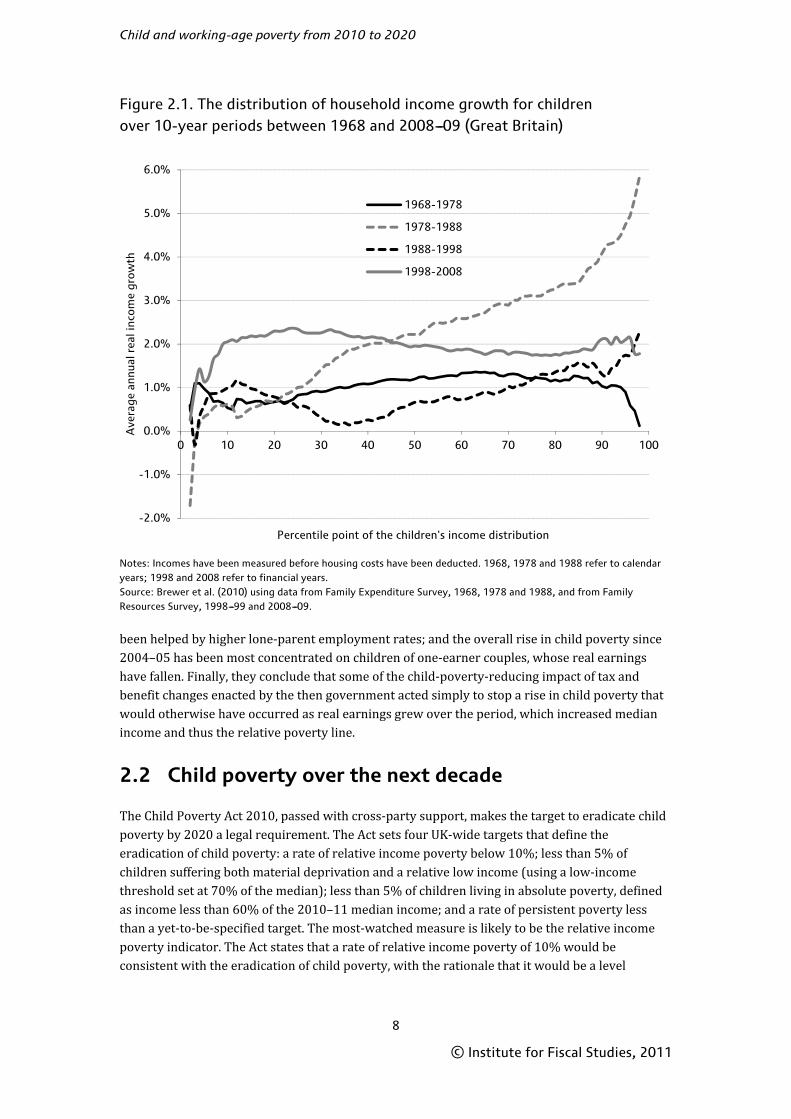
More insights on the difference between the period before and after 2004–05 are given by Figure 2.1 (from Brewer et al. (2010)), which illustrates the real average annual growth in household incomes across the children’s income distribution between 1998–99 and 2008–09, and compares this with the corresponding numbers from previous decades. Children are ordered from lowest to highest on the basis of household income and split into 100 equally sized groups, called ‘percentile groups’. The graph shows how average household income at the top of each percentile group has grown in real terms for each 10-year period between 1968 and 2008–09. In making these comparisons, it is important to realise that these periods cover different stages of various economic cycles, and income growth rates are very sensitive to this. Having noted this, Figure 2.1 shows that, between 1998–99 and 2008–09, the strongest growth in household income was
4 Incomes can be measured before or after housing costs have been deducted (BHC or AHC). Because the government’s child poverty targets related to BHC income, we focus on that in this Commentary, but we also provide figures for incomes measured AHC. 5 For consistency, we use 1998---99 as the starting point throughout this Commentary, as that is the baseline against which the child poverty targets are defined, but the downward trend in child poverty actually started between 1997---98 and 1998---99.

Child poverty: past performance and policy context for the future
7
© Institute for Fiscal Studies, 2011
Table 2.1. Progress towards halving child poverty in the UK by 2010---11
Relative poverty,UK, modified OECD (BHC)
Absolute poverty, UK, modified OECD (BHC)
Material deprivation and relative low income
% Million % Million % Million
1998---99 26.1 3.4 26.1 3.4 20.8 2.6
1999---2000 25.7 3.4 23.4 3.1
2000---01 23.4 3.1 19.1 2.5
2001---02 23.2 3.0 15.2 2.0
2002---03 22.6 2.9 14.1 1.8
2003---04 22.1 2.9 13.7 1.8
2004---05 21.3 2.7 12.9 1.7 17.1 2.2
2005---06 22.0 2.8 12.7 1.6 16.3 2.1
2006---07 22.3 2.9 13.1 1.7 15.6 2.0
2007---08 22.5 2.9 13.4 1.7 17.2 2.2
2008---09 21.8 2.8 12.4 1.6 17.1 2.2
2009---10 19.7 2.6 10.8 1.4 15.7 2.0
Change since 1998---99 ---6.3 ---0.9 ---15.3 ---2.0 ---5.1 ---0.6
Target for 2010---11 n/a 1.7
Notes: Reported changes may not equal the differences between the corresponding numbers due to rounding. The data are for the UK and incomes are equivalised using the modified OECD equivalence scale. For the purposes of the child poverty target in 2010---11, DWP has had to estimate the level of relative child poverty in the UK in 1998---99 (Northern Ireland was first included in the official HBAI series in 2002---03). For the combined indicator of material deprivation and relative low income, a threshold of 70% of median income is used to determine a relative low income. Sources: Authors’ calculations based on Family Resources Survey, various years; Department for Work and Pensions (2011). UK poverty levels for years 1998---99 to 2001---02 draw on DWP’s imputed estimates of poverty levels in Northern Ireland over this period.
found in the lower half of the children’s income distribution, approximately between the 10th and 40th percentile points. The pattern of household income growth amongst children was inequality-reducing (i.e. income growth was higher at lower points in the distribution) across a large majority of the distribution. This contrasts with previous decades (and most starkly with the decade between 1978 and 1988), when the pattern of household income growth amongst children tended to be inequality-increasing. Real household income growth amongst children over the last decade has been higher at virtually all points of the distribution than it was over the decades after 1968 and 1988. Relative to the period between 1978 and 1988, growth has been stronger across most of the bottom half of the distribution, but less strong in the top half.
Brewer et al. (2010) explore the drivers of the fall in child poverty over the past decade (and some of the reasons why child poverty did not fall as much as the government of the day would have liked). They find that direct tax and benefit reforms were very important in explaining the large overall reduction in child poverty since 1998–99, the striking slowdown in progress towards the child poverty targets between 2004–05 and 2007–08, and some of the variation in child poverty trends between different groups of children. They also find that the performance of parents in the labour market was important too: between regions, parental employment and child poverty trends are closely related; the overall reduction in child poverty since 1998–99 has
Child and working-age poverty from 2010 to 2020
8
© Institute for Fiscal Studies, 2011
Figure 2.1. The distribution of household income growth for children over 10-year periods between 1968 and 2008---09 (Great Britain)
Notes: Incomes have been measured before housing costs have been deducted. 1968, 1978 and 1988 refer to calendar years; 1998 and 2008 refer to financial years. Source: Brewer et al. (2010) using data from Family Expenditure Survey, 1968, 1978 and 1988, and from Family Resources Survey, 1998---99 and 2008---09.
been helped by higher lone-parent employment rates; and the overall rise in child poverty since 2004–05 has been most concentrated on children of one-earner couples, whose real earnings have fallen. Finally, they conclude that some of the child-poverty-reducing impact of tax and benefit changes enacted by the then government acted simply to stop a rise in child poverty that would otherwise have occurred as real earnings grew over the period, which increased median income and thus the relative poverty line.
2.2 Child poverty over the next decade
The Child Poverty Act 2010, passed with cross-party support, makes the target to eradicate child poverty by 2020 a legal requirement. The Act sets four UK-wide targets that define the eradication of child poverty: a rate of relative income poverty below 10%; less than 5% of children suffering both material deprivation and a relative low income (using a low-income threshold set at 70% of the median); less than 5% of children living in absolute poverty, defined as income less than 60% of the 2010–11 median income; and a rate of persistent poverty less than a yet-to-be-specified target. The most-watched measure is likely to be the relative income poverty indicator. The Act states that a rate of relative income poverty of 10% would be consistent with the eradication of child poverty, with the rationale that it would be a level
-2.0%
-1.0%
0.0%
1.0%
2.0%
3.0%
4.0%
5.0%
6.0%
0 10 20 30 40 50 60 70 80 90 100
Ave
rage
ann
ual r
eal i
ncom
e gr
owth
Percentile point of the children's income distribution
1968-1978
1978-1988
1988-1998
1998-2008

Child poverty: past performance and policy context for the future
9
© Institute for Fiscal Studies, 2011
comparable to the lowest in Europe (it would also be 3 percentage points lower than that achieved in the UK at any time since at least 1961).6
In previous poverty and inequality reports, IFS researchers have argued that a focus on income-based measures may skew the policy response towards reforms that have immediate and predictable impacts on household incomes – such as tax and benefit changes – rather than those that most cost-effectively improve children’s quality of life or reduce the risk of intergenerational transmission of poverty – such as improvements to education.7 To some extent, the coalition government’s Child Poverty Strategy, published on 5 April 2011, recognises this problem.8 It states that poverty is ‘about far more than income’ and expresses concern that a focus on the ‘symptoms’ as opposed to ‘causes’ of poverty led to poor policymaking and poor outcomes. Hence, as well as a new measure of income-based severe poverty, the strategy sets out a number of ancillary indicators that will be tracked to assess whether the government is on course to eradicate child poverty. These indicators are grouped into broad themes, and progress on improving them (and on meeting the existing income-based targets) is linked to a number of specific government policies (see Jin et al. (2011) for more discussion). But it is not clear whether the particular policies to be implemented will materially reduce child poverty and improve children’s life chances. And, although a focus on early educational intervention is welcome, it is highly unlikely that successful interventions could have an impact on the level of income-based child poverty as close as nine years away.
6 Reducing income poverty amongst children to zero is infeasible for at least three reasons: incomes are volatile in the short run, so there will always be some people with very low incomes at any point in time, e.g. due to self-employment losses or transition between jobs (clearly this applies less to the persistent poverty target); survey data are always subject to misreporting and the Family Resources Survey under-records benefit and tax credit receipt (see appendix C of Brewer, Muriel, Phillips and Sibieta (2008)); and the take-up rate for means-tested benefits and tax credits will never be 100%. 7 See, for example, box 4.2 of Brewer, Muriel, Phillips and Sibieta (2009). 8 HM Government, 2011.
10
© Institute for Fiscal Studies, 2011
3. Results
In this chapter, we first outline our poverty projections under current policies (Sections 3.1–3.3) and then take a look at the impact of tax and benefit reforms announced by the coalition government on these projections (Section 3.4).
When presenting poverty levels, we round to the nearest 100,000. When comparing poverty across years, or under different tax and benefit systems, we compare unrounded poverty levels and report the differences rounded to the nearest 100,000. Therefore, due to rounding, differences between rounded poverty levels shown in the tables in this chapter may not equal the differences reported in the text. This follows the convention used by the Department for Work and Pensions (DWP) in the official Households Below Average Income (HBAI) series. All years are financial years, because the Family Resources Survey (the survey of household incomes on which official poverty statistics are based) covers financial years; thus ‘2009’ refers to 2009–10 etc.
3.1 The path of poverty to 2013 under current policies
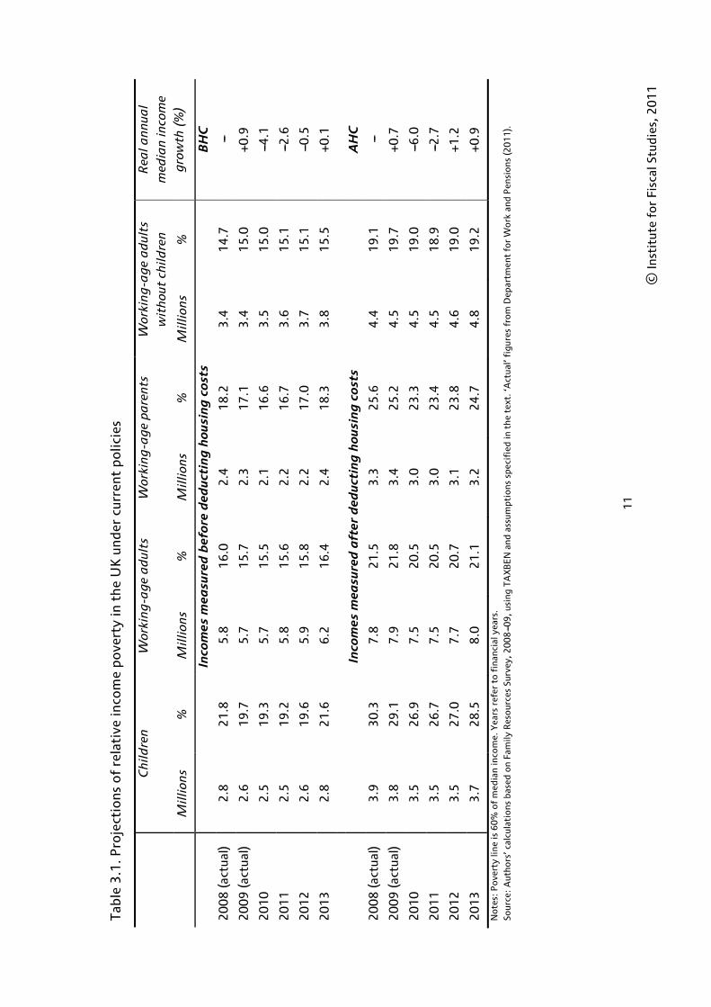
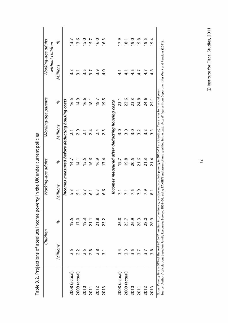
Tables 3.1 and 3.2 show our projections to 2013 of relative and absolute income poverty respectively using the 60% of median income poverty line (both before and after housing costs (BHC and AHC)), under current policies.9 We show projected poverty rates for four subgroups: children, working-age adults, working-age parents and working-age adults without dependent children. We split working-age adults into those with and those without dependent children because recent poverty trends have differed between these groups (and, indeed, the same is true under our projections). Table 3.1 also gives our projections of real annual growth in median household incomes.
The tables show the following:
• We estimate that real median household incomes have fallen significantly between 2009 and 2011. By reducing the relative poverty line, this reduces relative poverty, other things being equal.
• We expect that relative child poverty will have fallen by a further 100,000 in 2010 on top of the 200,000 fall seen in 2009 for incomes measured BHC and remain at this level in 2011. But relative poverty among working-age adults without dependent children is expected to rise slightly (by about 200,000 with incomes measured BHC) between 2009 and 2011, despite the fall in the relative poverty line.
• Absolute poverty is forecast to have remained relatively stable among families with dependent children, but to have increased among working-age adults without dependent children (by about 300,000 or 1 percentage point BHC), between 2008 and 2010. The fact that absolute poverty among families with dependent children is not forecast to have risen as the UK was emerging from recession is likely to be (at least partly) due to the previous government’s above-indexation Child Tax Credit increases over this period.10 In 2011, however, absolute child poverty is forecast to rise by 300,000.
9 Results using the 50% of median income poverty line and the 70% of median income poverty line are reported in Appendix D. The trends in these poverty rates are broadly equivalent to those reported here. 10 See Brewer, Browne, Joyce and Sutherland (2009) and Brewer, Browne, Joyce and Sibieta (2010).
11
© In
stit
ute
for
Fisc
al S
tudi
es, 2
01
1
Tabl
e 3.
1. P
roje
ctio
ns o
f re
lati
ve in
com
e po
vert
y in
the
UK
und
er c
urre
nt p
olic
ies
C
hild
ren
W
orki
ng
-ag
e a
dul
ts
Wor
kin
g-a
ge
pare
nts
W
orki
ng
-ag
e a
dul
ts
wit
hou
t ch
ildre
n
Rea
l an
nua
l m
edia
n in
com
e g
row
th (
%)
M
illio
ns
%
Mill
ion
s %
M
illio
ns
%
Mill
ion
s %
In
com
es m
easu
red
bef
ore
ded
ucti
ng
hou
sin
g c
osts
B
HC
20
08
(ac
tual
) 2
.8
21
.8
5.8
1
6.0
2
.4
18
.2
3.4
1
4.7
---
20
09
(ac
tual
) 2
.6
19
.7
5.7
1
5.7
2
.3
17
.1
3.4
1
5.0
+0
.9
20
10
2.5
1
9.3
5
.7
15
.5
2.1
1
6.6
3
.5
15
.0
---4.1
20
11
2.5
1
9.2
5
.8
15
.6
2.2
1
6.7
3
.6
15
.1
---2.6
20
12
2.6
1
9.6
5
.9
15
.8
2.2
1
7.0
3
.7
15
.1
---0.5
20
13
2.8
2
1.6
6
.2
16
.4
2.4
1
8.3
3
.8
15
.5
+0.1
Inco
mes
mea
sure
d a
fter
ded
ucti
ng
hou
sin
g c
osts
A
HC
20
08
(ac
tual
) 3
.9
30
.3
7.8
2
1.5
3
.3
25
.6
4.4
1
9.1
---
20
09
(ac
tual
) 3
.8
29
.1
7.9
2
1.8
3
.4
25
.2
4.5
1
9.7
+0
.7
20
10
3.5
2
6.9
7
.5
20
.5
3.0
2
3.3
4
.5
19
.0
---6.0
20
11
3.5
2
6.7
7
.5
20
.5
3.0
2
3.4
4
.5
18
.9
---2.7
20
12
3.5
2
7.0
7
.7
20
.7
3.1
2
3.8
4
.6
19
.0
+1.2
20
13
3.7
2
8.5
8
.0
21
.1
3.2
2
4.7
4
.8
19
.2
+0.9
No
tes:
Po
vert
y lin
e is
60%
of
med
ian
inco
me.
Yea
rs r
efer
to
fin
anci
al y
ears
. So
urce
: A
utho
rs’ c
alcu
lati
ons
bas
ed o
n Fa
mily
Res
our
ces
Surv
ey, 2
00
8---0
9, u
sing
TA
XB
EN
and
ass
umpt
ions
spe
cifi
ed in
the
tex
t. ‘A
ctua
l’ fi
gure
s fr
om
Dep
artm
ent
for
Wo
rk a
nd P
ensi
ons
(20
11).
12
© In
stit
ute
for
Fisc
al S
tudi
es, 2
01
1
Tabl
e 3
.2. P
roje
ctio
ns o
f ab
solu
te in
com
e po
vert
y in
the
UK
und
er c
urre
nt p
olic
ies
C
hild
ren
W
orki
ng
-ag
e a
dul
ts
Wor
kin
g-a
ge
pare
nts
W
orki
ng
-ag
e a
dul
ts
wit
hou
t ch
ildre
n
M
illio
ns
%
Mill
ion
s %
M
illio
ns
%
Mill
ion
s %
In
com
es m
easu
red
bef
ore
ded
ucti
ng
hou
sin
g c
osts
20
08
(ac
tual
) 2
.5
19
.5
5.3
1
4.7
2
.1
16
.5
3.2
1
3.7
20
09
(ac
tual
) 2
.2
17
.0
5.1
1
4.1
2
.0
14
.9
3.1
1
3.6
20
10
2.5
1
9.3
5
.7
15
.5
2.1
1
6.6
3
.5
15
.0
20
11
2.8
2
1.1
6
.1
16
.6
2.4
1
8.1
3
.7
15
.7
20
12
2.8
2
1.8
6
.3
16
.9
2.4
1
8.7
3
.9
16
.0
20
13
3.1
2
3.2
6
.6
17
.4
2.5
1
9.5
4
.0
16
.3
In
com
es m
easu
red
aft
er d
educ
tin
g h
ousi
ng
cos
ts
20
08
(ac
tual
) 3
.4
26
.8
7.1
1
9.7
3
.0
23
.1
4.1
1
7.9
20
09
(ac
tual
) 3
.3
25
.7
7.1
1
9.8
3
.0
22
.6
4.1
1
8.1
20
10
3.5
2
6.9
7
.5
20
.5
3.0
2
3.3
4
.5
19
.0
20
11
3.7
2
8.3
7
.9
21
.6
3.2
2
4.8
4
.7
19
.8
20
12
3.7
2
8.0
7
.9
21
.3
3.2
2
4.6
4
.7
19
.5
20
13
3.8
2
8.9
8
.1
21
.4
3.3
2
5.1
4
.8
19
.4
Not
es:
Pov
erty
line
is 6
0%
of
the
real
20
10
---11
med
ian
inco
me
(hen
ce, r
elat
ive
and
abso
lute
pov
erty
in 2
01
0---1
1 ar
e id
enti
cal)
. Yea
rs r
efer
to
fina
ncia
l yea
rs.
Sour
ce:
Aut
hors
’ cal
cula
tio
ns b
ased
on
Fam
ily R
eso
urce
s Su
rvey
, 20
08
---09
, usi
ng T
AX
BE
N a
nd a
ssum
ptio
ns s
peci
fied
in t
he t
ext.
‘Act
ual’
figu
res
fro
m D
epar
tmen
t fo
r W
ork
and
Pen
sio
ns (
2011
).
Results
13
© Institute for Fiscal Studies, 2011
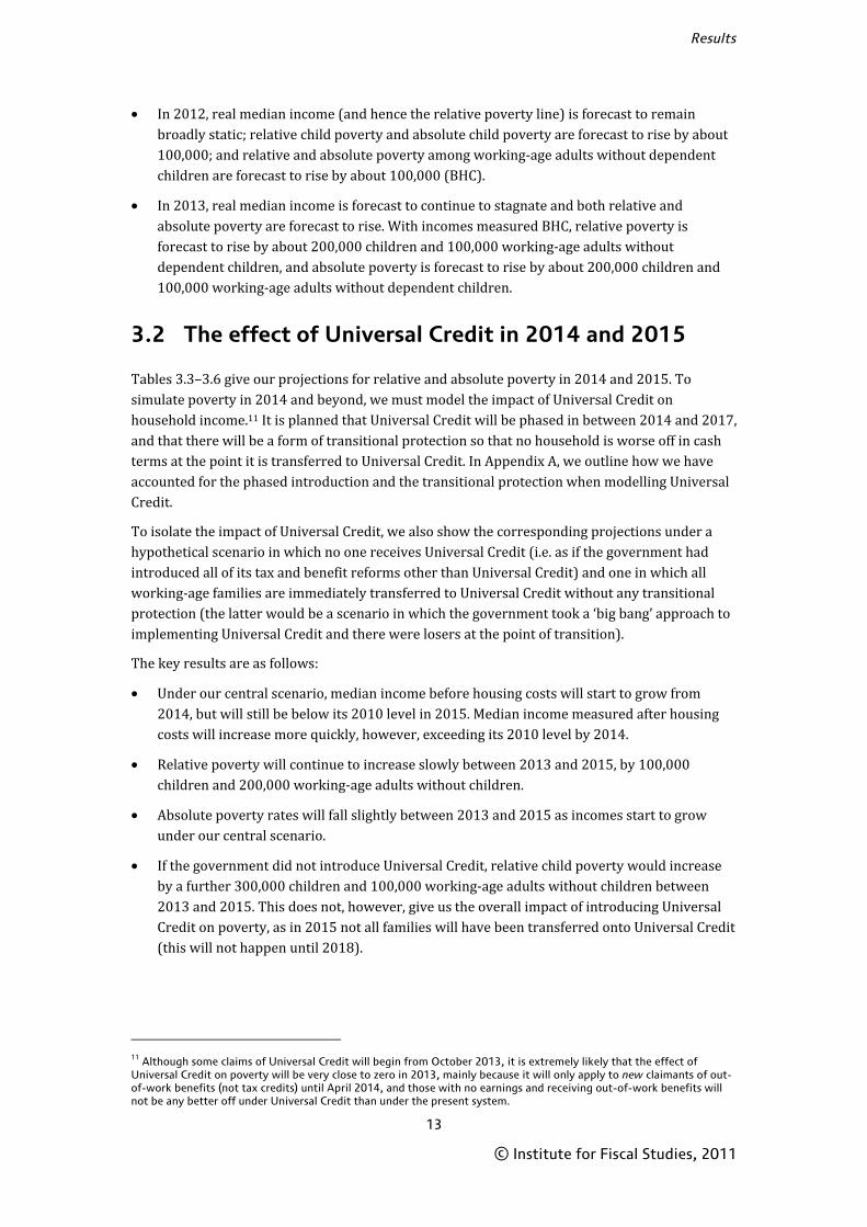
• In 2012, real median income (and hence the relative poverty line) is forecast to remain broadly static; relative child poverty and absolute child poverty are forecast to rise by about 100,000; and relative and absolute poverty among working-age adults without dependent children are forecast to rise by about 100,000 (BHC).
• In 2013, real median income is forecast to continue to stagnate and both relative and absolute poverty are forecast to rise. With incomes measured BHC, relative poverty is forecast to rise by about 200,000 children and 100,000 working-age adults without dependent children, and absolute poverty is forecast to rise by about 200,000 children and 100,000 working-age adults without dependent children.
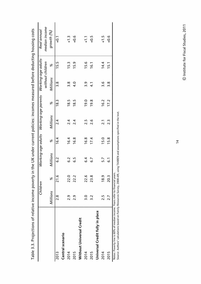
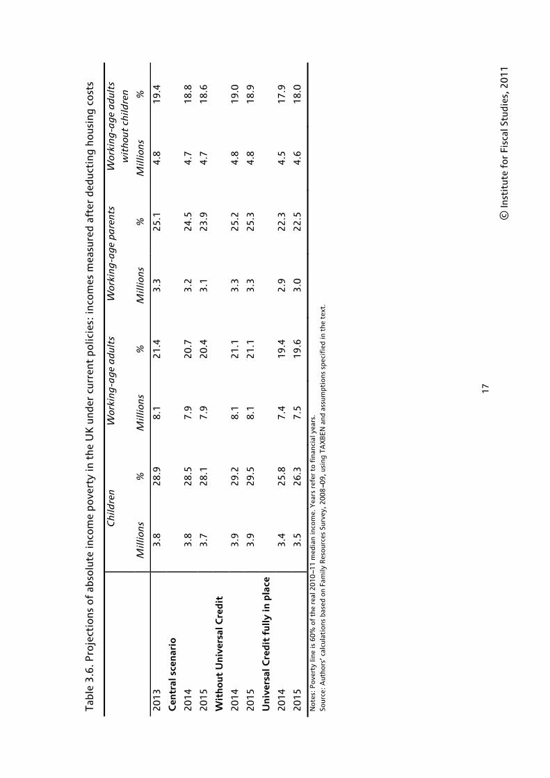
3.2 The effect of Universal Credit in 2014 and 2015
Tables 3.3–3.6 give our projections for relative and absolute poverty in 2014 and 2015. To simulate poverty in 2014 and beyond, we must model the impact of Universal Credit on household income.11 It is planned that Universal Credit will be phased in between 2014 and 2017, and that there will be a form of transitional protection so that no household is worse off in cash terms at the point it is transferred to Universal Credit. In Appendix A, we outline how we have accounted for the phased introduction and the transitional protection when modelling Universal Credit.
To isolate the impact of Universal Credit, we also show the corresponding projections under a hypothetical scenario in which no one receives Universal Credit (i.e. as if the government had introduced all of its tax and benefit reforms other than Universal Credit) and one in which all working-age families are immediately transferred to Universal Credit without any transitional protection (the latter would be a scenario in which the government took a ‘big bang’ approach to implementing Universal Credit and there were losers at the point of transition).
The key results are as follows:
• Under our central scenario, median income before housing costs will start to grow from 2014, but will still be below its 2010 level in 2015. Median income measured after housing costs will increase more quickly, however, exceeding its 2010 level by 2014.
• Relative poverty will continue to increase slowly between 2013 and 2015, by 100,000 children and 200,000 working-age adults without children.
• Absolute poverty rates will fall slightly between 2013 and 2015 as incomes start to grow under our central scenario.
• If the government did not introduce Universal Credit, relative child poverty would increase by a further 300,000 children and 100,000 working-age adults without children between 2013 and 2015. This does not, however, give us the overall impact of introducing Universal Credit on poverty, as in 2015 not all families will have been transferred onto Universal Credit (this will not happen until 2018).
11 Although some claims of Universal Credit will begin from October 2013, it is extremely likely that the effect of Universal Credit on poverty will be very close to zero in 2013, mainly because it will only apply to new claimants of out-of-work benefits (not tax credits) until April 2014, and those with no earnings and receiving out-of-work benefits will not be any better off under Universal Credit than under the present system.
14
© In
stit
ute
for
Fisc
al S
tudi
es, 2
01
1
Tabl
e 3.
3. P
roje
ctio
ns o
f re
lati
ve in
com
e po
vert
y in
the
UK
und
er c
urre
nt p
olic
ies:
inco
mes
mea
sure
d be
fore
ded
ucti
ng h
ousi
ng c
osts
C
hild
ren
W
orki
ng
-ag
e a
dul
ts
Wor
kin
g-a
ge
pare
nts
Wor
kin
g-a
ge
ad
ults
w
ith
out
child
ren
R
eal a
nn
ual
med
ian
inco
me
gro
wth
(%
)
Mill
ion
s %
M
illio
ns
%
Mill
ion
s %
M
illio
ns
%
20
13
2.8
2
1.6
6
.2
16
.4
2.4
1
8.3
3
.8
15
.5
+0.1
Cen
tral
sce
nar
io
20
14
2.9
2
2.0
6
.2
16
.4
2.4
1
8.5
3
.8
15
.3
+1.3
20
15
2.9
2
2.2
6
.5
16
.8
2.4
1
8.5
4
.0
15
.9
+0.6
Wit
ho
ut U
niv
ersa
l Cre
dit
20
14
3.0
2
2.6
6
.4
16
.8
2.5
1
9.0
3
.9
15
.6
+1.1
20
15
3.2
2
3.8
6
.7
17
.4
2.6
1
9.8
4
.1
16
.1
+0.5
Un
iver
sal C
red
it f
ully
in p
lace
20
14
2.5
1
8.9
5
.7
15
.0
2.1
1
6.2
3
.6
14
.4
+1.5
20
15
2.7
2
0.3
6
.1
15
.8
2.3
1
7.2
3
.8
15
.1
+0.6
No
tes:
Po
vert
y lin
e is
60%
of
med
ian
inco
me.
Yea
rs r
efer
to
fin
anci
al y
ears
. So
urce
: A
utho
rs’ c
alcu
lati
ons
bas
ed o
n Fa
mily
Res
our
ces
Surv
ey, 2
00
8---0
9, u
sing
TA
XB
EN
and
ass
umpt
ions
spe
cifi
ed in
the
tex
t.

15
© In
stit
ute
for
Fisc
al S
tudi
es, 2
01
1
Tabl
e 3.
4. P
roje
ctio
ns o
f re
lati
ve in
com
e po
vert
y in
the
UK
und
er c
urre
nt p
olic
ies:
inco
mes
mea
sure
d af
ter
dedu
ctin
g ho
usin
g co
sts
C
hild
ren
W
orki
ng
-ag
e a
dul
ts
Wor
kin
g-a
ge
pare
nts
Wor
kin
g-a
ge
ad
ults
w
ith
out
child
ren
R
eal a
nn
ual
med
ian
inco
me
gro
wth
(%
)
Mill
ion
s %
M
illio
ns
%
Mill
ion
s %
M
illio
ns
%
20
13
3.7
2
8.5
8
.0
21
.1
3.2
2
4.7
4
.8
19
.2
+0.9
Cen
tral
sce
nar
io
20
14
3.8
2
9.1
8
.0
21
.0
3.3
2
5.0
4
.8
19
.0
+2.1
20
15
3.9
2
9.7
8
.2
21
.2
3.3
2
5.3
4
.9
19
.2
+1.4
Wit
ho
ut U
niv
ersa
l Cre
dit
20
14
3.9
2
9.7
8
.2
21
.3
3.3
2
5.6
4
.8
19
.1
+1.9
20
15
4.1
3
1.0
8
.4
21
.8
3.5
2
6.5
4
.9
19
.4
+1.3
Un
iver
sal C
red
it f
ully
in p
lace
20
14
3.5
2
6.6
7
.6
19
.8
3.0
2
2.9
4
.6
18
.2
+2.2
20
15
3.7
2
8.0
7
.9
20
.5
3.1
2
3.9
4
.8
18
.8
+1.4
No
tes:
Po
vert
y lin
e is
60%
of
med
ian
inco
me.
Yea
rs r
efer
to
fin
anci
al y
ears
. So
urce
: A
utho
rs’ c
alcu
lati
ons
bas
ed o
n Fa
mily
Res
our
ces
Surv
ey, 2
00
8---0
9, u
sing
TA
XB
EN
and
ass
umpt
ions
spe
cifi
ed in
the
tex
t.

16
© In
stit
ute
for
Fisc
al S
tudi
es, 2
01
1
Tabl
e 3
.5. P
roje
ctio
ns o
f ab
solu
te in
com
e po
vert
y in
the
UK
und
er c
urre
nt p
olic
ies:
inco
mes
mea
sure
d be
fore
ded
ucti
ng h
ousi
ng c
osts
C
hild
ren
W
orki
ng
-ag
e a
dul
ts
Wor
kin
g-a
ge
pare
nts
W
orki
ng
-ag
e a
dul
ts
wit
hou
t ch
ildre
n
M
illio
ns
%
Mill
ion
s %
M
illio
ns
%
Mill
ion
s %
20
13
3.1
2
3.2
6
.6
17
.4
2.5
1
9.5
4
.0
16
.3
Cen
tral
sce
nar
io
20
14
3.0
2
2.9
6
.5
17
.1
2.5
1
9.2
4
.0
16
.0
20
15
3.0
2
2.8
6
.6
17
.1
2.5
1
9.0
4
.1
16
.0
Wit
ho
ut U
niv
ersa
l Cre
dit
20
14
3.1
2
3.8
6
.7
17
.5
2.6
1
9.9
4
.1
15
.9
20
15
3.3
2
4.6
6
.9
17
.8
2.7
2
0.4
4
.2
16
.5
Un
iver
sal C
red
it f
ully
in p
lace
20
14
2.6
1
9.9
5
.9
15
.5
2.2
1
7.0
3
.7
14
.7
20
15
2.8
2
1.0
6
.2
16
.1
2.3
1
7.8
3
.9
15
.3
Not
es:
Pov
erty
line
is 6
0%
of
the
real
20
10
---11
med
ian
inco
me.
Yea
rs r
efer
to
fina
ncia
l yea
rs.
Sour
ce:
Aut
hors
’ cal
cula
tio
ns b
ased
on
Fam
ily R
eso
urce
s Su
rvey
, 20
08
---09
, usi
ng T
AX
BE
N a
nd a
ssum
ptio
ns s
peci
fied
in t
he t
ext.
17
© In
stit
ute
for
Fisc
al S
tudi
es, 2
01
1
Tabl
e 3
.6. P
roje
ctio
ns o
f ab
solu
te in
com
e po
vert
y in
the
UK
und
er c
urre
nt p
olic
ies:
inco
mes
mea
sure
d af
ter
dedu
ctin
g ho
usin
g co
sts
C
hild
ren
W
orki
ng
-ag
e a
dul
ts
Wor
kin
g-a
ge
pare
nts
W
orki
ng
-ag
e a
dul
ts
wit
hou
t ch
ildre
n
M
illio
ns
%
Mill
ion
s %
M
illio
ns
%
Mill
ion
s %
20
13
3.8
2
8.9
8
.1
21
.4
3.3
2
5.1
4
.8
19
.4
Cen
tral
sce
nar
io
20
14
3.8
2
8.5
7
.9
20
.7
3.2
2
4.5
4
.7
18
.8
20
15
3.7
2
8.1
7
.9
20
.4
3.1
2
3.9
4
.7
18
.6
Wit
ho
ut U
niv
ersa
l Cre
dit
20
14
3.9
2
9.2
8
.1
21
.1
3.3
2
5.2
4
.8
19
.0
20
15
3.9
2
9.5
8
.1
21
.1
3.3
2
5.3
4
.8
18
.9
Un
iver
sal C
red
it f
ully
in p
lace
20
14
3.4
2
5.8
7
.4
19
.4
2.9
2
2.3
4
.5
17
.9
20
15
3.5
2
6.3
7
.5
19
.6
3.0
2
2.5
4
.6
18
.0
Not
es:
Pov
erty
line
is 6
0%
of
the
real
20
10
---11
med
ian
inco
me.
Yea
rs r
efer
to
fina
ncia
l yea
rs.
Sour
ce:
Aut
hors
’ cal
cula
tio
ns b
ased
on
Fam
ily R
eso
urce
s Su
rvey
, 20
08
---09
, usi
ng T
AX
BE
N a
nd a
ssum
ptio
ns s
peci
fied
in t
he t
ext.

Child and working-age poverty from 2010 to 2020
18
© Institute for Fiscal Studies, 2011
• By comparing the scenario in which Universal Credit is not introduced with the scenario in which Universal Credit is fully in place in 2014, we can see that the impact of introducing Universal Credit without any transitional protection or phase-in period in 2014 would be to lower relative child poverty by 450,000 and relative poverty among working-age adults by 600,000. DWP’s analysis of the effect of fully introducing Universal Credit in 2014 without any transitional protection or phase-in period produced a smaller estimate of the effect of the reform on child poverty, though our estimates are the same for working-age adults.12
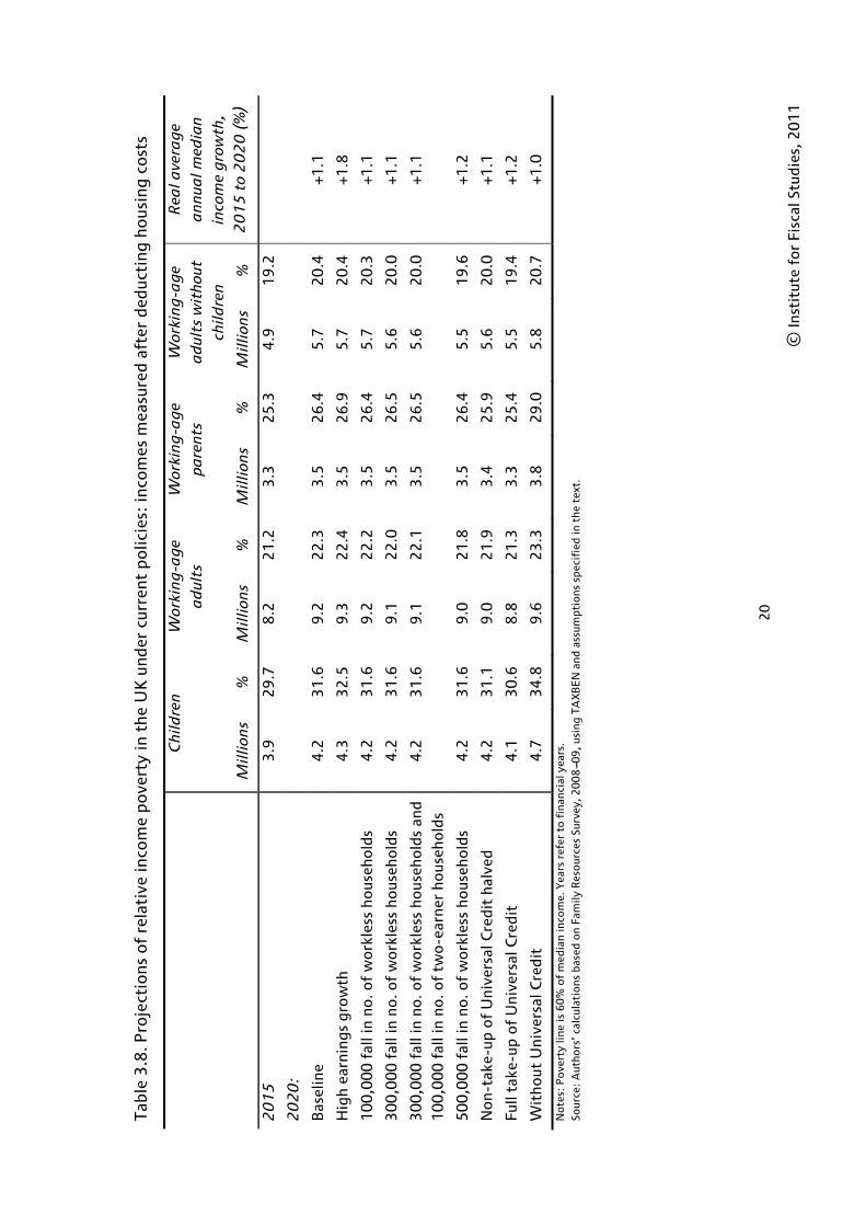
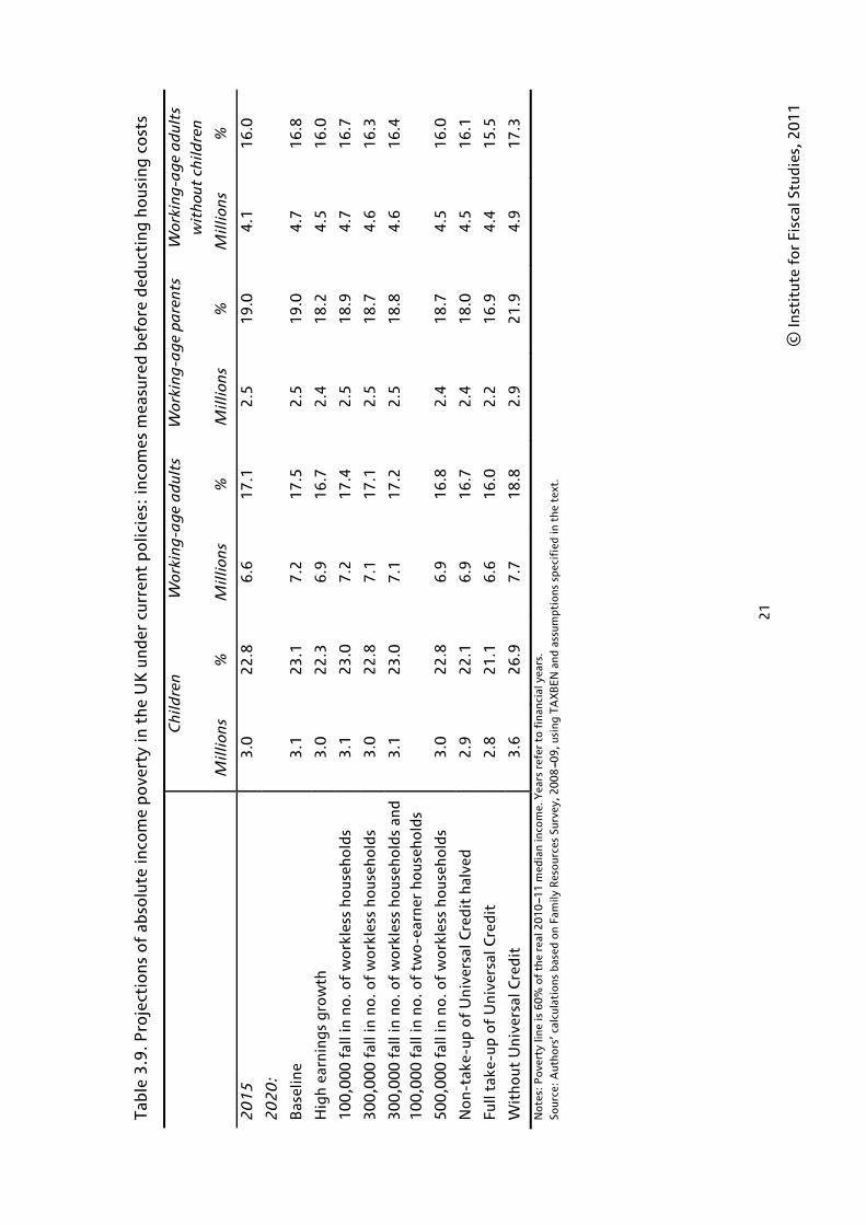
3.3 Projections of poverty in 2020 under different scenarios
Our main assumptions about the evolution of macroeconomic variables up to 2020 are set out in Appendix A. Clearly, there are many uncertainties when projecting so far into the future, so we examine the sensitivity of our projections to our assumptions about employment and earnings and we examine the effect of higher take-up of Universal Credit. Further sensitivity analysis for our 2015 projections can be found in Appendix B.
Tables 3.7 to 3.10 show poverty projections under each of these scenarios. The key results are as follows:
• In our baseline scenario, relative poverty is forecast to continue to increase between 2015 and 2020, by 300,000 children and 1 million working-age adults. This increase is mainly due to benefit rates not keeping pace with growth in median income – CPI-uprating of benefits means that they go up by 1.5 percentage points less than the RPI over this period and 2.5 percentage points less each year than gross earnings in our baseline scenario. This means that the difference in incomes between low-income households (who are more reliant on income from the state) and households around the median (who are more reliant on earnings) tends to increase over time, increasing relative poverty. However, the completion of the introduction of Universal Credit over this period limits the increase in poverty somewhat.
• Absolute poverty rates remain fairly constant between 2015 and 2020, despite earnings (and median income) rising in real terms. It is likely that this is again because the CPI-indexation of benefits lags behind the RPI-indexation of the absolute poverty line.
• Our projections are remarkably insensitive to changes in employment rates and take-up that might result from the introduction of Universal Credit. In theory, increased employment unambiguously reduces absolute poverty, but it might actually increase relative poverty, because it may raise median income and hence the relative poverty line.13 Furthermore, starting paid work is sometimes not sufficient for a household to escape poverty (indeed, as Jin, Joyce, Phillips and Sibieta (2011) show, 56% of children currently in poverty have at least one working parent). Our baseline scenario incorporates a high level of take-up of Universal Credit to begin with, meaning that there is little scope for higher take-up to reduce poverty further.
12 See Department for Work and Pensions (2011). The reasons for this small discrepancy are not clear. We have received a considerable amount of advice from DWP officials on how best to model Universal Credit in our tax and benefit microsimulation model, but we have not been able to verify that our approach was identical to the one they took when producing estimates earlier this year. 13 Of course, a rise in employment concentrated amongst groups who experience high rates of poverty when out of work can lower relative poverty.

19
© In
stit
ute
for
Fisc
al S
tudi
es, 2
01
1
Tabl
e 3.
7. P
roje
ctio
ns o
f re
lati
ve in
com
e po
vert
y in
20
20
und
er d
iffe
rent
sce
nari
os:
inco
mes
mea
sure
d be
fore
ded
ucti
ng h
ousi
ng c
osts
C
hild
ren
W
orki
ng
-ag
e a
dul
ts
Wor
kin
g-a
ge
pare
nts
W
orki
ng
-ag
e a
dul
ts w
itho
ut
child
ren
Rea
l ave
rag
e a
nn
ual m
edia
n
inco
me
gro
wth
, 2
01
5 t
o 2
02
0 (
%)
M
illio
ns
%
Mill
ion
s %
M
illio
ns
%
Mill
ion
s %
20
15
2
.9
22
.2
6.5
1
6.8
2
.4
18
.5
4.0
1
5.9
20
20
:
Bas
elin
e 3
.3
24
.4
7.5
1
8.3
2
.6
20
.0
4.9
1
7.5
+0
.5
Hig
h ea
rnin
gs g
row
th
3.5
2
5.9
7
.7
18
.6
2.7
2
0.9
4
.9
17
.5
+1.2
10
0,0
00 f
all i
n no
. of
wo
rkle
ss h
ous
eho
lds
3.3
2
4.4
7
.5
18
.2
2.6
2
0.0
4
.9
17
.4
+0.5
30
0,0
00 f
all i
n no
. of
wo
rkle
ss h
ous
eho
lds
3.3
2
4.4
7
.4
18
.0
2.6
2
0.0
4
.8
17
.1
+0.6
30
0,0
00 f
all i
n no
. of
wor
kles
s ho
useh
olds
and
1
00
,000
fal
l in
no. o
f tw
o-ea
rner
hou
seho
lds
3.3
2
4.6
7
.5
18
.1
2.6
2
0.1
4
.8
17
.2
+0.6
50
0,0
00 f
all i
n no
. of
wor
kles
s ho
useh
olds
3
.3
24
.5
7.3
1
7.8
2
.6
20
.0
4.7
1
6.8
+0
.6
No
n-ta
ke-u
p o
f U
nive
rsal
Cre
dit
halv
ed
3.1
2
3.6
7
.3
17
.7
2.5
1
9.2
4
.8
16
.9
+0.6
Full
take
-up
of
Uni
vers
al C
redi
t 3
.1
22
.8
7.0
1
6.9
2
.4
18
.3
4.6
1
6.3
+0
.6
Wit
hout
Uni
vers
al C
redi
t 3
.8
28
.1
8.0
1
9.4
3
.0
22
.9
5.0
1
7.8
+0
.5
No
tes:
Po
vert
y lin
e is
60%
of
med
ian
inco
me.
Yea
rs r
efer
to
fin
anci
al y
ears
. So
urce
: A
utho
rs’ c
alcu
lati
ons
bas
ed o
n Fa
mily
Res
our
ces
Surv
ey, 2
00
8---0
9, u
sing
TA
XB
EN
and
ass
umpt
ions
spe
cifi
ed in
the
tex
t.
20
© In
stit
ute
for
Fisc
al S
tudi
es, 2
01
1
Tabl
e 3.
8. P
roje
ctio
ns o
f re
lati
ve in
com
e po
vert
y in
the
UK
und
er c
urre
nt p
olic
ies:
inco
mes
mea
sure
d af
ter
dedu
ctin
g ho
usin
g co
sts
C
hild
ren
W
orki
ng
-ag
e a
dul
ts
Wor
kin
g-a
ge
pare
nts
W
orki
ng
-ag
e a
dul
ts w
itho
ut
child
ren
Rea
l ave
rag
e a
nn
ual m
edia
n
inco
me
gro
wth
, 2
01
5 t
o 2
02
0 (
%)
M
illio
ns
%
Mill
ion
s %
M
illio
ns
%
Mill
ion
s %
20
15
3
.9
29
.7
8.2
2
1.2
3
.3
25
.3
4.9
1
9.2
20
20
:
Bas
elin
e 4
.2
31
.6
9.2
2
2.3
3
.5
26
.4
5.7
2
0.4
+1
.1
Hig
h ea
rnin
gs g
row
th
4.3
3
2.5
9
.3
22
.4
3.5
2
6.9
5
.7
20
.4
+1.8
10
0,0
00 f
all i
n no
. of
wo
rkle
ss h
ous
eho
lds
4.2
3
1.6
9
.2
22
.2
3.5
2
6.4
5
.7
20
.3
+1.1
30
0,0
00 f
all i
n no
. of
wo
rkle
ss h
ous
eho
lds
4.2
3
1.6
9
.1
22
.0
3.5
2
6.5
5
.6
20
.0
+1.1
30
0,0
00 f
all i
n no
. of
wor
kles
s ho
useh
olds
and
1
00
,000
fal
l in
no. o
f tw
o-ea
rner
hou
seho
lds
4.2
3
1.6
9
.1
22
.1
3.5
2
6.5
5
.6
20
.0
+1.1
50
0,0
00 f
all i
n no
. of
wo
rkle
ss h
ous
eho
lds
4.2
3
1.6
9
.0
21
.8
3.5
2
6.4
5
.5
19
.6
+1.2
No
n-ta
ke-u
p o
f U
nive
rsal
Cre
dit
halv
ed
4.2
3
1.1
9
.0
21
.9
3.4
2
5.9
5
.6
20
.0
+1.1
Full
take
-up
of
Uni
vers
al C
redi
t 4
.1
30
.6
8.8
2
1.3
3
.3
25
.4
5.5
1
9.4
+1
.2
Wit
hout
Uni
vers
al C
redi
t 4
.7
34
.8
9.6
2
3.3
3
.8
29
.0
5.8
2
0.7
+1
.0
No
tes:
Po
vert
y lin
e is
60%
of
med
ian
inco
me.
Yea
rs r
efer
to
fin
anci
al y
ears
. So
urce
: A
utho
rs’ c
alcu
lati
ons
bas
ed o
n Fa
mily
Res
our
ces
Surv
ey, 2
00
8---0
9, u
sing
TA
XB
EN
and
ass
umpt
ions
spe
cifi
ed in
the
tex
t.
21
© In
stit
ute
for
Fisc
al S
tudi
es, 2
01
1
Tabl
e 3
.9. P
roje
ctio
ns o
f ab
solu
te in
com
e po
vert
y in
the
UK
und
er c
urre
nt p
olic
ies:
inco
mes
mea
sure
d be
fore
ded
ucti
ng h
ousi
ng c
osts
C
hild
ren
W
orki
ng
-ag
e a
dul
ts
Wor
kin
g-a
ge
pare
nts
W
orki
ng
-ag
e a
dul
ts
wit
hou
t ch
ildre
n
M
illio
ns
%
Mill
ion
s %
M
illio
ns
%
Mill
ion
s %
20
15
3
.0
22
.8
6.6
1
7.1
2
.5
19
.0
4.1
1
6.0
20
20
:
Bas
elin
e 3
.1
23
.1
7.2
1
7.5
2
.5
19
.0
4.7
1
6.8
Hig
h ea
rnin
gs g
row
th
3.0
2
2.3
6
.9
16
.7
2.4
1
8.2
4
.5
16
.0
10
0,0
00 f
all i
n no
. of
wo
rkle
ss h
ous
eho
lds
3.1
2
3.0
7
.2
17
.4
2.5
1
8.9
4
.7
16
.7
30
0,0
00 f
all i
n no
. of
wo
rkle
ss h
ous
eho
lds
3.0
2
2.8
7
.1
17
.1
2.5
1
8.7
4
.6
16
.3
30
0,0
00 f
all i
n no
. of
wor
kles
s ho
useh
olds
and
1
00
,000
fal
l in
no. o
f tw
o-ea
rner
hou
seho
lds
3.1
2
3.0
7
.1
17
.2
2.5
1
8.8
4
.6
16
.4
50
0,0
00 f
all i
n no
. of
wo
rkle
ss h
ous
eho
lds
3.0
2
2.8
6
.9
16
.8
2.4
1
8.7
4
.5
16
.0
No
n-ta
ke-u
p o
f U
nive
rsal
Cre
dit
halv
ed
2.9
2
2.1
6
.9
16
.7
2.4
1
8.0
4
.5
16
.1
Full
take
-up
of
Uni
vers
al C
redi
t 2
.8
21
.1
6.6
1
6.0
2
.2
16
.9
4.4
1
5.5
Wit
hout
Uni
vers
al C
redi
t 3
.6
26
.9
7.7
1
8.8
2
.9
21
.9
4.9
1
7.3
Not
es:
Pov
erty
line
is 6
0%
of
the
real
20
10
---11
med
ian
inco
me.
Yea
rs r
efer
to
fina
ncia
l yea
rs.
Sour
ce:
Aut
hors
’ cal
cula
tio
ns b
ased
on
Fam
ily R
eso
urce
s Su
rvey
, 20
08
---09
, usi
ng T
AX
BE
N a
nd a
ssum
ptio
ns s
peci
fied
in t
he t
ext.

22
© In
stit
ute
for
Fisc
al S
tudi
es, 2
01
1
Tabl
e 3
.10
. Pro
ject
ions
of
abso
lute
inco
me
pove
rty
in t
he U
K u
nder
cur
rent
pol
icie
s: in
com
es m
easu
red
afte
r de
duct
ing
hous
ing
cost
s
C
hild
ren
W
orki
ng
-ag
e a
dul
ts
Wor
kin
g-a
ge
pare
nts
W
orki
ng
-ag
e a
dul
ts
wit
hou
t ch
ildre
n
M
illio
ns
%
Mill
ion
s %
M
illio
ns
%
Mill
ion
s %
20
15
3
.7
28
.1
7.9
2
0.4
3
.1
23
.9
4.7
1
8.6
20
20
:
Bas
elin
e 3
.7
27
.4
8.2
1
9.8
3
.0
23
.1
5.1
1
8.2
Hig
h ea
rnin
gs g
row
th
3.5
2
6.6
7
.8
19
.0
2.9
2
2.3
4
.9
17
.5
10
0,0
00 f
all i
n no
. of
wo
rkle
ss h
ous
eho
lds
3.6
2
7.3
8
.1
19
.7
3.0
2
3.1
5
.1
18
.2
30
0,0
00 f
all i
n no
. of
wo
rkle
ss h
ous
eho
lds
3.6
2
7.1
8
.0
19
.4
3.0
2
2.9
5
.0
17
.8
30
0,0
00 f
all i
n no
. of
wor
kles
s ho
useh
olds
and
1
00
,000
fal
l in
no. o
f tw
o-ea
rner
hou
seho
lds
3.6
2
7.2
8
.0
19
.5
3.0
2
3.0
5
.0
17
.9
50
0,0
00 f
all i
n no
. of
wo
rkle
ss h
ous
eho
lds
3.6
2
7.0
7
.9
19
.2
3.0
2
2.7
4
.9
17
.5
No
n-ta
ke-u
p o
f U
nive
rsal
Cre
dit
halv
ed
3.5
2
6.6
7
.9
19
.2
2.9
2
2.3
5
.0
17
.7
Full
take
-up
of
Uni
vers
al C
redi
t 3
.4
25
.8
7.6
1
8.4
2
.8
21
.6
4.8
1
6.9
Wit
hout
Uni
vers
al C
redi
t 4
.2
31
.2
8.7
2
1.2
3
.4
26
.1
5.3
1
8.9
Not
es:
Pov
erty
line
is 6
0%
of
the
real
20
10
---11
med
ian
inco
me.
Yea
rs r
efer
to
fina
ncia
l yea
rs.
Sour
ce:
Aut
hors
’ cal
cula
tio
ns b
ased
on
Fam
ily R
eso
urce
s Su
rvey
, 20
08
---09
, usi
ng T
AX
BE
N a
nd a
ssum
ptio
ns s
peci
fied
in t
he t
ext.

Results
23
© Institute for Fiscal Studies, 2011
• If the government did not introduce Universal Credit, poverty would increase by much more over the period from 2015 to 2020. Relative poverty would be higher by 450,000 children and 600,000 working-age adults if Universal Credit were not introduced. Thus we see that the long-run impact of Universal Credit is to reduce relative poverty by around 450,000 children and 600,000 working-age adults (which happens to be equal to the estimated impact of introducing Universal Credit in 2014 without any phase-in or transitional protection that we saw in the previous section).
The Child Poverty Act 2010 commits current and future governments to reducing relative BHC income child poverty to 10%, and absolute BHC income child poverty to 5%, by 2020. Our results suggest that current policies will fall far short of this objective: we estimate that in 2020 relative child poverty will be at its highest rate since 1999 and absolute child poverty will be at its highest rate since 2001.
Figure 3.1. Absolute and relative child poverty
Notes: Years up to 1992 are calendar years; thereafter, years refer to financial years. Incomes are measured before housing costs have been deducted (BHC) and are equivalised using the modified OECD equivalence scale. Figures before 2001 are for Great Britain; figures from 2002 onwards are for the whole United Kingdom (Northern Ireland was first included in the official HBAI series in 2002---03). Years between 2015 and 2020 are linear interpolations between figures for 2015 and 2020. Sources: Figures for 1980 to 2009 are from the Family Expenditure Survey (1980---93) and the Family Resources Survey (1994---2009). Projections are authors’ calculations based on Family Resources Survey, 2008---09, using TAXBEN and assumptions specified in the text.
3.4 The direct impact on poverty of the coalition government’s tax and benefit reforms
In this section, we repeat the simulations presented so far in this chapter, except that the assumed tax and benefit systems are those that would have been in place if the coalition government had simply implemented the plans for the tax and benefit system that it inherited from the previous government. By comparing the results of these simulations with those in the previous sections, we can quantify the direct impact of those reforms on poverty between 2010 and 2015 and then in 2020.
It is very important to recognise what this exercise does and does not reveal. The tax and benefit systems that would have been in place if the coalition government had not made any reforms are
0%
5%
10%
15%
20%
25%
30%
1980 1985 1990 1995 2000 2005 2010 2015 2020
Chi
ld p
over
ty r
ate
Relative: actual
Relative: forecast
Relative: 2020 target
Absolute: actual
Absolute: forecast
Absolute: 2020 target

Child and working-age poverty from 2010 to 2020
24
© Institute for Fiscal Studies, 2011
not necessarily the same as the systems that would have been in place if the previous government had remained in office. Given the UK’s fiscal position, it is highly likely that any incoming government would have made tax and benefit reforms beyond those that had been announced before the 2010 general election. Thus, just as the title of this section suggests, we are quantifying the direct impact of the coalition government’s reforms; we are not comparing the coalition’s reforms with the reforms of a hypothetical Labour administration (and, indeed, there is no way we could credibly do so, since we do not know what those reforms would have been).
Note also that these simulations take as given the expected macroeconomic environment, according to the economic forecasts published by the Office for Budget Responsibility (OBR) alongside Budget 2011. If the coalition government’s tax and benefit reforms have (positive or negative) impacts on macroeconomic variables such as employment and earnings between 2010 and 2015, then in reality that will have an impact on poverty (though the nature of that impact, particularly on relative poverty, would depend on the distribution of employment and earnings effects). The nature of these macroeconomic effects is unclear, so we ignore these possibilities here. However, we do explore the sensitivity of our poverty forecasts to assumptions about earnings and employment in Chapter 4. A related point is that the higher inflation caused by the VAT rise in January 2011 could lead to higher benefit rates in 2012 than would otherwise have been the case, because the uprating of most benefits in April 2012 will be based on CPI inflation in September 2011. On the other hand, the Bank of England has a 2% CPI inflation target: predicting the effect of the VAT rise on benefit rates would involve predicting the monetary policy response. We would also expect increases in the prices of goods to be accompanied by increases in nominal earnings and thus median income, so the net effect on relative poverty is ambiguous. An increase in the general price level would also raise the absolute poverty line (because it is fixed in real terms); overall, the net effect of a VAT rise on absolute poverty is ambiguous.
Figures 3.2 to 3.5 show the results, comparing them with the projections obtained under current policies. We focus here on poverty among children and among working-age adults without dependent children. The numbers underlying these figures, as well as the corresponding numbers for working-age parents and all working-age adults, can be found in Appendix C.
The figures show the following:
• The coalition government’s reforms have a negligible net impact on relative and absolute poverty in 2011.
• The coalition government’s reforms act to increase poverty slightly in 2012. Those reforms increase relative child poverty by about 100,000, absolute child poverty by about 200,000, and absolute poverty among working-age adults without dependent children by about 100,000 (on a BHC basis).
• In 2013, our projections suggest that coalition reforms increase both relative and absolute poverty by about 300,000 children and 100,000 working-age adults without dependent children (on a BHC basis). The reforms explain virtually all of the predicted rise in absolute poverty between 2012 and 2013.
• Beyond 2013, reforms introduced by the coalition have a slightly smaller overall effect on relative child poverty, though we estimate there will be 200,000 more children in relative poverty in 2014, 2015 and 2020 than there would have been without the government’s reforms. This is because the introduction of Universal Credit, which significantly reduces relative poverty, is offset by the continued CPI-uprating of benefits. The effect of the coalition
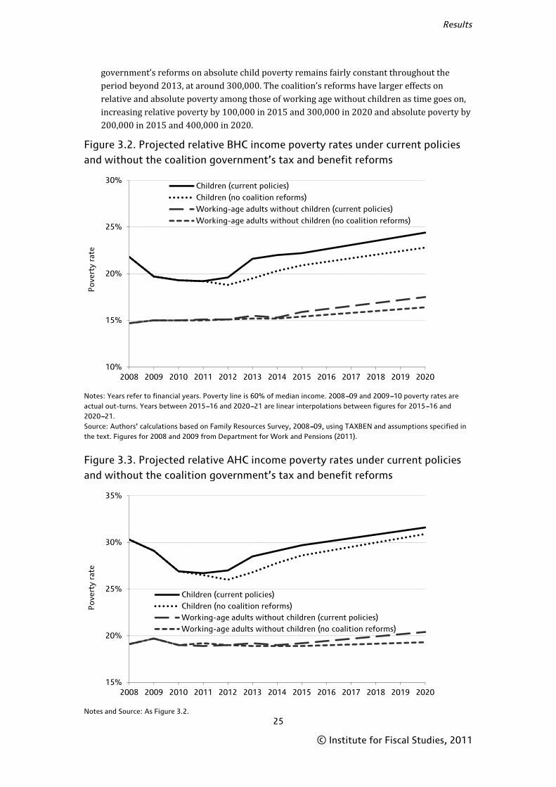
Results
25
© Institute for Fiscal Studies, 2011
government’s reforms on absolute child poverty remains fairly constant throughout the period beyond 2013, at around 300,000. The coalition’s reforms have larger effects on relative and absolute poverty among those of working age without children as time goes on, increasing relative poverty by 100,000 in 2015 and 300,000 in 2020 and absolute poverty by 200,000 in 2015 and 400,000 in 2020.
Figure 3.2. Projected relative BHC income poverty rates under current policies and without the coalition government’s tax and benefit reforms
Notes: Years refer to financial years. Poverty line is 60% of median income. 2008---09 and 2009---10 poverty rates are actual out-turns. Years between 2015---16 and 2020---21 are linear interpolations between figures for 2015---16 and 2020---21. Source: Authors’ calculations based on Family Resources Survey, 2008---09, using TAXBEN and assumptions specified in the text. Figures for 2008 and 2009 from Department for Work and Pensions (2011).
Figure 3.3. Projected relative AHC income poverty rates under current policies and without the coalition government’s tax and benefit reforms
Notes and Source: As Figure 3.2.
10%
15%
20%
25%
30%
2008 2009 2010 2011 2012 2013 2014 2015 2016 2017 2018 2019 2020
Po
vert
y ra
te
Children (current policies)Children (no coalition reforms)Working-age adults without children (current policies)Working-age adults without children (no coalition reforms)
15%
20%
25%
30%
35%
2008 2009 2010 2011 2012 2013 2014 2015 2016 2017 2018 2019 2020
Po
vert
y ra
te
Children (current policies)Children (no coalition reforms)Working-age adults without children (current policies)Working-age adults without children (no coalition reforms)

Child and working-age poverty from 2010 to 2020
26
© Institute for Fiscal Studies, 2011
Figure 3.4. Projected absolute BHC income poverty rates under current policies and without the coalition government’s tax and benefit reforms
Notes: Years refer to financial years. Poverty line is 60% of the real 2010---11 median income. 2008---09 and 2009---10 poverty rates are actual out-turns. Years between 2015---16 and 2020---21 are linear interpolations between figures for 2015---16 and 2020---21. Source: Authors’ calculations based on Family Resources Survey, 2008---09, using TAXBEN and assumptions specified in the text. Figures for 2008 and 2009 from Department for Work and Pensions (2011).
Figure 3.5. Projected absolute AHC income poverty rates under current policies and without the coalition government’s tax and benefit reforms
Notes: As Figure 3.4. Source: As Figure 3.4.
10%
15%
20%
25%
30%
2008 2009 2010 2011 2012 2013 2014 2015 2016 2017 2018 2019 2020
Po
vert
y ra
te
Children (current policies)Children (no coalition reforms)Working-age adults without children (current policies)Working-age adults without children (no coalition reforms)
15%
20%
25%
30%
35%
2008 2009 2010 2011 2012 2013 2014 2015 2016 2017 2018 2019 2020
Po
vert
y ra
te
Children (current policies)Children (no coalition reforms)Working-age adults without children (current policies)Working-age adults without children (no coalition reforms)

Results
27
© Institute for Fiscal Studies, 2011
The coalition government has claimed that ‘the Government’s modelled tax and welfare reforms could reduce child poverty by up to 50,000 in 2011–12 and 2012–13’.14 Our analysis suggests that, although the coalition government’s reforms have no discernible impact on child poverty in 2011, they act to increase child poverty slightly in 2012, by about 100,000 and 200,000 children for relative and absolute poverty respectively. This estimated impact on relative child poverty in 2012 is small and it is entirely accounted for by the Local Housing Allowance reforms which we model and the Treasury does not.15 The coalition government’s reforms to Local Housing Allowance are a significant component of the effect of the current government’s reforms on poverty in 2015 – without these changes, relative and absolute child poverty would be at the same level as they would have been without any of the government’s changes, and these reforms account for at least half of the effect of the current government’s policies on relative and absolute poverty among those of working age without children.
14 HM Treasury, 2011, p. 84. 15 Note, however, that our analysis is not strictly comparable to that of the Treasury. Though the methods used and assumptions made are extremely similar, they are not identical; for example, the Treasury does not account for non-take-up of benefits and tax credits.

28
© Institute for Fiscal Studies, 2011
4. Sensitivities
In this chapter, we investigate the sensitivity of our poverty projections in 2015 to alternative scenarios for total employment and average earnings growth to those outlined in the Office for Budget Responsibility’s forecasts, in an attempt to reflect the macroeconomic uncertainty that clearly exists. We also consider the impact of changing our assumption about the distribution of earnings growth: projections in Chapter 3 were obtained under the assumption that all earnings grow at the forecasted rate of average earnings growth. (Section 3.3 considered how poverty in 2020 would differ under some alternative scenarios.)
Total employment and average earnings
We consider ‘optimistic’ and ‘pessimistic’ macroeconomic scenarios, where both total employment and average earnings are higher and lower (respectively) than the OBR’s forecasts. In the ‘optimistic’ scenario, we assume that employment is 200,000 higher and that average earnings are 2% higher in 2015 than the OBR expects. In the ‘pessimistic’ scenario, we assume that employment is 200,000 lower and that average earnings are 2% lower in 2015 than the OBR expects.16
Differential earnings growth
We also consider what would happen if the rate of average earnings growth were as the OBR expects, but earnings growth across the distribution were not uniform. In other words, we assume that earnings in 2015 are lower in some earnings decile groups, and higher in others, than they would be if they grew at the rate of average earnings; and we do this such that average earnings remain the same as under our central assumptions. We consider both progressive and regressive patterns of earnings growth. For each decile group of the earnings distribution, the assumed percentage deviations from the level of earnings implied by our central assumptions are given in Table 4.1.17
Table 4.1. Differential earnings growth scenarios
Scenario Assumed % deviation in earnings relative to our central assumptions, by decile group of the earnings distribution
1 2 3 4 5 6 7 8 9 10
Progressive +6.5 +5.5 +4.5 +3.5 +2.5 +1.5 +0.5 ---0.5 ---1.5 ---2.5
Regressive ---6.5 ---5.5 ---4.5 ---3.5 ---2.5 ---1.5 ---0.5 +0.5 +1.5 +2.5
16 The OBR’s forecast for total employment in 2015 is 30 million. 17 Note that in previous work (Brewer, Browne, Joyce and Sutherland, 2009), when testing the sensitivity of our results to differential earnings growth, we used the actual pattern of differential earnings growth observed between 2001 and 2006. However, given recent macroeconomic events, there is reason to suspect that past patterns will be a poor guide to the near future. Therefore, here we simply choose markedly progressive and regressive scenarios to document the sensitivity.

Sensitivities
29
© Institute for Fiscal Studies, 2011
Table 4.2. Projections of relative BHC income poverty in 2015: sensitivity analysis
Scenario Children Working-age adults without children
Median income (2010 prices)
Millions % Millions %
Baseline 2.9 22.2 4.0 15.9 £411 p.w.
High employment and earnings 3.0 22.8 4.0 15.8 £416 p.w.
Low employment and earnings 2.9 21.5 4.0 15.8 £404 p.w.
Progressive earnings growth 3.0 22.4 4.0 15.6 £414 p.w.
Regressive earnings growth 2.9 22.0 4.1 15.9 £408 p.w.
Note: The ‘scenarios’ are defined in the text. Source: Authors’ calculations based on Family Resources Survey, 2008---09, using TAXBEN and assumptions specified in the text.
Table 4.3. Projections of absolute BHC income poverty in 2015: sensitivity analysis
Scenario Children Working-age adults without children
Millions % Millions %
Baseline 3.0 22.8 4.1 16.0
High employment and earnings 3.0 22.5 4.0 15.7
Low employment and earnings 3.1 23.3 4.2 16.7
Progressive earnings growth 3.0 22.4 4.0 15.6
Regressive earnings growth 3.1 23.1 4.2 16.4
Note: As Table 4.2. Source: As Table 4.2.
Tables 4.2 and 4.3 show the results of these sensitivity tests for the cases of relative and absolute BHC income poverty in 2015, comparing them with the results obtained under our central assumptions (see Section 3.2). The tables show the following:
• Higher employment and average earnings act to increase relative poverty slightly among families with dependent children and have no discernible impact on relative poverty among working-age adults without dependent children. The former finding is consistent with that in Brewer, Browne, Joyce and Sutherland (2009) and is explained by the fact that higher employment and average earnings tend to raise the median income (and hence the relative poverty line) by more than they raise the incomes of low-income families with dependent children. Note that, by controlling for employment by reweighting the data, we have effectively assumed that the demographic composition of the employed population remains constant when total employment changes. Clearly, if employment changes by more among particular groups, this could have different implications for poverty.
• For both children and working-age adults without children, there is roughly a 1 percentage point reduction in absolute poverty for a 4% increase in average earnings or an increase in employment of 400,000 (comparing the second and third rows of Table 4.3).

Child and working-age poverty from 2010 to 2020
30
© Institute for Fiscal Studies, 2011
The progressive and regressive earnings growth scenarios have counterintuitive implications for relative child poverty, with the regressive scenario resulting in a lower relative child poverty rate than the progressive scenario. This highlights very acutely the importance for relative poverty of factors affecting the median income. Under the progressive earnings growth scenario, median income increases, which acts to increase relative child poverty (other things being equal); and this more than offsets the impact of higher earnings for low-income working parents. The intuition behind this result is that the median-income household is in the bottom half of the earnings distribution, because there are fewer workers in the bottom half of the income distribution than in the top half. Therefore, the median household gains a lot under a progressive pattern of earnings growth, whereas households lower down the income distribution (who are less likely to be working) gain less. Also, those with low individual earnings are not necessarily in low-income households: many minimum-wage and low earners have higher-earning partners or live in households with others in paid work. Indeed, as Figure 4.1 (from Brewer, May and Phillips (2009)) shows, the heaviest concentration of those earning the minimum wage in the income distribution is in the third income decile group, just above the poverty line (meaning these families are not in poverty in the first place), and many are in the top half of the income distribution (meaning that increases in their earnings would increase median income).
The progressive and regressive earnings growth scenarios have the expected effects on absolute poverty, with a progressive pattern acting to lower absolute poverty and a regressive pattern acting to increase it. The effects are small, however. This is because many people around the poverty line are not in work, so they are unaffected by patterns of earnings growth.
Figure 4.1. The position of families where someone earns the National Minimum Wage in the working-age income distribution
Source: Brewer, May and Phillips, 2009.
0.00
0.05
0.10
0.15
0.20
0.25
0.30
0.35
0.40
0.45
1 2 3 4 5 6 7 8 9 10
Pro
port
ion
of f
amili
es
Income decile
Inactive Min Wage Above

31
© Institute for Fiscal Studies, 2011
5. Conclusion
In this Commentary, we have produced projections of relative and absolute income poverty among children and working-age adults for each year between 2010–11 and 2015–16 and for 2020–21.
The trends in the short run are unusual in that measures of absolute poverty are set to increase by more than measures of relative poverty. This unusual pattern arises because the living standards of low-income families are set to fall over this period – which will increase absolute poverty – but they are forecast to fall by less than the living standards of families at median income, and so relative poverty is forecast to have fallen in 2010–11. Indeed, at its low point, real median household income is forecast to be 7% lower in 2012–13 than it was in 2009–10, and to remain below its 2009–10 level until at least 2015–16.
Between 2013–14 and 2015–16, absolute poverty is forecast to fall slightly, and relative poverty to rise slightly as real earnings return to positive growth. Between 2015–16 and 2020–21, all measures of poverty rise or remain broadly unchanged. These forecasts imply that relative child poverty will rise from its current level of 20% to reach 24% in 2020–21, and that child poverty against the fixed 2010–11 poverty line will reach 23% in 2020–21. These are both considerably higher than the targets specified in the 2010 Child Poverty Act (of 10% and 5% respectively), and the rate of relative child poverty forecast for 2020–21 would be the highest since 1999–2000.
These central forecasts account for the government policy towards personal tax and state benefits announced as of Summer 2011. We have also estimated the impact on poverty of the coalition government’s reforms by comparing these central forecasts with a forecast that assumes that none of the reforms announced by the current government is introduced. This comparison suggests that the impact of changes to personal tax and benefit policy announced by this coalition government – including Universal Credit and other changes announced but not yet implemented – is to increase relative child poverty by 200,000 in both 2015–16 and 2020–21, and to increase relative poverty for working-age adults by 200,000 in 2015–16 and 400,000 in 2020–21. The reforms are forecast to increase absolute child poverty by 300,000 in both 2015–16 and 2020–21, and to increase absolute working-age poverty by 300,000 in 2015–16 and 700,000 in 2020–21.
The most significant reform to state benefits proposed by the government is to replace all means-tested benefits and tax credits for those of working age with a single, integrated benefit to be known as Universal Credit. Considered in isolation, Universal Credit should reduce relative poverty significantly (by 450,000 children and 600,000 working-age adults), but this reduction is more than offset by the poverty-increasing impact of the government’s other changes to personal taxes and state benefits. The most important of these other changes for poverty in 2020–21 is that benefits, including the Local Housing Allowance from April 2013, will now be indexed in line with the CPI measure of inflation, rather than one derived from the RPI.
The government currently prefers to use the retail price index (RPI) to adjust the absolute poverty line for changes in prices over time, but it now uses the consumer price index (CPI) to adjust the generosity of most benefits and tax credits. It is well known that the CPI usually gives a lower estimate of the rate of inflation than the RPI, and this is one reason why absolute poverty is forecast to rise even between 2015–16 and 2020–21. Researchers continue to debate whether the RPI or the CPI gives a better measure of poorer households’ inflation experiences, but as the government apparently believes that the CPI is superior, given its policy on uprating benefits, it should consider indexing the absolute poverty line in line with the CPI as well.
Child and working-age poverty from 2010 to 2020
32
© Institute for Fiscal Studies, 2011
This Commentary forecasts what might happen to poverty under current government policies and shows that governments cannot rely on higher earnings and employment to reduce relative measures of poverty. The results therefore suggest that there can be almost no chance of eradicating child poverty – as defined in the Child Poverty Act 2010 – on current government policy. And, although this project did not assess what policies would be required in order for child poverty to be eradicated, it is impossible to see how relative child poverty could fall by so much in the next 10 years without changes to the labour market and welfare policy, and an increase in the amount of redistribution performed by the tax and benefit system, both to an extent never-before seen in the UK. IFS researchers have always argued that the targets set in the Child Poverty Act were extremely challenging, and the findings here confirm that view. It now seems almost incredible that the targets can be met, yet the government confirmed its commitment to them earlier this year, in its first Child Poverty Strategy, and remains legally-bound to hit them. We suggest the government consider whether it would be more productive to set itself realistic targets for child poverty and provide concrete suggestions for how they might be hit – ideally, verified with a quantitative modelling exercise such as this one.

33
© Institute for Fiscal Studies, 2011
Appendix A. Details of assumptions and modelling procedures
In this appendix, we first outline the key stages involved in producing our poverty projections (Section A.1). We then elaborate on some particular details of the modelling (Section A.2) and set out how we account for some of the preannounced policy changes whose effect on the distribution of incomes cannot be modelled straightforwardly using TAXBEN (Section A.3). Finally, we outline the general limitations of this work (Section A.4).
A.1 The basic approach
We simulate the whole distribution of household incomes in the UK in future years, using a definition of income as close as possible to that used for official measures of poverty. In doing this, we estimate the two things that define the number of individuals in relative poverty: the median household income, which determines the relative poverty line, and the number of individuals with a household income below that relative poverty line. Poverty projections are obtained directly from our simulated income distribution: we simply count the number of children or working-age adults whose household income is less than 60% of the national median. In the case of absolute poverty, we count the number of children or working-age adults whose simulated household income is below the absolute poverty line, which is fixed in real terms.
The methods by which we simulate the household income distribution are best understood as a number of steps, outlined below.
Data
We use data on 25,003 households in the UK from the 2008–09 Family Resources Survey (the most recent available for analysts to use at the time of writing). Crucially for our purposes, this contains information about private income sources and other characteristics that determine tax liabilities and benefit and tax credit entitlements. It is the same data set that is used to provide official poverty statistics in the UK. This is important, given that we are forecasting poverty as it is officially measured.
We use the 2008–09 FRS as our ‘base data’ on the UK distribution of household incomes, from which we project forward to future years. To project forwards, we need to take account of future changes to financial variables (e.g. earnings), tax liabilities and benefit and tax credit receipts, and the demographic composition of the population.
Uprating financial variables
We uprate the financial variables in our 2008–09 ‘base data’ to their projected levels in future years. We use actual out-turns from 2008–09 to the present, as measured by the Office for National Statistics. Thereafter to 2015–16, we use forecasts of average earnings, the retail price index (RPI) and nominal GDP from the Office for Budget Responsibility (OBR).18 We then uprate financial variables in the following ways:
18 Office for Budget Responsibility, 2011a.

Child and working-age poverty from 2010 to 2020
34
© Institute for Fiscal Studies, 2011
• Earnings from employment and self-employment, incomes from private pensions, housing costs, rents, water and sewerage rates, and other deductions from income (see Table A.2 later) are uprated in line with average earnings.
• Minor components of income (see Table A.2) are uprated in line with the RPI.
• Households’ stocks of savings and investments are uprated in line with nominal GDP.
In our baseline scenario for 2020–21, we assume that the CPI, earnings and nominal GDP continue to increase at the same rate in each year between 2015–16 and 2020–21 as in 2015–16. We assume that RPI inflation averages 3.5% a year between 2015–16 and 2020–21: this is in between the 3.8% forecast by the OBR for 2015–16 and the 3.2% it uses as a long-run assumption.19 We also include a higher earnings scenario where earnings growth is 2% higher than RPI inflation in each year between 2015–16 and 2020–21.
We need to make an assumption about interest rates, as these affect income from savings and investments (although the effect on poverty is negligible, because few individuals in the bottom half of the income distribution have much investment income). We assume that the average interest rate received by households on their savings increases in line with market expectations of changes in the Bank of England’s base rate up to the second quarter of 2014 (as set out in the Bank of England’s May Inflation Report20), and thereafter continues to rise at the same pace until the end of 2015–16. We assume that interest rates will be at the same level in 2020–21 as in 2015–16, which means that households receive around 6% interest on their savings, on average.
Accounting for socio-demographic change
The FRS data are weighted to adjust for differential non-response to the survey. These weights are calculated such that, in the weighted data, the number of people or households with certain characteristics matches a set of control totals for the population.21 To take account of expected changes in these control totals when projecting poverty in future years (e.g. changes in the number of lone parents), we reweight the data so that, in the newly weighted data, the number of people or households with certain characteristics matches a set of projected control totals for the future population. In combination with the uprating of financial variables described above, this enables us to produce ‘synthetic’ populations for future years.
The full set of characteristics we use to form our control totals is given in Table A.1. The sources of the control totals that we use for future years are Office for National Statistics (2009a and 2010),22 Northern Ireland Statistics and Research Agency (2010), Department for Communities and Local Government (2009), Welsh Assembly Government (2009), General Register Office for Scotland (2008), and internal Department for Work and Pensions (DWP) modelling of the number of lone parents and couples with children in Great Britain, which was kindly made available to us. Finally, employment is one of the control totals we use. Hence, it is through the reweighting process that we account for expected changes in employment over time. We use employment projections from the Office for Budget Responsibility (2011a).
19 See Office for Budget Responsibility (2011b). 20 Bank of England, 2011. 21 See Department for Work and Pensions (2005). 22 Note that these population projections are for the UK as a whole, whereas the Family Resources Survey on which official poverty statistics are based is a survey of the household population only. We therefore adjust the official population projections downwards to account for non-household membership, by assuming that the rate of non-household membership in each region remains the same as it was in 2008---09.
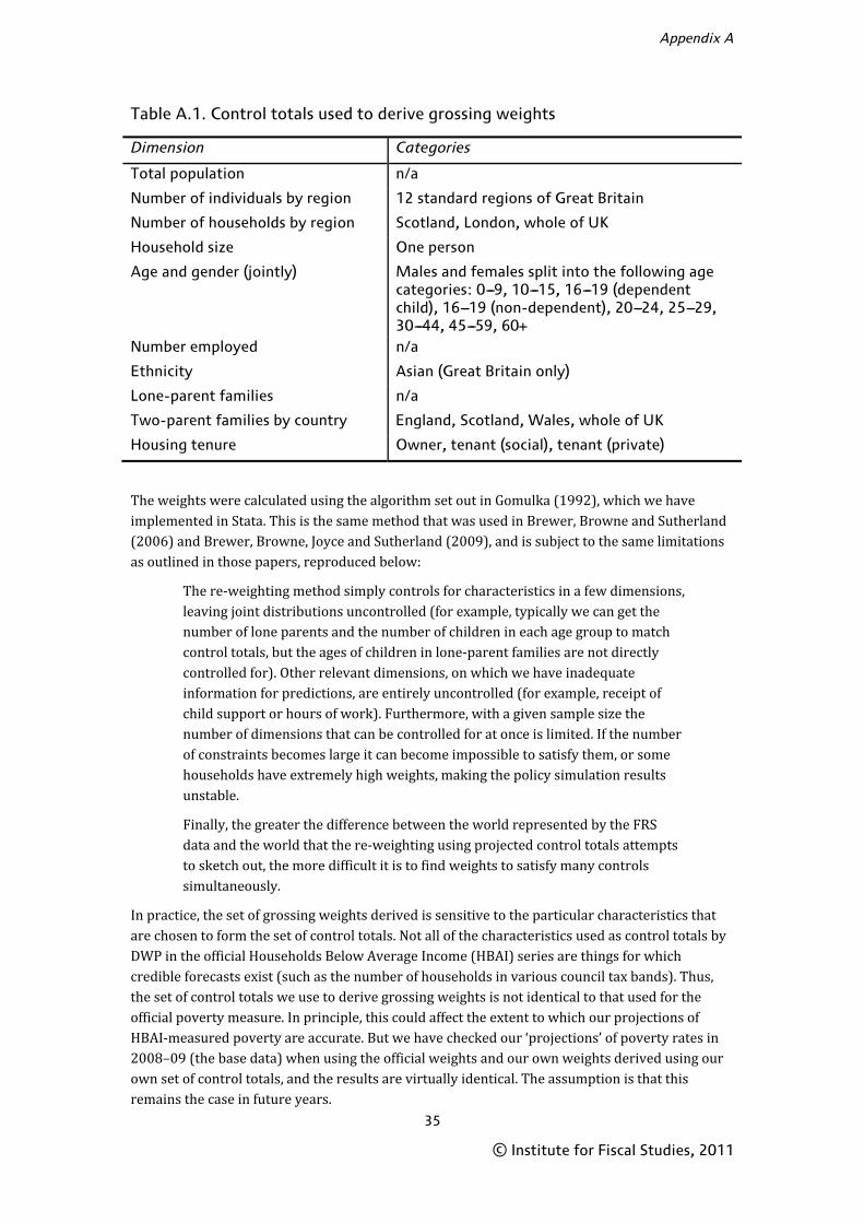
Appendix A
35
© Institute for Fiscal Studies, 2011
Table A.1. Control totals used to derive grossing weights
Dimension Categories
Total population n/a
Number of individuals by region 12 standard regions of Great Britain
Number of households by region Scotland, London, whole of UK
Household size One person
Age and gender (jointly) Males and females split into the following age categories: 0---9, 10---15, 16---19 (dependent child), 16---19 (non-dependent), 20---24, 25---29, 30---44, 45---59, 60+
Number employed n/a
Ethnicity Asian (Great Britain only)
Lone-parent families n/a
Two-parent families by country England, Scotland, Wales, whole of UK
Housing tenure Owner, tenant (social), tenant (private)
The weights were calculated using the algorithm set out in Gomulka (1992), which we have implemented in Stata. This is the same method that was used in Brewer, Browne and Sutherland (2006) and Brewer, Browne, Joyce and Sutherland (2009), and is subject to the same limitations as outlined in those papers, reproduced below:
The re-weighting method simply controls for characteristics in a few dimensions, leaving joint distributions uncontrolled (for example, typically we can get the number of lone parents and the number of children in each age group to match control totals, but the ages of children in lone-parent families are not directly controlled for). Other relevant dimensions, on which we have inadequate information for predictions, are entirely uncontrolled (for example, receipt of child support or hours of work). Furthermore, with a given sample size the number of dimensions that can be controlled for at once is limited. If the number of constraints becomes large it can become impossible to satisfy them, or some households have extremely high weights, making the policy simulation results unstable.
Finally, the greater the difference between the world represented by the FRS data and the world that the re-weighting using projected control totals attempts to sketch out, the more difficult it is to find weights to satisfy many controls simultaneously.
In practice, the set of grossing weights derived is sensitive to the particular characteristics that are chosen to form the set of control totals. Not all of the characteristics used as control totals by DWP in the official Households Below Average Income (HBAI) series are things for which credible forecasts exist (such as the number of households in various council tax bands). Thus, the set of control totals we use to derive grossing weights is not identical to that used for the official poverty measure. In principle, this could affect the extent to which our projections of HBAI-measured poverty are accurate. But we have checked our ‘projections’ of poverty rates in 2008–09 (the base data) when using the official weights and our own weights derived using our own set of control totals, and the results are virtually identical. The assumption is that this remains the case in future years.

Child and working-age poverty from 2010 to 2020
36
© Institute for Fiscal Studies, 2011
Simulating future tax liabilities and benefit and tax credit receipts
Using the IFS microsimulation model, TAXBEN, we can calculate the benefits and tax credits individuals and households are entitled to, and the taxes they are liable to pay, under hypothetical tax and benefit systems. Hence, using the current default rules for annually uprating tax thresholds and benefit and tax credit amounts, and taking account of preannounced direct tax and benefit reforms that are due to be implemented, we can simulate net household incomes in future years according to what the tax and benefit system will look like in those future years under current policies. (The uprating rules we use are given in Table A.2; we use the OBR forecasts of CPI inflation, RPI inflation and average earnings growth published alongside Budget 2011 and reproduced in Table A.3.)
Table A.2. Default uprating rules under current policies
Rule What it’s used to uprate
In line with RPI War pensions Scholarship income Income from government training schemes Allowances paid other than from spouse Council tax
In line with nominal earnings Water and sewerage rates Private pensions income Employment income Self-employment income Maintenance payments Allowances from absent spouse
In line with nominal GDP Imputed capital from savings, annuities, property, stocks and shares, and bonds
In line with RPI to previous September, rounded to nearest pound
National Insurance upper earnings limit
In line with RPI to previous September, increase rounded up to nearest £10
Income tax personal allowances Income tax married couple’s allowances
In line with RPI to previous September, increase rounded up to nearest £100
Income tax bands Threshold for withdrawal of older person’s income tax allowances
In line with CPI to previous September, rounded to nearest 5p
Child Benefit Severely disabled premiums on Income Support and Housing Benefit Incapacity Benefit Carer’s Allowance Disability Living Allowance Attendance Allowance Severe Disablement Allowance Local Housing Allowance rates (from April 2013)a Most Income Support rates Most Housing Benefit applicable amounts Non-dependant deductions for Income Support, Housing Benefit and Second Adult Council Tax Rebate

Appendix A
37
© Institute for Fiscal Studies, 2011
Table A.2 continued
Rule What it’s used to uprate
In line with CPI to previous September, rounded to nearest £5
Per-child element of Child Tax Credit Disabled and severely disabled elements of Child Tax Credit First tax credit threshold for those not entitled to Working Tax Credit All Working Tax Credit amounts
In line with CPI to previous September, rounded to nearest £1
Thresholds for non-dependant deductions for Income Support, Housing Benefit and Second Adult Council Tax Rebate National Insurance primary threshold
Increased by the maximum of average earnings index growth to previous September, CPI inflation to previous September, and 2.5%, rounded to nearest 5p
Basic State Pension Pension Credit guarantee amounts
Frozen Winter Fuel Payments to pensioners Income Support and Housing Benefit disregards Family element of Child Tax Credit First tax credit threshold National Local Housing Allowance caps
a. Before April 2013, Local Housing Allowance rates will continue to rise in line with rents.
Table A.3. OBR forecasts
2010 2011 2012 2013 2014 2015
CPI to previous September
3.1% 4.3% 2.3% 2.0% 2.0% 2.0%
RPI to previous September
4.6% 5.2% 3.4% 3.5% 3.6% 3.8%
Rossi to previous September
4.8% 5.4% 2.6% 2.7% 2.9% 2.9%
Nominal earnings growth
1.7% 2.0% 2.2% 3.8% 4.3% 4.5%
Nominal GDP growth
4.9% 4.8% 5.2% 5.7% 5.6% 5.6%
Source: Tables 1.1 and 4.3 of Office for Budget Responsibility (2011a). Rossi forecast published separately by the OBR at authors’ request; see http://budgetresponsibility.independent.gov.uk/wordpress/docs/ROSSI.pdf.
Child and working-age poverty from 2010 to 2020
38
© Institute for Fiscal Studies, 2011
However, an adjustment needs to be made to account for the fact that not everyone who is entitled to benefits and tax credits will claim them. Some households may be unaware of their entitlement, or find it too time-consuming to claim, or find claiming means-tested benefits stigmatising, or dislike the uncertainty around over- or under-payments that surrounds tax credit receipt.
We could use take-up rates based on administrative data to withdraw means-tested benefits and tax credits randomly from the appropriate fraction of eligible recipients. However, estimates of the take-up rates of benefits and tax credits from the FRS tend to be lower than those based on administrative data, even when allowance is made for the less-than-full coverage of the FRS (i.e. it omits people not in private households).23 This suggests that there is misreporting of means-tested benefit and tax credit income in the FRS (specifically, under-reporting). Since we are forecasting poverty as it is officially measured (i.e. using the FRS), we want to account for this.
Having obtained our simulated net incomes from TAXBEN, we therefore do the following. If someone is eligible for a benefit or tax credit in the 2008–09 base data, as simulated by TAXBEN, but they did not report receiving it in the FRS, then we assume that they will still not report taking up the benefit or tax credit in future years. (The implicit assumption is that the accuracy with which the FRS records benefit and tax credit receipt remains constant.) For those who were not eligible in the base data but are simulated by TAXBEN as becoming eligible in future years, we instead use administrative data on the take-up rates of different benefits and tax credits, disaggregated by various subgroups. We randomise take-up among these people, with the probability of take-up being equal to the caseload take-up rate from administrative data for that benefit or tax credit for the relevant subgroup. The latest take-up data for benefits come from DWP and are for 2008–09;24 the latest take-up data for tax credits come from HMRC and are for 2007–08.25
Note that Child Benefit will effectively become means-tested in January 2013, as the government plans to remove it from families containing a higher-rate taxpayer. However, this ‘means test’ will operate through the tax system: higher-rate taxpayers will be expected to declare the fact that they are higher-rate taxpayers so that their family does not receive Child Benefit. Hence, this reform has no impact on our assumption about the take-up of Child Benefit among those entitled (we continue to assume full take-up).
Since we do not know what the take-up rates of Universal Credit will be (nor how well its receipt will be recorded in the FRS), we need to make an assumption. We assume that those who are observed in our base data (from 2008–09) claiming a means-tested benefit or tax credit would continue to claim Universal Credit if they were eligible. For those who we predict will be entitled to Universal Credit but were not entitled to any means-tested benefits and tax credits in 2008–09, we assume that the take-up rate is the same as it currently is for the family element of the Child Tax Credit for those with children, and the same as for Working Tax Credit for those without children. We assume that those who do not take up any of their means-tested benefit entitlements continue to not claim Universal Credit. We also model variants where the observed take-up of Universal Credit is higher than this, which we might expect since Universal Credit, as an integrated benefit, is likely to be easier and less confusing to claim.
23 See appendix C in Brewer, Muriel, Phillips and Sibieta (2008). 24 See Department for Work and Pensions (2010b). 25 See HM Revenue and Customs (2010).

Appendix A
39
© Institute for Fiscal Studies, 2011
The poor are more likely to be eligible for substantial amounts of such benefits, so one might expect that they lose the most from lower take-up. Hence, absolute poverty projections will tend to be biased upwards if take-up is under-estimated, and vice versa. For relative poverty projections, the direction of bias from under- or over-estimating take-up is ambiguous because those with the lowest entitlements may be the most likely not to claim, and these are more likely to be households with an income around the median. Hence, lower take-up can in principle reduce relative poverty by reducing the median income (and hence the poverty line) by more than it reduces the incomes of low-income families.
For the benefit of analysts and modellers (or anyone interested in the extent to which non-take-up hinders efforts to reduce poverty), we provide the results obtained (for 2015–16) under a full-take-up scenario in Appendix B.
Creating the HBAI definition of income
Finally, we need to create a measure of disposable income that is as close as possible to that used when calculating official poverty statistics (the precise definition is given in Department for Work and Pensions (2010a)). To construct something broadly equivalent to this, we add together various sources of private (i.e. pre-transfer) income, subtract estimated tax liabilities, add estimated receipt of benefits and tax credits, and then subtract various ‘deductions’ from income. Table A.4 gives details of the various components of income.
Data on the deductions are partly derived from outputs from TAXBEN (e.g. council tax and contributions to a private pension) and partly taken from the official HBAI data set (because this is based on the FRS, we are able to merge the official HBAI data set with the data set produced by TAXBEN). We assume that this latter set of deductions (housing costs, child support paid for non-resident children, and financial support given by parents to children who are students living away from home) increase over time in line with average earnings.
Table A.4. Creating the HBAI definition of BHC income from TAXBEN
These are added together:
Gross employment income
Gross self-employment income
Imputed income from company cars and other benefits in kind
Free school meals
Savings income
Pensions income
Income from property
Any other unearned income
Maintenance payments from absent spouse
Benefits
These are subtracted: Expenses incurred in the course of employment
Self-employment net losses
Direct taxes
Council tax
Contributions to personal pensions
Maintenance payments made
Parental contributions to students

Child and working-age poverty from 2010 to 2020
40
© Institute for Fiscal Studies, 2011
We can then create a measure of household equivalised income, by summing this final measure of disposable income across all members of a household and multiplying by various factors to take account of household size and structure according to the modified OECD equivalence scale.26
A.2 Further modelling details
Harmonising TAXBEN-simulated incomes with HBAI-measured incomes
As noted in Brewer, Browne, Joyce and Sutherland (2009), the income distribution simulated by TAXBEN is not identical to the income distribution measured officially by HBAI, even though both use the same underlying FRS data. With no kind of adjustment to account for this, it is therefore likely that projections of future income distributions using TAXBEN would not accord with the actual income distribution in those future years as measured by HBAI (even if all our assumptions about policy, demographics and the macroeconomy turned out to be correct).
It is not surprising that there is some discrepancy between TAXBEN-simulated incomes and HBAI-measured incomes, for the following reasons:
• TAXBEN estimates income tax and National Insurance (NI) liabilities on the basis of relevant characteristics as measured by the FRS, whereas the HBAI series uses self-reported payments of direct taxes in the FRS. Inaccuracies in estimating income tax and NI liabilities, or inaccuracies in the information in the FRS on income tax and NI actually paid, will therefore lead to discrepancies.
• Similarly, TAXBEN estimates entitlements to means-tested benefits and tax credits, whereas the HBAI series uses self-reported receipts. Although, as described in Section A.1, we adjust for non-take-up, this adjustment cannot perfectly harmonise benefit and tax credit receipt in our simulated income distribution and the HBAI-measured distribution. Any inaccuracies in the FRS on the amounts of means-tested benefits and tax credits actually received among those who say that they receive some, or inaccuracies in estimating entitlements to means-tested benefits and tax credits in TAXBEN, will lead to discrepancies.
To account for these discrepancies, we check our TAXBEN-simulated incomes for each household in our 2008–09 base data against the 2008–09 HBAI-measured income for that household. We derive an additive correction term for each household such that, after the correction is applied, its 2008–09 TAXBEN-simulated income is identical to the income recorded in HBAI. We then use the same real-terms corrections for each household when projecting poverty in future years. Clearly, the extent to which TAXBEN-simulated and HBAI-measured incomes differ may not stay constant in real terms over time – it is likely, for example, that the discrepancy is a complicated function of the tax and benefit system and/or levels of earnings. But it is not clear what direction of bias (if any) this would lead to, in terms of projecting poverty rates, and it is highly likely that making an adjustment based on the discrepancy in the base year enables more accurate projections than making no adjustment at all. For the benefit of analysts and modellers, we provide the results obtained (for 2015–16) without applying any such correction in Appendix B.
26 See appendix 2 of Department for Work and Pensions (2011) for details of this equivalence scale.

Appendix A
41
© Institute for Fiscal Studies, 2011
Modelling rises in the state pension age
Between April 2010 and March 2016, the age at which women become entitled to the State Pension is rising by one month every two months from its pre-2010 level of 60, and will increase to 65 by November 2018. The state pension age will rise from 65 to 66 for both men and women between December 2018 and April 2020. This changes the sample of people who are of working age, which is clearly important when forecasting working-age poverty. But it also has implications for household incomes.
It is straightforward to model the direct impact on incomes of increasing the state pension age (SPA) in TAXBEN. But a couple of other issues remain. First, the maximum age at which individuals can receive Incapacity Benefit or Employment and Support Allowance (IB/ESA) is being raised as well, so that it remains in line with the SPA.27 We only observe entitlement to IB/ESA in the 2008–09 base data for those who were of eligible age in that year (i.e. women aged under 60 or men aged under 65). Thus, we have to estimate the probability of entitlement in future years for women aged between 60 and 65 and men aged 65. We estimate these probabilities from the sample of 58- and 59-year-old women and 63- and 64-year-old men in the base data by probit regression.28 The predictors we use are education, council tax band, region, housing tenure, partnership status, employment status of the partner (if applicable) and local authority disability status. We use these to generate predicted entitlement probabilities, and we randomise entitlements for the relevant individuals using those probabilities (the probabilities average about 10% for the relevant women and 15% for the relevant men).
A second issue is that households that include 60- to 65-year-old women and 65-year-old men in the future may look different from the corresponding households in 2008–09 (our base data), because these individuals (or other members of their household) may respond to whether or not they are entitled to the State Pension by changing their labour supply. Indeed, the age profile of employment probabilities exhibits a clear discontinuity at the SPA.29 Ignoring this issue would be very likely to lead to under-estimates of the incomes of those affected.
We estimate an equation linking work status (employed/not employed) for women aged 51 to 65 and men aged 56 to 65 to a number of predictors by probit regression. The predictors are education, region, housing tenure, council tax band, local authority disability status, entitlement to Disability Living Allowance, a cubic in age and an indicator variable for being below the SPA. We do this separately for single women, single men, men in couples and women in couples (for those in couples, we also include an indicator variable for whether or not the partner works). Having estimated this equation, we generate predicted employment probabilities for those not below SPA in the scenario where they are below SPA. Aggregating these predicted probabilities gives the predicted proportion of those directly affected by the SPA change who will be in work after that change. We then identify those affected individuals who are not working in the base data who have the highest predicted probabilities of being in work when below SPA (the most ‘marginal’ individuals), with the number we identify being calibrated so as to match our aggregate employment prediction (this involves increasing the employment rate by about 8 percentage points for the affected women and about 20 percentage points for the affected men). We then allocate these people gross earnings and a weekly number of hours worked. We do this
27 Similarly, the minimum age at which individuals can claim Attendance Allowance is rising. The direct impact of this is straightforward to model, by removing entitlement to Attendance Allowance from all individuals of the relevant age. 28 Note that there is not a discernible age profile in entitlement probabilities for women in their mid to late 50s. Thus, it seems reasonable to estimate entitlement probabilities using these control groups. 29 See, for example, figure 4.9 in Office for National Statistics (2009b).

Child and working-age poverty from 2010 to 2020
42
© Institute for Fiscal Studies, 2011
using nearest-neighbour propensity score matching, with those just below SPA in the base data being the control group (again, separately for single women, single men and for people in couples).30 Propensity scores are estimated by probit regression using an equation linking SPA status (above/below SPA) to the same set of predictors as in the employment equation above (but excluding the cubic in age).
There are some implicit assumptions here. First, there are no anticipation effects or dynamic effects on employment of raising the SPA: increasing the state pension age does not affect the employment probabilities of those below the original SPA or of those above the new SPA. Second, employment responses come only through the individuals directly affected by the SPA change, rather than through other members of their household. In practice, the husbands of those affected might also respond by retiring later (Banks, Blundell and Casanova, 2007). Third, the reason why there is a discontinuity in the age profile of employment probabilities at state pension age is because of the SPA itself, rather than some other factor. If this is not true, the actual behavioural response may be smaller.
Note that the OBR’s total employment forecasts, which we make use of, will already have accounted for the rise in SPA. Therefore, this adjustment does not affect our assumption about total employment: it simply affects our implicit assumption about the composition of the working population (most directly, with respect to age), because we reweight the data (see Section A.1) after modelling this behavioural response.
Having allocated the additional IB/ESA entitlements and gross earnings, we run the modified base data through TAXBEN in the normal way.
A.3 Accounting for welfare reforms that are more difficult to model precisely
The government has announced various direct tax and benefit reforms that are due to be implemented by 2020. Many of them simply involve changing the values of basic parameters of the tax and benefit system, such as the income tax personal allowance or Child Tax Credit amounts. These reforms can be straightforwardly modelled using TAXBEN. But some of the reforms are more difficult to model precisely, because their impact on particular families will depend upon characteristics of those families that are not perfectly measured in the FRS data. For example, the impact of migrating Incapacity Benefit (IB) claimants onto Employment and Support Allowance (ESA) will depend on who fails the medical test in ESA, which we cannot predict at the individual level. In its assessment of the distributional impact of tax and benefit changes, the Treasury did not include these hard-to-model reforms, and as a result provided an assessment of the distributional impact of only 30% (in revenue terms) of the direct tax and benefit reforms due to be implemented by 2012.31 But these hard-to-model reforms (all of which save the government money) have the potential to affect significantly assessments of the likely path of poverty in the near future. Therefore, in this work, we do attempt to account for those reforms that we judge can be modelled in a reasonably precise way, such that modelling them is very likely to lead to more accurate conclusions about poverty than ignoring them entirely. Below, we outline the policy changes that we take account of even though they cannot be
30 This seems reasonable as there is not a discernible age profile in earnings or hours worked among workers just below SPA. 31 See IFS evidence submitted to the Treasury Select Committee after the 2010 Spending Review at http://www.publications.parliament.uk/pa/cm201011/cmselect/cmtreasy/544/544pwe09.htm.
Appendix A
43
© Institute for Fiscal Studies, 2011
straightforwardly modelled using TAXBEN. (Note that most of these reforms are due to be implemented in 2013 or later: Local Housing Allowance reforms are the only ones that can have any impact on our poverty projections up to and including 2012.) First, we provide a full list of the future reforms that we model.
All the reforms that we model
Benefits and tax credits
• Uprate all benefits and tax credits with CPI from April 2011.
• Increase the child element of Child Tax Credit by £180 above indexation in April 2011 and £110 above indexation in April 2012.
• Increase the first and second tax credit taper rates to 41% in April 2011.
• Remove the baby element of Child Tax Credit in April 2011.
• Cancel the planned Child Tax Credit supplement for children aged 1 and 2 in April 2012.
• Taper the family element of Child Tax Credit immediately after the child element is withdrawn from April 2012.
• Remove the 50-plus element of Working Tax Credit in April 2012.
• Increase the Working Tax Credit working hours requirement for couples with children from 16 to 24 hours in April 2012.
• Reduce the proportion of costs covered by the childcare element of Working Tax Credit from 80% to 70% in April 2011.
• Freeze the basic and 30-hour elements of Working Tax Credit at 2010–11 rates from 2011–12 to 2013–14 inclusive.
• Freeze Child Benefit at 2010–11 rates from 2011–12 to 2013–14 inclusive.
• Remove Child Benefit from families containing a higher-rate taxpayer in January 2013.
• Uprate the Basic State Pension by the maximum of CPI inflation, earnings growth and 2.5% from April 2012, and uprate with RPI inflation in April 2011.
• Increase minimum guarantee for Pension Credit by the cash increase in Basic State Pension in April 2011.
• Freeze maximum award of Savings Credit at 2010–11 rates from 2011–12 to 2014–15 inclusive.
• Time-limit contributory Employment and Support Allowance to one year from April 2012.
• Local Housing Allowance: remove the £15 excess that can be claimed above rent, set local reference rates at the 30th percentile of local rents rather than the median, cap all rates at the four-bedroom rate and introduce national caps on all local reference rates in April 2011 (new claimants) or January to December 2012 (existing claimants); increase the age below which single people can only claim the shared-room rate from 25 to 35 in April 2012; and change annual uprating of local reference rates to CPI from April 2013.
• Housing Benefit deductions for non-dependants uprated with CPI from April 2011 (previously frozen in nominal terms).

Child and working-age poverty from 2010 to 2020
44
© Institute for Fiscal Studies, 2011
• Reduce Housing Benefit awards for those of working age under-occupying social housing from April 2013.
• Reform eligibility assessment for Disability Living Allowance in April 2013.
• Cap total household benefit payments at the level of average earnings for working households from April 2013.
• Introduce Universal Credit from October 2013.
Personal taxes
• £1,000 cash increase to the personal allowance in April 2011.
• £2,500 reduction in basic-rate limit, upper earnings limit and upper profits limit in April 2011.
• Freeze higher-rate threshold in 2012–13 and keep upper earnings limit and upper profits limit aligned with higher-rate threshold.
• Increase primary threshold in 2011–12 by £21 above alignment with where the personal allowance would have been under previous government’s plans.
• Increase all National Insurance rates by 1 percentage point in April 2011.
• Uprate some direct tax thresholds in line with CPI from April 2012.
Other
• Cancel extension of free school meals to primary-school children with parents in receipt of Working Tax Credit with a gross income lower than the first tax credit threshold for those not entitled to Working Tax Credit from September 2010.
• Abolish Sure Start Maternity Grant for second and subsequent children in April 2011.
• Freeze council tax in England in 2011–12.
Reforms that are more difficult to model precisely
The rest of this section discusses some of the reforms that are more difficult to model exactly in TAXBEN.
Local Housing Allowance reforms
Local Housing Allowance (LHA) is Housing Benefit for private renters. A series of reforms are planned:
• From April 2011 (for new claimants) or January to December 2012 (for existing claimants),32 the maximum amount of LHA that someone can claim will be equal to their local reference rate or their rent (whichever is lower), rather than their local reference rate or their rent plus £15 per week; local reference rates will be set at the 30th percentile of local rents rather than the median (50th percentile); reference rates in every area will be capped at the four-bedroom rate; and no local reference rates will be able to exceed certain national caps (these will be £250 per week for the shared-room rate and the one-bedroom rate, £290 for the two-bedroom rate, £340 for the three-bedroom rate and £400 for the four-bedroom rate).
32 Existing claimants will not be affected by the changes until the anniversary of their LHA claim, when they will lose entitlement to the £15 excess, and they will not be affected by the other reforms until nine months after the anniversary of their claim. We can model this phase-in accurately, as we observe the date on which an LHA claim started in the FRS data.

Appendix A
45
© Institute for Fiscal Studies, 2011
• From April 2012, single people under the age of 35 will only be eligible for the shared-room rate (currently, the age threshold is 25).
• From April 2013, local reference rates will be uprated annually in line with the consumer price index (CPI), rather than with local rents.
Local reference rates are set within Broad Rental Market Areas (BRMAs). In the FRS data available to us, we do not observe which BRMA people are in. However, we do observe the local authority (LA) that they are in, and we are able to map BRMAs to LAs. Since we know current reference rates in each BRMA (and we also know what those rates would currently be if they were set at the 30th percentile of local rents, as will be the case from April 2011), we are able to model very precisely the impact of LHA reforms on anyone who lives in an LA that contains a single BRMA, since we know exactly how much LHA they should currently be receiving. This applies to 36% of LAs. In cases where there is more than one BRMA falling within an LA, we take the median of the BRMA rates in that LA. Clearly, this involves some loss of precision, but there is no reason to suspect that it biases poverty forecasts in a particular direction. Our judgement is that this is likely to lead to significantly more accurate modelling than ignoring these reforms entirely (which has been the approach taken by HM Treasury analysts).
Note that we do not account for possible effects of the LHA reforms on the general level of rents, or on the housing costs of particular individuals who might move to a property with a lower level of rent as a result of the reforms. By lowering household costs, such ‘second-round’ effects would tend to increase household incomes when measured after housing costs (AHC). But they could in principle decrease household incomes measured before housing costs (BHC) if a household moves to a home (as a result of the reforms) with a level of rent that is less than the Housing Benefit they were receiving previously: in that case, Housing Benefit would fall to the new rent level or below. Similarly, if tenants find that rents fall for a given quality of property because of the reform, then an apparent decline in income measured BHC might not be accompanied by a decline in living standards.
Making Housing Benefit awards reflect family size for working-age tenants in social housing from April 2013
From April 2013, those of working age in the social rented sector will have their Housing Benefit awards capped depending on their family size (rather than the size of their house). Therefore, those of working age in under-occupied social housing will lose some Housing Benefit. We can precisely identify who these people are in the data, and we know the amount the government expects to raise from this measure, so we can estimate the average loss among those who lose from the policy. We do not know the precise distribution of losses among the losers – in reality, some will lose more than the average and some less. But because we can precisely identify the people who will lose something, our judgement is that assuming a constant proportional loss of Housing Benefit among the losers is very likely to be preferable to ignoring the reform entirely.
Reform to Disability Living Allowance (DLA) in April 2013
The government plans to replace DLA with a benefit called Personal Independence Payment (PIP). Part of the change will mean a new assessment process to determine eligibility, and the government has said that it expects the numbers in receipt of PIP to be about 20% lower than the numbers receiving DLA, as a result. We therefore know the number of losers (20% of DLA recipients) and the number of gainers (none), and we know that those who lose will lose all of their DLA. Although we do not know which DLA recipients will lose, our judgement is that we have enough information about the distribution of losses that an attempt to model the policy will lead to more accurate conclusions than a decision to ignore it entirely. We therefore remove DLA

Child and working-age poverty from 2010 to 2020
46
© Institute for Fiscal Studies, 2011
from a random 20% subset of DLA recipients. The implicit assumption is that the probability of losing DLA entitlement as a result of these reforms is unrelated to household income. We assume that entitlements to PIP match existing entitlements to DLA for those who continue to receive DLA/PIP.
Shift from Incapacity Benefit to Employment and Support Allowance
Incapacity Benefit (IB) was closed to new claimants in October 2008 and those who would have claimed this benefit are instead claiming Employment and Support Allowance (ESA). Therefore, by 2010–11, anyone still on IB must have been claiming it for over a year. Hence, when simulating a population for 2010–11, we assume that those observed in our base data (from 2008–09) as having been on IB for less than a year will be claiming ESA rather than IB. Since there will have been some turnover in the population on disability benefits in the period from 2008–09 to 2010–11 (the DWP tabulation tool tells us that the number of individuals claiming long-term IB fell by 150,000 between 2008–09 and 2010–11), we also assume that 150,000 of those claiming long-term IB in our base data claim ESA instead by 2010–11.
We also need to take account of the fact that, between 2011–12 and 2014–15, existing claimants of IB will be reassessed to determine whether they are entitled to ESA and, if so, which level of the benefit they are entitled to.33 Evidence from the first pilot areas where individuals were reassessed (Aberdeen and Burnley) shows that 30% of those individuals were placed in the Support Group, 38% were placed in the Work-Related Activity Group and 32% were found to be fit for work and so lost entitlement to disability benefits.34 However, many new claimants of these benefits have successfully appealed against the initial decisions made at their Work Capability Assessment. Therefore, in both the case of new claimants claiming ESA and existing IB claimants being moved across to ESA, we assume that the proportion of successful appeals is the same for those who are transferred from IB to ESA as for new claimants, meaning that we assume 31% are placed in the Support Group, 43% in the Work-Related Activity Group and only 26% lose entitlement altogether. We assume that the rate of reassessment is constant (i.e. 25% of those on IB in 2010–11 are reassessed for ESA in each year between 2011–12 and 2014–15).
Universal Credit35
From April 2014, the government intends to stop new claims of out-of-work benefits, tax credits, Housing Benefit and Council Tax Benefit and make new claimants claim Universal Credit instead. Although the White Paper Universal Credit: Welfare that Works36 sets out most of the key details about Universal Credit, some important decisions have yet to be taken, meaning that we have had to make assumptions, both about the policy itself and its implementation:
• The government has not set out how it intends to replace the childcare element of the Working Tax Credit within Universal Credit. We assume that those who are entitled to Universal Credit still receive the same amount of support for childcare as they would have done under the tax credit system. Although there is no way in which the government could implement this within Universal Credit, the government has stated that it wishes to spend
33 There are two levels of entitlement to ESA, depending on whether individuals are placed into the Work-Related Activity Group or the Support Group. Members of the Work-Related Activity Group are expected to attend work-focused interviews designed to help them prepare for work. Those in the Support Group receive a higher level of benefit and are not expected to look for work. 34 See http://research.dwp.gov.uk/asd/asd1/adhoc_analysis/2011/ib_reassessment.pdf. 35 For more details, see Brewer, Browne and Jin (2011). 36 Department for Work and Pensions, 2010c.

Appendix A
47
© Institute for Fiscal Studies, 2011
approximately the same amount of money on childcare as it does under the current system, so this seems a neutral assumption.
• Similarly, the government has not said how it intends to replace support for mortgage interest provided through Income Support. Again, we assume that those entitled to Universal Credit receive the same amount of support for mortgage interest as they do under the current system.
• The government has not decided who will be entitled to the benefits-in-kind provided under the current system to those on out-of-work benefits (e.g. free school meals and free prescriptions). Although most of these are not included in the HBAI definition of income, the value of free school meals is, so an assumption has to be made. As in the previous two cases, we assume that families receive free school meals only if they would have been eligible under the pre-Universal-Credit tax and benefit system. Again, it is unlikely that this rule could be implemented in practice when Universal Credit is introduced but since the government wishes to spend around the same amount of money on passported benefits as at present, this seems a relatively neutral assumption to make. However, these assumptions are not trivial, and our results are likely to change once we have the government’s final decisions on these issues.
• We assume that those aged under 25 receive lower rates of benefit, as they do for Jobseeker’s Allowance at the moment.
• We assume that students are entitled only to those components of Universal Credit where they are entitled to the corresponding benefit under the current system; in other words, they are entitled to the child additions (since students can receive Child Tax Credit), but not (in general) to the personal amount or housing component.
• We assume that couples with one person above state pension age and one person below state pension age will have to claim Universal Credit, as the government announced during the committee stage of the Welfare Reform Bill 2011 (see House of Commons Library (2011)). We assume that a couple pensioner premium will still be paid to these families, much as in Jobseeker’s Allowance at the moment.
• We have to make assumptions about the speed at which families will be moved from the existing benefits and tax credits to Universal Credit. The government has said that existing claimants will gradually be moved across to Universal Credit between April 2014 and October 2017 but that there will be no cash losers at the point of transition. We have taken this to mean that no one will see a cash reduction in their benefit entitlement as they are transferred from the existing set of means-tested benefits and tax credits to Universal Credit but that this transitional protection may expire once a family’s circumstances change. We therefore allow some families that we calculate as being entitled to less in benefits once we have moved them across to Universal Credit to keep their previous level of entitlement. We also give some families in both 2014–15 and 2015–16 no transitional protection at all – these correspond to those whose transitional protection expires between 2014–15 and 2015–16, and new claimants of Universal Credit. We do not allow for any transitional protection to apply in 2020–21: this effectively assumes that no one is entitled to transitional protection at this point, either because their circumstances have changed sufficiently for it to expire or because cash increases in Universal Credit rates mean that they receive more in cash terms than they did at the point of transition. Table A.5 shows the proportion of families we assign to various states in our 2014–15 and 2015–16 simulated populations.
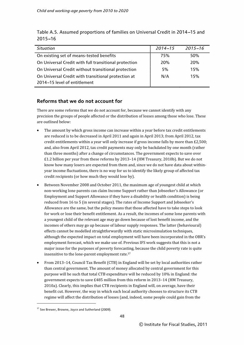
Child and working-age poverty from 2010 to 2020
48
© Institute for Fiscal Studies, 2011
Table A.5. Assumed proportions of families on Universal Credit in 2014---15 and 2015---16
Situation 2014---15 2015---16
On existing set of means-tested benefits 75% 50%
On Universal Credit with full transitional protection 20% 20%
On Universal Credit without transitional protection 5% 15%
On Universal Credit with transitional protection at 2014---15 level of entitlement
N/A 15%
Reforms that we do not account for
There are some reforms that we do not account for, because we cannot identify with any precision the groups of people affected or the distribution of losses among those who lose. These are outlined below:
• The amount by which gross income can increase within a year before tax credit entitlements are reduced is to be decreased in April 2011 and again in April 2013; from April 2012, tax credit entitlements within a year will only increase if gross income falls by more than £2,500; and, also from April 2012, tax credit payments may only be backdated by one month (rather than three months) after a change of circumstances. The government expects to save over £1.2 billion per year from these reforms by 2013–14 (HM Treasury, 2010b). But we do not know how many losers are expected from them and, since we do not have data about within-year income fluctuations, there is no way for us to identify the likely group of affected tax credit recipients (or how much they would lose by).
• Between November 2008 and October 2011, the maximum age of youngest child at which non-working lone parents can claim Income Support rather than Jobseeker’s Allowance (or Employment and Support Allowance if they have a disability or health condition) is being reduced from 16 to 5 (in several stages). The rates of Income Support and Jobseeker’s Allowance are the same, but the policy means that those affected have to take steps to look for work or lose their benefit entitlement. As a result, the incomes of some lone parents with a youngest child of the relevant age may go down because of lost benefit income, and the incomes of others may go up because of labour supply responses. The latter (behavioural) effects cannot be modelled straightforwardly with static microsimulation techniques, although the expected impact on total employment will have been incorporated in the OBR’s employment forecast, which we make use of. Previous IFS work suggests that this is not a major issue for the purposes of poverty forecasting, because the child poverty rate is quite insensitive to the lone-parent employment rate.37
• From 2013–14, Council Tax Benefit (CTB) in England will be set by local authorities rather than central government. The amount of money allocated by central government for this purpose will be such that total CTB expenditure will be reduced by 10% in England: the government expects to save £485 million from this reform in 2013–14 (HM Treasury, 2010a). Clearly, this implies that CTB recipients in England will, on average, have their benefit cut. However, the way in which each local authority chooses to structure its CTB regime will affect the distribution of losses (and, indeed, some people could gain from the
37 See Brewer, Browne, Joyce and Sutherland (2009).

Appendix A
49
© Institute for Fiscal Studies, 2011
reform). Since we have no idea how each local authority will design its CTB regime (or even which parameters of the regime it will have discretion over), we know nothing about the distribution of losses (and gains) from this reform, so there is no credible way of modelling its impact on poverty. We continue to ignore this reform when Universal Credit is introduced: we assume that there is a component in Universal Credit that is equal to a family’s council tax liability. This is the approach taken by DWP in the analysis of Universal Credit accompanying the White Paper and the Welfare Reform Bill.
Note that there are very important differences between simple distributional analyses of tax and benefit reforms and an analysis of the effect of those reforms on poverty. In the former case, all that is required is to get average losses correct within broadly defined subgroups (IFS researchers typically use decile groups – tenths of the population). But poverty rates are defined by the number of people whose income falls below a certain level. This means that the entire distribution of losses from a reform is of crucial importance in determining the impact on poverty. Take the reforms to gross income disregards in the tax credit system as an example. Since those individuals who receive large proportions of their income from tax credits are clustered in a few decile groups towards the bottom of the income distribution, the assumption of constant proportional losses among all tax credit recipients is likely to yield a reasonable approximation of the average loss by decile group. But the same is not true when projecting a poverty rate, because for that the entire distribution of losses matters crucially (and note that for relative poverty, effects of policies on the level of median income must be credibly taken into account).
Hence, most of the policies in the bullet points above have been modelled by IFS researchers when conducting distributional analysis by decile group,38 but we judge that they cannot be credibly modelled for the purposes of poverty forecasting.
All of the policies listed above that we are not modelling are welfare cuts. Hence, the direct impact of these reforms would be to reduce the incomes of some people on benefits. This would be likely to increase absolute poverty. The direct effect on relative poverty is ambiguous, because the cuts may also affect the level of median income and therefore the relative poverty line.
A.4 Uncertainties and limitations
This exercise is necessarily subject to much uncertainty. As always with survey data, there is likely to be sampling error in the FRS from year to year. This will affect the base data that underlie our projections and the future HBAI measures of poverty that we are trying to forecast. But there are other (probably greater) sources of uncertainty here.
First, there is naturally considerable uncertainty surrounding any demographic or macroeconomic forecasts such as those we make use of in producing these poverty projections. The current macroeconomic situation suggests that the degree of uncertainty surrounding some assumptions (such as employment rates and real earnings growth) is greater than normal. No projections can be immune from these uncertainties, although we do quantify the sensitivity of our results to key macroeconomic assumptions (see Chapter 4).
In addition, with the techniques employed here, we cannot directly account for behavioural responses to direct tax and benefit reforms (although we indirectly account for some such responses if they are already incorporated in the official forecasts of variables such as
38 See Browne and Levell (2010) and Browne (2010).
Child and working-age poverty from 2010 to 2020
50
© Institute for Fiscal Studies, 2011
employment and demographics that we make use of). Relevant kinds of behavioural responses include labour supply changes or fertility changes as a result of changes in state support for families with children (see Brewer, Ratcliffe and Smith (2011)). However, we do examine the sensitivity of our projections to potential labour supply responses from workless households as a result of the introduction of Universal Credit. We examine how poverty would be affected if various numbers of individuals in workless households whose financial incentive to work increased by the most were to move into paid work as a result. We measure the financial incentive to work using the participation tax rate (PTR), which gives the proportion of gross earnings that is lost in taxes or reduced benefit entitlements when an individual moves into paid work. We also examine a scenario where, in addition to this, 100,000 individuals who see their PTRs increase stop paid work. We use a methodology outlined in Brewer, Browne and Jin (2011) to estimate which individuals see the biggest reductions in their PTRs when Universal Credit is introduced, and to estimate how much current non-workers would earn were they to work.
Of course, our projections may turn out to differ from actual poverty rates because of new policies that are announced. The exercise here is not to predict future policy changes, but to produce our best estimate of what would happen if policy did not change.

51
© Institute for Fiscal Studies, 2011
Appendix B. Poverty projections under full take-up and without applying any ‘correction’ to simulated incomes
The purpose of the results in this appendix is primarily to illustrate the importance, when modelling poverty, of accounting for non-take-up of means-tested benefits and tax credits (see Section A.1) and of making some adjustment for the fact that tax and benefit microsimulation output does not perfectly replicate the survey data on which it is based (see Section A.2). We also demonstrate the effect of our reweighting to take account of demographic changes by showing how our results change when we use the original FRS survey weights. These adjustments are not included in the sensitivity analysis in Chapter 4, since in no circumstances do we think that ignoring non-take-up or the discrepancy between TAXBEN and HBAI-measured poverty approximates a realistic alternative ‘scenario’ for the path of poverty. Rather, this appendix is intended mostly for the benefit of analysts and modellers.
Tables B.1 and B.2 reiterate our 2015–16 central projection of relative and absolute BHC income poverty under current policies, and compare them with the projections obtained when:
a. applying no ‘correction’ to simulated incomes; b. assuming full take-up and applying no ‘correction’ to simulated incomes; c. using the original survey weights rather than the weights we calculate to match projected
control totals for the 2015–16 population.
Note that it makes little sense to consider the case where full take-up is assumed but the ‘correction’ to simulated incomes continues to be applied. This is because the necessary correction would itself be changed by the fact that full take-up is assumed (since this would change the discrepancies between TAXBEN-simulated income and HBAI-measured incomes in 2008–09, the base year), obscuring the effect of assuming full take-up.
Table B.1. Projections of relative BHC income poverty in 2015---16 when applying no corrections to simulated income, under full take-up and with original survey weights
Children Working-age adults without children
Median income (2010 prices)
Millions % Millions %
Baseline 2.9 22.2 4.0 15.9 £411 p.w.
a. No income correction 2.6 19.9 3.8 15.0 £416 p.w.
b. Full take-up and no income correction
2.2 16.4 3.4 13.2 £423 p.w.
c. With original survey weights 2.9 22.3 3.8 15.8 £417 p.w.
Source: Authors’ calculations based on Family Resources Survey, 2008---09, using TAXBEN and assumptions specified in the text.

Child and working-age poverty from 2010 to 2020
52
© Institute for Fiscal Studies, 2011
Table B.2. Projections of absolute BHC income poverty in 2015---16 when applying no corrections to simulated income, under full take-up and with original survey weights
Children Working-age adults without children
Millions % Millions %
Baseline 3.0 22.8 4.1 16.0
a. No income correction 2.6 19.4 3.7 14.7
b. Full take-up and no income correction
1.9 14.4 3.2 12.6
c. With original survey weights 2.8 22.0 3.8 15.7
Source: Authors’ calculations based on Family Resources Survey, 2008---09, using TAXBEN and assumptions specified in the text.

53
© In
stit
ute
for
Fisc
al S
tudi
es, 2
01
1
A
pp
end
ix C
. Po
vert
y p
roje
ctio
ns w
ith
out
th
e co
alit
ion
go
vern
men
t’s
tax
and
ben
efit
ref
orm
s
Tabl
e C
.1. P
roje
ctio
ns o
f re
lati
ve in
com
e po
vert
y in
the
UK
wit
hout
coa
litio
n go
vern
men
t’s
tax
and
bene
fit
refo
rms
C
hild
ren
W
orki
ng
-ag
e a
dul
ts
Wor
kin
g-a
ge
pare
nts
W
orki
ng
-ag
e a
dul
ts
wit
hou
t ch
ildre
n
Rea
l an
nua
l m
edia
n in
com
e g
row
th (
%)
M
illio
ns
%
Mill
ion
s %
M
illio
ns
%
Mill
ion
s %
In
com
es m
easu
red
bef
ore
ded
ucti
ng
hou
sin
g c
osts
B
HC
20
11
2.5
1
9.2
5
.7
15
.5
2.1
1
6.5
3
.6
15
.0
---3.0
20
12
2.5
1
8.8
5
.8
15
.5
2.1
1
6.3
3
.7
15
.1
---0.0
20
13
2.6
1
9.5
6
.0
15
.8
2.2
1
6.9
3
.8
15
.2
+0.7
20
14
2.7
2
0.3
6
.1
16
.0
2.3
1
7.4
3
.8
15
.2
+1.4
20
15
2.8
2
0.9
6
.2
16
.2
2.3
1
7.8
3
.9
15
.4
+0.8
20
20
3.0
2
2.8
7
.1
17
.3
2.5
1
9.1
4
.6
16
.4
+0.7
a
Inco
mes
mea
sure
d a
fter
ded
ucti
ng
hou
sin
g c
osts
A
HC
20
11
3.5
2
6.5
7
.6
20
.6
3.0
2
3.2
4
.6
19
.2
---3.0
20
12
3.4
2
6.0
7
.6
20
.4
3.0
2
2.9
4
.6
19
.0
+1.3
20
13
3.5
2
6.8
7
.7
20
.5
3.1
2
3.4
4
.7
18
.9
+1.8
20
14
3.7
2
7.8
7
.9
20
.6
3.1
2
4.0
4
.7
18
.9
+2.2
20
15
3.8
2
8.6
8
.0
20
.8
3.2
2
4.6
4
.8
18
.9
+1.8
20
20
4.1
3
0.9
8
.8
21
.4
3.4
2
6.0
5
.4
19
.3
+1.3
a
a. R
eal a
vera
ge a
nnua
l med
ian
inco
me
gro
wth
, 20
15
to
20
20
. N
ote
s: P
ove
rty
line
is 6
0% o
f m
edia
n in
com
e. Y
ears
ref
er t
o f
inan
cial
yea
rs.
Sour
ce:
Aut
hors
’ cal
cula
tio
ns b
ased
on
Fam
ily R
eso
urce
s Su
rvey
, 20
08
---09
, usi
ng T
AX
BE
N a
nd a
ssum
ptio
ns s
peci
fied
in t
he t
ext.
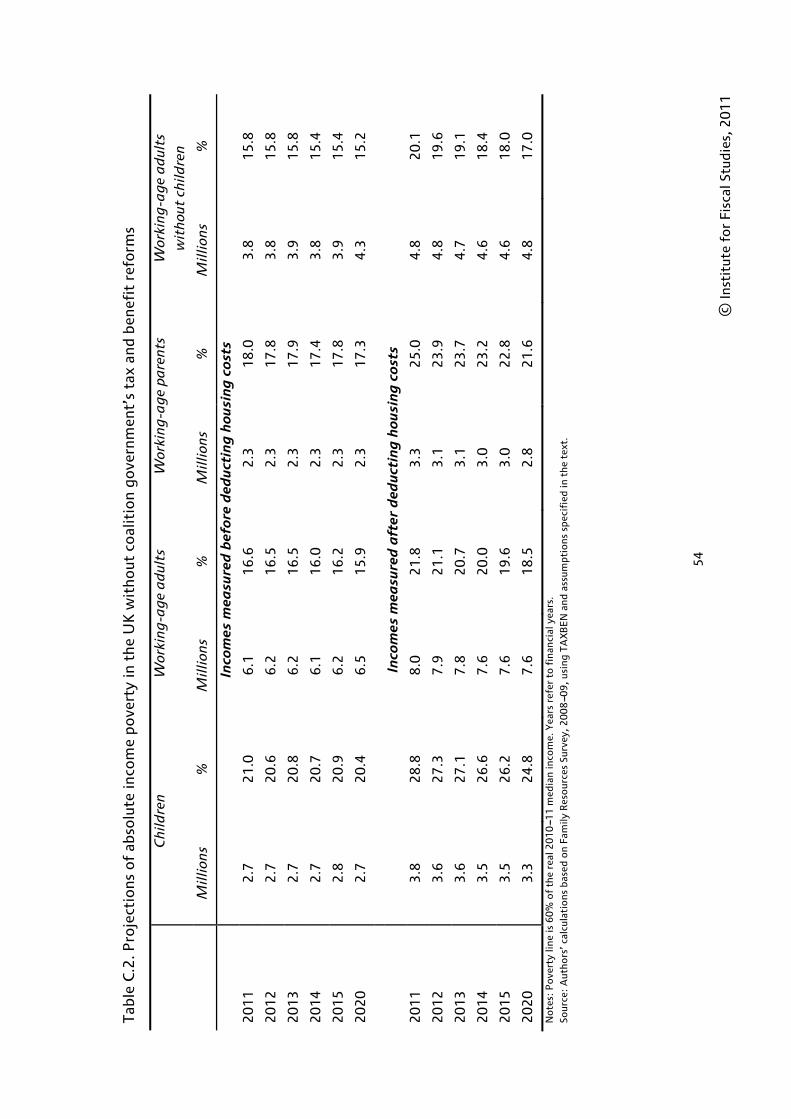
54
© In
stit
ute
for
Fisc
al S
tudi
es, 2
01
1
Tabl
e C
.2. P
roje
ctio
ns o
f ab
solu
te in
com
e po
vert
y in
the
UK
wit
hout
coa
litio
n go
vern
men
t’s
tax
and
bene
fit
refo
rms
C
hild
ren
W
orki
ng
-ag
e a
dul
ts
Wor
kin
g-a
ge
pare
nts
W
orki
ng
-ag
e a
dul
ts
wit
hou
t ch
ildre
n
M
illio
ns
%
Mill
ion
s %
M
illio
ns
%
Mill
ion
s %
In
com
es m
easu
red
bef
ore
ded
ucti
ng
hou
sin
g c
osts
20
11
2.7
2
1.0
6
.1
16
.6
2.3
1
8.0
3
.8
15
.8
20
12
2.7
2
0.6
6
.2
16
.5
2.3
1
7.8
3
.8
15
.8
20
13
2.7
2
0.8
6
.2
16
.5
2.3
1
7.9
3
.9
15
.8
20
14
2.7
2
0.7
6
.1
16
.0
2.3
1
7.4
3
.8
15
.4
20
15
2.8
2
0.9
6
.2
16
.2
2.3
1
7.8
3
.9
15
.4
20
20
2.7
2
0.4
6
.5
15
.9
2.3
1
7.3
4
.3
15
.2
In
com
es m
easu
red
aft
er d
educ
tin
g h
ousi
ng
cos
ts
20
11
3.8
2
8.8
8
.0
21
.8
3.3
2
5.0
4
.8
20
.1
20
12
3.6
2
7.3
7
.9
21
.1
3.1
2
3.9
4
.8
19
.6
20
13
3.6
2
7.1
7
.8
20
.7
3.1
2
3.7
4
.7
19
.1
20
14
3.5
2
6.6
7
.6
20
.0
3.0
2
3.2
4
.6
18
.4
20
15
3.5
2
6.2
7
.6
19
.6
3.0
2
2.8
4
.6
18
.0
20
20
3.3
2
4.8
7
.6
18
.5
2.8
2
1.6
4
.8
17
.0
Not
es:
Pov
erty
line
is 6
0%
of
the
real
20
10
---11
med
ian
inco
me.
Yea
rs r
efer
to
fina
ncia
l yea
rs.
Sour
ce:
Aut
hors
’ cal
cula
tio
ns b
ased
on
Fam
ily R
eso
urce
s Su
rvey
, 20
08
---09
, usi
ng T
AX
BE
N a
nd a
ssum
ptio
ns s
peci
fied
in t
he t
ext.

55
© In
stit
ute
for
Fisc
al S
tudi
es, 2
01
1
A
pp
end
ix D
. Po
vert
y ra
tes
usin
g 5
0%
an
d 7
0%
of
med
ian
inco
me
Tabl
e D
.1. P
roje
ctio
ns o
f re
lati
ve in
com
e po
vert
y in
the
UK
usi
ng p
over
ty li
ne o
f 50
% o
f m
edia
n in
com
e
No
tes:
Po
vert
y lin
e is
50%
of
med
ian
inco
me.
Yea
rs r
efer
to
fin
anci
al y
ears
. So
urce
: A
utho
rs’ c
alcu
lati
ons
bas
ed o
n Fa
mily
Res
our
ces
Surv
ey, 2
00
8---0
9, u
sing
TA
XB
EN
and
ass
umpt
ions
spe
cifi
ed in
the
tex
t.
C
hild
ren
W
orki
ng
-ag
e a
dul
ts
Wor
kin
g-a
ge
pare
nts
W
orki
ng
-ag
e a
dul
ts
wit
hou
t ch
ildre
n
M
illio
ns
%
Mill
ion
s %
M
illio
ns
%
Mill
ion
s %
In
com
es m
easu
red
bef
ore
ded
ucti
ng
hou
sin
g c
osts
20
10
1.3
9
.8
3.5
9
.5
1.2
9
.0
2.3
9
.8
20
11
1.3
9
.7
3.5
9
.6
1.2
9
.0
2.4
9
.9
20
12
1.3
1
0.1
3
.7
9.9
1
.2
9.5
2
.5
10
.2
20
13
1.5
1
1.1
4
.0
10
.5
1.3
1
0.2
2
.6
10
.6
20
14
1.5
1
1.5
4
.1
10
.6
1.4
1
0.5
2
.7
10
.7
20
15
1.5
1
1.2
4
.1
10
.6
1.4
1
0.3
2
.8
10
.8
20
20
1.6
1
2.4
4
.9
11
.9
1.4
1
0.8
3
.5
12
.4
In
com
es m
easu
red
aft
er d
educ
tin
g h
ousi
ng
cos
ts
20
10
2.2
1
6.8
5
.4
14
.9
2.0
1
5.4
3
.4
14
.6
20
11
2.2
1
6.6
5
.5
15
.0
2.0
1
5.4
3
.5
14
.7
20
12
2.3
1
7.5
5
.7
15
.2
2.1
1
6.1
3
.6
14
.7
20
13
2.5
1
8.8
5
.9
15
.7
2.2
1
7.1
3
.7
15
.0
20
14
2.5
1
9.2
5
.9
15
.6
2.2
1
7.2
3
.7
14
.7
20
15
2.5
1
9.1
6
.1
15
.8
2.3
1
7.2
3
.8
15
.0
20
20
2.8
2
1.3
7
.0
16
.9
2.4
1
8.5
4
.6
16
.2

56
© In
stit
ute
for
Fisc
al S
tudi
es, 2
01
1
Tabl
e D
.2. P
roje
ctio
ns o
f ab
solu
te in
com
e po
vert
y in
the
UK
usi
ng p
over
ty li
ne o
f 50
% o
f m
edia
n in
com
e
Not
es:
Pov
erty
line
is 5
0%
of
med
ian
inco
me
in 2
01
0---1
1. Y
ears
ref
er t
o fi
nanc
ial y
ears
. So
urce
: A
utho
rs’ c
alcu
lati
ons
bas
ed o
n Fa
mily
Res
our
ces
Surv
ey, 2
00
8---0
9, u
sing
TA
XB
EN
and
ass
umpt
ions
spe
cifi
ed in
the
tex
t.
C
hild
ren
W
orki
ng
-ag
e a
dul
ts
Wor
kin
g-a
ge
pare
nts
W
orki
ng
-ag
e a
dul
ts
wit
hou
t ch
ildre
n
M
illio
ns
%
Mill
ion
s %
M
illio
ns
%
Mill
ion
s %
In
com
es m
easu
red
bef
ore
ded
ucti
ng
hou
sin
g c
osts
20
10
1.3
9
.8
3.5
9
.5
1.2
9
.0
2.3
9
.8
20
11
1.4
1
0.4
3
.7
10
.1
1.2
9
.6
2.5
1
0.5
20
12
1.5
1
1.3
4
.0
10
.7
1.4
1
0.4
2
.6
10
.8
20
13
1.6
1
2.1
4
.2
11
.1
1.4
1
1.0
2
.8
11
.2
20
14
1.6
1
2.2
4
.2
11
.0
1.4
1
1.0
2
.8
11
.1
20
15
1.5
1
1.5
4
.1
10
.7
1.4
1
0.5
2
.8
10
.8
20
20
1.5
1
1.5
4
.7
11
.3
1.3
1
0.1
3
.5
12
.4
In
com
es m
easu
red
aft
er d
educ
tin
g h
ousi
ng
cos
ts
20
10
2.2
1
6.8
5
.4
14
.9
2.0
1
5.4
3
.4
14
.6
20
11
2.3
1
7.8
5
.8
15
.6
2.1
1
6.4
3
.6
15
.2
20
12
2.4
1
8.1
5
.8
15
.6
2.2
1
6.6
3
.7
15
.1
20
13
2.5
1
9.0
6
.0
16
.0
2.3
1
7.2
3
.8
15
.3
20
14
2.5
1
8.8
5
.9
15
.4
2.2
1
6.9
3
.7
14
.6
20
15
2.6
1
9.3
6
.1
15
.8
2.3
1
7.4
3
.8
15
.0
20
20
2.3
1
7.1
6
.1
14
.8
2.0
1
5.4
4
.1
14
.5

57
© In
stit
ute
for
Fisc
al S
tudi
es, 2
01
1
Tabl
e D
.3. P
roje
ctio
ns o
f re
lati
ve in
com
e po
vert
y in
the
UK
usi
ng p
over
ty li
ne o
f 70
% o
f m
edia
n in
com
e
No
tes:
Po
vert
y lin
e is
70%
of
med
ian
inco
me.
Yea
rs r
efer
to
fin
anci
al y
ears
. So
urce
: A
utho
rs’ c
alcu
lati
ons
bas
ed o
n Fa
mily
Res
our
ces
Surv
ey, 2
00
8---0
9, u
sing
TA
XB
EN
and
ass
umpt
ions
spe
cifi
ed in
the
tex
t.
C
hild
ren
W
orki
ng
-ag
e a
dul
ts
Wor
kin
g-a
ge
pare
nts
W
orki
ng
-ag
e a
dul
ts
wit
hou
t ch
ildre
n
M
illio
ns
%
Mill
ion
s %
M
illio
ns
%
Mill
ion
s %
In
com
es m
easu
red
bef
ore
ded
ucti
ng
hou
sin
g c
osts
20
10
4.0
3
0.5
7
.9
21
.8
3.3
2
5.4
4
.6
19
.8
20
11
4.0
3
0.5
8
.1
22
.0
3.3
2
5.7
4
.8
20
.0
20
12
4.0
3
0.6
8
.2
22
.0
3.4
2
5.7
4
.9
20
.1
20
13
4.2
3
2.1
8
.6
22
.7
3.5
2
6.8
5
.1
20
.6
20
14
4.3
3
2.8
8
.6
22
.6
3.5
2
7.1
5
.1
20
.3
20
15
4.4
3
3.5
8
.8
22
.9
3.6
2
7.5
5
.2
20
.5
20
20
4.7
3
5.2
9
.9
24
.1
3.7
2
8.6
6
.2
22
.0
In
com
es m
easu
red
aft
er d
educ
tin
g h
ousi
ng
cos
ts
20
10
4.8
3
6.8
9
.6
26
.3
4.1
3
1.4
5
.5
23
.5
20
11
4.8
3
7.0
9
.7
26
.4
4.1
3
1.6
5
.6
23
.6
20
12
4.9
3
7.0
9
.9
26
.5
4.2
3
2.1
5
.7
23
.5
20
13
5.0
3
8.4
1
0.2
2
6.9
4
.3
32
.9
5.9
2
3.8
20
14
5.1
3
8.7
1
0.2
2
6.8
4
.3
33
.0
5.9
2
3.5
20
15
5.2
3
9.2
1
0.4
2
7.0
4
.4
33
.3
6.1
2
3.8
20
20
5.5
4
0.8
1
1.4
2
7.7
4
.5
34
.4
6.9
2
4.6
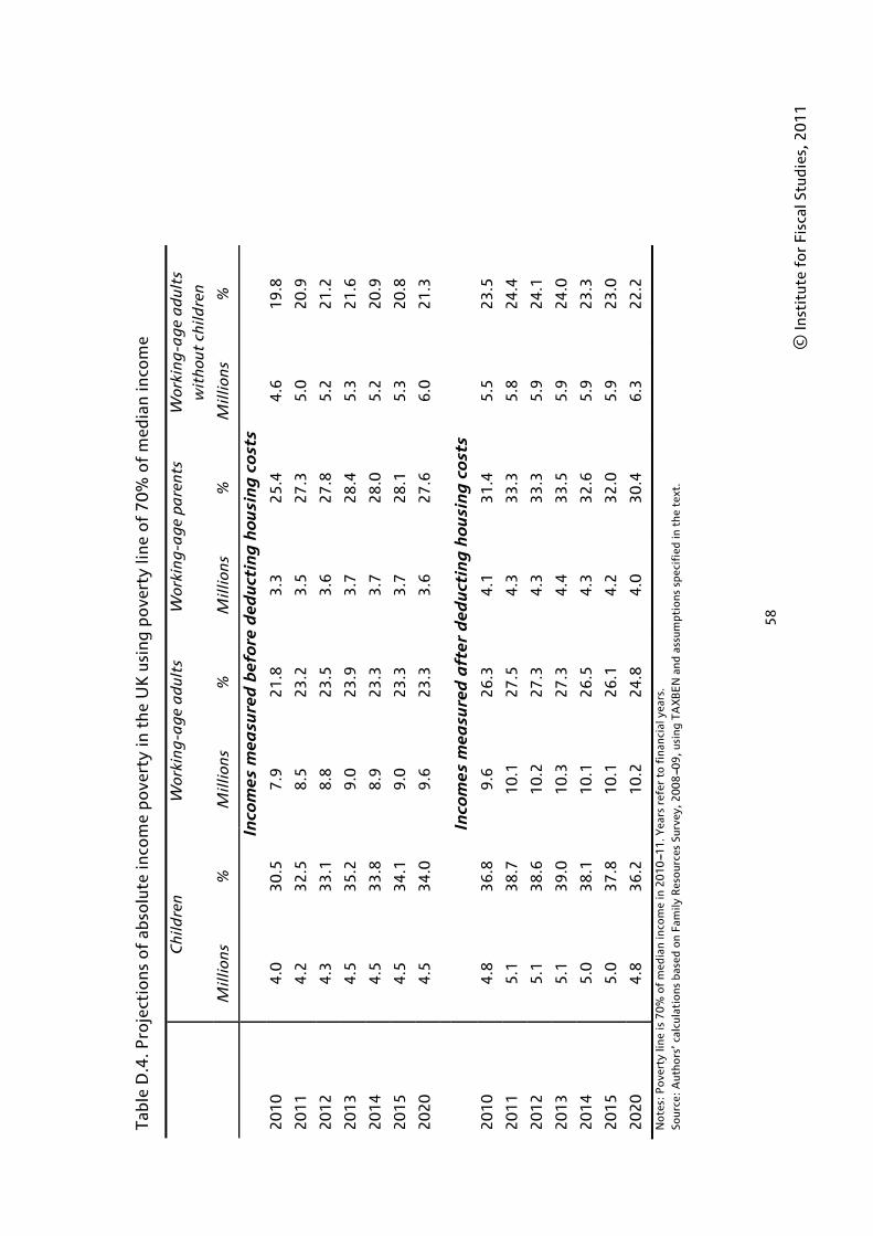
58
© In
stit
ute
for
Fisc
al S
tudi
es, 2
01
1
Tabl
e D
.4. P
roje
ctio
ns o
f ab
solu
te in
com
e po
vert
y in
the
UK
usi
ng p
over
ty li
ne o
f 70
% o
f m
edia
n in
com
e
Not
es:
Pov
erty
line
is 7
0%
of
med
ian
inco
me
in 2
01
0---1
1. Y
ears
ref
er t
o fi
nanc
ial y
ears
. So
urce
: A
utho
rs’ c
alcu
lati
ons
bas
ed o
n Fa
mily
Res
our
ces
Surv
ey, 2
00
8---0
9, u
sing
TA
XB
EN
and
ass
umpt
ions
spe
cifi
ed in
the
tex
t.
C
hild
ren
W
orki
ng
-ag
e a
dul
ts
Wor
kin
g-a
ge
pare
nts
W
orki
ng
-ag
e a
dul
ts
wit
hou
t ch
ildre
n
M
illio
ns
%
Mill
ion
s %
M
illio
ns
%
Mill
ion
s %
In
com
es m
easu
red
bef
ore
ded
ucti
ng
hou
sin
g c
osts
20
10
4.0
3
0.5
7
.9
21
.8
3.3
2
5.4
4
.6
19
.8
20
11
4.2
3
2.5
8
.5
23
.2
3.5
2
7.3
5
.0
20
.9
20
12
4.3
3
3.1
8
.8
23
.5
3.6
2
7.8
5
.2
21
.2
20
13
4.5
3
5.2
9
.0
23
.9
3.7
2
8.4
5
.3
21
.6
20
14
4.5
3
3.8
8
.9
23
.3
3.7
2
8.0
5
.2
20
.9
20
15
4.5
3
4.1
9
.0
23
.3
3.7
2
8.1
5
.3
20
.8
20
20
4.5
3
4.0
9
.6
23
.3
3.6
2
7.6
6
.0
21
.3
In
com
es m
easu
red
aft
er d
educ
tin
g h
ousi
ng
cos
ts
20
10
4.8
3
6.8
9
.6
26
.3
4.1
3
1.4
5
.5
23
.5
20
11
5.1
3
8.7
1
0.1
2
7.5
4
.3
33
.3
5.8
2
4.4
20
12
5.1
3
8.6
1
0.2
2
7.3
4
.3
33
.3
5.9
2
4.1
20
13
5.1
3
9.0
1
0.3
2
7.3
4
.4
33
.5
5.9
2
4.0
20
14
5.0
3
8.1
1
0.1
2
6.5
4
.3
32
.6
5.9
2
3.3
20
15
5.0
3
7.8
1
0.1
2
6.1
4
.2
32
.0
5.9
2
3.0
20
20
4.8
3
6.2
1
0.2
2
4.8
4
.0
30
.4
6.3
2
2.2

59
© Institute for Fiscal Studies, 2011
References
Bank of England (2011), Inflation Report May 2011 (http://www.bankofengland.co.uk/publications/inflationreport/ir11may.pdf).
Banks, J., Blundell, R. and Casanova, M. (2007), ‘The dynamics of retirement behavior in couples: reduced-form evidence from England and the US’, University College London, mimeo (http://m.rand.org/content/dam/rand/www/external/labor/aging/rsi/rsi_papers/2008/banks1.pdf).
Brewer, M., Browne, J., Emmerson, C., Goodman, A., Muriel, A. and Tetlow, G. (2007), Pensioner Poverty over the Next Decade: What Role for Tax and Benefit Reform?, Commentary 103, London: Institute for Fiscal Studies (http://www.ifs.org.uk/publications/3991).
Brewer, M., Browne, J. and Jin, W. (2011), ‘Universal Credit: a preliminary analysis’, IFS Briefing Note 116 (http://www.ifs.org.uk/publications/5415).
Brewer, M., Browne, J., Joyce, R. and Sibieta, L. (2010), ‘Child poverty in the UK since 1998–99: lessons from the past decade’, Institute for Fiscal Studies, Working Paper 10/23 (http://www.ifs.org.uk/publications/5303).
Brewer, M., Browne, J., Joyce, R. and Sutherland, H. (2009), Micro-Simulating Child Poverty in 2010 and 2020, Commentary 108, London: Institute for Fiscal Studies (http://www.ifs.org.uk/publications/4434).
Brewer, M., Browne, J. and Sutherland, H. (2006), Micro-Simulating Child Poverty in 2010 and 2020, York: Joseph Rowntree Foundation (http://www.ifs.org.uk/publications/3656).
Brewer, M. and Joyce, R. (2010), Child and Working-Age Poverty from 2010 to 2013, IFS Briefing Note 115 (http://www.ifs.org.uk/publications/5373).
Brewer, M., May, R. and Phillips, D. (2009), Taxes, Benefits and the National Minimum Wage, London: Low Pay Commission (http://www.lowpay.gov.uk/lowpay/research/pdf/FromLPC_Document_Feb.pdf).
Brewer, M., Muriel, A., Phillips, D. and Sibieta, L. (2008), Poverty and Inequality in the UK: 2008, Commentary 105, London: Institute for Fiscal Studies (http://www.ifs.org.uk/publications/4258).
Brewer, M., Muriel, A., Phillips, D. and Sibieta, L. (2009), Poverty and Inequality in the UK: 2009, Commentary 109, London: Institute for Fiscal Studies (http://www.ifs.org.uk/publications/4524).
Brewer, M., Ratcliffe, A. and Smith, S. (2011), ‘Does welfare reform affect fertility? Evidence from the UK’, Journal of Population Economics, forthcoming; an earlier draft is available as IFS Working Paper 08/09 (http://www.ifs.org.uk/publications/4345).

Child and working-age poverty from 2010 to 2020
60
© Institute for Fiscal Studies, 2011
Browne, J. (2010), ‘Distributional analysis of tax and benefit changes’, presented at the IFS 2010 Spending Review briefing (http://www.ifs.org.uk/publications/5313).
Browne, J. and Levell, P. (2010), The Distributional Effect of Tax and Benefit Reforms to be Introduced between June 2010 and April 2014: A Revised Assessment, IFS Briefing Note 108 (http://www.ifs.org.uk/publications/5246).
Department for Communities and Local Government (2009), Household Projections to 2031, England (http://www.communities.gov.uk/publications/corporate/statistics/2031households0309).
Department for Work and Pensions (2005), The New Family Resources Survey Grossing Regime (http://research.dwp.gov.uk/asd/frs/reports/new_grossing_regime.pdf).
Department for Work and Pensions (2010a), Households Below Average Income: An Analysis of the Income Distribution 1994/95–2008/09, Leeds: Corporate Document Services (http://research.dwp.gov.uk/asd/hbai/hbai_2009/index.php?page=contents).
Department for Work and Pensions (2010b), Income Related Benefits: Estimates of Take-Up in 2008–09 (http://statistics.dwp.gov.uk/asd/income_analysis/jun_2010/0809_Publication.pdf).
Department for Work and Pensions (2010c), Universal Credit: Welfare that Works, Cm 7957 (http://www.dwp.gov.uk/docs/universal-credit-full-document.pdf).
Department for Work and Pensions (2011), Households Below Average Income: An Analysis of the Income Distribution 1994/95 – 2009/10 (http://research.dwp.gov.uk/asd/hbai/hbai2010/index.php?page=contents).
General Register Office for Scotland (2008), Household Projections for Scotland 2006-based (http://www.gro-scotland.gov.uk/files1/stats/gros-household-projections-for-scotland-2006-based/gros-household-projections-for-scotland-2006-based.pdf).
Giles, C. and McCrae, J. (1995), ‘TAXBEN: the IFS microsimulation tax and benefit model’, Institute for Fiscal Studies, Working Paper 95/19 (http://www.ifs.org.uk/publications/572).
Gomulka, J. (1992), ‘Grossing-up revisited’, in R. Hancock and H. Sutherland (eds), Microsimulation Models for Public Policy Analysis: New Frontiers, STICERD Occasional Paper, London: London School of Economics.
HM Government (2011), A New Approach to Child Poverty: Tackling the Causes of Disadvantage and Transforming Families’ Lives, Cm 8061 (https://www.education.gov.uk/publications/standard/publicationDetail/Page1/CM%208061).
HM Revenue and Customs (2011), Child Benefit, Child Tax Credit and Working Tax Credit: Take-Up Rates, 2007–08 (http://www.hmrc.gov.uk/stats/personal-tax-credits/cwtc-take-up2007-08.pdf).

References
61
© Institute for Fiscal Studies, 2011
HM Treasury (2010a), Spending Review 2010, Cm 7942 (http://cdn.hm-treasury.gov.uk/sr2010_completereport.pdf).
HM Treasury (2010b), Budget 2010, HC61 (http://www.hm-treasury.gov.uk/d/junebudget_complete.pdf).
HM Treasury (2011), Budget 2011, HC836 (http://cdn.hm-treasury.gov.uk/2011budget_complete.pdf).
House of Commons Library (2011), Welfare Reform Bill: Committee Stage Report, Research Paper 11/48 (http://www.parliament.uk/briefing-papers/RP11-48).
Jin, W., Joyce, R., Phillips, D. and Sibieta, L. (2011), Poverty and Inequality in the UK: 2011, Commentary 118, London: Institute for Fiscal Studies (http://www.ifs.org.uk/publications/5584).
Joyce, R. (2011), ‘Poverty projections between 2010–11 and 2013–14: a post-Budget 2011 update’, Institute for Fiscal Studies, mimeo (http://www.ifs.org.uk/docs/mimeo_rj_2011.pdf).
Northern Ireland Statistics and Research Agency (2010), 2008-Based Household Projections for Northern Ireland (http://www.nisra.gov.uk/demography/default.asp21.htm).
Office for Budget Responsibility (2011a), Economic and Fiscal Outlook, March 2011, Cm 8036 (http://budgetresponsibility.independent.gov.uk/wordpress/docs/economic_and_fiscal_outlook_23032011.pdf).
Office for Budget Responsibility (2011b), Fiscal Sustainability Report, July 2011, London: The Stationery Office (http://budgetresponsibility.independent.gov.uk/wordpress/docs/FSR2011.pdf).
Office for National Statistics (2009a), 2008-Based National Population Projections (http://www.ons.gov.uk/ons/taxonomy/index.html?nscl=Population+Projections).
Office for National Statistics (2009b), Pension Trends (http://www.ons.gov.uk/ons/taxonomy/index.html?nscl=Pensions).
Office for National Statistics (2010), 2008-Based Subnational Population Projections for England (http://www.ons.gov.uk/ons/taxonomy/index.html?nscl=Population+Projections).
Welsh Assembly Government (2009), Household Projections for Wales (2006-Based) (http://wales.gov.uk/docs/statistics/2009/090611sdr872009en.pdf).