/

"hfVír ^ Inited States

Department of y Agriculture

Eœnomic Research Service

Technical Bulletin Number 1804

CH/^^/f-

Effect of L^bor Suppiy Siiifts on U.S. Farm Production An Application of Mutli's Model Lewell F. Gunter, James A. Duffield, and Joseph C. Jarre«

It's Easy To Order Another Copy!

Just dial 1-800-999-6779. Toll free in the United States and Canada. Other areas, please call 1-301-725-7937. Ask for Effect of Labor Supply Shifts on U.S. Farm Production: An Application of Muth's Model (TB-1804).

The cost is $8.00 per copy. For non-U.S. addresses (includes Canada), add 25 percent. Cliarge your purcliase to your VISA or MasterCard, or we can bill you. Or send a check or purchase order (made payable to ERS-NASS) to:

ERS-NASS P.O. Box 1608 Rockville, MD 20849-1608.

We'll fill your order by first-class mail.

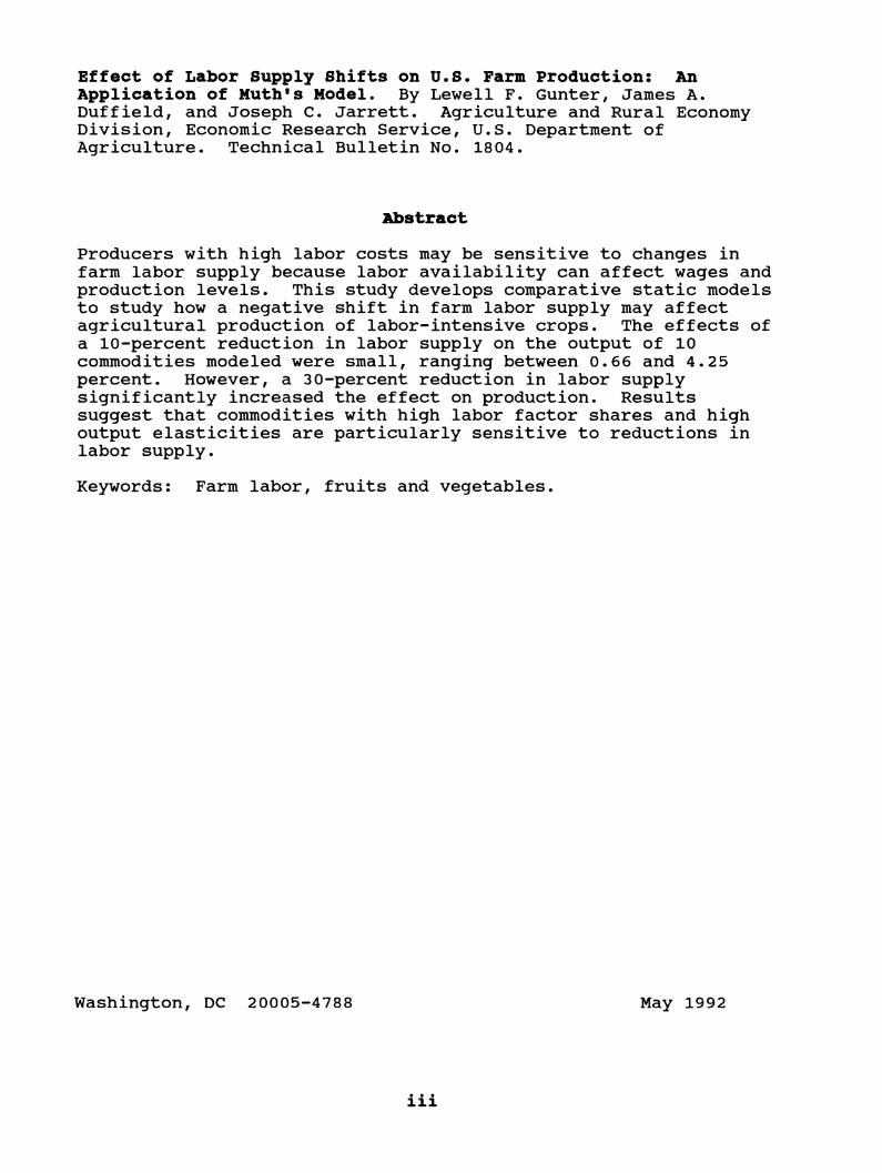
Effect of Labor Supply Shifts on U.S. Farm Production: An Application of Muth*s Model. By Lewell F. Gunter, James A. Duffield, and Joseph C. Jarrett. Agriculture and Rural Economy Division, Economic Research Service, U.S. Department of Agriculture. Technical Bulletin No. 1804.

3a>stract

Producers with high labor costs may be sensitive to changes in farm labor supply because labor availability can affect wages and production levels. This study develops comparative static models to study how a negative shift in farm labor supply may affect agricultural production of labor-intensive crops. The effects of a 10-percent reduction in labor supply on the output of 10 commodities modeled were small, ranging between 0.66 and 4.25 percent. However, a 30-percent reduction in labor supply significantly increased the effect on production. Results suggest that commodities with high labor factor shares and high output elasticities are particularly sensitive to reductions in labor supply.

Keywords: Farm labor, fruits and vegetables.

Washington, DC 20005-4788 May 1992

• • • 111

Contents

Page

i;ntroduction 1

Theoretical Framework 2

Model Implementation 4

Empirical Analysis 5 Revenue Factor Shares 5 Input Supply Elasticities 5 Elasticity of Substitution and Technological Shifts 6 Output Demand Elasticities and Demand Shifts 7

Results 9 Results from the 5-Year Aggregate Model 10 Results from Commodity Models 11 Results for a 30-Percent Decrease in Labor Supply 16

Summary and Conclusions 16

References 18

IV

Effect of Labor Supply Shifts on U.S. Farm Production

An Application of Muth's Model

Lewell F. Gunter James A. Duffield Joseph C. Jarrett

Introduction

A methodology is developed in this report to help evaluate the effects of labor supply shifts on the farm labor market and agricultural production. We used comparative static analysis to show how reductions in labor supply will affect production of 10 selected fresh market fruit and vegetable crops. This paper focuses on the effects of a labor supply reduction, but the methodology can be used to analyze the effect of a positive labor supply shift or other shocks to equilibrium conditions in the U.S. farm labor market.

Mechanization has significantly reduced labor requirements for most field crop and livestock producers. Labor, nonetheless, continues to be a critical input in the production of many fruits and vegetables. Hired labor's share of total cash operating expenses averages about 37 percent on U.S. vegetable farms and about 40 percent on fruit farms (Oliveira). In contrast, labor expenses on cash grain and dairy farms are only about 10 percent of total farm production expenses.

Producers with high labor costs may be sensitive to changes in farm labor supply because labor availability can affect wages and production levels. However, to estimate the full effects of a labor supply shift on producton, labor's relationship with other input and output variables must be considered. The purpose of this study is to develop a method that incorporates these variables into a model to analyze the effects of labor supply shifts on agricultural production.

Lewell F. Gunter is an associate professor in the Department of Agricultural Economics, University of Georgia; James A. Duffield is an economist in the Agriculture and Rural Economy Division, Economic Research Service; Joseph C. Jarrett is a former graduate assistant in the Department of Agricultural Economics, University of Georgia.

Theoretical Freuneworlc

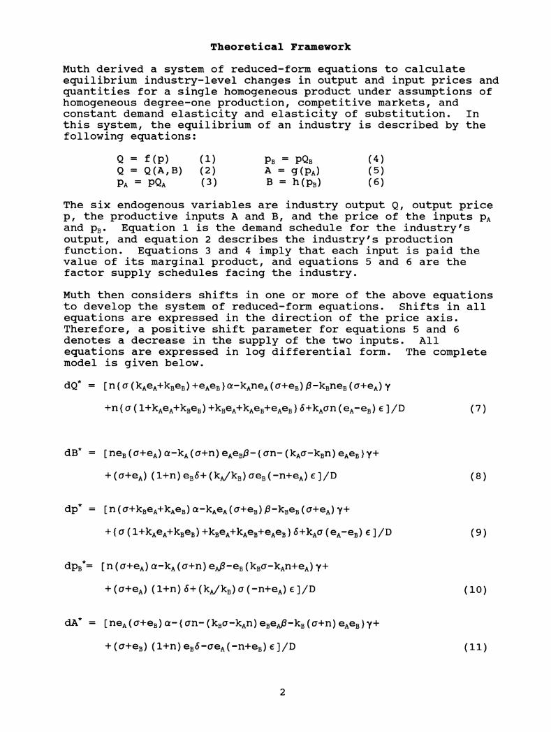
Muth derived a system of reduced-form equations to calculate equilibrium industry-level changes in output and input prices and quantities for a single homogeneous product under assumptions of homogeneous degree-one production, competitive markets, and constant demand elasticity and elasticity of substitution. In this system, the equilibrium of an industry is described by the following equations:

Q = f(P) (1) PB = PQB (4) Q = Q(A,B) (2) A = g (PA) (5) PA = PQA (3) B = h(PB) (6)

The six endogenous variables are industry output Q, output price p, the productive inputs A and B, and the price of the inputs p^ and Pß. Equation 1 is the demand schedule for the industry's output, and equation 2 describes the industry's production function. Equations 3 and 4 imply that each input is paid the value of its marginal product, and equations 5 and 6 are the factor supply schedules facing the industry.

Muth then considers shifts in one or more of the above equations to develop the system of reduced-form equations. Shifts in all equations are expressed in the direction of the price axis. Therefore, a positive shift parameter for equations 5 and 6 denotes a decrease in the supply of the two inputs. All equations are expressed in log differential form. The complete model is given below.

dQ* = [n{a(kAeA+kBeB)+eAeB}a-kAneA(a+eB))8-kBneB(a+eA)Y

+n{a (l+k^eA+kBeB) +kBeA+kAeB4-eAeB}Ä+k^an(e^-eB) e ]/D (7)

dB* = [neB(a+eA)a-kA(a+n)eAeBi3-{an-(kAa-kBn)eAeB}Y+

+ (a+eA) (l+n)eB5+(kA/kB)aeB(-n+eA)€]/D (8)

dp* = [n(a+kBeA4-kAeB)a-kAeA(a+eB))S-kBeB(a+eA)Y+

+ {a (l+k^e^+kBeB) +kBeA+kAeB+eAeB} i+k^a (e^-e^) e]/D (9)

dPB*= [n (a+e^) a-k^(a+n) eJ3-e^ (kBa-k^n+eA) Y+

+ (a+eA) (l+n)(S+(kA/kB)a(-n+eJe]/D (10)

dA* = [neA(a+eB)a-{an-(kBa-kAn)eBeA)8-kB(a+n)eAeB}Y+

+ (a+eB) (H-n)eB(S-aeA(-n+eB)e]/D (11)

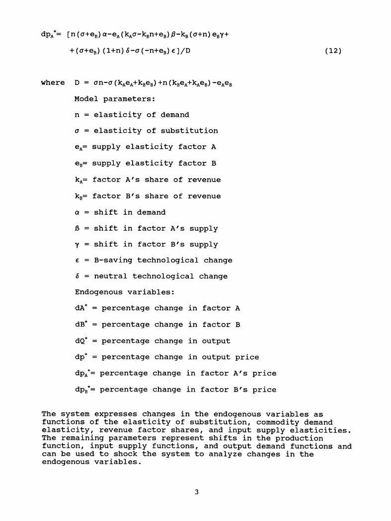
dp/= [n (a+Gß) a-e^(kACJ-ken+eB) jS-kß (a+n) eBY+

+ (a+eB) (l+n)5-a(-n+eB)€]/D (12)

where D = an-a(kAeA+kBeB)+n(kBeA+kAeB)-e^eB

Model parameters:

n = elasticity of demand

o = elasticity of substitution

ep= supply elasticity factor A

eB= supply elasticity factor B

kA= factor A^s share of revenue

kB= factor B's share of revenue

a = shift in demand

ß = shift in factor A^s supply

Y = shift in factor B's supply

e = B-saving technological change

<S = neutral technological change

Endogenous variables:

dA* = percentage change in factor A

dB* = percentage change in factor B

dQ* = percentage change in output

dp* = percentage change in output price

dPA*= percentage change in factor A^s price

dPB*= percentage change in factor B's price

The system expresses changes in the endogenous variables as functions of the elasticity of substitution, commodity demand elasticity, revenue factor shares, and input supply elasticities. The remaining parameters represent shifts in the production function, input supply functions, and output demand functions and can be used to shock the system to analyze changes in the endogenous variables.

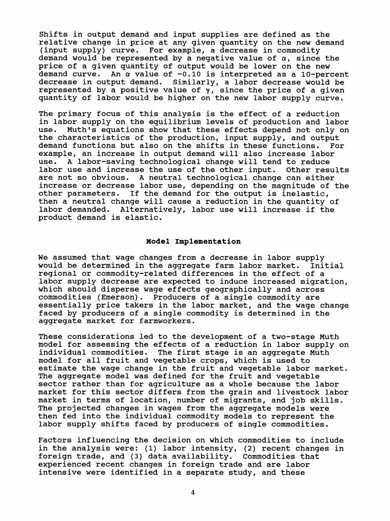
Shifts in output demand and input supplies are defined as the relative change in price at any given quantity on the new demand (input supply) curve. For example, a decrease in commodity demand would be represented by a negative value of a, since the price of a given quantity of output would be lower on the new demand curve. An a value of -0.10 is interpreted as a 10-percent decrease in output demand. Similarly, a labor decrease would be represented by a positive value of y, since the price of a given quantity of labor would be higher on the new labor supply curve.

The primary focus of this analysis is the effect of a reduction in labor supply on the equilibrium levels of production and labor use. Muth's equations show that these effects depend not only on the characteristics of the production, input supply, and output demand functions but also on the shifts in these functions. For example, an increase in output demand will also increase labor use. A labor-saving technological change will tend to reduce labor use and increase the use of the other input. Other results are not so obvious. A neutral technological change can either increase or decrease labor use, depending on the magnitude of the other parameters. If the demand for the output is inelastic, then a neutral change will cause a reduction in the quantity of labor demanded. Alternatively, labor use will increase if the product demand is elastic.

Model Implementation

We assumed that wage changes from a decrease in labor supply would be determined in the aggregate farm labor market. Initial regional or commodity-related differences in the effect of a labor supply decrease are expected to induce increased migration, which should disperse wage effects geographically and across commodities (Emerson). Producers of a single commodity are essentially price takers in the labor market, and the wage change faced by producers of a single commodity is determined in the aggregate market for farmworkers.

These considerations led to the development of a two-stage Muth model for assessing the effects of a reduction in labor supply on individual commodities. The first stage is an aggregate Muth model for all fruit and vegetable crops, which is used to estimate the wage change in the fruit and vegetable labor market. The aggregate model was defined for the fruit and vegetable sector rather than for agriculture as a whole because the labor market for this sector differs from the grain and livestock labor market in terms of location, number of migrants, and job skills. The projected changes in wages from the aggregate models were then fed into the individual commodity models to represent the labor supply shifts faced by producers of single commodities.

Factors influencing the decision on which commodities to include in the analysis were: (1) labor intensity, (2) recent changes in foreign trade, and (3) data availability. Commodities that experienced recent changes in foreign trade and are labor intensive were identified in a separate study, and these

commodities were chosen whenever data were available (Duffield and Gunter). Data availability, however, dictated that only fresh fruits and vegetables could be used in this analysis. In total, 10 commodities were analyzed in the empirical model: tomatoes, broccoli, cauliflower, sweetpotatoes, carrots, grapes, oranges, grapefruit, peaches, and apples.

Empirical Analysis

Equations 7-12 were solved for a 5-year time horizon to allow markets to adjust to the labor shift. The 5-year horizon was implemented through the use of long-term elasticities and the conversion of annual demand shifts to 5-year shifts. Detailed results are reported for a 10-percent decline in farm labor supply, and an overview of results is presented for a 30-percent decline in labor supply.

The following parameter estimates were needed in both the aggregate and commodity-specific models. Estimates for these parameters were obtained from previous research or directly estimated.

Revenue Factor Shares

Aggregate labor expense as a percentage of total revenue is about 29 percent for the production of fruits and vegetables (1987 Census of Agriculture). Since the inputs are classified as labor and nonlabor, 71 percent was used as the nonlabor factor share in the aggregate model. Factor shares for the individual commodity models were determined from commodity budgets obtained from Cooperative Extension Service offices in major fruit- and vegetable-producing States.

Input Supply Elasticities

An aggregate farm labor supply elasticity for the United States was available in the literature, but a labor supply elasticity for the production of fruits and vegetables was not. Longrun labor supply elasticity estimates range between 0.71 and 1.55 (Duffield). These values were used as benchmarks in the first- stage model. Since fruit and vegetable production employs only a portion of the total U.S. agricultural workforce, the labor supply for this single sector should be more elastic than the aggregate U.S. farm labor supply. The high estimate of the labor elasticity was thus chosen as the baseline value. Nonlabor inputs were assumed to be perfectly elastic in supply.

From the national labor market perspective, changes in production of any individual fruit and vegetable can be assumed to have little effect on wage rates, and the labor supply elasticity to each industry should be very elastic. Although specific labor supply elasticity values for the fruit and vegetables included in this report could not be determined, the sensitivity of the empirical model was tested for labor supply elasticities ranging from 7 to 15. Results of the sensitivity analysis indicate that

the model is not very sensitive to labor supply elasticity, and a labor supply elasticity of 10 was used in the individual commodity models. This value implies that a 10-percent decline in labor use for an individual commodity would be associated with a 1-percent decline in the wage rate. The supply of nonlabor inputs was assumed to be perfectly elastic in the commodity models.

Elasticity of Substitution and Technological Shifts

A wide range of aggregate elasticities of substitution is available from past studies (Gunter and Vasavada, Brown and Christensen, and Ray). Gunter and Vasavada estimated the elasticity of substitution between seasonal agricultural labor and capital to be 0.63 in the short run and 2.11 in the long run. The elasticity of substitution estimated by Brown and Christensen between all hired labor and capital was 0.32 in the short run, while Ray's estimate of the longrun elasticity of substitution between hired labor and capital was 0.75. The elasticity of substitution needed for the empirical model should reflect the substitutability of hired labor and nonlabor inputs for fruit and vegetable production. Since this estimate is not available in the literature, the Muth equations were solved using the extreme values of the longrun estimates of general agriculture, which ranged between 0.75 and 2.11. The low value was considered the baseline for the aggregate model, since fruit and vegetable production is more labor intensive than other sectors of agriculture, and mechanical harvesting technology is unavailable for many fresh market fruits and vegetables.

The Muth equations permit inclusion of parameters that represent Hicks-neutral and labor-saving technological change. Estimates of technological progress in fruit and vegetable production were unavailable. Estimates of technological progress rates for aggregate U.S. agriculture range from technological regression to a 1.8-percent annual increase (Capalbo and Vo, p. 119). Given the unavailability of specific technology estimates for fruits and vegetables, the variations in the estimates of technological progress for general U.S. agriculture and the relatively short 5-year time horizon of the model, no technological change was assumed for the first-stage Muth simulations.

In the individual commodity models, elasticity of substitution estimates from the first-stage model were used, and technological progress was assumed to be zero. Conceptually, the elasticity of substitution is likely to be different for each commodity. The elasticity of substitution should reflect the state of present technology. Brown summarized the state of production technology of numerous fruits and vegetables. Partially mechanized commodities should have a higher elasticity of substitution than hand-harvested commodities or commodities that are entirely harvested by machine, because the present technology may be adaptable to more acreage with an increase in the wage rate. For the fresh market commodities considered here, only tomatoes and apples are partially mechanically harvested, and the high elasticity of substitution value, 2.11, was used as the baseline

for these crops. The other crops in this report are hand harvested, so the low value of 0.75 was used as the baseline for those crops.

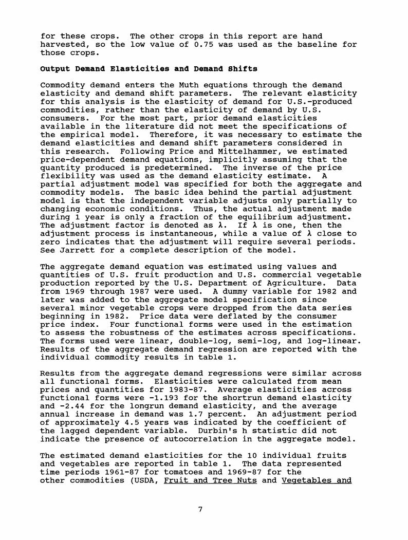
Output Demand Elasticities and Demand Shifts

Commodity demand enters the Muth equations through the demand elasticity and demand shift parameters. The relevant elasticity for this analysis is the elasticity of demand for U.S.-produced commodities, rather than the elasticity of demand by U.S. consumers. For the most part, prior demand elasticities available in the literature did not meet the specifications of the empirical model. Therefore, it was necessary to estimate the demand elasticities and demand shift parameters considered in this research. Following Price and Mittelhammer, we estimated price-dependent demand equations, implicitly assuming that the quantity produced is predetermined. The inverse of the price flexibility was used as the demand elasticity estimate. A partial adjustment model was specified for both the aggregate and commodity models. The basic idea behind the partial adjustment model is that the independent variable adjusts only partially to changing economic conditions. Thus, the actual adjustment made during 1 year is only a fraction of the equilibrium adjustment. The adjustment factor is denoted as A. If A. is one, then the adjustment process is instantaneous, while a value of X close to zero indicates that the adjustment will require several periods. See Jarrett for a complete description of the model.

The aggregate demand equation was estimated using values and quantities of U.S. fruit production and U.S. commercial vegetable production reported by the U.S. Department of Agriculture. Data from 1969 through 1987 were used. A dummy variable for 1982 and later was added to the aggregate model specification since several minor vegetable crops were dropped from the data series beginning in 1982. Price data were deflated by the consumer price index. Four functional forms were used in the estimation to assess the robustness of the estimates across specifications. The forms used were linear, double-log, semi-log, and log-linear. Results of the aggregate demand regression are reported with the individual commodity results in table 1.

Results from the aggregate demand regressions were similar across all functional forms. Elasticities were calculated from mean prices and quantities for 1983-87. Average elasticities across functional forms were -1.193 for the shortrun demand elasticity and -2.44 for the longrun demand elasticity, and the average annual increase in demand was 1.7 percent. An adjustment period of approximately 4.5 years was indicated by the coefficient of the lagged dependent variable. Durbin's h statistic did not indicate the presence of autocorrelation in the aggregate model.

The estimated demand elasticities for the 10 individual fruits and vegetables are reported in table 1. The data represented time periods 1961-87 for tomatoes and 1969-87 for the other commodities (USDA, Fruit and Tree Nuts and Vegetables and

Table 1--Summary statistics from demand regressions

Commodity Shortrun elasticity^

Longrun elasticity

Annual demand shift

Adjustment coefficient

00

Aggregate fruits and vegetables

Apples

Broccoli

Carrots

Cauliflower

Grapefruit

Grapes

Oranges

Peaches

Sweet- potatoes

Tomatoes

Range Mean Range Mean Range Mean Mean Mean

■1.096 •1.295

-1.193 -2.30 -2.60

-2.44 0.016 .018

0.017 0.512 0.789

-.465 -.581

-.518 -1.03 -1.17

-1.09 .016 .023

.019 .527 .818

0 ■1.629

-.733 0 -1.63

-.73 NA 0 .363 .967

-.863 ■1.340

-1.083 -.86 -1.34

-1.08 NA 0 0^ .685

1.329 2.469

-1.812 -1.33 -6.08

-3.21 .020 .038

.027 .276 .932

-.806 -.846

-.826 -1.169 -1.76

-1.74 NA 0 .54 .627

-.676 -.917

-.792 -1.14 -1.64

-1.38 0 .006 .423 .592

-.414 -.455

-.434 -.41 -.46

-.43 .028 .028

.028 0^ .752

1.946 2.388

-2.164 -3.27 -3.54 -.019 -.022

-.021 .390 .854

-.380 -.433

-.407 -1.09 1.14

-1.12 NA 0 .638 .727

-.958 1.388

-1.157 -1.86 -2.62

-2.21 0 .009

.004 .477 .848

NA = Not applicable. ^ Values in table reflect results of estimation for four functional forms: linear, log-linear, semi-log, and double-log for all commodities. ^ Demand elasticities were close to those reported by Price and Mittelhammer for the four commodities for which comparisons were available. They used 1949-73 data and derived estimates for apples (-0.596), grapefruit (-0.675), grapes (-1.168), oranges (-0.660), and peaches (-2.76). Coefficients not significantly different from zero for any functional form.

Specialties).^ The same functional forms used in the aggregated demand model were also used to estimate the individual commodity demands. Differences in estimated longrun demand elasticities across functional forms were less than 1 for all commodities except broccoli and cauliflower. Durbin's h statistic did not indicate the presence of autocorrelation in any of the equations. Average shortrun elasticities across functional forms ranged from lows of -0.434 and -0.407 for oranges and sweetpotatoes, respectively, to highs of -1.82 and -2.16 for cauliflower and peaches, respectively. Broccoli and oranges, the commodities with the lowest longrun demand elasticities, had mean values of -0.73 and -0.43, respectively. As with the shortrun case, cauliflower and peaches had the highest longrun demand elasticities with mean values of -3.21 and -3.54, respectively. The slowest adjustment to equilibrium was found for sweetpotatoes, which had an average (1-A.) value of 0.638. The results for carrots and oranges indicated immediate adjustment, since the estimates of (1-X) for these commodities were not significant.

The demand shifts, such as those associated with changes in income or taste and preference, were collapsed into a single demand-shift term, which is consistent with the requirements of the Muth model. These demand shifts were captured in the time trend from the estimated model, and were readily usable since the Muth model expresses demand shifts in price space and the estimated demand equations were price dependent. The results indicated no shifts in demand for broccoli, carrots, grapefruit, and sweetpotatoes, due to the insignificant time trend coefficients. Demand for apples, cauliflower, grapes, oranges, and tomatoes increased moderately. Demand for peaches decreased. The mean values of the elasticities and demand shift parameters from the four functional forms were used in the Muth equations for all commodities except broccoli and cauliflower. The average values from the linear and log-linear forms were used for these two commodities. From 1969 to 1987, broccoli and cauliflower had the largest variations in output of all fruits and vegetables considered in this report. The ratio of the largest to the smallest annual output during this period was 9.28 for broccoli, 4.65 for cauliflower, and 2.79 for the next highest crop, carrots. This contributes to the differences in the broccoli and cauliflower results for the functional forms, using log quantity versus those using quantity, and supports the use of the linear and log-linear specifications for these crops.

Results

Due to limited information about specific parameters in the literature, we tested the sensitivity of the model to selected

Results from the demand estimation for tomatoes, using 1969-87 data, suggested multicollinearity problems, with high goodness-of-fit measures but low significance for the coefficients. Consistent data for tomatoes were available back to 1961, and those data were included to reduce the multicollinearity problem.

parameters. We performed a sensitivity analysis on the elasticity of substitution, labor supply elasticity, labor shift parameter, and technology parameters. A 5-year horizon with a 10-percent shift in the aggregate labor supply was used in the sensitivity analysis. A complete description of this procedure is provided by Jarrett.

The elasticity of substitution was parameterized from zero to 2.11, which represented the highest value found in the literature. It appeared to have little effect on output and more of an effect on labor use for the range of values tested. The labor supply elasticity in the commodity models, which was parameterized between 7 and 15, had no significant effect on commodities with relatively low shortrun demand elasticities. For commodities with extremely elastic demands, however, the labor supply elasticity does have some effect on output. The two technology parameters have different effects on the results of the model. The parameter reflecting neutral technological change has an important effect on both output and labor use. A wide range of solutions was observed, with the effect on production and labor use becoming more pronounced with higher elasticities of demand. Labor-saving technology, on the other hand, had little effect on the model results. The sensitivity of output to changes in the labor shift parameter can be approximated by a near linear relationship. For example, when shifting labor between a 5- and 15-percent range, a 5-percent change will reduce output by approximately half as much as a 10-percent change in labor supply.

Results from the 5-Year Aggregate Model

The first-stage Muth equations with a 5-year time horizon were solved for aggregate fruits and vegetables for labor supply shifts of zero and 10 percent. Given the uncertainty about the value of several parameters, two values, 0.75 and 2.11, were used for the elasticity of substitution, and the labor supply elasticity was parameterized at 0.710 and 1.55. Values for demand elasticity and the 5-year demand shift were -2.44 and 0.088, respectively. Labor's factor share was 0.29, nonlabor supply elasticity was 9,999 (indicating perfect elasticity), and the technology shift equaled zero. Results are given in table 2.

Output is projected to increase even with a decline in labor supply because increases in output demand outweigh the labor supply effect. Increasing the elasticity of substitution increases the projected growth in output and reduces the growth in labor use and wages. A higher labor supply elasticity generally increases the growth in output and labor use but reduces the increase in wage rates.

Figure 1 shows the equilibrium wage shift from a 10-percent decline in labor supply for a range of values of the elasticity of substitution and labor supply elasticity. The effects of these elasticities on wages are strong when both parameters are below 0.5. When either elasticity is greater than 0.5, however.

10

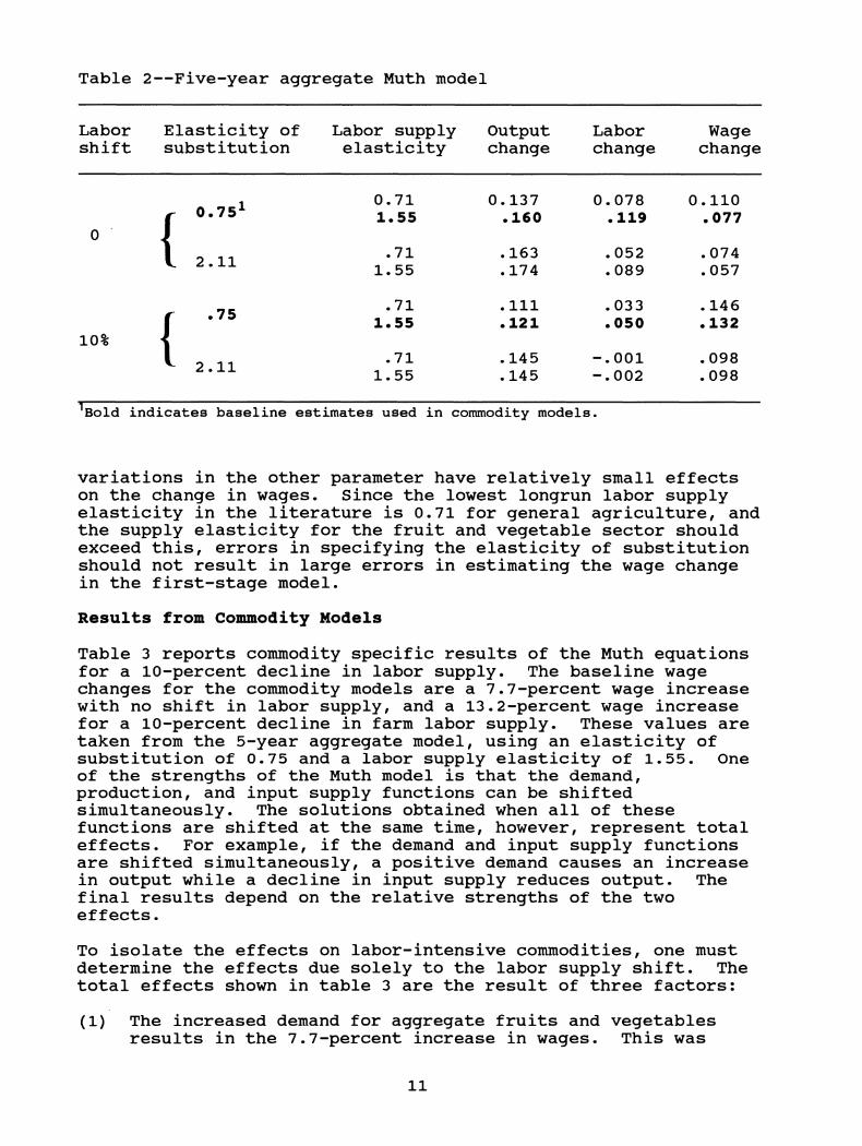
Table 2—Five-year aggregate Muth model

Labor Elasticity of Labor supply Output Labor Wage shift substitution elasticity change change change

{ 0.75^

2.11

10% { " *- 2.11

0.71 0.137 0.078 0.110 1.55 .160 .119 .077

.71 .163 .052 .074 1.55 .174 .089 .057

.71 .111 .033 .146 1.55 .121 .050 .132

.71 .145 -.001 .098 1.55 .145 -.002 .098

T Bold indicates baseline estimates used in commodity models.

variations in the other parameter have relatively small effects on the change in wages. Since the lowest longrun labor supply elasticity in the literature is 0.71 for general agriculture, and the supply elasticity for the fruit and vegetable sector should exceed this, errors in specifying the elasticity of substitution should not result in large errors in estimating the wage change in the first-stage model.

Results from Commodity Models

Table 3 reports commodity specific results of the Muth equations for a 10-percent decline in labor supply. The baseline wage changes for the commodity models are a 7.7-percent wage increase with no shift in labor supply, and a 13.2-percent wage increase for a 10-percent decline in farm labor supply. These values are taken from the 5-year aggregate model, using an elasticity of substitution of 0.75 and a labor supply elasticity of 1.55. One of the strengths of the Muth model is that the demand, production, and input supply functions can be shifted simultaneously. The solutions obtained when all of these functions are shifted at the same time, however, represent total effects. For example, if the demand and input supply functions are shifted simultaneously, a positive demand causes an increase in output while a decline in input supply reduces output. The final results depend on the relative strengths of the two effects.

To isolate the effects on labor-intensive commodities, one must determine the effects due solely to the labor supply shift. The total effects shown in table 3 are the result of three factors:

(1) The increased demand for aggregate fruits and vegetables results in the 7.7-percent increase in wages. This was

11

Figure 1

Effect of elasticity of substitution and labor supply elasticity on the equilibrium wage change^

<7:^n> ^\.^^'

-^ Sul>^*''''

\abor supply shift, -10.0 percent; output demand shift, 8.8 percent; demand elasticity, -2.44; labor share, 0.29; technology shift, zero. Drop lines for elasticity of substitution, 0.75 and 2.0; labor supply elasticity, 0.75 and 1.5.

12

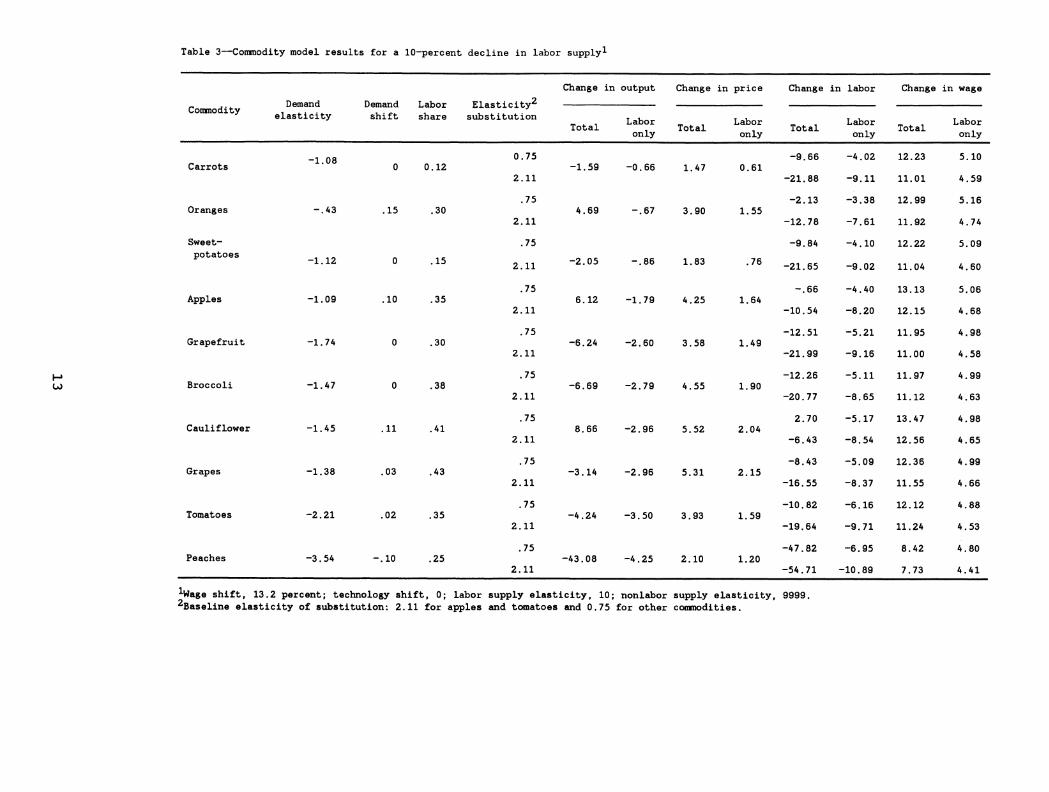
Table 3—Commodity model results for a 10-percent decline in labor supply^

Change in output Change in price Change in Isüsor Change in wage

Commodity Demand Demand Labor Elasticity^

elasticity shift share substitution

LJ

Carrots

Oranges

Sweet- potatoes

Apples

Grapefruit

Broccoli

Cauliflower

Grapes

Tomatoes

Peaches

_ ^ , Labor „ ^ , Labor Total , Total

only only

-1.08

-.43

-1.12

-1.09

-1.74

-1.47

-1.45

-1.38

-2.21

-3.54

0 0.12

.15 .30

0 .15

.10 .35

0 .30

0 .38

.11 .41

.03 .43

.02 .35

-.10 .25

0.75

2.11

.75

2.11

.75

2.11

.75

2.11

.75

2.11

.75

2.11

.75

2.11

.75

2.11

.75

2.11

.75

2.11

-1.59 -0.66 1.47 0.61

4.69 -.67 3.90 1.55

-2.05 -.86 1.83 .76

6.12 -1.79 4.25 1.64

-6.24 -2.60 3.58 1.49

-6.69 -2.79 4.55 1.90

8.66 -2.96 5.52 2.04

-3.14 -2.96 5.31 2.15

-4.24 -3.50 3.93 1.59

-43.08 -4.25 2.10 1.20

Total Labor only

Total Labor only

-9.66 -4.02 12.23 5.10

-21.88 -9.11 11.01 4.59

-2.13 -3.38 12.99 5.16

-12.78 -7.61 11.92 4.74

-9.84 -4.10 12.22 5.09

-21.65 -9.02 11.04 4.60

-.66 -4.40 13.13 5.06

-10.54 -8.20 12.15 4.68

-12.51 -5.21 11.95 4.98

-21.99 -9.16 11.00 4.58

-12.26 -5.11 11.97 4.99

-20.77 -8.65 11.12 4.63

2.70 -5.17 13.47 4.98

-6.43 -8.54 12.56 4.65

-8.43 -5.09 12.36 4.99

-16.55 -8.37 11.55 4.66

-10.82 -6.16 12.12 4.88

-19.64 -9.71 11.24 4.53

-47.82 -6.95 8.42 4.80

-54.71 -10.89 7.73 4.41

^Wage shift, 13.2 percent; technology shift, 0; labor supply elasticity, 10; nonlíÚDor supply elasticity, ^Baseline elasticity of substitution; 2.11 for apples amd tomatoes and 0.75 for other commodities.

9999.

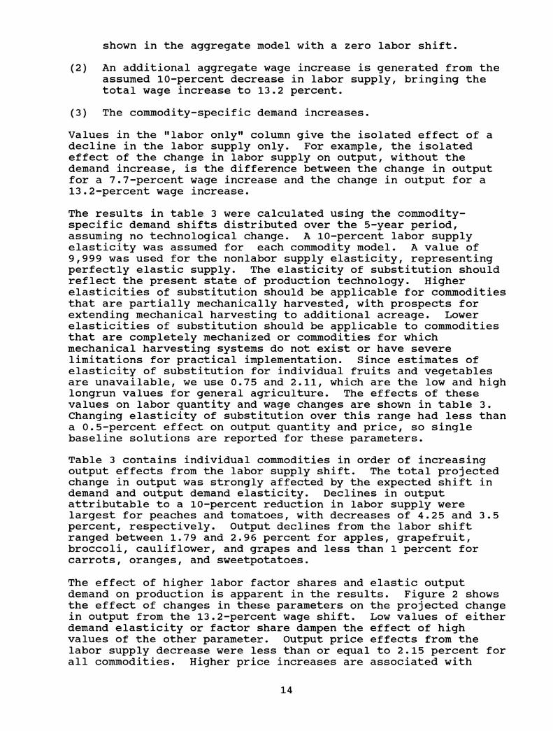
shown in the aggregate model with a zero labor shift.

(2) An additional aggregate wage increase is generated from the assumed 10-percent decrease in labor supply, bringing the total wage increase to 13.2 percent.

(3) The commodity-specific demand increases.

Values in the "labor only" column give the isolated effect of a decline in the labor supply only. For example, the isolated effect of the change in labor supply on output, without the demand increase, is the difference between the change in output for a 7.7-percent wage increase and the change in output for a 13.2-percent wage increase.

The results in table 3 were calculated using the commodity- specific demand shifts distributed over the 5-year period, assuming no technological change. A 10-percent labor supply elasticity was assumed for each commodity model. A value of 9,999 was used for the nonlabor supply elasticity, representing perfectly elastic supply. The elasticity of substitution should reflect the present state of production technology. Higher elasticities of substitution should be applicable for commodities that are partially mechanically harvested, with prospects for extending mechanical harvesting to additional acreage. Lower elasticities of substitution should be applicable to commodities that are completely mechanized or commodities for which mechanical harvesting systems do not exist or have severe limitations for practical implementation. Since estimates of elasticity of substitution for individual fruits and vegetables are unavailable, we use 0.75 and 2.11, which are the low and high longrun values for general agriculture. The effects of these values on labor quantity and wage changes are shown in table 3. Changing elasticity of substitution over this range had less than a 0.5-percent effect on output quantity and price, so single baseline solutions are reported for these parameters.

Table 3 contains individual commodities in order of increasing output effects from the labor supply shift. The total projected change in output was strongly affected by the expected shift in demand and output demand elasticity. Declines in output attributable to a 10-percent reduction in labor supply were largest for peaches and tomatoes, with decreases of 4.25 and 3.5 percent, respectively. Output declines from the labor shift ranged between 1.79 and 2.96 percent for apples, grapefruit, broccoli, cauliflower, and grapes and less than 1 percent for carrots, oranges, and sweetpotatoes.

The effect of higher labor factor shares and elastic output demand on production is apparent in the results. Figure 2 shows the effect of changes in these parameters on the projected change in output from the 13.2-percent wage shift. Low values of either demand elasticity or factor share dampen the effect of high values of the other parameter. Output price effects from the labor supply decrease were less than or equal to 2.15 percent for all commodities. Higher price increases are associated with

14

Figure 2

Effect of demand elasticity and labor share on the change in output from a 10- percent decrease in labor supply^

^^e>^o^

^Elasticity of substitution, 0.75; labor supply elasticity, 10; wage increase, 13.2 percent; no demand shift; and nonlabor factor has perfectly elastic supply.

15

higher labor factor shares and less elastic output demand.

Changes in labor use resulting from the labor supply shift paralleled changes in output induced by the shift. Higher demand elasticities and higher labor shares were associated with greater reductions in labor use. When we raised the elasticity of substitution from 0.75 to 2.11 percent, labor use declined by as much as 5.5 percent. The effect of elasticity of substitution on labor use was greatest for commodities with the smallest baseline changes in labor use.

Projected wage changes are associated with changes in output and labor use and are, therefore, dependent on the parameters affecting these changes. In general, the total wage changes were near the wage shift value of 13.2 percent when projected changes in labor use were small and were lower (greater) than the shift values when labor use declined (rose).

Results for a 30-Percent Decrease in Labor Supply

The aggregate and commodity Muth equations were also solved for a 30-percent decline in labor supply. With this strong shift, the baseline aggregate wage rose by 24.4 percent. The relative effects on crop production were the same as for a 10-percent decline in labor. The decreases in output attributable to the 30-percent decline in labor supply were 12.9 percent for peaches and 10.6 percent for tomatoes. Output declines for apples, grapefruit, broccoli, cauliflower, and grapes ranged between 5.42 percent (apples) and 8.99 percent (grapes and cauliflower). Output declines for carrots, oranges, and sweetpotatoes were less than 3 percent.

Summary and Conclusions

The effect of a 10-percent reduction in labor supply on the output of the 10 commodities considered here, was less than 5 percent. A 3 0-percent reduction in labor supply increased the effect considerably. Output demand elasticity and labor factor share appeared to be the most important factors influencing the effect of labor supply shifts on production. For example, among the commodities analyzed, peaches and tomatoes showed the highest reduction in output. They also had the largest demand elasticities and both commodities had moderately high labor shares. These results demonstrate the importance of output price and competition on the production of labor-intensive crops. Producers of tomatoes and peaches in the United States have to compete with a strong import market. Mexican growers are very active in the U.S. winter tomato market, and processed peaches from Mediterranean countries and other fruits provide competition for U.S. fresh peaches if peach prices rise too high. On the other hand, producers who face little foreign competition or are protected by high import tariffs may be more inclined to raise output price to offset higher labor costs.

A potentially significant limitation of the fruit and vegetable

16

projections relates to the use of an aggregate U.S. model for the calculations. Regional differences in demand elasticities and labor supply conditions could contribute to significant local differences in output effects. Regional differences in demand elasticities are related to both the extent of the market and the timing of harvest. Higher-than-average demand elasticities are likely for producers from regions that market their commodities during periods with substantial competition from other regions. Residual suppliers and producers from regions attempting to penetrate markets also would be expected to face more elastic demand for their output. Given the strong effect of the demand elasticity, these producers are more vulnerable to the effects of a given shift in labor supply.

Regional differences in labor supply could be reflected either through differences in the labor supply shift or differences in regional labor supply elasticities. Producers facing less elastic labor supplies will be shielded to some extent from a labor supply shift, since wages may drop more as labor use declines.

The Muth framework is easily adaptable to modeling regional differences in the effects of labor supply shifts if appropriate regional parameter values can be determined. Estimates of regional parameters are scarce, however, so new sources of information are needed to conduct regional level research.

17

References

Brown, G.K. "Fruit and Vegetable Mechanization," Migrant Labor in Agriculture—An International Comparison, Philip L. Martin (ed.)- University of California, Giannini Foundation of Agricultural Economics and the German Marshall Fund of the United States, (1985):195-210,

Brown, R.S., and L.R. Christensen. "Estimating Elasticities of Substitution in a Model of Partial Static Equilibrium: An Application to U.S. Agriculture, 1947-74," Modeling and Measuring Natural Resource Substitution. E. Berndt and B. Field (eds.). Cambridge, MA: MIT Press, 1981.

Capalbo, S.M., and T.T. Vo. "A Review of the Evidence on Agricultural Productivity and Aggregate Technology," Agricultural Productivity; Measurement and Explanation. Susan M. Capalbo and John A. Antle (eds.). Washington, DC: Resources for the Future, 1988.

Duffield, James A. Estimating Farm Labor Elasticities to Analyze the Effects of Immigration Reform. Staff Report AGES-9013, U.S. Dept. Agr., Econ. Res. Serv., Feb. 1990.

Duffield, James A., and Lewell Gunter. Will Immigration Reform Affect the Economic Competitiveness of Labor-Intensive Crops? Staff Report AGES-9126, U.S. Dept. Agr., Econ. Res. Serv., May 1991.

Emerson, Robert D. "Migratory Labor and Agriculture," American Journal of Agricultural Economics. 71(1989):617-29.

Gunter, Lewell, and Utpal Vasavada. "Dynamic Labor Demand Schedules for U.S. Agriculture," Applied Economics, 20(1988):803- 13.

Jarrett, Joseph C. "Impacts of Immigration Reform on Labor- intensive Agriculture." Unpublished M.S. thesis. University of Georgia, Athens, 1990.

Muth, R.F. "The Derived Demand Curve for a Productive Factor and the Industry Supply Curve," Oxford Economics Papers, 16(1964):221-34.

Oliveira, Victor J. Hired and Contract Labor in U.S. Agriculture, 1987: A Regional Assessment of Structure. AER-648, U.S. Dept. Agr., Econ. Res. Serv., May 1991.

Price, D.W., and R.C. Mittelhammer. "A Matrix of Demand Elasticities for Fresh Fruit," Western Journal of Agricultural Economics, 4(1979): 69-86.

Ray, S.C. "A Translog Cost Function Analysis of U.S. Agriculture, 1939-1977," American Journal of Agricultural Economics. 64(1982):490-98.

18

NATIONAL AGRICULTURAL LIBRARY

1022458052 U.S. Department of Agriculture, Economie Research Service. rruxu and Tree Nuts Situation and Outlook Yearbook. TFS-250, 1989 and earlier issues.

U.S. Department of Agriculture, Economie Research Service. Vegetables and Specialties Situation and Outlook Yearbook. TVS- 249, 1989 and earlier issues.

U.S. Department of Commerce, Bureau of the Census. 1987 Census of Agriculture. Volume 1, Geographic Area Series, Part 51. United States Summary and State Data. 1989.

19