Chen Cai, Benjamin Heydecker

Presentation for the 4th CREST Open Workshop

Operation Research for Software Engineering Methods, London, 2010

Approximate Dynamic Programming Approximate Dynamic Programming & Adaptive Traffic Control& Adaptive Traffic Control

Contents

• Dynamic Programming• Curse of Dimensionality• Approximate Dynamic Programming• Adaptive Traffic Signal Control

1. Dynamic Programming

1. Dynamic Programming

• What it does?– Sequential decision-making for discrete systems– Iterative computing rather than enumeration– Global optimality

t0 t1 t2 t3 tm-2 tmtm-1

Stage 0 Stage m-1

t

F = i0,u0

∗,w0 , i1 ,u1∗,w1 ,..., im−1 ,um−1

∗ ,wm−1 , im{ }

1. Dynamic Programming

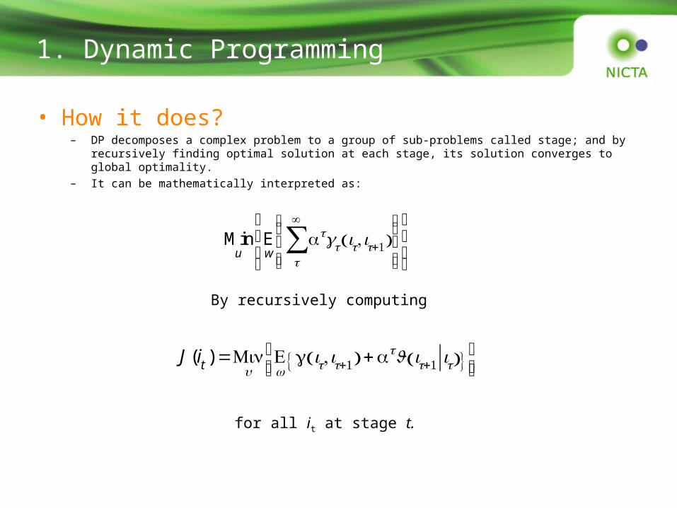
• How it does?– DP decomposes a complex problem to a group of sub-problems called stage; and by recursively

finding optimal solution at each stage, its solution converges to global optimality.– It can be mathematically interpreted as:

By recursively computing

J (it ) =Min

uEw

g it,it+1( ) +αtJ it+1 it( ){ }⎡⎣⎢

⎤⎦⎥

Minu

Ew

αtgt it,it+1( )t

∞

∑⎧⎨⎪

⎩⎪

⎫⎬⎪

⎭⎪

⎡

⎣

⎢⎢

⎤

⎦

⎥⎥

for all it at stage t.

2. Curse of Dimensionality

2. Curse of Dimensionality

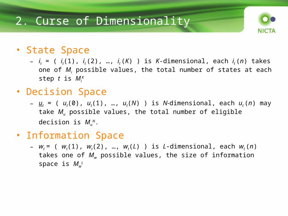
• State Space– it = ( it(1), it (2), …, it (K) ) is K-dimensional, each it (n) takes one of Mi possible values, the

total number of states at each step t is MiK

• Decision Space– ut = ( ut(0), ut(1), …, ut(N) ) is N-dimensional, each ut (n) may take Mu possible values, the

total number of eligible decision is MuN.

• Information Space– wt = ( wt(1), wt(2), …, wt(L) ) is L-dimensional, each wt (n) takes one of Mw possible values,

the size of information space is MwL

2. Curse of Dimensionality

1010 ×105 ×105 =1020

M iK ×Mw

L ×MuN

J (it ) =Min

uEw

g it,it+1( ) +αtJ it+1 it( ){ }⎡⎣⎢

⎤⎦⎥

• Three curses of dimensionality

• Computational demand is

In the case that K=10, L=5, and N=5, and MiK= Mw

L= MuN=10,

the total computational demand is

state

informationdecision

3. Approximate Dynamic Programming

3. Approximate Dynamic Programming

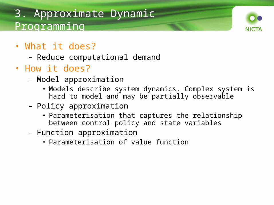
• What it does?– Reduce computational demand

• How it does?– Model approximation

• Models describe system dynamics. Complex system is hard to model and may be partially observable

– Policy approximation• Parameterisation that captures the relationship between

control policy and state variables– Function approximation

• Parameterisation of value function

3. Approximate Dynamic Programming

J (it ) =Min

uEw

gt it,it+1( ) +αtJ it+1( ){ }⎡⎣⎢

⎤⎦⎥

J (it ) =Min

uEw

gt it,it+1( ) +αt %J it+1,rt( ){ }⎡⎣⎢

⎤⎦⎥

( )( )

( )

1r

r k

r K

⎡ ⎤⎢ ⎥

= ⎢ ⎥⎢ ⎥⎣ ⎦

M

%J i,r( ) : X ×° K → °

J i( ) : X → °

• Parameterisation of value function

3. Approximate Dynamic Programming

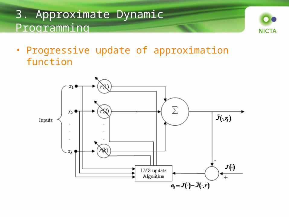
• Progressive update of approximation function

4. ADP in Adaptive Traffic Signal Control

4. Adaptive Traffic Signals

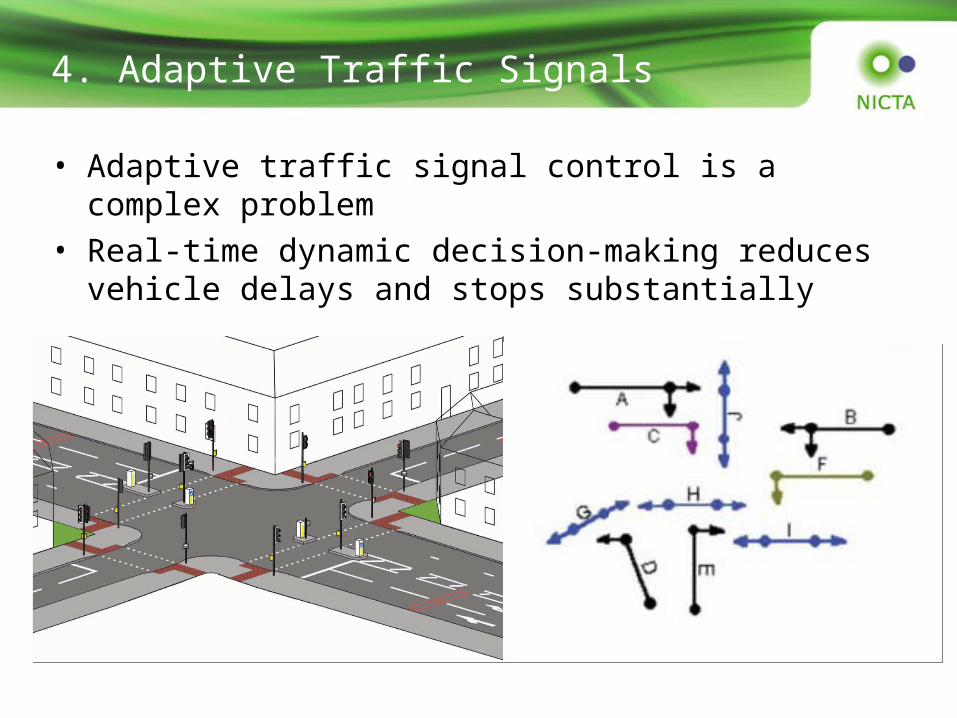
• Adaptive traffic signal control is a complex problem

• Real-time dynamic decision-making reduces vehicle delays and stops substantially

4. Adaptive Traffic Signals

QuickTime™ and a decompressor

are needed to see this picture.

QuickTime™ and a decompressor

are needed to see this picture.

QuickTime™ and a decompressor

are needed to see this picture.

QuickTime™ and a decompressor

are needed to see this picture.

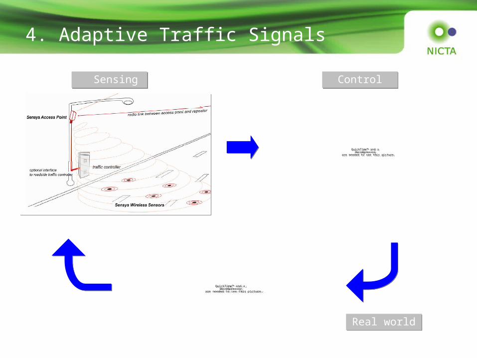
Sensing Sensing ControlControl

Real worldReal world

4. Adaptive Traffic Signals

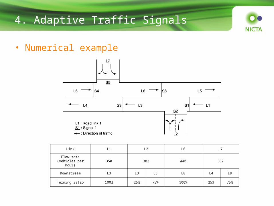
• Numerical example

Link L1 L2 L6 L7

Flow rate(vehicles per hour)

350 382 440 382

Downstream L3 L3 L5 L8 L4 L8

Turning ratio 100% 25% 75% 100% 25% 75%

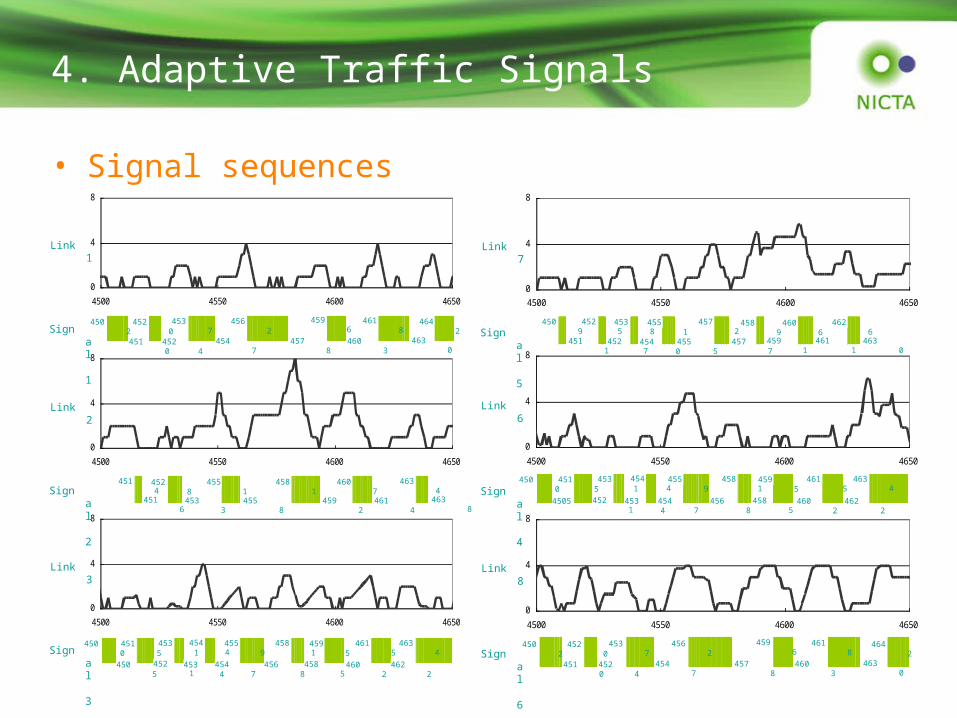
4. Adaptive Traffic Signals

• Signal sequences

Link 7

Signal 5

Link 6

Signal 4

0

4

8

4500 4550 4600 4650

Link 8

Signal 6

0

4

8

4500 4550 4600 4650

0

4

8

4500 4550 4600 4650

4505

4500451

5453

1

4521

4534

4568

4559

4547

4544

4634

4622

4615

4602

4595

4585

4581

4611

4555

4551

4540

4538

4527

4525

4511

4509

4606

4591

4589

4577

4572

4630

4626

4524

4520

4510

4502

4537

4596

4578

4562

4547

4630

4618

4603

4642

0

4

8

4500 4550 4600 4650

Link 1

Signal 1

0

4

8

4500 4550 4600 4650

Link 2

Signal 2

0

4

8

4500 4550 4600 4650

Link 3

Signal 3

4630

4642

4524

4520

4510

4502

4537

4596

4578

4562

4547

4618

4603

4505

4500451

5453

1

4521

4534

4568

4559

4547

4544

4634

4622

4615

4602

4595

4585

4581

4533

4516

4528

4514

4551

4607

4592

4581

4558

4634

4614

4638

4. Adaptive Traffic Signals

• Up to 60% reduction in vehicle delays in comparison with optimised fixed-time plans

• Fully adaptive and applicable to distributed network control

• Computation demand manageable by real-time systems

5. Conclusion

• Dynamic programming is the only exact solution to sequential decision-making for discrete systems

• DP is difficult for real-time control because of computational demand

• Approximation to DP can reduce dimensionality and therefore make problem-solving tractable

• ADP is a general framework in which various approximation architectures and machine learning techniques can be used

• Adaptive traffic signal controller using ADP demonstrated promising results in reducing vehicle delays

From imagination to impact