lable at ScienceDirect

Atmospheric Environment 80 (2013) 488e498

Contents lists avai

Atmospheric Environment

journal homepage: www.elsevier .com/locate/atmosenv

Chemical loss of volatile organic compounds and its impact on thesource analysis through a two-year continuous measurement

H.L. Wang a, C.H. Chen a, *, Q. Wang a, C. Huang a, L.Y. Su a, H.Y. Huang a, S.R. Lou a,M. Zhou a, L. Li a, L.P. Qiao a, Y.H. Wang b

a Shanghai Academy of Environmental Sciences, 508 Qinzhou Rd., Shanghai 200233, Chinab School of Earth and Atmospheric Science, Georgia Institute of Technology, Atlanta 30332, USA

h i g h l i g h t s

� 35% initial VOCs had been consumed during the transport from sources to the receptor.� Reactivity of VOCs was underestimated over 60% if the removal of VOCs was ignored.� C3eC5 alkenes and C8 aromatics contributed over 60% of the chemical loss of VOCs.� Seven sources of VOCs were identified and quantified in Shanghai urban.� The regional transportation contributed w20% of VOCs in Shanghai urban from PMF.

a r t i c l e i n f o

Article history:Received 19 February 2013Received in revised form19 August 2013Accepted 21 August 2013

Keywords:Volatile organic compoundsObserved VOCsChemical lossInitial VOCsSource analysis

* Corresponding author. Tel./fax: þ86 21 64085119xE-mail addresses: chench@saes.sh.cn, saeschen200

1352-2310/$ e see front matter � 2013 Elsevier Ltd.http://dx.doi.org/10.1016/j.atmosenv.2013.08.040

a b s t r a c t

Chemical loss of volatile organic compounds (VOCs) is more important than the observed VOCs, which isthe real actor of the chemical process in the atmosphere. The chemical loss of VOCs might impact on theidentification of VOCs sources in ambient. For this reason, VOCs with 56 species were continuouslymeasured in the urban area of Shanghai from 2009 to 2010, and based on the measurement the chemicalloss of VOCs was calculated. According to the result, the initial VOCs in Shanghai urban was (34.8 � 20.7)ppbv, higher than the observed one by w35%, including alkanes (w38%), aromatics (w36%), alkenes(w17%), and acetylene (w8%). The chemical reactivity of VOCs would be underestimated by w60% ifthe chemical loss were ignored. The chemical loss of VOCs showed a good agreement with Ox(O3 þ NO2). C7eC8 aromatics and C3eC5 alkenes contributed w60% of consumed VOCs. Seven sourceswere identified and quantified from positive matrix factorization (PMF) analysis. Vehicular emissionswere the largest anthropogenic source of VOCs in Shanghai urban, accounting for 27.6% of VOCs, followedby solvent usage (19.4%), chemical industry (13.2%), petrochemical industry (9.1%), and coal burning(w5%). The contribution of biogenic emissions to total VOCs was 5.8%. Besides the five local anthropo-genic sources and one biogenic source, the regional transportation was identified as one importantsource, contributing about 20% of VOCs in Shanghai urban. Sources apportionment results from PMFanalysis based on the initial VOCs showed some differences from those based on observed data andmight be more appropriate to be applied into the formulation of air pollution control measures.

� 2013 Elsevier Ltd. All rights reserved.

1. Introduction

Shanghai has been experiencing a rapid economic growth in thepast decades. The increase of the energy consumption due to therapid economic growth resulted in a dramatic increase of the pol-lutants emissions (Huang et al., 2011) and the deterioration of theair quality in Shanghai, in term of ozone and fine particles (Gao

2503.5@21cn.com (C.H. Chen).

All rights reserved.

et al., 2009; Geng et al., 2009; Tie and Cao, 2009). Volatileorganic compounds (VOCs) are important precursors of thephotochemical process and have been paid a large amount atten-tion to as their great contribution to the formation of troposphereozone and secondary organic aerosols (SOA) (IPCC, 2007; Seinfeldand Pandis, 2006).

So far, many studies have been conducted to investigate thecharacterization of VOCs and the key VOCs components of ozoneformation in Shanghai. However, identifying the important con-tributors to ozone formation potential (OFP) based solely on theobserved datawas problematic (Shao et al., 2011). The chemical loss

0 2 4 6 8 10

0

2

4

6

8

10

0 1 2 3 4 5

0

1

2

3

4

5

Alkene

Co

nc

en

tra

tio

n fro

m G

C-F

ID

, p

pb

v

Propane

n-Decane

n-Undecane

Ethane

Alkane

0 1 2 3 4 5

0

1

2

3

4

5

Propene

Ethylene

0 1 2 3 4 5

0

1

2

3

4

5

Aromatic

Reference concentration in standard gas, ppbv

m-Ethyltoluene

Diethylbenzene

2-2-Dime-Butane

2-3-DIMEC5+2MEC6

m,p-Xylenes

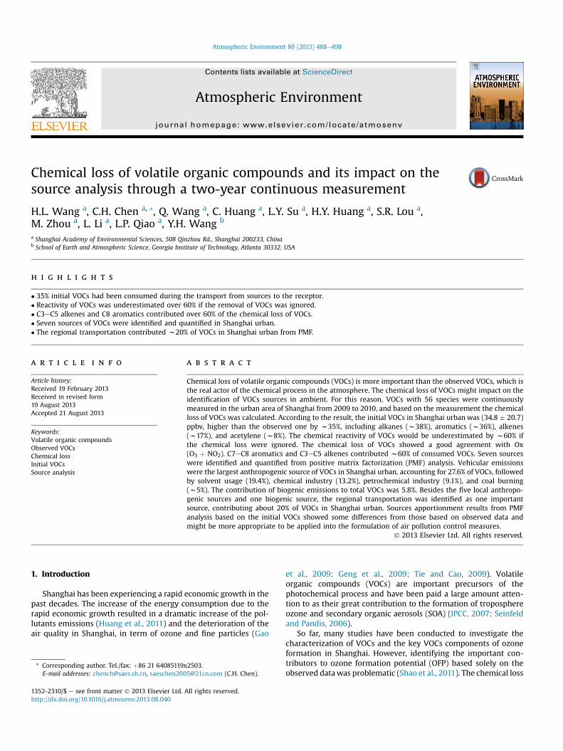
Fig. 1. Comparison of the manual calibration results and the reference concentrations in standard gas.

H.L. Wang et al. / Atmospheric Environment 80 (2013) 488e498 489

of the reactive VOC species during the transportation from emis-sion sources to the receptor site played important role in the for-mation of ozone. As studied by Xie et al. (2008), the chemical loss ofthe reactive VOC species contributed more than one third of theOFP in Beijing urban. Actually, the consumed VOCs might be thereal contributors to the ozone formation, which could not be takeninto account by the observed data. The oxidants formation agreedbetter with the consumption of VOCs than with the observed VOCsin Beijing during the 2008 Olympic period (Shao et al., 2011).Furthermore, the source apportionment of VOCs would have largeuncertainty for the reactive VOC species if the chemical loss wasignored (Wittig and Allen, 2008). The source apportionment ofVOCs by Chemical Mass Balance model (CMB) considering thechemical loss differed a lot from that based on the observed data(Na and Kim, 2007; Shao et al., 2011). As reported by Na and Kim(2007), the contribution from vehicle exhaust was under-estimated by 10%when the chemical loss effect was incorporated inthe CMB calculation while the contribution from solvent usage andgasoline evaporation were overestimated. Generally, the contribu-tion of sources with more reactive species would be under-estimated based on the observed VOCs.

There were usually two kinds of methods using to estimate theconsumption of VOCs in ambient. One was through estimating thephotochemical age of air mass by the VOC species pairs from thesame emission sources but having different reactivities with OH(McKeen et al., 1996). The other was based on the oxidation prod-ucts measurement to estimate the consumption of their parent VOCspecies (Bertman et al., 1995; Wiedinmeyer et al., 2001). Thechemical loss of VOCs has been estimated previously in differentregions (Shao et al., 2011; Shiu et al., 2007; Xie et al., 2008) but notin Shanghai.

In this study, the continuous measurement of C2eC12 VOCspecies were carried out for two years to investigate the charac-terization of VOCs in urban Shanghai, China. Based on the observeddata, the chemical loss of VOCs was estimated. The high responsetemporal variation of VOCs through over the two years was

discussed in detail combining with the oxidants variations in Sec-tions 3.2 and 3.3. Studies of VOCs in other cities were employed tocompare with that in this study, and some special result inShanghai was obtained in Section 3.4. According to the estimationresult of the chemical loss, the sources contributions were quan-tified by receptor model, positive matrix factorization (PMF)(Paatero, 1997), in Section 3.5. Finally, in Section 4, the conclusionsof the present study were summarized and the implications werediscussed.

2. Experiment

2.1. Monitoring sites

Themonitoring site locates in the southwest of the urban area inShanghai, China. It is about 8 km away from the city center. Thesample inlet is on the roof of a 5-floor building at Shanghai Acad-emy of Environmental Science (31.17�N, 121.43�E), about 15 mabove the ground. There are no other large VOCs sources except thevehicular and domestic emissions in the urban area. In the southand southwest around 50 km away from the monitoring site, thereare some petrochemical and chemical industrial factories in therural area (Cai et al., 2010; Huang et al., 2011), which may haveeffects on the VOCs measured results at the monitoring site in thespecial meteorological conditions.

2.2. Measurement of VOCs

Individual VOC species were continuously measured every30 min from January 2009 to December 2010 by two on-line highperformance gas chromatograph with flame ionization detector(GC-FID) systems (Chromato-sud airmoVOC C2eC6 #5250308 andairmoVOC C6eC12 #2260308, France). For C2eC6 VOCs, the sampleis preconcentrated through a trap, a fine tube containing poroussubstances. Three trap phases, including Carbotrap C, Carbopack Band Carboxen, are chosen so as to trap from the selected

H.L. Wang et al. / Atmospheric Environment 80 (2013) 488e498490

compounds. The trap is cooled by a cell with Peltier effect duringthe sampling. The temperature for the cold is set at�8 �C. Then, thetube is heated and thermodesorption is fixed at 220 �C, followed byseparation on an ultimetal column (id ¼ 0.53 mm, length: 25 m). Aflame ionization detector (FID) is used for quantification. The airsample volume for C2eC6 analysis is around 80 mL. For C6eC12VOCs, the sample is preconcentrated through a trap, and the trapphase (Carbotrap B) is chosen so as to trap C6eC12 compounds.Then, the thermodesorption is fixed to 380 �C, followed by sepa-ration on an ultimetal column (id ¼ 0.28 mm, length: 30 m, MXT30CE, 1 mm), and the detector is also FID. The air sample volume isaround 105 mL. This instrument includes one auto-calibration unit,which uses three internal permeation tubes with standard com-pounds, to make auto-calibration every 24 h. The detection limitsfor VOC species are between several tens to hundreds pptv (Liuet al., 2012).

Additionally, the manual calibration by standard gas (Spectra,USA) was also performed periodically. The measured results by GC-FID were used to compare with the reference concentrations of thestandard gas diluted by dynamic gas calibrator. Fig. 1 shows that forthe species of C2eC3, there were large differences between the tworesults, and the results from GC-FID were only half of the referenceconcentrations in standard gas. This was mainly because theadsorption efficiencies of C2eC3 species in the trapwere low due tothe high volatility of these species. By contrast, in terms of ethyl-toluene, diethylbenzene and n-undecane, their desorption effi-ciencies were low due to their low volatility, which resulted in theunderestimation of their concentrations by w30%, as shown inFig. 1. In addition, it seems that the correlation of n-decane had asignificant intercept, probably due to the high concentration of n-decane in zero gas. In this study, the measured concentrations of C3species and n-decane were recalculated according to their cali-bration curves, because the concentrations of these species inambient were considerable and meanwhile the measured resultsand the reference concentrations in standard gas had strong cor-relations (R2 > 0.99). The concentrations of ethane, ethylene, eth-yltoluene, diethylbenzene and n-undecane in this text were themeasured results from GC-FID. For the other 46 kinds of VOC spe-cies, the correlations between the measured results from GC-FIDand the reference concentrations in standard gas were good(R2> 0.99), and the average slope of the correlationwas 0.95� 0.10.

2.3. Estimation of the initial mixing ratio of VOCs

VOCs are usually composed of species with high chemicalreactivity, and their lifetimes range from several hours to severalhundred hours dependent on their reactivity and the concentrationof OH radical. For example, the chemical lifetime of isoprene is onlyw1 h in the condition of OH radical concentration of5.0 � 106 molecule cm�3, while the lifetime of propane is about100 h under the same condition. Consequently, the photochemicalloss of VOCs is more significant for the VOC species with larger OHreaction rate constant. The sum of chemical loss and the observedmixing ratio of VOC species was considered as the initial mixingratio.

Several methods used for calculating the initial mixing ratio ofVOCs have been developed previously (McKeen et al., 1996;Wiedinmeyer et al., 2001). In the study of Wiedinmeyer et al.(2001), VOCs initial mixing ratio was calculated according to theisoprene conversion process, using the observed data of isopreneand its oxidation products (Xie et al., 2008). Because the products ofisoprene were not observed from the measurements, we used themethod mentioned in McKeen et al. (1996) to calculate the initialmixing ratio of VOCs. General description of the method ismentioned as below.

The major loss of VOCs is assumed due to their reactions withOH radicals in daytime. To estimate the initial mixing ratio of theVOCs, two hydrocarbons from the same emission sources buthaving different reactivities with OH are generally used as a mea-sure of photochemical oxidation by OH radicals (de Gouw et al.,2005; Goldan et al., 2000; Jobson et al., 1999; McKeen and Liu,1993; Kramp and Volz-Thomas, 1997). In this study, we chooseethylbenzene (E) and m,p-xylenes (X), for this purpose (Nelson andQuigley, 1983). The initial mixing ratio can be calculated by theequations below (McKeen et al., 1996):

½VOCi�t ¼ ½VOCi�0 � expð � ki½OH�DtÞ (1)

Dt ¼ 1½OH�ðkE � kXÞ

��ln�½E�½X�

��t¼t0

�� ln

�½E�½X�

��t¼t

��(2)

Where [VOCi]t and [VOCi]0 are the observed and initial mixing ratioof VOCi, respectively. ki is the reaction rate constant of VOCiwith OHradicals, and kE and kX are the reaction rate constants of ethyl-benzene (E) and m,p-xylenes (X) with OH radicals. [OH] is themixing ratio of OH radicals. Dt is the reaction time or the photo-chemical age. It should be noted that these results do not dependon the OH mixing ratio assumed: if a lower value of [OH] isassumed, then the photochemical age according to Equation (2)increases, and the product [OH] Dt in Equation (1) remains thesame. ([E]/[X])t ¼ t0 is the ratio between the initial mixing ratios ofethylbenzene and m,p-xylenes, and in other words, is the ratio of[E] to [X] in the VOCs emission sources. ([E]/[X])t ¼ t is the ratio of[E] to [X] at time t. Given the assumption that the removal of VOCsis governed by the reactions with OH radicals, the initial mixingratios of VOCs were only estimated in daytime (i.e. 8:00e18:00) inthe present study.

As reported in the previous studies, the values of ([E]/[X])t ¼ t0for the sources related to the vehicular emission and the coalcombustion are 0.3e0.4 (Liu et al., 2008), and is around 0.4e0.5 forsolvent use (Wang et al., 2013; Yuan et al., 2010), and is about 0.65for the biomass burning (Liu et al., 2008), and for the petrochemicaland chemical processes this value is around 0.5e0.7 (Liu et al.,2008). According to the VOCs emission inventory in Shanghai, thepetrochemical and chemical processes, painting and printing andvehicle contributed more than 80% of VOCs in 2007 (Huang et al.,2011). Therefore, we chose the value of ([E]/[X])t ¼ t0 as 0.5 in thisstudy. In addition, higher (0.7) and lower (0.3) ([E]/[X])t ¼ t0 wereused to carried out the sensitivity analysis and to test the un-certainties of estimation of initial mixing ratios. As a result, therelative changes of initial mixing ratios of different species rangedfrom 5% to 122% and from 1% to �48% for lower and higher ([E]/[X])t ¼ t0, respectively. Generally, initial mixing ratios of reactiveVOC species were more sensitivity to ([E]/[X])t ¼ t0, and conse-quently their uncertainties were relatively high.

Additionally, the uncertainty of estimating the initial mixingratio by hydrocarbons ratio method has been pointed out previ-ously (McKeen and Liu, 1993). For example, the mixing of qualita-tively different air masses could also have similar effects aschemical reactions on the atmospheric composition (Parrish et al.,2007). McKeen et al. (1996) showed that the time for dilution withbackground air was about 2.5 days, which was longer than theprocesses focused on in this study. Nevertheless, the assumptionthat the effects of mixing could be ignored should be treated withsome caution.

In addition, there were some limitations for estimating initialmixing ratios of reactive species using the method above. de Gouwet al. (2005) estimated the rate coefficients for the reaction of allprimary anthropogenic VOCs with OH radical using the method

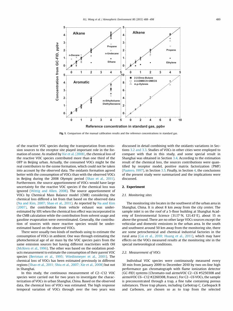
Fig. 2. Mixing ratio, LOH, and the OFP of each chemical VOC group in 2009 and 2010(Obs-N: the observed mixing ratio during nighttime, Obs-D: the observed mixing ratioduring daytime, Ini-D: the initial mixing ratio during daytime.).

H.L. Wang et al. / Atmospheric Environment 80 (2013) 488e498 491

above by the ratios of toluene/benzene and o-xylene/toluene, andfound that their results agreed well with the literature rate co-efficients until the rate coefficient of toluene (in the case of usingtoluene/benzene ratio) or o-xylene (in the case of using toluene/o-xylene). For the VOC species with faster removal than that oftoluene (in the case of using toluene/benzene ratio) or o-xylene (inthe case of using toluene/o-xylene), the rate coefficients becameconstant according to de Gouw et al. (2005) results, and the ratecoefficients of alkenes were determined with large uncertainties as

their small observed mixing ratios and very fast removal processes.Given that, for the VOC species with larger rate coefficients thanthat of m,p-xylene, their initial mixing ratios were estimated usingthe rate coefficient of m,p-xylene in Equation (1) rather thanthemselves’ in this study. Therefore, the initial mixing ratio ofreactive species obtained in this study was a lower estimate.

3. Results and discussion

3.1. Characteristics of VOCs

3.1.1. Mixing ratioFig. 2 summarized the observed and initial mixing ratios of each

chemical VOC groups both in 2009 and 2010. In order to betterunderstand the difference between the observed and the initialmixing ratio of each group, we divided the observed data into twogroups, i.e. daytime (8:00e18:00) and nighttime (0:00e7:00 and19:00e23:00). The observed mixing ratios of total VOCs (TVOC)during nighttime were (30.8 � 21.2) ppbv in 2009 and (28.7� 21.5)ppbv in 2010 averaged daily, respectively, compared to (26.4�16.0)ppbv and (24.5 � 13.6) ppbv, respectively during daytime, mainlydue to the lower height of mixing layer during night. The initialmixing ratios of TVOC during daytime were (35.4 � 21.6) ppbv in2009 and (34.1 � 19.8) ppbv in 2010, respectively, higher than theobserved ones by w35%. A larger amount of VOCs had beenconsumed in atmosphere before measured.

According to the observed data, alkanes were the largest groupof VOCs, with a mixing ratio around (12.9 � 8.1) ppbv, followed byaromatics ((8.7 � 6.2) ppbv), alkenes ((3.6 � 2.6) ppbv) and acet-ylene ((2.5 � 1.9) ppbv). Further examination showed that toluene,acetylene and C2eC3 alkanes were the most abundant species,accounting for more than w35% of the total observed VOCs, fol-lowed by C8 aromatics and C4eC5 alkanes. C2eC3 alkeneswere thelargest composition of observed alkenes. These VOC species arealmost related to the traffic emission (Liu et al., 2008), and indus-trial processes such as solvent usage are also important sources oftoluene and C8 aromatics (Yuan et al., 2010).

Compared to the speciation of observed VOCs in daytime, thecontribution of reactive VOC species to the initial VOCs was higher.The contributions of aromatics and alkenes to initial VOCsincreased to w36% and w17%, and especially the proportion of C8aromatics, toluene, and C2eC3 alkenes were more than 40% of theinitial VOCs, followed by C4eC5 alkenes. Correspondingly, theproportion of alkanes and acetylene decreased to about w38% andw8% in initial mixing ratio of VOCs.

3.1.2. Reactivity: the OH loss rate and the ozone formation potentialThe OH loss rate (LOH) and OFP of each VOC species was calcu-

lated to evaluate the VOC reactivity combining with the constant ofOH loss rate (kOH) and maximum incremental reactivity (MIR)(Atkinson et al., 2006; Carter, 2008). The average reactivity of VOCswas calculated as the ratio of the total LOH or OFP to the mixingratio.

For the reactivity of observed VOCs, no significant differenceswere observed between 2009 and 2010. The total LOH in these twoyears was w6 s�1, and the OFP was w120 ppbv. The reactivityduring nighttimewas higher than that in daytime byw20% for bothLOH and OFP, mainly because of the higher mixing ratio of VOCs innighttime. The average kOH and MIR were8.7 � 10�12 cm3 molecule�1 s�1 and 4.2 (mol O3/mol VOCs),respectively. These values are comparable to those of ethylene(Atkinson et al., 2006; Carter, 2008), respectively.

In the case of the initial reactivity, the total LOH in these twoyears was w10 s�1 and the OFP was w186 ppbv. Compared to theobserved reactivity in daytime, the initial LOH and OFP increased by

H.L. Wang et al. / Atmospheric Environment 80 (2013) 488e498492

67% and 55%, respectively. The average kOH and MIR of the initialVOCs was 11.6 � 10�12 cm3 molecule�1 s�1 and 5.4 (mol O3/molVOCs), respectively. Most of the increment resulted from alkenesand aromatics as indicated in Fig. 2.

Further examination showed that the largest contributing spe-cies to LOH were C4eC5 alkenes, C8 aromatics, C2eC3 alkenes andtoluene. These species took up about 75% of the total LOH ofobserved VOCs and this proportion increased to 81% for the initialLOH. Specifically, C4eC5 alkenes and C8 aromatics contributedabout 44% and 26% of the increment part (LOH of consumed VOCs),followed by C2eC3 alkenes (14%). In the case of OFP, C8 aromaticsand toluene contributed 48% of the observed OFP, followed by al-kenes. The contribution of these reactive species to the initial VOCsOFP increased at different extent dependent on their reactivities.Most of the increment OFP was attributed to C8 aromatics (44%),and toluene and the other aromatics accounted for 22%, followed byC4eC5 and C2eC3 alkenes.

3.2. Monthly variations

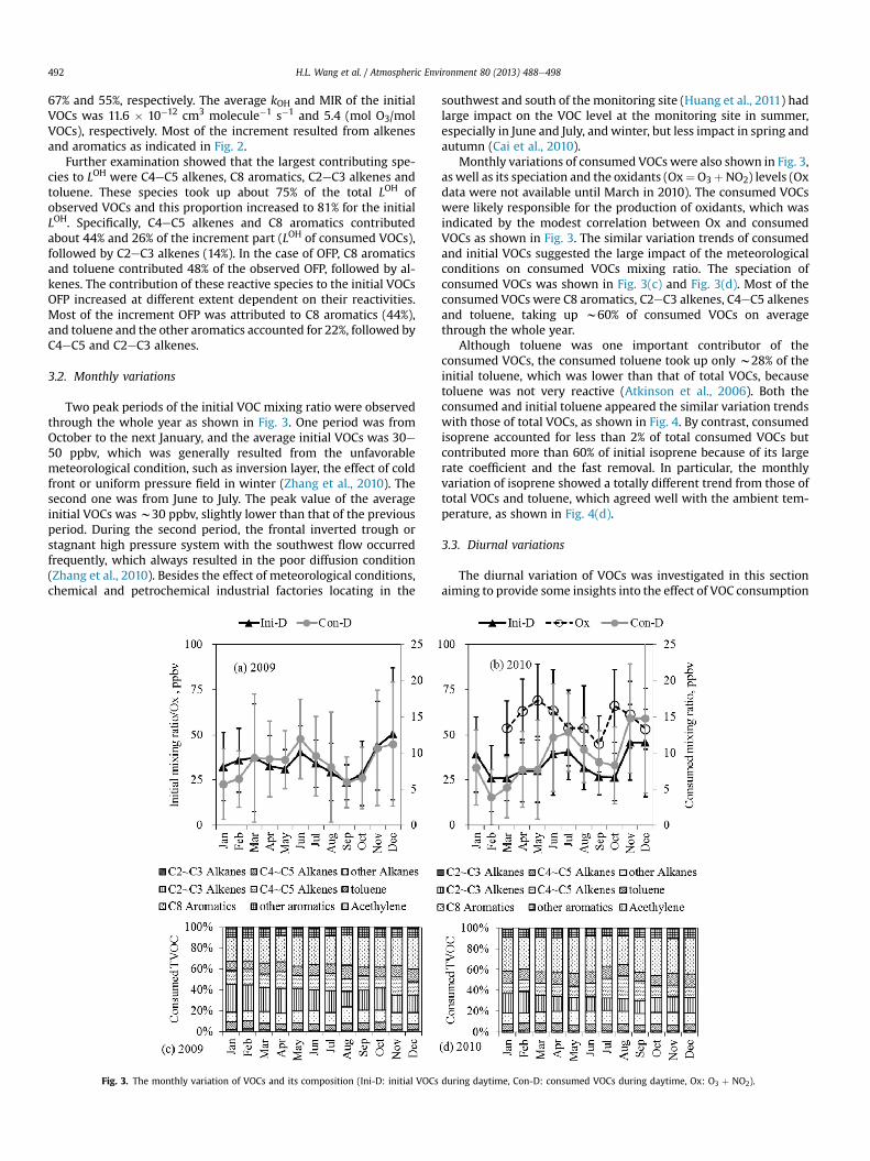
Two peak periods of the initial VOC mixing ratio were observedthrough the whole year as shown in Fig. 3. One period was fromOctober to the next January, and the average initial VOCs was 30e50 ppbv, which was generally resulted from the unfavorablemeteorological condition, such as inversion layer, the effect of coldfront or uniform pressure field in winter (Zhang et al., 2010). Thesecond one was from June to July. The peak value of the averageinitial VOCs was w30 ppbv, slightly lower than that of the previousperiod. During the second period, the frontal inverted trough orstagnant high pressure system with the southwest flow occurredfrequently, which always resulted in the poor diffusion condition(Zhang et al., 2010). Besides the effect of meteorological conditions,chemical and petrochemical industrial factories locating in the

Fig. 3. The monthly variation of VOCs and its composition (Ini-D: initial VOCs

southwest and south of the monitoring site (Huang et al., 2011) hadlarge impact on the VOC level at the monitoring site in summer,especially in June and July, and winter, but less impact in spring andautumn (Cai et al., 2010).

Monthly variations of consumed VOCs were also shown in Fig. 3,as well as its speciation and the oxidants (Ox¼O3þNO2) levels (Oxdata were not available until March in 2010). The consumed VOCswere likely responsible for the production of oxidants, which wasindicated by the modest correlation between Ox and consumedVOCs as shown in Fig. 3. The similar variation trends of consumedand initial VOCs suggested the large impact of the meteorologicalconditions on consumed VOCs mixing ratio. The speciation ofconsumed VOCs was shown in Fig. 3(c) and Fig. 3(d). Most of theconsumed VOCs were C8 aromatics, C2eC3 alkenes, C4eC5 alkenesand toluene, taking up w60% of consumed VOCs on averagethrough the whole year.

Although toluene was one important contributor of theconsumed VOCs, the consumed toluene took up only w28% of theinitial toluene, which was lower than that of total VOCs, becausetoluene was not very reactive (Atkinson et al., 2006). Both theconsumed and initial toluene appeared the similar variation trendswith those of total VOCs, as shown in Fig. 4. By contrast, consumedisoprene accounted for less than 2% of total consumed VOCs butcontributed more than 60% of initial isoprene because of its largerate coefficient and the fast removal. In particular, the monthlyvariation of isoprene showed a totally different trend from those oftotal VOCs and toluene, which agreed well with the ambient tem-perature, as shown in Fig. 4(d).

3.3. Diurnal variations

The diurnal variation of VOCs was investigated in this sectionaiming to provide some insights into the effect of VOC consumption

during daytime, Con-D: consumed VOCs during daytime, Ox: O3 þ NO2).

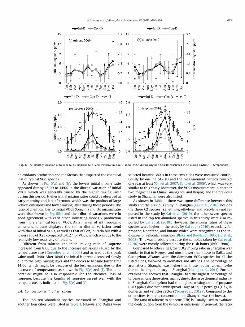
Fig. 4. The monthly variation of toluene (a, b), isoprene (c, d) and temperature (Ini-D: initial VOCs during daytime, Con-D: consumed VOCs during daytime, T: temperature).

H.L. Wang et al. / Atmospheric Environment 80 (2013) 488e498 493

on oxidants production and the factors that impacted the chemicalloss of typical VOC species.

As shown in Fig. 5(a) and (b), the lowest initial mixing ratioappeared during 13:00 to 14:00 in the diurnal variation of initialVOCs, which was generally caused by the higher mixing layerduring this period. Higher initial mixing ratios could be observed atearly morning and late afternoon, which was the product of largevehicle emissions and lower mixing layer during these periods. Theratio of chemical loss to initial VOCs (Con/Ini) and Ox mixing ratiowere also shown in Fig. 5(b), and their diurnal variations were ingood agreement with each other, indicating more Ox productionfrom more chemical loss of VOCs. As a marker of anthropogenicemissions, toluene displayed the similar diurnal variation trendwith that of initial VOCs, as well as that of Con/Ini ratio but with alower ratio of 0.23 compared to 0.27 for VOCs, which was due to therelatively low reactivity of toluene.

Different from toluene, the initial mixing ratio of isopreneincreased from 8:00 due to the increase emissions caused by thetemperature rise (Guenther et al., 2006) and arrived at the peakvalue until 10:00. After 10:00 the initial isoprene decreased slowlydue to the high mixing layer and the decrease became faster after14:00, which might be because of the less emissions due to thedecrease of temperature, as shown in Fig. 5(e) and (f). The tem-perature might be also responsible for the chemical loss ofisoprene, because the Con/Ini of isoprene agreed well with thetemperature, as indicated in Fig. 5(e) and (f).

3.4. Comparison with other regions

The top ten abundant species measured in Shanghai andanother four cities were listed in Table 1. Nagoya and Dallas were

selected because VOCs in these two cities were measured contin-uously by on-line GC-FID and the measurement periods coveredone year at least (Qin et al., 2007; Saito et al., 2009), which was verysimilar to this study. Moreover, the VOCs measurement in anothertwo megacities in China, Guangzhou and Beijing, and the previousstudy in Shanghai were also listed.

As shown in Table 1, there was some difference between thisstudy and the previous study in Shanghai (Cai et al., 2010). Besidesthe three C2 species (i.e. ethane, ethylene, and acetylene) not re-ported in the study by Cai et al. (2010), the other seven specieslisted in the top ten abundant species in this study were also re-ported by Cai et al. (2010). However, the mixing ratios of thesespecies were higher in the study by Cai et al. (2010), especially forpropane, i-pentane, and butane which were recognized as the in-dicators of vehicular emission (Blake and Rowland, 1995; Liu et al.,2008). This was probably because the samples taken by Cai et al.(2010) were mostly collected during the rush hours (6:00e9:00).

Compared to other cities, the VOCs mixing ratio in Shanghai wassimilar to that in Nagoya, and much lower than those in Dallas andGuangzhou. Alkanes were the dominant VOCs species for all thelisted cities, followed by aromatics and alkenes. The percentage ofaromatics in Shanghai was higher than those in other cities, maybedue to the large industry in Shanghai (Huang et al., 2011). Furtherexamination showed that Shanghai had the highest percentage oftolueneamong these cities,mainlydue to the large chemical industryin Shanghai; Guangzhou had the highest mixing ratio of propane(6.83 ppbv), due to thewidespread usage of liquid petrol gas (LPG) indomestic and vehicles sectors (Yuan et al., 2012a). Compared to theother cities, isoprene concentration in Shanghai was the lowest.

The ratio of toluene to benzene (T/B) is usually used to evaluatethe contribution from the vehicular emissions. In general, the ratio

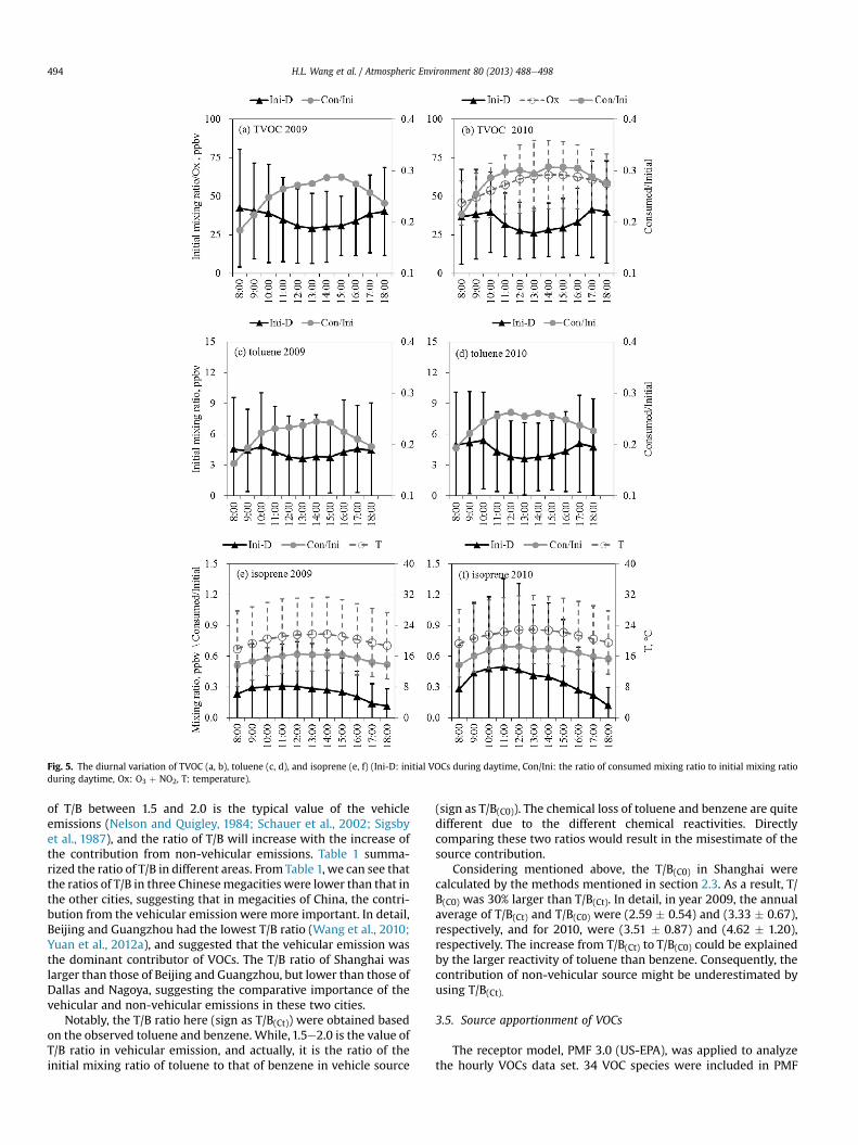
Fig. 5. The diurnal variation of TVOC (a, b), toluene (c, d), and isoprene (e, f) (Ini-D: initial VOCs during daytime, Con/Ini: the ratio of consumed mixing ratio to initial mixing ratioduring daytime, Ox: O3 þ NO2, T: temperature).

H.L. Wang et al. / Atmospheric Environment 80 (2013) 488e498494

of T/B between 1.5 and 2.0 is the typical value of the vehicleemissions (Nelson and Quigley, 1984; Schauer et al., 2002; Sigsbyet al., 1987), and the ratio of T/B will increase with the increase ofthe contribution from non-vehicular emissions. Table 1 summa-rized the ratio of T/B in different areas. From Table 1, we can see thatthe ratios of T/B in three Chinesemegacities were lower than that inthe other cities, suggesting that in megacities of China, the contri-bution from the vehicular emission were more important. In detail,Beijing and Guangzhou had the lowest T/B ratio (Wang et al., 2010;Yuan et al., 2012a), and suggested that the vehicular emission wasthe dominant contributor of VOCs. The T/B ratio of Shanghai waslarger than those of Beijing and Guangzhou, but lower than those ofDallas and Nagoya, suggesting the comparative importance of thevehicular and non-vehicular emissions in these two cities.

Notably, the T/B ratio here (sign as T/B(Ct)) were obtained basedon the observed toluene and benzene. While, 1.5e2.0 is the value ofT/B ratio in vehicular emission, and actually, it is the ratio of theinitial mixing ratio of toluene to that of benzene in vehicle source

(sign as T/B(C0)). The chemical loss of toluene and benzene are quitedifferent due to the different chemical reactivities. Directlycomparing these two ratios would result in the misestimate of thesource contribution.

Considering mentioned above, the T/B(C0) in Shanghai werecalculated by the methods mentioned in section 2.3. As a result, T/B(C0) was 30% larger than T/B(Ct). In detail, in year 2009, the annualaverage of T/B(Ct) and T/B(C0) were (2.59 � 0.54) and (3.33 � 0.67),respectively, and for 2010, were (3.51 � 0.87) and (4.62 � 1.20),respectively. The increase from T/B(Ct) to T/B(C0) could be explainedby the larger reactivity of toluene than benzene. Consequently, thecontribution of non-vehicular source might be underestimated byusing T/B(Ct).

3.5. Source apportionment of VOCs

The receptor model, PMF 3.0 (US-EPA), was applied to analyzethe hourly VOCs data set. 34 VOC species were included in PMF

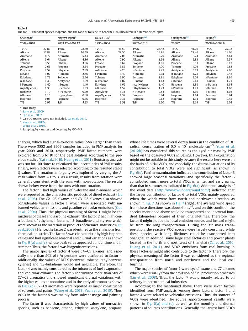
Table 1The top 10 abundant species, isoprene, and the ratio of toluene to benzene (T/B) measured in different cities, ppbv.

Shanghaia Nagoya Japanb Dallas USAc Shanghaid,g Guangzhoue,g Beijingf,g

2009e2010 2003.12e2004.12 1996e2004 2007e2010 2006.7 2008.6e2008.9

TVOC 27.82 TVOC 28.60 TVOC 41.50 TVOC 25.42 TVOC 41.26 TVOC 27.38Alkane 12.82 Alkane 16.59 Alkane 29.50 Alkane 13.91 Alkane 22.46 Alkane 14.66Aromatic 8.72 Aromatic 5.43 Aromatic 7.06 Aromatic 9.70 Aromatic 8.24 Aromatic 4.63Alkene 3.64 Alkene 4.86 Alkene 2.90 Alkene 1.94 Alkene 6.83 Alkene 5.37Toluene 3.53 Ethane 3.86 Ethane 6.62 Propane 4.81 Propane 6.83 Ethane 3.17Acetylene 2.63 Propane 3.34 Propane 5.82 Toluene 4.70 Toluene 4.03 Propane 2.82Propane 2.52 Ethylene 2.89 n-Butane 4.26 i-Pentane 2.29 Acetylene 3.73 Acetylene 2.80Ethane 1.92 n-Butane 2.66 i-Pentane 3.49 n-Butane 2.03 n-Butane 3.72 Ethylene 2.42Ethylene 1.73 Toluene 2.54 Toluene 2.90 Benzene 1.81 Ethylene 3.08 i-Pentane 1.99n-Butane 1.46 Acetylene 1.99 n-Pentane 1.87 i-Butane 1.43 i-Butane 2.43 Toluene 1.71i-Pentane 1.40 i-Butane 1.40 Ethylene 1.66 m,p-Xylenes 1.40 Benzene 1.84 n-Butane 1.68m,p-Xylenes 1.38 i-Pentane 1.33 i-Butane 1.57 Ethylbenzene 1.23 i-Pentane 1.73 i-Butane 1.60Benzene 1.19 n-Pentane 0.70 Acetylene 1.33 n-Hexane 0.84 Ethane 1.60 1-Bitene 1.08i-Butane 1.15 m,p-Xylenes 0.68 m,p-Xylenes 1.32 Propene 0.84 Isoprene 1.14 Benzene 0.84Isoprene 0.08 Isoprene 0.66 Isoprene 0.33 Isoprene 0.12 Isoprene 1.14 Isoprene 0.48T/B 2.97 T/B 5.23 T/B 3.58 T/B 2.60 T/B 2.19 T/B 2.04

a This study.b Saito et al., 2009.c Qin et al., 2007.d C2 VOC species were not included, Cai et al., 2010.e Yuan et al., 2012a.f Wang et al., 2010.g Sampling by canister and detecting by GCeMS.

H.L. Wang et al. / Atmospheric Environment 80 (2013) 488e498 495

analysis, which had signal-to-noise ratios (SNR) larger than three.There were 3552 and 3906 samples included in PMF analysis foryear 2009 and 2010, respectively. PMF factor numbers wereexplored from 5 to 10 for the best solution according to the pre-vious studies (Cai et al., 2010; Huang et al., 2011). Bootstrap analysiswas run for 100 times to calculated the uncertainties of PMF results.Finally, seven factors were selected according to the resulted stableQ values. The rotation ambiguity was explored by varying the F-Peak values from �3 to 3. As a result, results from rotation weregenerally consistent with the runs with non-rotation. The resultsshown below were from the runs with non-rotation.

The factor 1 had high values of n-decane and n-nonane whichwere reported as the characteristic products of diesel exhaust (Liuet al., 2008). The C2eC6 alkanes and C3eC5 alkenes also showedconsiderable values in factor 1, which were associated with un-burned vehicular emissions and gasoline vehicular emissions (Guoet al., 2004). Thus, the physical meaning of factor 1 might be themixtures of diesel and gasoline exhaust. The factor 2 had high con-tributions of ethylene, 1-butene, 1,3-butadiene and styrene whichwere known as thematerials or products of chemical industries (Liuet al., 2008). Hence, the factor 2was identified as the emissions fromchemical industries. The factor 3was characteristic by high isoprenevalues and had significant seasonal and diurnal variations as shownin Fig. 6 (a) and (c), whose peak value appeared at noontime and insummer. Thus, the factor 3 was biogenic emissions.

The major species of factor 4 were C4eC5 alkanes, and espe-cially more than 50% of i-/n-pentane were attributed to factor 4.Additionally, the values of BTEX (benzene, toluene, ethylbenzene,xylenes) and 1,3-butadiene would not negligible. Therefore, thefactor 4 was mainly considered as the mixtures of fuel evaporationand vehicular exhaust. The factor 5 contributed more than 50% ofC7eC9 aromatics and showed significant diurnal variations withthe higher values at noontime and in the early afternoon as shownin Fig. 6(c). C7eC9 aromatics were reported as major constituentsof solvents and paints (Wang et al., 2013; Yuan et al., 2010). Thus,VOCs in the factor 5 was mainly from solvent usage and paintingprocess.

The factor 6 was characteristic by high values of unreactivespecies, such as benzene, ethane, ethylene, acetylene, propane,

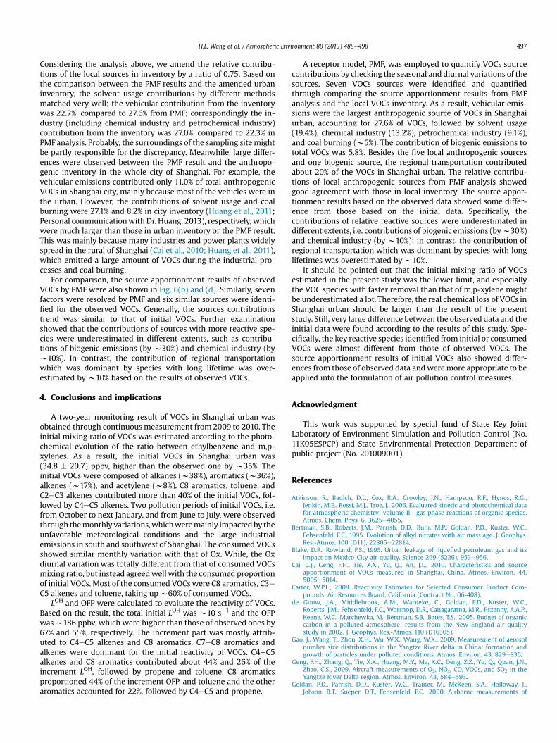
whose life times were several dozen hours in the condition of OHradical concentration of 5.0 � 106 molecule cm�3. Yuan et al.(2012b) has considered this source as the aged air mass by PMFbased on the observed VOCs in Beijing. However, this explanationmight not be suitable in this study because the results herewere onthe basis of initial VOCs, and especially, the diurnal variations of itscontribution to total VOCs were not significant, as shown inFig. 6(c). Further examination indicated the contribution of factor 6showed large seasonal variations, and specifically the factor 6contributed much more to total VOCs in winter and early springthan that in summer, as indicated in Fig. 6(a). Additional analysis ofthe wind data (http://www.wunderground.com/) indicated thatthe larger contribution of factor 6 to total VOCs mainly appearedwhen the winds were from north and northwest direction, asshown in Fig. 7. As shown in Fig. 7 (right), the average wind speedfrom these directions was about 6 m s�1, and on this condition thespecies mentioned above could be transported about several hun-dred kilometers because of their long lifetimes. Therefore, thefactor 6 might not be the local emission source, and instead mightbe from the long transportation. During the air mass trans-portation, the reactive VOC species were largely consumed whilethese species with long lifetimes could be transported intoShanghai. In addition, some large steel factories and power plantslocated in the north and northwest of Shanghai (Cai et al., 2010;Huang et al., 2011), and VOCs emissions from coal burning inthese factories might also contribute to the factor 6. Therefore, thephysical meaning of the factor 6 was considered as the regionaltransportation from north and northwest and the local coalburning.

The major species of factor 7 were cyclohexane and C7 alkaneswhich were usually from the emission of fuel production processes(Liu et al., 2008). Thus, the factor 7 was primarily related to oilrefinery in petrochemical industries.

According to the mentioned above, there were seven factorsidentified from PMF analysis. Among these factors, factor 1 andfactor 4 were related to vehicular emissions. Thus, six sources ofVOCs were identified. The source apportionment results wereshown in Fig. 6(a) and (c), as well as the monthly and diurnalpatterns of sources contributions. Generally, the largest local VOCs

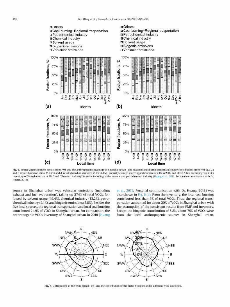
Fig. 6. Source apportionment results from PMF and the anthropogenic inventory in Shanghai urban (a,b), seasonal and diurnal patterns of source contributions from PMF (c,d). aand c, results based on initial VOCs; b and d, results based on observed VOCs; A-PMF, annually average source apportionment results in 2009 and 2010; A-Inv, anthropogenic VOCsinventory of Shanghai urban in 2010 and “Chemical industry” in A-Inv including both chemical and petrochemical industry (Huang et al., 2011; Personal communication with Dr.Huang, 2013).

H.L. Wang et al. / Atmospheric Environment 80 (2013) 488e498496

source in Shanghai urban was vehicular emissions (includingexhaust and fuel evaporation), taking up 27.6% of total VOCs, fol-lowed by solvent usage (19.4%), chemical industry (13.2%), petro-chemical industry (9.1%), and biogenic emissions (5.8%). Besides thefive local sources, the regional transportation and local coal burningcontributed 24.9% of VOCs in Shanghai urban. For comparison, theanthropogenic VOCs inventory of Shanghai urban in 2010 (Huang

Fig. 7. Distributions of the wind speed (left) and the contribut

et al., 2011; Personal communication with Dr. Huang, 2013) wasalso shown in Fig. 6 (a). From the inventory, the local coal burningcontributed less than 5% of total VOCs. Thus, the regional trans-portation accounted for about 20% of VOCs in Shanghai urban withthe assumption of the consistent results from PMF and inventory.Except the biogenic contribution of 5.8%, about 75% of VOCs werefrom the local anthropogenic sources in Shanghai urban.

ion of the factor 6 (right) under different wind directions.

H.L. Wang et al. / Atmospheric Environment 80 (2013) 488e498 497

Considering the analysis above, we amend the relative contribu-tions of the local sources in inventory by a ratio of 0.75. Based onthe comparison between the PMF results and the amended urbaninventory, the solvent usage contributions by different methodsmatched very well; the vehicular contribution from the inventorywas 22.7%, compared to 27.6% from PMF; correspondingly the in-dustry (including chemical industry and petrochemical industry)contribution from the inventory was 27.0%, compared to 22.3% inPMF analysis. Probably, the surroundings of the sampling sitemightbe partly responsible for the discrepancy. Meanwhile, large differ-ences were observed between the PMF result and the anthropo-genic inventory in the whole city of Shanghai. For example, thevehicular emissions contributed only 11.0% of total anthropogenicVOCs in Shanghai city, mainly because most of the vehicles were inthe urban. However, the contributions of solvent usage and coalburning were 27.1% and 8.2% in city inventory (Huang et al., 2011;Personal communicationwith Dr. Huang, 2013), respectively, whichwere much larger than those in urban inventory or the PMF result.This was mainly because many industries and power plants widelyspread in the rural of Shanghai (Cai et al., 2010; Huang et al., 2011),which emitted a large amount of VOCs during the industrial pro-cesses and coal burning.

For comparison, the source apportionment results of observedVOCs by PMF were also shown in Fig. 6(b) and (d). Similarly, sevenfactors were resolved by PMF and six similar sources were identi-fied for the observed VOCs. Generally, the sources contributionstrend was similar to that of initial VOCs. Further examinationshowed that the contributions of sources with more reactive spe-cies were underestimated in different extents, such as contribu-tions of biogenic emissions (by w30%) and chemical industry (byw10%). In contrast, the contribution of regional transportationwhich was dominant by species with long lifetime was over-estimated by w10% based on the results of observed VOCs.

4. Conclusions and implications

A two-year monitoring result of VOCs in Shanghai urban wasobtained through continuous measurement from 2009 to 2010. Theinitial mixing ratio of VOCs was estimated according to the photo-chemical evolution of the ratio between ethylbenzene and m,p-xylenes. As a result, the initial VOCs in Shanghai urban was(34.8 � 20.7) ppbv, higher than the observed one by w35%. Theinitial VOCs were composed of alkanes (w38%), aromatics (w36%),alkenes (w17%), and acetylene (w8%). C8 aromatics, toluene, andC2eC3 alkenes contributed more than 40% of the initial VOCs, fol-lowed by C4eC5 alkenes. Two pollution periods of initial VOCs, i.e.from October to next January, and from June to July, were observedthrough themonthly variations,whichweremainly impactedby theunfavorable meteorological conditions and the large industrialemissions in south and southwest of Shanghai. The consumed VOCsshowed similar monthly variation with that of Ox. While, the Oxdiurnal variation was totally different from that of consumed VOCsmixing ratio, but instead agreedwell with the consumed proportionof initial VOCs. Most of the consumed VOCs were C8 aromatics, C3eC5 alkenes and toluene, taking up w60% of consumed VOCs.

LOH and OFP were calculated to evaluate the reactivity of VOCs.Based on the result, the total initial LOH was w10 s�1 and the OFPwasw186 ppbv, which were higher than those of observed ones by67% and 55%, respectively. The increment part was mostly attrib-uted to C4eC5 alkenes and C8 aromatics. C7eC8 aromatics andalkenes were dominant for the initial reactivity of VOCs. C4eC5alkenes and C8 aromatics contributed about 44% and 26% of theincrement LOH, followed by propene and toluene. C8 aromaticsproportioned 44% of the increment OFP, and toluene and the otheraromatics accounted for 22%, followed by C4eC5 and propene.

A receptor model, PMF, was employed to quantify VOCs sourcecontributions by checking the seasonal and diurnal variations of thesources. Seven VOCs sources were identified and quantifiedthrough comparing the source apportionment results from PMFanalysis and the local VOCs inventory. As a result, vehicular emis-sions were the largest anthropogenic source of VOCs in Shanghaiurban, accounting for 27.6% of VOCs, followed by solvent usage(19.4%), chemical industry (13.2%), petrochemical industry (9.1%),and coal burning (w5%). The contribution of biogenic emissions tototal VOCs was 5.8%. Besides the five local anthropogenic sourcesand one biogenic source, the regional transportation contributedabout 20% of the VOCs in Shanghai urban. The relative contribu-tions of local anthropogenic sources from PMF analysis showedgood agreement with those in local inventory. The source appor-tionment results based on the observed data showed some differ-ence from those based on the initial data. Specifically, thecontributions of relative reactive sources were underestimated indifferent extents, i.e. contributions of biogenic emissions (byw30%)and chemical industry (by w10%); in contrast, the contribution ofregional transportation which was dominant by species with longlifetimes was overestimated by w10%.

It should be pointed out that the initial mixing ratio of VOCsestimated in the present study was the lower limit, and especiallythe VOC species with faster removal than that of m,p-xylene mightbe underestimated a lot. Therefore, the real chemical loss of VOCs inShanghai urban should be larger than the result of the presentstudy. Still, very large difference between the observed data and theinitial data were found according to the results of this study. Spe-cifically, the key reactive species identified from initial or consumedVOCs were almost different from those of observed VOCs. Thesource apportionment results of initial VOCs also showed differ-ences from those of observed data andweremore appropriate to beapplied into the formulation of air pollution control measures.

Acknowledgment

This work was supported by special fund of State Key JointLaboratory of Environment Simulation and Pollution Control (No.11K05ESPCP) and State Environmental Protection Department ofpublic project (No. 201009001).

References

Atkinson, R., Baulch, D.L., Cox, R.A., Crowley, J.N., Hampson, R.F., Hynes, R.G.,Jenkin, M.E., Rossi, M.J., Troe, J., 2006. Evaluated kinetic and photochemical datafor atmospheric chemistry: volume IIdgas phase reactions of organic species.Atmos. Chem. Phys. 6, 3625e4055.

Bertman, S.B., Roberts, J.M., Parrish, D.D., Buhr, M.P., Goldan, P.D., Kuster, W.C.,Fehsenfeld, F.C., 1995. Evolution of alkyl nitrates with air mass age. J. Geophys.Res.-Atmos. 100 (D11), 22805e22814.

Blake, D.R., Rowland, F.S., 1995. Urban leakage of liquefied petroleum gas and itsimpact on Mexico-City air-quality. Science 269 (5226), 953e956.

Cai, C.J., Geng, F.H., Tie, X.X., Yu, Q., An, J.L., 2010. Characteristics and sourceapportionment of VOCs measured in Shanghai, China. Atmos. Environ. 44,5005e5014.

Carter, W.P.L., 2008. Reactivity Estimates for Selected Consumer Product Com-pounds. Air Resources Board, California (Contract No. 06-408).

de Gouw, J.A., Middlebrook, A.M., Warneke, C., Goldan, P.D., Kuster, W.C.,Roberts, J.M., Fehsenfeld, F.C., Worsnop, D.R., Canagaratna, M.R., Pszenny, A.A.P.,Keene, W.C., Marchewka, M., Bertman, S.B., Bates, T.S., 2005. Budget of organiccarbon in a polluted atmosphere: results from the New England air qualitystudy in 2002. J. Geophys. Res.-Atmos. 110 (D16305).

Gao, J., Wang, T., Zhou, X.H., Wu, W.X., Wang, W.X., 2009. Measurement of aerosolnumber size distributions in the Yangtze River delta in China: formation andgrowth of particles under polluted conditions. Atmos. Environ. 43, 829e836.

Geng, F.H., Zhang, Q., Tie, X.X., Huang, M.Y., Ma, X.C., Deng, Z.Z., Yu, Q., Quan, J.N.,Zhao, C.S., 2009. Aircraft measurements of O3, NOx, CO, VOCs, and SO2 in theYangtze River Delta region. Atmos. Environ. 43, 584e593.

Goldan, P.D., Parrish, D.D., Kuster, W.C., Trainer, M., McKeen, S.A., Holloway, J.,Jobson, B.T., Sueper, D.T., Fehsenfeld, F.C., 2000. Airborne measurements of

H.L. Wang et al. / Atmospheric Environment 80 (2013) 488e498498

isoprene, CO, and anthropogenic hydrocarbons and their implications.J. Geophys. Res.-Atmos. 105 (D7), 9091e9105.

Guenther, A., Karl, T., Harley, P., Wiedinmyer, C., Palmer, P.I., Geron, C., 2006. Esti-mates of global terrestrial isoprene emissions using MEGAN (Model of Emis-sions of Gases and Aerosols from Nature). Atmos. Chem. Phys. 6, 3181e3210.

Guo, H., Wang, T., Louie, P.K.K., 2004. Source apportionment of ambient non-methane hydrocarbons in Hong Kong: application of a principal componentanalysis/absolute principal component scores (PCA/APCS) receptor model. En-viron. Pollut. 129, 489e498.

Huang, C., Chen, C.H., Li, L., Cheng, Z., Wang, H.L., Huang, H.Y., Streets, D.G.,Wang, Y.J., Zhang, G.F., Chen, Y.R., 2011. Emission inventory of anthropogenic airpollutants and VOC species in the Yangtze River Delta region, China. Atmos.Chem. Phys. 11, 4105e4120.

Intergovernmental Panel on Climate Change (IPCC), 2007. The Physical ScienceBasis. Cambridge University Press, New York, USA. Working Group I Contribu-tion to the Fourth Assessment Report of the Intergovernmental Panel onClimate Change.

Jobson, B.T., McKeen, S.A., Parrish, D.D., Fehsenfeld, F.C., Blake, D.R., Goldstein, A.H.,Schauffler, S.M., Elkins, J.C., 1999. Trace gas mixing ratio variability versus life-time in the troposphere and stratosphere: Observations. J. Geophys. Res.-Atmos.104 (D13), 16091e16113.

Kramp, F., Volz-Thomas, A., 1997. On the budget of OH radicals and ozone in anurban plume from the decay of C5eC8 hydrocarbons and NOx. J. Atmos. Chem.28, 263e282.

Liu, Z., Wang, Y.H., Vrekonssis, M., Richter, A., Wittrock, F., Burrows, J.P., Shao, M.,Chang, C.C., Liu, S.C., Wang, H.L., Chen, C.H., 2012. Exploring the missing sourceof glyoxal (CHOCHO) over China. Geophys. Res. Lett. 39, L10812. http://dx.doi.org/10.1029/2012GL051645.

Liu, Y., Shao, M., Fu, L.L., Lu, S.H., Zeng, L.M., Tang, D.G., 2008. Source profiles ofvolatile organic compounds (VOCs) measured in China: part I. Atmos. Environ.42, 6247e6260.

McKeen, S.A., Liu, S.C., 1993. Hydrocarbon ratios and photochemical history of airmasses. Geophys. Res. Lett. 20, 2363e2366.

McKeen, S.A., Liu, S.C., Hsie, E.Y., Lin, X., Bradshaw, J.D., Smyth, S., Gregory, G.L.,Blake, D.R., 1996. Hydrocarbon ratios during PEM-WEST A: a model perspective.J. Geophys. Res. 101, 2087e2109.

Na, K., Kim, Y.P., 2007. Chemical mass balance receptor model applied to ambientC2eC9 VOC concentration in Seoul, Korea: effect of chemical reaction losses.Atmos. Environ. 41, 6715e6728.

Nelson, P.F., Quigley, S.M., 1984. The hydrocarbons compositions of exhaust emittedfrom gasoline fueled vehicles. Atmos. Environ. 18 (1), 79e87.

Nelson, P.E., Quigley, S.M., 1983. The m, p-xylene/ethylbenzene ratio: a techniquefor estimating hydrocarbon age in ambient atmosphere. Atmos. Environ. 17,659e662.

Paatero, P., 1997. Least squares formulation of robust non-negative factor analysis.Chemom. Intell. Lab. Syst. 37 (1), 23e35. http://dx.doi.org/10.1016/S0169-7439(96)00044-5.

Parrish, D.D., Stohl, A., Forster, C., Atlas, E.L., Blake, D.R., Goldan, P.D., Kuster, W.C., deGouw, J.A., 2007. Effects of mixing on evolution of hydrocarbon ratios in thetroposphere. J. Geophys. Res.-Atmos. 112, D10S34.

Qin, Y., Walk, T., Gary, R., Yao, X., Elles, S., 2007. C2eC10 nonmethane hydrocarbonsmeasured in Dallas, USA: seasonal trends and diurnal characteristics. Atmos.Environ. 41, 6018e6032.

Saito, S., Nagao, I., Kanzawa, H., 2009. Characteristics of ambient C2eC11 non-methane hydrocarbons in metropolitan Nagoya, Japan. Atmos. Environ. 43,4384e4395.

Schauer, J.J., Kleeman, M.J., Cass, G.R., Simoneit, B.R.T., 2002. Measurement ofemissions from air pollution sources. 5. C-1-C-32 organic compounds fromgasoline-powered motor vehicles. Environ. Sci. Technol. 36 (6), 1169e1180.

Seinfeld, J.H., Pandis, S.N., 2006. Atmospheric Chemistry and Physics: From AirPollution to Climate Change. Wiley, New York, pp. 204e283.

Sigsby, J.E., Tejada, S., Ray, W., 1987. Volatile organic compound emissions from 46in-use passenger cars. Environ. Sci. Technol. 21 (5), 466e475.

Shao, M., Wang, B., Lu, S.H., Yuan, B., Wang, M., 2011. Effects of Beijing Olympiccontrol measures of reducing reactive hydrocarbon species. Environ. Sci.Technol. 45, 514e519.

Shiu, C.J., Liu, S.C., Chang, C.C., Chen, J.P., Chou, C.C.K., Lin, C.Y., Young, C.Y., 2007.Photochemical production of ozone and control strategy for Southern Taiwan.Atmos. Environ. 41, 9324e9340.

Tie, X.X., Cao, J.J., 2009. Aerosol pollution in China: present and future impact onenvironment. Particuology 7 (3), 426e431.

Wang, B., Shao, M., Lu, S.H., Yuan, B., Zhao, Y., Wang, M., Zhang, S.Q., Wu, D., 2010.Variation of ambient non-methane hydrocarbons in Beijing city in summer2008. Atmos. Chem. Phys. 10, 5911e5923.

Wang, H.L., Qiao, Y.Z., Chen, C.H., Lu, J., Dai, H.X., Qiao, L.P., Lou, S.R., Huang, C., Li, L.,Jing, S.A.,Wu, J.P., 2013. Source profiles and chemical reactivity of volatile organiccompounds from solvent use in Shanghai, China. Aerosol Air Qual. Res. (in press).

Wiedinmeyer, C., Friedfeld, S., Baugh, W., Greenberg, J., Guenther, A., Fraser, M.,Allen, D., 2001. Measurement and analysis of atmospheric concentrations ofisoprene and its reaction products in central Texas. Atmos. Environ. 35 (6),1001e1013.

Wittig, A.E., Allen, D.T., 2008. Improvement of the chemical mass balance model forapportioning sources of non-methane hydrocarbons using composite agedsource profiles. Atmos. Environ. 42 (6), 1319e1337.

Xie, X., Shao, M., Liu, Y., Lu, S.H., Chang, C.C., Chen, Z.M., 2008. Estimate of initialisoprene contribution to ozone formation potential in Beijing, China. Atmos.Environ. 42, 6000e6010.

Yuan, B., Chen, W.T., Shao, M., Wang, M., Lu, S.H., Wang, B., Liu, Y., Chang, C.C.,Wang, B.G., 2012a. Measurements of ambient hydrocarbons and carbonyls inthe Pearl River Delta (PRD), China. Atmos. Res. 116, 93e104.

Yuan, B., Shao, M., de Gouw, J., Parrish, D.D., Lu, S.H., Wang, M., Zeng, L.M., Song, Y.,Zhang, J.B., Hu, M., 2012b. Volatile organic compounds (VOCs) in urban air: howchemistry affects the interpretation of positive matrix factorization (PMF)analysis. J. Geophys. Res. 117, D24302. http://dx.doi.org/10.1029/2012JD018236.

Yuan, B., Shao, M., Lu, S.H., Wang, B., 2010. Source profiles of volatile organiccompounds associated with solvent use in Beijing, China. Atmos. Environ. 44,1919e1926.

Zhang, G.L., Zhen, X.R., Tan, J.G., Yin, J., 2010. The analysis of the relationship be-tween the air quality in Shanghai and surface pressure patterns and meteoro-logical factors. J. Tropic. Meteorol. 26 (1), 124e128 (in Chinese).