Embed Size (px)
Citation preview

Fine particle pilot study: Report to Environment Australia
CSIRO Australia Page 1
Chemical and Physical Properties of AustralianFine Particles: A Pilot Study
Final Report to Environment Australiafrom the
Division of Atmospheric Research, CSIROand the
Australian Nuclear Science and Technology Organisation
G.P. Ayers, M.D. Keywood and J.L. GrasDivision of Atmospheric Research, CSIRO
PMB 1Aspendale
Victoria 3195Australia
tel (03) 9239 4400fax (03) 9239 4688
e_mail [email protected]
D. Cohen, D. Garton and G.M. BaileyANSTO
Physics DivisionPMB1Menai
New South Wales 2234Australia
tel (02) 9717 3042fax (02) 9717 3257

Fine particle pilot study: Report to Environment Australia
CSIRO Australia Page 2
CONTENTS
Summary page 3
1. Introduction page 7
2. Scope page 8
3. Aims page 9
4. Sampling Program page 10
5. Instrumentation page 12
6. Sample Analysis Methods page 16
7. Results page 34
8. Discussion page 63
9. Conclusions and Recommendations page 88
10. Acknowledgments page 92
11. References page 93
11. Glossary of Selected Terms page 95

Fine particle pilot study: Report to Environment Australia
CSIRO Australia Page 3
Summary
This report presents results and interpretation from a pilot study entitled Chemical andPhysical Properties of Australian Fine Particles (AFP Study), carried out between August1996 and December 1997. This pilot study was commissioned by Environment Australia, andwas carried out by the CSIRO and ANSTO in conjunction with the relevant agenciesresponsible for ambient air quality monitoring in Sydney, Brisbane, Melbourne, Canberra,Launceston and Adelaide. The study, although of limited duration, employed a comprehensivepackage of aerosol measurement equipment (listed in Table 2 in the body of the report) togenerate a large database on a wide variety of chemical and physical properties of atmosphericaerosol particles measured at six locations across eastern Australia. Major conclusions andrecommendations that can be reached from analysis of the AFP database concern:
Comparability of Measurement Systems
At the fine particle levels encountered in the six locations studied, the variousmeasurements of aerosol mass concentration regularly differed by more than the expectedlevels of measurement system uncertainty. In routine operation, the levels of performance forco-located samplers implied in the Australian PM10 standards [AS 3580.9.6-1990/AS3580.9.9-1990] and relevant US standards [summarised by Chow, 1995] were not alwaysachieved.
The key source of variance between aerosol measurement systems appears to be theextent to which semi-volatile aerosol material is collected and determined. One component ofthis is atmospheric water, which may readily exchange with aerosol material sampled on filtersin response to change in humidity. Although this fact is well known and allowed for in thestandard (gravimetric) PM10 methods, tighter control of humidity during the gravimetricanalysis of filters appears desirable. In this regard, it is noteworthy that the least variancebetween gravimetric data pairs was achieved by the MOUDI (Micro-Orifice Uniform DepositImpactor) and Solar-Vol samplers: both were operated by the CSIRO group, which had thestrictest control of humidity during filter weighing.
A second component of semi-volatile aerosol material occurs in the organic fraction.In general, systematically lower PM2.5 and PM1 values were determined by TEOM (TaperedElement Oscillating Microbalance) measurement systems in comparison with the manual,gravimetric systems. The discrepancy was of order 30% between the CSIRO PM2.5 TEOMand the MOUDI in the AFP Study. The principal difference between these systems is that theTEOMs operate at elevated temperatures (commonly 35ºC to 50ºC) whereas the manualgravimetric systems collect aerosol material at ambient temperature. Evidence in theinternational literature supports the view that volatilisation of semi-volatile organic material isa cause of systematically lower TEOM data.
Comparison of the two measurement systems used extensively to estimate aerosolelemental carbon (EC) content in previous Australian fine particle studies revealed a systematicdifference approaching a factor of two. Differences of this magnitude have been foundinternationally in comparisons between aerosol carbon measurement systems, underlining thedifficulties inherent in these measurements.

Fine particle pilot study: Report to Environment Australia
CSIRO Australia Page 4
Taking into consideration all these findings we recommend that:
(1) a nationally coherent approach to particle measurement systems should be developed,incorporating performance standards for PM parameters that are amenable to validation ona regular basis (for example by comparison of operational instruments in routine use with asingle national “calibration” sampler operated by a single agency);
(2) consideration should be given to seeking a common sampling system for particlemeasurements in all jurisdictions, to avoid differences between different sampler types anddifferent operational procedures;
(3) care should be exercised in the use of heating to achieve humidity control for measurementsystems such as the nephelometer or TEOM; where heating is operationally used theextent of loss of semi-volatile aerosol material should be assessed by comparison withmanual, gravimetric measurements undertaken at ambient temperature;
(4) consideration should be given to employing alternate methods of humidity control (drying)in Australian fine particle measurement systems;
(5) comparisons between absolute EC levels reported from previous Australian fine particlestudies should be made with caution; research should be undertaken to evaluate availablemethods of aerosol carbon measurement with a view to developing a single method ofmeasurement for aerosol carbon that is appropriate for Australian conditions.
Relationships Between PM10, PM2.5 and PM1
The MOUDI has been used in the AFP study to provide data on aerosol mass andchemical composition over the TSP, PM10, PM2.5 and PM1 aerosol fractions simultaneously,without the additional error that must intrude if these four parameters are measured by fourseparate instruments.
While PM10 and PM2.5 data show a strong structural relationship, variability in PM10was found to be dominated by variability in the PM2.5 fraction, rather than the PM10-PM2.5fraction. Thus, the statistical relationships noted between health outcomes and PM10 are mostlikely caused by the PM2.5 component of the size fraction, rather than the PM10-PM2.5fraction. This would appear to provide an argument for an ambient aerosol standard based onPM2.5 mass concentration rather than the current PM10 mass concentration. It suggests thatstronger relationships might be observed between PM2.5 and health outcomes, than arecurrently observed between PM10 and health outcomes, if more PM2.5 data were available,i.e. if PM2.5 data were regularly monitored and reported.
On the other hand, the high correlations between each of PM2.5, PM1 and PM2.5-PM1 suggest that in terms of analysis of variance in conjunction with health indicatorvariables, there would be little to gain by moving from PM2.5 to PM1.
Therefore, we recommend that:
(6) PM2.5 measurements should be undertaken routinely in Australia (initially in conjunctionwith existing PM10 measurements so as to provide a quantitative basis for determiningwhich is the better indicator of health effects of atmospheric particles);
(7) given high correlations found between PM1, PM2.5-PM1 and PM2.5, PM1 measurementsoffer no clear advantage over PM2.5 measurements as a mass-based indicator of potentialhealth effects of ambient particles.
Fine particle pilot study: Report to Environment Australia
CSIRO Australia Page 5
Continuous Particle Measurement Systems: Nephelometer, TEOM, Ultrafine ParticleMeasurement Systems
The advantages of a continuous monitoring systems compared with 24 hour averagesampling on a 6 day cycle should be self-evident. Where high particle loadings occur on anevent basis, as in most Australian cities, this avoids the 5 in 6 probability of missing events,provides greater insights into physical processes, opens the prospects for examining laggedparticle-health relationships (over varying lag times) and allows much better statistics forhealth determinations where statistics are usually severely limited. However any measurementsystem has limitations as well as advantages, as noted above in the case of the TEOM.
Use of nephelometers to determine aerosol scattering coefficient (bspd) at multiple sitesin a number of Australian locales has a long history, going back as much as two decades.Although scattering coefficient as determined by a nephelometer is an integral property of theaerosol size distribution, the physics of the interaction between aerosol particles and visibleradiation is weighted towards particles in the sub-micrometre size range. Within the context ofan emerging focus internationally on the PM2.5 aerosol fraction, it is relevant to consider thepossibility that the extensive historical records of bspd might provide a surrogate historicalrecord for PM2.5, because this latter mass-based integral measure tends also to be dominatedby a mode in the mass distribution at diameters below 1 µm.
In the AFP Study we have confirmed that linear relationships can be found between bspd
(measured by nephelometer) and PM2.5 (measured by TEOM) in each city studied. Howeverdifferences in the scattering-mass relationships were identified, caused by site-specific aerosol(size distribution) properties. Thus if bspd were to be used as a surrogate historical record forPM2.5 the slope of the relationship would have to be determined for each site. An additionalcomplication is that at any given site this relationship may vary with season (not investigated inthe AFP study), so clearly caution would be required in any project aimed at harmonising thehistorical bspd data records with new and ongoing PM2.5 records. Other complicating mattersare the significant dependence of nephelometer output on humidity, and the strong implicationfrom the TEOM results that humidity reduction via a heating, often used for nephelometers aswell as for the TEOM, may not be appropriate.
Ultrafine particle number concentration is also readily amenable to continuousmeasurement: such measurements were included in the AFP Study. The AFP study data showthat ultrafine particle number concentrations do not correlate with the ambient mass-baseddata normally reported, i.e. PM10 and PM2.5, nor with measures of ultrafine particle massderived from MOUDI data (i.e. estimates of PM0.15). We conclude that mass-based integralproperties of the aerosol do not provide surrogates for ultrafine particle number concentration.
Taking into consideration these findings we recommend that:
(8) a rigorous determination of the relationship between bspd and PM2.5 must be carried out ateach locality (over at least one complete annual cycle) where historical bspd data are to beused as a surrogate for fine mass data.
(9) ultrafine particle number concentrations cannot be inferred from mass-based aerosolmeasurements so must be determined directly using independent ultrafine particle (orcondensation nucleus) measurement systems.

Fine particle pilot study: Report to Environment Australia
CSIRO Australia Page 6
Gaps in Knowledge
The AFP study has highlighted a number of areas where further understanding isrequired to underpin sound policy development. The most important lack of knowledgeconcerns semi-volatile aerosol material. A related issue, given the probable role of organicmaterial as a major fraction of the semi-volatile aerosol material, and the possible role of toxicorganic constituents in health effects, is a lack of certainty about the amount and types ofcarbonaceous material in the aerosol. In this regard we recommend that:
(10) studies be undertaken to characterise the semi-volatile component of aerosol material inthe major urban airsheds in Australia, in terms of its contribution to PM10 and PM2.5mass loading, its composition, sources, and variability with location and season;
(11) uniform methods be developed and agreed between jurisdictions for the determination ofcarbonaceous aerosol material, in particular the components elemental carbon (EC) andorganic carbon (OC).
Discussions between the AFP Study team and representatives of the variousState/Territory agencies assisting with the measurement program suggest that a number ofaspects of fine particle monitoring and assessment may have been the subject of in-houseinvestigations carried out by some of these agencies. Useful information may have beengenerated, but remains not widely known or available. Therefore we recommend that:
(12) agencies be encouraged to make available to a central database, located in EnvironmentAustralia, copies of all published and unpublished work in their possession related toaerosol monitoring and assessment in Australia.
Finally, taking into consideration all the foregoing comments we recommend that:
(13) given the current uncertainty world-wide over the implications for human health ofexposure to fine particles, the uncertainty over choice of ambient indicator for fineparticles, the disparity of approaches taken to date by different agencies within Australia,and the evident differences between results from different measurement systems employedin the AFP Study, a national conference on fine particle monitoring and assessment shouldbe held. The aim would be to bring together the relevant regulatory agencies and researchinstitutions to seek a consensus on the development of a nationally uniform approach tofine particle monitoring and assessment within Australia.

Fine particle pilot study: Report to Environment Australia
CSIRO Australia Page 7
1. Introduction
This report presents results and interpretation from a pilot study on the Chemical andPhysical Properties of Australian Fine Particles (AFP Study), carried out by CSIRO andANSTO over an 18 month period from mid 1996. The AFP Study was sponsored byEnvironment Australia, and was carried out in collaboration with six of the relevantState/Territory regulatory agencies, as listed in Table 1. Western Australia and the NorthernTerritory did not take part in the study as a major aerosol study has recently been completed inPerth [Gras, 1996] and the Northern Territory does not currently monitor particles.
Table 1. AFP Participants
Institution Role
CSIRO, Division of Atmospheric Research Sampling equipment, personnel, analysis,reporting
ANSTO, Physics Division Sampling equipment, personnel, analysis,reporting
Environment Australia Funding
Environment Protection Authority Victoria(EPA Vic)
Site, air quality data
Environment Protection Authority NewSouth Wales (EPA NSW)
Site, air quality data
Department of Environment Queensland Site, personnel, air quality data
Environment Protection Authority SouthAustralia
Site
Department of Environment and LandManagement Tasmania, Environment andPlanning Division
Site, personnel, air quality data
ACT Analytical Laboratories, EnvironmentACT
Site, personnel, air quality data

Fine particle pilot study: Report to Environment Australia
CSIRO Australia Page 8
2. Scope
The AFP Study was commissioned by Environment Australia in 1996 as an 18 monthproject with the following rationale1 :
In Australia responsibility for monitoring the exposure of the population to fineparticles resides in the relevant State and Territory authorities, with the consequence that thedata available for a national assessment of fine particle issues may be of variable type,completeness and quality. Moreover, in Australia as elsewhere debate about which size rangeof particles should be monitored has yet to reach a consensus, with existing aerosol datacomprising a mixture of TSP, PM10 and PM2.5 information, plus many years of bsp (aerosolscattering coefficient) data2. Additionally, the majority of extant data in Australia consist ofmass concentration data, with little knowledge available about the variation with particle sizeof potentially harmful components (e.g. sulfate, acidity, organics), nor about the relationshipsbetween mass-based parameters and other aerosol properties. For example, the numberconcentration of particles < 100 - 200 nm aerodynamic diameter, rather than massconcentration, has been proposed recently to be of great significance to human health effects[Seaton et al., 1995].
This work confronts these issues via a pilot study to investigate their relevance inAustralia. It addresses three key questions:
1) how comparable are the fine particle measurements made by various State/Territory EPAs?
2) how are key chemical species distributed across the fine particle size range (10 nm to 20µm diameter), and how well do PM10 and PM2.5 (and PM1) measurements discriminatebetween different chemical species?
3) what number distributions of particles are found in urban Australian environments and howdoes particle number concentration (particles > 3 nm diameter) relate to the currentlyemployed mass-based fine particle measurement methods and to bsp derived fromnephelometer records?
1See letter of offer from Environment Australia.
2A glossary of terms is provided in Appendix A.
Fine particle pilot study: Report to Environment Australia
CSIRO Australia Page 9
3. Aims
The specific aims of the pilot study were:
1) to determine a comprehensive range of fine particle physical and chemical propertiesduring a 1 month period in parallel with existing routine aerosol measurements at one sitein each of the six major urban centres in Australia;
2) to use these data to provide a preliminary analysis of the comparability of the separateState/Territory measurement systems for the aerosol parameters measured;
3) to analyse in detail the chemical and physical relationships between PM10, PM2.5 (andPM1) under the various Australian conditions studied, and to summarise the advantagesand disadvantages of these measurements;
4) to make recommendations, if necessary, concerning steps required to achieve uniformity inmeasurements system performance across Australia;
5) to make recommendations for additional work, if necessary, based upon the pilot studyfindings.

Fine particle pilot study: Report to Environment Australia
CSIRO Australia Page 10
4. Sampling Program
The AFP Study involved a measurement program based on a “travelling” package ofaerosol measurement equipment operated for one month at a monitoring site in each of sixState/Territory jurisdictions. Each set of measurements was carried out in parallel with theexisting State/Territory samplers at the site for comparison purposes. The pilot study packagedeployed consisted of the instrumentation listed in Table 2. Initially, the equipment wasshipped to sites and installed alongside existing state or territory authority equipment, howeverthis resulted in working in small and equipment-overcrowded spaces and damage to equipmentduring shipping. To avoid this, in 1997 a caravan laboratory was used for transportation ofthe package and operation of the equipment adjacent to the given authority air quality site.
Table 2. Instrumentation used in the Aerosol Pilot Study
Instrument Information
Micro-Orifice Uniform DepositImpactor (MOUDI)
mass and chemical concentration data from particlesfrom 0.056 to 18 µm in aerodynamic diameter
ANSTO PM10 sampler (SFU; stackedfilter unit)
mass and chemical concentration data for particles2.5 – 10 µm and less than 2.5 µm in diameter
ANSTO PM2.5 sampler (ASP-type;cyclone inlet)
mass and chemical concentration data for particlesless than 2.5 µm in diameter
PM2.5 Aerosol Sampler (ECOTECHSolar-Vol 1100)
mass and chemical concentration data for particlesless than 2.5 µm in diameter
Aerosol Differential Mobility Analyserincluding an Ultrafine ParticleCounter
number concentration data for particles from 15 nmto 300 nm in diameter
Active-cavity Laser Particle SizeSpectrometer
number concentration data for particles from 100nm to 3 µm in diameter
Nephelometers particle scattering coefficient, at 530 nm, onemeasurement at ambient humidity, one at reducedhumidity
Ultrafine particle counter particle number concentration for >3nm in diameter
PM2.5 TEOM mass concentration particles less than 2.5 µmdiameter
The first four devices were operated on a 6-day cycle (a 24 hour sample taken each 6th
day) in parallel with the co-located State/Territory samplers. The collected aerosol materialwas subsequently analysed by ANSTO and CSIRO for a wide range of elemental and chemicalspecies. The remaining devices were used to carry out continuous measurements for specificperiods, at intervals throughout each 1 month period. These devices produced time series dataon aerosol number concentration and size distribution from the ultrafine range (~3 nm

Fine particle pilot study: Report to Environment Australia
CSIRO Australia Page 11
diameter) to 3 µm diameter, as well as aerosol scattering coefficient and PM2.5 massconcentration.
Sampling was carried out in 6 cities (Sydney, Brisbane, Melbourne, Canberra,Launceston and Adelaide) between July 1996 and August 1997, for a period of approximately4 weeks in each city. Sample sites and times within each city were chosen after consultationwith the relevant State/Territory regulatory agencies. Considerations included: the typicalmonth in the year for worst haze episodes, existing particle monitoring activities, availability ofspace and power. The sample locations, number of days sampled for the 6 day samplers andtiming are listed in Table 3.
Table 3. Sampling locations, times and number of days sampled for 6 day samplers.
Sampling Locality Sampling Period No. of 6 day samples
Sydney, Liverpool 20/8/96-15/9/96 5
Brisbane, Rocklea 25/9/96-24/11/96 8
Melbourne, Footscray 3/4/97-27/4/97 5
Canberra, Monash 3/5/97-4/6/97 5
Launceston, Ti Tree Bend 10/6/97-25/7/97 8
Adelaide, Therbaton 1/8/97-27/8/97 5

Fine particle pilot study: Report to Environment Australia
CSIRO Australia Page 12
5. Instrumentation
A key measurement within this comprehensive package was that of the MOUDI, adevice hitherto unused in Australia. The MOUDI provides data on aerosol mass and chemicalcomposition over the whole size range that constitutes the TSP, PM10, PM2.5 and PM1aerosol fractions, so yields data on all four aerosol parameters simultaneously, from a singlesample. This ensures completely consistent TSP, PM10, PM2.5 and PM1 data without theadditional error that must intrude if these four parameters are measured by four separateinstruments, having separate operational characteristics such as flow measurement, sizedependent collection characteristics etc.
5.1 MOUDI3
The MOUDI (Micro-Orifice Uniform Deposit Impactor) is a 10 stage cascadeimpactor (effectively 12 stage when the inlet stage and final filter are included, as in this work)with the stages having 50% cut-points ranging from 0.056 µm to 18 µm in aerodynamicdiameter. The principle of operation is straightforward. A jet of particle-laden air is directedat an impaction plate. When the jet encounters the plate the flow streamlines are forced tomake a sharp 90º turn so that the air can flow around the plate and exit the impaction area.Large particles having significant inertia are unable to make the sharp 90º turn and are carriedforward to impact on, and thus be collected by, the impaction plate. Particles below athreshold inertia do not impact, but follow the airflow out of the impaction area. Subsequentdiscussion of the MOUDI data in terms of PM10, PM2.5 and PM1 size fractions does notdirectly use the individual stage data, but is based on a numerical inversion procedurediscussed in detail below, that yields a smooth size distribution from which each fraction isdetermined.
Table 4. Cut-point size and number of nozzles for eachstage of the MOUDI.
Stage Cut-point, µm Number of NozzlesInlet 18 1
1 10 12 5.6 103 3.2 104 1.8 205 1 406 0.56 807 0.32 9008 0.18 9009 0.1 200010 0.056 200011 Back-up filter 1
3The name Micro-Orifice Uniform Deposit Impactor is a misnomer: in the “non-rotating” version of thisdevice employed in the AFP study the aerosol is actually collected non-uniformly in an array of spotsdistributed across the collection substrate.
Fine particle pilot study: Report to Environment Australia
CSIRO Australia Page 13
Particles in discrete size ranges are collected by passing the aerosol through a series ofimpaction stages, with higher jet velocities in each subsequent stage ensuring collection ofparticles smaller than collected by the previous stage. In the MOUDI each stage is comprisedof an arrangement of nozzles and an impaction plate. Table 4 lists the nominal cut size andnumber of nozzles for each stage in the MOUDI. It is important to note that the sum of all theMOUDI stage collections is a true measure of TSP, since the inlet collects all particles largerthan 10 µm, while the backup filter is a high efficiency teflon filter with 100% collectionefficiency for particles below the stage 10 cut-point size. MOUDI calibration data and stagecollection efficiencies at a flow rate of 30 l min-1 have been detailed by Marple et al. [1991].
In this project the MOUDI samples were taken over 24 hours at the designed flow rateof 30 l min-1. At this flowrate the MOUDI acts as a “critical orifice” ensuring a very well-defined, essentially invariant flow (to within 1 l min-1). This advantageous characteristic of theMOUDI was checked with high precision during each installation of the MOUDI using aGillibrator soap-bubble flowmeter attached to the exhaust of the pump. During routineoperation, flow and total sample volume were measured using a gasmeter having a primecalibration against the Gillibrator.
The collection substrates used on the first 11 stages (Inlet to Stage 10) werepolycarbonate Poretics filters 47mm in diameter with 0.4µm pore size. The final stage (Stage11) substrate was a teflon-backed Fluoropore filter 37mm in diameter with 1µm pore size4.
5.2 ANSTO SFU and ASP Samplers
The ANSTO SFU (Stacked Filter Unit) is designed to operate at an average flowrateof 16 l min-1 and should be maintained in the range 14 to 18 min-1. It employs a PM10 inlet toexclude particles larger than 10 µm, followed by a pair of filters in series. The filters collect,respectively, the PM10-PM2.5 size fraction (collected on polycarbonate Nuclepore filters47mm in diameter with 8 µm pore size) and the PM2.5 fraction (polycarbonate Nucleporefilters 47mm in diameter with 0.4µm pore size).
The ANSTO ASP sampler employs a PM2.5 cyclone inlet that excludes particles largerthan 2.5 µm, transmitting the PM2.5 fraction which is collected on a 25mm stretched teflonfilter [ERDC, 1995]. The cyclone inlet collection efficiencies have been described by John andReischl [1980]. The ASP sampler is designed for an average flow rate of 22 l min-1 and thiswas maintained during sampling by a critical orifice. The flow rate was calibrated duringinstallation at each site. To comply with the 2.5 µm 50% cut-point flow rates should bemaintained within the range 20 and 24 l min-1. At flow rates less than 16 l min-1 the 50% cut-point rises sharply to above 3 µm.
5.3 Solar-Vol 1100
The Solar-Vol 1100 is a solar-powered low volume aerosol sampler lent to the projectby Ecotech Pty Ltd. In the AFP study the Solar-Vol was operated with a PM2.5 cyclone inlet,at 3 l min-1. The collection characteristics of this cyclone were determined by the University ofMinnesota Particle Technology Laboratory [Ecotech, 1996] and the flow rate was maintainedwith a mass flow controller and periodically checked using the Gillibrator soap bubble flowmeter. The collection substrate used was a polycarbonate Poretics filter 47mm in diameterwith 0.4µm pore size.
4Note that for the teflon filters pore size bears no relationship to collection efficiency for atmospheric particles:the filters used have 100% collection efficiency for sub-micrometre particles.

Fine particle pilot study: Report to Environment Australia
CSIRO Australia Page 14
5.4 Active-cavity-laser Particle Size Spectrometer, ASASP-X
The ASASP-X is a Particle Measuring Systems Inc. (PMS) active-cavity-laser particlesize spectrometer. This high-resolution spectrometer uses light scatter in an open-cavity lasersystem to size individual particles over the diameter range of 100 nm to 3 µm (nominal) into60 size channels (in four overlapping ranges). Size calibration was carried out at the start andend of each sampling period using monodisperse polystyrene latex particles. Usually thisincluded six sizes 0.234, 0.33, 0.5, 0.76, 0.945 and 2.02 µm. From these calibrationsindividual calibration relationships were derived for each sample period. The inlet to theASASP is heated to 40 °C to reduce humidity effects on particle size. A sample flow rate of 3l min-1 was maintained through the external inlet and this was sub-sampled isokinetically tomatch the spectrometer inlet flow of 1.5 cm3 s-1. Particle sizes reported for this spectrometerare dry, polystyrene equivalent - no conversions to ambient refractive index have beenincluded. Size distributions were usually obtained for every second hour, with ten distributionsper hour later integrated to give one distribution every second hour.
5.5 Differential Mobility Size Spectrometer, TSI DMA
Particle size distribution in the range 15 nm - 300 nm was determined using adifferential mobility analyser (TSI 3071) and a CN or UCN counter. In most locations theUCN (a TSI 3025A) was used but in Brisbane when the UCN malfunctioned this was replacedwith a TSI 3760 CN counter. When used in conjunction with the UCN the DMA wasoperated at a sample inlet flow of 300 cm3 min-1 (and a sheath flow of 3 l min-1); with the CNcounter it was operated at 1 l min-1 sample and 10 l min-1 sheath. In both cases it was operatedwith a slow scan giving three distributions of 22 size channels per hour. Each distributionincluded 10 scans. Flow rates to the spectrometer were all regulated using active flowregulation. Flow calibration was carried out regularly at each site. Size calibration dependsonly on correct flow and geometric parameters of the mobility analyser, no other calibration isrequired. Inlet to the DMA was via a diffusion drier and the sheath stream was also driedchemically using silica-gel. Reported particle sizes are as dry particles (r.h. ~ 20 % or less).
5.6 Nephelometers
Aerosol scattering coefficient at a wavelength of 530 nm was determined usingRadiance Research type M903 nephelometers. Two instruments were operated in parallel, onewas operated at 40 °C using a heated inlet and enclosure, the second was operated unheated inthe sampling van. In some locations (for example Launceston) the sample van was heated atnight to around 15 - 20 °C for stable operation of all instruments, resulting in samplehumidities (for bsp) below ambient, in this instrument, during these periods. Scatteringcoefficient was calibrated using the fluorocarbon gas R22 and filtered air, usually once persample period.
5.7 Ultrafine Particle Counters
Two ultrafine particle counters were used during the study, a TSI 3025A UCN(ultrafine condensation nucleus) counter (Sydney and Brisbane) and Nolan Pollak UCNcounter. The TSI 3025A is a continuous flow instrument. Initially this was time-shared withthe DMA spectrometer but after the UCN counter failed in Brisbane the Nolan -Pollakinstrument was used. The Nolan-Pollak counter is an expansion CN counter and was operatedto give approximately 45 samples per hour. Both counters have a lower size detection limit of3 nm and give the number concentration of particles greater than this diameter. The principalcalibration required by the TSI 3025A is for flow rate, which was checked for each sampling

Fine particle pilot study: Report to Environment Australia
CSIRO Australia Page 15
session using a Gillibrator bubble flow meter. The Nolan-Pollak counter was calibratedagainst a standard counter maintained at CSIRO for the Cape Grim Baseline program.
5.8 TEOM
A Rupprecht and Patashnick TEOM series 1400 continuous mass balance, with anURG PM2.5 cyclone inlet was operated to give PM2.5 mass concentration at locations wherethe CSIRO sampling van was employed. The sample inlet was maintained at 50 °C inMelbourne but was reduced to 35 °C in Canberra, and maintained at 35 °C in Launceston andAdelaide to reduce volatilisation loss. The TEOM mass response was calibrated using a seriesof filters with measured masses (using the CSIRO microbalance) and was within 1% of theinstrument calibration. Flow rate was regulated using an active flow controller; the calibrationof which was performed with a Gillibrator bubble flow meter. This was also within 1% of theinstrument setting.

Fine particle pilot study: Report to Environment Australia
CSIRO Australia Page 16
6. Sample Analysis Methods
6.1 Filter Handling
All MOUDI filters had optical absorbance measured, were dried in a desiccator for 24hours at humidity of ≤20% prior to being weighed, then loaded onto impaction plates. Theimpaction plates in turn were loaded onto the MOUDI stages and held in place magnetically.After sample collection, filters were unloaded from the impaction plates, placed in a desiccatorfor 24 hours, re-weighed and the absorbance re-measured. Filters for the Solar-Vol wereprepared as for the MOUDI filters.
Aerosol mass and elemental carbon mass collected on each MOUDI and Solar-Volfilter were calculated from the gravimetric and absorbance data, and the filters were sent toANSTO for PIXE analyses. After the PIXE analysis the filters were returned CSIRO for thedetermination of major soluble ions and organic acids by ion chromatography (IC), anddetermination of pH by electrode methods, on aqueous filter extracts.
Filters from the ASP and SFU were prepared in a similar fashion at ANSTO. Aftersampling, these filters were returned to ANSTO for re-weighing and absorbance determinationand analysis by accelerator based methods such as PIXE, PIGME and forward recoil analysis.The filters were then sent to CSIRO for IC and pH analyses.
6.2 Gravimetric Analysis (Mass Determination): CSIRO
Filters were weighed using a Mettler MT5 ultra-microbalance with a “tailored” filterpan. Electrostatic charging was reduced by the presence of radioactive static dischargesources within the balance chamber. The resolution of the balance is 0.0001mg (0.1 µg). Eachfilter was weighed repeatedly until three weights within 0.001mg were obtained. Measuring 6filters over 5 consecutive days tested reproducibility of the measurement. The results of thistest are shown in Table 5.
Table 5. Reproducibility of mass measurements on 6 Poretics polycarbonate filtersmeasured each day over a 5-day period.
Filter 1 2 3 4 5 6
Average mg 15.0538 15.0103 14.9396 15.2412 15.2576 15.0693
Stdev mg 0.0019 0.0017 0.0012 0.0013 0.0008 0.0015
Range mg 0.0048 0.0043 0.0030 0.0034 0.0020 0.0038
The results of a second experiment that simulated the typical time betweenmeasurement of the exposed and unexposed filters are shown in Figure 1. Over a period oftwo months a single filter was weighed at intervals on a total of nine occasions, with storagethroughout in plastic Petrie dishes as used for the ambient samples. The weighed filter massvaried by a maximum of 0.05% over the two-month period (0.008 mg difference between theextreme minimum and maximum values).

Fine particle pilot study: Report to Environment Australia
CSIRO Australia Page 17
The first experiment showed a maximum range in results of repeated weighing over 5days of 0.005 mg (filter number 1), while the range shown in the second experiment was 0.008mg between extreme values, but only 0.004 mg if the last point in Figure 1 is excluded.
Based on our experience that laboratory tests are usually optimistic in comparison withprecision obtained under field conditions, we adopt a conservative value of 0.006 mg foruncertainty in an individual measurement of filter mass. If this value is adopted, it may becompared with the sample masses obtained during the study to provide a perspective on theuncertainty to be associated with the measurements. The two measurements returning thelowest absolute sample masses, and hence the worst case in terms of experimental error in themass determination, were the Solar-Vol PM2.5 sampler that operated at only 3 l min-1, and theMOUDI, which operated at 10 times the Solar-Vol sampling rate, but distributed the sampleover 12 separate collection stages. Table 6 contains data on the mean masses obtained bythese instruments at two of the sampling sites.
15.972
15.974
15.976
15.978
15.980
15.982
15.984
15.986
03/0
7/97
08/0
7/97
13/0
7/97
18/0
7/97
23/0
7/97
28/0
7/97
02/0
8/97
07/0
8/97
12/0
8/97
17/0
8/97
22/0
8/97
27/0
8/97
01/0
9/97
date
mas
s m
g
Figure 1. Mean mass plus 95% confidence range from repeated weighing of a Poretics filter between Augustand September 1996.
Combining the estimated uncertainty of 0.006 mg per measurement with the meanmasses in Table 6 implies a typical uncertainty of ±9% for the Solar-Vol in Brisbane, anduncertainties of this magnitude or less for all the MOUDI stages other than stage 11.Propagation of errors through the summation of all MOUDI stages to provide a total massestimate suggests a much reduced uncertainty. In the illustration in Table 6 based on theAdelaide samples, the total mass determined is 1.20 ± 0.07 mg, or an uncertainty of ±6%.
Fine particle pilot study: Report to Environment Australia
CSIRO Australia Page 18
6.3 Gravimetric Analysis (Mass Determination): ANSTO
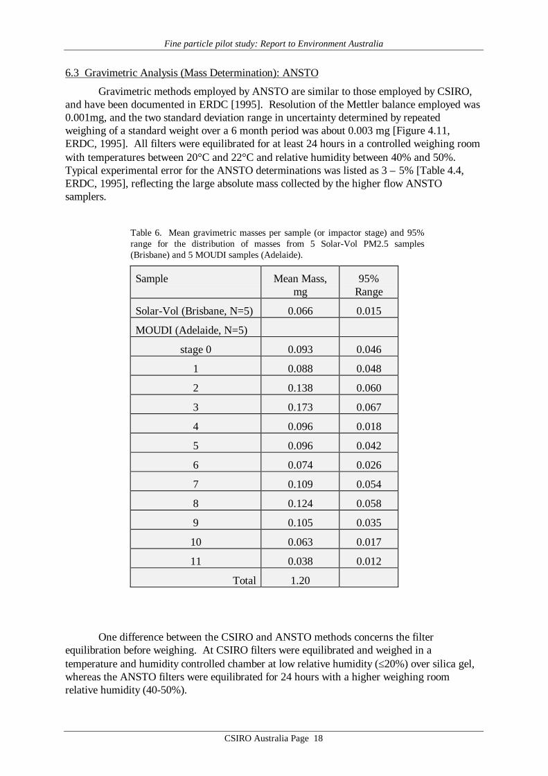
Gravimetric methods employed by ANSTO are similar to those employed by CSIRO,and have been documented in ERDC [1995]. Resolution of the Mettler balance employed was0.001mg, and the two standard deviation range in uncertainty determined by repeatedweighing of a standard weight over a 6 month period was about 0.003 mg [Figure 4.11,ERDC, 1995]. All filters were equilibrated for at least 24 hours in a controlled weighing roomwith temperatures between 20°C and 22°C and relative humidity between 40% and 50%.Typical experimental error for the ANSTO determinations was listed as 3 – 5% [Table 4.4,ERDC, 1995], reflecting the large absolute mass collected by the higher flow ANSTOsamplers.
Table 6. Mean gravimetric masses per sample (or impactor stage) and 95%range for the distribution of masses from 5 Solar-Vol PM2.5 samples(Brisbane) and 5 MOUDI samples (Adelaide).
Sample Mean Mass,mg
95%Range
Solar-Vol (Brisbane, N=5) 0.066 0.015
MOUDI (Adelaide, N=5)
stage 0 0.093 0.046
1 0.088 0.048
2 0.138 0.060
3 0.173 0.067
4 0.096 0.018
5 0.096 0.042
6 0.074 0.026
7 0.109 0.054
8 0.124 0.058
9 0.105 0.035
10 0.063 0.017
11 0.038 0.012
Total 1.20
One difference between the CSIRO and ANSTO methods concerns the filterequilibration before weighing. At CSIRO filters were equilibrated and weighed in atemperature and humidity controlled chamber at low relative humidity (≤20%) over silica gel,whereas the ANSTO filters were equilibrated for 24 hours with a higher weighing roomrelative humidity (40-50%).
Fine particle pilot study: Report to Environment Australia
CSIRO Australia Page 19
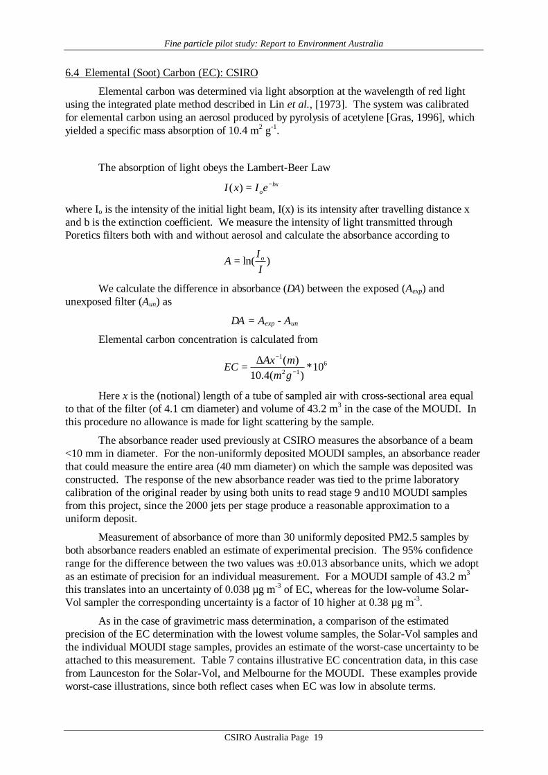
6.4 Elemental (Soot) Carbon (EC): CSIRO
Elemental carbon was determined via light absorption at the wavelength of red lightusing the integrated plate method described in Lin et al., [1973]. The system was calibratedfor elemental carbon using an aerosol produced by pyrolysis of acetylene [Gras, 1996], whichyielded a specific mass absorption of 10.4 m2 g-1.
The absorption of light obeys the Lambert-Beer Lawbx
oeIxI −=)(
where Io is the intensity of the initial light beam, I(x) is its intensity after travelling distance xand b is the extinction coefficient. We measure the intensity of light transmitted throughPoretics filters both with and without aerosol and calculate the absorbance according to
)ln(II
A o=
We calculate the difference in absorbance (∆A) between the exposed (Aexp) andunexposed filter (Aun) as
∆A = Aexp - Aun
Elemental carbon concentration is calculated from
612
1
10*)(4.10
)(−
−∆=gmmAxEC
Here x is the (notional) length of a tube of sampled air with cross-sectional area equalto that of the filter (of 4.1 cm diameter) and volume of 43.2 m3 in the case of the MOUDI. Inthis procedure no allowance is made for light scattering by the sample.
The absorbance reader used previously at CSIRO measures the absorbance of a beam<10 mm in diameter. For the non-uniformly deposited MOUDI samples, an absorbance readerthat could measure the entire area (40 mm diameter) on which the sample was deposited wasconstructed. The response of the new absorbance reader was tied to the prime laboratorycalibration of the original reader by using both units to read stage 9 and10 MOUDI samplesfrom this project, since the 2000 jets per stage produce a reasonable approximation to auniform deposit.
Measurement of absorbance of more than 30 uniformly deposited PM2.5 samples byboth absorbance readers enabled an estimate of experimental precision. The 95% confidencerange for the difference between the two values was ±0.013 absorbance units, which we adoptas an estimate of precision for an individual measurement. For a MOUDI sample of 43.2 m3
this translates into an uncertainty of 0.038 µg m-3 of EC, whereas for the low-volume Solar-Vol sampler the corresponding uncertainty is a factor of 10 higher at 0.38 µg m-3.
As in the case of gravimetric mass determination, a comparison of the estimatedprecision of the EC determination with the lowest volume samples, the Solar-Vol samples andthe individual MOUDI stage samples, provides an estimate of the worst-case uncertainty to beattached to this measurement. Table 7 contains illustrative EC concentration data, in this casefrom Launceston for the Solar-Vol, and Melbourne for the MOUDI. These examples provideworst-case illustrations, since both reflect cases when EC was low in absolute terms.

Fine particle pilot study: Report to Environment Australia
CSIRO Australia Page 20
For the Solar-Vol the data combination of the mean loading of 3.4 µg m-3 with anuncertainty of 0.38 µg m-3 implies an uncertainty of about ±11%. For the MOUDI, it is clearthat some of the individual stages returned EC values close to zero and would showindividually a large relative uncertainty. The total EC value produced by summing all 12stages was low in the Melbourne samples, at 1.90 µg m-3. Accumulating an uncertainty of±0.038 µg m-3 per stage over 12 stages yields overall a figure of ±0.46 µg m-3, or a fractionaluncertainty for the Melbourne samples of ±24%.
Table 7. Mean EC concentration per sample (or impactor state) and 95%range for the distribution of EC concentrations from 5 Solar-Vol PM2.5samples (Launceston) and 5 MOUDI samples (Melbourne).
Sample EC , µg m-3 95% RangeSolar-Vol (Launceston, N=5) 3.4 1.2MOUDI (Melbourne, N=5)
stage 0 0.083 0.1031 0.080 0.1102 0.081 0.0963 0.090 0.1104 0.111 0.1135 0.169 0.1416 0.171 0.1397 0.278 0.1018 0.256 0.1529 0.165 0.14510 0.248 0.14311 0.171 0.130
Total 1.90
6.5 Elemental (Soot) Carbon (EC): ANSTO
Elemental carbon was determined by ANSTO using the Laser Integrated Plate Method(LIPM), a variation of the light absorption method. The application of this method byANSTO has been documented in detail in ERDC [1995], with typical experimental errorslisted as 4-9%, depending on mass loading [see Table 4.4, ERDC, 1995]. The LIPMtechnique has been calibrated at ANSTO for PM2.5 elemental carbon using an aerosolproduced by the burning of a common candle. The system was found to be very linear overlarge absorption ranges corresponding to 0< ln[I0/I] <6 with corresponding elemental carbonloading up to 100 µg cm-2 . A specific mass absorption of (10.4±0.9) m2 g-1 was obtainedwhich was identical to that obtained by CSIRO.
A number of differences exist between the CSIRO and ANSTO determinations of ECby optical absorption methods: (1) the CSIRO absorbance readers employed lower intensitymonochromatic LED light sources, whereas the ANSTO instrument employs a HeNe laserlight source (633nm); (2) the CSIRO filter substrates were polycarbonate sheet filters (Poretics– a “surface” collection medium) while the ANSTO filter substrates were stretched teflon

Fine particle pilot study: Report to Environment Australia
CSIRO Australia Page 21
(Gelman- a “depth” collection medium), and (3) the ANSTO method employed a scale factorto correct for “layering” of the aerosol on the filter, with the factor averaging ~2 [see Section4.1.5 in ERDC, 1995]. In a review of methods used to measure EC, Heintzenberg et al.,[1997] discuss the advantages and disadvantages of these different measurement methods.Surface collection filters are thought to produce a simpler sample/substrate optical geometrythat results in less interaction of scattered light between the particles and the filter medium.
6.6 PIXE (Proton Induced X-ray Emission) Analyses
Nuclear methods, primarily the PIXE techniques, were used to analyse the elements H,F, Na, Al, Si, P, S, Cl, K, Ca, Ti, V, Cr, Mn, Fe, Cu, Co, Ni, Zn, Br, Pb. These measurementswere carried out by the Nuclear Science Applications group at ANSTO. Typical minimumdetection limits (mdl) for each species measured on a MOUDI filters (i.e. the worst case interms of loading per filter) are listed in Table 8. Minimum detection limits for the PIXEmethod on teflon and Nuclepore filters are significantly lower (better) than those given inTable 8.
Table 8. Typical minimum detection limitsfor elements analysed by PIXE in µg m-3 onMOUDI filters assuming a sample volume of43.2 m3.
Element minimum detection limitF 0.0192
Na 0.0769Al 0.0096Si 0.0050P 0.0046Si 0.0038Cl 0.0038K 0.0027Ca 0.0023Ti 0.0019V 0.0015Cr 0.0015Mn 0.0012Fe 0.0008Cu 0.0008Co 0.0008Ni 0.0008Zn 0.0008Br 0.0012Pb 0.0031
The PIXE techniques involve bombarding samples within an evacuated chamber with2.6 MeV protons. An 8 mm diameter beam is used to maintain the integrity of the filters;teflon filters which are more prone to damage are hit with an incident proton charge of 3 µC,while the Nuclepore MOUDI filters, because of the small amount of material on these filters,

Fine particle pilot study: Report to Environment Australia
CSIRO Australia Page 22
were hit with an incident proton charge of 30 µC. An example of a typical PIXE spectrumfrom a Teflon filter is shown in Figure 2.
It is important to note that a few of the elements analysed in some MOUDI sampleswere well below the mdl for those elements, particularly on some finer stage filters as thesample was spread across the twelve separate stages. However the major aerosol parameters,gravimetric mass, EC and total ionic mass, and commonly occurring elements such as S, Cl, K,Fe, Zn, Br and Pb, were above the detection limits.
PM2.5 Teflon Filter -Adelaide-20 August 1997
1
10
100
1000
10000
0 5 10 15
X-ray Energy keV
Coun
ts p
er 3
µC
Raw Spectrum
Background
Fitted SpectrumSi
S Cl
K
Mn
Fe
CuZn
Pb Br
Figure 2. A Typical PIXE spectrum for an exposed Teflon filter obtained in afew minutes of exposure to 2.6 MeV protons.
6.7 Ion Chromatography (IC) Analyses
Suppressed ion chromatography (IC) was used to determine the concentration ofsoluble ions Na+, NH4
+, K+, Mg2+, Ca2+, Cl-, NO3-, SO4
2-, Br-, NO2-, PO4
3-, F-, acetate, formate,oxalate and methanesulfonic acid (MSA). IC was carried out within the Acidity and AerosolsGroup of the CSIRO Division of Atmospheric Research. Filters were extracted in 12 ml ofMilli-Q HPLC grade (high purity de-ionised) water. The hydrophobic Teflon filters werewetted with 100 µl AR grade methanol before extraction to ensure proper aqueous wetting,and a bactericide (120 µl of chloroform) was added to preserve the extracted sample frombiological degradation after extraction.
The ions were determined using a Dionex DX500 gradient ion chromatographemploying Dionex IC columns, an AS11 column and ARS1 suppressor for anions, a CS12column and CRS1 suppressor for the cations. Table 9 shows the detection limits (dl) for eachspecies assuming an air sample volume of 43.2 m3, typical for the MOUDI operating for 24hours. Detection limits for the lowest volume sampler employed, the Solar-Vol PM2.5sampler, are a factor of 10 higher than those given in Table 9.

Fine particle pilot study: Report to Environment Australia
CSIRO Australia Page 23
Table 9. Detection limits for ions analysed by ICassuming sample volume of 43.2 m3 and peakheight 3 times the chromatogram baseline S/N ratio.
Ion Detection Limit (ng m-3)Na+ 0.064NH4
+ 0.053K+ 0.109Mg2+ 0.068Ca2+ 0.111Cl- 0.171NO2
- 0.552Br- 0.377NO3
- 0.293SO4
2- 0.213Oxalate 0.264Acetate 0.285Formate 0.268F- 0.472MSA 0.221
One of the routine quality assurance components employed in the IC laboratory is aprogram of “blind” duplicate analyses. A few percent of samples, randomly selected, aresubjected to "blind" duplicate analyses as a means of objectively determining analyticalprecision on the actual samples under study. Table 10 lists average and median % fractionaldifference between duplicates for selected ions, together with the average aqueous ionconcentration across one set of duplicates.
Table 10. Mean ion concentrations, average % differences and median % differences derived from 15pairs of “blind’ duplicate analyses carried out on randomly selected samples.
Mean conc. µmol l-1 Average % deviation Median % deviationNa+ 48.3 4.8 1.4K+ 3.7 10.1 3.4Mg2+ 7.2 6.5 2.5Ca2+ 5.7 4.3 1.0NH4
+ 90.0 3.7 1.1Cl- 59.7 5.9 3.7NO3
- 16.1 5.1 3.9SO4
2- 18.8 4.4 3.4PO4
3- 5.6 4.1 4.5C2O4
2- 2.4 6.2 4.2HCOOH 15.2 6.3 2.8CH3COOH 9.5 6.7 4.5
Fine particle pilot study: Report to Environment Australia
CSIRO Australia Page 24
6.8 pH Determination
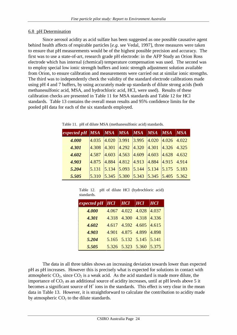
Since aerosol acidity as acid sulfate has been suggested as one possible causative agentbehind health affects of respirable particles [e.g. see Vedal, 1997], three measures were takento ensure that pH measurements would be of the highest possible precision and accuracy. Thefirst was to use a state-of-art, research grade pH electrode: in the AFP Study an Orion Rosselectrode which has internal (chemical) temperature compensation was used. The second wasto employ special low ionic strength buffers and ionic strength adjustment solution availablefrom Orion, to ensure calibration and measurements were carried out at similar ionic strengths.The third was to independently check the validity of the standard electrode calibrations madeusing pH 4 and 7 buffers, by using accurately made up standards of dilute strong acids (bothmethanesulfonic acid, MSA, and hydrochloric acid, HCl, were used). Results of thesecalibration checks are presented in Table 11 for MSA standards and Table 12 for HClstandards. Table 13 contains the overall mean results and 95% confidence limits for thepooled pH data for each of the six standards employed.
Table 11. pH of dilute MSA (methanesulfonic acid) standards.
expected pH MSA MSA MSA MSA MSA MSA MSA
4.000 4.035 4.020 3.991 3.995 4.020 4.026 4.0224.301 4.308 4.301 4.292 4.320 4.301 4.326 4.3254.602 4.587 4.603 4.563 4.609 4.603 4.628 4.6324.903 4.875 4.884 4.812 4.913 4.884 4.915 4.9145.204 5.131 5.134 5.093 5.144 5.134 5.175 5.1835.505 5.310 5.345 5.300 5.343 5.345 5.405 5.362
Table 12. pH of dilute HCl (hydrochloric acid)standards.
expected pH HCl HCl HCl HCl
4.000 4.067 4.022 4.028 4.0374.301 4.318 4.300 4.318 4.3364.602 4.617 4.592 4.605 4.6154.903 4.901 4.875 4.899 4.8985.204 5.165 5.132 5.145 5.1415.505 5.326 5.323 5.360 5.375
The data in all three tables shows an increasing deviation towards lower than expectedpH as pH increases. However this is precisely what is expected for solutions in contact withatmospheric CO2, since CO2 is a weak acid. As the acid standard is made more dilute, theimportance of CO2 as an additional source of acidity increases, until at pH levels above 5 itbecomes a significant source of H+ ions in the standards. This effect is very clear in the meandata in Table 13. However, it is straightforward to calculate the contribution to acidity madeby atmospheric CO2 to the dilute standards.

Fine particle pilot study: Report to Environment Australia
CSIRO Australia Page 25
Table 13. Mean pH and 95%confidence limits for dilute acidstandards.
expected pH mean 95%c.l.
4.000 4.022 0.041
4.301 4.312 0.027
4.602 4.605 0.037
4.903 4.889 0.056
5.204 5.148 0.059
5.505 5.358 0.109
In Figure 3 the mean calibration data from Table 13 are plotted with a theoretical pHcurve produced by adding to the dilute acid standard the additional CO2-derived aciditycalculated from the known solubility and acidity constants for CO2, and an assumedatmospheric mixing ratio of 370 ppm in the laboratory air. Clearly the deviation from the 1:1line may be ascribed quantitatively to the effects of atmospheric CO2, and the performance ofthe pH measurement system in the AFP Study can be rated as excellent.
4.0
4.2
4.4
4.6
4.8
5.0
5.2
5.4
5.6
5.8
6.0
4.0 4.2 4.4 4.6 4.8 5.0 5.2 5.4 5.6 5.8 6.0
standard (no CO2) pH
mea
sure
d an
d ca
lcul
ated
pH
(with
CO
2)
Calculated (with CO2)Dilute acid standards
Figure 3. Mean values from laboratory from pH calibration checks, based on dilute strongacid standard solutions (Table 13). The dashed line depicts unity slope. The calculatedcurve shows the expected pH assuming equilibrium between the standards andatmospheric CO2.
Fine particle pilot study: Report to Environment Australia
CSIRO Australia Page 26
6.9 MOUDI Data Analysis
6.9.1 Blank Subtractions
PIXE and IC analyses were performed on unexposed new Poretics, Nuclepore andFluoropore filters with each batch of analyses. For IC, concentrations determined from theblank filter were always below the IC detection limit. As some of the species determined onthe MOUDI samples by PIXE were below the PIXE minimum detection limit it was necessaryto subtract the blank filter measurements made with each batch from the PIXE results.
6.9.2 Scaling PIXE data
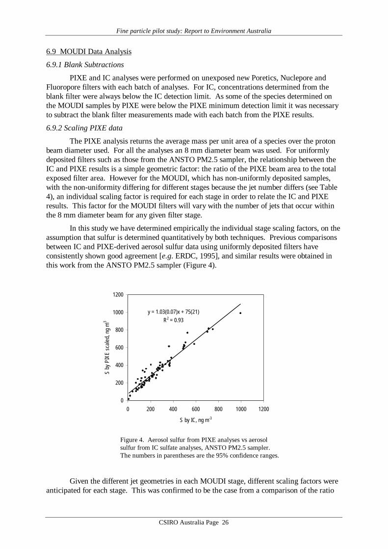
The PIXE analysis returns the average mass per unit area of a species over the protonbeam diameter used. For all the analyses an 8 mm diameter beam was used. For uniformlydeposited filters such as those from the ANSTO PM2.5 sampler, the relationship between theIC and PIXE results is a simple geometric factor: the ratio of the PIXE beam area to the totalexposed filter area. However for the MOUDI, which has non-uniformly deposited samples,with the non-uniformity differing for different stages because the jet number differs (see Table4), an individual scaling factor is required for each stage in order to relate the IC and PIXEresults. This factor for the MOUDI filters will vary with the number of jets that occur withinthe 8 mm diameter beam for any given filter stage.
In this study we have determined empirically the individual stage scaling factors, on theassumption that sulfur is determined quantitatively by both techniques. Previous comparisonsbetween IC and PIXE-derived aerosol sulfur data using uniformly deposited filters haveconsistently shown good agreement [e.g. ERDC, 1995], and similar results were obtained inthis work from the ANSTO PM2.5 sampler (Figure 4).
y = 1.03(0.07)x + 75(21)R2 = 0.93
0
200
400
600
800
1000
1200
0 200 400 600 800 1000 1200
S by IC, ng m-3
S by
PIX
E sc
aled
, ng
m-3
Figure 4. Aerosol sulfur from PIXE analyses vs aerosolsulfur from IC sulfate analyses, ANSTO PM2.5 sampler.The numbers in parentheses are the 95% confidence ranges.
Given the different jet geometries in each MOUDI stage, different scaling factors wereanticipated for each stage. This was confirmed to be the case from a comparison of the ratio
Fine particle pilot study: Report to Environment Australia
CSIRO Australia Page 27
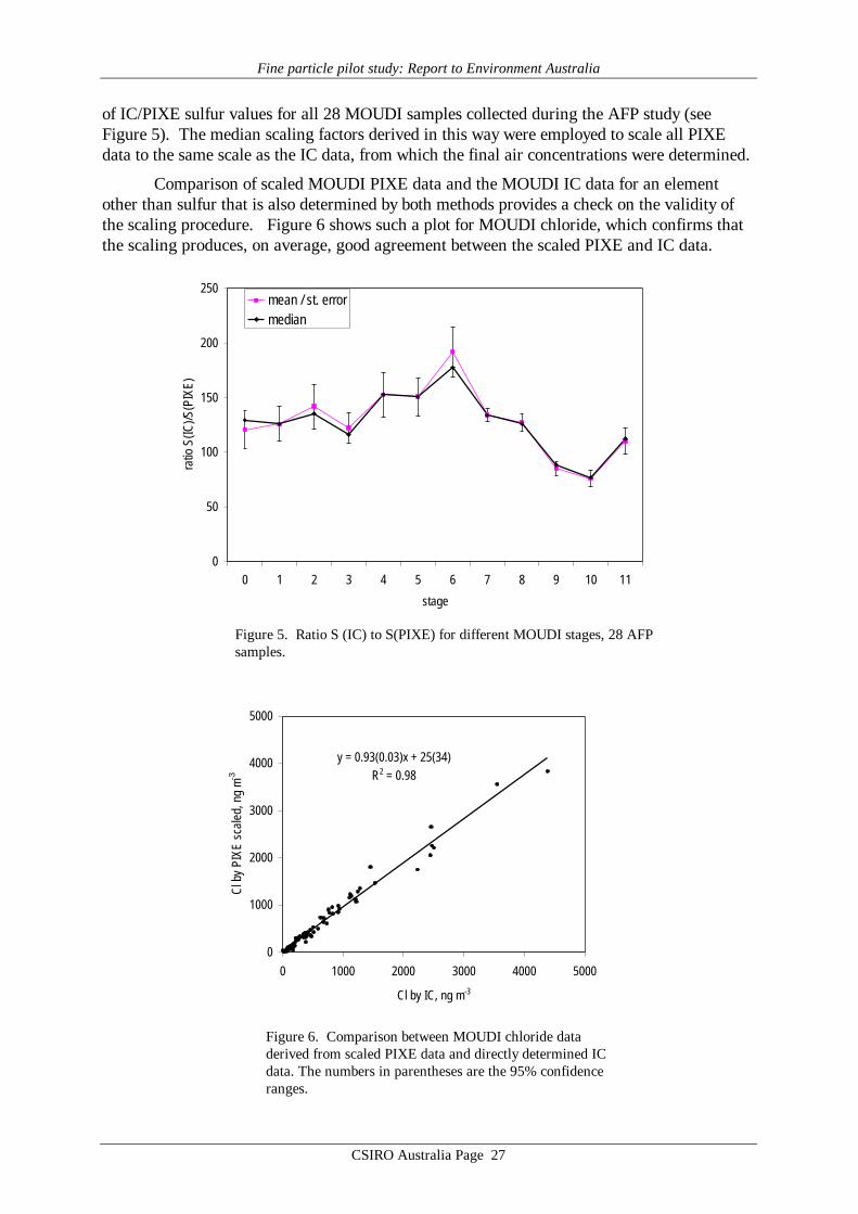
of IC/PIXE sulfur values for all 28 MOUDI samples collected during the AFP study (seeFigure 5). The median scaling factors derived in this way were employed to scale all PIXEdata to the same scale as the IC data, from which the final air concentrations were determined.
Comparison of scaled MOUDI PIXE data and the MOUDI IC data for an elementother than sulfur that is also determined by both methods provides a check on the validity ofthe scaling procedure. Figure 6 shows such a plot for MOUDI chloride, which confirms thatthe scaling produces, on average, good agreement between the scaled PIXE and IC data.
0
50
100
150
200
250
0 1 2 3 4 5 6 7 8 9 10 11
stage
ratio
S(IC
)/S(P
IXE)
mean / st. errormedian
Figure 5. Ratio S (IC) to S(PIXE) for different MOUDI stages, 28 AFPsamples.
y = 0.93(0.03)x + 25(34)R2 = 0.98
0
1000
2000
3000
4000
5000
0 1000 2000 3000 4000 5000
Cl by IC, ng m-3
Cl b
y PI
XE s
cale
d, n
g m-3
Figure 6. Comparison between MOUDI chloride dataderived from scaled PIXE data and directly determined ICdata. The numbers in parentheses are the 95% confidenceranges.

Fine particle pilot study: Report to Environment Australia
CSIRO Australia Page 28
6.9.3 Data Inversion
The MOUDI collects the ambient aerosol in 12 discrete, size-fractionated samples soas to provide information on the distribution of chemical components as a function of particlesize. While useful information may be gained simply by plotting the MOUDI data in histogramform, a considerably more powerful result can be achieved by utilising the known size-dependence of each collection stage with a numerical inversion procedure to yield a smoothaerosol mass distribution [Winklmayr et al.,1990].
The MOUDI inversion routine developed by CSIRO was based on the efficient, non-linear iterative inversion procedure of Twomey and Zalabsky [1981], with the MOUDI stagetransmission kernels derived from the Manufacturer’s calibration supplied with the CSIROMOUDI. The individual stage calibration curves were digitised by CSIRO, and fitted withWinklmayr functions [Winklmayr et al.,1990], to yield the suite of kernels shown graphicallyin Figure 7. Smooth distributions of both the stage kernels and MOUDI mass distributionswere obtained by carrying out the calculations using 20 points per decade in logarithmicparticle diameter, over the particle diameter range 0.01 to 100 µm.
Note that a “fictitious” stage function was generated to represent the MOUDI backupfilter (stage 11), having the same shape as the function for stage 10, but a 50% cut-size halfthat of stage 10.
0%
20%
40%
60%
80%
100%
0.01 0.1 1 10 100
Aerodynamic diameter, µm
Tran
smiss
ion
effic
ienc
y
stage 0stage 11
Figure 7. MOUDI kernel functions for each stage.
The inversion procedure convolves an initial “guess” (mass-size) distributionsequentially with each of the stage kernels, compares the resultant calculated stage mass withthe measured stage mass, and adjusts the input “guess” distribution to make the calculated andmeasured stage masses agree. The stage kernel function was used in each case as the

Fine particle pilot study: Report to Environment Australia
CSIRO Australia Page 29
adjustment function, so the overall effect of the procedure was to construct a smooth inputdistribution from a linear combination of the kernel functions shown in Figure 7. The inversionwas constrained to conserve total mass.
The procedure was terminated when either of two conditions was met: (1) theprocedure converged, defined by the change in root-mean-square (rms) residual between fittedand observed stage masses changing by less than 1% between successive iterations, or (2)condition (1) was not met but 10 iterations were reached. In the vast majority of cases theinversion converged in < 6 iterations, with rms residuals of less than 3%. A few inversionswere not accepted: those that did not meet the convergence criterion with 10 iterations, andthose that did meet the convergence criterion but had rms residuals of 4% or greater.
The robustness of the inversion procedure was tested by carrying out numericalexperiments based on typical measured mass distributions from each of the sites. Theexperiments involved carrying out 25 inversions with random error introduced numerically tothe measured stage mass data used as input. Four sets of experiments were carried out,reflecting random error distributions (at 95% confidence) of ±5%, ±10%, ±20% and ±25%applied to the input data. The means of the 25 inverted distributions with added random errorwere in each case found to reproduce almost precisely the original inverted distribution,indicating the absence of any systematic error in the mean response introduced by theincreasing uncertainty added to the input data. Figure 8 shows results from three of thenumerical experiments, where the initial “no added error” distribution is plotted along with themean from the 25 inversions with randomly added error, and the 95% confidence rangederived from the range in the 25 inverted results with added error.
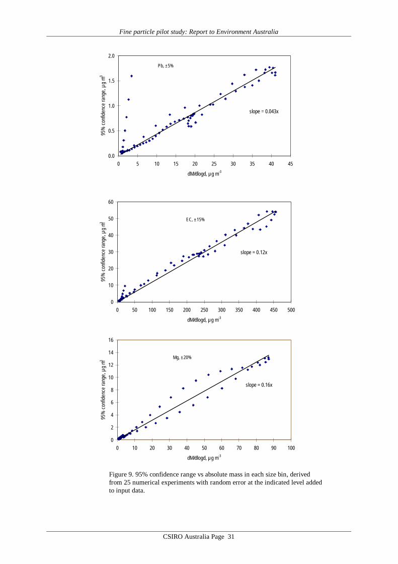
Plots of the 95% confidence ranges against the mass at each diameter are shown inFigure 9. For almost all of the points it is apparent that the output uncertainty scales linearlywith the added input uncertainty, i.e. a random input uncertainty of x% results in a 95% rangein output of about x%, as shown by the slopes of 0.043 (for 5% random error), 0.12 (for 15%random error) and 0.16 (for 20% random error) in Figure 9.
However, each of the plots in Figure 9 also shows a series of ~7 points near the originwhere the fractional output uncertainty error is much larger than the input fractionaluncertainty. These points correspond to the lowest 7 size bins (diameters <0.02 µm). It is notsurprising that the fractional error increases substantially towards the ends of the inverteddistribution, as the inversion procedure effectively has no capability to adjust the sizedistribution at particle sizes beyond those in which the kernels have significant curvature (notethat the kernel for stage 11 is “fictitious” at sizes below ~0.03 µm). Therefore, in allsubsequent inversions the procedure was truncated at a lower size cut-off of 0.05 µm, toconfine the inversion to the diameter range between 0.05 and 30 µm over which sizedependent information is contained in the stage collection characteristics.

Fine particle pilot study: Report to Environment Australia
CSIRO Australia Page 30
0
100
200
300
400
500
600
0.01 0.1 1 10 100
diameter, µm
dM/d
logd
, µg
m-3
Silicon, ±5%
0
100
200
300
400
500
600
0.01 0.1 1 10 100
diameter, µm
dM/d
logd
, µg
m-3
EC, ±10%
0
200
400
600
800
1000
1200
1400
1600
0.01 0.1 1 10 100
diameter, µm
dM/d
logd
, µg
m-3
nssSO4, ±20%
Figure 8. Initial MOUDI distribution (line) and mean distribution plus 95%confidence range derived from 25 numerical experiments with random errorat the indicated level added to input data.
Fine particle pilot study: Report to Environment Australia
CSIRO Australia Page 31
slope = 0.043x
0.0
0.5
1.0
1.5
2.0
0 5 10 15 20 25 30 35 40 45
dM/dlogd, µg m-3
95%
con
fiden
ce ra
nge,
µg
m-3
Pb, ±5%
slope = 0.12x
0
10
20
30
40
50
60
0 50 100 150 200 250 300 350 400 450 500
dM/dlogd, µg m-3
95%
con
fiden
ce ra
nge,
µg
m-3
EC, ±15%
slope = 0.16x
0
2
4
6
8
10
12
14
16
0 10 20 30 40 50 60 70 80 90 100
dM/dlogd, µg m-3
95%
con
fiden
ce ra
nge,
µg
m-3
Mg, ±20%
Figure 9. 95% confidence range vs absolute mass in each size bin, derivedfrom 25 numerical experiments with random error at the indicated level addedto input data.

Fine particle pilot study: Report to Environment Australia
CSIRO Australia Page 32
6.9.4 Interstage losses
The transmission characteristic of the MOUDI include small, size-dependent particlelosses during sample flow path through the device, that were taken into account to remove anyresultant small systematic bias in the MOUDI data. Marple et al. [1991] measured theinterstage losses in the MOUDI for both solid and liquid particles. Their data were fitted tosmooth functions, which are shown in Figure 10. Maximum loss occurs at ~10 µm and at lessthan 0.1 µm, with quite small losses between 0.1 and about 5 µm.
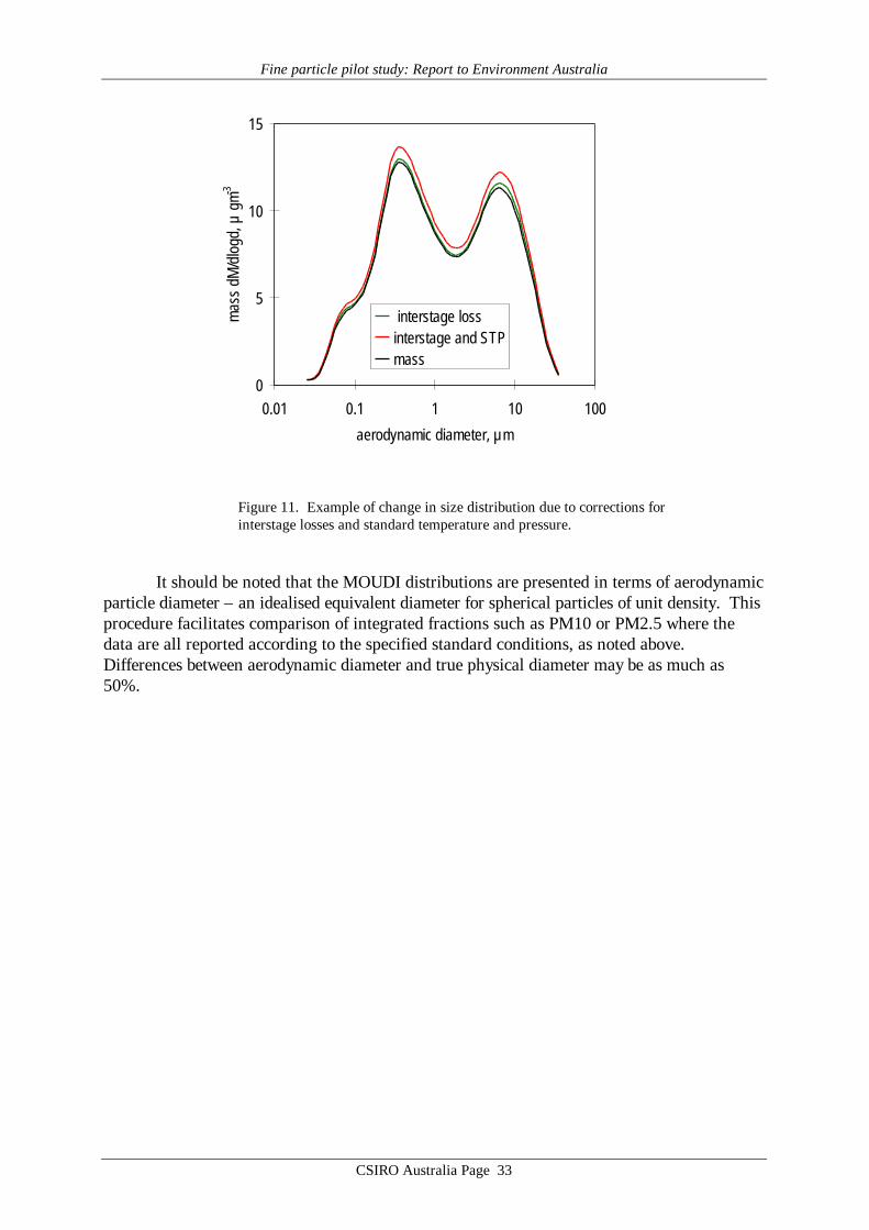
All MOUDI distributions discussed in this work were corrected for interstage lossesusing the average of the curves in Figure 10, on the assumption that at ambient humiditiesencountered in this work at least the subset of particles containing soluble material would bedeliquesced. Any error introduced by simply averaging the two curves is insignificant, as theoverall effect of the interstage loss correction is itself only very minor, as shown in Figure 11.
0%
20%
40%
60%
80%
100%
0.01 0.1 1 10 100
aerodynamic particle diameter, µm
Par
ticle
loss
solid particlesliquid particles
INLET12345678910
STAGE NUMBER
Particle cut-points
Figure 10. Interstage loss function for the MOUDI (Marple et al., 1991).
6.9.5 Standard Temperature and Pressure.
Australian air quality data are reported at conditions of standard temperature andpressure, 273.15 K and 101.3 hPa. The MOUDI flow data were recorded at ambienttemperature and pressure, so require correction to achieve consistency with the other samplingdevices used in the study. These corrections were carried out for each sample using the 24hour mean ambient temperatures and pressures recorded at each site. The importance ofaccounting for the systematic difference between ambient conditions and STP is clearly evidentin Figure 11, which contrasts the magnitude of this correction with the considerably smallercorrection required to account for interstage losses.
Fine particle pilot study: Report to Environment Australia
CSIRO Australia Page 33
0
5
10
15
0.01 0.1 1 10 100
aerodynamic diameter, µm
mas
s dM
/dlo
gd, µ
gm-3
interstage lossinterstage and STPmass
Figure 11. Example of change in size distribution due to corrections forinterstage losses and standard temperature and pressure.
It should be noted that the MOUDI distributions are presented in terms of aerodynamicparticle diameter – an idealised equivalent diameter for spherical particles of unit density. Thisprocedure facilitates comparison of integrated fractions such as PM10 or PM2.5 where thedata are all reported according to the specified standard conditions, as noted above.Differences between aerodynamic diameter and true physical diameter may be as much as50%.

Fine particle pilot study: Report to Environment Australia
CSIRO Australia Page 34
7. Results
In this chapter an overview of the aerosol data collected during the study is tabulatedby site, in chronological order. The purpose of this overview is to provide a broad-scalepicture of the average aerosol properties determined at each site, to set an overall perspectivefrom within which, in subsequent chapters, detailed properties of the aerosol on individualdays will be discussed, along with comparisons between different instruments.
It is important to note that to generate the overview in this chapter we have takensimple averages over all available data from each measurement system at each site. In manyinstances the number of samples averaged differs between instruments, as does the number ofdays on which different systems operated, these disparities arising from a variety of instrumentmalfunctions or other local operational constraints. Thus while the average data in this chapterdo provide a valid perspective on broad-scale aerosol properties, these somewhat disparate (interms of sample numbers per instrument) averages should not be used to draw inferencesconcerning relative instrument performance. The important issue of relative instrumentperformance is specifically addressed in a subsequent chapter using only concurrent data.
7.1 Overview of Aerosol Data by Site
Average values of gravimetric aerosol mass concentration (GM), inorganic massconcentration (IM5), estimated organic matter concentration (EOM6), elemental carbon (EC)mass concentration and elemental/ionic components are presented in Table 14 – 19. Meandata on aerosol mass determined by the CSIRO TEOM, aerosol scattering coefficientdetermined by the CSIRO nephelometer, and ultrafine particle concentration from the CSIROCN counter at each site are presented in Table 20. Note that these latter three data records donot cover all sites or all days at a given site. It should also be noted that the definition of EOMused here assumes total mass closure, that is, that all the gravimetric mass is accounted for bythe organic matter plus EC and the mass associated with the 24 chemical species listed in thedefinition of IM given by Brook et al. [1997]. It specifically does not include water whichmaybe 8 to 10% of the total mass [ERDC 1995] if the filters are not totally dried before hand.Other definitions of EOM which do not assume total mass closure may be used where the totalhydrogen and sulfur content of the filters has been determined [Malm et al., 1994; ERDC1995]. These methods have the advantage that they do not rely on the measurement of somany different chemical species some of which only occur in trace quantities and consequentlyhave a lower standard deviation associated with them. For example, in Table 14, for theANSTO PM2.5 sampler the EOM = 2.9±12.2 µg m-3 by the Brook method applied here and3.6±3.1 µg m-3 by the Malm method. However EOM is calculated and discussed later in thisreport primarily as a check on the consistency of the GM, EC and IM data, not for the purposeof analysing properties of the organic matter content in the aerosol.
One further point to note is that the H measurements for PM2.5 ANSTO samplerslisted in Tables 14 - 19 are for total hydrogen, including hydrogen in organic matter,
5Inorganic Mass is calculated as follows [after Brook et al, 1997]:
IM=H++Na++1.41K++NH4++1.63Ca2++Mg2++Cl-+NO3
-+NO2-+SO4
2-+PO43-
+Pb+Br+1.79V+2.2Al+1.24Zn+2.5Si+1.58Fe+1.94Ti+Cr+Mn+Co+Ni+Cu
6Estimated Organic Matter (EOM) is estimated as follows: EOM=GM-IM-EC

Fine particle pilot study: Report to Environment Australia
CSIRO Australia Page 35
ammonium ions, hydrogen ions and water. The H+ ions quoted with the IC results representthe soluble hydrogen ion concentrations (free acidity) only and hence are not directlycomparable with the H total values.
Reference to the PM10 averages in Tables 14 – 19 obtained from the MOUDI suggeststhat the six sets of results fall into two distinct groupings. The four major cities, Sydney,Brisbane, Melbourne and Adelaide yielded average MOUDI PM10 concentrations in the range20 – 25 µg m-3, whereas Canberra and Launceston yielded averages 2 – 3 times higher at 43and 63 µg m-3. Similar systematic differences are evident in the average IM (inorganic mass)concentrations, which for the four major cities accounts for 30 – 50% of the PM10 loading,but only about 20% for Canberra and Launceston. In the case of EC (elemental carbon)loading the major cities such as Sydney and Adelaide have EC providing ≥10% of PM10,while for Canberra and Launceston the contribution is less than 10%. Finally, the importanceof EOM (estimated organic matter) is systematically higher in the case of Canberra andLaunceston, at about 75% of PM10, whereas in the major cities the contribution to PM10made by EOM is less, down to only about 40% in the Brisbane data.
The means of the physical measurements shown in Table 20 also suggest this pattern ofaerosol loading in the 6 cities, with Canberra and Launceston displaying the highest TEOMPM2.5 concentrations and scattering coefficients.
These absolute values and systematic differences in average aerosol properties sitwithin previous results from various Australian locations such as the Latrobe Valley,Melbourne, Sydney, Perth, Launceston and Brisbane [Ayers et al., 1990; Gras et al. 1992;ERDC, 1995; Gras, 1996; Working Party, 1996; Chan et al., 1997], and point towards thedifferent aerosol sources already identified for the regions in question.
The major difference evident in the AFP data is that in Canberra and Launceston, thewinter-time aerosol is dominated by emissions from domestic wood-burning (relatively highPM loadings; EOM; nssK+; with relatively low EC), while in the major cities the wintertimeaerosol, while having some wood smoke component, has a greater fractional contribution fromautomotive emissions.
It is notable that the PM10 loadings of all samples from the four major cities fall belowthe proposed national standard of 50 µg m-3, 24 hour average, while both Canberra andLaunceston have individual samples greater than this value. More notable is the Launcestondata, with the average of the five 24h means, at 63 µg m-3, being well above the proposed 24hour figure.

Fine particle pilot study: Report to Environment Australia
CSIRO Australia Page 36
Table 14. Means ±stdev Sydney August 1996ANSTO SAMPLERS MOUDI
MASSES µg cm-3 PM10 PM2.5 PM10 PM2.5mass 18.3 ± 11.6 9.6 ± 7.1 24.7 ± 9.6 18.5 ± 14.3IM 6.1 ± 2.9 2.2 ± 1.3 7.5 ± 2.4 5.1 ± 3.8EC 3.7 ± 3.3 4.4 ± 3.8 2.4 ± 1.0 2.1 ± 1.7EOM 8.5 ± 17.9 2.9 ± 12.2 14.8 ± 13.1 11.2 ± 19.8
ANSTO SAMPLERS MOUDIPIXE ng m-3 PM10 PM2.5 PM10 PM2.5H7 409 ± 324Na 1366 ± 1409 224 ± 383 671 ± 531 196 ± 57Al 215 ± 106 28 ± 21 49 ± 32Si 885 ± 443 62 ± 44 257 ± 161 71 ± 41P 20 ± 12.1 5.2 ± 3.5S 361 ± 266 339 ± 228 324 ± 146 293 ± 139Cl 840 ± 723 295 ± 254 130 ± 158 16 ± 14K 141 ± 86 80 ± 47 113 ± 55 70 ± 48Ca 216 ± 134 30 ± 18 120 ± 124 22 ± 11Ti 37 ± 23.5 3.7 ± 3.1 13 ± 7V 5.4 ± 1.9Cr 4.9 ± 2.0 2.8 ± 0.5 2.0 ± 0.4Mn 13 ± 11 3.0 ± 3.3 5.0 ± 2 3.0 ± 1Fe 350 ± 262 59 ± 53 155 ± 98 61 ± 39Co 4.2 ± 2.1 5.6 ± 2.2 3.6 ± 1.9Ni 4.7 ± 1.7Cu 14.3 ± 5.7 7.1 ± 9.8 30 ± 60 7 ± 10Zn 29 ± 20 25 ± 18 38 ± 33 25 ± 24Br 42 ± 20 31 ± 19 34 ± 16 31 ± 15Pb 95 ± 71 77 ± 48 94 ± 52 85 ± 48
ANSTO SAMPLERS MOUDIIC ng m-3 PM10 PM2.5 PM10 PM2.5H+ 1.8 ± 0.4 1.2 ± 0.9 11 ± 3 9.2 ± 3Na 624 ± 355 217 ± 158 520 ± 321 228 ± 77NH4
+ 95 ± 115 224 ± 248 392 ± 187 380 ± 183K+ 98 ± 59 71 ± 50 133 ± 63 111 ± 61nssK+ 81 ± 55 65 ± 51 115 ± 63 106 ± 60Mg2+ 87 ± 46 28 ± 20 58 ± 40 18 ± 8Ca2+ 165 ± 95 27 ± 10 112 ± 44 54 ± 15Cl- 682 ± 562 311 ± 239 372 ± 384 132 ± 82NO2
- 1.9 ± 0.2 0.9 ± 0.3 16 ± 16 14 ± 17Br- 12 ± 10.9 19 ± 16 11 ± 7 9.7 ± 7NO3
- 395 ± 398 269 ± 278 741 ± 318 356 ± 156SO4
2- 631 ± 516 611 ± 490 971 ± 435 875 ± 421nssSO4
2- 584 ± 503 596 ± 493 852 ± 428 828 ± 418Oxalic acid 44 ± 43 35 ± 38 135 ± 102 109 ± 83PO4
3- 19 ± 20 3.0 ± 2 1.9 ± 1Acetic acid 18 ± 4 6.1 ± 2 119 ± 61 104 ± 61Formic acid 54 ± 10 8.9 ± 2 90 ± 24 70 ± 21MSA 11 ± 5 10.9 ± 6.8 4.0 ± 2.3 3.7 ± 2.3
7 Note that H (total H) determined by PIXE and H+ (soluble H+ ion concentration) determined from pH are notcomparable measurements.

Fine particle pilot study: Report to Environment Australia
CSIRO Australia Page 37
Table 15. Means ±stdev Brisbane September, October, November 1996ANSTO SAMPLERS MOUDI
MASSES µg cm-3 PM10 PM2.5 PM10 PM2.5mass 18.1 ± 5.9 6.0 ± 2.4 20.0 ± 7.8 11.2 ± 7.7IM 8.7 ± 3.5 2.4 ± 0.8 10.8 ± 3.7 5.6 ± 3.7EC 1.6 ± 1.2 1.5 ± 0.8 1.7 ± 0.3 1.6 ± 1.3EOM 7.8 ± 10.5 2.0 ± 4.0 7.5 ± 11.8 4.0 ± 12.7
ANSTO SAMPLERS MOUDIPIXE ng m-3 PM10 PM2.5 PM10 PM2.5H 194 ± 99Na 2176 ± 1143 314 ± 174 2162 ± 935 482 ± 320Al 156 ± 78 23 ± 13Si 732 ± 296 70 ± 30 210 ± 120 60 ± 38P 20 ± 5.1 5.0 ± 3.8S 409 ± 175 326 ± 154 349 ± 202 281 ± 190Cl 1297 ± 1205 321 ± 387 900 ± 973 167 ± 194K 146 ± 75 76 ± 55 199 ± 102 88 ± 80Ca 190 ± 63 32 ± 7 214 ± 87 31 ± 5Ti 38 ± 18.5 6.7 ± 4.8 11 ± 8V 2 ± 1.7Cr 7 ± 1.4Mn 7 ± 4 3 ± 2 5 ± 2 3 2Fe 229 ± 114 48 ± 26 121 ± 94 44 ± 35Co 3.3 ± 1.5 5.3 ± 2.4 3 2Ni 3.5 ± 1.6Cu 9.7 ± 3.8 3.3 ± 2.1 146 ± 62 43 ± 18Zn 29 ± 9 20 ± 11 41 ± 13 24 ± 18Br 22 ± 10 9 ± 6 11 ± 3 8 ± 4Pb 36 ± 26 31 ± 25 27 ± 15 23 ± 13
ANSTO SAMPLERS MOUDIIC ng m-3 PM10 PM2.5 PM10 PM2.5H+ 1.5 ± 0.5 0.6 ± 0.2 9 ± 3 8 ± 3Na 1479 ± 952 419 ± 224 1532 ± 588 554 ± 295NH4
+ 71 ± 96 115 ± 74 373 ± 190 347 ± 191K+ 123 ± 70 68 ± 56 252 ± 157 161 ± 121nssK+ 89 ± 62 58 ± 55 204 ± 146 148 ± 117Mg2+ 180 ± 109 52 ± 26 153 ± 57 41 ± 16Ca2+ 200 ± 61 34 ± 8 186 ± 77 71 ± 33Cl- 1400 ± 1392 303 ± 372 1133 ± 818 318 ± 192NO2
- 8.4 ± 22.1 34 ± 27 27 ± 21Br- 5 ± 3 8 ± 7 6 ± 7NO3
- 1297 ± 1100 242 ± 86 2505 ± 1409 895 ± 682SO4
2- 992 ± 495 745 ± 418 1044 ± 607 838 ± 572nssSO4
2- 896 ± 468 717 ± 416 765 ± 598 744 ± 570Oxalic acid 78 ± 67 62 ± 57 130 ± 113 94 ± 85PO4
3-
Acetic acid 19 ± 3 6 ± 1 211 ± 165 160 ± 120Formic acid 82 ± 30 9 ± 2 134 ± 58 92 ± 35MSA 16 ± 5 16.0 ± 6.1 8.8 ± 8.5 6.8 ± 6.5

Fine particle pilot study: Report to Environment Australia
CSIRO Australia Page 38
Table 16. Means ±stdev Melbourne April 1997ANSTO SAMPLERS MOUDI
MASSES µg cm-3 PM10 PM2.5 PM10 PM2.5mass 17.5 ± 4.2 4.9 ± 2.6 23.5 ± 5.4 14.8 ± 10.6IM 9.5 ± 2.1 2.0 ± 0.2 8.3 ± 2.1 4.2 ± 2.7EC 1.7 ± 0.8 1.6 ± 0.7 1.8 ± 1.3 1.5 ± 1.2EOM 6.4 ± 7.0 1.3 ± 3.5 13.3 ± 8.8 9.1 ± 14.5
ANSTO SAMPLERS MOUDIPIXE ng m-3 PM10 PM2.5 PM10 PM2.5H 203 ± 110Na 2015 ± 645 68 ± 153 1921 ± 777 633 ± 231Al 223 ± 151 41 ± 10 37 ± 14Si 1103 ± 583 136 ± 34 325 ± 126 108 ± 44P 10 ± 12 10 ± 8.9S 348 ± 102 269 ± 97 302 ± 114 231 ± 101Cl 1178 ± 795 97 ± 87 1136 ± 760 218 ± 155K 119 ± 56 50 ± 18 70 ± 28 35 ± 18Ca 317 ± 114 44 ± 8 117 ± 65 25 ± 13Ti 45 ± 24 7.0 ± 4.3 15 ± 6.2 5.0 ± 1.8VCr 4.4 ± 2.5Mn 12 ± 1.7 3.3 ± 2.3 6.6 ± 3.0 3.8 ± 2.8Fe 459 ± 185 75 ± 21 208 ± 50 77 ± 19Co 2.1 ± 1.9 2.6 ± 1.2 1.7 ± 0.7Ni 2.3 ± 1.1 0.6 ± 0.6Cu 5.7 ± 2.8 1.3 ± 0.7Zn 332 ± 298 118 ± 161 208 ± 247 145 ± 181Br 33 ± 18 20 ± 18 22 ± 16 17 ± 14Pb 60 ± 44 51 ± 36 58 ± 45 50 ± 43
ANSTO SAMPLERS MOUDIIC ng m-3 PM10 PM2.5 PM10 PM2.5H+ 0.9 ± 0.6 0.7 ± 0.3 7.2 ± 0.7 5.7 ± 0.6Na 1146 ± 487 173 ± 45 1139 ± 363 381 ± 69NH4
+ 32 ± 24 97 ± 71 196 ± 107 186 ± 107K+ 85 ± 19 44 ± 21 87 ± 28 55 ± 25nssK+ 59 ± 19 41 ± 21 54 ± 22 47 ± 23Mg2+ 136 ± 50 14 ± 3.9 109 ± 46 27 ± 9.2Ca2+ 235 ± 77 35 ± 5.8 153 ± 28 66 ± 18Cl- 1399 ± 934 97 ± 82 1208 ± 549 267 ± 96NO2
- 18 ± 10.1 13 ± 7.5Br- 15 ± 11 8.9 ± 10 16 ± 17 14 ± 16NO3
- 560 ± 355 69 ± 35 889 ± 566 340 ± 160SO4
2- 842 ± 216 558 ± 206 921 ± 333 699 ± 305nssSO4
2- 770 ± 207 550 ± 206 692 ± 282 638 ± 287Oxalic acid 36 ± 18 20 ± 10 37 ± 24 30 ± 24PO4
3- 16 ± 15 14 ± 11Acetic acid 20 ± 6.6 7.1 ± 2.8 94 ± 53 69 ± 42Formic acid 95 ± 27 8.9 ± 2.6 110 ± 12 68 ± 12MSA 15 ± 3.3 14 ± 3.2 6.7 ± 3.1 5.9 ± 2.5

Fine particle pilot study: Report to Environment Australia
CSIRO Australia Page 39
Table 17. Means ±stdev Canberra May 1997ANSTO SAMPLERS MOUDI
MASSES µg cm-3 PM10 PM2.5 PM10 PM2.5mass 16.1 ± 7.8 9.1 ± 6.7 43.1 ± 22.4 34.3 ± 24.6IM 5.1 ± 3.8 1.4 ± 1.6 8.8 ± 1.2 5.8 ± 4.1EC 2.7 ± 1.6 2.3 ± 1.9 3.4 ± 0.6 2.7 ± 2.1EOM 8.3 ± 13.1 5.3 ± 10.2 30.8 ± 24.3 25.8 ± 30.8
ANSTO SAMPLERS MOUDIPIXE ng m-3 PM10 PM2.5 PM10 PM2.5H 412 ± 320Na 1036 ± 475 1016 ± 498 403 ± 113Al 132 ± 127 20 ± 22 41 ± 14Si 688 ± 516 44 ± 53 306 ± 134 88 ± 38P 14.5 ± 6.4 6.8 ± 3.9S 402 ± 361 270 ± 342 464 ± 212 422 ± 204Cl 135 ± 138 55 ± 51 122 ± 82 37 ± 38K 117 ± 91 69 ± 62 180 ± 103 136 ± 110Ca 69 ± 50 14 ± 16 48 ± 28 12 ± 7.2Ti 14 ± 14 1.6 ± 2.1 8.0 ± 2.3V 0.8 ± 0.4 0.1 ± 0.2Cr 4.6 ± 0.2 0.2 ± 0.3Mn 5.5 ± 3.3 0.6 ± 0.9 4.3 ± 1.1 2.0 ± 0.2Fe 133 ± 118 23 ± 27 115 ± 30 41 ± 15Co 3.7 ± 1.9 2.0 ± 0.9Ni 1.3 ± 0.2Cu 2.5 ± 1.5 0.8 ± 0.8 12.3 ± 12.8 5.1 ± 4.9Zn 10 ± 10 4.7 ± 3.8 13 ± 6.2 8.7 ± 4.5Br 28 ± 11 19 ± 18 40 ± 37 34 ± 34Pb 50 ± 39 46 ± 45 103 ± 80 91 ± 73
ANSTO SAMPLERS MOUDIIC ng m-3 PM10 PM2.5 PM10 PM2.5H+ 2.5 ± 0.7 1.8 ± 0.8 11.5 ± 4.4 9.6 ± 4.2Na 380 ± 342 129 ± 168 673 ± 352 273 ± 107NH4
+ 206 ± 256 145 ± 150 540 ± 226 530 ± 222K+ 87 ± 57 67 ± 59 274 ± 212 228 ± 213nssK+ 77 ± 49 64 ± 55 252 ± 214 220 ± 211Mg2+ 50 ± 46 18 ± 23.6 71 ± 33 26 ± 12.5Ca2+ 119 ± 41 19 ± 18.0 152 ± 38 86 ± 23Cl- 198 ± 187 52 ± 37 250 ± 76 133 ± 100NO2
- 2.8 ± 1.1 1.3 ± 0.9 14 ± 5.4 11 ± 4.7Br- 7.9 ± 7.0 7.2 ± 6.7 28 ± 27 26 ± 26NO3
- 468 ± 370 132 ± 116 1289 ± 584 497 ± 332SO4
2- 946 ± 913 556 ± 770 1450 ± 603 1318 ± 577nssSO4
2- 919 ± 897 546 ± 758 1298 ± 614 1253 ± 594Oxalic acid 42 ± 34 35 ± 42 89 ± 17 69 ± 13PO4
3- 16 ± 7 11 ± 12Acetic acid 23 ± 6.6 7.7 ± 2.5 65 ± 32 53 ± 32Formic acid 49 ± 9 12.4 ± 2.5 96 ± 31 74 ± 30MSA 11.6 ± 2.4 7.5 ± 5.4 4.3 ± 0.9 4.0 ± 0.9
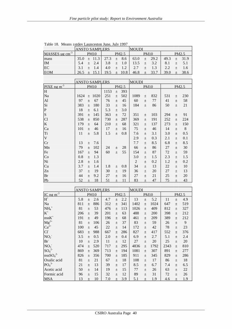
Fine particle pilot study: Report to Environment Australia
CSIRO Australia Page 40
Table 18. Means ±stdev Launceston June, July 1997ANSTO SAMPLERS MOUDI
MASSES µg cm-3 PM10 PM2.5 PM10 PM2.5mass 35.0 ± 11.3 27.3 ± 8.6 63.0 ± 29.2 49.3 ± 31.9IM 5.4 ± 2.4 3.8 ± 1.0 13.5 ± 3.2 8.1 ± 5.1EC 3.1 ± 1.4 4.0 ± 1.2 2.7 ± 1.3 2.2 ± 1.6EOM 26.5 ± 15.1 19.5 ± 10.8 46.8 ± 33.7 39.0 ± 38.6
ANSTO SAMPLERS MOUDIPIXE ng m-3 PM10 PM2.5 PM10 PM2.5H 1153 ± 393Na 1624 ± 1020 251 ± 502 1089 ± 832 531 ± 230Al 97 ± 67 76 ± 45 60 ± 77 41 ± 58Si 383 ± 180 33 ± 16 184 ± 86 50 ± 21P 18 ± 6.1 5.3 ± 3.0S 391 ± 145 363 ± 72 351 ± 103 294 ± 91Cl 538 ± 850 730 ± 287 369 ± 191 252 ± 224K 179 ± 64 210 ± 68 321 ± 137 273 ± 150Ca 101 ± 46 17 ± 16 75 ± 46 14 ± 8Ti 11 ± 5.8 1.5 ± 0.8 7.6 ± 3.1 3.0 ± 0.5V 2.9 ± 0.3 2.1 ± 0.1Cr 13 ± 7.6 7.7 ± 8.5 6.8 ± 8.5Mn 79 ± 102 24 ± 28 66 ± 86 27 ± 30Fe 167 ± 94 60 ± 55 154 ± 87 72 ± 59Co 0.8 ± 1.3 3.0 ± 1.5 2.3 ± 1.5Ni 2.8 ± 1.6 2 ± 0.2 1.2 ± 0.2Cu 3.7 ± 1.4 1.8 ± 0.8 34 ± 13 22 ± 10Zn 37 ± 19 30 ± 19 36 ± 20 27 ± 13Br 44 ± 9.2 27 ± 16 27 ± 21 25 ± 20Pb 52 ± 18 51 ± 11 83 ± 47 75 ± 43
ANSTO SAMPLERS MOUDIIC ng m-3 PM10 PM2.5 PM10 PM2.5H+ 5.8 ± 2.6 4.7 ± 2.2 13 ± 5.2 11 ± 4.9Na 811 ± 886 312 ± 341 1402 ± 1024 647 ± 519NH4
+ 81 ± 53 476 ± 113 1026 ± 409 812 ± 327K+ 206 ± 39 201 ± 63 488 ± 200 398 ± 212nssK+ 191 ± 49 196 ± 68 461 ± 209 389 ± 212Mg2+ 81 ± 106 26 ± 37 83 ± 59 26 ± 9Ca2+ 100 ± 45 22 ± 14 172 ± 42 78 ± 23Cl- 683 ± 988 667 ± 286 827 ± 417 552 ± 376NO2
- 3.5 ± 0.5 2.0 ± 0.4 6.9 ± 2.7 5.1 ± 2.4Br- 10 ± 2.9 11 ± 12 27 ± 20 25 ± 20NO3
- 474 ± 520 717 ± 295 4836 ± 1792 2343 ± 810SO4
2- 869 ± 369 713 ± 194 1081 ± 307 891 ± 277nssSO4
2- 826 ± 356 700 ± 185 911 ± 345 829 ± 286Oxalic acid 81 ± 21 67 ± 18 108 ± 17 86 ± 18PO4
3- 21 ± 13 39 ± 17 8.5 ± 6.7 7.4 ± 6.5Acetic acid 50 ± 14 19 ± 15 77 ± 26 63 ± 22Formic acid 96 ± 15 32 ± 12 89 ± 31 72 ± 26MSA 13 ± 10 7.0 ± 3.9 5.1 ± 1.9 4.6 ± 1.9
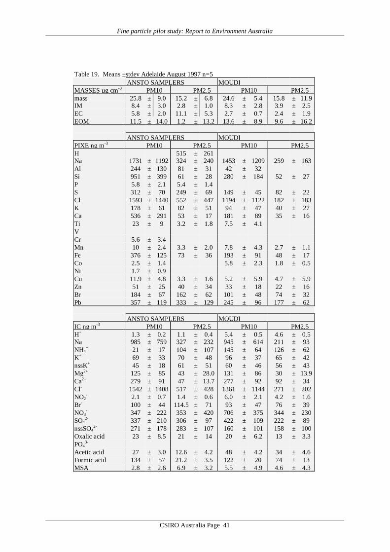
Fine particle pilot study: Report to Environment Australia
CSIRO Australia Page 41
Table 19. Means ±stdev Adelaide August 1997 n=5ANSTO SAMPLERS MOUDI
MASSES µg cm-3 PM10 PM2.5 PM10 PM2.5mass 25.8 ± 9.0 15.2 ± 6.8 24.6 ± 5.4 15.8 ± 11.9IM 8.4 ± 3.0 2.8 ± 1.0 8.3 ± 2.8 3.9 ± 2.5EC 5.8 ± 2.0 11.1 ± 5.3 2.7 ± 0.7 2.4 ± 1.9EOM 11.5 ± 14.0 1.2 ± 13.2 13.6 ± 8.9 9.6 ± 16.2
ANSTO SAMPLERS MOUDIPIXE ng m-3 PM10 PM2.5 PM10 PM2.5H 515 ± 261Na 1731 ± 1192 324 ± 240 1453 ± 1209 259 ± 163Al 244 ± 130 81 ± 31 42 ± 32Si 951 ± 399 61 ± 28 280 ± 184 52 ± 27P 5.8 ± 2.1 5.4 ± 1.4S 312 ± 70 249 ± 69 149 ± 45 82 ± 22Cl 1593 ± 1440 552 ± 447 1194 ± 1122 182 ± 183K 178 ± 61 82 ± 51 94 ± 47 40 ± 27Ca 536 ± 291 53 ± 17 181 ± 89 35 ± 16Ti 23 ± 9 3.2 ± 1.8 7.5 ± 4.1VCr 5.6 ± 3.4Mn 10 ± 2.4 3.3 ± 2.0 7.8 ± 4.3 2.7 ± 1.1Fe 376 ± 125 73 ± 36 193 ± 91 48 ± 17Co 2.5 ± 1.4 5.8 ± 2.3 1.8 ± 0.5Ni 1.7 ± 0.9Cu 11.9 ± 4.8 3.3 ± 1.6 5.2 ± 5.9 4.7 ± 5.9Zn 51 ± 25 40 ± 34 33 ± 18 22 ± 16Br 184 ± 67 162 ± 62 101 ± 48 74 ± 32Pb 357 ± 119 333 ± 129 245 ± 96 177 ± 62
ANSTO SAMPLERS MOUDIIC ng m-3 PM10 PM2.5 PM10 PM2.5H+ 1.3 ± 0.2 1.1 ± 0.4 5.4 ± 0.5 4.6 ± 0.5Na 985 ± 759 327 ± 232 945 ± 614 211 ± 93NH4
+ 21 ± 17 104 ± 107 145 ± 64 126 ± 62K+ 69 ± 33 70 ± 48 96 ± 37 65 ± 42nssK+ 45 ± 18 61 ± 51 60 ± 46 56 ± 43Mg2+ 125 ± 85 43 ± 28.0 131 ± 86 30 ± 13.9Ca2+ 279 ± 91 47 ± 13.7 277 ± 92 92 ± 34Cl- 1542 ± 1408 517 ± 428 1361 ± 1144 271 ± 202NO2
- 2.1 ± 0.7 1.4 ± 0.6 6.0 ± 2.1 4.2 ± 1.6Br- 100 ± 44 114.5 ± 71 93 ± 47 76 ± 39NO3
- 347 ± 222 353 ± 420 706 ± 375 344 ± 230SO4
2- 337 ± 210 306 ± 97 422 ± 109 222 ± 89nssSO4
2- 271 ± 178 283 ± 107 160 ± 101 158 ± 100Oxalic acid 23 ± 8.5 21 ± 14 20 ± 6.2 13 ± 3.3PO4
3-
Acetic acid 27 ± 3.0 12.6 ± 4.2 48 ± 4.2 34 ± 4.6Formic acid 134 ± 57 21.2 ± 3.5 122 ± 20 74 ± 13MSA 2.8 ± 2.6 6.9 ± 3.2 5.5 ± 4.9 4.6 ± 4.3

Fine particle pilot study: Report to Environment Australia
CSIRO Australia Page 42
Table 20. Mean PM2.5 mass concentrations (measured by TEOM), bsp and bspd
(measured by nephelometer) and CN measured by TSI-UCPC# (Sydney) and CSIROCN counter& (Melbourne, Canberra, Launceston and Adelaide); n = number of daysof data.
TEOM PM2.5 bsp bspd CN
µgm-3 10-5 m-1 10-5 m-1 103 cm-3
Sydney 27 ± 5 n=18#
Brisbane
Melbourne 8 ± 3 n=12 2.8 ± 1.1 n=7 1.6 ± 1.1 n=27 37 ± 79 n=28&
Canberra 19 ± 10 n=20 9.6 ± 9.3 n=26 7.0 ± 6.5 n=24 21 ± 72 n=33&
Launceston 36 ± 25 n=46 21 ± 13 n=44 13.5 ± 8.6 n=44 24 ± 9 n=50&
Adelaide 11 ± 25 n=25 3.0 ± 1.2 n=24 1.9 ± 0.9 n=24 60 ± 23 n=25&
7.2 Aerosol Composition as a Function of Particle Size (MOUDI Data)
The MOUDI data provide information on the distribution with size of aerosolproperties, at a level of detail hitherto unavailable in Australia. The initial presentation of sizedistributions in this chapter is made in Figures 12 – 17. These figures illustrate the capabilityof the MOUDI to reveal definitively the characteristic size ranges inhabited by specificelements and chemical species. The Figures show the distribution with size of tracers forparticular aerosol sources, such as Pb, Br and EC which in the Sydney atmosphere deriveprimarily from automotive emissions (Figure 12). Figure 13 shows distributions for strongacids (sulfuric and nitric) derived from atmospheric oxidation of SO2 and NOx, along with thecounter ions H+ and NH4
+, in a Brisbane sample.
0
500
1000
1500
2000
2500
3000
0.01 0.1 1 10 100diameter, µm
Elem
enta
l Car
bon
dM/d
logd
, ngm
-3
0
20
40
60
80
100
120
140
160
Pb, B
r dM
/dlo
gd, n
gm-3
Elemental Carbon (EC)
Pb
Br
Figure 12. Mass distribution of automotive tracers, Sydney aerosol.
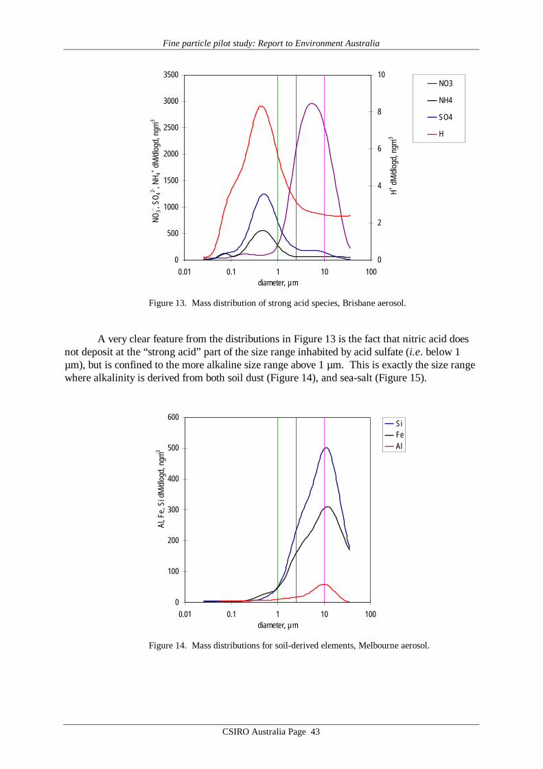
Fine particle pilot study: Report to Environment Australia
CSIRO Australia Page 43
0
500
1000
1500
2000
2500
3000
3500
0.01 0.1 1 10 100diameter, µm
NO3- , S
O 42-
, NH 4
+ dM
/dlo
gd, n
gm-3
0
2
4
6
8
10
H+ dM
/dlo
gd, n
gm-3
NO3
NH4
SO4
H
Figure 13. Mass distribution of strong acid species, Brisbane aerosol.
A very clear feature from the distributions in Figure 13 is the fact that nitric acid doesnot deposit at the “strong acid” part of the size range inhabited by acid sulfate (i.e. below 1µm), but is confined to the more alkaline size range above 1 µm. This is exactly the size rangewhere alkalinity is derived from both soil dust (Figure 14), and sea-salt (Figure 15).
0
100
200
300
400
500
600
0.01 0.1 1 10 100diameter, µm
Al, F
e, S
i dM
/dlo
gd, n
gm-3
SiFeAl
Figure 14. Mass distributions for soil-derived elements, Melbourne aerosol.

Fine particle pilot study: Report to Environment Australia
CSIRO Australia Page 44
0
500
1000
1500
2000
2500
3000
3500
0.01 0.1 1 10 100diameter, µm
Cl- , N
a+ dM
/dlo
gd, n
gm-3
0
50
100
150
200
250
300
Mg2+
dM
/dlo
gd, n
gm-3
Na
Cl
Mg
Figure 15. Mass distributions for sea-salt-derived elements, Adelaide aerosol.
Finally, Figure 16 provides evidence of the strong role played by wood-burning (nssK+
is a tracer for smoke from biomass combustion) in dominating the aerosol mass distributionduring winter in Launceston, while Figure 17 reveals a more complex picture of thecontributions made by different major aerosol components in an aerosol sample fromCanberra.
0
10
20
30
40
50
60
70
0.01 0.1 1 10 100diameter, µm
Mas
s dM
/dlo
gd, µ
gm-3
0
100
200
300
400
500
600
nssK
+ dM/d
logd
, ngm
-3
GravimetricMass
nssK
Figure 16. Mass distributions for nssK+ and total mass, Launceston aerosol.

Fine particle pilot study: Report to Environment Australia
CSIRO Australia Page 45
0
5
10
15
20
0.01 0.1 1 10 100diameter, µm
dM/d
logd
, µg
m-3
Gravimetric MassEOMIMEC
Figure 17. Major mass components, Canberra aerosol. EOM = estimatedorganic mass; IM = inorganic mass; EC = elemental carbon mass.
Since the MOUDI provides simultaneous information on different size ranges, such asthe PM10, PM2.5 and PM1 size ranges delineated by the vertical lines in Figures 13 – 17, aself-consistent (i.e. from within a single sample) picture of the relationship between thedifferent PM fractions is readily derived. Figure 18 contains a plot of PM2.5 vs PM10 from allMOUDI samples, revealing a very clear structural relationship, a particular feature of which isa decreasing role for PM2.5 as total aerosol mass (i.e. PM10 and PM2.5) levels decrease. Thelatter point is more clearly evident in Figure 19, which reveals a systematic variation the ratioof PM2.5/PM10 as a function of PM2.5.
0
20
40
60
80
100
120
0 20 40 60 80 100 120
PM10, µgm-3
PM2.
5, µ
gm-3
Figure 18. PM2.5 vs PM10 data, all sites.
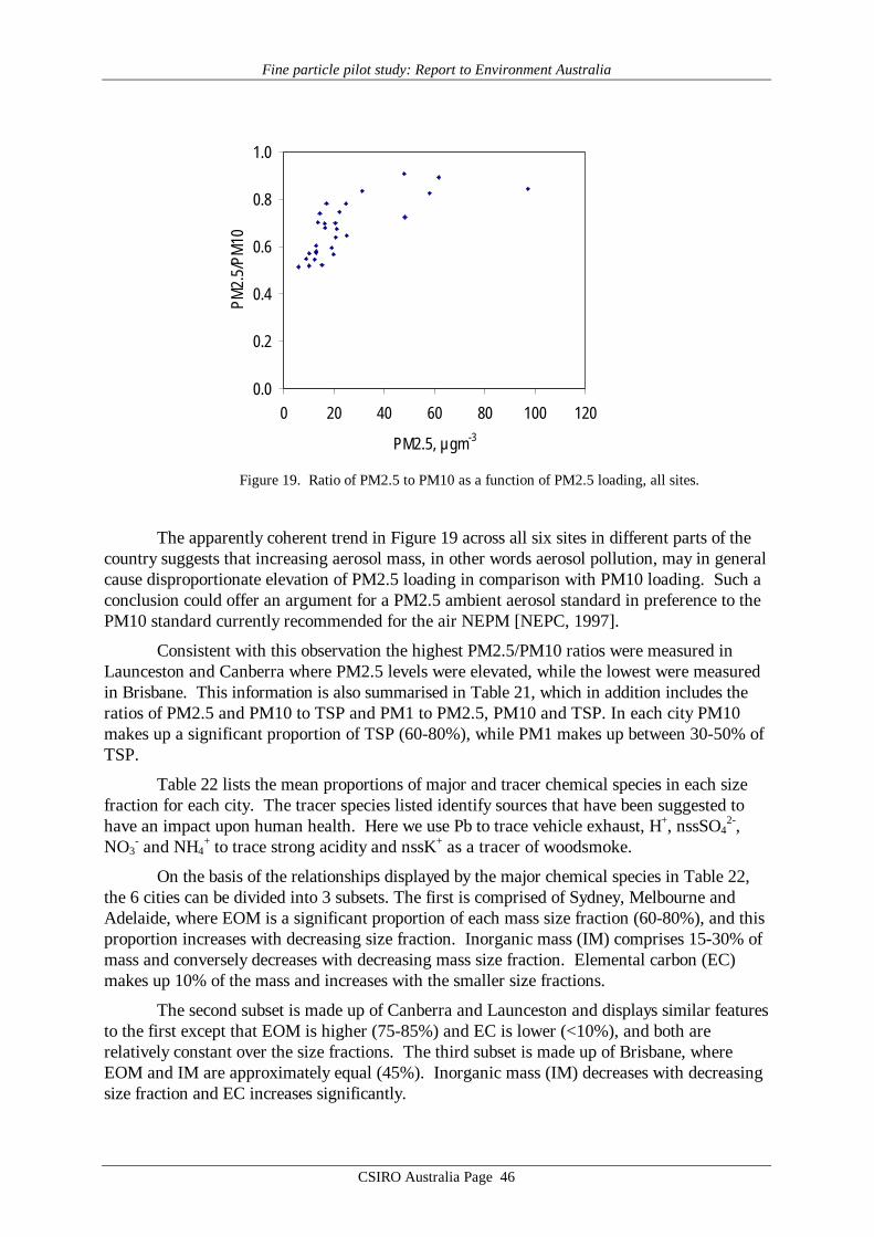
Fine particle pilot study: Report to Environment Australia
CSIRO Australia Page 46
0.0
0.2
0.4
0.6
0.8
1.0
0 20 40 60 80 100 120
PM2.5, µgm-3
PM2.
5/PM
10
Figure 19. Ratio of PM2.5 to PM10 as a function of PM2.5 loading, all sites.
The apparently coherent trend in Figure 19 across all six sites in different parts of thecountry suggests that increasing aerosol mass, in other words aerosol pollution, may in generalcause disproportionate elevation of PM2.5 loading in comparison with PM10 loading. Such aconclusion could offer an argument for a PM2.5 ambient aerosol standard in preference to thePM10 standard currently recommended for the air NEPM [NEPC, 1997].
Consistent with this observation the highest PM2.5/PM10 ratios were measured inLaunceston and Canberra where PM2.5 levels were elevated, while the lowest were measuredin Brisbane. This information is also summarised in Table 21, which in addition includes theratios of PM2.5 and PM10 to TSP and PM1 to PM2.5, PM10 and TSP. In each city PM10makes up a significant proportion of TSP (60-80%), while PM1 makes up between 30-50% ofTSP.
Table 22 lists the mean proportions of major and tracer chemical species in each sizefraction for each city. The tracer species listed identify sources that have been suggested tohave an impact upon human health. Here we use Pb to trace vehicle exhaust, H+, nssSO4
2-,NO3
- and NH4+ to trace strong acidity and nssK+ as a tracer of woodsmoke.
On the basis of the relationships displayed by the major chemical species in Table 22,the 6 cities can be divided into 3 subsets. The first is comprised of Sydney, Melbourne andAdelaide, where EOM is a significant proportion of each mass size fraction (60-80%), and thisproportion increases with decreasing size fraction. Inorganic mass (IM) comprises 15-30% ofmass and conversely decreases with decreasing mass size fraction. Elemental carbon (EC)makes up 10% of the mass and increases with the smaller size fractions.
The second subset is made up of Canberra and Launceston and displays similar featuresto the first except that EOM is higher (75-85%) and EC is lower (<10%), and both arerelatively constant over the size fractions. The third subset is made up of Brisbane, whereEOM and IM are approximately equal (45%). Inorganic mass (IM) decreases with decreasingsize fraction and EC increases significantly.
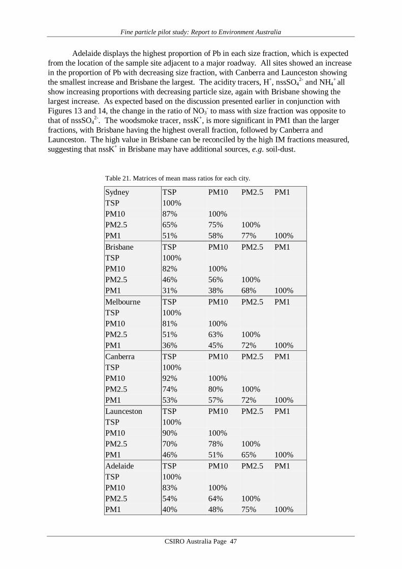
Fine particle pilot study: Report to Environment Australia
CSIRO Australia Page 47
Adelaide displays the highest proportion of Pb in each size fraction, which is expectedfrom the location of the sample site adjacent to a major roadway. All sites showed an increasein the proportion of Pb with decreasing size fraction, with Canberra and Launceston showingthe smallest increase and Brisbane the largest. The acidity tracers, H+, nssSO4
2- and NH4+ all
show increasing proportions with decreasing particle size, again with Brisbane showing thelargest increase. As expected based on the discussion presented earlier in conjunction withFigures 13 and 14, the change in the ratio of NO3
- to mass with size fraction was opposite tothat of nssSO4
2-. The woodsmoke tracer, nssK+, is more significant in PM1 than the largerfractions, with Brisbane having the highest overall fraction, followed by Canberra andLaunceston. The high value in Brisbane can be reconciled by the high IM fractions measured,suggesting that nssK+ in Brisbane may have additional sources, e.g. soil-dust.
Table 21. Matrices of mean mass ratios for each city.
Sydney TSP PM10 PM2.5 PM1TSP 100%PM10 87% 100%PM2.5 65% 75% 100%PM1 51% 58% 77% 100%Brisbane TSP PM10 PM2.5 PM1TSP 100%PM10 82% 100%PM2.5 46% 56% 100%PM1 31% 38% 68% 100%Melbourne TSP PM10 PM2.5 PM1TSP 100%PM10 81% 100%PM2.5 51% 63% 100%PM1 36% 45% 72% 100%Canberra TSP PM10 PM2.5 PM1TSP 100%PM10 92% 100%PM2.5 74% 80% 100%PM1 53% 57% 72% 100%Launceston TSP PM10 PM2.5 PM1TSP 100%PM10 90% 100%PM2.5 70% 78% 100%PM1 46% 51% 65% 100%Adelaide TSP PM10 PM2.5 PM1TSP 100%PM10 83% 100%PM2.5 54% 64% 100%PM1 40% 48% 75% 100%

Fine particle pilot study: Report to Environment Australia
CSIRO Australia Page 48
Table 22. Mean proportion of major and tracer chemical species to masssize fraction in each city.
SydneyMajors TSP PM10 PM2.5 PM1Mass 100% 100% 100% 100%EOM 70% 69% 72% 73%IM-EC 21% 21% 16% 15%EC 9% 10% 11% 12%TracersPb 0.34% 0.38% 0.46% 0.50%H+ 0.04% 0.04% 0.05% 0.05%nssSO4
2- 3.05% 3.45% 4.48% 4.95%NO3
- 2.95% 3.00% 1.93% 1.50%NH4
+ 1.41% 1.59% 2.06% 2.32%nssK+ 0.43% 0.46% 0.57% 0.62%BrisbaneMajors TSP PM10 PM2.5 PM1Mass 100% 100% 100% 100%EOM 46% 46% 50% 53%IM-EC 47% 45% 36% 31%EC 7% 9% 14% 17%TracersPb 0.12% 0.13% 0.20% 0.25%H+ 0.04% 0.05% 0.07% 0.08%nssSO4
2- 3.16% 3.83% 6.62% 8.31%NO3
- 13.84% 12.55% 7.97% 5.02%NH4
+ 1.61% 1.87% 3.09% 3.99%nssK+ 1.04% 1.02% 1.32% 1.37%MelbourneMajors TSP PM10 PM2.5 PM1Mass 100% 100% 100% 100%EOM 64% 63% 71% 74%IM-EC 29% 28% 18% 14%EC 7% 8% 10% 11%TracersPb 0.20% 0.25% 0.34% 0.38%H+ 0.03% 0.03% 0.04% 0.04%nssSO4
2- 2.47% 2.95% 4.31% 5.42%NO3
- 3.62% 3.79% 2.30% 0.97%NH4
+ 0.70% 0.84% 1.25% 1.65%nssK+ 0.21% 0.23% 0.32% 0.38%CanberraMajors TSP PM10 PM2.5 PM1Mass 100% 100% 100% 100%EOM 78% 79% 83% 83%IM-EC 14% 13% 9% 8%EC 8% 8% 8% 9%TracersPb 0.22% 0.24% 0.27% 0.29%H+ 0.03% 0.03% 0.03% 0.03%nssSO4
2- 2.81% 3.01% 3.65% 4.06%NO3
- 3.20% 2.99% 1.45% 1.04%NH4
+ 1.17% 1.25% 1.54% 1.83%nssK+ 0.56% 0.58% 0.64% 0.70%
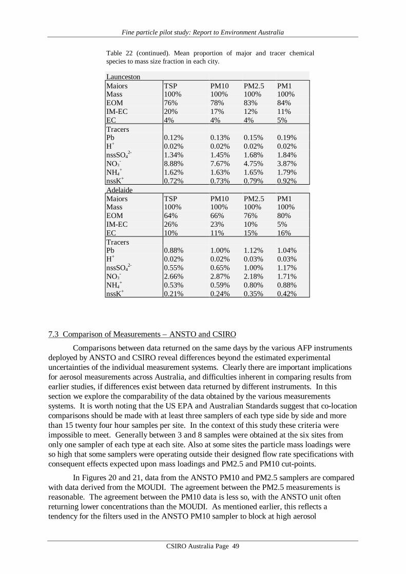
Fine particle pilot study: Report to Environment Australia
CSIRO Australia Page 49
Table 22 (continued). Mean proportion of major and tracer chemicalspecies to mass size fraction in each city.
LauncestonMajors TSP PM10 PM2.5 PM1Mass 100% 100% 100% 100%EOM 76% 78% 83% 84%IM-EC 20% 17% 12% 11%EC 4% 4% 4% 5%TracersPb 0.12% 0.13% 0.15% 0.19%H+ 0.02% 0.02% 0.02% 0.02%nssSO4
2- 1.34% 1.45% 1.68% 1.84%NO3
- 8.88% 7.67% 4.75% 3.87%NH4
+ 1.62% 1.63% 1.65% 1.79%nssK+ 0.72% 0.73% 0.79% 0.92%AdelaideMajors TSP PM10 PM2.5 PM1Mass 100% 100% 100% 100%EOM 64% 66% 76% 80%IM-EC 26% 23% 10% 5%EC 10% 11% 15% 16%TracersPb 0.88% 1.00% 1.12% 1.04%H+ 0.02% 0.02% 0.03% 0.03%nssSO4
2- 0.55% 0.65% 1.00% 1.17%NO3
- 2.66% 2.87% 2.18% 1.71%NH4
+ 0.53% 0.59% 0.80% 0.88%nssK+ 0.21% 0.24% 0.35% 0.42%
7.3 Comparison of Measurements – ANSTO and CSIRO
Comparisons between data returned on the same days by the various AFP instrumentsdeployed by ANSTO and CSIRO reveal differences beyond the estimated experimentaluncertainties of the individual measurement systems. Clearly there are important implicationsfor aerosol measurements across Australia, and difficulties inherent in comparing results fromearlier studies, if differences exist between data returned by different instruments. In thissection we explore the comparability of the data obtained by the various measurementssystems. It is worth noting that the US EPA and Australian Standards suggest that co-locationcomparisons should be made with at least three samplers of each type side by side and morethan 15 twenty four hour samples per site. In the context of this study these criteria wereimpossible to meet. Generally between 3 and 8 samples were obtained at the six sites fromonly one sampler of each type at each site. Also at some sites the particle mass loadings wereso high that some samplers were operating outside their designed flow rate specifications withconsequent effects expected upon mass loadings and PM2.5 and PM10 cut-points.
In Figures 20 and 21, data from the ANSTO PM10 and PM2.5 samplers are comparedwith data derived from the MOUDI. The agreement between the PM2.5 measurements isreasonable. The agreement between the PM10 data is less so, with the ANSTO unit oftenreturning lower concentrations than the MOUDI. As mentioned earlier, this reflects atendency for the filters used in the ANSTO PM10 sampler to block at high aerosol

Fine particle pilot study: Report to Environment Australia
CSIRO Australia Page 50
concentrations, slowing the flow rate into the sampler and thus changing the collectioncharacteristics of the unit. Side by side comparisons of PM2.5 data taken on the ANSTOstacked sampler and the ANSTO cyclone sampler over a 2 year period involving 200 filters hasproduced better correlations than those shown in Fig. 21. In these previous comparisons, thestacked filter to cyclone PM2.5 ratio was (0.89±0.19) for the mass and (0.95±0.12) for thesulfur concentrations.
Figures 22 and 23 compare the CSIRO PM2.5 TEOM data with PM2.5 data derivedfrom the MOUDI and ANSTO samplers. Both the MOUDI and ANSTO instrument measuredgreater mass than the TEOM. This probably results from the loss of mass by the TEOM fromvolatilisation of semi-volatile material, as the inlet of the TEOM was heated to 50°C(Melbourne) or 35°C (subsequent cities). Figure 24 displays a comparison between the Solar-Vol PM2.5 sampler and the MOUDI. The agreement between these two instruments is good.
y = 0.62 (0.26)x + 5.41(7.54)R2 = 0.56
0
20
40
60
80
0 20 40 60 80MOUDI PM10, µgm-3
ANST
O P
M10
,µgm
-3
Figure 20. Relative performance of ANSTO PM10 sampler and the MOUDI.Numbers in parenthesis are the 95% confidence ranges.
y = 1.22(0.17)x - 8.10(5.3)R2 = 0.91
0
30
60
90
120
0 30 60 90 120MOUDI PM2.5, µgm-3
ANST
O P
M2.
5,µg
m-3
Figure 21. Relative performance of ANSTO PM2.5 sampler and the MOUDI.Numbers in parenthesis are the 95% confidence ranges.

Fine particle pilot study: Report to Environment Australia
CSIRO Australia Page 51
y = 0.71(0.08)x + 0.17(2.96)R2 = 0.97
0
20
40
60
80
100
0 20 40 60 80 100MOUDI PM2.5, µgm-3
TEO
M P
M2.
5,µg
m-3
Figure 22. Relative performance of CSIRO PM2.5 TEOM and the MOUDI.Numbers in parenthesis are the 95% confidence ranges.
y = 0.56(0.10)x + 4.56(4.05)R2 = 0.93
0
20
40
60
80
100
0 20 40 60 80 100ANSTO PM2.5, µgm-3
TEO
M P
M2.
5,µg
m-3
Figure 23. Relative performance of CSIRO PM2.5 TEOM and the ANSTOPM2.5 sampler. Numbers in parenthesis are the 95% confidence ranges.

Fine particle pilot study: Report to Environment Australia
CSIRO Australia Page 52
y = 1.06(0.14)x + 0.51(5.24)R2 = 0.97
0
30
60
90
120
0 30 60 90 120MOUDI PM2.5, µgm-3
Sola
rvol
PM
2.5,
µgm-3
Figure 24. Relative performance of Solar-Vol PM2.5 sampler and theMOUDI. Numbers in parenthesis are the 95% confidence ranges.
The next comparison is made between the two continuously recording aerosolinstruments, the nephelometer and the TEOM. Figure 25 shows an example of the relationshipbetween bspd and PM2.5 for hourly values. The relationships for each of the four cities inwhich both devices operated are summarised in Table 23. A linear relationship exists betweenthe two parameters, with varying degrees of agreement at each site. It is notable that theLaunceston and Canberra data in Table 23 clearly exhibit one slope, with the Melbourne andAdelaide data exhibiting another slope, a factor of 2 – 3 different. In later discussion it will beshown that these differences in scattering-mass relationship are caused primarily by systematicdifferences in aerosol size distribution caused by different dominant source types inLaunceston/Canberra (smoke) and Melbourne/Adelaide (urban/automobiles).
bspd = 0.41TEOM + 2.14R2 = 0.70
0
20
40
60
80
100
0 50 100 150 200 250
TEOM PM2.5, µgm-3
b spd
, 10-5
m-1
Figure 25. Relationship between bspd (measured by Nephelometer) andPM2.5 (measured by TEOM) for hourly values at Launceston.
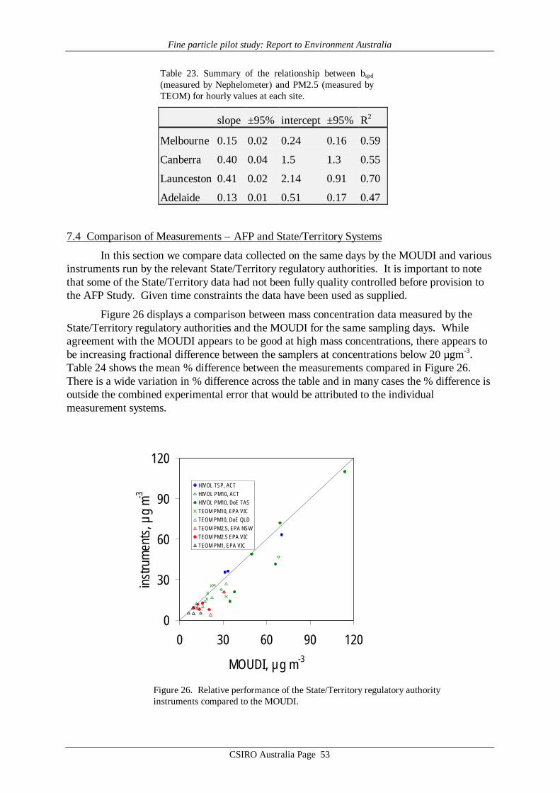
Fine particle pilot study: Report to Environment Australia
CSIRO Australia Page 53
Table 23. Summary of the relationship between bspd
(measured by Nephelometer) and PM2.5 (measured byTEOM) for hourly values at each site.
slope ±95% intercept ±95% R2
Melbourne 0.15 0.02 0.24 0.16 0.59
Canberra 0.40 0.04 1.5 1.3 0.55
Launceston 0.41 0.02 2.14 0.91 0.70
Adelaide 0.13 0.01 0.51 0.17 0.47
7.4 Comparison of Measurements – AFP and State/Territory Systems
In this section we compare data collected on the same days by the MOUDI and variousinstruments run by the relevant State/Territory regulatory authorities. It is important to notethat some of the State/Territory data had not been fully quality controlled before provision tothe AFP Study. Given time constraints the data have been used as supplied.
Figure 26 displays a comparison between mass concentration data measured by theState/Territory regulatory authorities and the MOUDI for the same sampling days. Whileagreement with the MOUDI appears to be good at high mass concentrations, there appears tobe increasing fractional difference between the samplers at concentrations below 20 µgm-3.Table 24 shows the mean % difference between the measurements compared in Figure 26.There is a wide variation in % difference across the table and in many cases the % difference isoutside the combined experimental error that would be attributed to the individualmeasurement systems.
0
30
60
90
120
0 30 60 90 120
MOUDI, µg m-3
inst
rum
ents
, µg
m-3
HIVOL TSP, ACTHIVOL PM10, ACTHIVOL PM10, DoE TASTEOM PM10, EPA VICTEOM PM10, DoE QLDTEOM PM2.5, EPA NSWTEOM PM2.5 EPA VICTEOM PM1, EPA VIC
Figure 26. Relative performance of the State/Territory regulatory authorityinstruments compared to the MOUDI.
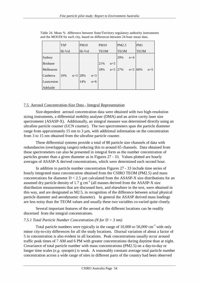
Fine particle pilot study: Report to Environment Australia
CSIRO Australia Page 54
Table 24. Mean % difference between State/Territory regulatory authority instrumentsand the MOUDI for each city, based on differences between 24 hour mean data.
TSP PM10 PM10 PM2.5 PM1
Hi-Vol Hi-Vol TEOM TEOM TEOM
Sydney 29% n=4
Brisbane 21% n=5
Melbourne 18% n=5 27% n=5 60% n=5
Canberra 10% n=3 28% n=3
Launceston 14% n=6
Adelaide
7.5 Aerosol Concentration-Size Data - Integral Representation
Size-dependent aerosol concentration data were obtained with two high-resolutionsizing instruments, a differential mobility analyser (DMA) and an active cavity laser sizespectrometer (ASASP-X). Additionally, an integral measure was determined directly using anultrafine particle counter (UCN counter). The two spectrometers span the particle diameterrange from approximately 15 nm to 3 µm, with additional information on the concentrationfrom 3 to 15 nm obtained from the ultrafine particle counter.
These differential systems provide a total of 88 particle size channels of data withredundancies (overlapping ranges) reducing this to around 65 channels. Data obtained fromthese spectrometers can also be presented in integral form as the number concentration ofparticles greater than a given diameter as in Figures 27 - 33. Values plotted are hourlyaverages of ASASP-X derived concentrations, which were determined each second hour.
In addition to particle number concentration Figures 27 - 33 include time series ofhourly integrated mass concentration obtained from the CSIRO TEOM (PM2.5) and massconcentrations for diameter D < 2.5 µm calculated from the ASASP-X size distributions for anassumed dry particle density of 1.7 g cm-3 (all masses derived from the ASASP-X sizedistribution measurements that are discussed here, and elsewhere in the text, were obtained inthis way, and are designated as M2.5, in recognition of the difference between actual physicalparticle diameter and aerodynamic diameter). In general the ASASP derived mass loadingsare less noisy than the TEOM values and usually these two variables co-varied quite closely.
Several important features of the aerosol at the different locations can be readilydiscerned from the integral concentrations.
7.5.1 Total Particle Number Concentration (N for D > 3 nm)
Total particle numbers were typically in the range of 10,000 to 50,000 cm-3 with onlyminor city-to-city differences for all the study locations. Diurnal variation of about a factor of5 in concentration is also evident in all locations. Peak concentrations usually occur aroundtraffic peak times of 7 AM and 6 PM with greater concentrations during daytime than at night.Covariance of total particle number with mass concentrations (PM2.5) on a day-to-day orlonger time scales (e.g. synoptic) is weak. A reasonably constant average total particle numberconcentration across a wide range of sites in different parts of the country had been observed
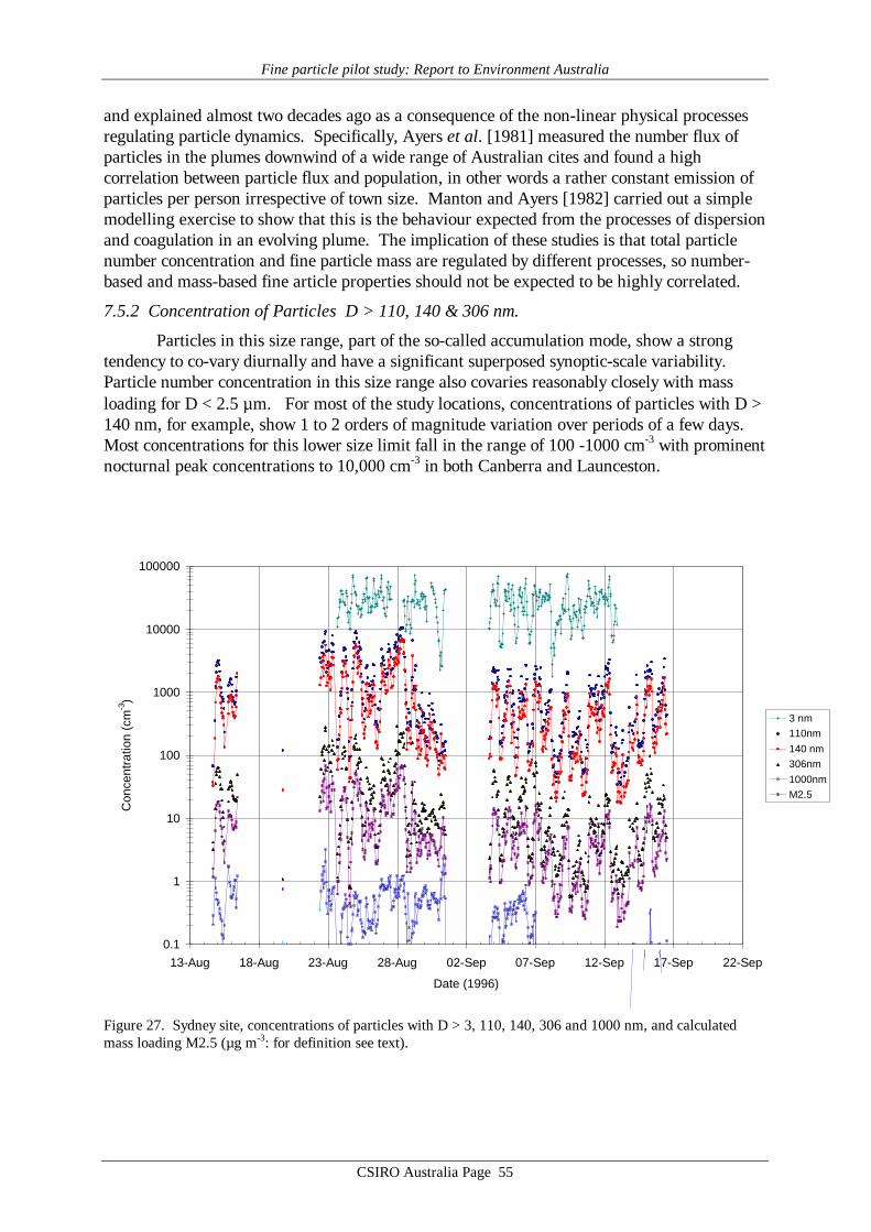
Fine particle pilot study: Report to Environment Australia
CSIRO Australia Page 55
and explained almost two decades ago as a consequence of the non-linear physical processesregulating particle dynamics. Specifically, Ayers et al. [1981] measured the number flux ofparticles in the plumes downwind of a wide range of Australian cites and found a highcorrelation between particle flux and population, in other words a rather constant emission ofparticles per person irrespective of town size. Manton and Ayers [1982] carried out a simplemodelling exercise to show that this is the behaviour expected from the processes of dispersionand coagulation in an evolving plume. The implication of these studies is that total particlenumber concentration and fine particle mass are regulated by different processes, so number-based and mass-based fine article properties should not be expected to be highly correlated.
7.5.2 Concentration of Particles D > 110, 140 & 306 nm.
Particles in this size range, part of the so-called accumulation mode, show a strongtendency to co-vary diurnally and have a significant superposed synoptic-scale variability.Particle number concentration in this size range also covaries reasonably closely with massloading for D < 2.5 µm. For most of the study locations, concentrations of particles with D >140 nm, for example, show 1 to 2 orders of magnitude variation over periods of a few days.Most concentrations for this lower size limit fall in the range of 100 -1000 cm-3 with prominentnocturnal peak concentrations to 10,000 cm-3 in both Canberra and Launceston.
0.1
1
10
100
1000
10000
100000
13-Aug 18-Aug 23-Aug 28-Aug 02-Sep 07-Sep 12-Sep 17-Sep 22-Sep
Date (1996)
Con
cent
ratio
n (c
m-3
)
3 nm110nm140 nm306nm1000nmM2.5
Figure 27. Sydney site, concentrations of particles with D > 3, 110, 140, 306 and 1000 nm, and calculatedmass loading M2.5 (µg m-3: for definition see text).

Fine particle pilot study: Report to Environment Australia
CSIRO Australia Page 56
0.1
1
10
100
1000
10000
100000
30-Sep 10-Oct 20-Oct 30-Oct 9-Nov 19-Nov
Date (1996)
Con
cent
ratio
n (c
m-3
)
3nm110nm140 nm306 nm1000 nmM2.5
Figure 28. Brisbane site, concentrations of particles with D > 3, 110, 140, 306 and 1000 nm, and calculatedmass loading M2.5 (µg m-3: for definition see text).
0.1
1
10
100
1000
10000
100000
02-Apr 07-Apr 12-Apr 17-Apr 22-Apr 27-Apr
Date (1997)
Con
cent
ratio
n (c
m-3
)
3nm110nm140nm306nm1000nmM2.5TEOM
Figure 29. Melbourne site, concentrations of particles with D > 3, 110, 140, 306 and 1000 nm, and calculatedmass loading M2.5 (µg m-3: for definition see text). Also included, PM2.5 mass loading (µg m-3) from theCSIRO TEOM.

Fine particle pilot study: Report to Environment Australia
CSIRO Australia Page 57
0.1
1
10
100
1000
10000
100000
03-May 08-May 13-May 18-May 23-May 28-May 02-Jun
Date (1997)
Con
cent
ratio
n (c
m-3
)
3nm110nm140nm306nm1000nmM2.5TEOM
Figure 30. Canberra site, concentrations of particles with D > 3, 110, 140, 306 and 1000 nm, and calculatedmass loading M2.5 (µg m-3: for definition see text). Also included, PM2.5 mass loading (µg m-3) from theCSIRO TEOM.
0.1
1
10
100
1000
10000
100000
10-Jun 15-Jun 20-Jun 25-Jun 30-Jun 05-Jul
Date (1997)
Con
cent
ratio
n (c
m-3
)
3nm110nm140nm306nm1000nmM2.5TEOM
Figure 31. Launceston site, concentrations of particles with D > 3, 110, 140, 306 and 1000 nm, and calculatedmass loading M2.5 (µg m-3: for definition see text). Also included, PM2.5 mass loading (µg m-3) from theCSIRO TEOM.
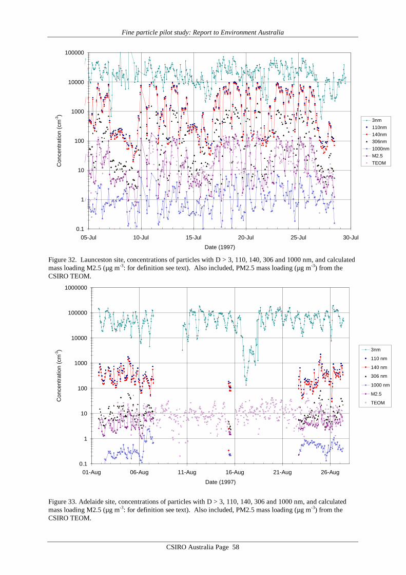
Fine particle pilot study: Report to Environment Australia
CSIRO Australia Page 58
0.1
1
10
100
1000
10000
100000
05-Jul 10-Jul 15-Jul 20-Jul 25-Jul 30-Jul
Date (1997)
Con
cent
ratio
n (c
m-3
)
3nm110nm140nm306nm1000nmM2.5TEOM
Figure 32. Launceston site, concentrations of particles with D > 3, 110, 140, 306 and 1000 nm, and calculatedmass loading M2.5 (µg m-3: for definition see text). Also included, PM2.5 mass loading (µg m-3) from theCSIRO TEOM.
0.1
1
10
100
1000
10000
100000
1000000
01-Aug 06-Aug 11-Aug 16-Aug 21-Aug 26-Aug
Date (1997)
Con
cent
ratio
n (c
m-3
) 3nm
110 nm
140 nm
306 nm
1000 nm
M2.5
TEOM
Figure 33. Adelaide site, concentrations of particles with D > 3, 110, 140, 306 and 1000 nm, and calculatedmass loading M2.5 (µg m-3: for definition see text). Also included, PM2.5 mass loading (µg m-3) from theCSIRO TEOM.
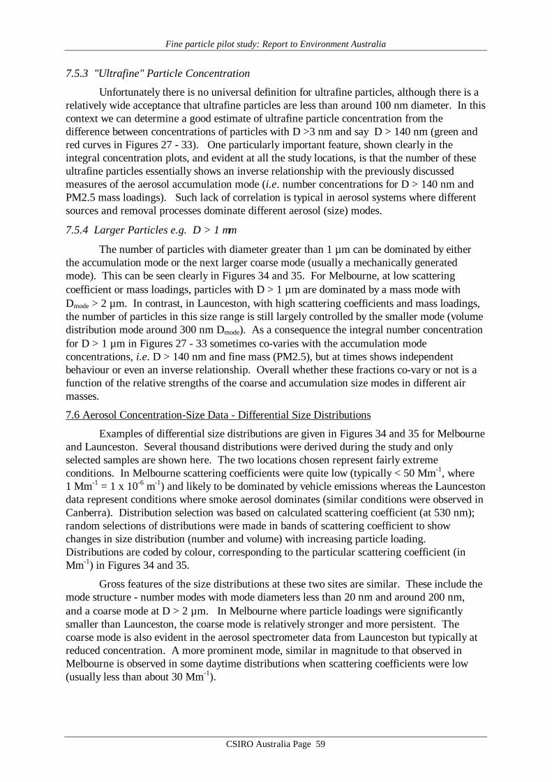
Fine particle pilot study: Report to Environment Australia
CSIRO Australia Page 59
7.5.3 "Ultrafine" Particle Concentration
Unfortunately there is no universal definition for ultrafine particles, although there is arelatively wide acceptance that ultrafine particles are less than around 100 nm diameter. In thiscontext we can determine a good estimate of ultrafine particle concentration from thedifference between concentrations of particles with D >3 nm and say D > 140 nm (green andred curves in Figures 27 - 33). One particularly important feature, shown clearly in theintegral concentration plots, and evident at all the study locations, is that the number of theseultrafine particles essentially shows an inverse relationship with the previously discussedmeasures of the aerosol accumulation mode (i.e. number concentrations for D > 140 nm andPM2.5 mass loadings). Such lack of correlation is typical in aerosol systems where differentsources and removal processes dominate different aerosol (size) modes.
7.5.4 Larger Particles e.g. D > 1 µm
The number of particles with diameter greater than 1 µm can be dominated by eitherthe accumulation mode or the next larger coarse mode (usually a mechanically generatedmode). This can be seen clearly in Figures 34 and 35. For Melbourne, at low scatteringcoefficient or mass loadings, particles with D > 1 µm are dominated by a mass mode withDmode > 2 µm. In contrast, in Launceston, with high scattering coefficients and mass loadings,the number of particles in this size range is still largely controlled by the smaller mode (volumedistribution mode around 300 nm Dmode). As a consequence the integral number concentrationfor D > 1 µm in Figures 27 - 33 sometimes co-varies with the accumulation modeconcentrations, i.e. D > 140 nm and fine mass (PM2.5), but at times shows independentbehaviour or even an inverse relationship. Overall whether these fractions co-vary or not is afunction of the relative strengths of the coarse and accumulation size modes in different airmasses.
7.6 Aerosol Concentration-Size Data - Differential Size Distributions
Examples of differential size distributions are given in Figures 34 and 35 for Melbourneand Launceston. Several thousand distributions were derived during the study and onlyselected samples are shown here. The two locations chosen represent fairly extremeconditions. In Melbourne scattering coefficients were quite low (typically < 50 Mm-1, where1 Mm-1 = 1 x 10⁻⁶ m-1) and likely to be dominated by vehicle emissions whereas the Launcestondata represent conditions where smoke aerosol dominates (similar conditions were observed inCanberra). Distribution selection was based on calculated scattering coefficient (at 530 nm);random selections of distributions were made in bands of scattering coefficient to showchanges in size distribution (number and volume) with increasing particle loading.Distributions are coded by colour, corresponding to the particular scattering coefficient (inMm-1) in Figures 34 and 35.
Gross features of the size distributions at these two sites are similar. These include themode structure - number modes with mode diameters less than 20 nm and around 200 nm,and a coarse mode at D > 2 µm. In Melbourne where particle loadings were significantlysmaller than Launceston, the coarse mode is relatively stronger and more persistent. Thecoarse mode is also evident in the aerosol spectrometer data from Launceston but typically atreduced concentration. A more prominent mode, similar in magnitude to that observed inMelbourne is observed in some daytime distributions when scattering coefficients were low(usually less than about 30 Mm-1).
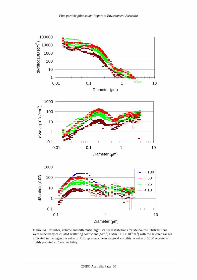
Fine particle pilot study: Report to Environment Australia
CSIRO Australia Page 60
1
10
100
1000
10000
100000
0.01 0.1 1 10
Diameter (µm)
dN/d
log1
0D (c
m-3
)
0.1
1
10
100
1000
0.01 0.1 1 10
Diameter (µm)
dV/d
log1
0D (c
m-3
)
0.1
1
10
100
1000
0.1 1 10
Diameter (µm)
dSca
t/dlo
g10D
~ 100~ 50~ 25< 10
Figure 34. Number, volume and differential light scatter distributions for Melbourne. Distributionswere selected by calculated scattering coefficient (Mm-1; 1 Mm-1 = 1 x 10⁻⁶ m-1) with the selected rangesindicated in the legend; a value of <10 represents clean air/good visibility; a value of ≥100 representshighly polluted air/poor visibility.

Fine particle pilot study: Report to Environment Australia
CSIRO Australia Page 61
1
10
100
1000
10000
100000
0.01 0.1 1 10Diameter (µm)
dN/d
log1
0D (c
m-3
)
1
10
100
1000
10000
0.01 0.1 1 10
Diameter (µm)
dV/d
log1
0D (c
m-3
)
1
10
100
1000
10000
0.1 1 10Diameter (µm)
dSca
t/dlo
g10D
> 800~ 350~ 100~ 25< 10
Figure 35. Number, volume and differential light scatter distributions for Launceston. Distributionswere selected by calculated scattering coefficient (Mm-1; 1 Mm-1 = 1 x 10⁻⁶ m-1) with the selected rangesindicated in the legend; a value of <10 represents clean air/good visibility; a value of ≥800 representssignificantly polluted air/poor visibility.
Fine particle pilot study: Report to Environment Australia
CSIRO Australia Page 62
Differential distributions of the relative amount of light scattered per logarithmic sizeincrement are also given, as a function of particle size, in Figures 34 and 35. Scatteringefficiency distributions were determined for all size distributions using Mie theory for dielectricspheres, and utilising the same refractive index that was used to size particles in the ASASP-Xsize spectrometer. A wavelength of 530 nm was used for these calculations, the samewavelength that is employed to determine scattering coefficient in the nephelometers. Thisapproach shows that in all the study locations light-scattering (and hence visibility reduction) isdominated by particles with diameter between around 100 - 500 nm with a peak sensitivity ataround 300 - 400 nm diameter (for light of 530 nm wavelength). Two patterns were evident.At low mass and scattering levels there is frequently a non-negligible contribution out to largeparticle sizes, but for all cases of elevated scattering the peak centred around 300 nm diameterdominates. There is also a tendency for the modal diameter in the scattering distribution toincreases with increase in particle loading.

Fine particle pilot study: Report to Environment Australia
CSIRO Australia Page 63
8. Discussion
8.1 Nephelometer vs TEOM
Use of nephelometers to determine aerosol scattering coefficient at multiple sites in anumber of Australian locales has a long history, going back as much as two decades.Although scattering coefficient as determined by a nephelometer is an integral property of theaerosol size distribution, the physics of the interaction between aerosol particles and visibleradiation is weighted towards particles in the sub-micrometre size range, as shown in Figures34 and 35 and discussed above.
The current discussion over choice of aerosol indicator variable for ambient air qualityassessment has considered both PM10 and PM2.5, but rejected the latter partially at least onthe basis that there is a paucity of Australian data available for PM2.5 [see discussion inNEPC, 1997]. It is relevant in this context to consider the possibility that the extensivehistorical records of bsp might provide a surrogate historical record for PM2.5, because bothintegral measures tend to be dominated by the mode in the mass distribution at diametersbelow 1 µm (e.g. Figures 16 and 17).
The bivariate plot of hourly mean of bspd (CSIRO nephelometer) vs PM2.5 (CSIROTEOM) from Launceston shown in Figure 25 is typical of the clear structural relationshipsfound between scattering coefficient and PM2.5 at each site where both measurements weremade. The scatter in the relationship is decreased if 24 hour means are plotted (Figure 36).
y = 0.74x + 0.84R2 = 0.84
y = 0.47x + 0.54R2 = 0.85
0
20
40
60
80
100
0 20 40 60 80 100 120 140
TEOM PM2.5, µg m-3
b spd
, 10-5
m-1
dryambientLinear (ambient)Linear (dry)
Figure 36. Relationship between bsp (measured at ambient humidity) and bspd
(measured at <20% humidity) with PM2.5 (measured by TEOM) for 24 hourmean values from Launceston.
The clearly evident relationship confirms that in principal bspd could act as a surrogatefor PM2.5. However as shown by the regression data presented earlier in Table 23, the slopeof the relationship can vary significantly from site to site, suggesting that site-specific aerosolproperties determine the form of the relationship. Thus the value of the slope would need tobe obtained for each specific site if bspd were to be used in this way. This is discussed further in

Fine particle pilot study: Report to Environment Australia
CSIRO Australia Page 64
section 8.3. There is also the possibility that at any site this relationship might vary withseason (not investigated in the AFP study), so clearly caution would be required in any projectaimed at harmonising the historical bsp data records with new and ongoing PM2.5 records.Other complicating matters are the clear dependence of nephelometer output on humidity, andthe implication from the TEOM results discussed in the section below, that humidity reductionby heating, also often used for nephelometers, may not be appropriate.
8. 2 TEOM vs Other Instruments
The increasing use of the TEOM as a convenient method of choice for monitoringaerosol mass loading in real-time (PM10, PM2.5 or PM1 using appropriate size-selectiveinlets) assumes implicitly that the TEOM is an appropriately accurate and precise aerosolmeasurement device. The fact that the TEOM has achieved US EPA “Equivalent method”status for PM10 measurement [Chow, 1995], and has been demonstrated to meet Germanregulatory performance requirements for TSP [RWTÜV, 1994], implies that the TEOM hasperformed well under a range of specified test conditions. However in the AFP study theCSIRO TEOM measured systematically lower 24 hour mean PM2.5 mass concentrations thaneither the MOUDI (Figure 22) or the ANSTO PM2.5 sampler (Figure 23) or the Solar-Vol.In the comparison with the MOUDI, the difference averaged 29% (based on the regressionslope in Figure 22).
The performance of the CSIRO TEOM was checked against the performance of theco-located EPA TEOM at the Footscray site in Melbourne, as shown in Figure 37. Thecomparison, based on hourly mean data suggests that the CSIRO TEOM was notmalfunctioning in a gross way – average deviation was only 8%. In view of the much larger29% average difference between the CSIRO TEOM and the MOUDI, there appears to be thepossibility of a systematic performance difference between measurements made by the TEOMmethod, and the traditional, time-integrated, filter-based gravimetric methods.
y = 1.08xR2 = 0.42
0
10
20
30
40
0 10 20 30 40CSIRO TEOM PM2.5, µg m-3
EPA
TEO
M P
M2.
5, µ
g m-3
Figure 37. Relationship between hourly data determined in parallel by theCSIRO and Victorian EPA TEOMs operated at Footscray, Melbourne.
Recourse to the scientific literature confirms that systematically low TEOM response incomparison with the time-integrated manual aerosol mass determinations has been observedelsewhere, and has been traced to the use of heating in the TEOM, whereas the manualreference method based on high volume aerosol sampling (or low-volume equivalent methodssuch as the MOUDI and ANSTO samplers) collects aerosol at close to ambient temperature.
Fine particle pilot study: Report to Environment Australia
CSIRO Australia Page 65
The heated sampling system on the TEOM serves the dual purposes of avoiding changes in themicrobalance response due to temperature fluctuations, while at the same time volatilisingwater from the aerosols being sampled. However under certain conditions it has also beenshown to volatilise semi-volatile material from the aerosol, leading to a systematically lowerresponse, as found here in the AFP Study.
Three examples from the literature are the work Meyer et al. [1992], Meyer andRupprecht [1996] and Allen et al. [1997]. Meyer et al. [1992] compared the responses of twoPM10 measurement systems co-located at a Californian mountain site in winter, whendomestic heating by wood burning causes wood smoke to dominate the PM10 aerosol. Woodburning is known to produce smoke containing significant quantities of semi-volatile organicmaterial.
The systems deployed were a pair of TEOM model RP1400 instruments, and a SierraAnderson model 1200 high volume aerosol sampler (an approved US EPA reference methodfor PM10). One TEOM was operated at 50oC, the other heated to 30oC, while the highvolume sampler operated at ambient temperature (range ~ -5 to 7oC). PM10 loading rangedfrom ~30 – 130 µg m-3, with six 24 hour average values measured.
Meyer et al. [1992] report regressions between the three sampling devices as follows,with PM1050 depicting the TEOM at 50oC, PM1030 depicting the TEOM at 30oC, andPM10SSI depicting the Anderson Hivol:
PM1050 = 0.55 PM10SSI + 1.5; with R2 = 0.98
PM1030 = 0.66 PM10SSI + 7.2; with R2 = 0.99
PM1030 = 1.29 PM1050 + 2.3; with R2 = 0.95.
Meyer et al. [1992] concluded that these results “strongly suggest” that partialvolatilisation of semi-volatile aerosol components was caused by the heated sampling systememployed on the TEOMs, and that the extent of volatilisation increased with temperatureemployed.
Similar results were achieved in a study by Meyer and Rupprecht [1997], in which twoTEOMs run at different temperatures and filter face velocities were compared. A factor oftwo difference in PM10 mass concentration was found between a TEOM operated at 50oC(and 41 cms-1 flow rate) and a TEOM operated at 30oC and 14 cms-1, prompting the authors tocall for standardisation in any TEOM PM10 reference method.
Considerably more comprehensive results consistent with this conclusion werereported by Allen et al. [1997] who compared 24 hour TEOM data with manual methods,both PM10 and PM2.5, at 10 urban sites across the US and Mexico, in both winter andsummer seasons, with 24 – 74 data points per season. On the basis of this considerable datasetthe authors state that in “urban areas, a substantial fraction of ambient PM can be semi-volatilematerial. A larger fraction of this component of PM10 may be lost from the TEOM-heatedfilter than the Federal Reference Method” (the manual method). Allen et al. [1997] indicatethat the semi-volatile material may be organic in nature or inorganic, in the form of ammoniumnitrate, depending on site and season. They also suggest that the semi-volatile fraction ofPM2.5 is larger than that in PM10, so that fractional differences between the TEOM andmanual methods may be larger for PM2.5 than for PM10.
Fine particle pilot study: Report to Environment Australia
CSIRO Australia Page 66
In the AFP study the data generated by the CSIRO PM2.5 TEOM and the PM2.5MOUDI, displayed in Figure 22 above, showed a mean TEOM/MOUDI ratio (from theregression slope) of 0.71. Allen et al. [1997] reported mean TEOM/Manual method ratiosfrom four sets of PM2.5 data and one set of PM2.1 data in addition to ratios for their PM10sites. Their PM2.5 and PM2.1 ratios to PM10 were 0.64, 0.78, 0.84, 0.89 and 0.84. Clearlythe mean AFP Study PM2.5 ratio generated here using the CSIRO TEOM, at 0.71, sits verywell with the US results.
We conclude that volatilisation of semi-volatile aerosol components in the heatedsampling system of the CSIRO PM2.5 TEOM probably caused the average of ~29% lowerTEOM values in comparison with the co-located MOUDI PM2.5 measurement. Even if theCSIRO TEOM were systematically in error (low) in calibration by the 8% mean differencebetween it and the Victorian EPA TEOM at Footscray (Figure 37), there would still remain a~20% underestimation in comparison with the MOUDI8.
Additional data illuminating the above discussion come from a comparison of theMOUDI data with data from the co-located TEOMs operated independently by the Victorian,NSW and Queensland agencies. Figure 38 presents the sets of 24 hour average dataproduced, with the MOUDI PM10, PM2.5 and PM1 data compared with the relevant EPATEOM data (a separate TEOM was used for each PM measurement). It is evident from theFigure that the Victorian EPA PM2.5 and PM1 TEOMs on average underestimate theMOUDI results, at about the level found from the CSIRO TEOM-MOUDI comparison. Thethree data points from the NSW EPA PM2.5 TEOM also show substantially lower values thanthe MOUDI, consistent with the CSIRO and Victorian EPA PM2.5 and PM1 data. Thesecomparisons support the conclusion that loss of semi-volatile material in the heated TEOMmay be widespread for the PM2.5 and PM1 fractions, as reported by Allen et al. [1997]. Onthe other hand the comparison between the MOUDI and the Victorian EPA PM10 TEOMdoes not show such a consistent disparity. Allen et al. [1997] suggest that a smaller differencebetween the TEOM and gravimetric data for PM10 may reflect the increased contribution ofnon-volatile aerosol material (e.g. sea salt and soil dust) and in the larger size fraction. Asimilar explanation may underlie the results for the Queensland TEOM results, since as shownin Table 22 the Brisbane aerosol had by far the lowest estimated organic matter (i.e. potentiallysemi-volatile) fraction and by far the highest inorganic (i.e. involatile) fraction.
We conclude that caution should be exercised by any Australian jurisdiction movingfrom manual to TEOM-based aerosol mass measurements. A comprehensive comparisonbetween co-located samplers of each type should be carried out at each site, over at least onefull annual cycle, so that systematic differences in measured results are defined quantitativelyas a function of season. It would also be prudent at locations where the TEOM readssignificantly low to determine the nature of the semi-volatile component involved. Otherwisethere will be the risk that any apparent improvements in PM air quality might reflect nothingmore than a change in measurement method, and/or secular change in the mix of aerosolvolatile and non-volatile aerosol components.
8 Note that the CSIRO TEOM had been calibrated and found to be within 1% of manufacturer specifications.

Fine particle pilot study: Report to Environment Australia
CSIRO Australia Page 67
0
10
20
30
0 10 20 30MOUDI, µg m-3
TEOM
, µg
m-3
PM10, EPA VICPM2.5 EPA VICPM1, EPA VICPM2.5, EPA NSWPM10, DoE QLD
Figure 38. Relationship between 24 h average values of PM10, PM2.5 andPM1 determined by TEOMs run by relevant Victorian, NSW and Queenslandagencies, and the equivalent data from the co-located MOUDI.
8.3 Scattering Efficiency – Use of Nephelometers for Mass Estimation
Mass scattering efficiency is the ratio of scattering coefficient to mass in a given sizerange and is an important climatological parameter. The reciprocal of the scattering efficiencyis also frequently used as an empirical factor for converting scattering coefficient to massloading, as a surrogate for gravimetric mass determination. Values of mass loading (or theempirical conversion factor), determined from the CSIRO nephelometer (dry) and CSIROTEOM (PM2.5) were found in this study to have a significant location-dependent variation aswell as showing considerable scatter at a given location (see Table 23 and Fig. 25).
To investigate the extent to which the theoretical relationships between aerosol sizedistribution, light extinction and aerosol mass are able to be measured in practice, the high-resolution aerosol size-distributions were employed to calculate both dry scattering coefficientat 530 nm and particle mass (assuming a dry density of 1.7 g cm-3) for each ASASP-X sizedistribution. A comparison between the aerosol scattering coefficient calculated from the sizedistribution, and that observed directly with the nephelometer, is presented in Figure 39. Acomplementary plot in Figure 40 compares calculated aerosol PM2.5 mass with measuredmass from the CSIRO PM2.5 TEOM. Both the ASASP-X and TEOM are heated to dry theaerosol, so only minor systematic difference due to heating is expected, and none was evident.The figures illustrate results from Launceston, however the excellent agreement shown wastypical for all sites.
Hourly values of calculated mass scattering efficiency for all locations are given inFigures 41 - 46. Calculated mass scattering efficiency varied with air mass change, and alsovaried on a daily cycle due to diurnal patterns in sources and atmospheric mixing.

Fine particle pilot study: Report to Environment Australia
CSIRO Australia Page 68
1
10
100
1000
11-Jun 13-Jun 15-Jun 17-Jun 19-Jun 21-Jun
Date (1997)
Bsp
d (M
m-1
)
dry Neph BspdBspd calc
Figure 39. Comparison of calculated and observed aerosol scattering coefficient, Launceston.
1
10
100
1000
11-Jun 13-Jun 15-Jun 17-Jun 19-Jun 21-Jun
Date
Mas
s lo
adin
g ( µ
g m
-3)
TEOMM2.5
Figure 40. Comparison of calculated and observed M2.5 loading (for definition see text), Launceston.
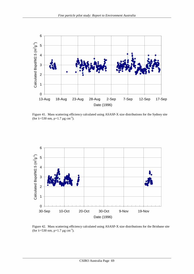
Fine particle pilot study: Report to Environment Australia
CSIRO Australia Page 69
0
1
2
3
4
5
6
13-Aug 18-Aug 23-Aug 28-Aug 2-Sep 7-Sep 12-Sep 17-Sep
Date (1996)
Cal
cula
ted
Bsp
d/M
2.5
(m2 g-1
)
Figure 41. Mass scattering efficiency calculated using ASASP-X size distributions for the Sydney site(for λ=530 nm, ρ=1.7 µg cm-3).
0
1
2
3
4
5
6
30-Sep 10-Oct 20-Oct 30-Oct 9-Nov 19-Nov
Date (1996)
Cal
cula
ted
Bsp
d/M
2.5
(m2 g-1
)
Figure 42. Mass scattering efficiency calculated using ASASP-X size distributions for the Brisbane site(for λ=530 nm, ρ=1.7 µg cm-3).

Fine particle pilot study: Report to Environment Australia
CSIRO Australia Page 70
0
1
2
3
4
5
6
2-Apr 7-Apr 12-Apr 17-Apr 22-Apr 27-Apr
Date (1997)
Cal
cula
ted
Bsp
d/M
2.5
(m2 g-1
)
Figure 43. Mass scattering efficiency calculated using ASASP-X size distributions for the Melbourne site(for λ=530 nm, ρ=1.7 µg cm-3).
0
1
2
3
4
5
6
30-Apr 5-May 10-May 15-May 20-May 25-May 30-May 4-Jun 9-Jun
Date (1997)
Cal
cula
ted
Bsp
d/M
2.5
(m2 g-1
)
Figure 44. Mass scattering efficiency calculated using ASASP-X size distributions for the Canberra site(for λ=530 nm, ρ=1.7 µg cm-3).

Fine particle pilot study: Report to Environment Australia
CSIRO Australia Page 71
0
1
2
3
4
5
6
9-Jun 19-Jun 29-Jun 9-Jul 19-Jul 29-Jul
Date (1997)
Cal
cula
ted
Bsp
d/M
2.5
(m2 g-1
)
Figure 45. Mass scattering efficiency calculated using ASASP-X size distributions for the Launceston site(for λ=530 nm, ρ=1.7 µg cm-3).
0
1
2
3
4
5
6
1-Aug 6-Aug 11-Aug 16-Aug 21-Aug 26-Aug
Date (1997)
Cal
cula
ted
Bsp
d/M
2.5
(m2 g-1
)
Figure 46. Mass scattering efficiency calculated using ASASP-X size distributions for the Adelaide site(for λ=530 nm, ρ=1.7 µg cm-3).

Fine particle pilot study: Report to Environment Australia
CSIRO Australia Page 72
For locations where large nocturnal loadings of smoke were observed, in particularCanberra and Launceston, corresponding mass scattering efficiencies based on particle sizeapproach a value of 5 m2 g-1 during the night. The values reduce to around 2.5 to 3 m2 g-1
during the day when particle loadings reduce with day-time decrease in the smoke source andincreased ventilation due to the daytime increase in vertical mixing.
For locations more dominated by vehicle sources, e.g. the Adelaide and Melbournesites, calculated mass scattering efficiencies are typically around 2.5 to 3.5 m2 g-1. Thedifference in mass scattering efficiency by a factor of two compared with Launceston andCanberra is due solely to local size distribution (i.e. aerosol source-type) differences. It pointsto the need for care in use of scattering data to infer fine mass in the absence of other aerosoldata. Errors of a factor of two or more in inferred mass would be possible, based on theseAFP Study data.
8.4 State/Territory Agencies: Instrument Comparison
One significant motivation for this study was a desire to investigate the relativeperformance of a variety of aerosol measurement instruments previously employed in Australiain both monitoring and research activities in the different jurisdictions. Such a broad-scaleassessment has not been undertaken previously in this country, but it is noteworthy that wheresuch instrument comparisons have been undertaken elsewhere using ambient aerosol,differences in performance between co-located measurement systems have often been found tobe significantly larger than would be expected based on the performance of the individualsystems under ideal (or laboratory test) conditions [e.g. see discussion included in Chow,1995]. The case of the TEOM discussed in the previous section illustrates this point well.
Protocols for assessment of aerosol system performance have been developed, mostnotably by the US EPA, which defines a given measurement system meeting a tightly specifiedprotocol as being a Federal Reference Method. Additional protocols that are met by non-reference methods allow classification of alternate measurements methods/systems asEquivalent Methods. For example the TEOM 1400 and 1400a series instruments areregistered as an Equivalent Method for PM10 determination. Although PM2.5 and even PM1measurements now figure significantly in both technical and policy debates concerning theatmospheric aerosol [e.g. Chow, 1995; Vedal, 1997], the regulations focus almost exclusivelyon PM10 in terms of performance specifications. A convenient and thorough overview of therecent US position is provided by Chow [1995].
In Australia the situation is somewhat less developed. The two Australian Standardsrelevant to the AFP Study are AS 3580.9.6-1990 and AS 3580.9.7-1990, defining the methodsand performance requirements for PM10 determination by manual gravimetric analysis of HighVolume sampler filters and Dichotomous sampler filters, respectively. These AustralianStandards derive heavily from the relevant US literature.
The resources and time available to the AFP Study precluded carrying out performanceevaluations in the form detailed in the US EPA Methods or Australian Standards: it was simplyimpossible to meet the defined hardware requirements (co-location of three samplers of eachtype), or sampling requirements (≥15 twenty-four hour samples per site, with a minimum offive samples having PM10 greater than 50 µg m-3). Therefore an alternative, pragmaticapproach was adopted in the AFP Study.
A key element in this was the use of a single “reference package” of aerosolmeasurement systems that would be deployed sequentially in parallel with local authoritymeasurement systems in six different state/territory locations across the country. The aim was
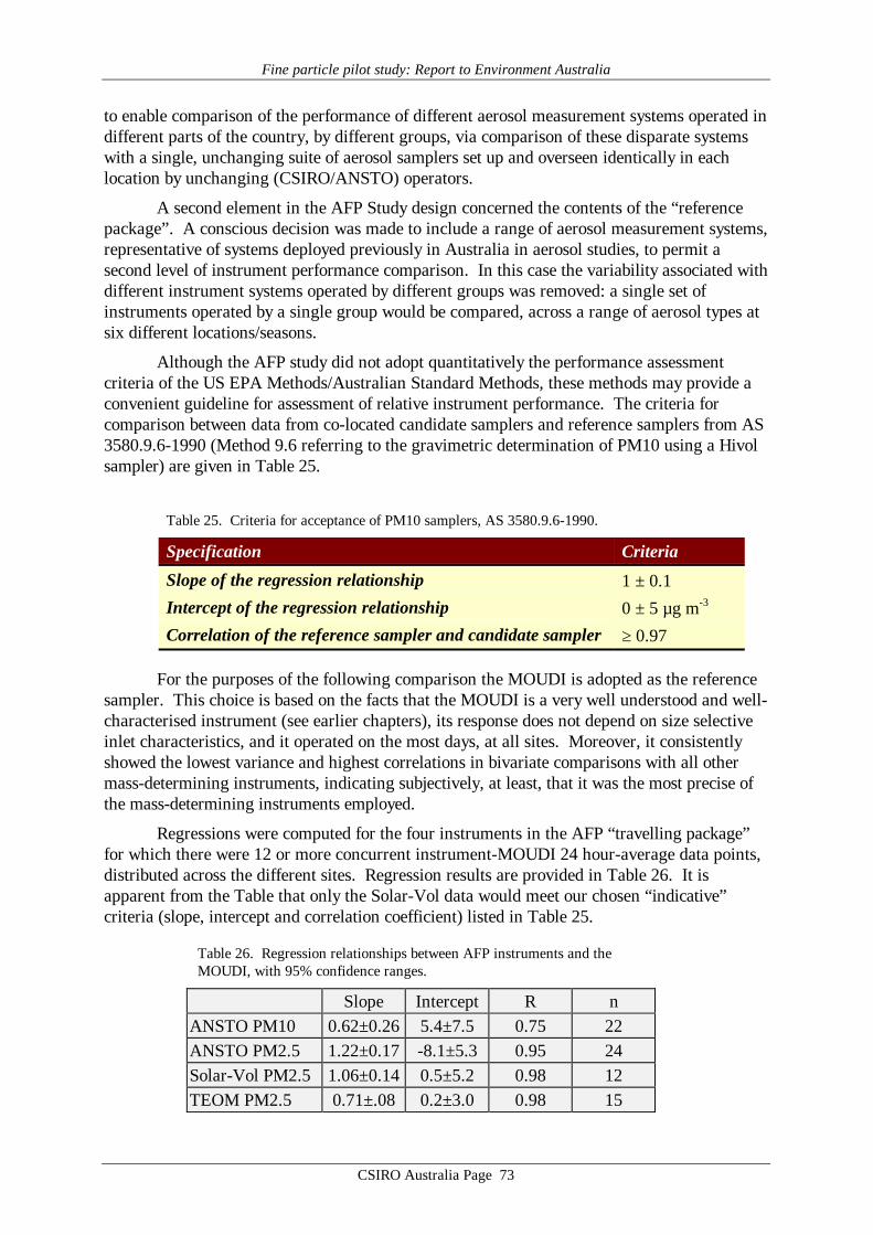
Fine particle pilot study: Report to Environment Australia
CSIRO Australia Page 73
to enable comparison of the performance of different aerosol measurement systems operated indifferent parts of the country, by different groups, via comparison of these disparate systemswith a single, unchanging suite of aerosol samplers set up and overseen identically in eachlocation by unchanging (CSIRO/ANSTO) operators.
A second element in the AFP Study design concerned the contents of the “referencepackage”. A conscious decision was made to include a range of aerosol measurement systems,representative of systems deployed previously in Australia in aerosol studies, to permit asecond level of instrument performance comparison. In this case the variability associated withdifferent instrument systems operated by different groups was removed: a single set ofinstruments operated by a single group would be compared, across a range of aerosol types atsix different locations/seasons.
Although the AFP study did not adopt quantitatively the performance assessmentcriteria of the US EPA Methods/Australian Standard Methods, these methods may provide aconvenient guideline for assessment of relative instrument performance. The criteria forcomparison between data from co-located candidate samplers and reference samplers from AS3580.9.6-1990 (Method 9.6 referring to the gravimetric determination of PM10 using a Hivolsampler) are given in Table 25.
Table 25. Criteria for acceptance of PM10 samplers, AS 3580.9.6-1990.
Specification Criteria
Slope of the regression relationship 1 ± 0.1Intercept of the regression relationship 0 ± 5 µg m-3
Correlation of the reference sampler and candidate sampler ≥ 0.97
For the purposes of the following comparison the MOUDI is adopted as the referencesampler. This choice is based on the facts that the MOUDI is a very well understood and well-characterised instrument (see earlier chapters), its response does not depend on size selectiveinlet characteristics, and it operated on the most days, at all sites. Moreover, it consistentlyshowed the lowest variance and highest correlations in bivariate comparisons with all othermass-determining instruments, indicating subjectively, at least, that it was the most precise ofthe mass-determining instruments employed.
Regressions were computed for the four instruments in the AFP “travelling package”for which there were 12 or more concurrent instrument-MOUDI 24 hour-average data points,distributed across the different sites. Regression results are provided in Table 26. It isapparent from the Table that only the Solar-Vol data would meet our chosen “indicative”criteria (slope, intercept and correlation coefficient) listed in Table 25.
Table 26. Regression relationships between AFP instruments and theMOUDI, with 95% confidence ranges.
Slope Intercept R nANSTO PM10 0.62±0.26 5.4±7.5 0.75 22ANSTO PM2.5 1.22±0.17 -8.1±5.3 0.95 24Solar-Vol PM2.5 1.06±0.14 0.5±5.2 0.98 12TEOM PM2.5 0.71±.08 0.2±3.0 0.98 15
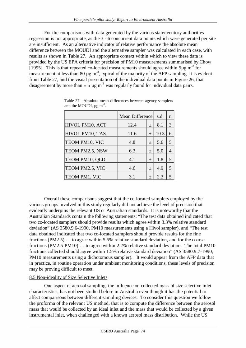
Fine particle pilot study: Report to Environment Australia
CSIRO Australia Page 74
For the comparisons with data generated by the various state/territory authoritiesregression is not appropriate, as the 3 - 6 concurrent data points which were generated per siteare insufficient. As an alternative indicator of relative performance the absolute meandifference between the MOUDI and the alternative sampler was calculated in each case, withresults as shown in Table 27. An appropriate context within which to view these data isprovided by the US EPA criteria for precision of PM10 measurements summarised by Chow[1995]. This is that repeated co-located measurements should agree within 5µg m-3 formeasurement at less than 80 µg m-3, typical of the majority of the AFP sampling. It is evidentfrom Table 27, and the visual presentation of the individual data points in Figure 26, thatdisagreement by more than ± 5 µg m-3 was regularly found for individual data pairs.
Table 27. Absolute mean differences between agency samplersand the MOUDI, µg m-3.
Mean Difference s.d. n
HIVOL PM10, ACT 12.4 ± 8.1 3
HIVOL PM10, TAS 11.6 ± 10.3 6
TEOM PM10, VIC 4.8 ± 5.6 5
TEOM PM2.5, NSW 6.3 ± 5.0 4
TEOM PM10, QLD 4.1 ± 1.8 5
TEOM PM2.5, VIC 4.6 ± 4.9 5
TEOM PM1, VIC 3.1 ± 2.3 5
Overall these comparisons suggest that the co-located samplers employed by thevarious groups involved in this study regularly did not achieve the level of precision thatevidently underpins the relevant US or Australian standards. It is noteworthy that theAustralian Standards contain the following statements: “The test data obtained indicated thattwo co-located samplers should provide results which agree within 3.3% relative standarddeviation” (AS 3580.9.6-1990, PM10 measurements using a Hivol sampler), and “The testdata obtained indicated that two co-located samplers should provide results for the finefractions (PM2.5) … .to agree within 5.5% relative standard deviation, and for the coarsefractions (PM2.5-PM10) … .to agree within 2.2% relative standard deviation. The total PM10fractions collected should agree within 1.5% relative standard deviation” (AS 3580.9.7-1990,PM10 measurements using a dichotomous sampler). It would appear from the AFP data thatin practice, in routine operation under ambient monitoring conditions, these levels of precisionmay be proving difficult to meet.
8.5 Non-ideality of Size Selective Inlets
One aspect of aerosol sampling, the influence on collected mass of size selective inletcharacteristics, has not been studied before in Australia even though it has the potential toaffect comparisons between different sampling devices. To consider this question we followthe proforma of the relevant US method, that is to compute the difference between the aerosolmass that would be collected by an ideal inlet and the mass that would be collected by a giveninstrumental inlet, when challenged with a known aerosol mass distribution. While the US
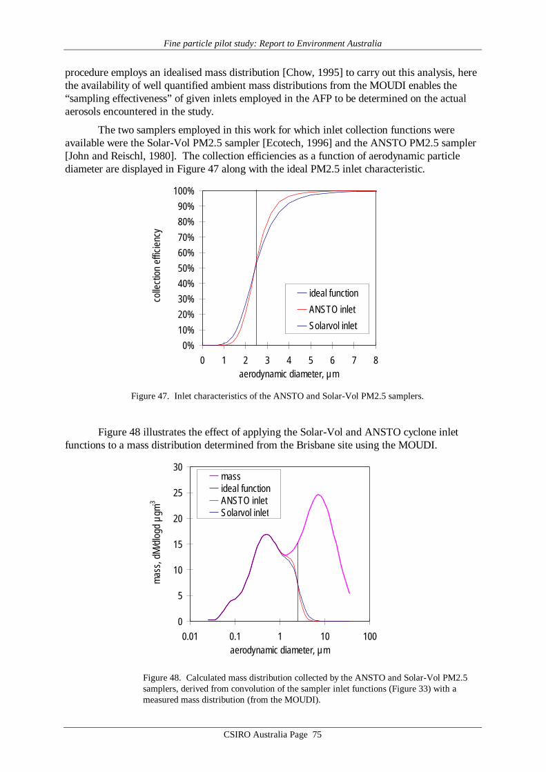
Fine particle pilot study: Report to Environment Australia
CSIRO Australia Page 75
procedure employs an idealised mass distribution [Chow, 1995] to carry out this analysis, herethe availability of well quantified ambient mass distributions from the MOUDI enables the“sampling effectiveness” of given inlets employed in the AFP to be determined on the actualaerosols encountered in the study.
The two samplers employed in this work for which inlet collection functions wereavailable were the Solar-Vol PM2.5 sampler [Ecotech, 1996] and the ANSTO PM2.5 sampler[John and Reischl, 1980]. The collection efficiencies as a function of aerodynamic particlediameter are displayed in Figure 47 along with the ideal PM2.5 inlet characteristic.
0%10%20%30%40%50%60%70%80%90%
100%
0 1 2 3 4 5 6 7 8aerodynamic diameter, µm
colle
ctio
n ef
ficie
ncy
ideal function
ANSTO inlet
Solarvol inlet
Figure 47. Inlet characteristics of the ANSTO and Solar-Vol PM2.5 samplers.
Figure 48 illustrates the effect of applying the Solar-Vol and ANSTO cyclone inletfunctions to a mass distribution determined from the Brisbane site using the MOUDI.
0
5
10
15
20
25
30
0.01 0.1 1 10 100aerodynamic diameter, µm
mas
s, d
M/d
logd
µgm
-3
massideal functionANSTO inletSolarvol inlet
Figure 48. Calculated mass distribution collected by the ANSTO and Solar-Vol PM2.5samplers, derived from convolution of the sampler inlet functions (Figure 33) with ameasured mass distribution (from the MOUDI).

Fine particle pilot study: Report to Environment Australia
CSIRO Australia Page 76
Application of the Solar-Vol and ANSTO inlet functions to a total of 28 MOUDI massdistributions taken across the six AFP sampling sites resulted in an average loss of PM2.5 massof 1.1% (standard deviation 1.5%) for the Solar-Vol, and 0.7% (standard deviation 1.4%) forthe ANSTO sampler. According to the US criterion summarised by Chow [1995] for PM10the effect of the inlet should be less than 10% in comparison with the ideal sampler. Both theSolar-Vol and the ANSTO sampler meet this requirement. It is pertinent to add that at thelevels of PM2.5 measured at all sites except Launceston, systematic discrepancies of order 1%computed here are too small to explain the much larger random discrepancies sometimesexceeding ±5 µg m-3, discussed in the previous section.
8.6 PM10/PM2.5/PM1 Mass Relationships
In the literature discussions of the possible effects of the atmospheric aerosol on humanhealth the question of causation is acknowledged by all sides to be vexed [e.g. Seaton et al.,1995; Vedal, 1997, NEPC, 1997; Wilson and Suh, 1997; see also multiple comments in J. Air& Waste Management, Vol. 47, 1997]. Variations in each of PM10, PM2.5 and PM1, as wellas individual components such as acid sulfate, organic compounds, and even non-mass-basedparameters such as “ultrafine” (or CN) number concentration have been proposed asparameters linked with adverse human health outcomes. The absence of clearly identifiablecausation in the face of published study results linking adverse heath effects with PM10 hascaused considerable difficulty in policy development both in the US [Vedal, 1997; Wilson andSuh, 1997], and in Australia where a PM2.5 ambient standard has been mooted but wasdiscarded in favour of PM10 [NEPC, 1997], perhaps at least partially on the basis that PM10may act adequately as a surrogate for PM2.5.
The MOUDI data obtained in the AFP Study provide an opportunity to investigate therelationships between the alternative mass-based parameters. A particular advantage of theMOUDI data is that the PM10, PM2.5 and PM1 values may all be derived from a singlemeasurement, thus avoiding errors introduced by differences in sampler performance that areunavoidable if different samplers are required for each PM measurement. As discussed inSection 7.2, PM10 contains at the large size end a significant component of refractorymaterial, produced by mechanical processes, including wind-blown soil dust (Figure 14) andsea-salt (Figure 15). PM2.5 and PM1 fractions contain less of this mechanically-producedaerosol, and relatively more of the products of combustion processes, such as vehicularemissions (Figure 12) and wood-burning (Figure 16), as well as gas-particle conversionproducts responsible for aerosol acidity (Figure 13). The details of how each size fractions isrepresented by these sources for each city are discussed also discussed in Section 7.2 and listedin Table 22.
Figures 49 - 51 show the bivariate relationships between the PM10 and PM2.5 sizefractions in the 24 hour mean MOUDI samples taken across all six AFP sites. Figures 52 – 54show the comparable plots for the PM2.5 and PM1 fractions.
The first three figures show that the MOUDI PM2.5 fraction of PM10 is wellcorrelated with PM10, however the PM10-PM2.5 fraction of PM10 is only weakly correlatedwith both PM10 and PM2.5 aerosol fractions. In the case of the PM2.5 and PM1 fractions ofthe aerosol (Figures 52 - 54) not only do these two fractions correlate well, but the PM2.5-PM1 fraction also correlates well with both PM2.5 and PM1.

Fine particle pilot study: Report to Environment Australia
CSIRO Australia Page 77
y = 1.09x + 7.33R2 = 0.98
0
20
40
60
80
100
120
0 20 40 60 80 100 120PM2.5, µgm-3
PM10
,µgm
-3
Figure 49. PM10 vs PM2.5, all AFP samples (24 hour mean values).
y = 0.10x + 6.02R2 = 0.35
0
5
10
15
20
0 50 100 150PM10, µg m-3
PM10
-PM
2.5,
µg m
-3
Figure 50. PM10-PM2.5 vs PM10, all AFP samples (24 hour mean values).
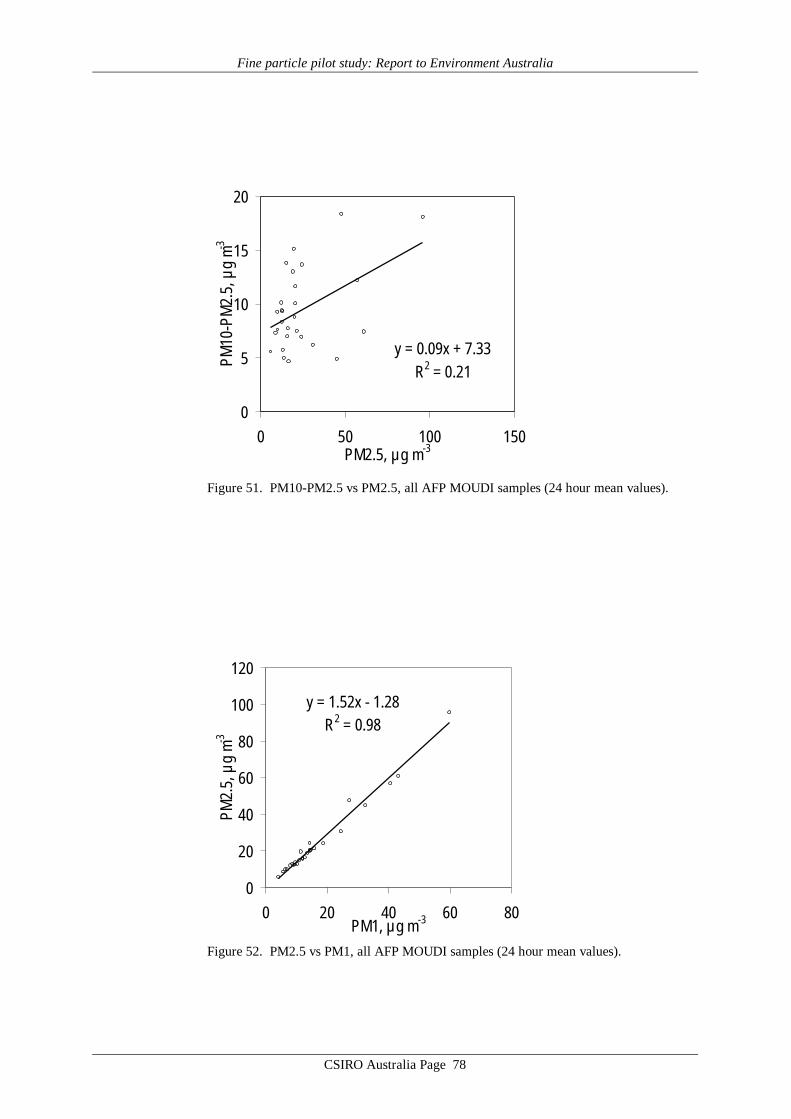
Fine particle pilot study: Report to Environment Australia
CSIRO Australia Page 78
y = 0.09x + 7.33R2 = 0.21
0
5
10
15
20
0 50 100 150PM2.5, µg m-3
PM10
-PM
2.5,
µg
m-3
Figure 51. PM10-PM2.5 vs PM2.5, all AFP MOUDI samples (24 hour mean values).
y = 1.52x - 1.28R2 = 0.98
0
20
40
60
80
100
120
0 20 40 60 80PM1, µg m-3
PM2.
5, µ
g m-3
Figure 52. PM2.5 vs PM1, all AFP MOUDI samples (24 hour mean values).

Fine particle pilot study: Report to Environment Australia
CSIRO Australia Page 79
y = 0.36x - 1.16R2 = 0.94
0
10
20
30
40
0 30 60 90 120PM2.5, µg m-3
PM2.
5-PM
1, µ
g m-3
Figure 53. PM2.5-PM1 vs PM2.5, all AFP MOUDI samples (24 hour mean values).
y = 0.52x - 1.28R2 = 0.85
0
10
20
30
40
0 20 40 60 80PM1, µg m-3
PM2.
5-PM
1, µ
g m-3
Figure 54. PM2.5-PM1 vs PM1, all AFP MOUDI samples (24 hour mean values).
These results suggest that in the AFP samples variability in PM10 is dominated byvariability in the PM2.5 fraction, rather than the PM10-PM2.5 fraction. If the results from thesix AFP sites apply to Australian environments generally, then it suggests the possibility thatstatistical associations between health outcomes and variance in PM10 in Australia may be dueto PM2.5, rather than the PM10-PM2.5 component of PM10. If such a hypothesis weretested and found to be sustained, this would provide an argument for an ambient aerosolstandard based on PM2.5 mass concentration rather than the current PM10 massconcentration.
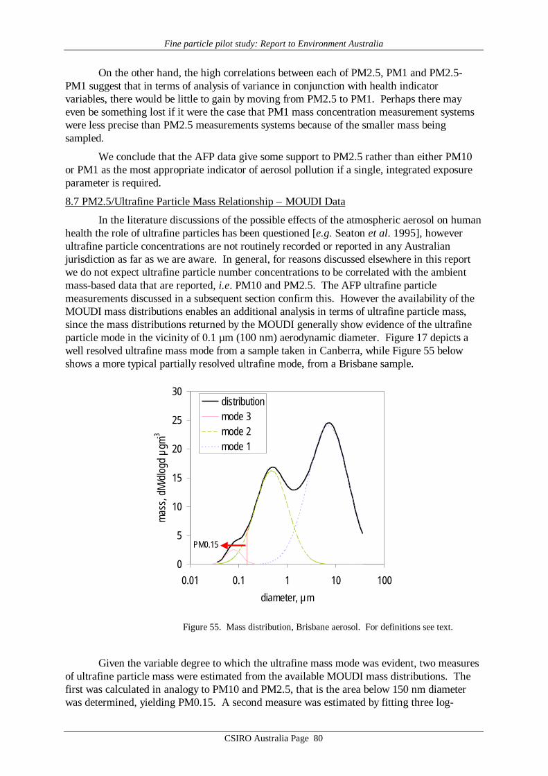
Fine particle pilot study: Report to Environment Australia
CSIRO Australia Page 80
On the other hand, the high correlations between each of PM2.5, PM1 and PM2.5-PM1 suggest that in terms of analysis of variance in conjunction with health indicatorvariables, there would be little to gain by moving from PM2.5 to PM1. Perhaps there mayeven be something lost if it were the case that PM1 mass concentration measurement systemswere less precise than PM2.5 measurements systems because of the smaller mass beingsampled.
We conclude that the AFP data give some support to PM2.5 rather than either PM10or PM1 as the most appropriate indicator of aerosol pollution if a single, integrated exposureparameter is required.
8.7 PM2.5/Ultrafine Particle Mass Relationship – MOUDI Data
In the literature discussions of the possible effects of the atmospheric aerosol on humanhealth the role of ultrafine particles has been questioned [e.g. Seaton et al. 1995], howeverultrafine particle concentrations are not routinely recorded or reported in any Australianjurisdiction as far as we are aware. In general, for reasons discussed elsewhere in this reportwe do not expect ultrafine particle number concentrations to be correlated with the ambientmass-based data that are reported, i.e. PM10 and PM2.5. The AFP ultrafine particlemeasurements discussed in a subsequent section confirm this. However the availability of theMOUDI mass distributions enables an additional analysis in terms of ultrafine particle mass,since the mass distributions returned by the MOUDI generally show evidence of the ultrafineparticle mode in the vicinity of 0.1 µm (100 nm) aerodynamic diameter. Figure 17 depicts awell resolved ultrafine mass mode from a sample taken in Canberra, while Figure 55 belowshows a more typical partially resolved ultrafine mode, from a Brisbane sample.
0
5
10
15
20
25
30
0.01 0.1 1 10 100
diameter, µm
mas
s, d
M/d
logd
µgm
-3
distributionmode 3mode 2mode 1
PM0.15
Figure 55. Mass distribution, Brisbane aerosol. For definitions see text.
Given the variable degree to which the ultrafine mass mode was evident, two measuresof ultrafine particle mass were estimated from the available MOUDI mass distributions. Thefirst was calculated in analogy to PM10 and PM2.5, that is the area below 150 nm diameterwas determined, yielding PM0.15. A second measure was estimated by fitting three log-

Fine particle pilot study: Report to Environment Australia
CSIRO Australia Page 81
normal distributions to each overall MOUDI mass distribution, allowing ultrafine particle massto be estimated as the area under the log-normal mode centred near 0.1 µm (Figure 55).
Correlations between both measures of ultrafine particle mass and both PM10 andPM2.5 were calculated, essentially addressing the question as to whether either of thesecommonly determined aerosol parameters also acted as a surrogate for ultrafine particle mass.All correlations were found to be weak, as illustrated by Figure 56 which shows thecomparison with PM2.5.
y = 0.034x + 1.759R2 = 0.500
y = 0.006x + 1.017R2 = 0.014
0
1
2
3
4
5
6
0 20 40 60 80 100 120
PM2.5, µg m-3
Ultra
fine
mas
s, µ
g m-3
PM0.15mode 3
Figure 56. Relationships between two measures ofultrafine particle mass and PM2.5
We conclude that the currently measured mass-based aerosol indicators PM10 andPM2.5 do not act effectively as surrogates for ultrafine particle mass in the AFP MOUDIsamples.
8.8 Aerosol Elemental Carbon
Elemental carbon (EC) is one individual aerosol component that makes up a significantpart of PM10 and PM2.5 aerosol mass. It is commonly measured in aerosolassessment/source apportionment studies. In urban air it is frequently used as one of severaltracers for automotive emissions, especially diesel emissions. It may also be used in theestimation of aerosol organic matter by difference (i.e. organic mass = total mass – EC –inorganic mass), so accurate measurement of aerosol EC levels is desirable.
However experience internationally has been that aerosol carbon determinations, bothfor EC and organic carbon (OC), are difficult to carry out with accuracy and precision.Comparisons between different co-located measurement systems often yield differences of afactor of two or more [e.g. Hering et al., 1990; Horvath, 1997; Heintzenberg et al., 1998].
Within the Australian context the possibility of such variation between measurementsystems is important, since previous aerosol assessment studies carried out in different parts ofthe country by different groups have yielded significantly different levels of EC content inPM2.5 aerosol. For example, the ASP Study carried out in NSW reported an average ECcontribution to PM2.5 mass of 23% [ERDC, 1995], whereas the Perth Haze Study [Gras,
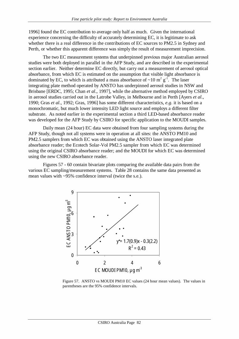
Fine particle pilot study: Report to Environment Australia
CSIRO Australia Page 82
1996] found the EC contribution to average only half as much. Given the internationalexperience concerning the difficulty of accurately determining EC, it is legitimate to askwhether there is a real difference in the contributions of EC sources to PM2.5 in Sydney andPerth, or whether this apparent difference was simply the result of measurement imprecision.
The two EC measurement systems that underpinned previous major Australian aerosolstudies were both deployed in parallel in the AFP Study, and are described in the experimentalsection earlier. Neither determine EC directly, but carry out a measurement of aerosol opticalabsorbance, from which EC is estimated on the assumption that visible light absorbance isdominated by EC, to which is attributed a mass absorbance of ~10 m2 g-1. The laserintegrating plate method operated by ANSTO has underpinned aerosol studies in NSW andBrisbane [ERDC, 1995; Chan et al., 1997], while the alternative method employed by CSIROin aerosol studies carried out in the Latrobe Valley, in Melbourne and in Perth [Ayers et al.,1990; Gras et al., 1992; Gras, 1996] has some different characteristics, e.g. it is based on amonochromatic, but much lower intensity LED light source and employs a different filtersubstrate. As noted earlier in the experimental section a third LED-based absorbance readerwas developed for the AFP Study by CSIRO for specific application to the MOUDI samples.
Daily mean (24 hour) EC data were obtained from four sampling systems during theAFP Study, though not all systems were in operation at all sites: the ANSTO PM10 andPM2.5 samplers from which EC was obtained using the ANSTO laser integrated plateabsorbance reader; the Ecotech Solar-Vol PM2.5 sampler from which EC was determinedusing the original CSIRO absorbance reader; and the MOUDI for which EC was determinedusing the new CSIRO absorbance reader.
Figures 57 - 60 contain bivariate plots comparing the available data pairs from thevarious EC sampling/measurement systems. Table 28 contains the same data presented asmean values with ~95% confidence interval (twice the s.e.).
y = 1.7(0.9)x - 0.3(2.2)R2 = 0.43
0
3
6
9
0 2 4 6EC MOUDI PM10, µg m-3
EC A
NSTO
PM
10, µ
g m-3
Figure 57. ANSTO vs MOUDI PM10 EC values (24 hour mean values). The values inparentheses are the 95% confidence intervals.

Fine particle pilot study: Report to Environment Australia
CSIRO Australia Page 83
y = 3.3(1.8)x - 1.4(4.0)R2 = 0.40
0
5
10
15
20
0 1 2 3 4 5EC MOUDI PM2.5, µg m-3
EC A
NSTO
PM
2.5,
µg
m-3
Figure 58. ANSTO vs MOUDI PM2.5 EC values (24 hour mean values) ). The values inparentheses are the 95% confidence intervals.
y = 1.6(1.1)x - 0.7(2.9)R2 = 0.67
0
2
4
6
8
0 2 4 6EC MOUDI PM2.5, µg m-3
EC S
olar
vol P
M2.
5, µ
g m-3
Figure 59. Solar-Vol vs MOUDI PM2.5 EC (24 hour mean values). The values inparentheses are the 95% confidence intervals.

Fine particle pilot study: Report to Environment Australia
CSIRO Australia Page 84
y = 2.0(1.4)x - 1.2(5.5)R2 = 0.71
0
4
8
12
16
0 2 4 6 8EC Solarvol PM2.5, µg m-3
EC A
NSTO
PM
2.5,
µg
m-3
Figure 60. ANSTO vs Solar-Vol PM2.5 EC (24 hour mean values). The values inparentheses are the 95% confidence intervals.
Table 28. Mean EC values (µg m-3) with ~95%confidence intervals. The slight differencesapparent for a given sampler in the differentcomparisons reflects the differing numbers of datapairs in each case.
PM10
MOUDI ANSTO
Mean 95% Mean 95%
2.2 ± 0.4 3.4 ± 1.1
PM2.5
MOUDI ANSTO
Mean 95% Mean 95%
2.0 ± 0.4 5.3 ± 2.1
MOUDI Solar-Vol
Mean 95% Mean 95%
2.4 ± 0.4 3.1 ± 0.8
Solar-Vol ANSTO
Mean 95% Mean 95%
3.5 ± 0.7 5.7 ± 1.7

Fine particle pilot study: Report to Environment Australia
CSIRO Australia Page 85
Two features of the data stand out. First, that the precision of the EC estimations,judged by the scatter in the plots, is considerably worse than that of the gravimetric massdeterminations presented and discussed earlier (Figures 20 - 24). Second, there is anindication of systematic variations in response of the systems, with the ANSTO samplersgenerally yielding higher EC estimates than the CSIRO samplers. For the PM2.5 data, theMOUDI results are lowest, the Solar-Vol results are on average higher, with the ANSTOPM2.5 EC data being the highest. These measurement systems not only employ differentoptical setups, but also quite different aerosol sample accumulations, which in turn meansdifferent optical geometries for the collected aerosol material. It is known that matrix effects(such as the contribution to extinction made by light scattering in the collected sample andfilter material) can vary significantly depending upon optical arrangement, filter type andsample loading [e.g. Horvath, 1997; Petzold et al., 1997; Heintzenberg et al., 1998]. In theAFP Study the ANSTO PM2.5 sampler collects aerosol at >7 times the flowrate used by theSolar-Vol, on a different filter type only one quarter the area of the Solar-Vol filter. As aresult, the ANSTO aerosol sample will have 30x physical thickness compared with the Solar-Vol. Yet another arrangement occurs with the MOUDI samples, as these are not uniformlydistributed over the collection surface but pile up in “spots” below each impaction jet. Theeffect of this on the light measurements is not well understood.
At this stage it is impossible to determine which of the systems return the mostaccurate estimate of aerosol EC loading. However it is clear that differences of factors of 2-3(differences of this order or more are evident in the plots) significantly affects the usefulness ofthe data. For example, a number of studies in which total aerosol carbon was determined byhigh temperature combustion of the aerosol material and determination of CO2 evolved, havedemonstrated “mass closure”. In other words, aerosol mass determined gravimetrically hasbeen shown to agree (within experimental uncertainty) with the independently determined sumof inorganic components plus total carbon, TC (EC plus OC).
Consistency of aerosol data is often assessed in terms of this idea of “mass closure”, ora test of whether total sample mass determined gravimetrically is accounted for by the sum ofthe major, independently determined aerosol components – organic matter, inorganic matterand elemental carbon. Good mass closure has been demonstrated in the USA, for example, bythe work of Malm et al. [1994] who used the same cyclone sampler and analysis procedures,including the same laser integrating plate methods (LIPM) as ANSTO. They have alsoperformed independent EC measurements finding good agreement with LIPM techniques. Atwo year study commencing in 1992 by ANSTO, at 25 sites across NSW, produced massclosure to (84±13)% which did not include 8% measured water vapour [ERDC 1995]. Morerecent work at selected sites in NSW for local Councils has produced mass closure to(92±9)% all using the LIPM techniques for EC measurements. If the EC measurements werehigh by a factor of two then the relatively good mass closure agreements would becomesignificantly worst for all these studies. The mass closure measured for the AFP study on allthe ANSTO PM2.5 samples using these methods was (96±26)%. The relatively high standarddeviation reflects the low numbers of samples and the fact that some samplers were runoutside their operating specifications on some days during the study period.
Figure 61 demonstrates another Australian example of this “mass closure”. Yetanother recent example is provided by the Perth Haze Study [see Figure 25 in Gras, 1996].

Fine particle pilot study: Report to Environment Australia
CSIRO Australia Page 86
0
10
20
30
0 10 20 30
~PM2.5 gravimetric, µg m-3
~PM
2.5
TC +
Inor
gani
cs, µ
g m-3
Figure 61. Mass closure from the Latrobe Valley Aerosol/VisibilityStudy (1986-1988): sum of inorganic and total carbon components vsgravimetric aerosol mass [Ayers et al., 1990].
Although reported in the studies quoted above, the confirmation that gravimetricallydetermined mass can be explained as the sum of inorganic plus organic components is nottrivial. The total carbon determinations are difficult, time consuming and costly, so it has beena practical choice for some purposes to not directly determine TC, instead relying on theassumption of mass closure to enable estimation of aerosol organic matter as the differencebetween gravimetric mass (GM), and the sum of inorganic components (IM) plus EC. In otherwords Estimated Organic Matter content (EOM) is determined as follows:
EOM = GM – IM – EC.
Clearly, large disparities in EC or IM would make such a procedure problematic,therefore calculation of EOM for the AFP samples constitutes a sensitive test of theconsistency of the GM, IM and EC data. Here we carry out such a consistency test,comparing EOM data calculated from different AFP samplers. We anticipate, in particular,that systematic differences in results from different EC measurement systems would flowthrough to the EOM calculation to yield systematic EM differences in EOM of the oppositesense. This was found to be the case, as illustrated Figure 62, which contrasts EOM datacalculated from the ANSTO PM2.5 EC data (highest EC results) with the MOUDI PM2.5 ECdata (lowest EC results).

Fine particle pilot study: Report to Environment Australia
CSIRO Australia Page 87
-5
0
5
10
15
0 10 20
1:1
y = 1.14(0.17)x - 9.3(4.4)R2 = 0.90
-20
0
20
40
60
80
100
0 50 100
EOM MOUDI PM2.5, µg m-3
EOM
ANS
TO P
M2.
5, µ
g m-3
Figure 62. EOM derived from the ANSTO PM2.5 sampler vs EOM fromthe MOUDI PM2.5 data (24 hour mean values).
At higher PM2.5 mass loadings the EOM values agree reasonably well, but at the morefrequently encountered lower levels, as shown in the inset, there is a very large systematic biastowards the MOUDI having much higher EOM, and little correlation – a consequence ofsubtracting off systematically lower EC values than for the ANSTO sampler. There is alsosome evidence in the fact that the ANSTO EOM values go to zero, and even negative, that theANSTO EC values may be systematically high for the lower mass samples.
As noted earlier it is not possible to do more here than to highlight the differencesbetween the different measurement systems. An obvious conclusion to be drawn from theseresults is that aerosol EC values from the various aerosol studies carried out previously inAustralia should be interpreted and compared with caution.
The same conclusion is almost certainly true of aerosol organic matter data. Forexample it may be that the above definition of EOM is not such a good one for low values ofEOM and other techniques such as the one described earlier in section 7.1, where the totalhydrogen and sulfur measurements are used, could be more appropriate. However thismethod also has certain underlying assumptions built into the data estimation procedure. Thuswhile the question of organic matter estimation in aerosol samples has not been considered indetail here, it would appear prudent to conclude for OC, as in the case of EC, that extantAustralian data should be interpreted and compared with caution.
Fine particle pilot study: Report to Environment Australia
CSIRO Australia Page 88
9. Conclusions and Recommendations
A comprehensive range of fine particle physical and chemical properties has beendetermined during one month at each of six sites in Eastern Australia (located in Sydney,Brisbane, Melbourne, Canberra, Launceston and Adelaide). The particle measurement systemsdeployed by CSIRO and ANSTO were operated in parallel with the routine particlemeasurements carried out by the relevant State/Territory agency, enabling an evaluation of thecomparability of data from the various measurement systems.
9.1 Comparability of Measurement Systems
At the fine particle levels encountered in the six locations studied, the variousmeasurements of aerosol mass concentration regularly differed by more than the expectedlevels of measurement system uncertainty. In routine operation, the levels of performance forco-located samplers implied in the Australian PM10 standards [AS 3580.9.6-1990/AS3580.9.9-1990] and relevant US standards [summarised by Chow, 1995] were not alwaysachieved.
The key source of variance between aerosol measurement systems appears to be theextent to which semi-volatile aerosol material is collected and determined. One component ofthis is atmospheric water, which may readily exchange with aerosol material sampled on filtersin response to change in humidity. Although this fact is well known and allowed for in thestandard (gravimetric) PM10 methods, tighter control of humidity during the gravimetricanalysis of filters appears desirable. In this regard, it is noteworthy that the least variancebetween gravimetric data pairs was achieved by the MOUDI (Micro-Orifice Uniform DepositImpactor) and Solar-Vol samplers: both were operated by the CSIRO group, which had thestrictest control of humidity during filter weighing.
A second component of semi-volatile aerosol material occurs in the organic fraction.In general, systematically lower PM2.5 and PM1 values were determined by TEOM (TaperedElement Oscillating Microbalance) measurement systems in comparison with the manual,gravimetric systems. The discrepancy was of order 30% between the CSIRO PM2.5 TEOMand the MOUDI in the AFP Study. The principal difference between these systems is that theTEOMs operate with the inlet air stream heated to well above ambient temperature (commonlyto 50ºC) whereas the manual gravimetric systems collect aerosol material at ambienttemperature. Evidence in the international literature supports the view that volatilisation ofsemi-volatile organic material in the heated inlet is a cause of systematically lower TEOM data.
Comparison of the two measurement systems used extensively to estimate aerosolelemental carbon (EC) content in previous Australian fine particle studies revealed a systematicdifference approaching a factor of two. Differences of this magnitude have been foundinternationally in comparisons between aerosol carbon measurement systems, underlining thedifficulties inherent in these measurements.
Taking into consideration all these findings we recommend that:
(1) a nationally coherent approach to particle measurement systems should be developed,incorporating performance standards for PM parameters that are amenable to validation ona regular basis (for example by comparison of operational instruments in routine use with asingle national “calibration” sampler operated by a single agency);

Fine particle pilot study: Report to Environment Australia
CSIRO Australia Page 89
(2) consideration should be given to seeking a common sampling system for particlemeasurements in all jurisdictions, to avoid differences between different sampler types anddifferent operational procedures;
(3) care should be exercised in the use of heating to achieve humidity control for measurementsystems such as the nephelometer or TEOM; where heating is used operationally theextent of loss of semi-volatile aerosol material should be assessed by comparison withmanual, gravimetric measurements undertaken at ambient temperature;
(4) consideration should be given to employing alternate methods of humidity control (drying)in Australian fine particle measurement systems;
(5) comparisons between absolute EC levels reported from previous Australian fine particlestudies should be made with caution; research should be undertaken to evaluate availablemethods of aerosol carbon measurement with a view to developing a single method ofmeasurement for aerosol carbon that is appropriate for Australian conditions.
9.2 Relationships Between PM10, PM2.5 and PM1
The MOUDI has been used in the AFP study to provide data on aerosol mass andchemical composition over the TSP, PM10, PM2.5 and PM1 aerosol fractions simultaneously,without the additional error that must intrude if these four parameters are measured by fourseparate instruments.
While PM10 and PM2.5 data show a strong structural relationship, variability in PM10was found to be dominated by variability in the PM2.5 fraction, rather than the PM10-PM2.5fraction. Thus, the statistical relationships noted between health outcomes and PM10 are mostlikely caused by the PM2.5 component of the size fraction, rather than the PM10-PM2.5fraction. This would appear to provide an argument for an ambient aerosol standard based onPM2.5 mass concentration rather than the current PM10 mass concentration. It suggests thatstronger relationships might be observed between PM2.5 and health outcomes, than arecurrently observed between PM10 and health outcomes, if more PM2.5 data were available,i.e. if PM2.5 data were regularly monitored and reported.
On the other hand, the high correlations between each of PM2.5, PM1 and PM2.5-PM1 suggest that in terms of analysis of variance in conjunction with health indicatorvariables, there would be little to gain by moving from PM2.5 to PM1.
Therefore, we recommend that:
(6) PM2.5 measurements should be undertaken routinely in Australia (initially in conjunctionwith existing PM10 measurements so as to provide a quantitative basis for determiningwhich is the better indicator of health effects of atmospheric particles);
(7) given high correlations found between PM1, PM2.5-PM1 and PM2.5, PM1 measurementsoffer no clear advantage over PM2.5 measurements as a mass-based indicator of potentialhealth effects of ambient particles.
9.3 Continuous Particle Measurement Systems: Nephelometer, TEOM, Ultrafine ParticleMeasurement Systems
The advantages of a continuous monitoring systems compared with 24 hour averagesampling on a 6 day cycle should be self-evident. Where high particle loadings occur on anevent basis, as in most Australian cities, this avoids the 5 in 6 probability of missing events,provides greater insights into physical processes, opens the prospects for examining laggedparticle-health relationships (over varying lag times) and allows much better statistics for
Fine particle pilot study: Report to Environment Australia
CSIRO Australia Page 90
health determinations where statistics are usually severely limited. However any measurementsystem has limitations as well as advantages, as noted above in the case of the TEOM.
Use of nephelometers to determine aerosol scattering coefficient (bspd) at multiple sitesin a number of Australian locales has a long history, going back as much as two decades.Although scattering coefficient as determined by a nephelometer is an integral property of theaerosol size distribution, the physics of the interaction between aerosol particles and visibleradiation is weighted towards particles in the sub-micrometre size range. Within the context ofan emerging focus internationally on the PM2.5 aerosol fraction, it is relevant to consider thepossibility that the extensive historical records of bspd might provide a surrogate historicalrecord for PM2.5, because this latter mass-based integral measure tends also to be dominatedby a mode in the mass distribution at diameters below 1 µm.
In the AFP Study we have confirmed that linear relationships can be found between bspd
(measured by nephelometer) and PM2.5 (measured by TEOM) in each city studied. Howeverdifferences in the scattering-mass relationships were identified, caused by site-specific aerosol(size distribution) properties. Thus if bspd were to be used as a surrogate historical record forPM2.5 the slope of the relationship would have to be determined for each site. An additionalcomplication is that at any given site this relationship may vary with season (not investigated inthe AFP study), so clearly caution would be required in any project aimed at harmonising thehistorical bspd data records with new and ongoing PM2.5 records. Other complicating mattersare the significant dependence of nephelometer output on humidity, and the strong implicationfrom the TEOM results that humidity reduction by heating, often used for nephelometers aswell as for the TEOM, may not be appropriate.
Ultrafine particle number concentration is also readily amenable to continuousmeasurement: such measurements were included in the AFP Study. The AFP study data showthat ultrafine particle number concentrations do not correlate with the ambient mass-baseddata normally reported, i.e. PM10 and PM2.5, nor with measures of ultrafine particle massderived from MOUDI data (i.e. estimates of PM0.15). We conclude that mass-based integralproperties of the aerosol do not provide surrogates for ultrafine particle number concentration.
Taking into consideration these findings we recommend that:
(8) a rigorous determination of the relationship between bspd and PM2.5 must be carried out ateach locality (over at least one complete annual cycle) where historical bspd data are to beused as a surrogate for fine mass data.
(9) ultrafine particle number concentrations cannot be inferred from mass-based aerosolmeasurements so must be determined directly using independent ultrafine particle (orcondensation nucleus) measurement systems.
9.4 Gaps in Knowledge
The AFP study has highlighted a number of areas where further understanding isrequired to underpin sound policy development. The most important lack of knowledgeconcerns semi-volatile aerosol material. A related issue, given the probable role of organicmaterial as a major fraction of the semi-volatile aerosol material, and the possible role of toxicorganic constituents in health effects, is a lack of certainty about the amount and types ofcarbonaceous material in the aerosol. In this regard we recommend that:
(10) studies be undertaken to characterise the semi-volatile component of aerosol material inthe major urban airsheds in Australia, in terms of its contribution to PM10 and PM2.5mass loading, its composition, sources, and variability with location and season;

Fine particle pilot study: Report to Environment Australia
CSIRO Australia Page 91
(11) uniform methods be developed and agreed between jurisdictions for the determination ofcarbonaceous aerosol material, in particular the components elemental carbon (EC) andorganic carbon (OC).
Discussions between the AFP Study team and representatives of the variousState/Territory agencies assisting with the measurement program suggest that a number ofaspects of fine particle monitoring and assessment may have been the subject of in-houseinvestigations carried out by some of these agencies. Useful information may have beengenerated, but remains not widely known or available. Therefore we recommend that:
(12) agencies be encouraged to make available to a central database, located in EnvironmentAustralia, copies of all published and unpublished work in their possession related toaerosol monitoring and assessment in Australia.
Finally, taking into consideration all the foregoing comments we recommend that:
(13) given the current uncertainty world-wide over the implications for human health ofexposure to fine particles, the uncertainty over choice of ambient indicator for fineparticles, the disparity of approaches taken to date by different agencies within Australia,and the evident differences between results from different measurements systems employedin the AFP Study, a national conference on fine particle monitoring and assessment shouldbe held. The aim would be to bring together the relevant regulatory agencies and researchinstitutions to seek a consensus on the development of a nationally uniform approach tofine particle monitoring and assessment within Australia.
Fine particle pilot study: Report to Environment Australia
CSIRO Australia Page 92
10. Acknowledgments
The AFP Study involved the co-operation of a large number of individuals. We wouldlike to thank several people for their help in obtaining access to the measurement sites,including Steve McPhail and George Richmond (EPA, NSW), David Wainwright (DoE,QLD), Trevor Bardsley and Cathy Wilson (EPA, VIC), Tony Hodgson (Environment, ACT)and Wayne Riley (ACT Analytical Laboratories), Frank Carnovale and Frank Cattel (DoE,TAS) and Bill Piesse (Launceston City Council), Rob Mitchell (EPA, SA) and the St GeorgeSchool, Therbaton.
The AFP research team gratefully acknowledges all the State and Territory Authoritypersonnel who assisted with field work, including Phil Kingston, Brendan Finn and BrianHaynes (DoE, QLD), Ian Fox and Kerry Boulder (ACT Analytical Laboratories) and RobertTrimble (DoE, TAS). We would also like to thank Neville Clark (Flinders University) for hishelp in the field.
Paul Selleck, Jenny Powell, Kate Boast and Tom Firestone (CSIRO) and EduardStelcer (ANSTO) are gratefully thanked for the contributions to the analysis of samples anddata. Rob Gillett, Mark Hibberd and Andrew Larkin are thanked for valuable discussons.

Fine particle pilot study: Report to Environment Australia
CSIRO Australia Page 93
11. References
Allen G., C. Sioutas, P. Koutrakis, R. Reiss, F.W. Lurmann and P.T. Roberts [1997],Evaluation of the TEOM method for measurement of ambient particulate mass in urban areas,J. Air Waste Management Assoc., 47, 682-689.
AS3580.9.6 [1990], Australian Standard methods for sampling and analysis of ambient air.Method 9.6: Determination of suspended particulate matter-PM10 high volume sampler withsize-selective inlet-Gravimetric method. Standards Australia, North Sydney, 11p.
AS3580.9.7 [1990], Australian Standard methods for sampling and analysis of ambient air.Method 9.6: Determination of suspended particulate matter-PM10 dichotomous sampler -Gravimetric method. Standards Australia, North Sydney, 11p.
Ayers G.P., E.K. Bigg, D.E. Turvey and M.J. Manton [1981], Urban influence oncondensation nuclei over a continent, Atmos. Environ., 16, 951-954.
Ayers G.P., Gras J.L., Gillett R.W. and Bentley S.T. [1990], The Latrobe ValleyAerosol/Visibility Study : a summary of results, Clean Air [Aust.], 24, 18 - 26.
Brook J. R., T. F. Dann and R. T. Burnett [1997], The relationship among TSP, PM10,PM2.5 and inorganic constituents of atmospheric particulate matter at multiple Canadianlocations, J. Air Waste Management Assoc., 47, 2-19.
Chan Y.C., R. W. Simpson, G. H. Mactainsh, P. D. Vowles, D. D. Cohen and G. M. Bailey[1997], Characterisation of chemical species in PM2.5 and PM10 aerosols in Brisbane,Australia, Atmos. Environ., 31, 3773-3785.
Chow J. C. [1995], Measurement methods to determine compliance with ambient air qualitystandards for suspended particles, J. Air Waste Management Assoc., 45, 320-382.
Ecotech [1996], Solar-Vol 1100 Particulate Sampler for PM10, PM2.5, TSP-ReferenceManual, Ecotech Pty Ltd, Blackburn, Australia, pp 26.
ERDC [1995], Contributions of fuel combustion pollution by airborne particles in urban andnon-urban environments. Report no. ERDC 259. Energy Research and DevelopmentCorporation, Canberra, Australia.
Gras J.L., R.W. Gillett, S.T. Bentley, G.P. Ayers and T. Firestone [1992], CSIRO-EPAMelbourne Aerosol Study, Final Report to EPA of Victoria.
Gras J.L. [1996] The Perth Haze Study. Report to the Department of EnvironmentalProtection of Western Australia, CSIRO.
Heintzenberg, J., R. J. Charlson, A. D. Clarke, C. Liousse, V. Ramaswamy, K. P. Shine, M.Wendisch and G. Helas [1998], Measurements and modelling of aerosol single-scatteringalbedo: Progress, problems and prospects, Bietr. Phys. Atmosph., 70, 249-263.
Hering S.V. et al. [1990], Comparison of sampling methods for carbonaceous aerosols inambient air, Aerosol Sci. and Technol., 12, 200-213.
Horvath H. [1997], Experimental calibration for aerosol light absorption measurement usingthe integrating plate method – summary of data, Aerosol Sci., 28, 1149-1161.
John W. and G. Reischl [1980], A cyclone for size-selective sampling of ambient air, J. AirPoll. Control Assoc., 30, 872-877.
Fine particle pilot study: Report to Environment Australia
CSIRO Australia Page 94
Lin C. I., M. Baker and R. C. Charlson [1973], Absorption coefficient of atmosphericparticles, Appl. Optics, 12, 1357-1363.
Malm C. W., J. F. Sisler, D. Huffman, R.A. Eldred and T.A. Cahill, [1994], Spatial andseasonal trends in particulate concentration and optical extinction in the United States, J.Geophys. Research, 99, 1347-1370.
Manton M.J. and G.P. Ayers [1982], The evolution of an aerosol plume from a town,Boundary Layer Met., 22, 171-181.
Marple V. A., K. L. Rubow and S. M. Behm [1991], A microorifice uniform deposit impactor[MOUDI]: Description, calibration and use, Aerosol Sci. and Technol., 14, 434-446.
Meyer M., J. Lijek and D. Ono [1992], Continuous PM10 measurements in a woodsmokeenvironment, PM10 Standards and Nontraditional Particulate Source Controls, J. C. Chowand D. M. Ono, Eds , Air Waste Management Assoc., TR-22, Vol 1 pp24-38.
Meyer M. and E. G. Rupprecht [1997], Particulate matter sampling methods: The importanceof standardisation, J. Aerosol Sci., 27, supp 1, S349-S350.
NEPC [1997], Towards a National Environment Protection Measure for Ambient Air Quality,National Environment Protection Council paper on ambient air quality.
Petzold A., C. Kopp and R. Neissner [1997], The dependence of the specific attenuationcross-section on black carbon mass fraction and particle size, Atmos. Environ., 31, 661-672.
RWTÜV [1994], Performance testing of the Rupprecht and Patashnick TEOM Series 1400aAmbient Particulate Monitor, Report to R&P from RWTÜV Anlagentechnik GmbH, Essen,Germany.
Seaton A., W. MacNee, K. Donaldson and D. Godden [1995], Particulate air pollution andacute health effects, Lancet, 345, 176-178.
Twomey S. A. and R. A. Zalabsky [1981], Mulitifilter technique for examination of the sizedistribution of the natural aerosol in the submicrometer range, Environmental Sci. Tech., 15,177-184.
Vedal S. [1997], Ambient particles and health: the lines that divide, J. Air Waste ManagementAssoc., 47, 551-581.
Wilson W. E. and H. H. Suh [1997], Fine particles and coarse particles: concentrationrelationship relevant to epidemiologic studies, J. Air Waste Management Assoc., 47, 1238-1249.
Winklmayr W., H-C, Wang and W. John [1990], Adaptation of the Twomey algorithm to theinversion of cascade impactor data, Aerosol Sci. Tech., 13, 322-331.
Working Party [1996], Report into Air Pollution Environmental Health and RespiratoryDiseases, Launceston and Upper Tamar Valley, Tasmanian 1991-1994, by the Air pollutionEnvironmental Health and Respiratory Diseases Working Party, published by Launceston CityCouncil.
Fine particle pilot study: Report to Environment Australia
CSIRO Australia Page 95
12. Glossary of selected terms
Term Meaning
Aerodynamic diameter defined property of any given atmospheric particle: the diameter of aspherical particle of density 1 g cm-3 that would have the sameaerodynamic behaviour as the given particle [Chow, 1995]
Aerosol generic term for a suspension of liquid or solid droplets/particles in afluid; the atmospheric aerosol consist of particles ranging in sizefrom molecular clusters (≤1 nm in diameter) to large cloud anddrizzle drops (~100 µm in diameter)
ASASP-X Particle Measuring Systems Inc. (PMS) active-cavity-laser particlesize spectrometer that uses light scatter in an open-cavity lasersystem to size individual particles over the diameter range of 100 nmto 3 µm (nominal) into 60 size channels (in four overlapping ranges)
bsp aerosol light scattering coefficient at ambient humidity
bspd aerosol light scattering coefficient for dry particles
babs aerosol light absorption coefficient
CN Condensation Nuclei; synonymous with the older term Aitkennuclei; effectively equivalent to the total number concentration ofatmospheric particles larger than the condensation nucleus counterminimum particle size threshold, typically ~3 nm particle diameter
CCN Cloud Condensation Nuclei; the subset of CN that act as centres forcloud droplet nucleation at the small supersaturations (typically 0.1 -1%) encountered in natural clouds; usually consists of particlescontaining soluble salts with diameter greater than about 10 – 50 nm
coarse particles old term mostly used by aerosol physicists to denote atmosphericparticles larger than about 1 µm in diameter
cut-point usually specified as 50% cut-point, or the aerodynamic particlediameter at which the sampling efficiency falls to 50%; i.e. thediameter at which an aerosol sampling device collects 50% ofincoming particles and transmits 50% of incoming particles
DMA Differential Mobility Analyser determine the mobility of an particlewhich is dependent on the size of the particle. In this study whenattached to a CN or UCN counter particle size distributions in therange 15 nm - 300 nm could be determined
EC Elemental Carbon
EOM Estimated Organic Matter (EOM) is determined as follows:
EOM=GM-IM-EC

Fine particle pilot study: Report to Environment Australia
CSIRO Australia Page 96
Term Meaning
fine particles old term mostly used by aerosol physicists to denote atmosphericparticles smaller than about 1 µm in diameter
GM Gravimetric Mass
IC Ion Chromatography; a method of analysis applicable to aqueousionic species; sensitive method applied to aerosol samples after thesamples are dissolved in high purity water
IM Inorganic Mass calculated (after Brook et al. 1997):IM=H++Na++1.41K++NH4
++1.63Ca2++Mg2++Cl-+NO3-+NO2
-+SO42-
+PO43+Pb+Br+1.79V+2.2Al+1.24Zn+2.5Si+1.58Fe+1.94Ti+Cr+
Mn+Co+Ni+Cu
M2.5 mass concentrations calculated from ASASP-X size distributions forparticle diameter less than 2.5 µm and an assumed density of 1.7 gcm-3
MOUDI Micro Orifice Uniform Deposit Impactor: aerosol sampling deviceused in this study to determine aerosol mass-size distribution overthe range ~0.05 - 20 µm in diameter [Marple et al., 1991]
nephelometer device used to measure bsp in real-time; based on illuminating alength of ambient air with a strong collimated light source in thevisible region, and collecting off-axis scattered light with a sensitivephotomultiplier/amplifier
particles generic term; widely understood common meaning; often usedinterchangeably with “aerosol”, as in “atmospheric particles” and“atmospheric aerosol”
particulates variation of the word “particles” usually applied in the regulatory or“air quality” communities, infrequently used by aerosol physicists; aterm to be avoided as a useless gloss
PIXE Proton Induced X-ray Emission; a method of elemental analysisbased on exciting a sample with a high energy proton beam andcollecting the emitted x-rays, for which specific x-ray energies areunique to each element; useful for elements above an atomic numberof 13
PM10 the subset of atmospheric particles having aerodynamic diametersless than 10 µm
PM2.5 the subset of atmospheric particles having aerodynamic diametersless than 2.5 µm
PM1 the subset of atmospheric particles having aerodynamic diametersless than 1 µm
STP Standard Temperature and Pressure: standard gas (atmospheric)conditions defined to be 273.15 Kelvin and 101.3 hPa

Fine particle pilot study: Report to Environment Australia
CSIRO Australia Page 97
Term Meaning
TEOM Tapered Element Oscillating Microbalance; device used todetermine real-time aerosol mass concentrations; use of differentinlets enables measurement to represent any one of TSP, PM10,PM2.5 or PM1; based on collecting aerosol on a tapered quartzelement, the oscillation frequency of which depends sensitively uponcollected aerosol mass
TSP Total Suspended Particle mass; mass concentration of particles of allsizes; usually expressed in units of µg m-3 at STP
UCN Ultrafine Condensation Nuclei (see ultrafine particles)
ultrafine particles new term entering scientific usage in the 1990’s referring to particlesin the aerodynamic diameter range from ~2nm to ~100 – 200 nm