Cheikh Ndour Simplice Dossou Gbété Abstract arXiv:1202

Classification Approach based on Association Rules mining forUnbalanced data

Cheikh Ndour1,2,3 & Aliou Diop1 & Simplice Dossou Gbété2

1 Laboratoire d’Etudes et de Recherche en Statistiques et Développement (LERSTAD), Unversité Gaston Berger,Saint-Louis, Sénégal2 Laboratoire de Mathématiques et de leurs Applications (LMA), UMR CNRS 5142, Université de Pau et desPays de L’Adour, Pau, France3 Institut de Santé Publique, d’Epidémiologie et de Développement (ISPED), INSERM U897, Université deBordeaux, Bordeaux, France

Abstract

This paper deals with the binary classification task when the target class has the lower prob-ability of occurrence. In such situation, it is not possible to build a powerful classifier by usingstandard methods such as logistic regression, classification tree, discriminant analysis, etc. Toovercome this short-coming of these methods which yield classifiers with low sensibility, wetackled the classification problem here through an approach based on the association rules learn-ing. This approach has the advantage of allowing the identification of the patterns that are wellcorrelated with the target class. Association rules learning is a well known method in the areaof data-mining. It is used when dealing with large database for unsupervised discovery of localpatterns that expresses hidden relationships between input variables. In considering associationrules from a supervised learning point of view, a relevant set of weak classifiers is obtained fromwhich one derives a classifier that performs well.

1 Introduction

This paper deals with the binary classification task when the target class has the lower probabilityof occurrence. In such situation, standard methods such as logistic regression [20], classificationtree, discriminant analysis, etc. do not make it possible to build an effective classification function[18]. They tend to focus on the prevalent class and to ignore the target class. Several works weredevoted on this subject, even in the recent past, as well as from the conventional statistical viewpointas such that of machine learning. Some works among them will consider the improvement of theregression models’ fitting to produce a classification function with a small prediction bias withoutloosing interesting features of the standard methods as the ability to evaluate the contribution of eachcovariate in the variations of target class probability (regression methods) or the identification of thepattern correlated with the target class(tree method). Alternative approaches consist in aggregationtechniques like boosting and bagging [12] which combine multiple classification functions with largeindividual error rate to produce a new classification function with smaller error rate [4].

Our aims is to propose a statistical learning method that provides an effective classifier and allowsto identify relevant patterns correlated with the target class. To achieve this goal we took the routetoward the association rules learning which is a well known method in the area of data mining. Itis used when dealing with large database for unsupervised discovery of local-patterns that expresshidden and potential valuable relationships between feature variables. In considering associationrules from a supervised statistical learning viewpoint, a relevant set of weak classifiers is obtainedfrom which one derives a classification function that performs well. Such an approach is not actuallynew since it has been already considered in the machine learning literature [16]. In the present workwe aim at inserting it within the traditional framework of the statistics and showing its relevance byits application to real datasets.

1

arX

iv:1

202.

5514

v2 [

stat

.ML

] 2

4 Fe

b 20

15

2 Patterns, Pattern-based binary classifier and association rules

Let X = (X j) j=1:p be a sequence of p random variables where each component X j is a categoricalvariable that takes its values mX j

h jon a nominal scale made of q j levels. Let denote the domain of X j

by Dom(X j) = {mX jh j

; h j = 1 : q j}. Then the domain of values of X is Dom(X) =n

∏i=1

Dom(X j). In

what follows the notation[X j = mX j

h j

]will denote the event which occurred when mX j

h jis the value of

the variable X j as well as the indicator of that event.

2.1 Pattern

Definition 1. A pattern U is an intersection of elementary events[X j = mX j

h j

]where mX j

h jis a modality

of the variable X j and J is a subset of 1 : p. It will be denoted by

U =⋂j∈J

[X j = mX j

h j

]

In order to simplify the notation we write(

mX jh j

)j∈J

to denote the pattern U . From statistical viewpoint

a pattern(

mX jh j

)j∈J

can be understood as the expression of an interaction between categorical variables(X j)

j∈J that it is made of and hence the event⋂j∈J

[X j = mX j

h j

]is a relevant pattern if it has a significant

probability of occurrence. This probability is called coverage of the pattern U . The length of thepattern is equal to the cardinal of the indexes subset J. It defines the complexity of the pattern andthe greater the number of variables jointly performed the higher the complexity of the pattern is.Therefore the number of observations checking the pattern becomes increasingly small. With this inmind, we can state some relationship between patterns.

Definition 2.

1. Two patterns(

mXlhl

)l∈L

and(

mX jh j

)j∈J

are disjoint patterns if the indexes subsets L and J are

disjoint. (i.e L∩ J = /0).

2. The pattern(

mXlhl

)l∈L

is nested in the pattern(

mX jh j

)j∈J

if:

a) L⊂ J

b) ∀ l ∈ L, ∀hl ∈ {1 : ql} ∃ ! j ∈ J, ∃ !k j ∈ {1 : q j} such that mXlhl= mX j

k j

In the field of computer science, an elementary event[X j = mX j

h j

]is called item , while a pattern U is

named an itemset. The length of the pattern(

mX jh j

)j∈J

is equal to the size of the set J ⊂ 1 : p.

2

2.2 Example of pattern

As application data set, consider here the Adult Data Set that is extracted from the 1994 Censusdatabase [13]. Adult Data Set mainly contain individuals aged over 16 years old and having both anadjusted gross income greater than 1 and an hourly volume of positive work. Data refer to 45222individuals without the missing data. Data contain 14 covariates which 6 are continuous variables(age, fnlwgt, education number, capital gain, capital loss, hours per week) and 8 are categoricalvariables (work class, education, marital status, occupation, relationship, race, sex and native country)and one binary response variable (income group) indicating if the annual income of an individual isover $50K or not. Prediction task is to determine a predictive pattern for which a person makes over$50K a year. A part of this application data set is presented in the Table 1 containing the six firstrecords and the first eleven descriptive variables.

Variable Definition modalityage the individual’s age less than 22, 22-30, 30-38, 38-46, 48-54, 54-62, 62 years

and overworkclass the individual’s work-class

servicePrivate, Self-emp-not-inc, Self-emp-inc, Federal-gov,Local-gov, State-gov, Without-pay, Never-worked

education the individual ’s educationlevel

Bachelors, Some-college, 11th, HS-grad, Prof-school,Assoc-acdm, Assoc-voc, 9th, 7th-8th, 12th, Masters, 1st-4th, 10th, Doctorate, 5th-6th, Preschool

marital-status marital status of a individual Married-civ-spouse, Divorced, Never-married, Sepa-rated, Widowed, Married-spouse-absent, Married-AF-spouse

occupation individual’s profession Tech-support, Craft-repair, Other-service, Sales, Exec-managerial, Prof-specialty, Handlers-cleaners, Machine-op-inspct, Adm-clerical, Farming-fishing, Transport-moving, Priv-house-serv, Protective-serv, Armed-Forces

relationship individual’s relationship Wife, Own-child, Husband, Not-in-family, Other-relative, Unmarried

race individual’s race White, Asian-Pac-Islander, Amer-Indian-Eskimo, Other,Black

sex individual ’s sex Female, Malecapital-gain the amount of an individ-

ual’s capital-gain0, less than 5000, 5000-10000, 10000 and over

capital-loss the amount of an individ-ual’s capital-loss

0, less than 1500, 1500-1750, 1750-1950, 1950-2150,2150 and over

hours-per-week number of hours worked perweek

less than 35 35 - 42, 42 - 50, 50 - 65, 65 and over

native-country individual’s native country United-States, Cambodia, England, Puerto-Rico,Canada, Germany, Outlying-US(Guam-USVI-etc), In-dia, Japan, Greece, South, China, Cuba, Iran, Honduras,Philippines, Italy, Poland, Jamaica, Vietnam, Mexico,Portugal, Ireland, France, Dominican-Republic, Laos,Ecuador, Taiwan, Haiti, Columbia, Hungary, Guatemala,Nicaragua, Scotland, Thailand, Yugoslavia, El-Salvador,Trinadad & Tobago, Peru, Hong, Holand-Netherlands

Table 1: list of all explicative variables of the Adult Data Set without education number and finalweight variables

An elementary event is defined as an attribute-value pair. For example, [age = 42-55] is elementaryevent. A pattern is defined as an intersection of elementary events. For example, the following aretwo patterns that we can extract from the Adult Data Set.

3

Pattern 1 of length three• age in [48,54]• relation = Husband• hourpw in [42,50]

Pattern 2 of length two• age in [48,54]• relation = Husband

Pattern 3 of length three• education = Doctorate• workclass = Private• hourpw in [42,50]

Pattern 1 is a pattern with three elementary events. We say that the pattern Pattern 2 is nested in thepattern Pattern 1 because the last one is the first pattern plus the elementary event [hourpw = 40-42].Pattern 3 is disjoint to Pattern 2 because they are non common covariates.

2.3 Association rules

Definition 3. Let’s consider two disjoint local patterns U =(

mXlhl

)l∈L

and U ′=(

mX jh j

)h∈ j

. An association rule

is an implication of the form U→U ′ meaning that the probabilities Pr

{[∏l∈L

[Xl = mXl

hl

]= 1

]∧

[∏j∈J

[X j = mX j

h j

]= 1

]}

and Pr

{[∏j∈J

[X j = mX j

h j

]= 1

]|

[∏l∈L

[Xl = mXl

hl

]= 1

]}are significant.

1. The probabilities Pr

{[∏l∈L

[Xl = mXl

hl

]= 1

]∧

[∏j∈J

[X j = mX j

h j

]= 1

]}

and Pr

{[∏j∈J

[X j = mX j

h j

]= 1

]|

[∏l∈L

[Xl = mXl

hl

]= 1

]}are significance if they exceed specified thresh-

olds.

2. An association rule U →U ′ expresses the fact that not only there is a high probability that the events[∏l∈L

[Xl = mXl

hl

]= 1

]and

[∏j∈J

[X j = mX j

h j

]= 1

]occur simultaneously but also

[∏j∈J

[X j = mX j

hl

]= 1

]

has a high probability of occurrence under the conditions specified by the event

[∏l∈L

[Xl = mXl

hl

]= 1

].

3. The probability Pr

{[∏l∈L

[Xl = mXl

hl

]= 1

]∧

[∏j∈J

[X j = mX j

h j

]= 1

]}is called the support of the associ-

ation rule. It tells us how frequent the event

[∏l∈L

[Xl = mXl

hl

]= 1

]and

[∏j∈J

[X j = mX j

h j

]= 1

]can occur

simultaneously.

4. The conditional probability Pr

{[∏j∈J

[X j = mX j

h j

]= 1

]|

[∏l∈L

[Xl = mXl

hl

]= 1

]}is called the confidence

of the association rule. It is a measure of the correlation between the events

[∏j∈J

[X j = mX j

h j

]= 1

]and[

∏l∈L

[Xl = mXl

hl

]= 1

].

4

5. When dealing with an association rule U −→ U ′, the pattern U is named as the right-handside or the antecedent of the association rule while the pattern U ′ is called left-hand side orconsequence of the association rulrule.

The next subsection will address the relationship between the binary classifier members of specialcase of association rules.

2.4 Pattern-based binary classifier and binary association rule

Let’s consider a random pair (X ,Y ) where Y is a Bernoulli variable and X =(X j)

j=1:p is a multivariaterandom element made of categorical marginals components.

Definition 4. A pattern-based classifier is a function x→ φ (X ,U)(x) defined on the set Dom(X) ofthe values of the random element X such that

φ (X ,U)(x) = ∏l∈L

[Xl = mXl

hl

](x)

with U =(

mXlhl

)l∈L

As a classifier a pattern-based binary classifier is characterized by performances metrics such as errorrate (err), sensitivity or true-positive rate (tpr), specificity or true-negative rate (tnr), false positive rate(fpr), positive predictive value (ppv) and negative predictive rate.

1. err = Pr{φ (X ,U) 6= Y}

2. tpr = Pr{[φ (X ,U) = 1] | [Y = 1]}

3. tnr = Pr{[φ (X ,U) = 0] | [Y = 0]}

4. fpr = 1− tnr

5. ppv = Pr{[Y = 1] | [φ (X ,U) = 1]}

6. npv = Pr{[Y = 0] | [φ (X ,U) = 0]}

If the class distribution of the response variable is unbalance and the probability of the target class isvery small one may encounter very often pattern-based binary classifier φ (X ,U) that have low true-positive rate. For example, the following are two patterns that we observe after unbalancing the adultData Set where we set the prevalence class proportion at α = 0.7%.

Pattern 4 of length three pattern-based binary classifiers’s performances• workclass= Local-gov tpr tnr fpr err ppv npv• minority.group= White 0.062 0.962 0.031 0.037 0.014 0.993• hourpw in [35,42]

Pattern 5 of length three pattern-based binary classifiers’s performances• relation= Husband tpr tnr fpr err ppv npv• cgain= 0 0.185 0.939 0.054 0.059 0.023 0.994• hourpw in [50,65]

The pattern-based binary classifiers associated to Pattern 4 and Pattern 5 are weak classifiers.

5

Since the true-positive rate increases as the value of Pr{[φ (X ,U) = 1]∧ [Y = 1]} increases, one shouldhigher attention to patterns for which Pr{[φ (X ,U) = 1]∧ [Y = 1]} exceeds some specified thresholds0 ∈ ]0,Pr{[Y = 1]}]. Moreover the error rate is equal to :Pr{Y = 1}+ Pr{φ(X ,U) = 1} − 2Pr{φ(X ,U) = 1,Y = 1}, this performance measure that shouldbe low decreases as Pr{[φ (X ,U) = 1]∧ [Y = 1]} increases. This threshold will be one of the mainturning parameters of the learning procedure that should be set carefully in order to focus on pattern-binary classifier which not performs too weak.

The following definition highlight how a pattern-based binary classifier can be considered as a specialcase of association rules.

Definition 5. A binary association rule is an association rule of the form U → [Y = 1] where U =(mXl

hl

)l∈L

is a pattern based on marginal components of X , Xl ,l ∈ L⊂ {1, · · · ,p}.

In an ealier machine learning paper devoted to binary association rules that they called classificationrules, Liu et al.[17] defined the local support of a binary association rule U → Y as the conditional

probability Pr

{[∏l∈L

[Xl = mXl

hl

]= 1

]| [Y = 1]

}. This definition is anything else only the definition

of the sensitivity of the classifier φ (X ,U) evoked in the previously. Moreover one understands easilythat the confidence of the binary association rule U→ [Y = 1] is equal to the positive predictive valueof the classifier φ (X ,U). So in the sequel we will focus on binary association rules as special casesof association rules that may be suitable for classification task.

3 Strategy for learning classification using binary association rules

The statistical learning method that we propose in this analysis requires to discretize all continuousvariables of the study data. Several methods of discretization of a numerical variable have beenproposed in the literature [6]. We suggest that readers use the entropy based method to discretize allnumeric variables. This is the method we used in this analysis. The entropy based method allow tochoose the partitioning points in a sorted set of continuous values to minimize the joint entropy of thecontinuous variable and the response variable [9, 10]. The method is expanded to minimize a MDLP(Minimum Description Length Principle) metric to choose the partitioning points. This is an effectivemethod to improve the decision tree learning and the Bayesian naive classifier for classification byrecursively finding more partitioning points[2]. However the main steps of our proposed statisticallearning method can be outlined in the following steps.

1. We process a training set by using apriori algorithm for mining all association rules. Apriori isone of the most widely implemented association rules mining algorithms that pioneered the useof support-based pruning to systematically control the exponentially growth of candidate rules.In the following, we focus on binary association rules generated by the apriori algorithm andthat satisfy the following learning conditions: support higher than s0,and con f idence higherthan c0. At the end of this step, a large set of patterns Uλ is generated. The set of patterns Uλ

contain both redundant patterns and it is defined as follow

Uλ =

{U =

(mX j

h( j)

)j∈J

; Pr(Y = 1,φ(X ,U) = 1)> s0,Pr(Y = 1|φ(X ,U) = 1)> c0

}Where λ = (s0,c0) is the learning parameter of the set Uλ . In practice, one can extend thelearning parameter λ by adding a significance level for Fisher’s exact test t0 and a maximum

6

threshold for the size of a pattern l0.It is therefore necessary to prune redundant patterns in order to obtain a reduced set U ′

λcon-

taining only frequent and non-redundant patterns.

2. From a validation set, we reassessed first all performance indicators (sensitivity, specificity,positive predictive value, etc..). Then we remove all patterns which the positive likelihood ratiois less than one or support is equal to zero. Then throughout the remaining patterns, we lookfor nested patterns. When we have two patterns are nested we select the patterns that has themost significant positive predictive value. At the end of the step 2 we have a set of patterns U

′′λ

such that |U ′′λ| ≤ |U ′

λ|.

3. We define the classification rule (classifier) φ as being a function of all the patterns of the setU′′

λ. Let x be an observation, we have

φ(X ,λ )(x) =

1 if

|U ′′λ|

∑m=1

φ(X ,Um)(x)> 0

0 else

We propose to classify positive an observation X when it verifies at least one pattern amongthose in the set U

′′λ

. This means that an observation x of X is classified as positive if it verifiesat least one pattern among those in the set U

′′λ

.

In the following, we focus on patterns generated from the apriori algorithm that are both corre-lated with the response variable and which satisfy the following learning conditions: support ≥ s0,con f idence ≥ c0 and size ≤ l0. At the end of this step, a large set, containing both redundant pro-files and profiles with low performance, is generated. Therefore it is necessary to develop a strategyfor pruning redundant patterns in order to obtain a reduced set containing only frequent and non-redundant patterns. Moreover we can state that:

Definition 6. Let U1 =(

mXlhl

)l∈L

and U2 =(

mX jh j

)j∈J

be two nested patterns such that L ⊂ J. The

pattern Uk, k ∈ {1,2}, is redundant with respect to Uk′ , k′ ∈ {1,2} and k′ 6= k, if the classificationfunction φ(X ,Uk′) has better performance indicators than the classification function φ(X ,Uk).

In practice it is not useful to have redundant patterns in a classifier because this will produce an over-fitting classifier. To avoid generating an over-fitting classifier, we will state in the following sectionhow to dealing redundant pattern in order to remove them in final set of patterns that will constitutethe classifier.

4 Redundancy analysis

4.1 Some properties of nested patterns useful in redundancy analysis

Like standard classification methods, our selection procedure consist to find patterns that can con-tribute to improve the classification rule. It is suitable to bring out some basic principles which couldhelp to pruning association rules that generate very weak classification functions. To this end one willpay attention to the subset of rules whose patterns are nested.

7

Proposition 1. Let U =(

mXlhl

)l∈L

and U ′ =(

mX jh j

)j∈J

be two patterns. If the pattern U ′ is nested in

pattern U then:

1. Pr{φ(X ,U) = 1,Y = 1} ≥ Pr{φ(X ,U ′) = 1,Y = 1}

2. Pr{φ(X ,U) = 0,Y = 0} ≤ Pr{φ(X ,U ′) = 0,Y = 0}

Therefore the true-positive rate and the true-negative rate are sorted in the opposite way for the clas-sification functions generated by two patterns if one of them is nested in the second one. It is worthto notice that in case where the true-negative rates are equal the classification function generated bythe pattern with the smallest size is better since its true-positives rate is the highest. In a similar wayif the true-positive rates are equal the classification function generated by the pattern with the highesttrue-negative rate is the best. This provides a criterion that can help to prune the redundant patterns.

Processing data with an association rules mining algorithm usually produces a large set of associationrules within a huge number among them are redundant each others. We have identified in this analysisthree propositions that cn help in redundancy analysis in order to remove redundant patterns.


mXlhl

)l∈L

and U ′ =(

mX jh j

)j∈J

be two nested patterns such that L⊂ J. Then

Pr{[φ(X ,U) = 1]}=Pr{[φ(X ,U ′) = 1]} if and only if the both following equalities holds:

1. Pr{[φ(X ,U) = 1] , [Y = 1]}=Pr{[φ(X ,U ′) = 1] , [Y = 1]}

2. Pr{[φ(X ,U) = 0] , [Y = 0]}=Pr{[φ(X ,U ′) = 0] , [Y = 0]}

Since the proposition tells us that the classification function φ(X ,U) et φ(X ,U ′) have the same per-formance if and only if they have equal coverages, we should prefer the shortest pattern. Therefore weshould perform a statistical hypothesis testing where the null hypothesisPr([φ(X ,U) = 1]) = Pr([φ(X ,U ′) = 1]) is considered against its opposite. And we should discardthe pattern U ′ if the null hypothesis is not a statistical evidence argument.

Corollary 1. Let U =(

mXlhl

)l∈L

and U ′ =(

mX jh j

)j∈J

be two patterns such that U ′ is nested in U. the

following propositions are equivalent:

1. Pr{φ(X ,U) = 1}= Pr{φ(X ,U ′) = 1}

2.

PPV (U,Y ) = PPV (U ′,Y )

Pr{φ(X ,U) = 1,Y = 1}= Pr{φ(X ,U ′) = 1,Y = 1}

3.

Err(U,Y ) = Err(U ′,Y )

Pr{φ(X ,U) = 1,Y = 1}= Pr{φ(X ,U ′) = 1,Y = 1}

It result from this corollary that performing a statistical hypothesis testingH0 : Pr([φ(X ,U) = 1]) = Pr([φ(X ,U ′) = 1]) agains H1 : Pr([φ(X ,U) = 1]) 6= Pr([φ(X ,U ′) = 1]) isequivalent to perform statistical hypothesis testing from propositions 2. to 7. mentioned in the Corol-lary.

8


mXlhl

)l∈L

and U ′ =(

mX jh j

)j∈J

be two patterns such that U ′ is nested in U.

If Pr{[φ(X ,U) = 1], [Y = 1]}= Pr{[φ(X ,U ′) = 1], [Y = 1]} then

1. PPV (U,Y )≤ PPV (U ′,Y )

2. NPV (U,Y )≤ NPV (U ′,Y )

3. PLR(U,Y )≤ PLR(U ′,Y )

4. NLR(U,Y )≥ NLR(U ′,Y )

5. Err(U,Y )≥ Err(U ′,Y )

It comes from the statement above (proposition 3) that in case of equality of the true-positives rates oftwo different classification functions generated by two nested patterns, not only the sparsest has thesmallest positive predictive value but it has also the smallest negative predictive value and the smallestpositive likelihood ratio. It has also the highest misclassification rate and the highest negative likeli-hood ratio. We can take out the pattern with the smallest size since the classification function whichit is associated has weak performance indicators. Therefore one can perform a statistical hypothesistesting where the null hypothesis Pr([φU = 1] , [Y = 1]) = Pr([φU ′ = 1] , [Y = 1]) is considered againstits opposite and discard the pattern U if the null hypothesis is accepted for some pattern U ′.


mXlhl

)l∈L

and U ′ =(

mX jh j

)j∈J

be two patterns such that U ′ is nested in U.

If Pr{[φ(X ,U) = 0], [Y = 0]}= Pr{[φ(X ,U ′) = 0], [Y = 0]} then

1. PPV (U,Y )≥ PPV (U ′,Y )

2. NPV (U,Y )≥ NPV (U ′,Y )

3. PLR(U,Y )≥ PLR(U ′,Y )

4. NLR(U,Y )≤ NLR(U ′,Y )

5. Err(U,Y )≤ Err(U ′,Y )

It comes from this proposition 4 that if one has two nested patterns such that respective classificationfunctions that are generated by nested patterns have the same true-negative rate then the classificationfunction generated by the shortest pattern has the highest positive predictive value, the highest neg-ative predictive value and the highest positive likelihood ratio. And it has also the smallest negativelikelihood ratio and the smallest misclassification rate. This property has been pointed out first inJiuyong Li & al. as the anti-monotonic property [15]. We can perform a statistical hypothesis testingwhere the null hypothesis Pr([φU ′ = 1] , [Y = 1]c) = Pr([φU = 1] , [Y = 1]c) is considered against itsopposite and discard the pattern U ′ and all the patterns generated by U (containing U) that are nestedin U ′ if the null hypothesis is accepted for some U .

9

4.2 Dealing with redundancy by using statistical hypothesis testing

The application of the theoretical results presented in the previous section requires to make a hypoth-esis test on the equality of the coverages, on the equality of the supports and on the equality of thespecificities of two nested profiles. To achieve this, we propose to use a stochastic test.In principle, if the equalities are not true on the learning sample then we can say it is not on the studypopulation. However, we can not say the same when the equalities are true about the learning sample.This is why a stochastic test (randomized test) is required.

Let U1 =(

mXlhl

)l∈L

and U2 =(

mX jh j

)j∈J

be two patterns such that U2 is nested in U1. Let φ(X ,U1)

and φ(X ,U2) be two classification functions generated by U1 and U2 respectively.

(a) When trying to test the equality of coverages of two nested patterns, we can consider the pa-rameter θ1 defined by θ1 = Pr(φ(X ,U1) = 1)−Pr(φ(X ,U2) = 1). We want to decide whetheror not θ1 is zero e.g to decide between two hypotheses : H1

0 : θ1 = 0 vs H11 : θ1 6= 0. We

will consider the random variable defined by Z1(X) = φ(X ,U1)− φ(X ,U2). Given that U2 isnested in U1, we have [φ(X ,U2) = 1]⊂ [φ(X ,U1) = 1]. And then we have

Z1(X) =

1 si φ(X ,U1) = 1 et φ(X ,U2) = 0

0 si φ(X ,U1) = φ(X ,U2)

(b) When trying to test the equality of supports of two nested patterns, we can consider the pa-rameter θ2 defined by θ2 = Pr([φ(X ,U1) = 1,Y = 1])− Pr([φ(X ,U2) = 1,Y = 1]). We wantto decide between two hypotheses : H2

0 : θ2 = 0 vs H21 : θ2 6= 0. We will associated to this

hypotheses test the random variable Z2(X) defined by

Z2(X) = 1l ([φ(X ,U1) = 1,Y = 1])−1l ([φ(X ,U2) = 1,Y = 1])

Given that U2 is nested in U1, we have [φ(X ,U2) = 1,Y = 1]⊂ [φ(X ,U1) = 1,Y = 1]. And thenwe can write that

Z2(X) =

1 si 1l (φ(X ,U1) = 1,Y = 1]) = 1 et 1l (φ(X ,U2) = 1,Y = 1]) = 0

0 si 1l (φ(X ,U1) = 1,Y = 1]) = 1l ([φ(X ,U2) = 1,Y = 1])

(c) When trying to test the equality of specificities (false negative rates) of two nested profiles,we can consider the parameter θ3 defined by θ3 = Pr([φ(X ,U2) = 0,Y = 0])−Pr([φ(X ,U1) =0,Y = 0]). We want to decide between two hypotheses : H3

0 : θ3 = 0 vs H31 : θ3 6= 0. The

random variable Z3(X) associated to the hypotheses test is defined by

Z3(X) = 1l ([φ(X ,U2) = 0,Y = 0])−1l ([φ(X ,U1) = 0,Y = 0])

Given that U2 is nested in U1, we have [φ(X ,U2) = 0,Y = 0] ⊃ [φ(X ,U1) = 0,Y = 0], So wecan write that

Z3(X) =

1 si 1l ([φ(X ,U1) = 0,Y = 0]) = 0 et 1l ([φ(X ,U2) = 0,Y = 0]) = 1

0 si 1l ([φ(X ,U1) = 0,Y = 0]) = 1l ([φ(X ,U2) = 0,Y = 0])

10

The random variables (Zk(X))k=1:3 are Bernoulli variables with parameters (θk)k=1:3 respectively.

Let Dn = (Xi,Yi)i∈1:n be a sample set of n observations from the pair of random variables (X ,Y ).Given that the observations (Xi)i=1:n are independent then Zk(Xi)i=1:n are independent realisations.We can deduce that ∑

ni=1 Zk(Xi) is a realisation of a random variable following a binomial distribution

BN (n,θk). For all k ∈ {1 : 3}, the statistical test ϕk (Dn) is defined by:

ϕk (Dn) =

1 si ∑

ni=1 Zk(Xi)> 0

1− γk si ∑ni=1 Zk(Xi) = 0 et 0 < γk ≤ 1

We take a number µ uniformly distributed between 0 and 1. if µ ≥ 1−γk we reject Hk0 and if µ < 1−γk

we accept Hk0 with 0 < γk ≤ 1. The stochastic test is used as follow :

• If ϕk(Dn) = 1 : reject Hk0

• If ϕk(Dn) = 1− γk : reject Hk0 with probability γk

The test level is obtained from :

Pr(

reject Hk0 |Hk

0

)= Pr

(ϕk(Dn) = 1 |Hk

0

)+Pr

(ϕk(Dn) = 1− γk,µ ≥ 1− γk |Hk

0

)= Pr

(n

∑i=1

Zk(Xi)> 0 |Hk0

)+Pr

(n

∑i=1

Zk(Xi) = 0 |Hk0

)Pr(µ ≥ 1− γk)

= γk given that Pr

(n

∑i=1

Zk(Xi) = 0 |Hk0

)= 1

And the test power is got from

Pr(

reject Hk0 |Hk

1

)= Pr

(ϕk(Dn) = 1 |Hk

1

)+Pr

(ϕk(Dn) = 1− γk,µ ≥ 1− γk |Hk

1

)= 1−Pr

(n

∑i=1

Zk(Xi) = 0 |Hk1

)Pr(µ < 1− γk)

= 1− (1−θk)n(1− γk)

The stochastic test presented above can be used regardless of the size of the training set. However thetest becomes more powerful when the data size becomes larger.

To end this section, we summarize all of the different steps in an algorithm that we present below. Thisalgorithm summarize the hypothesis testing on equal coverages of two nested patterns, the hypothesistesting on equal true-positive rates of two nested patterns step and the hypothesis testing on equalfalse-positive rates of two nested patterns step.

11

Algorithm 1 Pruning procedure of the redundant patternsRequire: Uλ a set of frequent patternsEnsure: U ′

λa set of frequent and non-redundant patterns

for all U ∈Uλ doSU ← subset(U,R)for all U ′ ∈SU do

Test the following hypotheses:H1

0 : Pr{φ(X ,U) = 1}= Pr{φ(X ,U ′) = 1} vs H11 : Pr{φ(X ,U) = 1} 6= Pr{φ(X ,U ′) = 1}

if H10 is true then

S ′U ← delete(U ′,SU)

elseTest the following hypotheses:H2

0 : Pr{φ(X ,U) = 1,Y = 1}= Pr{φ(X ,U ′) = 1,Y = 1} vs H21 : Pr{φ(X ,U) = 1,Y = 1} 6=

Pr{φ(X ,U ′) = 1,Y = 1}if H2

0 is true thenS ′

U ← delete(U,SU)else

Test the following hypotheses:H3

0 : Pr{φ(X ,U) = 0,Y = 0} = Pr{φ(X ,U ′) = 0,Y = 0} vs H31 :

Pr{φ(X ,U) = 0,Y = 0} 6= Pr{φ(X ,U ′) = 0,Y = 0}if H3

0 is true thenS ′

U ← delete(U ′,SU)end if

end ifend if

end forend forU ′

λ←⋃

U∈UλS ′

U

Generally the set U ′λ

contains a large number of patterns whose majority is not relevant to construct aclassification function effective and easy to implement. To remove less relevant patterns, we proposeto use a pruning procedure based on the positive predictive value.

5 Selecting a set of relevant patterns

After the pruning step of the redundant patterns, we obtain a reduced set of patterns. We note that theredundant patterns pruning procedure does not eliminate all nested patterns. The selecting procedureof the relevant patterns aim to compare the nested remaining patterns and select the most relevant. Insummary, a test is used to compare the positive predictive values of the nested patterns.

5.1 Selecting a set of relevant patterns when sample is with large size

In general, we can use a comparison test positive predictive values of two nested profles to select themost appropriate. This test is based on the asymptotic normality of the logarithm of the ratio of thepositive predictive values of nested patterns.

12

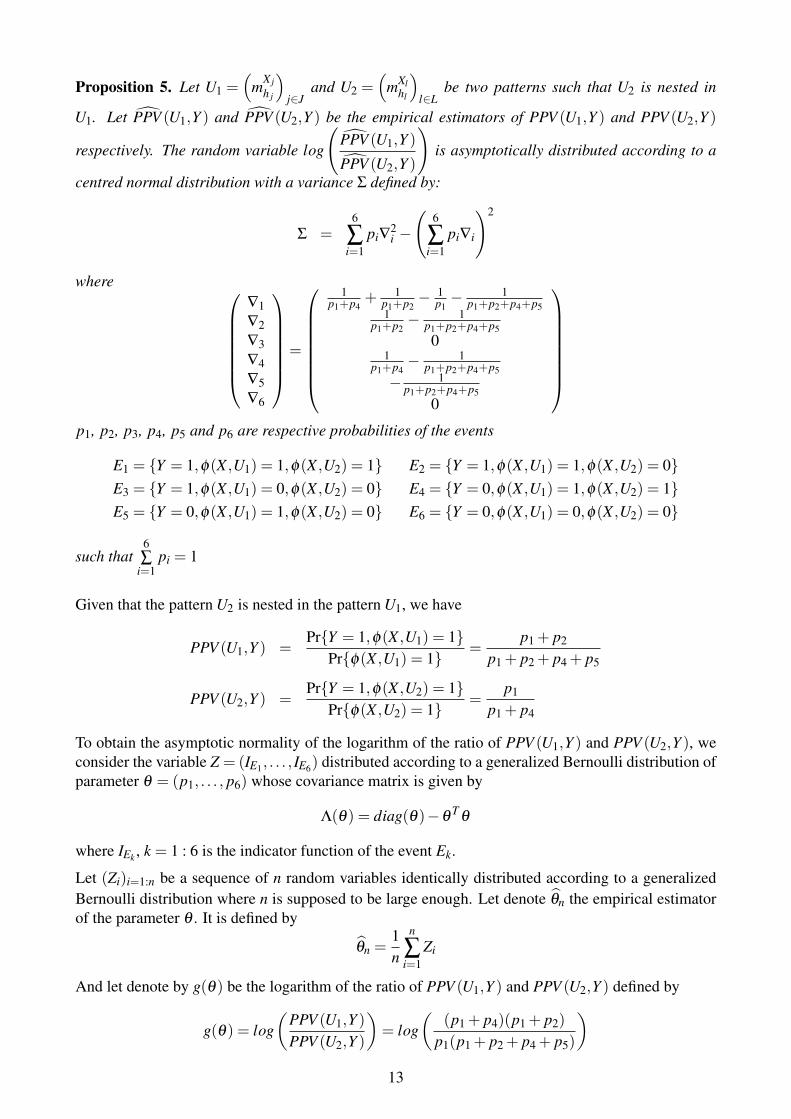
Proposition 5. Let U1 =(

mX jh j

)j∈J

and U2 =(

mXlhl

)l∈L

be two patterns such that U2 is nested in

U1. Let P̂PV (U1,Y ) and P̂PV (U2,Y ) be the empirical estimators of PPV (U1,Y ) and PPV (U2,Y )

respectively. The random variable log

(P̂PV (U1,Y )

P̂PV (U2,Y )

)is asymptotically distributed according to a

centred normal distribution with a variance Σ defined by:

Σ =6

∑i=1

pi∇2i −

(6

∑i=1

pi∇i

)2

where ∇1∇2∇3∇4∇5∇6

=

1p1+p4

+ 1p1+p2

− 1p1− 1

p1+p2+p4+p51

p1+p2− 1

p1+p2+p4+p50

1p1+p4

− 1p1+p2+p4+p5

− 1p1+p2+p4+p5

0

p1, p2, p3, p4, p5 and p6 are respective probabilities of the events

E1 = {Y = 1,φ(X ,U1) = 1,φ(X ,U2) = 1} E2 = {Y = 1,φ(X ,U1) = 1,φ(X ,U2) = 0}E3 = {Y = 1,φ(X ,U1) = 0,φ(X ,U2) = 0} E4 = {Y = 0,φ(X ,U1) = 1,φ(X ,U2) = 1}E5 = {Y = 0,φ(X ,U1) = 1,φ(X ,U2) = 0} E6 = {Y = 0,φ(X ,U1) = 0,φ(X ,U2) = 0}

such that6∑

i=1pi = 1

Given that the pattern U2 is nested in the pattern U1, we have

PPV (U1,Y ) =Pr{Y = 1,φ(X ,U1) = 1}

Pr{φ(X ,U1) = 1}=

p1 + p2

p1 + p2 + p4 + p5

PPV (U2,Y ) =Pr{Y = 1,φ(X ,U2) = 1}

Pr{φ(X ,U2) = 1}=

p1

p1 + p4

To obtain the asymptotic normality of the logarithm of the ratio of PPV (U1,Y ) and PPV (U2,Y ), weconsider the variable Z = (IE1, . . . , IE6) distributed according to a generalized Bernoulli distribution ofparameter θ = (p1, . . . , p6) whose covariance matrix is given by

Λ(θ) = diag(θ)−θT

θ

where IEk , k = 1 : 6 is the indicator function of the event Ek.

Let (Zi)i=1:n be a sequence of n random variables identically distributed according to a generalizedBernoulli distribution where n is supposed to be large enough. Let denote θ̂n the empirical estimatorof the parameter θ . It is defined by

θ̂n =1n

n

∑i=1

Zi

And let denote by g(θ) be the logarithm of the ratio of PPV (U1,Y ) and PPV (U2,Y ) defined by

g(θ) = log(

PPV (U1,Y )PPV (U2,Y )

)= log

((p1 + p4)(p1 + p2)

p1(p1 + p2 + p4 + p5)

)13

It result from the central limit theorem that√

n(

θ̂n−θ

)L−−→N (0,Λ(θ))

Using the multivariate delta method, we obtain that

√n(

g(θ̂n)−g(θ))

L−−→N(0,T

∇g(θ)Λ(θ)∇g(θ))

where

∇g(θ) =

∇1...

∇6

=

1p1+p4

+ 1p1+p2

− 1p1− 1

p1+p2+p4+p51

p1+p2− 1

p1+p2+p4+p50

1p1+p4

− 1p1+p2+p4+p5

− 1p1+p2+p4+p5

0

and

T∇g(θ)Λ(θ)∇g(θ) =

6

∑i=1

pi∇2i −

(6

∑i=1

pi∇i

)2

Using the continuity of the θ 7−→ ∇g(θ) and θ 7−→ Λ(θ) applications and the almost sure conver-gence of θ̂n to θ , we show that

T∇g(θ̂n)Λ(θ̂n)∇g(θ̂n)

p.s−−→ T∇g(θ)Λ(θ)∇g(θ)

It result from the Slutsky theorem that

√n(

g(θ̂n)−g(θ))

√T ∇g(θ̂n)Λ(θ̂n)∇g(θ̂n)

L−−→N (0,1)

Under the null hypothesis, we have g(θ) = 0. This allows us to build the following strategy to selectthe most relevant patterns.

1. Select the pattern U2 if

g(θ̂n)<−q1−α/2


n

2. Select the pattern U1 if

g(θ̂n)≥−q1−α/2


n

where q1−α/2 is the quantile of order 1−α/2 of the standard normal distribution.

14

Algorithm 2 Selecting procedure of the relevant patternsRequire: D a validation data set; Uλ a set of frequent and non redundant patternsEnsure: U ′

λa set of relevant patterns

for all C ∈Uλ doS← subset(C,Uλ )for all C′ ∈ S do

θ̂n← (p1, . . . , p6|D)

g(θ̂n)← log(V PP(C,Y |θ̂n))− log(V PP(C′,Y |θ̂n))

Λ(θ̂n)← diag(θ̂n)− θ̂ tnθ̂n

∇n← ∇g(θ̂n)end for

if there is C′ ∈ S such that g(θ̂n)<−q1−α/2

√∇t

nΛ(θ̂n)∇n

nthen

U ′λ← delete(C,Uλ )

elseU ′

λ← delete(S,Uλ )

end ifend for

The learning method, as described previously, requires a large database that will be subdivided intothree subsets of sufficiently large sizes (learning, validation and test). In the task of machine learning,it is common to encounter data whose size does not allow a subdivision of observations. Faced withsuch data, we can consider a bootstrap procedure.

5.2 Selecting a set of relevant patterns when sample is with small size

According to the central limit theorem, the following condition is true only when the number ofobservations is large enough.

Sn =

√n(

g(θ̂n)−g(θ))


L−−→N (0,1)

where n is the observations size.

In the case where the number of observations is small, it is not possible to have this condition forselecting a set of relevant patterns. This alternative method is to use a bootstrap hypothesis testing.The bootstrap is a well known re-sampling technique. The principle of the bootstrap method is toreplace the unknown distribution F that generated the sample by the distribution Fn which associatesto each observation a weight 1/n. So when drawing randomly with replacement n elements from ninitial observations, we obtain a bootstrap sample of size n by the empirical distribution Fn [7, 8].

Let g(θ) be our statistic of interest and Fg(θ) its sampling distribution. We can notice that Fg(θ)depend on the generalized Bernoulli distribution GZ of the random variable Z whose observed valuesare z1, . . . ,zn. Someone can write Fg(θ) = Fg(θ)(·,GZ), where GZ depend on the distribution FX of therandom variable X whose observed values are x1, . . . ,xn. In summary the sampling distribution FSdepend on the realisations z of the random variable Z and the distribution FX . We note

Fg(θ) = Fg(θ)(·,z,FX)

15

Since the FX distribution is unknown, we can replace it by the empirical distribution Fn of the observedvalues x1, . . . ,xn in the previous equality. Replace the unknown distribution FX by the empiricaldistribution Fn is equivalent to randomly draw with replacement n elements from the original datax1, . . . ,xn.Let g(θ̂n), a function of the sample X1, . . . ,Xn, denote an estimator of the unknown quantity g(θ), andwrite g(θ̂ ∗n ) the value of g(θ̂n) computed from a bootstrap sample X∗1 , . . . ,X

∗n drawn from the original

sample with replacement. We denote σ̂n =

√1n

(T ∇g(θ̂n)Λ(θ̂n)∇g(θ̂n)

)the standard deviation of

g(θ̂n). Let σ̂∗n denote the value of σ̂n computed for the bootstrap sample rather than the sample. Thenthe bootstrap distribution of

(g(θ̂ ∗n )−g(θ̂n)

)/σ̂∗n estimates the distribution of

(g(θ̂n)−g(θ)

)/σ̂n

under the null hypothesis [11]. To make hypotheses test with a null hypotheses H0 : g(θ) = 0 a gainsa n alternative hypotheses H1 : g(θ) 6= 0, we proceed as follow :

• First, we compute the value s0n of the statistic Sn for the sample X1, . . . ,Xn.

• Second, we simulate B resamples Xb1 , . . . ,X

bn (b = 1, . . . ,B) drawn from the sample with re-

placement. For each resample, we denote sbn the value of Sn computed the bth resample.

sbn =

g(θ̂ bn )−g(θ̂n)

σ̂bn

• third, we compute the bootstrap p− value

pn =1B

B

∑b=1

I(

Sbn > s0

n

)This allows us to build the following strategy to select the most relevant patterns.

(a) Select the pattern U2 if pn < α/2

(b) Select the pattern U2 if pn ≥ α/2

where α is the level of the test. We can notice that this hypothesis test allow to favour the shorterpatterns.

16

Algorithm 3 Selecting procedure of the relevant patternsRequire: D a validation data set ; Uλ a set of frequent and non redundant patterns ; α the level of

the test and B the number of bootstrap samples.Ensure: U ′

λa set of relevant patterns

for all C ∈Uλ doS← subset(C,Uλ )for all C′ ∈ S do

θ̂n← (p1, . . . , p6|D)

g(θ̂n)← log(V PP(C,Y |θ̂n))− log(V PP(C′,Y |θ̂n))

Λ(θ̂n)← diag(θ̂n)− θ̂ tnθ̂n

∇n← ∇g(θ̂n)

σ̂n←√

1n

(∇t

nΛ

(θ̂n

)∇n

)s0

n← g(θ̂n)/σ̂nfor all bootstrap sample Db do

θ̂ bn ← (p1, . . . , p6|Db)

g(θ̂ bn )← log(V PP(C,Y |θ̂ b

n ))− log(V PP(C′,Y |θ̂ bn ))

Λ(θ̂ bn )← diag(θ̂ b

n )− (θ̂ bn )

t θ̂n

∇n← ∇g(θ̂ bn )

σ̂bn ←

√1n

(∇t

nΛ

(θ̂ b

n

)∇n

)sb

n←(

g(θ̂ bn )−g(θ̂n)

)/σ̂b

n

end forpn← 1

B ∑Bb=1 I

(Sb

n > s0n)

if pn < α/2 then

U ′λ← delete(C,Uλ )

elseU ′

λ← delete(C′,Uλ )

end ifend for

end for

6 Empirical study

This section is about to evaluate our statistical learning method that we denote by PBBC (Pattern-Binary Based Classifier) on literature data and to compare its performances to standard classificationmethods. All the literature data that we have used for evaluating the PBBC are coming from UCImachine learning repository data sets [3]. All of them have two classes. The analysis of the proposedmethods were performed in the R environment for statistical computing [19]. The Association ruleswere explored by using the arules [1] package in the R environment for statistical computing. TheTable 3 is shows the dataset, the size in number of observations, the nominal and numerical attributesand the percentage of observations of the minority class.

17

DATASET SIZE ATTRIBUTES % TARGET CLASSNominal Numerical

Adult 45222 8 5 24.78Breast Cancer Wisconsin (Original) 699 10 0 34.50

Pima Indians Diabetes 768 0 8 34.89

Table 2: Datasets used for the evaluations

Since the data we have are not very unbalanced, we conducted several experiments by sup-sampling orsub-sampling the databases to obtain unbalanced samples for assessing the statistical learning method.We proceed as follows: we start by selecting the n observations of the prevailing class and we choosea proportion α of the rare class. Then we randomly select n′ = nα/(1−α) observations of therare class. Thus, we obtain a sample of n+ n′ observations which the proportion of the rare classobservations is equal to α .

For each simulated sample, we perform many combinations of the learning parameters c0,s0, l0 (i.e.we propose a dozen combinations of parameters values λ ). Thus each combination produces a clas-sifier for which we can compute its performances : sensitivity, specificity, error, etc. Then we selectthe classifier that realizes the best performances proceeding using a ROC curve.

The binary classification from logistic regression or binary regression trees involves fitting a paramet-ric or non-parametric model on the data D . This leads to the evaluation of conditional probabilitiesPr(Y = 1|X = x) depending on the data D . We obtain a classifier φ defined by

φ(x|α) =

{1 si Pr(Y = 1|X = x,D)> α

0 sinon

where α ∈]0,1[In the case of discriminant analysis or Bayesian networks analysis (eg naive Bayesian network), weconsider a prior law that we denote by π for the probability distribution of classes. Then a parametricor non parametric model based on the conditional probabilities Pr(X = x|Y = 1,D) is adjusted on thedata. The obtained classifier φ is defined as

φ(x|α) =

{1 si Pr(X = x|Y = 1,D)π(y)> α

0 sinon

where α ∈]0,1[This raises the issue of selecting an optimal classifier based on a compromise on performance mea-sures such as sensitivity, specificity, error rate, etc.. The ROC curve and the AUC measure are gener-ally used to achieve this goal.This approach can be extended to classifier aggregation methods such as binary tree boosting or ran-dom forest. Usually these methods use a threshold α = 0.5 by default. Very often the classifier φ(x|α)associated with threshold α = 0.5 does not provide better performance. And to compare our methodof classification with these methods, we consider the following strategy:

1. The first step is to determine the optimal learning parameters for adjusting an efficient model.

2. The second step is identify the optimal probability threshold. In other words, it is to iden-tify the threshold that produces the classifier whose performance measures provides the bestcompromise.

3. Then, we compare the performance of classifiers obtained with the performance of our classi-fier.

18

This approach has been compared to some competitor methods designed to deal with imbalancedclassification problem : SMOTE and ROSE.SMOTE is an over-sampling approach in which the minority class is over-sampled by creating "syn-thetic" examples rather than by over-sampling with replacement. The minority class is over-sampledby taking each minority class sample and introducing synthetic example along the line segments join-ing any/all the k minority class nearest neighbours. The application of SMOTE has been performedby choosing 5 nearest neighbours, as it was suggested by the authors in their paper [5].While ROSE is an an approach based on the generation of new artificial data from the classes, accord-ing to a smoothed bootstrap approach. It combines technique of over-sampling and under-samplingby generating an augmented sample of data thus helping the classifier in estimating a more accurateclassification rule [18]. The application of ROSE has been performed by fitting a logistic regressionmodel after to generate an augmented data by ROSE principle.

The results obtained are shown in Tables below. There were obtained using the caret (classificationand regression training ) package [14].

19

α = 0.007 α = 0.015Methods Sensibility Specificity Error AUC PSS Sensibility Specificity Error AUC PSS

PBBC 0.815 0.788 0.212 0.801 0.603 0.761 0.797 0.204 0.779 0.558ROSE 0.827 0.781 0.218 0.804 0.608 0.835 0.777 0.222 0.806 0.612SMOTE 0.716 0.729 0.271 0.723 0.445 0.801 0.675 0.323 0.738 0.476Random.F 0.259 0.996 0.009 0.628 0.255 0.330 0.987 0.023 0.658 0.317Boosting 0.210 0.999 0.007 0.604 0.208 0.278 0.996 0.015 0.637 0.275CART 0.173 0.999 0.007 0.586 0.172 0.210 0.999 0.012 0.605 0.210CTREE 0.185 0.999 0.007 0.592 0.184 0.205 0.999 0.013 0.602 0.203Boost.glm 0.023 0.928 0.008 0.525 -0.049 0.026 0.928 0.016 0.523 -0.045N.Bayes 0.160 0.999 0.007 0.580 0.160 0.131 0.999 0.014 0.565 0.130


PBBC 0.773 0.798 0.203 0.786 0.571 0.739 0.832 0.175 0.785 0.570ROSE 0.838 0.787 0.211 0.812 0.625 0.811 0.777 0.220 0.794 0.589SMOTE 0.770 0.727 0.271 0.749 0.498 0.791 0.778 0.221 0.784 0.569Random.F 0.406 0.975 0.042 0.691 0.381 0.604 0.919 0.103 0.762 0.523Boosting 0.378 0.990 0.028 0.684 0.368 0.608 0.947 0.076 0.778 0.555CART 0.241 0.999 0.024 0.620 0.240 0.488 0.948 0.084 0.718 0.436CTREE 0.249 0.997 0.026 0.623 0.246 0.568 0.940 0.086 0.754 0.508Boost.glm 0.135 0.926 0.030 0.530 0.061 0.465 0.887 0.080 0.676 0.352N.Bayes 0.143 0.997 0.028 0.570 0.140 0.196 0.996 0.060 0.596 0.191



Table 3: Sensibility, specificity, error estimation, area under the ROC curve and Pierce score, with different baseclassification rules, with different proportions (α) of the target class, for Adult dataset. This performances are performedon test sample which distribution is identical to distribution of training sample

20


PBBC 0.826 0.678 0.286 0.752 0.503 0.839 0.720 0.251 0.780 0.558ROSE 0.807 0.749 0.237 0.778 0.556 0.832 0.762 0.221 0.797 0.594SMOTE 0.173 0.986 0.214 0.580 0.159 0.220 0.988 0.201 0.604 0.208Random.F 0.248 0.995 0.189 0.622 0.243 0.320 0.987 0.177 0.653 0.307Boosting 0.232 0.999 0.190 0.615 0.231 0.270 0.996 0.183 0.633 0.267CART 0.169 0.999 0.205 0.584 0.168 0.150 0.999 0.210 0.575 0.150CTREE 0.169 0.999 0.205 0.584 0.168 0.199 0.998 0.199 0.598 0.197Boost.glm 0.021 0.928 0.241 0.526 -0.051 0.022 0.928 0.241 0.525 -0.050N.Bayes 0.123 0.999 0.217 0.561 0.122 0.142 0.999 0.212 0.570 0.140





Table 4: Sensibility, specificity, error estimation, area under the ROC curve and Pierce score, with different baseclassification rules, with different proportions (α) of the target class, for Adult Data Set. This performances are performedon test sample which distribution is different to distribution of training sample

21


PBBC 0.999 0.939 0.059 0.970 0.939 0.971 0.884 0.110 0.928 0.855ROSE 0.881 0.930 0.072 0.905 0.810 0.979 0.952 0.046 0.965 0.931SMOTE 0.798 0.984 0.022 0.891 0.782 0.926 0.988 0.016 0.957 0.914Boosting 0.786 0.960 0.045 0.873 0.746 0.973 0.934 0.063 0.954 0.907Random.F 0.964 0.925 0.074 0.945 0.889 0.985 0.943 0.054 0.964 0.928Boost.glm 0.750 0.969 0.038 0.860 0.719 0.994 0.944 0.053 0.969 0.938CATR 0.470 0.984 0.032 0.727 0.454 0.847 0.979 0.030 0.913 0.826CTREE 0.786 0.947 0.058 0.866 0.732 0.947 0.950 0.050 0.949 0.897N.Bayes 0.893 0.970 0.032 0.931 0.863 0.952 0.970 0.031 0.961 0.921


PBBC 0.981 0.861 0.120 0.921 0.843 0.995 0.887 0.081 0.941 0.882ROSE 0.976 0.958 0.039 0.967 0.935 0.989 0.963 0.029 0.976 0.952SMOTE 0.957 0.978 0.026 0.967 0.934 0.976 0.974 0.026 0.975 0.950Boosting 0.941 0.961 0.042 0.951 0.901 0.972 0.951 0.043 0.962 0.923Random.F 0.987 0.950 0.044 0.969 0.937 0.978 0.967 0.030 0.972 0.945Boost.glm 0.991 0.932 0.059 0.962 0.924 0.962 0.959 0.040 0.961 0.921CART 0.905 0.969 0.041 0.937 0.874 0.936 0.955 0.051 0.946 0.891CTREE 0.949 0.925 0.071 0.937 0.874 0.976 0.934 0.054 0.955 0.909N.Bayes 0.964 0.971 0.030 0.967 0.935 0.988 0.965 0.028 0.976 0.953

Table 5: Sensibility, specificity, error estimation, area under the ROC curve and Pierse score, with different baseclassification rules, with different proportions (α) of the target class, for Breast Cancer Data Set.

22


PBBC 0.572 0.854 0.154 0.713 0.426 0.550 0.729 0.284 0.639 0.279ROSE 0.975 0.573 0.415 0.774 0.548 0.693 0.806 0.201 0.749 0.499SMOTE 0.533 0.971 0.042 0.752 0.504 0.620 0.946 0.075 0.783 0.567Boosting 0.800 0.833 0.168 0.817 0.633 0.648 0.773 0.235 0.711 0.421Random.F 0.544 0.703 0.302 0.623 0.246 0.482 0.880 0.146 0.681 0.363Boost.glm 0.031 0.894 0.132 0.537 -0.075 0.310 0.846 0.189 0.578 0.156CART 0.329 0.504 0.501 0.583 -0.167 0.323 0.911 0.128 0.617 0.234CTREE 0.544 0.861 0.149 0.702 0.405 0.501 0.778 0.240 0.639 0.279N.Bayes 0.469 0.854 0.157 0.661 0.323 0.658 0.783 0.226 0.720 0.441


PBBC 0.723 0.673 0.320 0.698 0.396 0.718 0.733 0.271 0.726 0.451ROSE 0.695 0.790 0.224 0.742 0.485 0.819 0.705 0.263 0.762 0.524SMOTE 0.796 0.858 0.151 0.827 0.654 0.808 0.855 0.158 0.831 0.663Boosting 0.760 0.754 0.245 0.757 0.514 0.736 0.783 0.230 0.760 0.520Random.F 0.866 0.708 0.270 0.787 0.573 0.802 0.741 0.242 0.772 0.543Boost.glm 0.509 0.756 0.279 0.633 0.266 0.617 0.778 0.268 0.698 0.395CART 0.535 0.843 0.202 0.689 0.378 0.723 0.716 0.282 0.719 0.439CTREE 0.693 0.674 0.323 0.684 0.368 0.717 0.738 0.268 0.727 0.454N.Bayes 0.784 0.751 0.244 0.768 0.535 0.806 0.710 0.263 0.758 0.516

Table 6: Sensibility, specificity, error estimation, area under the ROC curve and Pierce score, with different baseclassification rules, with different proportions (α) of the target class, for Pima Indians Diabetes Data Set.

7 discussion

Association rules learning is a well known method in the area of data-mining. It is a research approachfor discovering interesting relationships between feature variables in large database. Some algorithmssuch that linear and logistic regression, k-nearest-neighbour, and Kmeans clusters are "main effect"models and are not able to manage missing values and/or to identify interactions automatically. How-ever the ability to take in account interaction and to manage missing values in building effectivepredictive models for accurate classification is sometime critical. The main advantages of dealingwith association rules learning for classification are : first we don’t need to delete missing values toperform it and second it can be used to find the best interactions by searching exhaustively all possiblecombinations of interactions and listing them through association rules.

It appears from the results of Tables 3, 4 that when we are dealing with unbalanced and large datasetthe PBBC method is better to use than the Naive Bayes algorithm, the CTREE algorithm, the CARTalgorithm, Boosting tree algorithm, Boosting generalize linear model algorithm and Random Forestalgorithm. The PBBC method produces approximately the same estimation performance than ROSEalgorithm and SMOTE algorithm. Moreover when response variable distribution in training sample isdifferent to response variable distribution in test sample the PBBC method is significantly better thanSMOTE algorithm when target class occurrence is less than 15%.When we are dealing with unbalanced and small dataset the results from Tables 5 and 6 show thanthe PBBC method produces approximately the same estimations than alternatives methods. The main

23

advantage of the PBBC method to others methods such that random forest and boosting methods isthat one can present the classifier built by PBBC as an structure tree( see Figure 3).

In the following table, we sample twenty four classifiers built from unbalanced Adult dataset wherethe occurrence of the target class is equal to α = 0.7%. We set the minimum support threshold(Min.sup) from {3.510−4,4.210−4,4.910−4,5.610−4,6.310−4,7.010−4} and the minimum confi-dence threshold (Min.conf) from {0.02,0.03,0.04,0.05}. The process of the PBBC method yieldstwenty four classifiers for which the estimations of their performances are presented in the Table 7.

Min.sup Min.conf Sensibility Specificity Error AUC PSS1 3.5 10−4 0.02 0.85 0.68 0.32 0.77 0.532 3.5 10−4 0.03 0.86 0.70 0.30 0.78 0.573 3.5 10−4 0.04 0.77 0.79 0.21 0.78 0.554 3.5 10−4 0.05 0.72 0.84 0.16 0.78 0.565 4.2 10−4 0.02 0.88 0.68 0.32 0.78 0.556 4.2 10−4 0.03 0.86 0.70 0.30 0.78 0.577 4.2 10−4 0.04 0.77 0.79 0.21 0.78 0.558 4.2 10−4 0.05 0.72 0.84 0.16 0.78 0.569 4.9 10−4 0.02 0.77 0.76 0.24 0.76 0.52

10 4.9 10−4 0.03 0.85 0.74 0.26 0.80 0.5911 4.9 10−4 0.04 0.74 0.82 0.18 0.78 0.5612 4.9 10−4 0.05 0.69 0.86 0.14 0.78 0.5513 5.6 10−4 0.02 0.77 0.73 0.27 0.75 0.4914 5.6 10−4 0.03 0.85 0.73 0.27 0.79 0.5815 5.6 10−4 0.04 0.80 0.79 0.21 0.80 0.5916 5.6 10−4 0.05 0.62 0.88 0.12 0.75 0.4917 6.3 10−4 0.02 0.68 0.78 0.22 0.73 0.4618 6.3 10−4 0.03 0.85 0.74 0.26 0.79 0.5919 6.3 10−4 0.04 0.79 0.79 0.21 0.79 0.5820 6.3 10−4 0.05 0.62 0.88 0.12 0.75 0.5021 7.0 10−4 0.02 0.77 0.74 0.26 0.75 0.5022 7.0 10−4 0.03 0.84 0.74 0.26 0.79 0.5823 7.0 10−4 0.04 0.77 0.80 0.20 0.78 0.5624 7.0 10−4 0.05 0.59 0.89 0.11 0.74 0.48

Table 7: Performance estimation of twenty four classifiers using α = 0.7% as proportion of the rareclass both in the training set and in the test dataset.

**

**

**

****

****

*

**

*

*

*

**

*

*

0.0 0.2 0.4 0.6 0.8 1.0

0.0

0.2

0.4

0.6

0.8

1.0

1 − Specificity

Sen

sibi

lity

Figure 1:

24

The optimal classifier (best sensibility, best specificity and best area under the ROC curve) is givenby following learning parameter : Min.sup = 4.910−4 and Min.conf = 0.03. These above learningparameters were used to produce an initial set of 271 patterns. The pruning procedure of redundantpatterns has allowed to eliminate 121 profiles. The re-evaluation of the performances of the 150remaining patterns using the validation sample has allowed to identify five patterns whose supportsare zero. And the step of selecting relevant patterns has allowed to extract 24 relevant patterns amongthe 145 non redundant patterns remaining. The optimal classifier is presented follow as an structuretree (in two parts) that can help to visualise most relevant patterns selected from the sample.

TotalPopulation

minority.group=White

gender= Male

educ= Assoc-vocPPV=0.4%; TPR=1%

occup= Exec-managerialPPV=2%; TPR=17%

educ= Bachelors

age=46-54PPV=4%; TPR=9%

age=38-46PPV=2%; TPR=7%

marital.status=Married-civ-spouse

occup= SalesPPV=2%; TPR=9%

workclass= Self-emp-incPPV=2%; TPR=4%

workclass= Self-emp-inc

gender= MalePPV=1%; TPR=4%

cgain=10000-InfPPV=58%; TPR=9%

cgain=5000-10000PPV=8%; TPR=7%

closs=1750-1950PPV=11%; TPR=5%

educ= MastersPPV=2%; TPR=11%

Figure 2: Presentation of the first part of the structure tree of the optimal classifier among the twentyfour classifiers

25

TotalPopulation

hourpw = 50-65

gender= Male

age=38-46PPV=4%; TPR=11%

educ= BachelorsPPV=5%; TPR=11%



age=38-46PPV=3%; TPR=10%

occup= Prof-specialtyPPV=3%; TPR=9%


workclass= Pri-vate

marital.status=Married-civ-spouse

age=46-54PPV=2%; TPR=9%

occup= Exec-managerial

gender= MalePPV=2%; TPR=10%

hourpw=42-50 age=38-46PPV=2%; TPR=4%

relation= Husband


occup= SalesPPV=1%; TPR=6%

occup= Prof-specialtyPPV=4%; TPR=15%



Figure 3: Presentation of the second part of the structure tree of the optimal classifier among thetwenty four classifiers

26

8 Conclusion

This paper aims at advocating a methodology to state a binary classification function when dealingwith a classification task where the target class is a rare event. Assuming that a large amount of datais available, this goal is achieved by resorting to association rules for exploring the data in order toidentify the patterns that are correlated with the target class. Relevant patterns are selected on thebasis of their relative risk, their true-positive rates and true-negative rates. The procedure allows toovercome the short-coming of the regression methods which underestimate the conditional probabil-ities of the occurrence of the target class when the frequency of the instances which belong to thisclass is very low. Moreover patterns of attributes’ interactions which are highly correlated with targetclass are specified, thus the classification function does not appear like a black-box. Nevertheless oneshould notice that a stage of data preprocessing is needed before performing the procedure since it isassumed that the covariates are evaluated on a non-numerical scale. The effectiveness of the proposedmethod is shown by its application to a real world data related to the study of in-hospital maternalmortality.

27

References

[1] AGRAWAL, R., AND SRIKANT, R. Fast algorithms for mining association rules in largedatabases. In Proceedings of the 20th International Conference on Very Large Data Bases (SanFrancisco, CA, USA, 1994), VLDB ’94, Morgan Kaufmann Publishers Inc., pp. 487–499.

[2] AN, A., AND CERCONE, N. Discretization of continuous attributes for learning classifi-cation rules. In Methodologies for Knowledge Discovery and Data Mining, N. Zhong andL. Zhou, Eds., no. 1574 in Lecture Notes in Computer Science. Springer Berlin Heidelberg,1999, pp. 509–514.

[3] BACHE, K., AND LICHMAN, M. UCI machine learning repository[http://archive.ics.uci.edu/ml]. Tech. rep., University of California, Irvine, School of In-formation and Computer Sciences, 2013.

[4] BREIMAN L. Bagging predictors. Kluwer Academic Publishers, Boston. Manufactured in TheNetherlands Machine Learning, 24 (1996), 123–140.

[5] CHAWLA, N. V., BOWYER, K. W., HALL, L. O., AND KEGELMEYER, W. P. Smote: Syntheticminority over-sampling technique. Journal of Artificial Intelligence Research 16 (2002), 321–357.

[6] CLARKE, E. J., AND BARTON, B. A. Entropy and MDL discretization of continuous variablesfor bayesian belief networks. International Journal of Intelligent Systems 15, 1 (2000), 61–92.

[7] EFRON, B. The jackknife, the bootstrap, and other resampling plans. Society for Industrial andApplied Mathematics, Philadelphia, Pa., 1982.

[8] EFRON, B., AND TIBSHIRANI, R. J. An Introduction to the Bootstrap. Taylor & Francis, 1994.

[9] FAYYAD, U. M., AND IRANI, K. B. On the handling of continuous-valued attributes in decisiontree generation. Machine Learning 8 (1992), 87–102.

[10] FAYYAD, U. M., AND IRANI, K. B. Multi-interval discretization of continuous-valued at-tributes for classification learning. Artificial Intelligence 13 (1993), 1022–1027.

[11] HALL, P., AND WILSON, S. R. Two guidelines for bootstrap hypothesis testing. Biometrics47, 2 (1991), 757–762.

[12] HUALIN WANG, XIAOGANG SU. Bagging probit models for unbalanced classification. IGIGlobal ch017 (2010), 290–296.

[13] KOHAVI, R. Scaling up the accuracy of naive-bayes classifiers: a decision-tree hybrid. InProceedings of the Second International Conference on Knowledge Discovery and Data Mining(1996), p. to appear.

[14] KUHN, M. Building predictive models in r using the caret package. Journal of StatisticalSoftware 28, 05 (2008).

[15] LI J, ADA W F AND FAHEY P. Efficient discovery of risk patterns in medical data. ArtificialIntelligence in Medecine 45 (2009), 77–89.

[16] LI J, ADA W F, HONGXING HE, JIE CHEN, HUIDONG JIN, MCAULLAY D, GRAHAM W,SPARKS R AND KELMAN C. Mining risk in medical data. KDD 05, ILLinois, USA (August21-24, 2005).

28

[17] LIU, B., HSU, W., AND MA, Y. Integrating classification and association rule mining. pp. 80–86.

[18] MENARDI, G., AND TORELLI, N. Training and assessing classification rules with imbalanceddata. Data Mining and Knowledge Discovery (2014), 92–122.

[19] R CORE TEAM. R: A Language and Environment for Statistical Computing. R Foundation forStatistical Computing, Vienna, Austria, 2013.

[20] SCARPA B AND TORELLI N. Selection the training set in classification problem with rare event.

29

Documents

Cheikh Ndour Simplice Dossou Gbété Abstract arXiv:1202