Performance analysis of multi-server queueing system operating under control of a random environment 317

Performance analysis of multi-server queueing system operating under control of a random environment

Che Soong Kim, Alexander Dudin, Valentina Klimenok and Valentina Khramova

X

Performance analysis of multi-server queueing system operating under control of a random environment

Che Soong Kim1, Alexander Dudin2, Valentina Klimenok2,

and Valentina Khramova2 1Sangji University

Korea 2Belarusian State University

Belarus

1. Introduction

Since the early 1900th the Erlang multi-server queueing systems with losses ( B -model or 0M/M/N/ system) and with an infinite size buffer ( C -model or M/M/N system) provided

good mathematical tools for capacity planning and performance evaluation in the classic telephone networks for many years. Good quality of the loss probability forecasting in real world networks based on the formulas obtained for the 0M/M/N/ system and the delay prediction based on the formula obtained for the M/M/N system was a rather surprising because the requirement that inter-arrival and service times have an exponential distribution, which is imposed in the 0M/M/N/ and M/M/N models, seems to be too strict. The interest of mathematicians to the fact of good matching of the calculated under debatable assumptions characteristics to their measured value in real world systems have lead to the following two results. By efforts of many mathematicians (A. Ya. Khinchin and B. I. Grigelionis first of all), it was proved that the superposition of a large number of independent flows having uniformly small intensity approaches to the stationary Poisson input when the number of the superposed inputs tends to infinity. It explains the fact that the flows in classic telephone networks (where flows are composed by small individual flows from independent subscribers) have the exponentially distributed inter-arrival times. Concerning the service time distribution, situation was more complicated. The real-life measurements have shown that the service (conversation) time can not be well approximated by means of the exponentially distributed random variable. So, due to the good matching of results obtained for the 0M/M/N/ queue performance characteristics to characteristics of real systems modelled by such a queue, the hypothesis has arisen that the stationary state distribution in the 0M/M/N/ queue is the same as the one in the 0M/G/N/

15

www.intechopen.com

Trends in Telecommunications Technologies318

queue conditional that the average service times in both models coincide. This property was called the invariant (or insensitivity) property of the model with respect to the service time distribution. The work [10] by B. A. Sevastjanov is the first one where this property was proven strictly. So, the question why the Erlang's models give very good results for a practice was highlighted. The special books containing the tables for a loss probability under the given values of the number N of channels and intensities of the input and service exist. Different design problems (for a fixed value of permissible loss probability, to find the maximal intensity of the flow, which can be served by the line consisting of a fixed number of channels under the fixed average service time, or to find the necessary number of channels sufficient for transmission of the flow with a fixed intensity, etc) are solved by means of these tables. However, the flows in the modern telecommunication networks have lost the nice properties of their predecessors in the old classic networks. In opposite to the stationary Poisson input (stationary ordinary input with no aftereffect), the modern real life flows are non-stationary, group and correlated. The BMAP (Batch Markovian Arrival Process) arrival process was introduced as a versatile Markovian point process (VMPP ) by M.F. Neuts in the 70th. The original development of VMPP contained extensive notations; however these notations were simplified greatly in [7] and ever since this process bears the name BMAP . The class of BMAP s includes many input flows considered previously, such as stationary Poisson ( M ), Erlangian ( kE ), Hyper-Markovian ( HM ), Phase-Type ( PH ), Interrupted Poisson Process ( IPP ), Markov Modulated Poisson Process ( MMPP ). Generally speaking, the BMAP is correlated, so it is ideal to model correlated and (or) bursty traffic in modern telecommunication networks. As it was mentioned above, the question why the inter-arrival times in the classical networks have the exponential distribution was answered in literature. However, Erlang's assumption that the service time distribution has the exponential distribution is not supported by the real networks measurements. In the case of the 0M/M/N/ system, good fitting of performance measures of this system with the respective measures of real world systems is easy explained by Sevastjanov's result. But in the case of the M/M/N system, it was necessary to generalize results by Erlang to the cases of another, than exponential, service time distributions. This work was started by Erlang who offered so called Erlang's distribution. He introduced Erlangian of order k distribution as a distribution of a sum of k independent identically exponentially distributed random variables (phases). Further, so called phase type ( PH ) distribution was introduced into consideration as the straightforward generalization of Erlangian distribution, see, e.g., [8]. PH distribution includes as the special cases the exponential, Erlangian, Hyper-exponential, Coxian distributions. In our chapter we assume that service times at the fixed operation mode of the system have PH distribution. It follows from discussion above that it is interesting to extend investigation of Erlang's models to the case of the BMAP input and PH type service process. This work was started by M. Combe in [1] and V. Klimenok in [5] where the BMAP/M/N and 0BMAP/M/N/ models, respectively, were investigated. In paper [2], we investigated the 0BMAP/PH/N/ model having no buffer. It was shown there that the stationary distribution of the system states essentially depends on the shape of

the service time distribution and so Sevastjanov's invariant property does not hold true in the case of the general BMAP arrival process. Here we analyze the BMAP/PH/N/L system with a finite buffer and the BMAP/PH/N system with infinite buffer. Simultaneously, we make one more essential generalization of the model under study. Motivation of this generalization is as follows. Even if one will use such general models of the arrival and service process as the BMAP and PH , he may fail in application to practical systems. The reason is the following. Assumption that the input flow is described by the BMAP allows to take into consideration a burstiness, an effect of correlation in the arrival process and variation of inter-arrival times. Assumption that the service process is described by the PH distribution allows to take into consideration variation of service times. But the BMAP arrival process and PH service process are assumed to be stationary and independent of each other within the borders of the models of BMAP/PH/N/L type, 0 . L While in many real world systems the input and service processes are not absolutely stable and may be mutually dependent. They may be influenced by some external factors, e.g., the different level of the noise in the transmission channel, hardware degradation and recovering, change of the distance by a mobile user from the base station, parallel transmission of high priority information, etc. Information transmission channel modeled by means of the BMAP/PH/N/L queueing system can be a part of complex communication network. The rest of the network may essentially vary characteristics of the arrival and service process in this system by means of: (i) changing the bandwidth of the channel (due to reliability factors or the needs to provide good quality of service in another parts of the network when congestion occurs); (ii) changing the mean arrival rate due breakdowns, overflow or underflow of alternative information transmission channels. Thus, to get the mathematical tool for adequate modeling such information transmission channels, more complicated queues than the BMAP/PH/N/L queueing system should be analyzed. These queues, in addition to the account of complicated internal structure of the arrival and service processes by means of considering the BMAP and ,PH must take into account the influence of random external factors. In some extent, it can be done by means of analyzing the models of queues operating in a random environment. Such an analysis is the topic of this chapter. Importance of investigation of the queues operating in a random environment ( RE ) drastically increased in the last years due to the following reason. The flows of information in the modern communication networks are essentially heterogeneous. Some types of information are very sensitive with respect to a delay and an jitter but tolerant with respect to losses. Another ones are tolerant with respect to the delay but very sensitive with respect to the loss of the packets. So, different schemes of the dynamic bandwidth sharing among these types exist and are developing. They assume that, in the case of congestion, transmission of the delay tolerant flows is temporarily postponed to provide better conditions for transmission of the delay sensitive flows. Analysis of such schemes requires the probabilistic analysis of the multi-dimensional processes describing transmission process of the different flows. This analysis is often impossible due to the mathematical complexity. In such a case, it is reasonable to decompose a simultaneous consideration of all flows to separate analysis of the processes of transmission of the delay sensitive and the delay tolerant flows. To this end, we model transmission of the delay sensitive flows in terms of the queues with the controlled service or (and) arrival rate where the service or the

www.intechopen.com

Performance analysis of multi-server queueing system operating under control of a random environment 319

queue conditional that the average service times in both models coincide. This property was called the invariant (or insensitivity) property of the model with respect to the service time distribution. The work [10] by B. A. Sevastjanov is the first one where this property was proven strictly. So, the question why the Erlang's models give very good results for a practice was highlighted. The special books containing the tables for a loss probability under the given values of the number N of channels and intensities of the input and service exist. Different design problems (for a fixed value of permissible loss probability, to find the maximal intensity of the flow, which can be served by the line consisting of a fixed number of channels under the fixed average service time, or to find the necessary number of channels sufficient for transmission of the flow with a fixed intensity, etc) are solved by means of these tables. However, the flows in the modern telecommunication networks have lost the nice properties of their predecessors in the old classic networks. In opposite to the stationary Poisson input (stationary ordinary input with no aftereffect), the modern real life flows are non-stationary, group and correlated. The BMAP (Batch Markovian Arrival Process) arrival process was introduced as a versatile Markovian point process (VMPP ) by M.F. Neuts in the 70th. The original development of VMPP contained extensive notations; however these notations were simplified greatly in [7] and ever since this process bears the name BMAP . The class of BMAP s includes many input flows considered previously, such as stationary Poisson ( M ), Erlangian ( kE ), Hyper-Markovian ( HM ), Phase-Type ( PH ), Interrupted Poisson Process ( IPP ), Markov Modulated Poisson Process ( MMPP ). Generally speaking, the BMAP is correlated, so it is ideal to model correlated and (or) bursty traffic in modern telecommunication networks. As it was mentioned above, the question why the inter-arrival times in the classical networks have the exponential distribution was answered in literature. However, Erlang's assumption that the service time distribution has the exponential distribution is not supported by the real networks measurements. In the case of the 0M/M/N/ system, good fitting of performance measures of this system with the respective measures of real world systems is easy explained by Sevastjanov's result. But in the case of the M/M/N system, it was necessary to generalize results by Erlang to the cases of another, than exponential, service time distributions. This work was started by Erlang who offered so called Erlang's distribution. He introduced Erlangian of order k distribution as a distribution of a sum of k independent identically exponentially distributed random variables (phases). Further, so called phase type ( PH ) distribution was introduced into consideration as the straightforward generalization of Erlangian distribution, see, e.g., [8]. PH distribution includes as the special cases the exponential, Erlangian, Hyper-exponential, Coxian distributions. In our chapter we assume that service times at the fixed operation mode of the system have PH distribution. It follows from discussion above that it is interesting to extend investigation of Erlang's models to the case of the BMAP input and PH type service process. This work was started by M. Combe in [1] and V. Klimenok in [5] where the BMAP/M/N and 0BMAP/M/N/ models, respectively, were investigated. In paper [2], we investigated the 0BMAP/PH/N/ model having no buffer. It was shown there that the stationary distribution of the system states essentially depends on the shape of

the service time distribution and so Sevastjanov's invariant property does not hold true in the case of the general BMAP arrival process. Here we analyze the BMAP/PH/N/L system with a finite buffer and the BMAP/PH/N system with infinite buffer. Simultaneously, we make one more essential generalization of the model under study. Motivation of this generalization is as follows. Even if one will use such general models of the arrival and service process as the BMAP and PH , he may fail in application to practical systems. The reason is the following. Assumption that the input flow is described by the BMAP allows to take into consideration a burstiness, an effect of correlation in the arrival process and variation of inter-arrival times. Assumption that the service process is described by the PH distribution allows to take into consideration variation of service times. But the BMAP arrival process and PH service process are assumed to be stationary and independent of each other within the borders of the models of BMAP/PH/N/L type, 0 . L While in many real world systems the input and service processes are not absolutely stable and may be mutually dependent. They may be influenced by some external factors, e.g., the different level of the noise in the transmission channel, hardware degradation and recovering, change of the distance by a mobile user from the base station, parallel transmission of high priority information, etc. Information transmission channel modeled by means of the BMAP/PH/N/L queueing system can be a part of complex communication network. The rest of the network may essentially vary characteristics of the arrival and service process in this system by means of: (i) changing the bandwidth of the channel (due to reliability factors or the needs to provide good quality of service in another parts of the network when congestion occurs); (ii) changing the mean arrival rate due breakdowns, overflow or underflow of alternative information transmission channels. Thus, to get the mathematical tool for adequate modeling such information transmission channels, more complicated queues than the BMAP/PH/N/L queueing system should be analyzed. These queues, in addition to the account of complicated internal structure of the arrival and service processes by means of considering the BMAP and ,PH must take into account the influence of random external factors. In some extent, it can be done by means of analyzing the models of queues operating in a random environment. Such an analysis is the topic of this chapter. Importance of investigation of the queues operating in a random environment ( RE ) drastically increased in the last years due to the following reason. The flows of information in the modern communication networks are essentially heterogeneous. Some types of information are very sensitive with respect to a delay and an jitter but tolerant with respect to losses. Another ones are tolerant with respect to the delay but very sensitive with respect to the loss of the packets. So, different schemes of the dynamic bandwidth sharing among these types exist and are developing. They assume that, in the case of congestion, transmission of the delay tolerant flows is temporarily postponed to provide better conditions for transmission of the delay sensitive flows. Analysis of such schemes requires the probabilistic analysis of the multi-dimensional processes describing transmission process of the different flows. This analysis is often impossible due to the mathematical complexity. In such a case, it is reasonable to decompose a simultaneous consideration of all flows to separate analysis of the processes of transmission of the delay sensitive and the delay tolerant flows. To this end, we model transmission of the delay sensitive flows in terms of the queues with the controlled service or (and) arrival rate where the service or the

www.intechopen.com

Trends in Telecommunications Technologies320

arrival rate can be changed depending on the queue length or the waiting time. Redistribution of a bandwidth to avoid congestion for the delay sensitive flows causes a variation, at random moments, of an available bandwidth for the delay tolerant flows. Correspondingly, the queues operating in a random environment naturally arise as the mathematical model for the delay tolerant flows transmission. Mention that the 0BMAP/PH/N/ model operating in the RE was recently investigated in [4]. Short overview of the recent research of queues operating in the RE can be found there. In this chapter, we consider the models BMAP/PH/N/L and BMAP/PH/N operating in the

.RE

2. The Mathematical Model

We consider the queueing system having N identical servers. The system behavior depends on the state of the stochastic process (random environment) 0,tr t which is assumed to be an irreducible continuous time Markov chain with the state space {1, , }R ,

2R , and the infinitesimal generator Q. The input flow into the system is the following modification of the BMAP . In this input flow, the arrival of batches is directed by the process 0,t t (the underlying process) with the state space {0 1 }, ,… , W . Under the fixed state r of the ,RE this process behaves as an irreducible continuous time Markov chain. Intensities of transitions of the chain 0,t t which are accompanied by arrival of k -size batch, are described by the matrices ( ) 0r

kD k ,

1, ,r R with the generating function

( ) ( )

0( ) 1.r r k

kk

D z D z z The matrix ( )(1)rD is an

irreducible generator for all 1, .r R Under the fixed state r of the random environment, the average intensity ( )r (fundamental rate) of the BMAP is defined as

( ) ( ) ( )1( )r r r

zD z ,e and the intensity ( )rb of batch arrivals is defined as

( ) ( ) ( )0 .r r r

b D e Here the row vector ( )r is the solution to the equations

( ) ( ) ( )(1) , 1,r r rD 0 e e is a column vector of appropriate size consisting of 1's. The variation coefficient ( )r

varc of intervals between batch arrivals is given by 2 ( ) ( ) ( ) 1

02 ( ) 1,r r r(r)var bc D e

while the correlation coefficient ( )r

corc of intervals between successive batch arrivals is calculated as 2( ) ( ) ( ) ( ) ( ) ( ) ( ) ( )1 1

0 0 0( ) ( (1) )( ) 1r r r r r r r rcor b varc D D D D ce -

At the epochs of the process 0,tr t transitions, the state of the process 0,t t is not changed, but the intensities of its transitions are immediately changed.

The service process is defined by the modification of the PH -type service time distribution. Service time is interpreted as the time until the irreducible continuous time Markov chain

0,tm t with the state space {0 1 1}, ,… , M reaches the absorbing state 1.M Under the fixed value r of the random environment, transitions of the chain 0,tm t within the state space {1 },… , M are defined by an irreducible sub-generator ( )rS while the intensities of transition into the absorbing state are defined by the vector ( ) ( )

0 .r rSS e At the service beginning epoch, the state of the process 0,tm t is chosen according to the probabilistic

row vector ( ) , 1, .r r R It is assumed that the state of the process 0,tm t is not changed at the epoch of the process 0,tr t transitions. Just the exponentially distributed sojourn time of the process 0,tm t in the current state is re-started with a new intensity defined by the sub-generator corresponding to the new state of the random environment 0.tr t The system under consideration has 0L, , L waiting positions. In the case of an infinite buffer ( L = ) all customers are always admitted to the system. In the case of a finite L, the system behaves as follows. If the system has all servers being busy at a batch arrival epoch, the batch looks for the available waiting position, and occupies it in case of success. If the system has all servers and all waiting positions being busy, the batch leaves the system forever and is considered to be lost. Due to a possibility of the batch arrivals, it can occur that there are free servers or waiting positions in the system at an arrival epoch, however the number of these positions is less than the number of the customers in an arriving batch. In such situation the acceptance of the customers to the system is realized according to the partial admission ( PA ) discipline (only a part of the batch corresponding to the number of free servers is allowed to enter the system while the rest of the batch is lost), the complete rejection ( CR ) discipline (a whole batch leaves the system if the number of free servers is less than the number of customers in the batch), complete admission ( CA ) discipline (a part of the batch corresponding to a number of free servers starts the service immediately while the rest of the batch waits for a service in the system in some special waiting space). All these disciplines are popular in the real life systems and got a lot of attention in the literature. Here, we consider all these disciplines. Our aim is to calculate the stationary state distribution and main performance measures of the described queueing model. For the use in the sequel, let us introduce the following notation:

• ( )n ne 0 is a column (row) vector of size n, consisting of 1's (0's). Suffix may be omitted if the dimension of the vector is clear from context;

• OI is an identity (zero) matrix of appropriate dimension (when needed the dimension of this matrix is identified with a suffix);

• , 1,kdiag a k K is a diagonal matrix with diagonal entries or blocks ;ka

• and are symbols of the Kronecker product and sum of matrices;

• 01, 1,l

l

l

1

1

0, 1,m l m

ll

n nm

I I l where n is the

dimension of square matrix ;

www.intechopen.com

Performance analysis of multi-server queueing system operating under control of a random environment 321

arrival rate can be changed depending on the queue length or the waiting time. Redistribution of a bandwidth to avoid congestion for the delay sensitive flows causes a variation, at random moments, of an available bandwidth for the delay tolerant flows. Correspondingly, the queues operating in a random environment naturally arise as the mathematical model for the delay tolerant flows transmission. Mention that the 0BMAP/PH/N/ model operating in the RE was recently investigated in [4]. Short overview of the recent research of queues operating in the RE can be found there. In this chapter, we consider the models BMAP/PH/N/L and BMAP/PH/N operating in the

.RE

2. The Mathematical Model

We consider the queueing system having N identical servers. The system behavior depends on the state of the stochastic process (random environment) 0,tr t which is assumed to be an irreducible continuous time Markov chain with the state space {1, , }R ,

2R , and the infinitesimal generator Q. The input flow into the system is the following modification of the BMAP . In this input flow, the arrival of batches is directed by the process 0,t t (the underlying process) with the state space {0 1 }, ,… , W . Under the fixed state r of the ,RE this process behaves as an irreducible continuous time Markov chain. Intensities of transitions of the chain 0,t t which are accompanied by arrival of k -size batch, are described by the matrices ( ) 0r

kD k ,

1, ,r R with the generating function

( ) ( )

0( ) 1.r r k

kk

D z D z z The matrix ( )(1)rD is an

irreducible generator for all 1, .r R Under the fixed state r of the random environment, the average intensity ( )r (fundamental rate) of the BMAP is defined as

( ) ( ) ( )1( )r r r

zD z ,e and the intensity ( )rb of batch arrivals is defined as

( ) ( ) ( )0 .r r r

b D e Here the row vector ( )r is the solution to the equations

( ) ( ) ( )(1) , 1,r r rD 0 e e is a column vector of appropriate size consisting of 1's. The variation coefficient ( )r

varc of intervals between batch arrivals is given by 2 ( ) ( ) ( ) 1

02 ( ) 1,r r r(r)var bc D e

while the correlation coefficient ( )r

corc of intervals between successive batch arrivals is calculated as 2( ) ( ) ( ) ( ) ( ) ( ) ( ) ( )1 1

0 0 0( ) ( (1) )( ) 1r r r r r r r rcor b varc D D D D ce -

At the epochs of the process 0,tr t transitions, the state of the process 0,t t is not changed, but the intensities of its transitions are immediately changed.

The service process is defined by the modification of the PH -type service time distribution. Service time is interpreted as the time until the irreducible continuous time Markov chain

0,tm t with the state space {0 1 1}, ,… , M reaches the absorbing state 1.M Under the fixed value r of the random environment, transitions of the chain 0,tm t within the state space {1 },… , M are defined by an irreducible sub-generator ( )rS while the intensities of transition into the absorbing state are defined by the vector ( ) ( )

0 .r rSS e At the service beginning epoch, the state of the process 0,tm t is chosen according to the probabilistic

row vector ( ) , 1, .r r R It is assumed that the state of the process 0,tm t is not changed at the epoch of the process 0,tr t transitions. Just the exponentially distributed sojourn time of the process 0,tm t in the current state is re-started with a new intensity defined by the sub-generator corresponding to the new state of the random environment 0.tr t The system under consideration has 0L, , L waiting positions. In the case of an infinite buffer ( L = ) all customers are always admitted to the system. In the case of a finite L, the system behaves as follows. If the system has all servers being busy at a batch arrival epoch, the batch looks for the available waiting position, and occupies it in case of success. If the system has all servers and all waiting positions being busy, the batch leaves the system forever and is considered to be lost. Due to a possibility of the batch arrivals, it can occur that there are free servers or waiting positions in the system at an arrival epoch, however the number of these positions is less than the number of the customers in an arriving batch. In such situation the acceptance of the customers to the system is realized according to the partial admission ( PA ) discipline (only a part of the batch corresponding to the number of free servers is allowed to enter the system while the rest of the batch is lost), the complete rejection ( CR ) discipline (a whole batch leaves the system if the number of free servers is less than the number of customers in the batch), complete admission ( CA ) discipline (a part of the batch corresponding to a number of free servers starts the service immediately while the rest of the batch waits for a service in the system in some special waiting space). All these disciplines are popular in the real life systems and got a lot of attention in the literature. Here, we consider all these disciplines. Our aim is to calculate the stationary state distribution and main performance measures of the described queueing model. For the use in the sequel, let us introduce the following notation:

• ( )n ne 0 is a column (row) vector of size n, consisting of 1's (0's). Suffix may be omitted if the dimension of the vector is clear from context;

• OI is an identity (zero) matrix of appropriate dimension (when needed the dimension of this matrix is identified with a suffix);

• , 1,kdiag a k K is a diagonal matrix with diagonal entries or blocks ;ka

• and are symbols of the Kronecker product and sum of matrices;

• 01, 1,l

l

l

1

1

0, 1,m l m

ll

n nm

I I l where n is the

dimension of square matrix ;

www.intechopen.com

Trends in Telecommunications Technologies322

•

( )

0( ) , 1, ;r k

kk

D z diag D r R z

• ( ) ( ) , 1, , 0, , 0;nn r

k k Mdiag D I r R n N k

•

( ) ( )

0( ) , 0, ;n n k

kk

z z n N

• ( ) ( ) , 1, , 1, , 1;n

ln rl W Mdiag I I r R n N W W

• ( ) ( ) , 1, , 1, ;nn r

Wdiag I S r R n N

• ( ) , 1, ;rdiag S r R

• ( ) ( )0 0 , 1, , 1, ;

nn rWdiag I r R n NS

• ( ) ( ) ( )0 0 , 1, ;

NN r rWdiag I r RS

• ( ) ( ) ( )0 , 0, ;n

n n nW MQ I I n N

•

( ) ( ) ( ) ( )

01

, 0, ;min{n,N}

n min{n,N} min{n,N} min{n,N}kW M

k N L nQ I I n N

•

( ) ( ) ( )

0.N

N L N NkW M

kQ I I

3. Process of the System States

It is easy to see that operation of the considered queueing model is described in terms of the regular irreducible continuous-time Markov chain

(1) (min{ , }){ , , , , , }, 0,tn Nt t t t t tn r m m t

where • tn is the number of customers in the system, where 0,tn N L in case of PA

and CR disciplines and 0tn in case of CA discipline;

• tr is the state of the random environment, 1, ;tr R

• t is the state of the BMAP underlying process, 0, ;t W

• ( )ntm is the phase of PH service process in the n th busy server, ( ) 1, ,n

tm M

1, ,tn N (we assume here that the busy servers are numerated in order of their occupying, i.e. the server, which begins the service, is appointed the maximal number among all busy servers; when some server finishes the service, the servers are correspondingly enumerated) at epoch , 0.t t Let us enumerate the states of the chain , 0,t t in the lexicographic order and form the row vectors np of probabilities corresponding to the state n of the first component of the process , 0.t t Denote also 0 1 2, , , .p p p p

It is well known that the vector p satisfies the system of the linear algebraic equations (so called equilibrium equations or Chapman-Kolmogorov equations) of the form: , 1,Ap 0 pe (1) where A is the infinitesimal generator of the Markov chain , 0.t t Structure of this generator and methods of system (1) solution vary depending on the admission discipline.

3.1. The Case of Partial Admission Discipline Lemma 1. Infinitesimal generator A of the Markov chain , 0,t t in the case of partial admission discipline has the following block structure: , , 0 ,n n n n N L

A A

(0) (0) (0) (0) (0) (0) (0)1,1 1, 1 , 1, 1, ,

(1) (1) (1) (1) (1) (1) (1)0 2 , 2 1, 1 , 1 2 , 1 1, 1

(2) (2) (2) (2) (2) (2)0 3, 3 2 , 2 1, 2 3, 2 2 , 2

ˆˆ

ˆ

N N N N N N N L N N L N

N N N N N N N L N N L N

N N N N N N N L N N L NO

( 1) ( 1) ( 1) ( 1) ( 1)1,1 2 ,1 ,1 1,1

( ) ( ) ( ) ( ) ( )0 1 1

( ) ( ) ( ) ( )0 2 1

( ) ( )0

ˆˆ

ˆ

N N N N NL L

N N N N NL L

N N N NL L

N N L

O O

O O

O O O

O O O O O

where

( ) ( ) ( ), , 0, 1, 1, 1, ,k k k

m m m m k N m m N

1 1

1 1

( ) ( ) ( ) ( ), ,

ˆˆ , .k k k km m m m m m

m m m m

Proof of the Lemma follows from analysis of Markov chain , 0,t t transitions during an infinitesimal interval. Block entries of the generator have the following meaning. The non-diagonal entries of the matrix ( )k define intensity of transition of the components

(1) ( ){ , , , , }tnt t t tr m m of the Markov chain , 0,t t which do not lead to the change of the

number k of busy servers. The diagonal entries of the matrix ( )k are negative and define, up to the sign, intensity of leaving the corresponding states of the Markov chain , 0.t t The entries of the matrix ( ) ( ) ( )

,k k k

m m m m define intensity of transitions of the components (1) ( ){ , , , , }tn

t t t tr m m of the Markov chain , 0,t t which are accompanied by arrival of m

www.intechopen.com

Performance analysis of multi-server queueing system operating under control of a random environment 323

•

( )

0( ) , 1, ;r k

kk

D z diag D r R z

• ( ) ( ) , 1, , 0, , 0;nn r

k k Mdiag D I r R n N k

•

( ) ( )

0( ) , 0, ;n n k

kk

z z n N

• ( ) ( ) , 1, , 1, , 1;n

ln rl W Mdiag I I r R n N W W

• ( ) ( ) , 1, , 1, ;nn r

Wdiag I S r R n N

• ( ) , 1, ;rdiag S r R

• ( ) ( )0 0 , 1, , 1, ;

nn rWdiag I r R n NS

• ( ) ( ) ( )0 0 , 1, ;

NN r rWdiag I r RS

• ( ) ( ) ( )0 , 0, ;n

n n nW MQ I I n N

•

( ) ( ) ( ) ( )

01

, 0, ;min{n,N}

n min{n,N} min{n,N} min{n,N}kW M

k N L nQ I I n N

•

( ) ( ) ( )

0.N

N L N NkW M

kQ I I

3. Process of the System States

It is easy to see that operation of the considered queueing model is described in terms of the regular irreducible continuous-time Markov chain

(1) (min{ , }){ , , , , , }, 0,tn Nt t t t t tn r m m t

where • tn is the number of customers in the system, where 0,tn N L in case of PA

and CR disciplines and 0tn in case of CA discipline;

• tr is the state of the random environment, 1, ;tr R

• t is the state of the BMAP underlying process, 0, ;t W

• ( )ntm is the phase of PH service process in the n th busy server, ( ) 1, ,n

tm M

1, ,tn N (we assume here that the busy servers are numerated in order of their occupying, i.e. the server, which begins the service, is appointed the maximal number among all busy servers; when some server finishes the service, the servers are correspondingly enumerated) at epoch , 0.t t Let us enumerate the states of the chain , 0,t t in the lexicographic order and form the row vectors np of probabilities corresponding to the state n of the first component of the process , 0.t t Denote also 0 1 2, , , .p p p p

It is well known that the vector p satisfies the system of the linear algebraic equations (so called equilibrium equations or Chapman-Kolmogorov equations) of the form: , 1,Ap 0 pe (1) where A is the infinitesimal generator of the Markov chain , 0.t t Structure of this generator and methods of system (1) solution vary depending on the admission discipline.

3.1. The Case of Partial Admission Discipline Lemma 1. Infinitesimal generator A of the Markov chain , 0,t t in the case of partial admission discipline has the following block structure: , , 0 ,n n n n N L

A A

(0) (0) (0) (0) (0) (0) (0)1,1 1, 1 , 1, 1, ,

(1) (1) (1) (1) (1) (1) (1)0 2 , 2 1, 1 , 1 2 , 1 1, 1

(2) (2) (2) (2) (2) (2)0 3, 3 2 , 2 1, 2 3, 2 2 , 2

ˆˆ

ˆ

N N N N N N N L N N L N

N N N N N N N L N N L N

N N N N N N N L N N L NO

( 1) ( 1) ( 1) ( 1) ( 1)1,1 2 ,1 ,1 1,1

( ) ( ) ( ) ( ) ( )0 1 1

( ) ( ) ( ) ( )0 2 1

( ) ( )0

ˆˆ

ˆ

N N N N NL L

N N N N NL L

N N N NL L

N N L

O O

O O

O O O

O O O O O

where

( ) ( ) ( ), , 0, 1, 1, 1, ,k k k

m m m m k N m m N

1 1

1 1

( ) ( ) ( ) ( ), ,

ˆˆ , .k k k km m m m m m

m m m m

Proof of the Lemma follows from analysis of Markov chain , 0,t t transitions during an infinitesimal interval. Block entries of the generator have the following meaning. The non-diagonal entries of the matrix ( )k define intensity of transition of the components

(1) ( ){ , , , , }tnt t t tr m m of the Markov chain , 0,t t which do not lead to the change of the

number k of busy servers. The diagonal entries of the matrix ( )k are negative and define, up to the sign, intensity of leaving the corresponding states of the Markov chain , 0.t t The entries of the matrix ( ) ( ) ( )

,k k k

m m m m define intensity of transitions of the components (1) ( ){ , , , , }tn

t t t tr m m of the Markov chain , 0,t t which are accompanied by arrival of m

www.intechopen.com

Trends in Telecommunications Technologies324

customers and occupying m servers conditional the number of busy servers is .k The entries of the matrix ( )

0k define intensity of transitions, which are accompanied by a

departure of a customer, conditional the number of busy servers is .k To solve system (1) with the matrix A defined by Lemma 1, we use the effective numerically stable procedure developed in [2] that exploits the special structure of the matrix A (it is upper block Hessenberg) and probabilistic meaning of the unknown vector

.p This procedure is given by the following statement.

Theorem 1. In case of partial admission, the stationary probability vectors , 0, ,i i N Lp are computed as follows:

0 , 1, ,l lF l N Lp p where the matrices lF are calculated recurrently:

1 10, , ,

1, 1, 1,

l

l i l l ll ii

F A F A A l N L

1 10, , ,

1,

N L

N L N L i i N L N L N Li

F A F A A

the matrices ,I N LA are calculated from the backward recursions:

, , , 0, ,I N L i N LA A i N L

, , 1, , 0, , 1, 2, ,0,i l i li l lA A A G i l l N L N L

the matrices , 0, 1,iG i N L are calculated from the backward recursion:

11

1, 1 1, 1 1 1 1,1

,N L i

i i i i i l i l i l i i il

G A A G G G A

1, 2, ,0,i N L N L

the vector 0p is calculated as the unique solution to the following system of linear algebraic equations:

0,00 0

10, 1.

N L

ll

A Fp p e e

3.2. The Case of Complete Rejection Discipline Lemma 2. Infinitesimal generator A of the Markov chain , 0,t t in the case of complete rejection discipline has the following block structure: , , 0 ,n n n n N L

A A

(0) (0) (0) (0) (0) (0) (0)1,1 1, 1 , 1, 1, ,(1)(1) (1) (1) (1) (1) (1)

0 2 , 2 1, 1 , 1 2 , 1 1, 1(2) (2) (2) (2) (2) (2)0 3, 3 2 , 2 1, 2 3, 2 2 , 2

N N N N N N N L N N L N

N N N N N N N L N N L N

N N N N N N N L N N L NO

( 1) ( 1) ( 1) ( 1) ( 1)1,1 2 ,1 ,1 1,1( )( ) ( ) ( ) ( )

0 1 1( ) ( ) ( ) ( )0 2 1

( ) ( )0

.N N N N N

L LNN N N N

L LN N N N

L L

N N L

O O

O O

O O O

O O O O O

The proof of the Lemma is analogous to the proof of the previous Lemma and takes into account the fact that the number of customers in the system does not change when the number of customers in an arriving batch exceeds the number of free servers. To solve system (1) with the matrix A defined by Lemma 2, we also use the procedure described by Theorem 1.

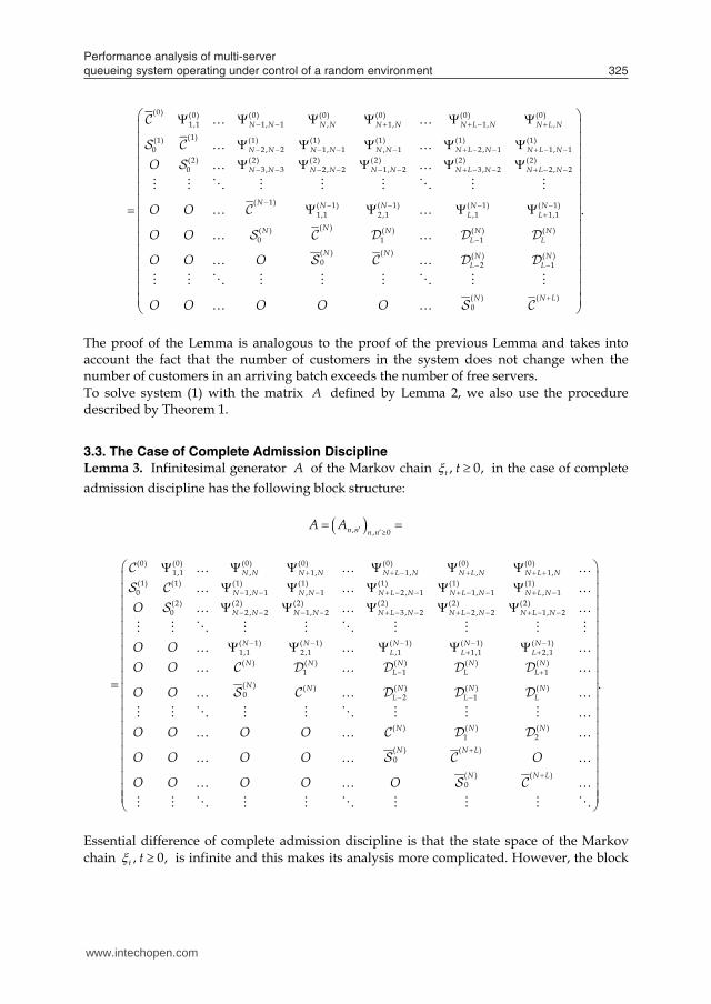
3.3. The Case of Complete Admission Discipline Lemma 3. Infinitesimal generator A of the Markov chain , 0,t t in the case of complete admission discipline has the following block structure: , , 0n n n n

A A

(0) (0) (0) (0) (0) (0) (0)1,1 , 1, 1, , 1,

(1) (1) (1) (1) (1) (1) (1)0 1, 1 , 1 2 , 1 1, 1 , 1

(2) (2) (2) (2) (2) (2)0 2 , 2 1, 2 3, 2 2 , 2 1, 2

N N N N N L N N L N N L N

N N N N N L N N L N N L N

N N N N N L N N L N N L NO

( 1) ( 1) ( 1) ( 1) ( 1)1,1 2 ,1 ,1 1,1 2 ,1( ) ( ) ( ) ( ) ( )

1 1 1( ) ( ) ( ) ( ) ( )0 2 1

( ) ( ) ( )1 2

( ) ( )0

( ) ( )0

N N N N NL L L

N N N N NL L L

N N N N NL L L

N N N

N N L

N N L

O OO O

O O

O O O O

O O O O O

O O O O O

.

Essential difference of complete admission discipline is that the state space of the Markov chain , 0,t t is infinite and this makes its analysis more complicated. However, the block

www.intechopen.com

Performance analysis of multi-server queueing system operating under control of a random environment 325

customers and occupying m servers conditional the number of busy servers is .k The entries of the matrix ( )

0k define intensity of transitions, which are accompanied by a

departure of a customer, conditional the number of busy servers is .k To solve system (1) with the matrix A defined by Lemma 1, we use the effective numerically stable procedure developed in [2] that exploits the special structure of the matrix A (it is upper block Hessenberg) and probabilistic meaning of the unknown vector

.p This procedure is given by the following statement.

Theorem 1. In case of partial admission, the stationary probability vectors , 0, ,i i N Lp are computed as follows:

0 , 1, ,l lF l N Lp p where the matrices lF are calculated recurrently:

1 10, , ,

1, 1, 1,

l

l i l l ll ii

F A F A A l N L

1 10, , ,

1,

N L

N L N L i i N L N L N Li

F A F A A

the matrices ,I N LA are calculated from the backward recursions:

, , , 0, ,I N L i N LA A i N L

, , 1, , 0, , 1, 2, ,0,i l i li l lA A A G i l l N L N L

the matrices , 0, 1,iG i N L are calculated from the backward recursion:

11

1, 1 1, 1 1 1 1,1

,N L i

i i i i i l i l i l i i il

G A A G G G A

1, 2, ,0,i N L N L

the vector 0p is calculated as the unique solution to the following system of linear algebraic equations:

0,00 0

10, 1.

N L

ll

A Fp p e e

3.2. The Case of Complete Rejection Discipline Lemma 2. Infinitesimal generator A of the Markov chain , 0,t t in the case of complete rejection discipline has the following block structure: , , 0 ,n n n n N L

A A

(0) (0) (0) (0) (0) (0) (0)1,1 1, 1 , 1, 1, ,(1)(1) (1) (1) (1) (1) (1)

0 2 , 2 1, 1 , 1 2 , 1 1, 1(2) (2) (2) (2) (2) (2)0 3, 3 2 , 2 1, 2 3, 2 2 , 2

N N N N N N N L N N L N

N N N N N N N L N N L N

N N N N N N N L N N L NO

( 1) ( 1) ( 1) ( 1) ( 1)1,1 2 ,1 ,1 1,1( )( ) ( ) ( ) ( )

0 1 1( ) ( ) ( ) ( )0 2 1

( ) ( )0

.N N N N N

L LNN N N N

L LN N N N

L L

N N L

O O

O O

O O O

O O O O O

The proof of the Lemma is analogous to the proof of the previous Lemma and takes into account the fact that the number of customers in the system does not change when the number of customers in an arriving batch exceeds the number of free servers. To solve system (1) with the matrix A defined by Lemma 2, we also use the procedure described by Theorem 1.

3.3. The Case of Complete Admission Discipline Lemma 3. Infinitesimal generator A of the Markov chain , 0,t t in the case of complete admission discipline has the following block structure: , , 0n n n n

A A

(0) (0) (0) (0) (0) (0) (0)1,1 , 1, 1, , 1,

(1) (1) (1) (1) (1) (1) (1)0 1, 1 , 1 2 , 1 1, 1 , 1

(2) (2) (2) (2) (2) (2)0 2 , 2 1, 2 3, 2 2 , 2 1, 2

N N N N N L N N L N N L N

N N N N N L N N L N N L N

N N N N N L N N L N N L NO

( 1) ( 1) ( 1) ( 1) ( 1)1,1 2 ,1 ,1 1,1 2 ,1( ) ( ) ( ) ( ) ( )

1 1 1( ) ( ) ( ) ( ) ( )0 2 1

( ) ( ) ( )1 2

( ) ( )0

( ) ( )0

N N N N NL L L

N N N N NL L L

N N N N NL L L

N N N

N N L

N N L

O OO O

O O

O O O O

O O O O O

O O O O O

.

Essential difference of complete admission discipline is that the state space of the Markov chain , 0,t t is infinite and this makes its analysis more complicated. However, the block

www.intechopen.com

Trends in Telecommunications Technologies326

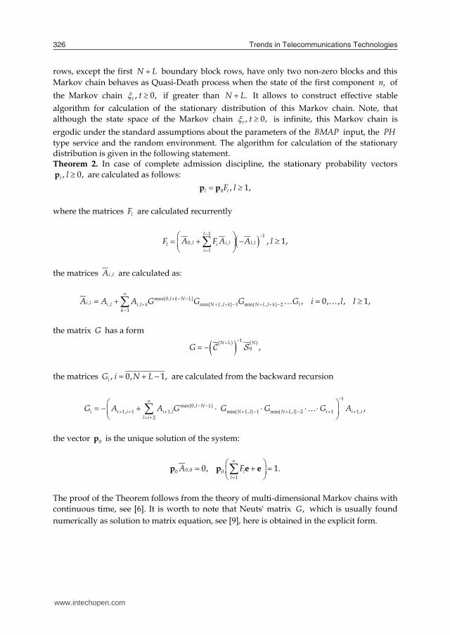
rows, except the first N L boundary block rows, have only two non-zero blocks and this Markov chain behaves as Quasi-Death process when the state of the first component tn of the Markov chain , 0,t t if greater than .N L It allows to construct effective stable algorithm for calculation of the stationary distribution of this Markov chain. Note, that although the state space of the Markov chain , 0,t t is infinite, this Markov chain is ergodic under the standard assumptions about the parameters of the BMAP input, the PH type service and the random environment. The algorithm for calculation of the stationary distribution is given in the following statement. Theorem 2. In case of complete admission discipline, the stationary probability vectors

, 0,l lp are calculated as follows: 0 , 1,l lF lp p

where the matrices lF are calculated recurrently

1 10, , ,

1, 1,

l

l i l l ll ii

F A F A A l

the matrices ,i IA are calculated as:

max{0 , }

, , , min{ , } 1 min{ , } 21

, 0, , , 1,l k N Li l i l i l k N L l k N L l k l

kA A A G G G G i l l

the matrix G has a form 1( ) ( )

0 ,N L N

G

the matrices , 0, 1,iG i N L are calculated from the backward recursion

1max{0 , }

1, 1 1, min{ , } 1 min{ , } 2 1 1,2

,l N Li i i i l N L l N L l i i i

l iG A A G G G G A

the vector 0p is the unique solution of the system:

0,00 0

10, 1.l

lA Fp p e e

The proof of the Theorem follows from the theory of multi-dimensional Markov chains with continuous time, see [6]. It is worth to note that Neuts' matrix ,G which is usually found numerically as solution to matrix equation, see [9], here is obtained in the explicit form.

3.4. The Case of an Infinite Size of a Buffer =L The system under consideration in this section has an infinite waiting space. If an arriving batch of customers sees idle servers, a part of the batch corresponding to the number of free servers occupy these servers while the rest of the batch joins the queue. If the system has all servers being busy at a batch arrival epoch, all customer of the batch go to the queue. Lemma 3. Infinitesimal generator A of the Markov chain , 0,t t has the following block structure:

, , 0n n n nA A (2)

(0) (0) (0) (0) (0) (0) (0)1,1 2 ,2 1, 1 , 1, 2 ,

(1) (1) (1) (1) (1) (1) (1)0 1,1 2 , 2 1, 1 , 1 1, 1

(2) (2) (2) (2) (2) (2)0 3, 3 2 , 2 1, 2 , 2

( 1) ( 1)1,1

N N N N N N N N

N N N N N N N N

N N N N N N N N

N N

O

O O O

( 1) ( 1)2 ,1 3,1

( ) ( ) ( ) ( )0 1 2

( ) ( ) ( )0 1

( ) ( )0

.N N

N N N N

N N N

N N

O O O

O O O O

O O O O O

In what follows we perform the steady state analysis of the Markov chain having generator of form (2). To this end, we use the results for continuous time multi-dimensional Markov chain ( QTMC ) presented in [6]. Theorem 3. The necessary and sufficient condition for existence of the Markov chain , 0,t t stationary distribution is the fulfillment of the inequality

/ 1, (3) where

'1 1( ) ,zD zx e (4)

( )2 0 , 1, ,

Nrdiag r Rx S e

the vectors , 1,2,n nx are the unique solutions to the following systems of linear algebraic equations:

1 1(1) , 1,WQ I Dx 0 x e (5)

( ) ( ) ( )2 0 2, 1, , 1.N

Nr r rMQ I diag S r Rx S 0 x e (6)

Proof. Using the results of [6], we directly obtain the desired condition in the form of inequality

www.intechopen.com

Performance analysis of multi-server queueing system operating under control of a random environment 327

rows, except the first N L boundary block rows, have only two non-zero blocks and this Markov chain behaves as Quasi-Death process when the state of the first component tn of the Markov chain , 0,t t if greater than .N L It allows to construct effective stable algorithm for calculation of the stationary distribution of this Markov chain. Note, that although the state space of the Markov chain , 0,t t is infinite, this Markov chain is ergodic under the standard assumptions about the parameters of the BMAP input, the PH type service and the random environment. The algorithm for calculation of the stationary distribution is given in the following statement. Theorem 2. In case of complete admission discipline, the stationary probability vectors

, 0,l lp are calculated as follows: 0 , 1,l lF lp p

where the matrices lF are calculated recurrently

1 10, , ,

1, 1,

l

l i l l ll ii

F A F A A l

the matrices ,i IA are calculated as:

max{0 , }

, , , min{ , } 1 min{ , } 21

, 0, , , 1,l k N Li l i l i l k N L l k N L l k l

kA A A G G G G i l l

the matrix G has a form 1( ) ( )

0 ,N L N

G

the matrices , 0, 1,iG i N L are calculated from the backward recursion

1max{0 , }

1, 1 1, min{ , } 1 min{ , } 2 1 1,2

,l N Li i i i l N L l N L l i i i

l iG A A G G G G A

the vector 0p is the unique solution of the system:

0,00 0

10, 1.l

lA Fp p e e

The proof of the Theorem follows from the theory of multi-dimensional Markov chains with continuous time, see [6]. It is worth to note that Neuts' matrix ,G which is usually found numerically as solution to matrix equation, see [9], here is obtained in the explicit form.

3.4. The Case of an Infinite Size of a Buffer =L The system under consideration in this section has an infinite waiting space. If an arriving batch of customers sees idle servers, a part of the batch corresponding to the number of free servers occupy these servers while the rest of the batch joins the queue. If the system has all servers being busy at a batch arrival epoch, all customer of the batch go to the queue. Lemma 3. Infinitesimal generator A of the Markov chain , 0,t t has the following block structure:

, , 0n n n nA A (2)

(0) (0) (0) (0) (0) (0) (0)1,1 2 ,2 1, 1 , 1, 2 ,

(1) (1) (1) (1) (1) (1) (1)0 1,1 2 , 2 1, 1 , 1 1, 1

(2) (2) (2) (2) (2) (2)0 3, 3 2 , 2 1, 2 , 2

( 1) ( 1)1,1

N N N N N N N N

N N N N N N N N

N N N N N N N N

N N

O

O O O

( 1) ( 1)2 ,1 3,1

( ) ( ) ( ) ( )0 1 2

( ) ( ) ( )0 1

( ) ( )0

.N N

N N N N

N N N

N N

O O O

O O O O

O O O O O

In what follows we perform the steady state analysis of the Markov chain having generator of form (2). To this end, we use the results for continuous time multi-dimensional Markov chain ( QTMC ) presented in [6]. Theorem 3. The necessary and sufficient condition for existence of the Markov chain , 0,t t stationary distribution is the fulfillment of the inequality

/ 1, (3) where

'1 1( ) ,zD zx e (4)

( )2 0 , 1, ,

Nrdiag r Rx S e

the vectors , 1,2,n nx are the unique solutions to the following systems of linear algebraic equations:

1 1(1) , 1,WQ I Dx 0 x e (5)

( ) ( ) ( )2 0 2, 1, , 1.N

Nr r rMQ I diag S r Rx S 0 x e (6)

Proof. Using the results of [6], we directly obtain the desired condition in the form of inequality

www.intechopen.com

Trends in Telecommunications Technologies328

( ) ( )

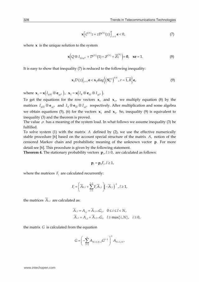
1( ) 0,N N

zz z zx e (7)

where x is the unique solution to the system

( )( ) ( )0(1) , 1.N

NN NWMQ Ix 0 xe (8)

It is easy to show that inequality (7) is reduced to the following inequality:

( )'

1 1 2 0( ) , 1, ,Nr

zD z diag r Rx e x S e (9)

where 1 ,NRW MIx x e 2 .NR W MI Ix x e

To get the equations for the row vectors 1x and 2 ,x we multiply equation (8) by the matrices NRW MI e and NR W MI Ie respectively. After multiplication and some algebra we obtain equations (5), (6) for the vectors 1x and 2 .x So, inequality (9) is equivalent to inequality (3) and the theorem is proved. The value has a meaning of the system load. In what follows we assume inequality (3) be fulfilled. To solve system (1) with the matrix A defined by (2), we use the effective numerically stable procedure [6] based on the account special structure of the matrix ,A notion of the censored Markov chain and probabilistic meaning of the unknown vector .p For more detail see [6]. This procedure is given by the following statement. Theorem 4. The stationary probability vectors , 0,l lp are calculated as follows:

0 , 1,l lF lp p

where the matrices lF are calculated recurrently:

1 10, , ,

1, 1,

l

l i l l ll ii

F A F A A l

the matrices ,i IA are calculated as:

, , 1, , 0 ,i l i li l lA A A G i l N

, , 1, , max , , 0,i l i li lA A A G l i N i

the matrix G is calculated from the equation

1

11, 1,

1,l

N N l N Nl

G A G A

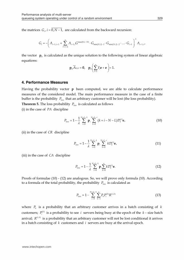
the matrices , 0, 1,iG i N are calculated from the backward recursion:

1max{0 , }

1, 1 1, min{ , } 1 min{ , } 2 1 1,2

,l Ni i i i l N l N l i i i

l iG A A G G G G A

the vector 0p is calculated as the unique solution to the following system of linear algebraic equations:

0,00 0

1, 1.l

lA Fp 0 p e e

4. Performance Measures

Having the probability vector p been computed, we are able to calculate performance measures of the considered model. The main performance measure in the case of a finite buffer is the probability lossP that an arbitrary customer will be lost (the loss probability). Theorem 5. The loss probability lossP is calculated as follows (i) in the case of PA discipline

1

( )

0 0

11 ( ) ,N L N L i

iloss i k

i kP k i N Lp e (10)

(ii) in the case of CR discipline

1

( )

0 0

11 ,N L N L i

iloss i k

i kP kp e (11)

(iii) in the case of CA discipline

1

( )

0 0

11 .N L

iloss i k

i kP kp e (12)

Proofs of formulae (10) - (12) are analogous. So, we will prove only formula (10). According to a formula of the total probability, the probability lossP is calculated as

1

( ) ( , )

0 11

N Lk i k

loss k ii k

P P P R (13)

where kP is a probability that an arbitrary customer arrives in a batch consisting of k customers; ( )k

iP is a probability to see i servers being busy at the epoch of the k size batch arrival; ( , )i kR is a probability that an arbitrary customer will not be lost conditional it arrives in a batch consisting of k customers and i servers are busy at the arrival epoch.

www.intechopen.com

Performance analysis of multi-server queueing system operating under control of a random environment 329

( ) ( )

1( ) 0,N N

zz z zx e (7)

where x is the unique solution to the system

( )( ) ( )0(1) , 1.N

NN NWMQ Ix 0 xe (8)

It is easy to show that inequality (7) is reduced to the following inequality:

( )'

1 1 2 0( ) , 1, ,Nr

zD z diag r Rx e x S e (9)

where 1 ,NRW MIx x e 2 .NR W MI Ix x e

To get the equations for the row vectors 1x and 2 ,x we multiply equation (8) by the matrices NRW MI e and NR W MI Ie respectively. After multiplication and some algebra we obtain equations (5), (6) for the vectors 1x and 2 .x So, inequality (9) is equivalent to inequality (3) and the theorem is proved. The value has a meaning of the system load. In what follows we assume inequality (3) be fulfilled. To solve system (1) with the matrix A defined by (2), we use the effective numerically stable procedure [6] based on the account special structure of the matrix ,A notion of the censored Markov chain and probabilistic meaning of the unknown vector .p For more detail see [6]. This procedure is given by the following statement. Theorem 4. The stationary probability vectors , 0,l lp are calculated as follows:

0 , 1,l lF lp p

where the matrices lF are calculated recurrently:

1 10, , ,

1, 1,

l

l i l l ll ii

F A F A A l

the matrices ,i IA are calculated as:

, , 1, , 0 ,i l i li l lA A A G i l N

, , 1, , max , , 0,i l i li lA A A G l i N i

the matrix G is calculated from the equation

1

11, 1,

1,l

N N l N Nl

G A G A

the matrices , 0, 1,iG i N are calculated from the backward recursion:

1max{0 , }

1, 1 1, min{ , } 1 min{ , } 2 1 1,2

,l Ni i i i l N l N l i i i

l iG A A G G G G A

the vector 0p is calculated as the unique solution to the following system of linear algebraic equations:

0,00 0

1, 1.l

lA Fp 0 p e e

4. Performance Measures

Having the probability vector p been computed, we are able to calculate performance measures of the considered model. The main performance measure in the case of a finite buffer is the probability lossP that an arbitrary customer will be lost (the loss probability). Theorem 5. The loss probability lossP is calculated as follows (i) in the case of PA discipline

1

( )

0 0

11 ( ) ,N L N L i

iloss i k

i kP k i N Lp e (10)

(ii) in the case of CR discipline

1

( )

0 0

11 ,N L N L i

iloss i k

i kP kp e (11)

(iii) in the case of CA discipline

1

( )

0 0

11 .N L

iloss i k

i kP kp e (12)

Proofs of formulae (10) - (12) are analogous. So, we will prove only formula (10). According to a formula of the total probability, the probability lossP is calculated as

1

( ) ( , )

0 11

N Lk i k

loss k ii k

P P P R (13)

where kP is a probability that an arbitrary customer arrives in a batch consisting of k customers; ( )k

iP is a probability to see i servers being busy at the epoch of the k size batch arrival; ( , )i kR is a probability that an arbitrary customer will not be lost conditional it arrives in a batch consisting of k customers and i servers are busy at the arrival epoch.

www.intechopen.com

Trends in Telecommunications Technologies330

It can be shown that

( )( )

(0)1

, 0, 1, 1,i

k i ki

k

P i N L kp ex e

(14)

(0) (0)

1 1'

1 1

, 1,( )

k kk

z

kP k kD zx e x e

x e (15)

( , )1, ,

, , 0, 1.i k

k N L iR N L i k N L i i N L

k (16)

By substituting (14)-(16) into (13) after some algebra we get (10). Some performance measures for the case L are presented below.

• The probability to see i customers in the system

, 0;i ip ip e

• The mean number of customers in the system

0;queue i

iL ip e

• The probability to see n busy servers

, 0, 1, ;n n N n

n Np n N pp e p e

• The mean number of busy servers

1;

N

busy n nn n N

N n Np e p e

• The mean number idleN of idle servers

;idle busyN N N

•The vector ˆ np whose ( 1) 1W r -th entry is the joint probability to see n

busy servers, the random environment in the state r and the process t in the state

ˆ ˆ, 0, 1, ;n nn n N nRW RWM M

n NI n N Ip p e p p e

•The vector of conditional means of the number of busy servers under the fixed states of the random environment

1

1

ˆmin , , 1, ;nn R rWn

n N I diag q r Rn p e

•The vector ( )( )a np whose ( 1) 1W r -th entry is the joint probability that

an arbitrary arriving call sees n busy servers and the random environment in the state r and the state of the process t becomes after the arrival epoch

( ) 1 '

1ˆ( ) ( ) , 0, ;an zn D z n Np p

• The probability ( )( )ap n that an arbitrary arriving call sees n busy servers

( ) ( )( ) ( ) , 0, ;a ap n n n Np e

•The vector ( )( )ab np whose ( 1) 1W r -th entry is the joint probability that

an arbitrary arriving batch of size k sees n busy servers and the random environment in the state r and the state of the process t becomes after the arrival epoch

( ) ( )1 ˆ( , ) , 1, , 0, , 1,a rb b n kk n diag D r R n N kp p

where (1) (0) ;b D Dx e

• The probability ( )( , )abp k n that an arbitrary arriving batch of size k sees n busy

servers ( ) ( )( , ) ( , ) , 0, , 1;a a

b bp k n k n n N kp e

•The vector ( )( )ab np whose ( 1) 1W r -th entry is the joint probability that

an arbitrary arriving batch sees n busy servers and the random environment in the state r and the state of the process t becomes after the arrival epoch

( ) 1 ˆ( ) (1) (0) , 0, ;ab b nn D D n Np p

• The probability ( )( )a

bp n that an arbitrary arriving batch sees n busy servers

( ) ( )( ) ( ) , 0, ;a ab bp n n n Np e

•The probability immP that an arbitrary customer will enter the service

immediately upon arrival (without visiting a buffer)

www.intechopen.com

Performance analysis of multi-server queueing system operating under control of a random environment 331

It can be shown that

( )( )

(0)1

, 0, 1, 1,i

k i ki

k

P i N L kp ex e

(14)

(0) (0)

1 1'

1 1

, 1,( )

k kk

z

kP k kD zx e x e

x e (15)

( , )1, ,

, , 0, 1.i k

k N L iR N L i k N L i i N L

k (16)

By substituting (14)-(16) into (13) after some algebra we get (10). Some performance measures for the case L are presented below.

• The probability to see i customers in the system

, 0;i ip ip e

• The mean number of customers in the system

0;queue i

iL ip e

• The probability to see n busy servers

, 0, 1, ;n n N n

n Np n N pp e p e

• The mean number of busy servers

1;

N

busy n nn n N

N n Np e p e

• The mean number idleN of idle servers

;idle busyN N N

•The vector ˆ np whose ( 1) 1W r -th entry is the joint probability to see n

busy servers, the random environment in the state r and the process t in the state

ˆ ˆ, 0, 1, ;n nn n N nRW RWM M

n NI n N Ip p e p p e

•The vector of conditional means of the number of busy servers under the fixed states of the random environment

1

1

ˆmin , , 1, ;nn R rWn

n N I diag q r Rn p e

•The vector ( )( )a np whose ( 1) 1W r -th entry is the joint probability that

an arbitrary arriving call sees n busy servers and the random environment in the state r and the state of the process t becomes after the arrival epoch

( ) 1 '

1ˆ( ) ( ) , 0, ;an zn D z n Np p

• The probability ( )( )ap n that an arbitrary arriving call sees n busy servers

( ) ( )( ) ( ) , 0, ;a ap n n n Np e

•The vector ( )( )ab np whose ( 1) 1W r -th entry is the joint probability that

an arbitrary arriving batch of size k sees n busy servers and the random environment in the state r and the state of the process t becomes after the arrival epoch

( ) ( )1 ˆ( , ) , 1, , 0, , 1,a rb b n kk n diag D r R n N kp p

where (1) (0) ;b D Dx e

• The probability ( )( , )abp k n that an arbitrary arriving batch of size k sees n busy

servers ( ) ( )( , ) ( , ) , 0, , 1;a a

b bp k n k n n N kp e

•The vector ( )( )ab np whose ( 1) 1W r -th entry is the joint probability that

an arbitrary arriving batch sees n busy servers and the random environment in the state r and the state of the process t becomes after the arrival epoch

( ) 1 ˆ( ) (1) (0) , 0, ;ab b nn D D n Np p

• The probability ( )( )a

bp n that an arbitrary arriving batch sees n busy servers

( ) ( )( ) ( ) , 0, ;a ab bp n n n Np e

•The probability immP that an arbitrary customer will enter the service

immediately upon arrival (without visiting a buffer)

www.intechopen.com

Trends in Telecommunications Technologies332

1( )1

0 0( ) .

N N ii

imm i ki k

P k i Np e

5. Actual Sojourn Time

Let ( ), 0,a s Re s be the Laplace-Stieltjes transform ( LST ) of the sojourn time distribution

and a be the mean sojourn time of the arbitrary customer in the system. Theorem 6. The Laplace-Stieltjes transform ( )a s is calculated as follows

1

( )

0 1

1( ) min , i

Ni

a i k R Wmi k

s k N i Ip e (17)

(min{ , }) (max{0 , })

0 max{1, 1} max{1, 1}( ) ( ) ,N

ki N li N N i

i k R RMi k N i l N i

s I sp e e

where 1( ) ( )0( ) , 1, ( ) , 1, ,r r

Ms diag r R sI Q I diag r RS

1

( ) ( ) ( )0( ) , 1, , 1, ,N

N Nr r rMs sI Q I diag S r R diag r RS

( ) ( ) , 1, , 0, ,N n

nn rW Mdiag I r R n Ne

( ) , 1, .rdiag S r R

Proof. We derive the expression for the LST ( )a s by means of the method of collective marks (method of additional event, method of catastrophes) for references see, e.g. [3], [11]. To this end, we interpret the variable s as the intensity of some virtual stationary Poisson flow of catastrophes. So, ( )a s has the meaning of probability that no one catastrophe arrives during the sojourn time of an arbitrary customer. Then, the proof of the theorem follows from the formula of total probability if we analyze the states of the system at an arbitrary customer arrival epoch and take into account the probabilistic meaning of the involved matrices. The matrix ( )s is the matrix LST of an arbitrary customer service time distribution. It is the R -size square matrix whose ( , )r r entry is a probability that during the service time of a customer a catastrophe does not arrive and the process 0,tr t transits

from the state r to the state , , 1, .r r r R It is defined by the formula:

( )( { , 1, })( ) ( )

00

( ) , 1, e e , 1, .r

MQ I diag S r R tr rsts diag r R dt diag r RS

Analogously, the entries of the matrix LST ( )s are the probabilities of no catastrophe arrival and corresponding transitions of the process (1) ( ){ , , , }, 0,N

t t tr m m t during the time

interval from an arbitrary moment when all N servers are busy till the first epoch when one of these servers finishes the service of a customer. This matrix is defined by the formula:

( )( {( ) , 1, }) ( ) ( )

00

( ) e e , 1, .r N

NMNQ I diag S r R t r rsts dt diag r RS

Theorem 7. The mean sojourn time a of an arbitrary customer in the system is calculated by

1(min{ , }) (max{0 , })

0 max{1, 1} max{1, 1} 0

1 (0) (0) N

k i l Nmi N N i

a i k R Mi k N i l N i m

Ip e

1

( )

0 1min{ , } (0)i

Ni

i k R WMi k

k N i Ip e (18)

(min{ , }) (max{0, })

0 max{1, 1} max{1, 1}(0) (0)

ki N li N N i

i k R RMi k N i l N i

Ip e e

where 2( ) ( )0(0) , 1, , 1, ,r r

Mdiag r R Q I diag r RS

2

( ) ( ) ( )0(0) , 1, , 1, .N

N Nr r rMQ I diag S r R diag r RS

Proof. To get expression (18) for a we differentiate (17) at the point 0s and use the formula '

(0).a a

6. Numerical Examples

The goal of the numerical experiments is to demonstrate the feasibility of the proposed algorithms for computing the stationary distributions of the number of customers and the sojourn time in the system and to give some insight into behavior of the considered queueing systems. In particular, the following issues are addressed:

• Comparison of the mean sojourn time of an arbitrary customer and the probability of immediate access to the servers in the systems with varying traffic intensities and different coefficients of correlation in the BMAP s (experiment #1 );

• Comparison of the mean sojourn time of an arbitrary customer and the probability of immediate access to the servers in the original system in a RE and in more simple queueing systems for different system loads (experiments #2 );

• Demonstration of possible positive effect of redistribution of traffic between the peak traffic periods and normal traffic periods (experiment #3 );

• Comparison of the exact value of performance measures of the system in a RE and their simple engineering approximations in cases of slowly and quickly varying RE (experiment #4 );

• Investigation of the rate of convergence of the mean sojourn time and the probability of immediate access in the system with the finite buffer to corresponding

www.intechopen.com

Performance analysis of multi-server queueing system operating under control of a random environment 333

1( )1

0 0( ) .

N N ii

imm i ki k

P k i Np e

5. Actual Sojourn Time

Let ( ), 0,a s Re s be the Laplace-Stieltjes transform ( LST ) of the sojourn time distribution

and a be the mean sojourn time of the arbitrary customer in the system. Theorem 6. The Laplace-Stieltjes transform ( )a s is calculated as follows

1

( )

0 1

1( ) min , i

Ni

a i k R Wmi k

s k N i Ip e (17)

(min{ , }) (max{0 , })

0 max{1, 1} max{1, 1}( ) ( ) ,N

ki N li N N i

i k R RMi k N i l N i

s I sp e e

where 1( ) ( )0( ) , 1, ( ) , 1, ,r r

Ms diag r R sI Q I diag r RS

1

( ) ( ) ( )0( ) , 1, , 1, ,N

N Nr r rMs sI Q I diag S r R diag r RS

( ) ( ) , 1, , 0, ,N n

nn rW Mdiag I r R n Ne

( ) , 1, .rdiag S r R

Proof. We derive the expression for the LST ( )a s by means of the method of collective marks (method of additional event, method of catastrophes) for references see, e.g. [3], [11]. To this end, we interpret the variable s as the intensity of some virtual stationary Poisson flow of catastrophes. So, ( )a s has the meaning of probability that no one catastrophe arrives during the sojourn time of an arbitrary customer. Then, the proof of the theorem follows from the formula of total probability if we analyze the states of the system at an arbitrary customer arrival epoch and take into account the probabilistic meaning of the involved matrices. The matrix ( )s is the matrix LST of an arbitrary customer service time distribution. It is the R -size square matrix whose ( , )r r entry is a probability that during the service time of a customer a catastrophe does not arrive and the process 0,tr t transits

from the state r to the state , , 1, .r r r R It is defined by the formula:

( )( { , 1, })( ) ( )

00

( ) , 1, e e , 1, .r

MQ I diag S r R tr rsts diag r R dt diag r RS

Analogously, the entries of the matrix LST ( )s are the probabilities of no catastrophe arrival and corresponding transitions of the process (1) ( ){ , , , }, 0,N

t t tr m m t during the time

interval from an arbitrary moment when all N servers are busy till the first epoch when one of these servers finishes the service of a customer. This matrix is defined by the formula:

( )( {( ) , 1, }) ( ) ( )

00

( ) e e , 1, .r N

NMNQ I diag S r R t r rsts dt diag r RS

Theorem 7. The mean sojourn time a of an arbitrary customer in the system is calculated by

1(min{ , }) (max{0 , })

0 max{1, 1} max{1, 1} 0

1 (0) (0) N

k i l Nmi N N i

a i k R Mi k N i l N i m

Ip e

1

( )

0 1min{ , } (0)i

Ni

i k R WMi k

k N i Ip e (18)

(min{ , }) (max{0, })

0 max{1, 1} max{1, 1}(0) (0)

ki N li N N i

i k R RMi k N i l N i

Ip e e

where 2( ) ( )0(0) , 1, , 1, ,r r

Mdiag r R Q I diag r RS

2

( ) ( ) ( )0(0) , 1, , 1, .N

N Nr r rMQ I diag S r R diag r RS

Proof. To get expression (18) for a we differentiate (17) at the point 0s and use the formula '

(0).a a

6. Numerical Examples

The goal of the numerical experiments is to demonstrate the feasibility of the proposed algorithms for computing the stationary distributions of the number of customers and the sojourn time in the system and to give some insight into behavior of the considered queueing systems. In particular, the following issues are addressed:

• Comparison of the mean sojourn time of an arbitrary customer and the probability of immediate access to the servers in the systems with varying traffic intensities and different coefficients of correlation in the BMAP s (experiment #1 );

• Comparison of the mean sojourn time of an arbitrary customer and the probability of immediate access to the servers in the original system in a RE and in more simple queueing systems for different system loads (experiments #2 );

• Demonstration of possible positive effect of redistribution of traffic between the peak traffic periods and normal traffic periods (experiment #3 );

• Comparison of the exact value of performance measures of the system in a RE and their simple engineering approximations in cases of slowly and quickly varying RE (experiment #4 );

• Investigation of the rate of convergence of the mean sojourn time and the probability of immediate access in the system with the finite buffer to corresponding

www.intechopen.com

Trends in Telecommunications Technologies334

performance measures of the system with an infinite buffer when the buffer size increases (experiment #5 );

• Demonstration of the possibility to apply the presented results for optimization of the number of servers in the system (experiment #6 ).

In numerical examples, we consider the systems operating in the RE which has two states

( 2R ). The generator of the random environment is

5 5.

15 15Q The stationary

distribution of the RE states is defined by the vector 0.75, 0.25 .q The number of servers is 3.N In the presented examples, we will use several different MAP s and BMAP s for description of the arrival process and two PH type distributions for description of the service processes under the fixed value of the .RE For the use in the sequel, let us define these processes. We consider four arrival processes , 1,4.rMAP r rMAP is defined by the matrices ( )

0 ,rD

( )1 , 1,4,rD r where

(1) (1)0 1

3.9 0.15 0.15 3.5 0.08 0.020.13 0.6 0.1 , 0.03 0.3 0.04 ;0.15 0.14 0.5 0.02 0.06 0.13

D D

(2) (2)0 1

6.4 0.1 0.1 6.06 0.12 0.020.04 0.6 0.1 , 0.01 0.4 0.05 ;0.07 0.1 0.44 0.01 0.06 0.2

D D

(3) (3)0 1

2.9 0.73 0.77 0.68 0.45 0.270.87 3.06 0.53 , 0.48 1.08 0.1 ;0.85 0.5 2 0.35 0.05 0.25

D D

(4) (4)0 1

1.3 0.21 0.17 0.46 0.32 0.140.16 2.04 0.21 , 0.13 1.34 0.2 .0.01 0.16 1.3 0.02 0.01 1.1

D D

All these MAP s have fundamental rate ( ) 1.25.r The 1MAP has the squared variation

coefficient 2(1) 4varc and the coefficient of correlation of the lengths of successive inter-

arrival times (1) 0.2.corc For the rest of the MAP s, the corresponding parameters are:

2(2) 4,varc (2) 0.3;corc 2(3) 1.097,varc (3) 0.0052;corc 2(4) 1.037,varc (4) 0.0065.corc

Based on these MAP s, we construct batch flows BMAP s as follows. If the MAP is defined by the matrices ( )

0 ,rD and ( )1 , 1,4,rD r then the BMAP having the maximal size of a batch

equal to K is defined by the matrices ( )0 ,rD ( ) ( ) 1

1 (1 )/(1 ), 1, , 1, ,r r k KkD D q q q k K r R

where 0.9.q

Following this way, we construct the 1 ,BMAP 2 ,BMAP 3 ,BMAP 4BMAP flows based on the 1 ,MAP 2 ,MAP 3 ,MAP 4MAP correspondingly, with 5.K Note that the coefficients of variation and correlation of all BMAP s are the same as these coefficients for the corresponding MAP s. Fundamental rate ( )r and the mean batch size

( )rk of the BMAP s

are the following: (1) (2) (3) (4) 3.488, (1) (2) (3) (4)1.989.k k k k

The , 1,2,rPH r service processes are defined by the vectors (1) 1, 0 , (2) 0.2, 0.8 and the matrices

(1) (2)4 4 10 2

, .0 4 2 20

S S

The mean rates of service are (1) (2)2, 14. The coefficients of variation of the service

time distribution are defined by 2(1) 0.5,varc 2(2) 1.24.varc

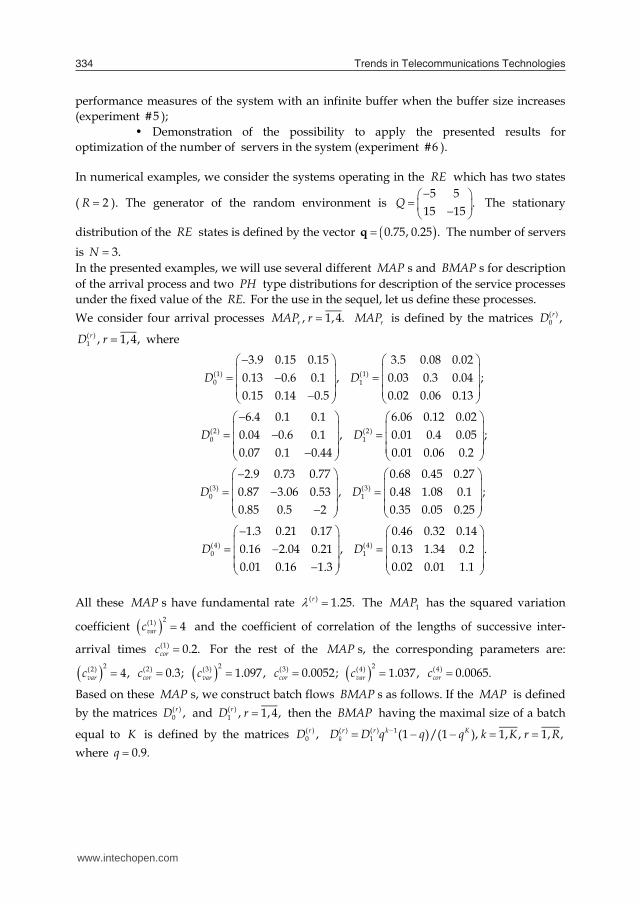
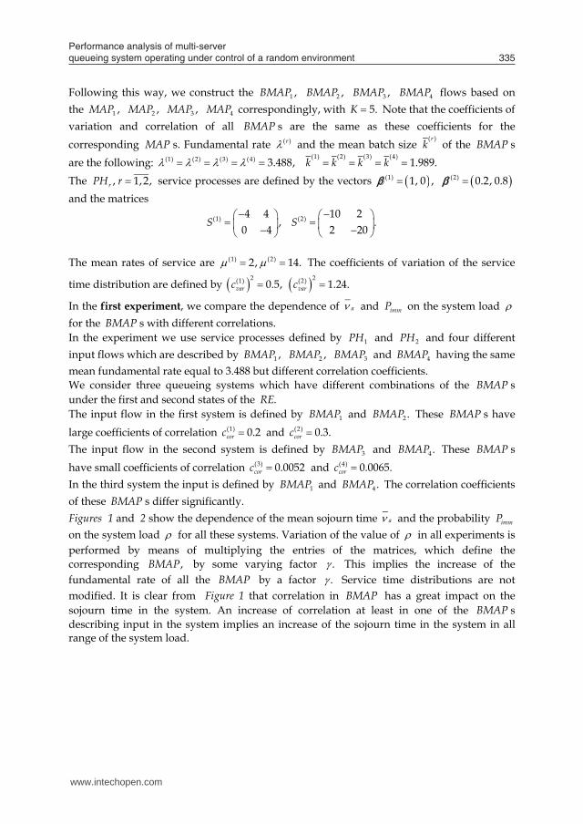
In the first experiment, we compare the dependence of a and immP on the system load for the BMAP s with different correlations. In the experiment we use service processes defined by 1PH and 2PH and four different input flows which are described by 1 ,BMAP 2 ,BMAP 3BMAP and 4BMAP having the same mean fundamental rate equal to 3.488 but different correlation coefficients. We consider three queueing systems which have different combinations of the BMAP s under the first and second states of the .RE The input flow in the first system is defined by 1BMAP and 2 .BMAP These BMAP s have large coefficients of correlation (1) 0.2corc and (2) 0.3.corc The input flow in the second system is defined by 3BMAP and 4 .BMAP These BMAP s have small coefficients of correlation (3) 0.0052corc and (4) 0.0065.corc In the third system the input is defined by 1BMAP and 4 .BMAP The correlation coefficients of these BMAP s differ significantly. Figures 1 and 2 show the dependence of the mean sojourn time a and the probability immP on the system load for all these systems. Variation of the value of in all experiments is performed by means of multiplying the entries of the matrices, which define the corresponding ,BMAP by some varying factor . This implies the increase of the fundamental rate of all the BMAP by a factor . Service time distributions are not modified. It is clear from Figure 1 that correlation in BMAP has a great impact on the sojourn time in the system. An increase of correlation at least in one of the BMAP s describing input in the system implies an increase of the sojourn time in the system in all range of the system load.

www.intechopen.com

Performance analysis of multi-server queueing system operating under control of a random environment 335

performance measures of the system with an infinite buffer when the buffer size increases (experiment #5 );

• Demonstration of the possibility to apply the presented results for optimization of the number of servers in the system (experiment #6 ).

In numerical examples, we consider the systems operating in the RE which has two states

( 2R ). The generator of the random environment is

5 5.

15 15Q The stationary

distribution of the RE states is defined by the vector 0.75, 0.25 .q The number of servers is 3.N In the presented examples, we will use several different MAP s and BMAP s for description of the arrival process and two PH type distributions for description of the service processes under the fixed value of the .RE For the use in the sequel, let us define these processes. We consider four arrival processes , 1,4.rMAP r rMAP is defined by the matrices ( )

0 ,rD

( )1 , 1,4,rD r where

(1) (1)0 1

3.9 0.15 0.15 3.5 0.08 0.020.13 0.6 0.1 , 0.03 0.3 0.04 ;0.15 0.14 0.5 0.02 0.06 0.13

D D

(2) (2)0 1

6.4 0.1 0.1 6.06 0.12 0.020.04 0.6 0.1 , 0.01 0.4 0.05 ;0.07 0.1 0.44 0.01 0.06 0.2

D D

(3) (3)0 1

2.9 0.73 0.77 0.68 0.45 0.270.87 3.06 0.53 , 0.48 1.08 0.1 ;0.85 0.5 2 0.35 0.05 0.25

D D

(4) (4)0 1

1.3 0.21 0.17 0.46 0.32 0.140.16 2.04 0.21 , 0.13 1.34 0.2 .0.01 0.16 1.3 0.02 0.01 1.1

D D

All these MAP s have fundamental rate ( ) 1.25.r The 1MAP has the squared variation

coefficient 2(1) 4varc and the coefficient of correlation of the lengths of successive inter-

arrival times (1) 0.2.corc For the rest of the MAP s, the corresponding parameters are:

2(2) 4,varc (2) 0.3;corc 2(3) 1.097,varc (3) 0.0052;corc 2(4) 1.037,varc (4) 0.0065.corc

Based on these MAP s, we construct batch flows BMAP s as follows. If the MAP is defined by the matrices ( )

0 ,rD and ( )1 , 1,4,rD r then the BMAP having the maximal size of a batch

equal to K is defined by the matrices ( )0 ,rD ( ) ( ) 1

1 (1 )/(1 ), 1, , 1, ,r r k KkD D q q q k K r R

where 0.9.q

Following this way, we construct the 1 ,BMAP 2 ,BMAP 3 ,BMAP 4BMAP flows based on the 1 ,MAP 2 ,MAP 3 ,MAP 4MAP correspondingly, with 5.K Note that the coefficients of variation and correlation of all BMAP s are the same as these coefficients for the corresponding MAP s. Fundamental rate ( )r and the mean batch size

( )rk of the BMAP s

are the following: (1) (2) (3) (4) 3.488, (1) (2) (3) (4)1.989.k k k k

The , 1,2,rPH r service processes are defined by the vectors (1) 1, 0 , (2) 0.2, 0.8 and the matrices

(1) (2)4 4 10 2

, .0 4 2 20

S S

The mean rates of service are (1) (2)2, 14. The coefficients of variation of the service

time distribution are defined by 2(1) 0.5,varc 2(2) 1.24.varc

In the first experiment, we compare the dependence of a and immP on the system load for the BMAP s with different correlations. In the experiment we use service processes defined by 1PH and 2PH and four different input flows which are described by 1 ,BMAP 2 ,BMAP 3BMAP and 4BMAP having the same mean fundamental rate equal to 3.488 but different correlation coefficients. We consider three queueing systems which have different combinations of the BMAP s under the first and second states of the .RE The input flow in the first system is defined by 1BMAP and 2 .BMAP These BMAP s have large coefficients of correlation (1) 0.2corc and (2) 0.3.corc The input flow in the second system is defined by 3BMAP and 4 .BMAP These BMAP s have small coefficients of correlation (3) 0.0052corc and (4) 0.0065.corc In the third system the input is defined by 1BMAP and 4 .BMAP The correlation coefficients of these BMAP s differ significantly. Figures 1 and 2 show the dependence of the mean sojourn time a and the probability immP on the system load for all these systems. Variation of the value of in all experiments is performed by means of multiplying the entries of the matrices, which define the corresponding ,BMAP by some varying factor . This implies the increase of the fundamental rate of all the BMAP by a factor . Service time distributions are not modified. It is clear from Figure 1 that correlation in BMAP has a great impact on the sojourn time in the system. An increase of correlation at least in one of the BMAP s describing input in the system implies an increase of the sojourn time in the system in all range of the system load.

www.intechopen.com

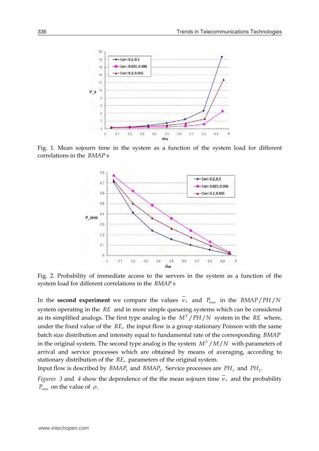
Trends in Telecommunications Technologies336

Fig. 1. Mean sojourn time in the system as a function of the system load for different correlations in the BMAP s

Fig. 2. Probability of immediate access to the servers in the system as a function of the system load for different correlations in the BMAP s

In the second experiment we compare the values a and immP in the / /BMAP PH N system operating in the RE and in more simple queueing systems which can be considered as its simplified analogs. The first type analog is the / /XM PH N system in the RE where, under the fixed value of the ,RE the input flow is a group stationary Poisson with the same batch size distribution and intensity equal to fundamental rate of the corresponding BMAP in the original system. The second type analog is the system / /XM M N with parameters of arrival and service processes which are obtained by means of averaging, according to stationary distribution of the ,RE parameters of the original system. Input flow is described by 1BMAP and 2 .BMAP Service processes are 1PH and 2 .PH

Figures 3 and 4 show the dependence of the the mean sojourn time a and the probability immP on the value of .

Fig. 3. Mean sojourn time in original system and more simple queueing systems

Fig. 4. Probability of immediate access to the servers in original system and more simple queueing systems It can be seen from Figures 3 and 4 that an approximation of the mean sojourn time and the probability that an arbitrary call reaches the server immediately by means of their values in some specially constructed more simple queueing system can be rather bad. The idea of the third experiment is the following. Let us assume that the RE has two states. One state corresponds to the peak traffic periods, the second one corresponds to the normal traffic periods. Service times during these periods are defined by 1PH and 2PH distributions. Arrivals during these periods are defined by the stationary Poisson flow with the rates 1 and 2 correspondingly and initially we assume that 1 2 . It is intuitively clear that if it is possible to redistribute the arrival processes (i.e., to reduce the arrival rate during the peak periods and to increase it correspondingly during the normal traffic periods) without changing the total average arrival rate, the mean sojourn time in the system can be reduced. In real life system such a redistribution is sometimes possible, e.g., by means of controlling tariffs during the peak traffic periods. The goal of this experiment is to show that this intuitive consideration is correct and to illustrate the effect of the redistribution.

www.intechopen.com

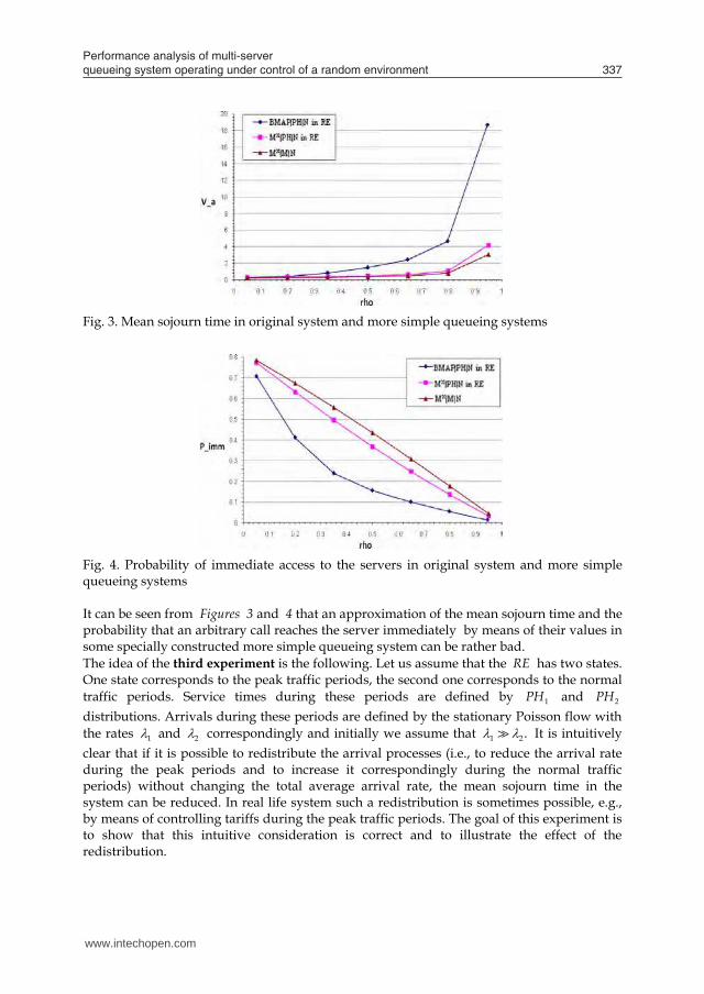
Performance analysis of multi-server queueing system operating under control of a random environment 337

Fig. 1. Mean sojourn time in the system as a function of the system load for different correlations in the BMAP s

Fig. 2. Probability of immediate access to the servers in the system as a function of the system load for different correlations in the BMAP s

In the second experiment we compare the values a and immP in the / /BMAP PH N system operating in the RE and in more simple queueing systems which can be considered as its simplified analogs. The first type analog is the / /XM PH N system in the RE where, under the fixed value of the ,RE the input flow is a group stationary Poisson with the same batch size distribution and intensity equal to fundamental rate of the corresponding BMAP in the original system. The second type analog is the system / /XM M N with parameters of arrival and service processes which are obtained by means of averaging, according to stationary distribution of the ,RE parameters of the original system. Input flow is described by 1BMAP and 2 .BMAP Service processes are 1PH and 2 .PH

Figures 3 and 4 show the dependence of the the mean sojourn time a and the probability immP on the value of .

Fig. 3. Mean sojourn time in original system and more simple queueing systems

Fig. 4. Probability of immediate access to the servers in original system and more simple queueing systems It can be seen from Figures 3 and 4 that an approximation of the mean sojourn time and the probability that an arbitrary call reaches the server immediately by means of their values in some specially constructed more simple queueing system can be rather bad. The idea of the third experiment is the following. Let us assume that the RE has two states. One state corresponds to the peak traffic periods, the second one corresponds to the normal traffic periods. Service times during these periods are defined by 1PH and 2PH distributions. Arrivals during these periods are defined by the stationary Poisson flow with the rates 1 and 2 correspondingly and initially we assume that 1 2 . It is intuitively clear that if it is possible to redistribute the arrival processes (i.e., to reduce the arrival rate during the peak periods and to increase it correspondingly during the normal traffic periods) without changing the total average arrival rate, the mean sojourn time in the system can be reduced. In real life system such a redistribution is sometimes possible, e.g., by means of controlling tariffs during the peak traffic periods. The goal of this experiment is to show that this intuitive consideration is correct and to illustrate the effect of the redistribution.

www.intechopen.com

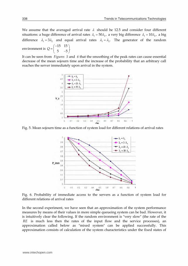
Trends in Telecommunications Technologies338

We assume that the averaged arrival rate should be 12.5 and consider four different situations: a huge difference of arrival rates 1 250 , a very big difference 1 210 , a big difference 1 23 and equal arrival rates 1 2 . The generator of the random

environment is

15 15.

5 5Q

It can be seen from Figures 5 and 6 that the smoothing of the peak rates can cause essential decrease of the mean sojourn time and the increase of the probability that an arbitrary call reaches the server immediately upon arrival in the system.

Fig. 5. Mean sojourn time as a function of system load for different relations of arrival rates

Fig. 6. Probability of immediate access to the servers as a function of system load for different relations of arrival rates

In the second experiment, we have seen that an approximation of the system performance measures by means of their values in more simple queueing system can be bad. However, it is intuitively clear the following. If the random environment is "very slow" (the rate of the RE is much less then the rates of the input flow and the service processes), an approximation called below as "mixed system" can be applied successfully. This approximation consists of calculation of the system characteristics under the fixed states of

the RE and their averaging by the RE distribution. If the random environment is "very fast", approximation called below as "mixed parameters" can be successfully applied. This approximation consists of averaging parameters of the arrival and service processes by the distribution of the RE and calculation of performance measures in / /BMAP PH N system with the averaged arrival and service rates. In the fourth experiment, we show numerically that sometimes the described approximations make sense. However, in situations when environment is neither "very slow" nor "very fast", these approximations can be very poor. We consider the RE s with

different rate which are characterized by the generators of the form

( ) 5 510 .

15 15k kQ

We vary the parameter k from -7 to 4 what corresponds to the variation of the RE rate from "very slow" to "very fast". In this and further experiments, the input flow is described by the 1BMAP and 2BMAP and the service process is defined by the 1PH and 2 .PH The results are presented in Figures 7, 8 and 9. In application of "mixed system" approximation, the averaged arrival rates under both states of the RE are equal to 3.488. The averaged service rate is equal to 2 at the first state of the RE and is equal to 14 at the second state. The mean sojourn times of an arbitrary customer at these states are equal to 3.5297 and 0.0998, respectively; the probabilities of immediate access to the servers are equal to 0.2021 and 0.81399; the mean numbers of customers in the system are equal to 12.311 and 0.3482. The averaged, according to the stationary distribution of the ,RE mean sojourn time of an arbitrary customer is equal to 2.6722 and the probability that an arbitrary arriving customer sees an idle server is equal to 0.355. In application of "mixed parameters" approximation, the averaged, according to the stationary distribution of the ,RE arrival rate is equal to 3.778 while the averaged service rate is equal to 4.0625. The value of the mean sojourn time of an arbitrary customer in the system with averaged arrival and service rates is equal to 0.7541, the probability of immediate access to the servers is equal to 0.4168, the mean number of customers in the system is equal to 2.849. Figures 7, 8 and 9 confirm the hypothesis that the first type approximation ("mixed system") is good in case of "very slow" RE and the second one ("mixed parameters") can be applied to case of "very fast" .RE But sometimes the second type approximation is not very good (see Figures 8) because it is not quite clear how to make averaging of service intensity. Simple averaging of service rates under the different states of the RE may be not correct when the load of the system is not high because there are time intervals when the system is empty and no service is provided. It is worth to note also that there is an interval for RE rate (interval 3, 0k ) where one should not use the values of the system performance measures calculated based on the considered approximating models. The use of these values can lead to the large relative error. Thus, Figures 7, 8 and 9 confirm the importance of investigation implemented in this chapter. Simple engineering approximations can lead to unsatisfactory performance evaluation and capacity planning in real world systems.

www.intechopen.com

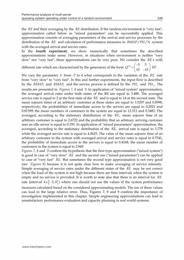
Performance analysis of multi-server queueing system operating under control of a random environment 339

We assume that the averaged arrival rate should be 12.5 and consider four different situations: a huge difference of arrival rates 1 250 , a very big difference 1 210 , a big difference 1 23 and equal arrival rates 1 2 . The generator of the random

environment is

15 15.

5 5Q

It can be seen from Figures 5 and 6 that the smoothing of the peak rates can cause essential decrease of the mean sojourn time and the increase of the probability that an arbitrary call reaches the server immediately upon arrival in the system.

Fig. 5. Mean sojourn time as a function of system load for different relations of arrival rates

Fig. 6. Probability of immediate access to the servers as a function of system load for different relations of arrival rates

In the second experiment, we have seen that an approximation of the system performance measures by means of their values in more simple queueing system can be bad. However, it is intuitively clear the following. If the random environment is "very slow" (the rate of the RE is much less then the rates of the input flow and the service processes), an approximation called below as "mixed system" can be applied successfully. This approximation consists of calculation of the system characteristics under the fixed states of

the RE and their averaging by the RE distribution. If the random environment is "very fast", approximation called below as "mixed parameters" can be successfully applied. This approximation consists of averaging parameters of the arrival and service processes by the distribution of the RE and calculation of performance measures in / /BMAP PH N system with the averaged arrival and service rates. In the fourth experiment, we show numerically that sometimes the described approximations make sense. However, in situations when environment is neither "very slow" nor "very fast", these approximations can be very poor. We consider the RE s with

different rate which are characterized by the generators of the form

( ) 5 510 .

15 15k kQ

We vary the parameter k from -7 to 4 what corresponds to the variation of the RE rate from "very slow" to "very fast". In this and further experiments, the input flow is described by the 1BMAP and 2BMAP and the service process is defined by the 1PH and 2 .PH The results are presented in Figures 7, 8 and 9. In application of "mixed system" approximation, the averaged arrival rates under both states of the RE are equal to 3.488. The averaged service rate is equal to 2 at the first state of the RE and is equal to 14 at the second state. The mean sojourn times of an arbitrary customer at these states are equal to 3.5297 and 0.0998, respectively; the probabilities of immediate access to the servers are equal to 0.2021 and 0.81399; the mean numbers of customers in the system are equal to 12.311 and 0.3482. The averaged, according to the stationary distribution of the ,RE mean sojourn time of an arbitrary customer is equal to 2.6722 and the probability that an arbitrary arriving customer sees an idle server is equal to 0.355. In application of "mixed parameters" approximation, the averaged, according to the stationary distribution of the ,RE arrival rate is equal to 3.778 while the averaged service rate is equal to 4.0625. The value of the mean sojourn time of an arbitrary customer in the system with averaged arrival and service rates is equal to 0.7541, the probability of immediate access to the servers is equal to 0.4168, the mean number of customers in the system is equal to 2.849. Figures 7, 8 and 9 confirm the hypothesis that the first type approximation ("mixed system") is good in case of "very slow" RE and the second one ("mixed parameters") can be applied to case of "very fast" .RE But sometimes the second type approximation is not very good (see Figures 8) because it is not quite clear how to make averaging of service intensity. Simple averaging of service rates under the different states of the RE may be not correct when the load of the system is not high because there are time intervals when the system is empty and no service is provided. It is worth to note also that there is an interval for RE rate (interval 3, 0k ) where one should not use the values of the system performance measures calculated based on the considered approximating models. The use of these values can lead to the large relative error. Thus, Figures 7, 8 and 9 confirm the importance of investigation implemented in this chapter. Simple engineering approximations can lead to unsatisfactory performance evaluation and capacity planning in real world systems.

www.intechopen.com

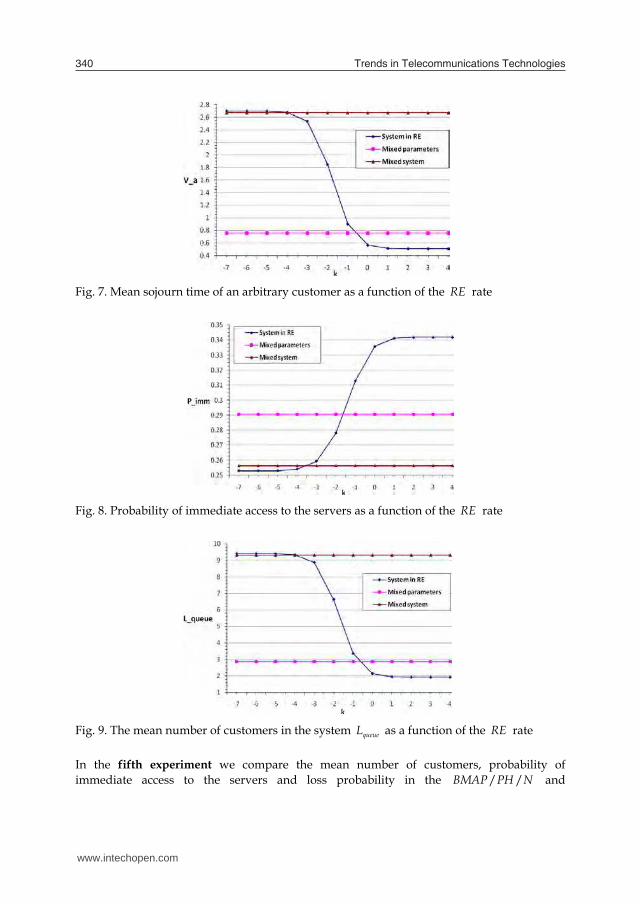
Trends in Telecommunications Technologies340

Fig. 7. Mean sojourn time of an arbitrary customer as a function of the RE rate

Fig. 8. Probability of immediate access to the servers as a function of the RE rate

Fig. 9. The mean number of customers in the system queueL as a function of the RE rate In the fifth experiment we compare the mean number of customers, probability of immediate access to the servers and loss probability in the / /BMAP PH N and

/ / /BMAP PH N L systems operating in the RE for different values L of the buffer capacity and different customers admission discipline.

Fig. 10. Mean number of customers in the system as a function of the buffer capacity L

Fig. 11. Probability of immediate access to the servers as a function of the buffer capacity L

Fig. 12. Loss probability as a function of the buffer capacity L

www.intechopen.com

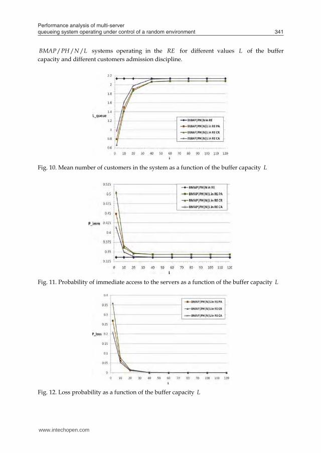
Performance analysis of multi-server queueing system operating under control of a random environment 341

Fig. 7. Mean sojourn time of an arbitrary customer as a function of the RE rate

Fig. 8. Probability of immediate access to the servers as a function of the RE rate

Fig. 9. The mean number of customers in the system queueL as a function of the RE rate In the fifth experiment we compare the mean number of customers, probability of immediate access to the servers and loss probability in the / /BMAP PH N and

/ / /BMAP PH N L systems operating in the RE for different values L of the buffer capacity and different customers admission discipline.

Fig. 10. Mean number of customers in the system as a function of the buffer capacity L

Fig. 11. Probability of immediate access to the servers as a function of the buffer capacity L

Fig. 12. Loss probability as a function of the buffer capacity L

www.intechopen.com

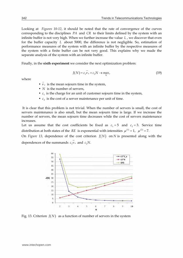
Trends in Telecommunications Technologies342

Looking at Figures 10-12, it should be noted that the rate of convergence of the curves corresponding to the disciplines PA and CR to their limits defined by the system with an infinite buffer is not very high. When we further increase the value L , we discover that even for the buffer capacity L about 5000, the difference is not negligible. So, estimation of performance measures of the system with an infinite buffer by the respective measures of the system with a finite buffer can be not very good. This explains why we made the separate analysis of the system with an infinite buffer. Finally, in the sixth experiment we consider the next optimization problem:

1 2 ,aN

J N c c N max (19)

where • a is the mean sojourn time in the system, • N is the number of servers, • 1c is the charge for an unit of customer sojourn time in the system, • 2c is the cost of a server maintenance per unit of time.

It is clear that this problem is not trivial. When the number of servers is small, the cost of servers maintenance is also small, but the mean sojourn time is large. If we increase the number of servers, the mean sojourn time decreases while the cost of servers maintenance increases. Let us assume that the cost coefficients be fixed as 1 5c and 2 3.c Service time distribution at both states of the RE is exponential with intensities (1) 1, (2) 7. On Figure 13, dependence of the cost criterion J N on N is presented along with the

dependences of the summands 1 ac and 2 .c N

Fig. 13. Criterion J N as a function of number of servers in the system

Based on Figure 13, one can conclude that our analysis allows effectively solve the problems of the system design and that the optimal value of the cost criterion (in this example it is provided by 4N ) can be significantly smaller than the values of the cost criterion for other values on .N

7. Conclusion

The / / /BMAP PH N L system operating in a finite state space Markovian random environment is investigated for the finite and infinite buffer capacity. The joint stationary distribution of the number of the customers in the system, the state of the random environment, and the states of the underlying processes of arrival and service processes is calculated. The analytic formulas for performance measures of the system are derived. The Laplace-Stieltjes transform of sojourn time distribution is derived and the mean sojourn time is calculated. Selected results of numerical study are presented. They show an impact of the correlation in arrival process, illustrate the poor quality of the system characteristics approximation by means of more simple models, confirm the positive effect of the traffic redistribution between the peak and normal operation periods. The results can be used for the optimal design, capacity planning, and performance evaluation of real world systems in which operation of the system can be changed depending on some external factors.

Acknowledgement

This work was supported by the Korea Research Foundation Grant Funded by the Korean Government (MOEHRD)(KRF-2008-313-D01211).

8. References

Combe, M. (1994) Queueing models with dependence structure. Amsterdam: CWI, p. 165. Kim, C.S., Klimenok, V.I., Orlovsky, D.S., Dudin, A.N. (2005) Lack of invariant property of

the Erlang loss model in case of MAP input. Queueing Systems, Vol. 49. pp. 187-213. Kasten, H., Runnenburg, J.Th. (1956) Priority in waiting line problems. Mathematisch

Centrum, Amsterdam, Holland. Dec. 1956. Kim, C.S., Dudin, A.N, Klimenok, V.I., Khramova, V.V. (2009) Erlang loss queueing system

with batch arrivals operating in a random environment. Computers and Operations Research, Vol. 36, pp. 674-967.

Klimenok, V.I. (1999) Characteristics calculation for multi-server queue with losses and bursty traffic. Automatic Control and Computer Sciences, Vol. 12, pp. 393-415.

Klimenok, V.I., Dudin, A.N. (2006) Multi-dimensional asymptotically quasi-Toeplitz Markov chains and their application in queueing theory. Queueing Systems, Vol. 54 pp. 245-259.

Lucantoni, D. (1991) New results on the single server queue with a batch Markovian arrival process. Comm. Stat. Stochastic Models, Vol. 7: pp. 1-46.

Nuets, M.F. (1981) Matrix-Geometric Solutions in Stochastic Models. John Hopkins Univ. Press, Baltimore, 1981.

Neuts, M.F. (1989) Structured Stochastic Matrices of M/G/1 Type and Their Applications. Marcel Dekker, New York, 1989.

www.intechopen.com

Performance analysis of multi-server queueing system operating under control of a random environment 343

Looking at Figures 10-12, it should be noted that the rate of convergence of the curves corresponding to the disciplines PA and CR to their limits defined by the system with an infinite buffer is not very high. When we further increase the value L , we discover that even for the buffer capacity L about 5000, the difference is not negligible. So, estimation of performance measures of the system with an infinite buffer by the respective measures of the system with a finite buffer can be not very good. This explains why we made the separate analysis of the system with an infinite buffer. Finally, in the sixth experiment we consider the next optimization problem:

1 2 ,aN

J N c c N max (19)

where • a is the mean sojourn time in the system, • N is the number of servers, • 1c is the charge for an unit of customer sojourn time in the system, • 2c is the cost of a server maintenance per unit of time.

It is clear that this problem is not trivial. When the number of servers is small, the cost of servers maintenance is also small, but the mean sojourn time is large. If we increase the number of servers, the mean sojourn time decreases while the cost of servers maintenance increases. Let us assume that the cost coefficients be fixed as 1 5c and 2 3.c Service time distribution at both states of the RE is exponential with intensities (1) 1, (2) 7. On Figure 13, dependence of the cost criterion J N on N is presented along with the

dependences of the summands 1 ac and 2 .c N

Fig. 13. Criterion J N as a function of number of servers in the system

Based on Figure 13, one can conclude that our analysis allows effectively solve the problems of the system design and that the optimal value of the cost criterion (in this example it is provided by 4N ) can be significantly smaller than the values of the cost criterion for other values on .N

7. Conclusion

The / / /BMAP PH N L system operating in a finite state space Markovian random environment is investigated for the finite and infinite buffer capacity. The joint stationary distribution of the number of the customers in the system, the state of the random environment, and the states of the underlying processes of arrival and service processes is calculated. The analytic formulas for performance measures of the system are derived. The Laplace-Stieltjes transform of sojourn time distribution is derived and the mean sojourn time is calculated. Selected results of numerical study are presented. They show an impact of the correlation in arrival process, illustrate the poor quality of the system characteristics approximation by means of more simple models, confirm the positive effect of the traffic redistribution between the peak and normal operation periods. The results can be used for the optimal design, capacity planning, and performance evaluation of real world systems in which operation of the system can be changed depending on some external factors.

Acknowledgement

This work was supported by the Korea Research Foundation Grant Funded by the Korean Government (MOEHRD)(KRF-2008-313-D01211).

8. References

Combe, M. (1994) Queueing models with dependence structure. Amsterdam: CWI, p. 165. Kim, C.S., Klimenok, V.I., Orlovsky, D.S., Dudin, A.N. (2005) Lack of invariant property of

the Erlang loss model in case of MAP input. Queueing Systems, Vol. 49. pp. 187-213. Kasten, H., Runnenburg, J.Th. (1956) Priority in waiting line problems. Mathematisch

Centrum, Amsterdam, Holland. Dec. 1956. Kim, C.S., Dudin, A.N, Klimenok, V.I., Khramova, V.V. (2009) Erlang loss queueing system

with batch arrivals operating in a random environment. Computers and Operations Research, Vol. 36, pp. 674-967.

Klimenok, V.I. (1999) Characteristics calculation for multi-server queue with losses and bursty traffic. Automatic Control and Computer Sciences, Vol. 12, pp. 393-415.

Klimenok, V.I., Dudin, A.N. (2006) Multi-dimensional asymptotically quasi-Toeplitz Markov chains and their application in queueing theory. Queueing Systems, Vol. 54 pp. 245-259.

Lucantoni, D. (1991) New results on the single server queue with a batch Markovian arrival process. Comm. Stat. Stochastic Models, Vol. 7: pp. 1-46.

Nuets, M.F. (1981) Matrix-Geometric Solutions in Stochastic Models. John Hopkins Univ. Press, Baltimore, 1981.

Neuts, M.F. (1989) Structured Stochastic Matrices of M/G/1 Type and Their Applications. Marcel Dekker, New York, 1989.

www.intechopen.com

Trends in Telecommunications Technologies344

Sevastjanov, B.A. (1959) Erlang formula in telephone systems under the arbitrary distribution of conversations duration. In: Proc. Of 3rd All-Union Mathematical Congress (Academy of Science, Moscow), 1959, Vol. 4, pp. 68-70.

Van Danzig, D. (1955) Chaines de Markof dans les ensembles abstraits applications aux processus avec regions absorbantes et au problem des boucles. Ann. De l’Inst. H. Pioncare 14 (fasc. 3), pp. 145-199.

www.intechopen.com

Trends in Telecommunications TechnologiesEdited by Christos J Bouras

ISBN 978-953-307-072-8Hard cover, 768 pagesPublisher InTechPublished online 01, March, 2010Published in print edition March, 2010

InTech EuropeUniversity Campus STeP Ri Slavka Krautzeka 83/A 51000 Rijeka, Croatia Phone: +385 (51) 770 447 Fax: +385 (51) 686 166www.intechopen.com

InTech ChinaUnit 405, Office Block, Hotel Equatorial Shanghai No.65, Yan An Road (West), Shanghai, 200040, China

Phone: +86-21-62489820 Fax: +86-21-62489821

The main focus of the book is the advances in telecommunications modeling, policy, and technology. Inparticular, several chapters of the book deal with low-level network layers and present issues in opticalcommunication technology and optical networks, including the deployment of optical hardware devices and thedesign of optical network architecture. Wireless networking is also covered, with a focus on WiFi and WiMAXtechnologies. The book also contains chapters that deal with transport issues, and namely protocols andpolicies for efficient and guaranteed transmission characteristics while transferring demanding dataapplications such as video. Finally, the book includes chapters that focus on the delivery of applicationsthrough common telecommunication channels such as the earth atmosphere. This book is useful forresearchers working in the telecommunications field, in order to read a compact gathering of some of thelatest efforts in related areas. It is also useful for educators that wish to get an up-to-date glimpse oftelecommunications research and present it in an easily understandable and concise way. It is finally suitablefor the engineers and other interested people that would benefit from an overview of ideas, experiments,algorithms and techniques that are presented throughout the book.

How to referenceIn order to correctly reference this scholarly work, feel free to copy and paste the following:

Che Soong Kim, Alexander Dudin, Valentina Klimenok, and Valentina Khramova (2010). Performance Analysisof Multi-Server Queueing System Operating under Control of a Random Environment, Trends inTelecommunications Technologies, Christos J Bouras (Ed.), ISBN: 978-953-307-072-8, InTech, Availablefrom: http://www.intechopen.com/books/trends-in-telecommunications-technologies/Performance-analysis-of-multi-server-queueing-system-operating-under-control-of-a-random-environment