CHARON: Convergent Hybrid-Replication Approach to Routing

in Opportunistic Networks

Efficient Collection Routing for Low-Density Mobile WSNs

Jorge Miguel Dias de Almeida Rodrigues Soares

Dissertação para obtenção do Grau de Mestre em

Engenharia de Redes de Comunicações

Júri

Presidente: Prof. Doutor Rui Jorge Morais Tomaz Valadas

Orientador: Prof. Doutor Rui Manuel Rodrigues Rocha

Vogal: Prof. Doutor Luis Filipe Lourenço Bernardo

Outubro de 2009

ii

iii

To my grandparents

Para os meus avós

iv

Acknowledgements

First, I would like to express my deep gratitude to my advisor, Professor Rui Rocha, for his

invaluable help and guidance during the entire course of this project. Without his strong and

constant pressure, I might not have finished this dissertation.

I am also thankful to Professor Luis Bernardo for the precious feedback given in the

midterm evaluation session. Professor Moisés Piedade and João Pina dos Santos, whose help

was fundamental in building the experimental testbed, both deserve my thanks. I wish to

thank my colleagues at GEMS for their ideas, and for marking our weekly meetings more

enjoyable.

I wish to thank the FLAW team, for their friendship and help, for the road trips, meals and

games and, of course, the constant annoyance over the course of my studies and this

dissertation. I extend my heartfelt gratitude to all my friends, for their continuous support and

for being all-around great. A celebration dinner may or may not be included with this

acknowledgement.

I am eternally grateful to Rachel and my sister Bárbara, the best reviewers I could wish for.

Your infinite patience and hard work greatly increased the quality of this document. I would

also like to thank Sofia for showing me the world (this dissertation) through the eyes of a

computer scientist, and Nadia for the earth-shattering critique – harsh but enjoyable.

I am greatly indebted to my parents and grandparents. Thank you for the support and

encouragement to pursue my interests, for the excellent education you offered me and for

feeding me for so many years.

Finally, I would like to thank my lovely girlfriend, Rute, for her everlasting love and support

and for all she had to endure while I was working on this dissertation. I will also take the

opportunity to thank you in advance for whatever’s coming next.

v

Resumo

As Redes de Sensores sem Fios (RSSF) têm vindo a popularizar-se como soluções de

monitorização remota, especialmente em cenários hostis, de difícil acesso, ou de outra forma

complexos, em que a instalação de uma rede tradicional seria pouco prática. Algumas das

aplicações vislumbradas, como a monitorização de vida selvagem, introduzem dificuldades

adicionais ao incluir elementos móveis. Nestas circunstâncias, é necessário abandonar as

técnicas de encaminhamento tradicional em favor das de encaminhamento oportunístico, que

aproveita a mobilidade dos nós utilizando-os para transportar mensagens.

Esta dissertação aborda a temática do Encaminhamento Oportunístico em RSSFs. Começa

por apresentar um resumo estruturado das soluções existentes, após o que é proposta uma

nova abordagem: a Convergent Hybrid-replication Approach to Routing in Opportunistic

Networks (CHARON). Esta abordagem tem como principais objectivos a simplicidade e a

eficiência, com vista à aplicabilidade em situações reais. Usa como principal métrica de

encaminhamento o atraso estimado, e suporta mecanismos básicos de Qualidade de Serviço

(QoS), incluindo também funções de gestão de energia raramente encontradas noutras

soluções. Em seguida descreve-se a implementação do protótipo do sistema em nós Sun SPOT,

e, finalmente, são apresentados resultados de simulação e testes em ambiente real que

demonstram que esta solução é capaz de conseguir um bom desempenho com elevada

eficiência.

Palavras-chave

Redes sem Fios de Sensores, Comunicações Oportunísticas, Protocolos de Encaminhamento,

Encaminhamento Oportunístico, Redes Tolerantes a Atraso, Eficiência Energética

vi

Abstract

Wireless Sensor Networks (WSNs) have been slowly moving into the mainstream as

remote monitoring solutions – especially in hostile, hard-to-reach or otherwise complicated

scenarios, where deployment of a traditional network may be unpractical. Some of the

envisioned applications, such as wildlife monitoring, introduce an additional difficulty by

featuring mobile elements. In these circumstances traditional routing techniques must be

abandoned in favour of Opportunistic Routing (OR), which uses mobility to its advantage by

having nodes carry around messages.

This dissertation addresses the issue of Opportunistic Routing in WSNs. An overview of

existing solutions is presented, followed by the description of a new Convergent Hybrid-

replication Approach to Routing in Opportunistic Networks (CHARON). This approach is

focused on simplicity and efficiency, aiming for real-world applicability. It primarily routes

messages based on estimated delay, and supports basic Quality of Service (QoS) mechanisms.

It also provides built-in radio power management, a seldom found feature. A reference

implementation of CHARON is then presented, accompanied by simulation and real-world test

results that show this solution is capable of achieving good delivery statistics with high

efficiency.

Keywords

Wireless Sensor Networks, Opportunistic Communications, Routing Protocols, Opportunistic

Routing, Delay-Tolerant Networks, Energy Efficiency

vii

Table of Contents

List of Tables .................................................................................................................................. xi

List of Figures ............................................................................................................................... xii

List of Acronyms .......................................................................................................................... xiv

1 Introduction ........................................................................................................................... 1

1.1 Motivation and Goals .................................................................................................... 2

1.2 Contributions ................................................................................................................. 2

1.3 Document Structure ...................................................................................................... 3

2 State of the Art of Opportunistic Routing .............................................................................. 4

2.1 Opportunistic Routing Approach Categorisation .......................................................... 4

2.1.1 Categorisation Based on Network Infrastructure ..................................................... 4

2.1.2 Categorisation Based on Network Evolution ............................................................ 5

2.2 Existing Approaches ...................................................................................................... 5

2.2.1 Epidemic or Random Forwarding Approaches .......................................................... 5

2.2.1.1 Epidemic Routing............................................................................................... 5

2.2.1.2 Two-Hop Forwarding ......................................................................................... 5

2.2.1.3 (p,q)-Epidemic Routing ...................................................................................... 6

2.2.1.4 Spray and Wait .................................................................................................. 6

2.2.1.5 Spraying ............................................................................................................. 6

2.2.1.6 Infostation ......................................................................................................... 7

2.2.1.7 Shared Wireless Infostation Model ................................................................... 7

2.2.1.8 Data MULEs ....................................................................................................... 7

2.2.2 History or Prediction-based Approaches .................................................................. 8

2.2.2.1 ZebraNet ............................................................................................................ 8

2.2.2.2 MV Routing ........................................................................................................ 8

2.2.2.3 PROPHET............................................................................................................ 9

viii

2.2.2.4 Context-Aware Routing ..................................................................................... 9

2.2.2.5 Sensor Context-Aware Routing ......................................................................... 9

2.2.2.6 MobySpace ...................................................................................................... 10

2.2.2.7 Space-Time Routing ......................................................................................... 10

2.2.3 Movement Control Approaches .............................................................................. 11

2.2.3.1 Message Ferrying ............................................................................................ 11

2.2.3.2 Inter-Regional Messengers.............................................................................. 11

2.2.3.3 Homing Pigeon based DTN .............................................................................. 12

2.2.4 Coding-based Approaches ....................................................................................... 12

2.2.4.1 Erasure Coding ................................................................................................ 12

2.2.4.2 Network Coding ............................................................................................... 13

2.2.5 Modified Shortest Path Approaches ....................................................................... 13

2.2.5.1 Shortest Paths in Space and Time ................................................................... 13

2.2.5.2 Knowledge Oracles .......................................................................................... 14

2.3 Approach Classification and Comparison .................................................................... 14

2.4 Discussion .................................................................................................................... 16

3 Target Scenario and Network Architecture ......................................................................... 18

3.1 Example scenario – Organic Silvopastoral Systems .................................................... 19

4 CHARON Design ................................................................................................................... 21

4.1 Design Goals ................................................................................................................ 21

4.2 Solution Overview ....................................................................................................... 22

4.3 Feature Design ............................................................................................................ 24

4.3.1 Delay-Based Routing ............................................................................................... 24

4.3.1.1 EDD Calculation as a Shortest-Path Problem .................................................. 25

4.3.2 Multivariate Utility Function ................................................................................... 26

4.3.3 Message Replication ............................................................................................... 27

4.3.4 Quality of Service .................................................................................................... 30

ix

4.3.5 Power Management ................................................................................................ 31

4.3.6 Time Synchronization .............................................................................................. 32

4.4 Messages Formats ....................................................................................................... 34

5 Reference Implementation .................................................................................................. 36

5.1 Development Platform ................................................................................................ 36

5.2 Architecture ................................................................................................................. 37

5.2.1 Routing .................................................................................................................... 38

5.2.2 Forwarding .............................................................................................................. 39

5.2.3 Time Synchronization .............................................................................................. 41

5.2.4 Power Management ................................................................................................ 42

5.2.5 Network Connections .............................................................................................. 43

5.3 Application Interface ................................................................................................... 43

5.4 Sink Library .................................................................................................................. 45

5.5 Implementation Complexity ........................................................................................ 46

6 Evaluation ............................................................................................................................ 47

6.1 Metrics of Interest ....................................................................................................... 47

6.2 Simulation ................................................................................................................... 48

6.2.1 Base Scenario .......................................................................................................... 48

6.2.2 Results ..................................................................................................................... 50

6.2.2.1 Replication Strategy ........................................................................................ 50

6.2.2.2 Quality of Service ............................................................................................ 51

6.2.2.3 Time Synchronization ...................................................................................... 52

6.2.2.4 Comparative Assessment ................................................................................ 53

6.3 Real-World Validation ................................................................................................. 57

6.3.1 Test Application ....................................................................................................... 57

6.3.2 Workbench Tests ..................................................................................................... 57

6.3.2.1 Basic Tests ....................................................................................................... 57

x

6.3.2.2 Routing – Static Network ................................................................................ 58

6.3.2.3 Time Synchronization ...................................................................................... 60

6.3.2.4 Power Management ........................................................................................ 62

6.3.3 Experimental Testbed ............................................................................................. 63

6.3.3.1 Routing – Mobile Network .............................................................................. 65

7 Conclusions .......................................................................................................................... 67

7.1 Future Work ................................................................................................................ 68

References ................................................................................................................................... 70

xi

List of Tables

Table 2-1: Classification of existing routing approaches ............................................................. 14

Table 2-2: Comparison of existing routing approaches .............................................................. 15

Table 4-1: Example class configuration ....................................................................................... 31

Table 6-1: Default simulation parameters .................................................................................. 49

Table 6-2: Delivery statistics by node – static network............................................................... 59

Table 6-3: Pair-wise synchronization offset ................................................................................ 60

Table 6-4: Node lifetime under different power management configurations .......................... 62

Table 6-5: Delivery statistics by node – mobile network ............................................................ 65

xii

List of Figures

Figure 3-1: Example of a silvopastoral system scenario ............................................................. 20

Figure 4-1: Forwarding decision algorithm ................................................................................. 22

Figure 4-2: EDD computation as a shortest-path problem ......................................................... 26

Figure 4-3: Different replication strategies (single copy, multi-copy and hybrid) ...................... 29

Figure 4-4: Time synchronization algorithm ............................................................................... 33

Figure 4-5: Structure of a beacon message ................................................................................. 34

Figure 4-6: Structure of a data message ..................................................................................... 34

Figure 5-1: Sun SPOT node (Image Credit: Sun Microsystems) ................................................... 36

Figure 5-2: Logical overview of the implementation .................................................................. 38

Figure 5-3: Component diagram for the routing block ............................................................... 38

Figure 5-4: Component diagram for the forwarding block ......................................................... 39

Figure 5-5: Component diagram for the time synchronization block ......................................... 41

Figure 5-6: Component diagram for the power management block .......................................... 42

Figure 5-7: Applications’ interaction with CHARON .................................................................... 44

Figure 5-8: Connection interface................................................................................................. 44

Figure 5-9: Time and round interfaces ........................................................................................ 45

Figure 5-10: Host interface .......................................................................................................... 45

Figure 6-1: Partial view of the simulation scenario ..................................................................... 48

Figure 6-2: Performance impact of zombies ............................................................................... 50

Figure 6-3: Performance impact of QoS mechanisms ................................................................. 51

Figure 6-4: Synchronization boot-up time for several network sizes ......................................... 52

Figure 6-5: Performance comparison for various network loads ............................................... 53

Figure 6-6: Performance comparison for various network sizes ................................................ 54

Figure 6-7: Performance comparison for various network loads – random waypoint ............... 56

Figure 6-8: Performance comparison for various network loads – Helsinki ............................... 56

Figure 6-9: Linear test scenario ................................................................................................... 58

Figure 6-10: Message latency distribution by node – static network ......................................... 59

Figure 6-11: Synchronization test scenario ................................................................................. 60

Figure 6-12: Pair-wise clock offset distribution .......................................................................... 61

Figure 6-13: Long-term offset evolution ..................................................................................... 61

Figure 6-14: Power management test scenario .......................................................................... 62

Figure 6-15: Lifetime variaton with duty cycle ............................................................................ 63

xiii

Figure 6-16: Message carrying tram ........................................................................................... 63

Figure 6-17: Message carrying rover ........................................................................................... 64

Figure 6-18: Map of the built testbed ......................................................................................... 64

Figure 6-19: Message latency distribution by node – mobile network ...................................... 65

xiv

List of Acronyms

AP Access point

APS Adaptive Pigeon Scheduling

CAR Context-Aware Routing

CHARON Convergent Hybrid-replication Approach to Routing in Opportunistic Networks

CLDC Connected Limited Device Configuration

DTN Delay tolerant network

EDD Estimated delivery delay

EWMA Exponentially weighted moving average

FIMF Ferry-Initiated Message Ferrying

FRESH Fresher Encounter Search

GCF Generic Connection Framework

GREP Generalized Route Establishment Protocol

HoP Homing Pigeon

HoP-DTN Homing Pigeon based Delay Tolerant Network

ICT Inter-contact time

LP Linear programming

MANET Mobile ad-hoc network

ME Micro edition

MF Message Ferrying

MIC Message integrity code

MULE Mobile Ubiquitous LAN Extension

MV Meetings and Visits

NIMF Node-Initiated Message Ferrying

ONE Opportunistic Network Environment

OR Opportunistic routing

PROPHET Probabilistic Routing Protocol using History of Encounters and Transitivity

SCAR Sensor Context-Aware Routing

SLOC Source lines of code

SPST Shortest Paths in Space and Time

STR Space-Time Routing

SWIM Shared Wireless Infostation Model

xv

TTL Time to live

VM Virtual machine

WLAN Wireless local area network

WSN Wireless sensor network

1

1 Introduction

Advances in miniaturized electronic systems and wireless communications have enabled

their use for monitoring applications which were previously very difficult or even impossible to

monitor, giving birth to the field of wireless sensor networks (WSNs). These networks are

comprised of a potentially large number of small nodes of limited capacity which communicate

with each other using wireless links, also of limited range.

Many of the applications envisioned for WSNs, such as agricultural and habitat

monitoring, require spreading the network over relatively large areas, causing the radio range

to be insufficient to assure a fully and permanently connected network. The network will

therefore be split into several partitions that are unable to directly transfer information to

each other. For some networks this is not a problem, as there can be individual base stations

(sink nodes) that receive and use the information from their respective partitions. For others,

however, such sink deployment may be impossible or impractical, or full connectivity may be

an important application requirement.

In such cases, node mobility emerges as a possible solution. By making some nodes mobile

and exploiting their mobility, new communication opportunities are created between

otherwise isolated network elements. In some applications, such as wildlife monitoring,

mobility may even be part of the problem specification, so taking advantage of it seems a

logical choice. But exploiting node mobility comes with a price: data exchanges only take place

intermittently, when nodes are in range – what is called an opportunistic communication.

Opportunistic communications present a challenge to several network layers, most

notably routing, as the network topology becomes extremely volatile and complete end-to-

end routes may never even exist at any single point in time – a situation falling within the

realm of disruption and delay tolerant networks (DTNs). While opportunistic communications

in general, and opportunistic routing (OR) in particular, are challenging in and of themselves,

applying these principles to WSNs presents additional problems and specificities which must

be carefully considered.

The primary concern with WSN design is the chronic lack of resources. Heavily constrained

resources typically include storage space, execution memory, processor cycles, and

transmission power, just to name a few. The most serious limitation, though, is that of energy

supply, as most nodes run on batteries with a finite and relatively short lifetime, after which

2

human intervention is required to keep the networks running. While several energy harvesting

systems are available, they are usually expensive and sometimes unsuitable for the operating

conditions, and have found limited use among current deployments. Even when a node is

equipped with an energy harvesting device, the energy provided might not be enough to

sustain it in a high-power state, requiring implementation of software power management

solutions.

The previously stated limitations lead to a scenario in which existing OR approaches may

be less than ideal for this class of networks. Assumptions on acceptable algorithmic complexity

must be reviewed, as must those about the available information and the number and size of

signalling messages. Availability of unlimited buffer space, another popular assumption, must

also be handled with caution, as this can present a major problem in the context of WSNs.

1.1 Motivation and Goals

This dissertation aims to contribute to the state of the art in opportunistic routing

protocols specifically tailored for WSN use. Routing in WSNs, as previously stated, always has

application-specific requirements and constraints, and it is close to impossible to design a good

general-purpose algorithm.

Many of the existing protocols assume resources or behaviours which are not entirely

compatible with the characteristics of most WSNs and the requirements of the applications

they support. They suffer from the all-too-common problem of having been designed for the

simulator instead of the real world [1].

This dissertation defines a realistic target scenario, and proposes a solution that can be

used to effectively and efficiently route messages in that setting, without compromising its

simplicity and, consequently, its feasibility. The system is also intended to be fairly flexible,

supporting applications with different requirements.

The proposed approach is named CHARON – Convergent Hybrid-replication Approach to

Routing in Opportunistic Networks.

1.2 Contributions

The full contributions of this dissertation are:

A brief survey of existing opportunistic routing solutions, both general-purpose

and WSN-specific.

3

A low-overhead opportunistic routing algorithm for use in low-density, highly-

mobile WSNs.

A simple opportunistic synchronization and radio power management technique,

integrated with the routing solution.

A reference implementation of the system using real WSN nodes.

1.3 Document Structure

The remainder of this dissertation is organised into six main chapters. The following

chapter, Chapter 2, presents a brief overview of the current state of the art of opportunistic

routing approaches suitable for use in WSNs. A brief outline of each approach is provided, as

well as the available performance data, and the different approaches are compared in their

main characteristics. Chapter 3 describes the target scenario, and the main architectural

requirements for a network operating in this scenario. In the main chapter, Chapter 4, the

algorithm design is presented, its features are described and the choices made are explained.

Chapter 5 presents the reference implementation, and Chapter 6 provides the results of the

algorithm’s evaluation. Finally, Chapter 7 concludes the dissertation with some final

considerations and suggests directions for future work.

4

2 State of the Art of Opportunistic Routing

In this chapter, the current state of the art in OR protocols for mobile networks will be

reviewed. While some of these protocols were designed for use in WSNs, others were not, but

are nevertheless applicable. After presenting the two widely-used categorisations, the most

representative existing protocols will be briefly explained. Finally, a classification table will be

presented, followed by some significant conclusions.

2.1 Opportunistic Routing Approach Categorisation

2.1.1 Categorisation Based on Network Infrastructure

This first categorisation concerns the required structural aspects of the network [2], and

defines two main categories:

Networks without infrastructure

Networks with infrastructure

Networks featuring some kind of infrastructure can be further divided into two additional

sub-categories:

Networks with fixed infrastructure

Networks with mobile infrastructure

This so-called infrastructure is typically composed of more powerful nodes, featuring

higher computational capability, higher storage capacity or higher energy reserves, for

instance. Nodes that are part of a mobile infrastructure may move randomly, according to pre-

defined paths or even on demand, driven by the networks’ needs.

An important distinction must be made between the meaning of the term infrastructure in

this context and in the context of wireless access networks. In a wireless local area network

(WLAN) using infrastructure mode, devices can only communicate through an access point

(AP), as opposed to the ad-hoc mode in which devices communicate without central

coordination. This is not the case with infrastructure-equipped WSNs, which are still

considered ad-hoc networks, as their nodes do exchange data directly and independently.

5

2.1.2 Categorisation Based on Network Evolution

The second categorisation divides networks according to the temporal evolution of their

topology [3]. The two categories are:

Networks with deterministic evolution

Networks with stochastic evolution

Network evolution is considered deterministic when the future topology is known or

predictable. In this case, delivery routes can be planned ahead of time. Otherwise, if the

network evolution is regulated by a stochastic process1, reliably predicting the future topology

is impossible. Thus, routing decisions cannot be made in advance and are, at best, informed

guesses.

2.2 Existing Approaches

2.2.1 Epidemic or Random Forwarding Approaches

2.2.1.1 Epidemic Routing

Epidemic Routing [4], one of the first proposed OR algorithms, was modelled from the

manner in which diseases spread in the population. When two nodes are in range they trade

summary vectors containing the unique identifiers of the stored messages and use them to

determine which messages to transfer. The vectors contain both currently and previously

carried messages, preventing a node from receiving the same message twice.

Epidemic Routing is in effect a pure flooding algorithm, with each node diffusing messages

to all of its neighbours. This, in turn, means that it requires very little information about the

network, which makes it useful for a wide range of scenarios. Its main weaknesses are the

heavy use of storage space and radio transmissions.

2.2.1.2 Two-Hop Forwarding

Two-Hop Forwarding [5] is a simple routing approach in which messages are relayed

through a single intermediate node, thereby imposing a limit of two hops. A source node

generating a message sends it to a randomly chosen relay, which stores the message until

delivery to the destination is possible.

1 A stochastic process is, informally, a process whose behaviour can be described by the evolution of one or more random variables.

6

While still a very conservative approach, and limited to scenarios of high node mobility

and/or small network diameter, it manages to significantly improve network throughput with a

low energy budget, achieving results close to the maximum limit imposed by the interference

model used in the authors’ evaluation. It is, however, ill-suited for applications with delivery

deadlines because message delay under this scheme tends to be very high.

2.2.1.3 (p,q)-Epidemic Routing

The authors of (p,q)-Epidemic Routing [6] define a class of routing schemes in which

messages are forwarded in a probabilistic manner, with p (respectively q) being the probability

of a relay node (respectively source node) transmitting a packet to another node when they

meet. Several previous algorithms are special cases of (p,q)-Epidemic Routing, such as

conventional Epidemic Routing (p=1, q=1), and Two-Hop Forwarding (p=0, q=1), as well as

direct source-destination delivery (p=0, q=0).

The authors conclude that Two-Hop Forwarding is the most energy-efficient scheme, but

very wasteful of buffer space. In terms of buffer requirements, either Epidemic Routing or a

scheme with small p are the most efficient, depending on the number of nodes in the network.

2.2.1.4 Spray and Wait

Spray and Wait [7] attempts to reduce duplication by limiting the maximum number of

copies of a single message. It works in two separate phases as the name suggests: the spray

phase and the wait phase. During the spray phase, messages are spread over the network, up

to an established limit on the number of copies. Afterwards, during the wait phase, nodes keep

the messages stored until they come within reach of the destination node, in which case they

deliver it.

The authors’ evaluation results show better energy efficiency and lower delay than the

other tested stochastic protocols, including Epidemic Routing. Its performance is, nevertheless,

tied to the network diameter, and very wide networks may require high number of copies,

with a considerable decrease of efficiency.

2.2.1.5 Spraying

The Spraying algorithm [8] aims to reduce the number of broadcast messages by

restricting forwarding to the vicinity of the last known location of the destination node. While

it is possible that the node has since moved, a reasonable assumption is made that it is not

7

likely to have moved too far. Under that assumption, the packet is first unicast to a node close

to the destination’s last known location, and then broadcast in the area.

This protocol requires knowledge of each node’s current location. The authors, finding

existing location solutions unsuitable, propose a rudimentary scheme based on the existence

of location managers, to which both location update and location request messages are sent.

It is also worth noting that this is not a predictive protocol, as it bases its decisions solely on

the last known location instead of trying to determine trajectories or other possibly useful

information.

2.2.1.6 Infostation

In the Infostation model [9] communication only takes place between nodes and static

infrastructure elements named Infostations. Infostations act as gateways, are permanently

connected, and are capable of providing a high bandwidth service. A node wanting to send a

message has to move close to a nearby Infostation and upload it. It is then the Infostation’s

responsibility to deliver the message to the final destination, which is always outside the

considered opportunistic network.

2.2.1.7 Shared Wireless Infostation Model

The Shared Wireless Infostation Model (SWIM) [10] extends Infostation by including node-

to-node forwarding. Message routing between the nodes follows an epidemic model, but

instead of aiming at a specific destination, any of the Infostations may serve as the termination

node for any given message.

The authors present an example application consisting of a whale monitoring network

with fixed or mobile infrastructure, and extract some conclusions from the results. The SWIM

model manages to decrease delivery delays by 1.6 to 3.5 times when compared to Infostation,

taking a slight penalty on the transmission bandwidth and storage requirements.

2.2.1.8 Data MULEs

The authors of Data MULEs [11] propose a three-tier architecture (composed of sensors,

mobile agents and access points) designed for sparse networks. Mobile agents, named MULEs

(Mobile Ubiquitous LAN Extensions) randomly move around, picking up data from sensors

when in close range and dropping it at access points, connecting otherwise partitioned

networks while lowering transmission range and energy requirements. As MULEs have more

8

resources (energy, storage, etc.) than sensors, most of the routing effort is moved to them,

further reducing CPU energy consumption on the nodes.

2.2.2 History or Prediction-based Approaches

2.2.2.1 ZebraNet

ZebraNet [12] [13] was a pioneering project in wildlife monitoring using WSNs, intended

to allow tracking of individual wild zebras’ positions under strict constraints, the most notable

of which is the absence of fixed infrastructure. It uses self-sufficient tracking collars carried by

the zebras, and a vehicle-mounted base station that periodically moves around the territory.

The network features node-to-node and node-to-sink communications and uses one of two

routing protocols: either a pure flooding variant or a history-based protocol. The history-based

protocol (which, from now on, will be referred to as the ZebraNet protocol) forwards the data

to the nearby node with the highest hierarchy level, a simple integer counter that is

periodically increased if the node is in range of the sink or decreased otherwise.

Based on simulation results, the authors report that by exploiting indirect connectivity, the

system achieves a six-fold decrease on the radio range needed to keep the network fully

connected, and halves the radio range required to achieve a 100% delivery success rate. They

also conclude that the history-based protocol generally works better than flooding while

maintaining energy consumption levels similar to direct transmission.

2.2.2.2 MV Routing

MV Routing [14] uses the same pair-wise message exchange principle as Epidemic

Routing, but improves on the method used to determine which messages to transmit. Instead

of flooding its neighbours, each node uses observation data on the meetings between nodes

and visits to locations (hence the name MV) to compute a delivery probability for every other

node on the network.

When two nodes meet, the summary vectors contain not only the message identifiers but

also the computed delivery probability. Nodes compare their own and their pair’s values, and

only request messages for which their probability is higher. These messages are then erased

from the source node, preventing message duplication.

9

2.2.2.3 PROPHET

The Probabilistic ROuting Protocol using History of Encounters and Transitivity (PROPHET)

[15] uses delivery probability information to choose the best forwarding path. When two

nodes meet, they exchange both a summary vector and a delivery probability vector,

containing the delivery probability to each known node. The delivery probability metric is

derived from previous encounters and subject to an ageing factor. It has a transitive property

that allows calculation of probabilities to destinations which the node has never had direct

contact with. Following the vector exchange, messages are transferred from the lower to the

higher delivery probability node, but are not deleted from the source node as long as there is

available buffer space, allowing for the possibility that in the future the node may find a better

forwarder or even the destination.

2.2.2.4 Context-Aware Routing

Context-Aware Routing (CAR) [16] is a hybrid protocol, featuring both synchronous and

asynchronous routing mechanisms. The synchronous delivery mechanism – used when at the

time of packet arrival there is an end-to-end path between the receiving node and the

destination – assumes a synchronous routing protocol is running on each network partition,

and forwards the packet according to that routing protocol. Otherwise, the next best hop is

selected by means of an application-specific delivery probability metric. Delivery probabilities

are determined by local analysis of several bits of context information, such as the degree of

mobility and the battery level. Kalman filters are used to predict context evolution, and the

resulting probabilities are periodically sent to the other nodes in the partition, where they are

used to make routing decisions.

Simulation results show CAR having a lower delivery rate than that of Epidemic Routing

but higher than pure flooding, and doing so with less message duplication, and hence better

efficiency. Contrary to Epidemic Routing, the number of exchanged messages is approximately

constant in regards to the buffer size, indicating better scalability.

2.2.2.5 Sensor Context-Aware Routing

Sensor Context-Aware Routing (SCAR) [17] bears some resemblance to CAR, but was

specifically thought for use in WSNs. In particular, it shares the same prediction model, using

Kalman Filters, but the communication and replication aspects were redesigned in

consideration of the resource limitations, high data traffic and high fault rate of WSNs, as

10

stated by the authors. The combined delivery probability is forecast from sink collocation,

sensor connectivity change rate (a measure of relative mobility) and battery level. Source

nodes keep an ordered list of neighbouring nodes, and replicate each message to the top 𝑅

(the application-specific replication factor, which can also be thought of as a priority level). The

message copy delivered to the first sensor is known as the master copy, while the rest are

secondary copies. From then on, nodes forward messages when they encounter a better

carrier, but do not replicate them, thereby limiting the number of message copies. While

master copies are only deleted on delivery to a sink, secondary copies can also be erased if

buffers are full.

The authors’ evaluation only compares SCAR to a random choice protocol, achieving

better results for all but one metric: delivery ratio when using high message replication factors.

2.2.2.6 MobySpace

MobySpace [18] introduces the idea of high-dimensional Euclidean spaces to OR. A

Euclidean space named MobySpace is constructed upon the nodes’ mobility patterns, with

axes representing some interesting event, such as previous encounters or visits to locations,

and the distance along the axis measuring the event probability. Two nodes with similar

experiences are close to each other on the MobySpace. When forwarding a message, the next

best hop is the one closer to the destination, according to some distance measure, which can

be a Euclidean distance, Canberra distance, Cosine angle separation, Matching distance, or any

other which suits the application and network requirements.

2.2.2.7 Space-Time Routing

Space-Time Routing (STR) [19] algorithms take into account both the distance to the

destination node and the age of the routing state. Being a family of algorithms, there are many

possible solutions, with different metrics and weights. Two possible approaches by the same

authors are Fresher Encounter Search (FRESH) [20] and Generalized Route Establishment

Protocol (GREP) [21]. FRESH is a simple protocol which only considers temporal information.

Nodes keep a record of their last contact with every other node, and forward a message if they

encounter a node that had a later contact with the destination. GREP integrates this idea with

traditional distance vector routing, causing messages at each hop to either advance in space

along their current route, or in time onto a fresher route.

11

2.2.3 Movement Control Approaches

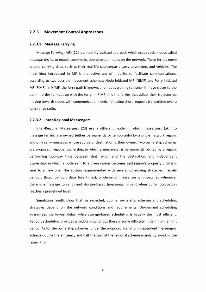
2.2.3.1 Message Ferrying

Message Ferrying (MF) [22] is a mobility-assisted approach which uses special nodes called

message ferries to enable communication between nodes on the network. These ferries move

around carrying data, such as their real-life counterparts carry passengers and vehicles. The

main idea introduced in MF is the active use of mobility to facilitate communications,

according to two possible movement schemes: Node-Initiated MF (NIMF) and Ferry-Initiated

MF (FIMF). In NIMF, the ferry path is known, and nodes waiting to transmit move closer to the

path in order to meet up with the ferry. In FIMF, it is the ferries that adjust their trajectories,

moving towards nodes with communication needs, following short requests transmitted over a

long-range radio.

2.2.3.2 Inter-Regional Messengers

Inter-Regional Messengers [23] use a different model in which messengers (akin to

message ferries) are owned (either permanently or temporarily) by a single network region,

and only carry messages whose source or destination is their owner. Two ownership schemes

are proposed: regional ownership, in which a messenger is permanently owned by a region,

performing two-way trips between that region and the destination, and independent

ownership, in which a node sent to a given region becomes said region’s property until it is

sent to a new one. The authors experimented with several scheduling strategies, namely

periodic (fixed periodic departure times), on-demand (messenger is dispatched whenever

there is a message to send) and storage-based (messenger is sent when buffer occupation

reaches a predefined level).

Simulation results show that, as expected, optimal ownership schemes and scheduling

strategies depend on the network conditions and requirements. On-demand scheduling

guarantees the lowest delay, while storage-based scheduling is usually the most efficient.

Periodic scheduling provides a middle ground, but there is some difficulty in defining the right

period. As for the ownership schemes, under the proposed scenario, independent messengers

achieve double the efficiency and half the cost of the regional scheme mainly by avoiding the

return trip.

12

2.2.3.3 Homing Pigeon based DTN

Homing Pigeon (HoP) based DTNs (HoP-DTNs) [24] are similar in model to Inter-Regional

Messengers, but are built on a theoretical framework considering message lifetimes and

simplistic assumptions. Each node has its own messenger (here called pigeon, in reference to

traditional homing pigeons), which is dispatched when s messages are buffered, and visits all

the messages’ destination nodes on a single trip, before returning to its owner. Further work

by the authors [25] introduces the concepts of regions and region-owned pigeons, also

considering the existence of multiple pigeons per region. In addition to the already discussed

on-demand and periodic scheduling strategies, the authors propose a new algorithm named

Adaptive Pigeon Scheduling (APS) which aims to increase cooperation between pigeons in the

same region and decrease average message delay.

APS is shown to consistently achieve lower delays than the other approaches, regardless

of message generation rate, pigeon speed and number, but at the cost of generally lower

energy efficiency when compared to periodic scheduling.

2.2.4 Coding-based Approaches

2.2.4.1 Erasure Coding

Erasure coding works by splitting a message into 𝑘 blocks and then expanding them to 𝑛

blocks to be transmitted in such a way that the reception of any 𝑘 of the 𝑛 is enough to

recover the original message. Several erasure coding based approaches have been proposed,

such as [26] [27] [28].

In [26] a routing approach based on erasure coding is presented. Building on the existing

2-hop routing protocol (with added message replication), the authors propose a variation in

which the sending node codes the message into 𝑘 parts, replicating it by a factor 𝑟, and

transmitting it to 𝑘𝑟 different relay nodes. The base assumption is that it is likely that 𝑘 of the

𝑘𝑟 nodes meet the destination node sooner than just 1 of the otherwise 𝑟 nodes (maintaining

the same replication factor), so delay can be reduced while maintaining the same efficiency

(the 𝑘𝑟 blocks are the same size as just the 𝑟 message copies).

Simulations were conducted using real world mobility traces from the ZebraNet project.

Results obtained under the assumption of infinite buffer space, replication factor 𝑟 = 2 and

splitting factor 𝑝 = 𝑘𝑟 = 8,16,32 show this approach to have lower delay variance than 2-

13

hop routing with the same replication factor, also beating every other tested protocol except

for pure flooding. The 50th percentile delay is generally higher than with the other approaches,

showing that very low delays are uncommon under this scheme and the majority of messages

are delivered at an almost constant, albeit moderate, delay.

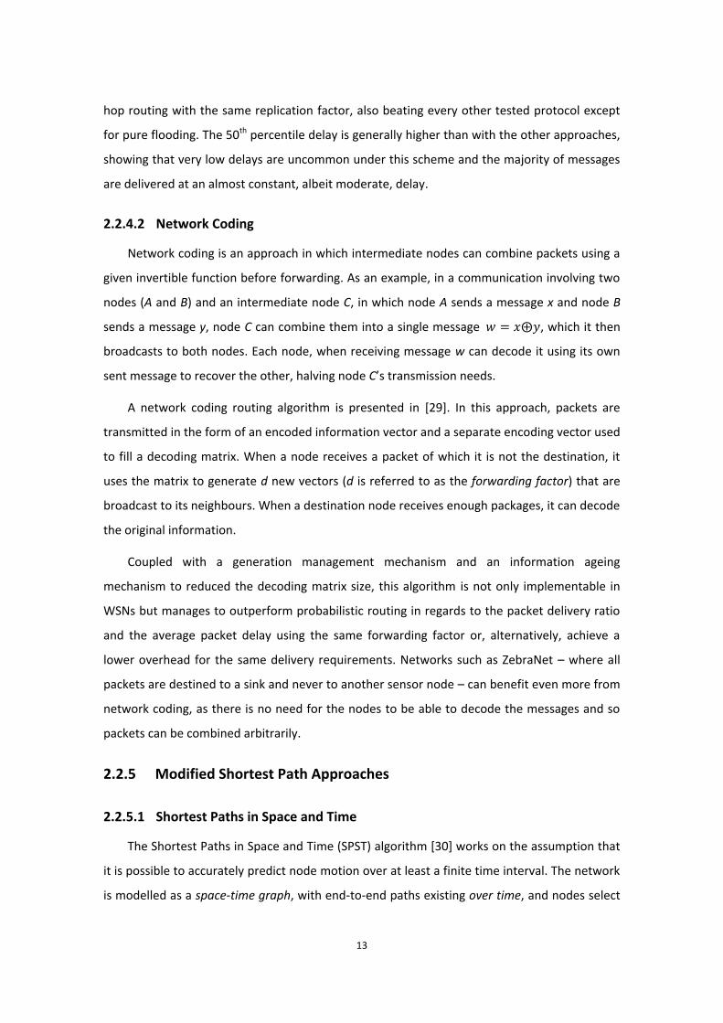
2.2.4.2 Network Coding

Network coding is an approach in which intermediate nodes can combine packets using a

given invertible function before forwarding. As an example, in a communication involving two

nodes (A and B) and an intermediate node C, in which node A sends a message x and node B

sends a message y, node C can combine them into a single message 𝑤 = 𝑥⨁𝑦, which it then

broadcasts to both nodes. Each node, when receiving message w can decode it using its own

sent message to recover the other, halving node C’s transmission needs.

A network coding routing algorithm is presented in [29]. In this approach, packets are

transmitted in the form of an encoded information vector and a separate encoding vector used

to fill a decoding matrix. When a node receives a packet of which it is not the destination, it

uses the matrix to generate d new vectors (d is referred to as the forwarding factor) that are

broadcast to its neighbours. When a destination node receives enough packages, it can decode

the original information.

Coupled with a generation management mechanism and an information ageing

mechanism to reduced the decoding matrix size, this algorithm is not only implementable in

WSNs but manages to outperform probabilistic routing in regards to the packet delivery ratio

and the average packet delay using the same forwarding factor or, alternatively, achieve a

lower overhead for the same delivery requirements. Networks such as ZebraNet – where all

packets are destined to a sink and never to another sensor node – can benefit even more from

network coding, as there is no need for the nodes to be able to decode the messages and so

packets can be combined arbitrarily.

2.2.5 Modified Shortest Path Approaches

2.2.5.1 Shortest Paths in Space and Time

The Shortest Paths in Space and Time (SPST) algorithm [30] works on the assumption that

it is possible to accurately predict node motion over at least a finite time interval. The network

is modelled as a space-time graph, with end-to-end paths existing over time, and nodes select

14

the next best hop by looking at derived space-time routing tables that include not only current

but also future neighbours. The selection algorithm, built with the aim of minimising latency, is

a Floyd-Warshall adaptation that takes into account both the destination and the message

arrival time.

Simulation results show that SPST generally behaves better than Epidemic Routing and the

other tested algorithms, providing both lower latency and higher message delivery success

ratio while achieving reduced message duplication.

2.2.5.2 Knowledge Oracles

In [31] several algorithms are proposed, all based in the concept of Knowledge Oracles,

each of the four representing some knowledge of the network at any point in time. The

Contacts Oracle contains information about node contacts; the Contacts Summary Oracle

contains aggregate statistics of these contacts; the Queuing Oracle contains information about

buffer occupation at each node; finally, the Traffic Demand Oracle contains information about

traffic demands at each node.

The used algorithm depends on which oracles are available. If all of them are, then finding

the best route is a Linear Programming (LP) problem. If at least the Contacts Summary Oracle

or the Contacts Oracle is available then a modified Dijkstra’s algorithm is used, with the cost

function depending on the specific combination of oracles.

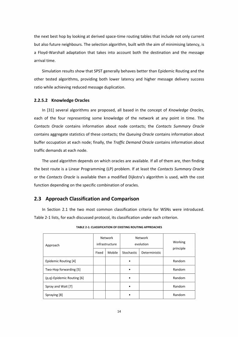
2.3 Approach Classification and Comparison

In Section 2.1 the two most common classification criteria for WSNs were introduced.

Table 2-1 lists, for each discussed protocol, its classification under each criterion.

TABLE 2-1: CLASSIFICATION OF EXISTING ROUTING APPROACHES

Approach

Network

infrastructure

Network

evolution Working

principle Fixed Mobile Stochastic Deterministic

Epidemic Routing [4] • Random

Two-Hop forwarding [5] • Random

(p,q)-Epidemic Routing [6] • Random

Spray and Wait [7] • Random

Spraying [8] • Random

15

Infostation[9] • • Random

SWIM [10] • • Random

Data MULEs [11] • • Random

ZebraNet [12] • • History

MV Routing [14] • History

PROPHET [15] • History

CAR [16] • History

SCAR [17] • History

MobySpace [18] • History

STR [19] • History

Message Ferrying [22] • • Movement control

Inter-Regional Messengers [23] • • Movement control

HoP-DTN [25] • • Movement control

Erasure Coding [26] • Coding

Network Coding [29] • Coding

SPST [30] • Shortest path

Knowledge Oracles [31] • Shortest path

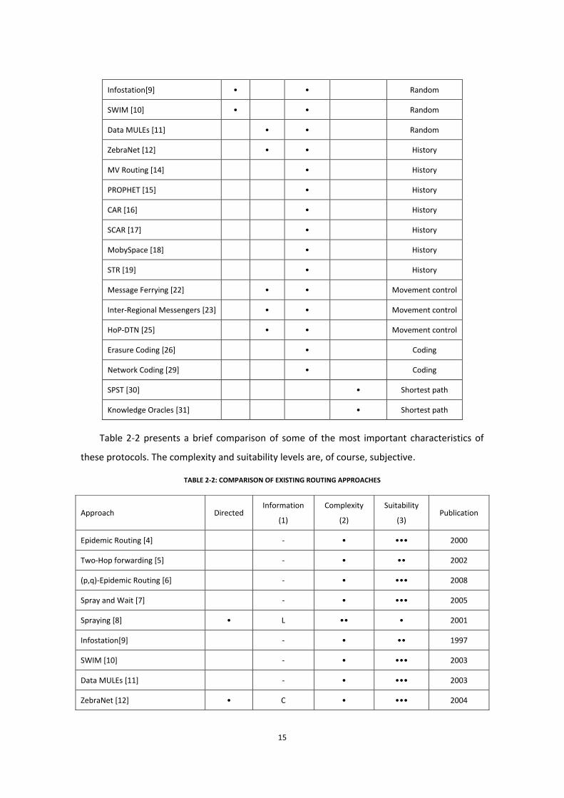
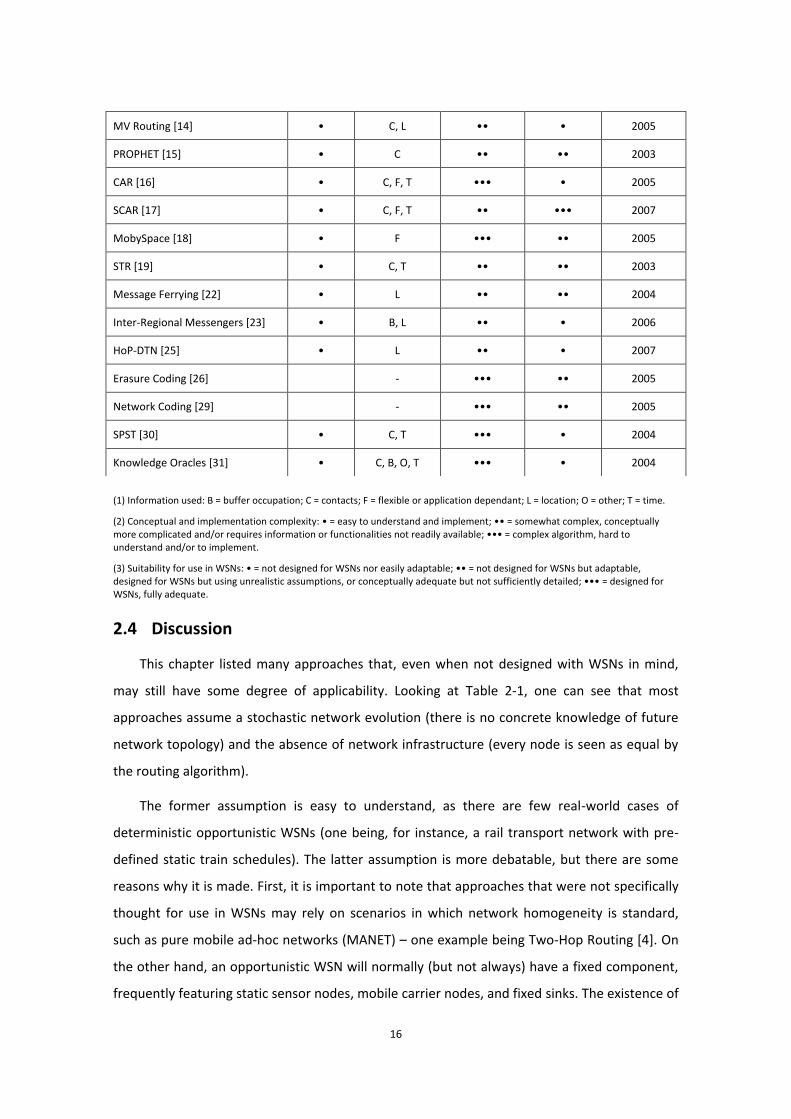
Table 2-2 presents a brief comparison of some of the most important characteristics of

these protocols. The complexity and suitability levels are, of course, subjective.

TABLE 2-2: COMPARISON OF EXISTING ROUTING APPROACHES

Approach Directed Information

(1)

Complexity

(2)

Suitability

(3) Publication

Epidemic Routing [4] - • ••• 2000

Two-Hop forwarding [5] - • •• 2002

(p,q)-Epidemic Routing [6] - • ••• 2008

Spray and Wait [7] - • ••• 2005

Spraying [8] • L •• • 2001

Infostation[9] - • •• 1997

SWIM [10] - • ••• 2003

Data MULEs [11] - • ••• 2003

ZebraNet [12] • C • ••• 2004

16

(1) Information used: B = buffer occupation; C = contacts; F = flexible or application dependant; L = location; O = other; T = time.

(2) Conceptual and implementation complexity: • = easy to understand and implement; •• = somewhat complex, conceptually more complicated and/or requires information or functionalities not readily available; ••• = complex algorithm, hard to understand and/or to implement.

(3) Suitability for use in WSNs: • = not designed for WSNs nor easily adaptable; •• = not designed for WSNs but adaptable, designed for WSNs but using unrealistic assumptions, or conceptually adequate but not sufficiently detailed; ••• = designed for WSNs, fully adequate.

2.4 Discussion

This chapter listed many approaches that, even when not designed with WSNs in mind,

may still have some degree of applicability. Looking at Table 2-1, one can see that most

approaches assume a stochastic network evolution (there is no concrete knowledge of future

network topology) and the absence of network infrastructure (every node is seen as equal by

the routing algorithm).

The former assumption is easy to understand, as there are few real-world cases of

deterministic opportunistic WSNs (one being, for instance, a rail transport network with pre-

defined static train schedules). The latter assumption is more debatable, but there are some

reasons why it is made. First, it is important to note that approaches that were not specifically

thought for use in WSNs may rely on scenarios in which network homogeneity is standard,

such as pure mobile ad-hoc networks (MANET) – one example being Two-Hop Routing [4]. On

the other hand, an opportunistic WSN will normally (but not always) have a fixed component,

frequently featuring static sensor nodes, mobile carrier nodes, and fixed sinks. The existence of

MV Routing [14] • C, L •• • 2005

PROPHET [15] • C •• •• 2003

CAR [16] • C, F, T ••• • 2005

SCAR [17] • C, F, T •• ••• 2007

MobySpace [18] • F ••• •• 2005

STR [19] • C, T •• •• 2003

Message Ferrying [22] • L •• •• 2004

Inter-Regional Messengers [23] • B, L •• • 2006

HoP-DTN [25] • L •• • 2007

Erasure Coding [26] - ••• •• 2005

Network Coding [29] - ••• •• 2005

SPST [30] • C, T ••• • 2004

Knowledge Oracles [31] • C, B, O, T ••• • 2004

17

sink nodes is assumed in most WSNs, and is not enough to classify a network as having

infrastructure. There are also fully mobile networks: ZebraNet [12], for instance, only uses

mobile sensor nodes and a mobile sink node.

Few of these approaches have withstood real world testing, and most have never even

been implemented outside the simulation environment used by the authors. The most used

are probably the Epidemic Routing algorithm [4] and the ZebraNet history-based algorithm

[12], which are also two of the simplest. This should come as no surprise given that, by

increasing routing complexity and/or expanding the underlying assumptions, many algorithms

are implicitly restricting their applicability, either because of hardware limitations, lack of

required information or plain inadequacy to the network structure, requirements or

movement patterns. Some algorithms do this in accordance with the longstanding trend in

WSNs (or, to be precise, in any heavily constrained system) of using scenario-specific solutions

as a way to optimize performance. Others go the opposite direction, aiming for such generality

that they become too complex for any real scenario.

18

3 Target Scenario and Network Architecture

There are uncountable different WSN usage scenarios. As previously stated, it is very hard,

if not impossible, to develop a true general-purpose solution. To be realistic, a sensible set of

restrictions must be specified. Architectural aspects of the network are tightly coupled to these

restrictions, hence they are jointly described.

Sparse networks, those with low node density, are the most challenging from an OR point

of view, since decisions carry a graver impact on global performance. They are also the ones

most in need of OR solutions, as high-density networks can in most cases make use of other

approaches, namely traditional ad-hoc routing. Networks are also assumed to be highly

scattered, with permanently-connected partitions being a rare occurrence. This negates the

need for hybrid routing protocols, which include a separate, non-opportunistic mechanism for

routing inside these partitions.

Highly mobile networks, in which the majority of nodes (or, in the limiting case, all of

them) move, also make for a more interesting case, as mostly static networks are easily served

by a MULE-like architecture [11]. Passive mobility is another reasonable assumption. Even

though there are cases in which it makes sense to have on-demand mobile agents, these

constitute a minority due to cost and complexity. Networks with deterministic evolution are

seldom found and well served by existing solutions, so it makes sense to focus on those with

stochastic evolution. That does not imply, however, the total absence of movement patterns

on the network: if that were the case, no routing algorithm would do better than a random

forwarding approach. Consequences of high-speed movement, found in scenarios such as

motorways and railway networks, are outside the scope of this work.

For realism’s sake, resource constraints must also be taken into account. While sensor

nodes are becoming more powerful each day, they will keep on being a heavily-constrained

system in the foreseeable future. Radio range and bitrate, processor speed, memory capacity

and energy are examples of scarce resources. Energy limitations are perhaps the most serious:

the reduced size and cost of nodes prevent the use of long-life batteries, and while there are

energy-harvesting solutions, these too are expensive, inefficient or impractical.

Finally, in most sensor networks, the goal is to collect data from sensors and deliver it to a

central node (sink) for analysis. This is best accomplished by using what is commonly known as

19

a single-tree convergecast architecture. Additionally, an any-sink property is assumed,

meaning that several sinks may exist, and delivery to any one of them is sufficient.

In short, the focus has been placed on low-density, highly mobile networks with stochastic

evolution and convergecast architecture, possibly using multiple sinks. Nodes are assumed to

be resource-constrained, particularly in relation to energy. This is a reasonable set of

assumptions and the resulting scenario is commonly found in real-world applications including

environmental, wildlife and silvopastoral systems monitoring.

3.1 Example scenario – Organic Silvopastoral Systems

Organic farming is assuming an increasing importance all over Europe due to its perceived

higher product quality, possible health benefits and reduced environmental impact. It is based

on the use of natural processes and subject to hard, government regulated constraints on the

use of chemical helpers such as synthetic fertilisers and pesticides. Animals grown under

organic farming regimes are also subject to the same constraints, and must generally be fed

with natural products, these too coming from organic farms.

These requirements create an incentive for the use of a holistic model, taking advantage

of synergies between both practices: free-grazing livestock (most commonly sheep, goats,

cattle, pigs and horses) provide fertilization, control the proliferation of invasive plants and

reduce fire hazard, while at the same time naturally feeding and using the trees for shelter.

Traditional silvopastoral systems are abundant all over the world. In the Portuguese case,

the main ones are plantations of Cork Oak (the montado), Pyrenean Oak, Chestnut and Olive

Tree orchards, with the last maybe being “the most complete multipurpose form of land use in

the world” [32]. While the industrial high-yield agriculture trends of the last decades have

threatened these systems, the new trend towards organic farming (and the high economic

value of organic olive oil) is thought to open the gates for its survival and expansion.

There is presently interest in using WSNs for monitoring several cultures, seeing as they

present undeniable advantages, but most proposed systems assume some form of long-range

communication, typically public cellular networks. Even though there is also some research on

livestock monitoring WSNs, no project combines both.

The use of an opportunistic WSN integrating both tree-mounted sensor nodes and

livestock carried sensor nodes would allow monitoring of the whole system, and using the

animals as information carriers would drop the dependency on external communication

20

systems and its associated costs. Several solar-powered sinks could be deployed on sites the

animals are known to frequently visit, and relay data via a long-range radio link.

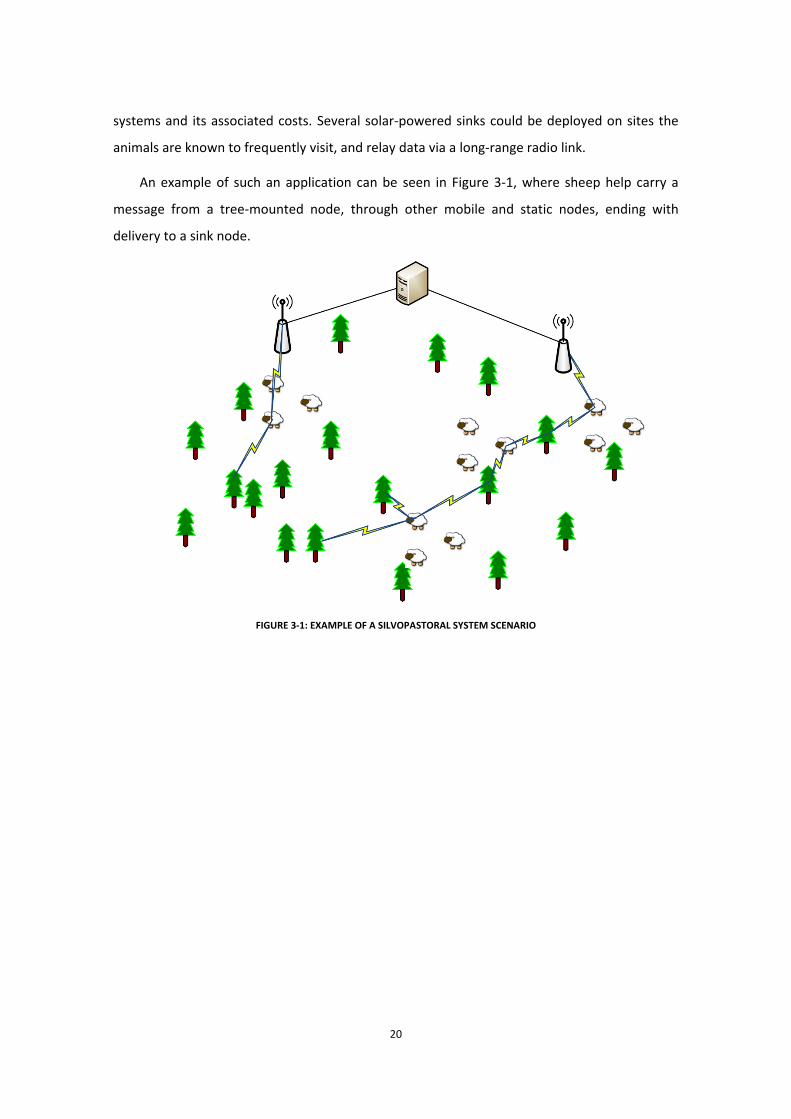
An example of such an application can be seen in Figure 3-1, where sheep help carry a

message from a tree-mounted node, through other mobile and static nodes, ending with

delivery to a sink node.

FIGURE 3-1: EXAMPLE OF A SILVOPASTORAL SYSTEM SCENARIO

21

4 CHARON Design

In this chapter the main considerations behind CHARON’s design will be discussed. The

initial design goals will be listed, followed by a brief overview of the approach, a detailed

description of the mechanisms used, and the reasons leading to their selection.

4.1 Design Goals

Considering the target scenario, four main goals were defined for the development of

CHARON: reliability, simplicity, efficiency and flexibility. Some of these goals are in conflict with

each other, e.g., increasing reliability may require a less efficient solution. In the course of the

design phase, choices had to be made to achieve a balanced solution.

Reliability. This is the basic goal of any routing solution, and the single goal of many. It can

be defined as the delivery the largest possible fraction of messages, in a limited time frame,

while they are still useful for the application. Note that, beyond guaranteeing a message

arrives within its usefulness window, minimizing delivery delay isn’t necessarily a concern.

Simplicity. Simplicity in this context comprises not only computational simplicity, but also

that of the implementation. Computational simplicity is necessary because the available

hardware has severe resource constraints. Even if resources suffice to run somewhat complex

routing protocols, the network’s objective is not to route messages but to run an application,

and the bulk of resources should be left for the application to use. A solution is of limited

usefulness if it is hard to implement or deploy, and so the developed solution should be easily

implemented in any platform. For the same reason, dependencies on hardware that is not

normally available must also be avoided.

Efficiency. The least possible amount of resources should be required to execute the

required tasks. That includes using less memory, transmitting fewer messages and spending

less energy. By minimizing the number of transmissions, memory requirements are usually

reduced, and in some cases energy can also be saved2. Energy-efficiency does nonetheless

require additional thought, and frequently involves specific power management mechanisms.

Flexibility. The developed solution should be usable in many settings, provided these

settings fit the target scenario. To accomplish this goal, design has to be done with (relative)

2 Some radios use more energy while idle listening than while transmitting. In those radios, reducing the number of transmissions has no direct impact on energy usage. Nevertheless, by transmitting less messages, the radio rests unused for longer periods, and can be turned off.

22

generality in mind, right from the start. Nevertheless, all applications have specificities, and

the system must be easy to customize to each specific setting. Finally, there is the question of

intra-scenario flexibility: even in the same network there may be different requirements for

different data. The solution should be able to accommodate all these requirements.

4.2 Solution Overview

CHARON is a history-based routing algorithm. It shares the same basic operating principle

as other algorithms in that class: nodes exchange and/or record some kind of historic

information when they meet, and make routing decisions based on that information. The main

historic routing metric used in CHARON is delay, as previously proposed in other contexts [33].

The expected delivery delay through each node (its Estimated Delivery Delay or EDD) is

determined, and messages are routed along a decreasing delay gradient having a sink node as

its end. The decision to use this metric, versus, for instance, the nodes’ relative mobility or sink

encounter frequency, was made in an effort to align the mechanism to the goal, which is to get

the data to the sinks before it expires (see Section 4.3).

Nonetheless, optimizing delay isn’t the only concern, as limited network resources should

also be considered in order to provide a truly efficient solution. To accommodate that

requirement, while also providing easy customizability, a multivariate utility function is used to

compute an additional score for each node. The utility function is of optional character: if

undefined, routing is based solely on minimizing the delay. If it is defined, it can use the

CHARON-provided free buffer space and available energy data, and/or draw on other

application- or system-provided metrics (see Section 4.3.2).

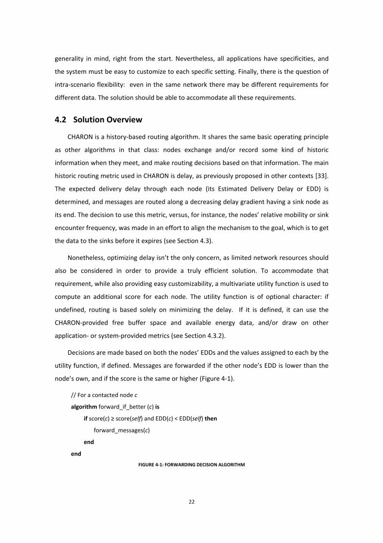
Decisions are made based on both the nodes’ EDDs and the values assigned to each by the

utility function, if defined. Messages are forwarded if the other node’s EDD is lower than the

node’s own, and if the score is the same or higher (Figure 4-1).

// For a contacted node c

algorithm forward_if_better (c) is

if score(c) ≥ score(self) and EDD(c) < EDD(self) then

forward_messages(c)

end

end

FIGURE 4-1: FORWARDING DECISION ALGORITHM

23

Messages are basically forwarded using a single-copy approach, meaning that there is but

one copy of a message in the network at any single time. Nonetheless, there is always implicit

message copying, as every time a message is forwarded a copy is left behind. Instead of

deleting messages on transmission, CHARON retains them in a special state that doesn’t allow

forwarding except in the case that the node meets a sink. Messages in this state are known as

zombies, and the strategy was named hybrid replication. The traditional multi-copy paradigm is

also supported for situations that require it (see Section 4.3.3).

In order to realize the intra-scenario flexibility objective, basic Quality of Service (QoS)

mechanisms were designed into the solution. QoS classes may be configured, and each can use

a different replication strategy and utility function. This allows CHARON to provide very

reliable (though inefficient) service to urgent or important messages, whilst maintaining high

efficiency for the majority of (delay and disruption tolerant) messages (see Section 4.3.4).

As minimizing the number of transmissions isn’t enough to provide an energy-efficient

solution, CHARON has built-in support for synchronous radio power management, significantly

reducing energy waste (see Section 4.3.5). As a global time reference is not always available, a

very simple and low-precision synchronization mechanism was integrated, making use of just

two values: the reference and the reference age (see Section 4.3.6).

CHARON operates as a bundle layer, being implemented on top of the network stack

provided with the platform. By relying on already available lower-level protocols and avoiding

duplicated functionality, this approach manages to significantly reduce the size and complexity

of CHARON’s implementation. There is a small impact on communication efficiency, leading to

longer frames due to extra encapsulation – a generally advantageous trade-off. Furthermore, it

helps make the solution platform-agnostic and independent of the low-level details. There are

only two types of messages in CHARON: beacons, which relay routing information, and

bundles, which carry application data. Through the entire document, the terms message and

bundle are used interchangeably, unless otherwise noted (see Section 4.4).

24

4.3 Feature Design

4.3.1 Delay-Based Routing

The main goal is to route messages in such a way that their expected delivery delay

decreases with each hop. To do so, the expected delivery delay of each node must be

estimated, considering its movement patterns. Two parameters are defined:

Estimated Delivery Delay (EDD) is a characteristic of each node, and describes the

estimated time a message delivered to that node will take to reach a sink. Sink

nodes have an EDD of 0.

Inter-Contact Time (ICT) is a characteristic of each node pair (or link), and is a

measure of the expected time between encounters of those two nodes. The ICT is

not defined (or can be thought of as infinite) for a pair of nodes that never met.

A node (𝑣 ∈ 𝑉) maintains a list of its contacts (𝑉𝑣 ⊆ 𝑉) and records the advertised EDD for

each contacted node. It also computes the ICT, through an exponentially weighted moving

average (EWMA) of the intervals between previous encounters. From node 𝑣’s perspective,

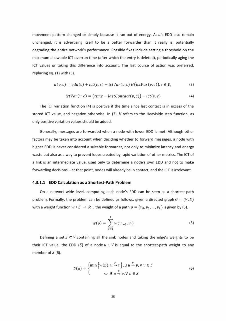
the perceived delay (𝑑) through a known contact (𝑐) is given by the sum of its EDD (𝑒𝑑𝑑 ∶ 𝑉𝑐 →

ℛ+) and the ICT (𝑖𝑐𝑡 ∶ 𝑉, 𝑉𝑣 → ℛ+) between both nodes (1).

𝑑 𝑣, 𝑐 = 𝑒𝑑𝑑 𝑐 + 𝑖𝑐𝑡 𝑣, 𝑐 , 𝑐 ∈ 𝑉𝑣 (1)

In fact, ICT describes the expected worst case encounter delay so, for the average delay,

its half should be considered. Yet both strategies are equivalent as long as there is coherence,

and this way the number of required arithmetic operations is reduced.

A node’s EDD is equal to the minimum achievable delay, or the delay through the quickest

known node, given by (2).

𝑒𝑑𝑑 𝑣 = min𝑐 ∈ 𝑉𝑣

{𝑑(𝑣, 𝑐)} (2)

In practice, this means CHARON uses a transitive delay metric with an additive

concatenation operator and an extra variable per-hop factor. As a consequence, EDD is only

defined for nodes with a complete chain of contacts ending in a sink.

A problem with this approach is that ICTs don’t degrade naturally, that is, if two nodes

(𝑎, 𝑏, ⊂ 𝑉) don’t meet, their ICT value stays unchanged. This may have serious consequences if

𝑏 is 𝑎’s best known forwarder, and 𝑏 stops being a good forwarder, perhaps because its

25

movement pattern changed or simply because it ran out of energy. As 𝑎’s EDD also remain

unchanged, it is advertising itself to be a better forwarder than it really is, potentially

degrading the entire network’s performance. Possible fixes include setting a threshold on the

maximum allowable ICT overrun time (after which the entry is deleted), periodically aging the

ICT values or taking this difference into account. The last course of action was preferred,

replacing eq. (1) with (3).

𝑑 𝑣, 𝑐 = 𝑒𝑑𝑑 𝑐 + 𝑖𝑐𝑡 𝑣, 𝑐 + 𝑖𝑐𝑡𝑉𝑎𝑟 𝑣, 𝑐 𝐻 𝑖𝑐𝑡𝑉𝑎𝑟 𝑣, 𝑐 , 𝑐 ∈ 𝑉𝑣 (3)

𝑖𝑐𝑡𝑉𝑎𝑟 𝑣, 𝑐 = 𝑡𝑖𝑚𝑒 − 𝑙𝑎𝑠𝑡𝐶𝑜𝑛𝑡𝑎𝑐𝑡 𝑣, 𝑐 − 𝑖𝑐𝑡(𝑣, 𝑐) (4)

The ICT variation function (4) is positive if the time since last contact is in excess of the

stored ICT value, and negative otherwise. In (3), 𝐻 refers to the Heaviside step function, as

only positive variation values should be added.

Generally, messages are forwarded when a node with lower EDD is met. Although other

factors may be taken into account when deciding whether to forward messages, a node with

higher EDD is never considered a suitable forwarder, not only to minimize latency and energy

waste but also as a way to prevent loops created by rapid variation of other metrics. The ICT of

a link is an intermediate value, used only to determine a node’s own EDD and not to make

forwarding decisions – at that point, nodes will already be in contact, and the ICT is irrelevant.

4.3.1.1 EDD Calculation as a Shortest-Path Problem

On a network-wide level, computing each node’s EDD can be seen as a shortest-path

problem. Formally, the problem can be defined as follows: given a directed graph 𝐺 = (𝑉, 𝐸)

with a weight function 𝑤 ∶ 𝐸 → ℛ+, the weight of a path 𝑝 = {𝑣0 , 𝑣1 , … , 𝑣𝑘} is given by (5).

𝑤 𝑝 = 𝑤(𝑣𝑖−1 , 𝑣𝑖)

𝑘

𝑖=1

(5)

Defining a set 𝑆 ⊂ 𝑉 containing all the sink nodes and taking the edge’s weights to be

their ICT value, the EDD (𝛿) of a node 𝑢 ∈ 𝑉 is equal to the shortest-path weight to any

member of 𝑆 (6).

𝛿 𝑢 = min 𝑤 𝑝 : 𝑢

𝑝→ 𝑣 , ∃ 𝑢

𝑝→ 𝑣, ∀ 𝑣 ∈ 𝑆

∞ , ∄ 𝑢𝑝→ 𝑣, ∀ 𝑣 ∈ 𝑆

(6)

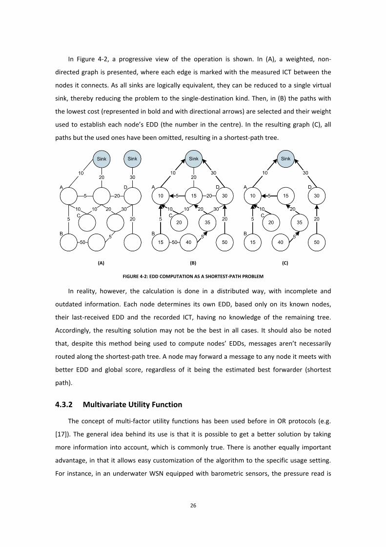
26

In Figure 4-2, a progressive view of the operation is shown. In (A), a weighted, non-

directed graph is presented, where each edge is marked with the measured ICT between the

nodes it connects. As all sinks are logically equivalent, they can be reduced to a single virtual

sink, thereby reducing the problem to the single-destination kind. Then, in (B) the paths with

the lowest cost (represented in bold and with directional arrows) are selected and their weight

used to establish each node’s EDD (the number in the centre). In the resulting graph (C), all

paths but the used ones have been omitted, resulting in a shortest-path tree.

(A)

(B)

(C)

FIGURE 4-2: EDD COMPUTATION AS A SHORTEST-PATH PROBLEM

In reality, however, the calculation is done in a distributed way, with incomplete and

outdated information. Each node determines its own EDD, based only on its known nodes,

their last-received EDD and the recorded ICT, having no knowledge of the remaining tree.

Accordingly, the resulting solution may not be the best in all cases. It should also be noted

that, despite this method being used to compute nodes’ EDDs, messages aren’t necessarily

routed along the shortest-path tree. A node may forward a message to any node it meets with

better EDD and global score, regardless of it being the estimated best forwarder (shortest

path).

4.3.2 Multivariate Utility Function

The concept of multi-factor utility functions has been used before in OR protocols (e.g.

[17]). The general idea behind its use is that it is possible to get a better solution by taking

more information into account, which is commonly true. There is another equally important

advantage, in that it allows easy customization of the algorithm to the specific usage setting.

For instance, in an underwater WSN equipped with barometric sensors, the pressure read is

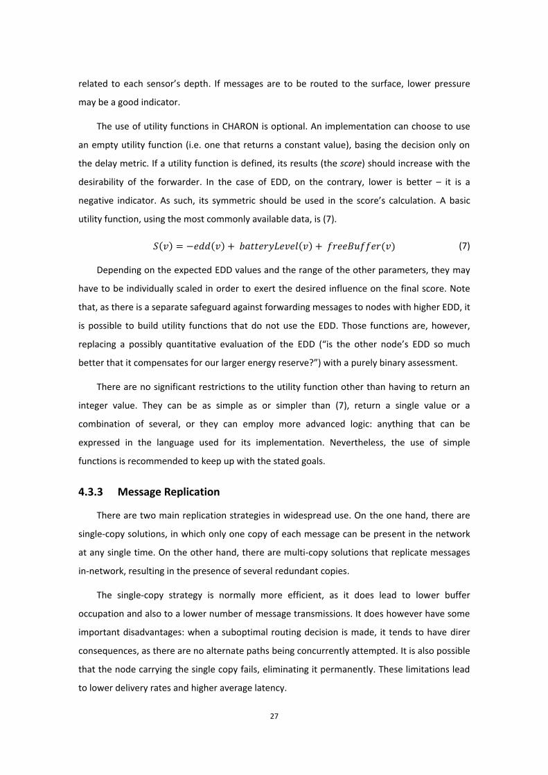
27

related to each sensor’s depth. If messages are to be routed to the surface, lower pressure

may be a good indicator.

The use of utility functions in CHARON is optional. An implementation can choose to use

an empty utility function (i.e. one that returns a constant value), basing the decision only on

the delay metric. If a utility function is defined, its results (the score) should increase with the

desirability of the forwarder. In the case of EDD, on the contrary, lower is better – it is a

negative indicator. As such, its symmetric should be used in the score’s calculation. A basic

utility function, using the most commonly available data, is (7).

𝑆 𝑣 = −𝑒𝑑𝑑 𝑣 + 𝑏𝑎𝑡𝑡𝑒𝑟𝑦𝐿𝑒𝑣𝑒𝑙 𝑣 + 𝑓𝑟𝑒𝑒𝐵𝑢𝑓𝑓𝑒𝑟(𝑣) (7)

Depending on the expected EDD values and the range of the other parameters, they may

have to be individually scaled in order to exert the desired influence on the final score. Note

that, as there is a separate safeguard against forwarding messages to nodes with higher EDD, it

is possible to build utility functions that do not use the EDD. Those functions are, however,

replacing a possibly quantitative evaluation of the EDD (“is the other node’s EDD so much

better that it compensates for our larger energy reserve?”) with a purely binary assessment.

There are no significant restrictions to the utility function other than having to return an

integer value. They can be as simple as or simpler than (7), return a single value or a

combination of several, or they can employ more advanced logic: anything that can be

expressed in the language used for its implementation. Nevertheless, the use of simple

functions is recommended to keep up with the stated goals.

4.3.3 Message Replication

There are two main replication strategies in widespread use. On the one hand, there are

single-copy solutions, in which only one copy of each message can be present in the network

at any single time. On the other hand, there are multi-copy solutions that replicate messages

in-network, resulting in the presence of several redundant copies.

The single-copy strategy is normally more efficient, as it does lead to lower buffer

occupation and also to a lower number of message transmissions. It does however have some

important disadvantages: when a suboptimal routing decision is made, it tends to have direr

consequences, as there are no alternate paths being concurrently attempted. It is also possible

that the node carrying the single copy fails, eliminating it permanently. These limitations lead

to lower delivery rates and higher average latency.

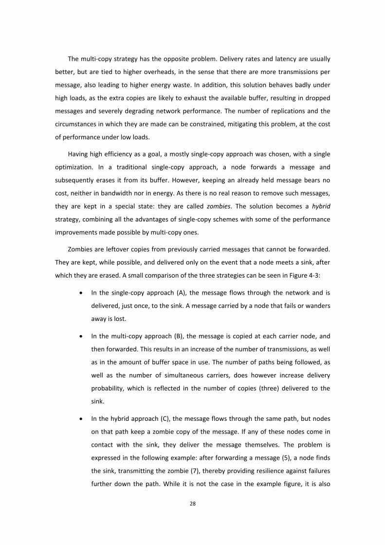
28

The multi-copy strategy has the opposite problem. Delivery rates and latency are usually

better, but are tied to higher overheads, in the sense that there are more transmissions per

message, also leading to higher energy waste. In addition, this solution behaves badly under

high loads, as the extra copies are likely to exhaust the available buffer, resulting in dropped

messages and severely degrading network performance. The number of replications and the

circumstances in which they are made can be constrained, mitigating this problem, at the cost

of performance under low loads.

Having high efficiency as a goal, a mostly single-copy approach was chosen, with a single

optimization. In a traditional single-copy approach, a node forwards a message and

subsequently erases it from its buffer. However, keeping an already held message bears no

cost, neither in bandwidth nor in energy. As there is no real reason to remove such messages,

they are kept in a special state: they are called zombies. The solution becomes a hybrid

strategy, combining all the advantages of single-copy schemes with some of the performance

improvements made possible by multi-copy ones.

Zombies are leftover copies from previously carried messages that cannot be forwarded.

They are kept, while possible, and delivered only on the event that a node meets a sink, after

which they are erased. A small comparison of the three strategies can be seen in Figure 4-3:

In the single-copy approach (A), the message flows through the network and is

delivered, just once, to the sink. A message carried by a node that fails or wanders

away is lost.

In the multi-copy approach (B), the message is copied at each carrier node, and

then forwarded. This results in an increase of the number of transmissions, as well

as in the amount of buffer space in use. The number of paths being followed, as

well as the number of simultaneous carriers, does however increase delivery

probability, which is reflected in the number of copies (three) delivered to the

sink.

In the hybrid approach (C), the message flows through the same path, but nodes

on that path keep a zombie copy of the message. If any of these nodes come in

contact with the sink, they deliver the message themselves. The problem is

expressed in the following example: after forwarding a message (5), a node finds

the sink, transmitting the zombie (7), thereby providing resilience against failures

further down the path. While it is not the case in the example figure, it is also

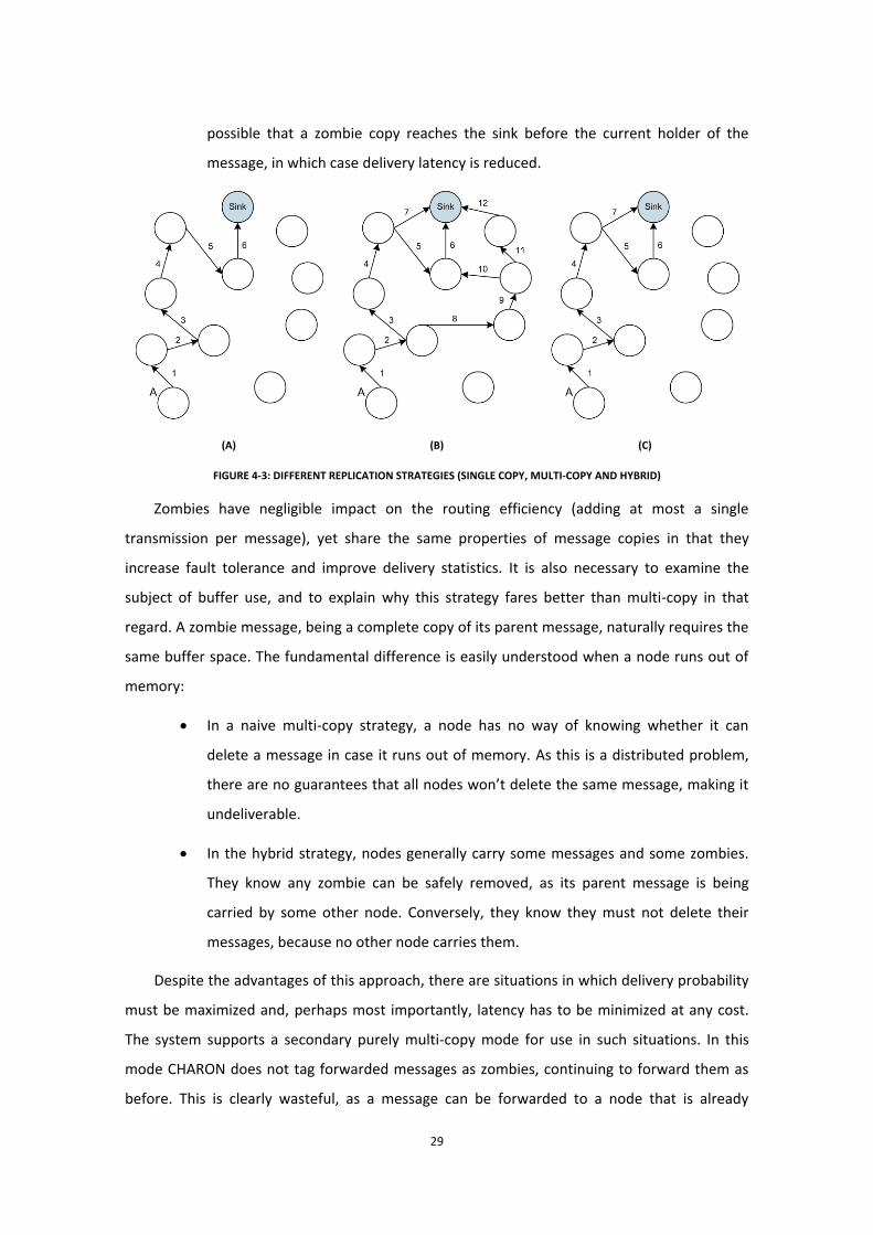
29

possible that a zombie copy reaches the sink before the current holder of the

message, in which case delivery latency is reduced.

(A)

(B)

(C)

FIGURE 4-3: DIFFERENT REPLICATION STRATEGIES (SINGLE COPY, MULTI-COPY AND HYBRID)

Zombies have negligible impact on the routing efficiency (adding at most a single

transmission per message), yet share the same properties of message copies in that they

increase fault tolerance and improve delivery statistics. It is also necessary to examine the

subject of buffer use, and to explain why this strategy fares better than multi-copy in that

regard. A zombie message, being a complete copy of its parent message, naturally requires the

same buffer space. The fundamental difference is easily understood when a node runs out of

memory:

In a naive multi-copy strategy, a node has no way of knowing whether it can

delete a message in case it runs out of memory. As this is a distributed problem,

there are no guarantees that all nodes won’t delete the same message, making it

undeliverable.

In the hybrid strategy, nodes generally carry some messages and some zombies.

They know any zombie can be safely removed, as its parent message is being

carried by some other node. Conversely, they know they must not delete their

messages, because no other node carries them.

Despite the advantages of this approach, there are situations in which delivery probability

must be maximized and, perhaps most importantly, latency has to be minimized at any cost.

The system supports a secondary purely multi-copy mode for use in such situations. In this

mode CHARON does not tag forwarded messages as zombies, continuing to forward them as

before. This is clearly wasteful, as a message can be forwarded to a node that is already

30

carrying it, but unavoidable without introducing additional message types or additional beacon

fields. Given that this mode is meant to be seldom used, the introduction of additional

complex mechanisms has been avoided. A node can however keep track of other nodes to

which it has already forwarded each message and refrain from forwarding to them again.

While this mode does succeed in improving delivery statistics, it has a negative impact on the

network as a whole if abused, and should only be employed when strictly required.

4.3.4 Quality of Service

Even within specific applications, there are sometimes messages with different

requirements. A simple example is that of an agricultural monitoring WSN: while most

messages probably contain only temperature, humidity and PH samples and are not urgent,

there can also be alarm messages alerting the operators to a pest or a fire threatening

production and requiring immediate attention. This coexistence of different requirements

within the same network is the motivation for including quality-of-service (QoS) mechanisms in

CHARON.

Before going into details, it is important to clarify that the definition of QoS in this context

is limited to the ability to provide different performance levels to different data classes.

Resource reservation and service level guarantees are difficult (if not impossible) to put into

practice in the target scenario and within the stated goals, and as such weren’t considered. In

that sense, the service CHARON provides is always best-effort.

The customizability of some parts of CHARON was previously discussed, in what refers to

the particularities of the deployment scenario. The system is even more adaptable as it can be

customized for individual traffic classes within the same deployment. There are three

independently configurable class-specific features:

Utility function

Replication strategy

Time to Live (TTL) value

Depending on the chosen settings, the result can range from purely delay-based, multi-

copy routing with high overhead but low latency, to very efficient, single-copy, energy-aware

routing. While CHARON supports an unlimited number of classes, in the vast majority of cases

two will be sufficient:

31

A low-priority class used for bulk monitoring data, configured with an energy-

aware utility function and hybrid replication

A high-priority class used for urgent alarm data, configured with no utility function

and multi-copy replication

An example of such an arrangement is presented in Table 4-1, where different TTL values

were also defined. The choice of TTL parameters should take into account the period during

which data is useful. Alarm data is, by definition, urgent and – considering the wasteful

mechanism being used to route it – should be set to expire as soon as possible.

TABLE 4-1: EXAMPLE CLASS CONFIGURATION

Class Utility function Replication strategy TTL value

Monitoring 𝑆 𝑐 = −𝑒𝑑𝑑 𝑐 + 𝑓𝑟𝑒𝑒𝐵𝑢𝑓𝑓𝑒𝑟 𝑐 + 𝑏𝑎𝑡𝑡𝑒𝑟𝑦𝐿𝑒𝑣𝑒𝑙(𝑐) Hybrid 72 h

Alarm 𝑆(𝑐) = 0 Multi-copy 12 h

Using this simple scheme, CHARON is able to provide multi-copy-like performance on

high-priority messages, as long as they are few and far in between, while still keeping global

overhead at very low levels. It must be emphasised that this is only true if alarm messages

account for a small fraction of the total as otherwise global performance will be severely

degraded.

4.3.5 Power Management

Regardless of how high an algorithm’s routing efficiency is, it can’t achieve good energy

efficiency per se. Broadband radios are not only one of the largest consumers but can use as

much or even more energy on idle listening than they do while transmitting. To save energy,

this must be taken into account by turning off the radio when it is not necessary.

There are several possible radio power management approaches including synchronous

[34] and asynchronous [35] [36] cycling, as well as more advanced, on-demand solutions such

as wake-up radios [37]. Asynchronous cycling presents a sub-optimal solution, requiring very

short rounds that may inhibit advanced power saving modes, and can lead to long always-on

periods if trying to transmit in the absence of neighbours. The use of wake-up radios seems

promising but requires additional hardware on most current platforms. This leaves

synchronous cycling, which is generally a good solution although it requires a global time

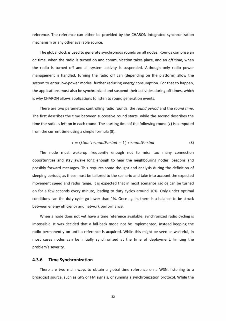
32

reference. The reference can either be provided by the CHARON-integrated synchronization

mechanism or any other available source.

The global clock is used to generate synchronous rounds on all nodes. Rounds comprise an

on time, when the radio is turned on and communication takes place, and an off time, when

the radio is turned off and all system activity is suspended. Although only radio power

management is handled, turning the radio off can (depending on the platform) allow the

system to enter low-power modes, further reducing energy consumption. For that to happen,

the applications must also be synchronized and suspend their activities during off times, which

is why CHARON allows applications to listen to round generation events.

There are two parameters controlling radio rounds: the round period and the round time.

The first describes the time between successive round starts, while the second describes the

time the radio is left on in each round. The starting time of the following round (𝜏) is computed

from the current time using a simple formula (8).

𝜏 = 𝑡𝑖𝑚𝑒 \ 𝑟𝑜𝑢𝑛𝑑𝑃𝑒𝑟𝑖𝑜𝑑 + 1 ∗ 𝑟𝑜𝑢𝑛𝑑𝑃𝑒𝑟𝑖𝑜𝑑 (8)

The node must wake-up frequently enough not to miss too many connection

opportunities and stay awake long enough to hear the neighbouring nodes’ beacons and

possibly forward messages. This requires some thought and analysis during the definition of

sleeping periods, as these must be tailored to the scenario and take into account the expected

movement speed and radio range. It is expected that in most scenarios radios can be turned

on for a few seconds every minute, leading to duty cycles around 10%. Only under optimal

conditions can the duty cycle go lower than 1%. Once again, there is a balance to be struck

between energy efficiency and network performance.

When a node does not yet have a time reference available, synchronized radio cycling is

impossible. It was decided that a fall-back mode not be implemented, instead keeping the

radio permanently on until a reference is acquired. While this might be seen as wasteful, in

most cases nodes can be initially synchronized at the time of deployment, limiting the

problem’s severity.

4.3.6 Time Synchronization

There are two main ways to obtain a global time reference on a WSN: listening to a

broadcast source, such as GPS or FM signals, or running a synchronization protocol. While the

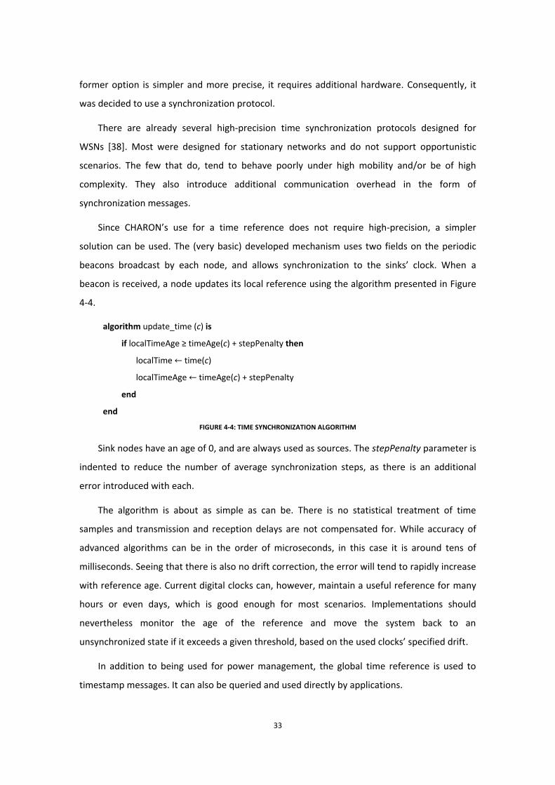
33

former option is simpler and more precise, it requires additional hardware. Consequently, it

was decided to use a synchronization protocol.

There are already several high-precision time synchronization protocols designed for

WSNs [38]. Most were designed for stationary networks and do not support opportunistic

scenarios. The few that do, tend to behave poorly under high mobility and/or be of high

complexity. They also introduce additional communication overhead in the form of

synchronization messages.

Since CHARON’s use for a time reference does not require high-precision, a simpler

solution can be used. The (very basic) developed mechanism uses two fields on the periodic

beacons broadcast by each node, and allows synchronization to the sinks’ clock. When a

beacon is received, a node updates its local reference using the algorithm presented in Figure

4-4.

algorithm update_time (c) is

if localTimeAge ≥ timeAge(c) + stepPenalty then

localTime ← time(c)

localTimeAge ← timeAge(c) + stepPenalty

end

end

FIGURE 4-4: TIME SYNCHRONIZATION ALGORITHM

Sink nodes have an age of 0, and are always used as sources. The stepPenalty parameter is

indented to reduce the number of average synchronization steps, as there is an additional

error introduced with each.

The algorithm is about as simple as can be. There is no statistical treatment of time

samples and transmission and reception delays are not compensated for. While accuracy of

advanced algorithms can be in the order of microseconds, in this case it is around tens of

milliseconds. Seeing that there is also no drift correction, the error will tend to rapidly increase

with reference age. Current digital clocks can, however, maintain a useful reference for many

hours or even days, which is good enough for most scenarios. Implementations should

nevertheless monitor the age of the reference and move the system back to an

unsynchronized state if it exceeds a given threshold, based on the used clocks’ specified drift.

In addition to being used for power management, the global time reference is used to

timestamp messages. It can also be queried and used directly by applications.

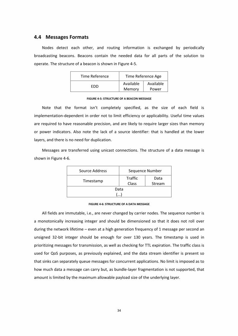
34

4.4 Messages Formats

Nodes detect each other, and routing information is exchanged by periodically

broadcasting beacons. Beacons contain the needed data for all parts of the solution to

operate. The structure of a beacon is shown in Figure 4-5.

Time Reference Time Reference Age

EDD Available Memory

Available Power

FIGURE 4-5: STRUCTURE OF A BEACON MESSAGE

Note that the format isn’t completely specified, as the size of each field is

implementation-dependent in order not to limit efficiency or applicability. Useful time values

are required to have reasonable precision, and are likely to require larger sizes than memory

or power indicators. Also note the lack of a source identifier: that is handled at the lower

layers, and there is no need for duplication.

Messages are transferred using unicast connections. The structure of a data message is

shown in Figure 4-6.

Source Address Sequence Number

Timestamp Traffic Class

Data Stream

Data (...)

FIGURE 4-6: STRUCTURE OF A DATA MESSAGE

All fields are immutable, i.e., are never changed by carrier nodes. The sequence number is

a monotonically increasing integer and should be dimensioned so that it does not roll over

during the network lifetime – even at a high generation frequency of 1 message per second an

unsigned 32-bit integer should be enough for over 130 years. The timestamp is used in

prioritizing messages for transmission, as well as checking for TTL expiration. The traffic class is

used for QoS purposes, as previously explained, and the data stream identifier is present so

that sinks can separately queue messages for concurrent applications. No limit is imposed as to

how much data a message can carry but, as bundle-layer fragmentation is not supported, that

amount is limited by the maximum allowable payload size of the underlying layer.

35

There are no other routing-specific messages, in an effort to maintain the approach’s

simplicity. This also means there are no bundle-layer acknowledgements; it is a non-

conversational protocol. Data loss is prevented by relying on lower-layer acknowledgements.

36

5 Reference Implementation

A reference implementation of CHARON was developed, primarily as a proof of concept. It

is meant to allow validation and evaluation of the proposed solution in a real setting. It also

helped to better assess the difficulty of implementing CHARON in real WSN hardware. This

chapter describes the implementation’s architecture.

5.1 Development Platform

Most previous [39] [34] and ongoing WSN experiments at GEMS3 have used Crossbow

MICAz nodes [40] and the TinyOS operating system [41]. Despite this being a somewhat

flexible combination, developing for it can be tiresome, and it is also an aging platform with

severe resource limitations (although successors are available).

For CHARON’s reference implementation, it was decided that Sun Microsystems’ Small

Programmable Object Technology (SPOT) [42] should be used. The SPOT is the result of a

project started at Sun Labs in 2004, and presents several important advantages when

compared to the aforementioned platform. This implementation also presented an

opportunity to test a new platform for future projects at GEMS.

FIGURE 5-1: SUN SPOT NODE (IMAGE CREDIT: SUN MICROSYSTEMS)

The SPOT (Figure 5-1) is a fairly powerful system, based on the following hardware:

180-MHz 32-bit ARM9 processor

512KB of RAM

3 The Group of Embedded Networked Systems and Heterogeneous Networks at LEMe/IST

37

4MB of Flash memory

IEEE 802.15.4-compliant [43] CC2420 radio transceiver [44]

3.7v, 750mAh rechargeable lithium-ion battery

It also comes with a sensor board featuring:

A 3-axis accelerometer

A temperature sensor

A light sensor

8 RGB LEDs

2 Switches

Analogue and digital input and output pins

SPOT nodes are programmed using Java. They do not run an operating system, replacing it

with a bare-metal Java Virtual Machine (VM), Squawk [45]. Squawk is a very lightweight VM, it

too mostly written in Java, and targets small, resource constrained devices, such as WSN

nodes. It is compliant with the Java Micro Edition (ME) Connected Limited Device

Configuration (CLDC), version 1.1. It provides a full-featured Java environment, with support

for multiple threads, application isolation, dynamic loading and linking, and exact garbage

collection. Squawk’s implementation on the SPOT is bundled with specific libraries that

facilitate development for the platform, e.g., by allowing easy access to the sensors and other

connected hardware. It also includes a full communication framework that provides low-level

radio access, high-level connection-oriented and connectionless protocols, as well as mesh

routing protocols.

One of the advantages to using SPOTs is that they are relatively well equipped, being close

to the current state of the art of WSN hardware. However, the single most important

argument going for them is the fact that they are Java-based, making development much

easier for non-expert users. They also benefit from an entirely open-source approach to both

software and hardware development. SPOTs have been previously used in WSN contexts, such

as KTH’s AquaWSN [46] and WaterWell [47] water quality monitoring projects.

5.2 Architecture

CHARON is implemented as a library that can be included in any application. It follows an

object-oriented approach with several high-level logical blocks, each typically composed of

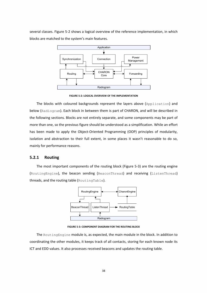
38

several classes. Figure 5-2 shows a logical overview of the reference implementation, in which

blocks are matched to the system’s main features.

FIGURE 5-2: LOGICAL OVERVIEW OF THE IMPLEMENTATION

The blocks with coloured backgrounds represent the layers above (Application) and

below (Radiogram). Each block in between them is part of CHARON, and will be described in

the following sections. Blocks are not entirely separate, and some components may be part of

more than one, so the previous figure should be understood as a simplification. While an effort

has been made to apply the Object-Oriented Programming (OOP) principles of modularity,

isolation and abstraction to their full extent, in some places it wasn’t reasonable to do so,

mainly for performance reasons.

5.2.1 Routing

The most important components of the routing block (Figure 5-3) are the routing engine

(RoutingEngine), the beacon sending (BeaconThread) and receiving (ListenThread)

threads, and the routing table (RoutingTable).

FIGURE 5-3: COMPONENT DIAGRAM FOR THE ROUTING BLOCK

The RoutingEngine module is, as expected, the main module in the block. In addition to

coordinating the other modules, it keeps track of all contacts, storing for each known node its

ICT and EDD values. It also processes received beacons and updates the routing table.

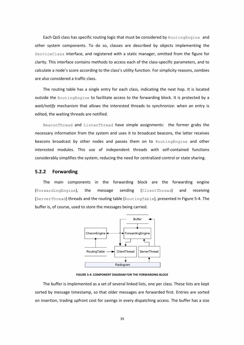
39

Each QoS class has specific routing logic that must be considered by RoutingEngine and

other system components. To do so, classes are described by objects implementing the

ServiceClass interface, and registered with a static manager, omitted from the figure for

clarity. This interface contains methods to access each of the class-specific parameters, and to

calculate a node’s score according to the class’s utility function. For simplicity reasons, zombies

are also considered a traffic class.

The routing table has a single entry for each class, indicating the next hop. It is located

outside the RoutingEngine to facilitate access to the forwarding block. It is protected by a

wait/notify mechanism that allows the interested threads to synchronize: when an entry is

edited, the waiting threads are notified.

BeaconThread and ListenThread have simple assignments: the former grabs the

necessary information from the system and uses it to broadcast beacons, the latter receives

beacons broadcast by other nodes and passes them on to RoutingEngine and other

interested modules. This use of independent threads with self-contained functions

considerably simplifies the system, reducing the need for centralized control or state sharing.

5.2.2 Forwarding

The main components in the forwarding block are the forwarding engine

(ForwardingEngine), the message sending (ClientThread) and receiving

(ServerThread) threads and the routing table (RoutingTable), presented in Figure 5-4. The

buffer is, of course, used to store the messages being carried.

FIGURE 5-4: COMPONENT DIAGRAM FOR THE FORWARDING BLOCK

The buffer is implemented as a set of several linked lists, one per class. These lists are kept

sorted by message timestamp, so that older messages are forwarded first. Entries are sorted

on insertion, trading upfront cost for savings in every dispatching access. The buffer has a size

40

limit, defined as a number of messages, which is freely distributed among classes. In order to

reduce the load on the garbage collector, all the list nodes are created on start-up and kept in

a shared pool4. Cleanups are periodically executed to remove expired messages and, if buffer

space goes under a specified limit, zombies (which are non-critical) are deleted to make room

for other messages.

ServerThread continuously waits for messages to be received and adds them to the

buffer, while ClientThread blocks on RoutingTable’s wait/notify mechanism. When the

table is updated, the thread wakes up and matches available routes to available queues,

starting with the highest priority class5. As soon as it finds a route for which there are

messages to send, it begins transmission. When all messages in that class have been

forwarded, it moves to the next class. This means, in effect, that while high-priority messages

are queued and a suitable round is available, lower-priority classes are not served. Starvation

of low-priority queues is possible if many high-priority classes are carried, but the system has

not been designed for such usage patterns. If a transmission fails, the message is put back into

the buffer. If a message’s class uses zombies, the message is moved to the zombie queue after

being sent. The thread performs a short sleep between each transmission as a way to throttle

resource and bandwidth occupation and allow more critical functions to execute. For instance,

by imposing non-transmission periods, channel access contention is reduced and beacon

messages suffer lower contention delays, improving synchronization precision.

In case the buffer fills up, message reception must be halted. That only takes place when

the node broadcasts the following beacon, advertising the lack of available memory. However,

before that occurs, messages may still be forwarded by other nodes. The obvious solution

would be to close the listening connection, resulting in acknowledgements not being sent, and

causing the sending nodes to stop. However, an optimization on the lower levels of the SPOT

stack leads to closed connections still acknowledging received messages, forestalling this

approach. This problem was solved by attaching the free buffer space to each routing entry.

This value is decremented by the node every time a message is sent. Because there may be

other nodes transmitting to the same destination, the announced buffer space should not be

4 In the absence of the shared pool, new list objects be would be allocated every time a message was received, requiring the garbage collector to remove these objects when the message was later forwarded, and wasting CPU cycles. 5 The concept of class priority wasn’t previously discussed as it is implementation-specific and not a design choice. Each class is assigned an integer that defines the order in which it is served. Urgent data should be configured with the highest priority level, while zombies should receive the lowest.

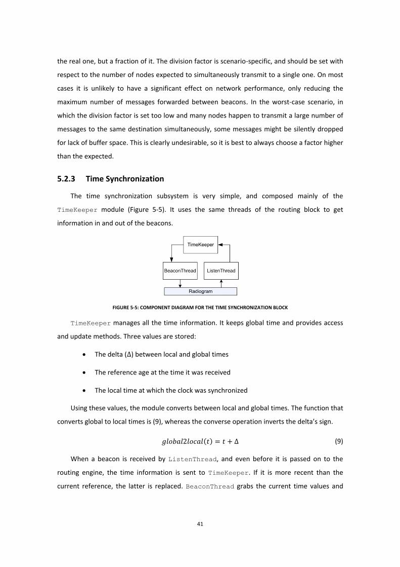
41

the real one, but a fraction of it. The division factor is scenario-specific, and should be set with

respect to the number of nodes expected to simultaneously transmit to a single one. On most

cases it is unlikely to have a significant effect on network performance, only reducing the

maximum number of messages forwarded between beacons. In the worst-case scenario, in

which the division factor is set too low and many nodes happen to transmit a large number of

messages to the same destination simultaneously, some messages might be silently dropped

for lack of buffer space. This is clearly undesirable, so it is best to always choose a factor higher

than the expected.

5.2.3 Time Synchronization

The time synchronization subsystem is very simple, and composed mainly of the

TimeKeeper module (Figure 5-5). It uses the same threads of the routing block to get

information in and out of the beacons.

FIGURE 5-5: COMPONENT DIAGRAM FOR THE TIME SYNCHRONIZATION BLOCK

TimeKeeper manages all the time information. It keeps global time and provides access

and update methods. Three values are stored:

The delta (Δ) between local and global times

The reference age at the time it was received

The local time at which the clock was synchronized

Using these values, the module converts between local and global times. The function that

converts global to local times is (9), whereas the converse operation inverts the delta’s sign.

𝑔𝑙𝑜𝑏𝑎𝑙2𝑙𝑜𝑐𝑎𝑙 𝑡 = 𝑡 + Δ (9)

When a beacon is received by ListenThread, and even before it is passed on to the

routing engine, the time information is sent to TimeKeeper. If it is more recent than the

current reference, the latter is replaced. BeaconThread grabs the current time values and

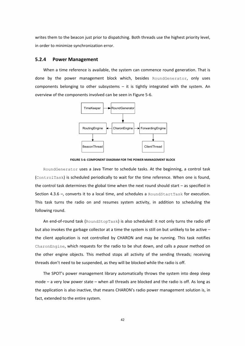
42

writes them to the beacon just prior to dispatching. Both threads use the highest priority level,

in order to minimize synchronization error.

5.2.4 Power Management

When a time reference is available, the system can commence round generation. That is

done by the power management block which, besides RoundGenerator, only uses

components belonging to other subsystems – it is tightly integrated with the system. An

overview of the components involved can be seen in Figure 5-6.

FIGURE 5-6: COMPONENT DIAGRAM FOR THE POWER MANAGEMENT BLOCK

RoundGenerator uses a Java Timer to schedule tasks. At the beginning, a control task

(ControlTask) is scheduled periodically to wait for the time reference. When one is found,

the control task determines the global time when the next round should start – as specified in

Section 4.3.6 –, converts it to a local time, and schedules a RoundStartTask for execution.

This task turns the radio on and resumes system activity, in addition to scheduling the

following round.

An end-of-round task (RoundStopTask) is also scheduled: it not only turns the radio off

but also invokes the garbage collector at a time the system is still on but unlikely to be active –

the client application is not controlled by CHARON and may be running. This task notifies

CharonEngine, which requests for the radio to be shut down, and calls a pause method on

the other engine objects. This method stops all activity of the sending threads; receiving

threads don’t need to be suspended, as they will be blocked while the radio is off.

The SPOT’s power management library automatically throws the system into deep sleep

mode – a very low power state – when all threads are blocked and the radio is off. As long as

the application is also inactive, that means CHARON’s radio power management solution is, in

fact, extended to the entire system.

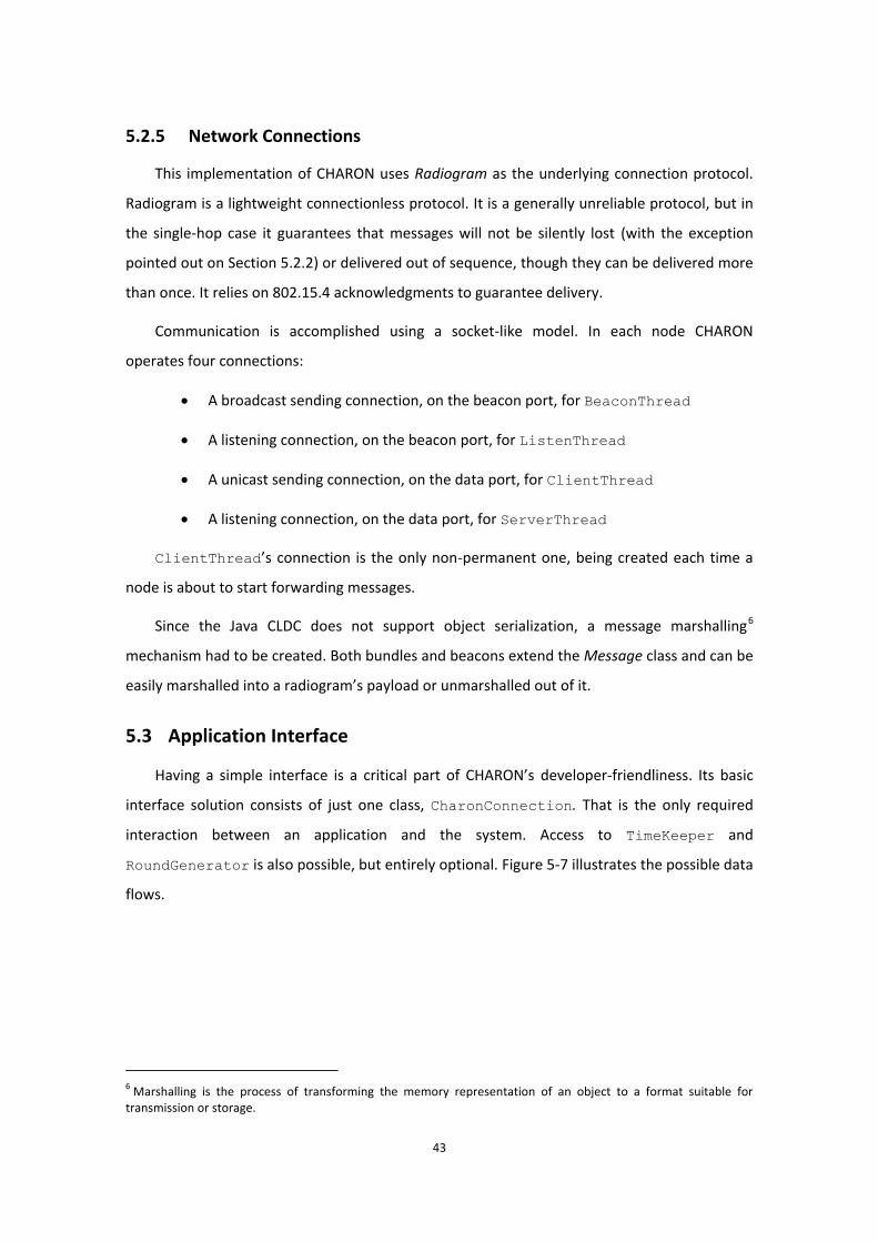
43

5.2.5 Network Connections

This implementation of CHARON uses Radiogram as the underlying connection protocol.

Radiogram is a lightweight connectionless protocol. It is a generally unreliable protocol, but in

the single-hop case it guarantees that messages will not be silently lost (with the exception

pointed out on Section 5.2.2) or delivered out of sequence, though they can be delivered more

than once. It relies on 802.15.4 acknowledgments to guarantee delivery.

Communication is accomplished using a socket-like model. In each node CHARON

operates four connections:

A broadcast sending connection, on the beacon port, for BeaconThread

A listening connection, on the beacon port, for ListenThread

A unicast sending connection, on the data port, for ClientThread

A listening connection, on the data port, for ServerThread

ClientThread’s connection is the only non-permanent one, being created each time a

node is about to start forwarding messages.

Since the Java CLDC does not support object serialization, a message marshalling6

mechanism had to be created. Both bundles and beacons extend the Message class and can be

easily marshalled into a radiogram’s payload or unmarshalled out of it.

5.3 Application Interface

Having a simple interface is a critical part of CHARON’s developer-friendliness. Its basic

interface solution consists of just one class, CharonConnection. That is the only required

interaction between an application and the system. Access to TimeKeeper and

RoundGenerator is also possible, but entirely optional. Figure 5-7 illustrates the possible data

flows.

6 Marshalling is the process of transforming the memory representation of an object to a format suitable for transmission or storage.

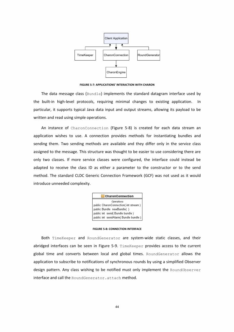
44

FIGURE 5-7: APPLICATIONS’ INTERACTION WITH CHARON

The data message class (Bundle) implements the standard datagram interface used by

the built-in high-level protocols, requiring minimal changes to existing application. In

particular, it supports typical Java data input and output streams, allowing its payload to be

written and read using simple operations.

An instance of CharonConnection (Figure 5-8) is created for each data stream an

application wishes to use. A connection provides methods for instantiating bundles and

sending them. Two sending methods are available and they differ only in the service class

assigned to the message. This structure was thought to be easier to use considering there are

only two classes. If more service classes were configured, the interface could instead be

adapted to receive the class ID as either a parameter to the constructor or to the send

method. The standard CLDC Generic Connection Framework (GCF) was not used as it would

introduce unneeded complexity.

FIGURE 5-8: CONNECTION INTERFACE

Both TimeKeeper and RoundGenerator are system-wide static classes, and their

abridged interfaces can be seen in Figure 5-9. TimeKeeper provides access to the current

global time and converts between local and global times. RoundGenerator allows the

application to subscribe to notifications of synchronous rounds by using a simplified Observer

design pattern. Any class wishing to be notified must only implement the RoundObserver

interface and call the RoundGenerator.attach method.

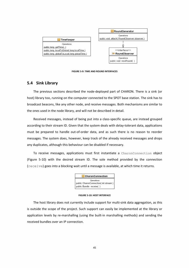
45

FIGURE 5-9: TIME AND ROUND INTERFACES

5.4 Sink Library

The previous sections described the node-deployed part of CHARON. There is a sink (or

host) library too, running on the computer connected to the SPOT base station. The sink has to

broadcast beacons, like any other node, and receive messages. Both mechanisms are similar to

the ones used in the node library, and will not be described in detail.

Received messages, instead of being put into a class-specific queue, are instead grouped

according to their stream ID. Given that the system deals with delay-tolerant data, applications

must be prepared to handle out-of-order data, and as such there is no reason to reorder

messages. The system does, however, keep track of the already received messages and drops

any duplicates, although this behaviour can be disabled if necessary.

To receive messages, applications must first instantiate a CharonConnection object

(Figure 5-10) with the desired stream ID. The sole method provided by the connection

(receive) goes into a blocking wait until a message is available, at which time it returns.

FIGURE 5-10: HOST INTERFACE

The host library does not currently include support for multi-sink data aggregation, as this

is outside the scope of the project. Such support can easily be implemented at the library or

application levels by re-marshalling (using the built-in marshalling methods) and sending the

received bundles over an IP connection.

46

5.5 Implementation Complexity

One of the goals set for CHARON was its ease of implementation, and verifying it was also

one of the reasons leading to the development of this prototype. While ease of

implementation is always a topic of subjective evaluation, some objective metrics can be

presented.

The full implementation contains 32 classes and 1517 physical source lines of code (SLOC),

excluding utilities and debugging functionality. It was finished in one and a half months of part-

time work by a developer unfamiliar with the platform, while an experienced full-time

developer could probably have done it in less than two weeks. These development times

appear to be acceptable, considering the multiple problems CHARON solves.

Although very subjective, a short comparison can be made with TinyOS, considering the

implementation of a power management solution similar to the one used (although more

complex) by the same developer [34]. That implementation required more than one month of

work, in addition to an intermediate redesign, mainly because of the unfriendly and exotic

nature of the development environment.

The full compiled suite stands at 47 KB, a value that must be seen in the context of the

used framework and system. In effect, given that the system has 4 MB of available Flash

memory, CHARON’s footprint isn’t relevant. Unfortunately, runtime RAM and CPU usage could

not be quantified, as support for profiling is not yet implemented in the SPOT firmware.

47

6 Evaluation

In order to validate the ideas behind CHARON, and evaluate its performance, a set of

evaluation experiments were conducted. These include large-scale simulations to perform

asymptotic performance analysis and real-world validation, carried out using the reference

implementation. This chapter details the evaluation protocol and presents the obtained

results.

6.1 Metrics of Interest

Several metrics of interest can be defined for the evaluation of CHARON. Considering each

metric’s importance and the restrictions imposed by the platform used and the equipment

available, the following were chosen:

Routing

o Delivery ratio is defined as the number of unique delivered messages, divided

by the number of sent messages

o Message latency measures the elapsed time between the creation of a

message by the source and the moment when it is first delivered to the

destination

o Hop count or path length is the number of hops a delivered message travels

through before reaching the sink

o Routing overhead describes the number of extraneous message transmissions,

i.e. those beyond the single required transmission from source to destination

Time synchronization

o Clock offset is the difference between two clocks carrying the same reference

o Clock drift is the rate at which the offset increases with time

Power management

o Node lifetime is the time required for a node’s battery to go from fully charged

to fully discharged

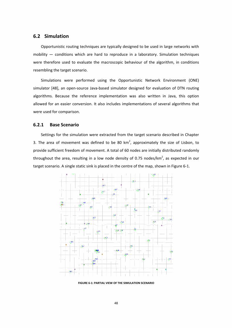
48

6.2 Simulation

Opportunistic routing techniques are typically designed to be used in large networks with

mobility — conditions which are hard to reproduce in a laboratory. Simulation techniques

were therefore used to evaluate the macroscopic behaviour of the algorithm, in conditions

resembling the target scenario.

Simulations were performed using the Opportunistic Network Environment (ONE)

simulator [48], an open-source Java-based simulator designed for evaluation of DTN routing

algorithms. Because the reference implementation was also written in Java, this option

allowed for an easier conversion. It also includes implementations of several algorithms that

were used for comparison.

6.2.1 Base Scenario

Settings for the simulation were extracted from the target scenario described in Chapter

3. The area of movement was defined to be 80 km2, approximately the size of Lisbon, to

provide sufficient freedom of movement. A total of 60 nodes are initially distributed randomly

throughout the area, resulting in a low node density of 0.75 nodes/km2, as expected in our

target scenario. A single static sink is placed in the centre of the map, shown in Figure 6-1.

FIGURE 6-1: PARTIAL VIEW OF THE SIMULATION SCENARIO

49

There are six node groups, emulating a setting where different species or populations

cohabit and exhibit different behaviour. Each group has a set of pre-defined waypoints, from

which nodes select their next destination. Movement speed is randomly chosen from a

predefined range (1.8 km/h to 18 km/h). Upon reaching a waypoint, nodes stop for a random

length of time (0 s to 120 s). Nodes of some groups can never come in direct contact with the

sink, as their movement area does not include the centre of the map. In the simulator used,

this model of waypoint pools is not compatible with unrestricted movement. Instead, an

approximation was implemented, in which nodes move on a tight lattice of possible paths,

using a shortest path algorithm to reach their destination.

Each node generates fixed-size messages (200 B of raw physical layer data) with fixed

periodicity (60 s). All nodes have 200 kB of buffer space, a reasonable size for current memory

capacities. All messages have the sink as their destination. A single sink was used to allow fair

comparison to protocols that don’t support more than one. Radio range (40 m) and bitrate

(250 kb/s) were chosen to reflect typical values for 802.15.4 [43] radios used in WSNs.

Each simulation runs for a period of 1 simulation day, during which 1440 messages are

generated. Movement and event generation are regulated by a pseudorandom number

generator. The generator seed is the same for multiple settings within each run, guaranteeing

comparable results.

Table 6-1 presents a summary of the already listed simulation parameters. These default

parameters are used in all simulations, except where otherwise noted.

TABLE 6-1: DEFAULT SIMULATION PARAMETERS

Area 80 km2

Number of nodes 60

Run duration 1 d

Radio range 40 m

Radio bit rate 250 kb/s

Buffer space 200 kB

Movement speed 1.8 km/h to 18 km/h

Idle movement time 0 s to 120 s

Message generation interval 60 s

Message size 200 B

Several of the simulation parameters may seem excessive, namely the message periodicity

and the movement speed. These were chosen in order to guarantee meaningful results in

simulations as short as 1 day, a necessity given the (real) time constraints for the evaluation.

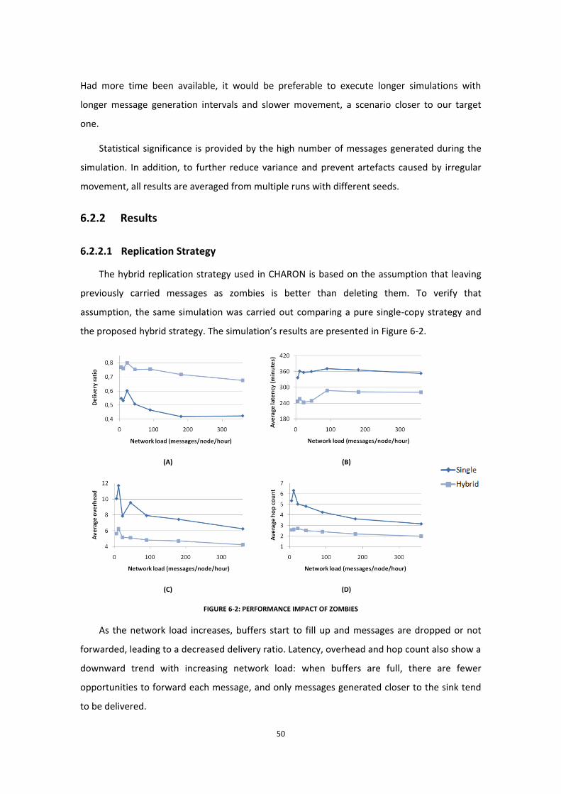
50

Had more time been available, it would be preferable to execute longer simulations with

longer message generation intervals and slower movement, a scenario closer to our target

one.

Statistical significance is provided by the high number of messages generated during the

simulation. In addition, to further reduce variance and prevent artefacts caused by irregular

movement, all results are averaged from multiple runs with different seeds.

6.2.2 Results

6.2.2.1 Replication Strategy

The hybrid replication strategy used in CHARON is based on the assumption that leaving

previously carried messages as zombies is better than deleting them. To verify that

assumption, the same simulation was carried out comparing a pure single-copy strategy and

the proposed hybrid strategy. The simulation’s results are presented in Figure 6-2.

(A)

(B)

(C)

(D)

FIGURE 6-2: PERFORMANCE IMPACT OF ZOMBIES

As the network load increases, buffers start to fill up and messages are dropped or not

forwarded, leading to a decreased delivery ratio. Latency, overhead and hop count also show a

downward trend with increasing network load: when buffers are full, there are fewer

opportunities to forward each message, and only messages generated closer to the sink tend

to be delivered.

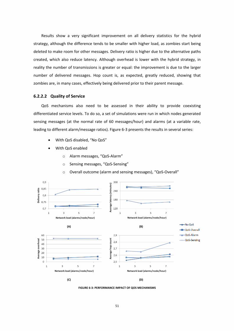
51

Results show a very significant improvement on all delivery statistics for the hybrid

strategy, although the difference tends to be smaller with higher load, as zombies start being

deleted to make room for other messages. Delivery ratio is higher due to the alternative paths

created, which also reduce latency. Although overhead is lower with the hybrid strategy, in

reality the number of transmissions is greater or equal: the improvement is due to the larger

number of delivered messages. Hop count is, as expected, greatly reduced, showing that

zombies are, in many cases, effectively being delivered prior to their parent message.

6.2.2.2 Quality of Service

QoS mechanisms also need to be assessed in their ability to provide coexisting

differentiated service levels. To do so, a set of simulations were run in which nodes generated

sensing messages (at the normal rate of 60 messages/hour) and alarms (at a variable rate,

leading to different alarm/message ratios). Figure 6-3 presents the results in several series:

With QoS disabled, “No QoS”

With QoS enabled

o Alarm messages, “QoS-Alarm”

o Sensing messages, “QoS-Sensing”

o Overall outcome (alarm and sensing messages), “QoS-Overall”

(A)

(B)

(C)

(D)

FIGURE 6-3: PERFORMANCE IMPACT OF QOS MECHANISMS

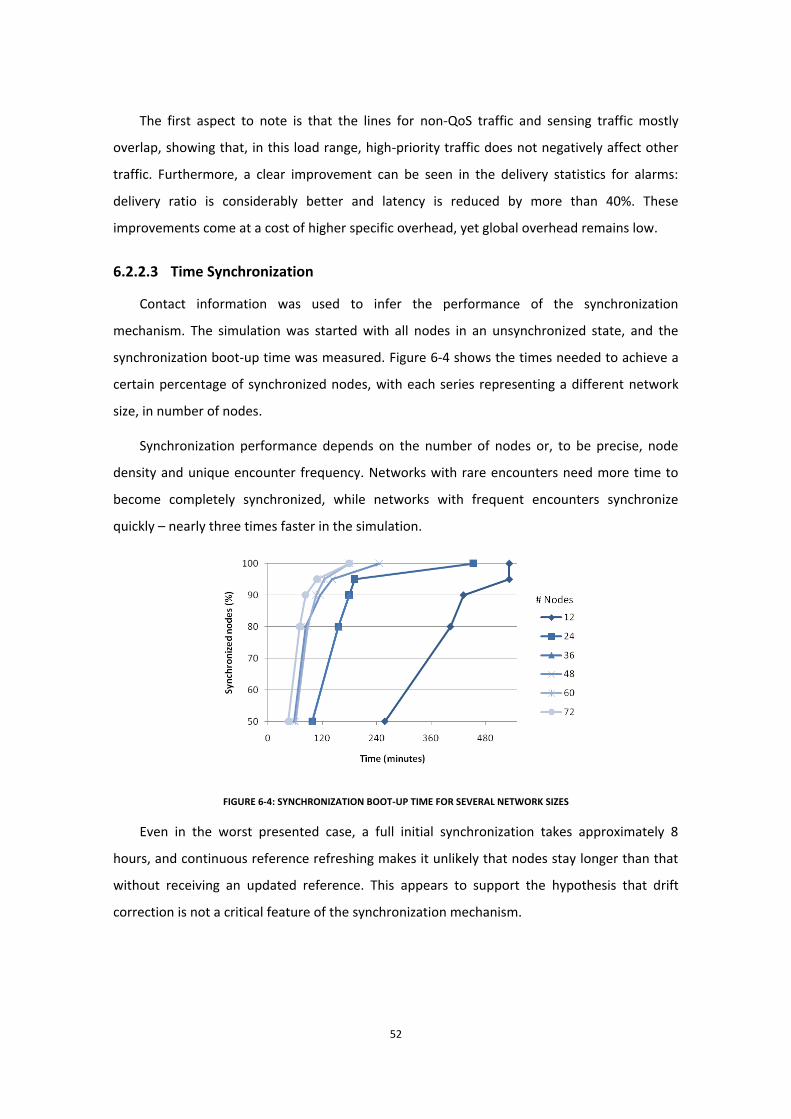
52

The first aspect to note is that the lines for non-QoS traffic and sensing traffic mostly

overlap, showing that, in this load range, high-priority traffic does not negatively affect other

traffic. Furthermore, a clear improvement can be seen in the delivery statistics for alarms:

delivery ratio is considerably better and latency is reduced by more than 40%. These

improvements come at a cost of higher specific overhead, yet global overhead remains low.

6.2.2.3 Time Synchronization

Contact information was used to infer the performance of the synchronization

mechanism. The simulation was started with all nodes in an unsynchronized state, and the

synchronization boot-up time was measured. Figure 6-4 shows the times needed to achieve a

certain percentage of synchronized nodes, with each series representing a different network

size, in number of nodes.

Synchronization performance depends on the number of nodes or, to be precise, node

density and unique encounter frequency. Networks with rare encounters need more time to

become completely synchronized, while networks with frequent encounters synchronize

quickly – nearly three times faster in the simulation.

FIGURE 6-4: SYNCHRONIZATION BOOT-UP TIME FOR SEVERAL NETWORK SIZES

Even in the worst presented case, a full initial synchronization takes approximately 8

hours, and continuous reference refreshing makes it unlikely that nodes stay longer than that

without receiving an updated reference. This appears to support the hypothesis that drift

correction is not a critical feature of the synchronization mechanism.

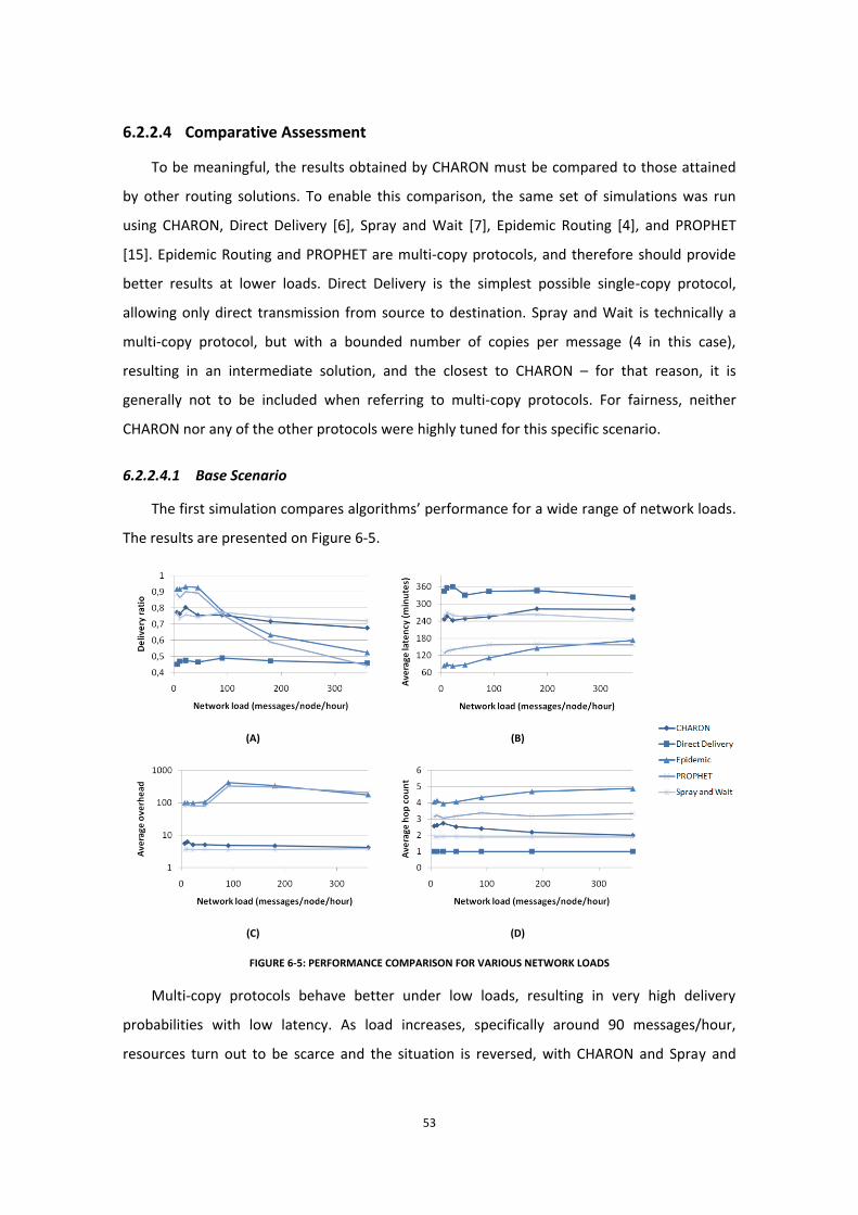
53

6.2.2.4 Comparative Assessment

To be meaningful, the results obtained by CHARON must be compared to those attained

by other routing solutions. To enable this comparison, the same set of simulations was run

using CHARON, Direct Delivery [6], Spray and Wait [7], Epidemic Routing [4], and PROPHET

[15]. Epidemic Routing and PROPHET are multi-copy protocols, and therefore should provide

better results at lower loads. Direct Delivery is the simplest possible single-copy protocol,

allowing only direct transmission from source to destination. Spray and Wait is technically a

multi-copy protocol, but with a bounded number of copies per message (4 in this case),

resulting in an intermediate solution, and the closest to CHARON – for that reason, it is

generally not to be included when referring to multi-copy protocols. For fairness, neither

CHARON nor any of the other protocols were highly tuned for this specific scenario.

6.2.2.4.1 Base Scenario

The first simulation compares algorithms’ performance for a wide range of network loads.

The results are presented on Figure 6-5.

(A)

(B)

(C)

(D)

FIGURE 6-5: PERFORMANCE COMPARISON FOR VARIOUS NETWORK LOADS

Multi-copy protocols behave better under low loads, resulting in very high delivery

probabilities with low latency. As load increases, specifically around 90 messages/hour,

resources turn out to be scarce and the situation is reversed, with CHARON and Spray and

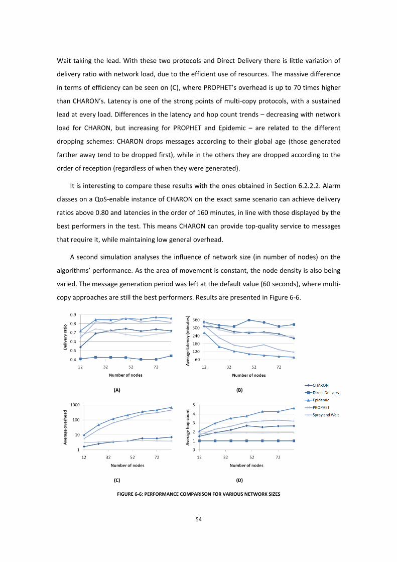
54

Wait taking the lead. With these two protocols and Direct Delivery there is little variation of

delivery ratio with network load, due to the efficient use of resources. The massive difference

in terms of efficiency can be seen on (C), where PROPHET’s overhead is up to 70 times higher

than CHARON’s. Latency is one of the strong points of multi-copy protocols, with a sustained

lead at every load. Differences in the latency and hop count trends – decreasing with network

load for CHARON, but increasing for PROPHET and Epidemic – are related to the different

dropping schemes: CHARON drops messages according to their global age (those generated

farther away tend to be dropped first), while in the others they are dropped according to the

order of reception (regardless of when they were generated).

It is interesting to compare these results with the ones obtained in Section 6.2.2.2. Alarm

classes on a QoS-enable instance of CHARON on the exact same scenario can achieve delivery

ratios above 0.80 and latencies in the order of 160 minutes, in line with those displayed by the

best performers in the test. This means CHARON can provide top-quality service to messages

that require it, while maintaining low general overhead.

A second simulation analyses the influence of network size (in number of nodes) on the

algorithms’ performance. As the area of movement is constant, the node density is also being

varied. The message generation period was left at the default value (60 seconds), where multi-

copy approaches are still the best performers. Results are presented in Figure 6-6.

(A)

(B)

(C)

(D)

FIGURE 6-6: PERFORMANCE COMPARISON FOR VARIOUS NETWORK SIZES

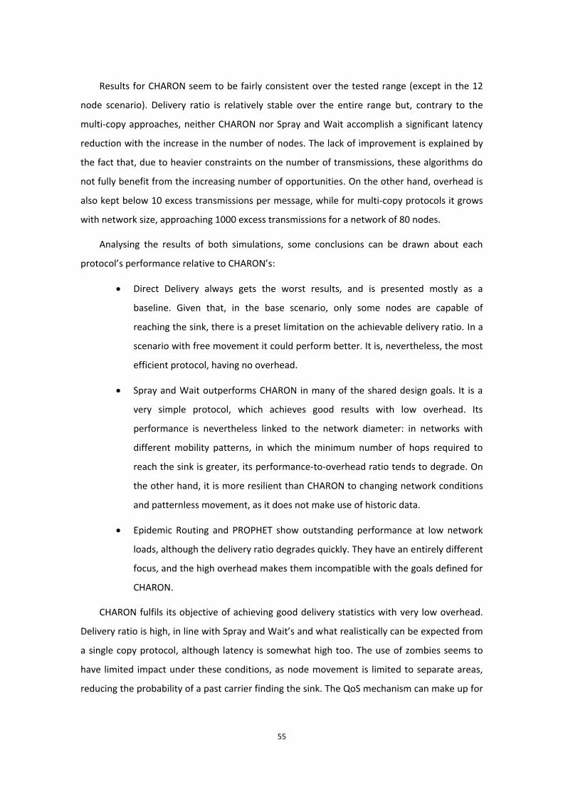
55

Results for CHARON seem to be fairly consistent over the tested range (except in the 12

node scenario). Delivery ratio is relatively stable over the entire range but, contrary to the

multi-copy approaches, neither CHARON nor Spray and Wait accomplish a significant latency

reduction with the increase in the number of nodes. The lack of improvement is explained by

the fact that, due to heavier constraints on the number of transmissions, these algorithms do

not fully benefit from the increasing number of opportunities. On the other hand, overhead is

also kept below 10 excess transmissions per message, while for multi-copy protocols it grows

with network size, approaching 1000 excess transmissions for a network of 80 nodes.

Analysing the results of both simulations, some conclusions can be drawn about each

protocol’s performance relative to CHARON’s:

Direct Delivery always gets the worst results, and is presented mostly as a

baseline. Given that, in the base scenario, only some nodes are capable of

reaching the sink, there is a preset limitation on the achievable delivery ratio. In a

scenario with free movement it could perform better. It is, nevertheless, the most

efficient protocol, having no overhead.

Spray and Wait outperforms CHARON in many of the shared design goals. It is a

very simple protocol, which achieves good results with low overhead. Its

performance is nevertheless linked to the network diameter: in networks with

different mobility patterns, in which the minimum number of hops required to

reach the sink is greater, its performance-to-overhead ratio tends to degrade. On

the other hand, it is more resilient than CHARON to changing network conditions

and patternless movement, as it does not make use of historic data.

Epidemic Routing and PROPHET show outstanding performance at low network

loads, although the delivery ratio degrades quickly. They have an entirely different

focus, and the high overhead makes them incompatible with the goals defined for

CHARON.

CHARON fulfils its objective of achieving good delivery statistics with very low overhead.

Delivery ratio is high, in line with Spray and Wait’s and what realistically can be expected from

a single copy protocol, although latency is somewhat high too. The use of zombies seems to

have limited impact under these conditions, as node movement is limited to separate areas,

reducing the probability of a past carrier finding the sink. The QoS mechanism can make up for

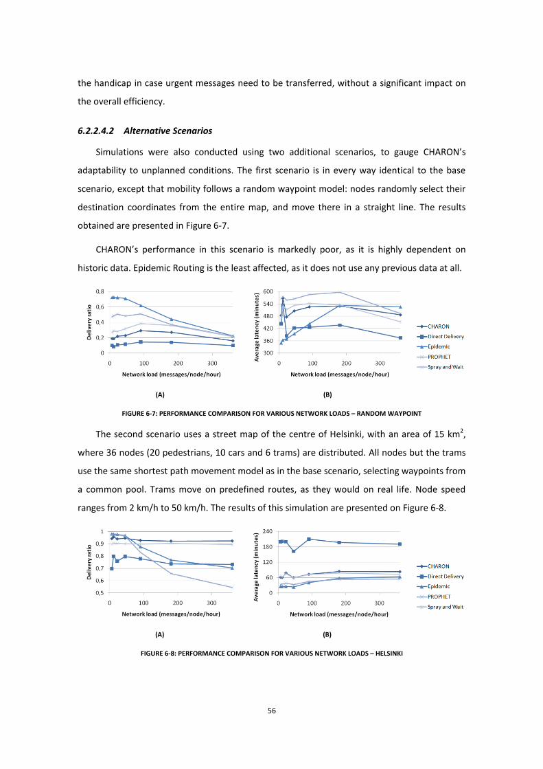
56

the handicap in case urgent messages need to be transferred, without a significant impact on

the overall efficiency.

6.2.2.4.2 Alternative Scenarios

Simulations were also conducted using two additional scenarios, to gauge CHARON’s

adaptability to unplanned conditions. The first scenario is in every way identical to the base

scenario, except that mobility follows a random waypoint model: nodes randomly select their

destination coordinates from the entire map, and move there in a straight line. The results

obtained are presented in Figure 6-7.

CHARON’s performance in this scenario is markedly poor, as it is highly dependent on

historic data. Epidemic Routing is the least affected, as it does not use any previous data at all.

(A)

(B)

FIGURE 6-7: PERFORMANCE COMPARISON FOR VARIOUS NETWORK LOADS – RANDOM WAYPOINT

The second scenario uses a street map of the centre of Helsinki, with an area of 15 km2,

where 36 nodes (20 pedestrians, 10 cars and 6 trams) are distributed. All nodes but the trams

use the same shortest path movement model as in the base scenario, selecting waypoints from

a common pool. Trams move on predefined routes, as they would on real life. Node speed

ranges from 2 km/h to 50 km/h. The results of this simulation are presented on Figure 6-8.

(A)

(B)

FIGURE 6-8: PERFORMANCE COMPARISON FOR VARIOUS NETWORK LOADS – HELSINKI

57

Contrary to the previous scenario, in this case CHARON leads in delivery ratio and achieves

good results for the average latency. Interestingly, CHARON’s performance is virtually

independent of the network load. The results are explained by the higher freedom of

movement – which potentiates the impact of zombies – combined with faster movement that

increases contact frequency and the accuracy of CHARON’s delay calculations.

6.3 Real-World Validation

The reference implementation of CHARON allowed testing under real-world conditions

and using real-world hardware. That testing includes the validation of all architectural

components, and a limited evaluation of the achieved performance, given the limited available

resources. Tests were conducted on a laboratory (workbench) setting and on an experimental

testbed.

6.3.1 Test Application

A basic test application was developed and used in most of the real-world tests. The

application creates a single connection with a network-wide common stream ID. It subscribes

to round events and, in each round, generates one or more messages. Each message contains

one temperature and one brightness sample, for a total of 8 bytes of data. Messages are sent

as monitoring data. Alarm data can be generated by pressing a button on the SPOT, but that

feature was not used in the tests, as it is practically impossible to evaluate QoS influence with

the available resources. Except where otherwise noted, nodes were configured with enough

buffer space for 100 messages and a beacon period of 500 ms.

6.3.2 Workbench Tests

A series of workbench tests were conducted to evaluate specific mechanisms on a static

setting. Four SPOT nodes and one sink (referred to interchangeably as base station) were used

for these tests.

6.3.2.1 Basic Tests

The basic tests were meant to verify that the algorithm and implementation were

correctly designed and working as expected. The following pass/fail tests were done:

Routing

o Beacon broadcast

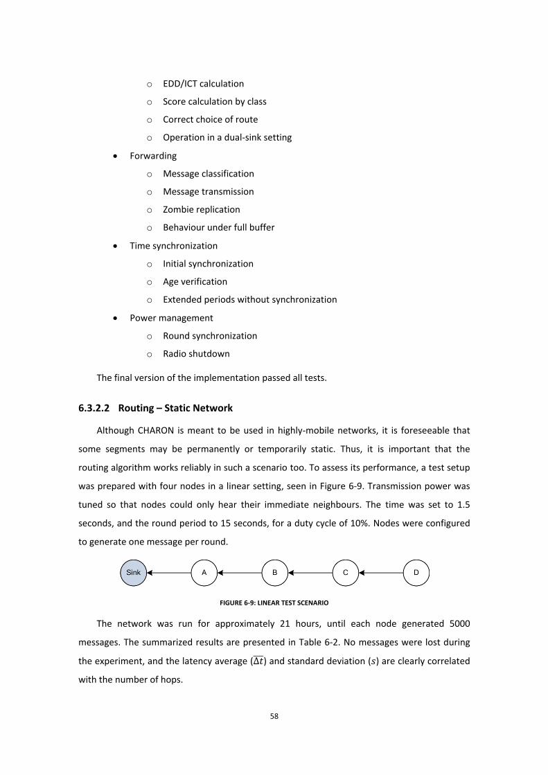
58

o EDD/ICT calculation

o Score calculation by class

o Correct choice of route

o Operation in a dual-sink setting

Forwarding

o Message classification

o Message transmission

o Zombie replication

o Behaviour under full buffer

Time synchronization

o Initial synchronization

o Age verification

o Extended periods without synchronization

Power management

o Round synchronization

o Radio shutdown

The final version of the implementation passed all tests.

6.3.2.2 Routing – Static Network

Although CHARON is meant to be used in highly-mobile networks, it is foreseeable that

some segments may be permanently or temporarily static. Thus, it is important that the

routing algorithm works reliably in such a scenario too. To assess its performance, a test setup

was prepared with four nodes in a linear setting, seen in Figure 6-9. Transmission power was

tuned so that nodes could only hear their immediate neighbours. The time was set to 1.5

seconds, and the round period to 15 seconds, for a duty cycle of 10%. Nodes were configured

to generate one message per round.

FIGURE 6-9: LINEAR TEST SCENARIO

The network was run for approximately 21 hours, until each node generated 5000

messages. The summarized results are presented in Table 6-2. No messages were lost during

the experiment, and the latency average (∆𝑡 ) and standard deviation (𝑠) are clearly correlated

with the number of hops.

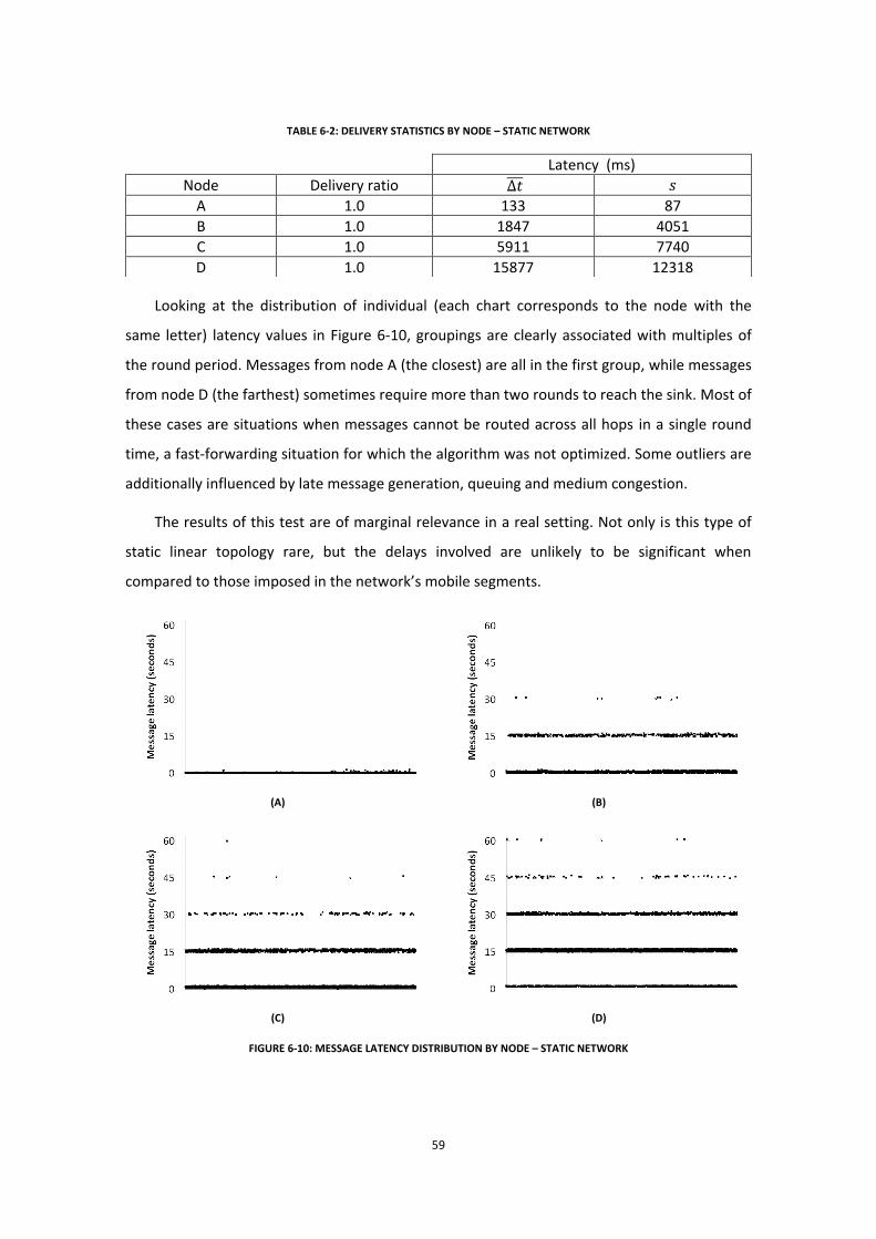
59

TABLE 6-2: DELIVERY STATISTICS BY NODE – STATIC NETWORK

Latency (ms)

Node Delivery ratio ∆𝑡 𝑠

A 1.0 133 87

B 1.0 1847 4051

C 1.0 5911 7740

D 1.0 15877 12318

Looking at the distribution of individual (each chart corresponds to the node with the

same letter) latency values in Figure 6-10, groupings are clearly associated with multiples of

the round period. Messages from node A (the closest) are all in the first group, while messages

from node D (the farthest) sometimes require more than two rounds to reach the sink. Most of

these cases are situations when messages cannot be routed across all hops in a single round

time, a fast-forwarding situation for which the algorithm was not optimized. Some outliers are

additionally influenced by late message generation, queuing and medium congestion.

The results of this test are of marginal relevance in a real setting. Not only is this type of

static linear topology rare, but the delays involved are unlikely to be significant when

compared to those imposed in the network’s mobile segments.

(A)

(B)

(C)

(D)

FIGURE 6-10: MESSAGE LATENCY DISTRIBUTION BY NODE – STATIC NETWORK

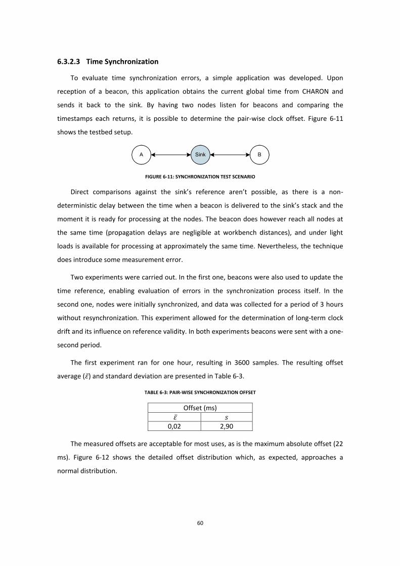
60

6.3.2.3 Time Synchronization

To evaluate time synchronization errors, a simple application was developed. Upon

reception of a beacon, this application obtains the current global time from CHARON and

sends it back to the sink. By having two nodes listen for beacons and comparing the

timestamps each returns, it is possible to determine the pair-wise clock offset. Figure 6-11

shows the testbed setup.

FIGURE 6-11: SYNCHRONIZATION TEST SCENARIO

Direct comparisons against the sink’s reference aren’t possible, as there is a non-

deterministic delay between the time when a beacon is delivered to the sink’s stack and the

moment it is ready for processing at the nodes. The beacon does however reach all nodes at

the same time (propagation delays are negligible at workbench distances), and under light

loads is available for processing at approximately the same time. Nevertheless, the technique

does introduce some measurement error.

Two experiments were carried out. In the first one, beacons were also used to update the

time reference, enabling evaluation of errors in the synchronization process itself. In the

second one, nodes were initially synchronized, and data was collected for a period of 3 hours

without resynchronization. This experiment allowed for the determination of long-term clock

drift and its influence on reference validity. In both experiments beacons were sent with a one-

second period.

The first experiment ran for one hour, resulting in 3600 samples. The resulting offset

average (휀 ) and standard deviation are presented in Table 6-3.

TABLE 6-3: PAIR-WISE SYNCHRONIZATION OFFSET

Offset (ms)

휀 𝑠 0,02 2,90

The measured offsets are acceptable for most uses, as is the maximum absolute offset (22

ms). Figure 6-12 shows the detailed offset distribution which, as expected, approaches a

normal distribution.

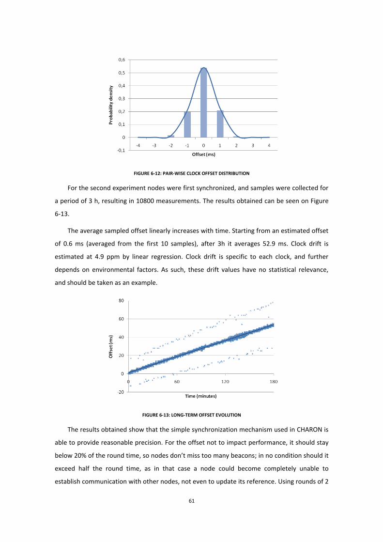
61

FIGURE 6-12: PAIR-WISE CLOCK OFFSET DISTRIBUTION

For the second experiment nodes were first synchronized, and samples were collected for

a period of 3 h, resulting in 10800 measurements. The results obtained can be seen on Figure

6-13.

The average sampled offset linearly increases with time. Starting from an estimated offset

of 0.6 ms (averaged from the first 10 samples), after 3h it averages 52.9 ms. Clock drift is

estimated at 4.9 ppm by linear regression. Clock drift is specific to each clock, and further

depends on environmental factors. As such, these drift values have no statistical relevance,

and should be taken as an example.

FIGURE 6-13: LONG-TERM OFFSET EVOLUTION

The results obtained show that the simple synchronization mechanism used in CHARON is

able to provide reasonable precision. For the offset not to impact performance, it should stay

below 20% of the round time, so nodes don’t miss too many beacons; in no condition should it

exceed half the round time, as in that case a node could become completely unable to

establish communication with other nodes, not even to update its reference. Using rounds of 2

62

seconds and the measured offset and drift values, a node would require one full day to drift

more than 20%, and 2.3 days to drift 50%.

6.3.2.4 Power Management

The influence of CHARON’s radio power management solution on the lifetime of nodes

was measured by having a fully-charged node run the test application in contact with a sink.

The sink recorded the arrival timestamp of every message, and the lifetime was extracted by

subtracting the first from the last timestamps. The round period was set to 20 seconds and the

round time was varied to achieve the duty cycles (𝜂) presented in Table 6-4.

FIGURE 6-14: POWER MANAGEMENT TEST SCENARIO

In the experiment conducted on Section 6.3.2.2 no strong connection was found between

the position the node occupies and its energy consumption. This is justified by the fact that, in

the SPOT platform, energy consumption is lower in transmit mode than in receive mode [44],

in which every node – regardless of its position – spends the majority of its round time. For this

reason, and considering the long time required for each experiment, no tests were run with

multiple nodes.

TABLE 6-4: NODE LIFETIME UNDER DIFFERENT POWER MANAGEMENT CONFIGURATIONS

𝜂 100% 70% 40% 10%

Lifetime (h) 14,63 18,00 28,35 79,71

Improvement +23% +94% +445%

The use of radio power management has a clear effect on the global energy consumption.

Not only is the radio turned off but, given that the entire library and the application itself are

synchronized to the rounds, nodes are free to enter deep sleep mode. While a SPOT node in a

fully active state has a power usage of up to 104 mA, in deep sleep it is reduced to just 33 µA,

an almost negligible value [49].

Figure 6-15 plots node lifetime as a function of the radio duty cycle, showing that it

follows a power law (with 𝑟2 = 0,999) on the range analysed. Extrapolating from these

results, a duty cycle of 1% would extend node lifetime to approximately 18 days, although the

available data points aren’t sufficient to ensure a high confidence level for this prediction.

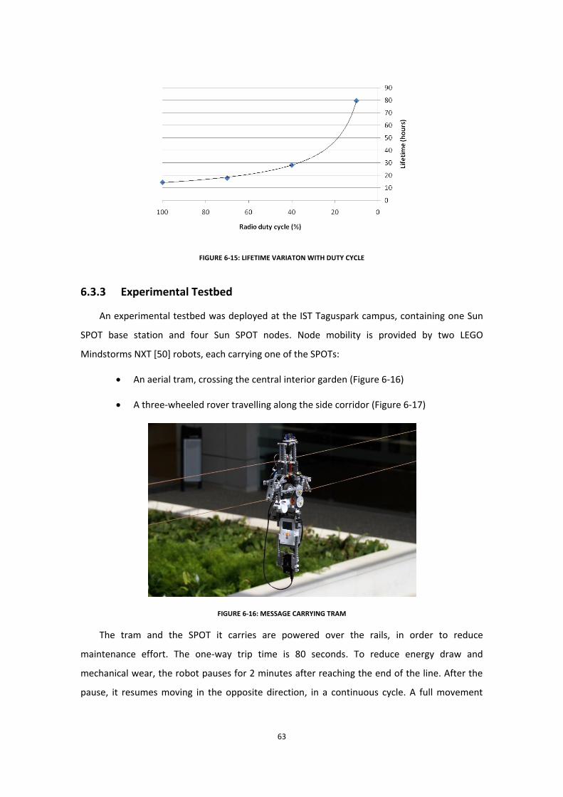
63

FIGURE 6-15: LIFETIME VARIATON WITH DUTY CYCLE

6.3.3 Experimental Testbed

An experimental testbed was deployed at the IST Taguspark campus, containing one Sun

SPOT base station and four Sun SPOT nodes. Node mobility is provided by two LEGO

Mindstorms NXT [50] robots, each carrying one of the SPOTs:

An aerial tram, crossing the central interior garden (Figure 6-16)

A three-wheeled rover travelling along the side corridor (Figure 6-17)

FIGURE 6-16: MESSAGE CARRYING TRAM

The tram and the SPOT it carries are powered over the rails, in order to reduce

maintenance effort. The one-way trip time is 80 seconds. To reduce energy draw and

mechanical wear, the robot pauses for 2 minutes after reaching the end of the line. After the

pause, it resumes moving in the opposite direction, in a continuous cycle. A full movement

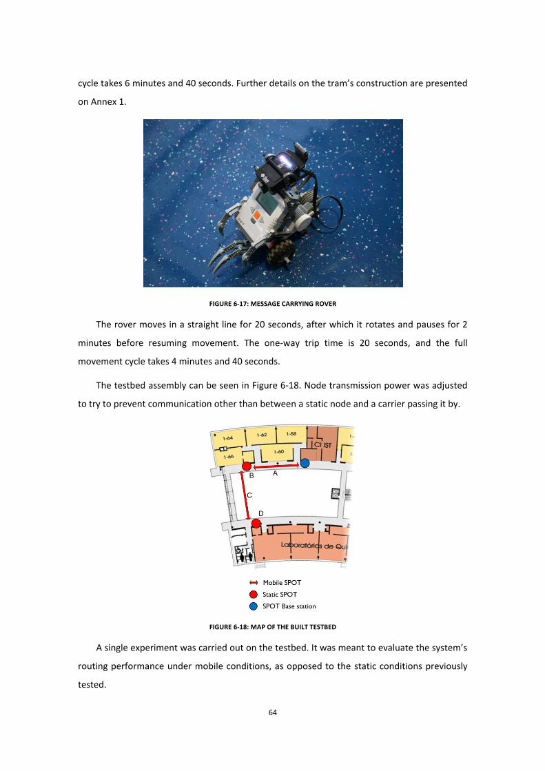
64

cycle takes 6 minutes and 40 seconds. Further details on the tram’s construction are presented

on Annex 1.

FIGURE 6-17: MESSAGE CARRYING ROVER

The rover moves in a straight line for 20 seconds, after which it rotates and pauses for 2

minutes before resuming movement. The one-way trip time is 20 seconds, and the full

movement cycle takes 4 minutes and 40 seconds.

The testbed assembly can be seen in Figure 6-18. Node transmission power was adjusted

to try to prevent communication other than between a static node and a carrier passing it by.

FIGURE 6-18: MAP OF THE BUILT TESTBED

A single experiment was carried out on the testbed. It was meant to evaluate the system’s

routing performance under mobile conditions, as opposed to the static conditions previously

tested.

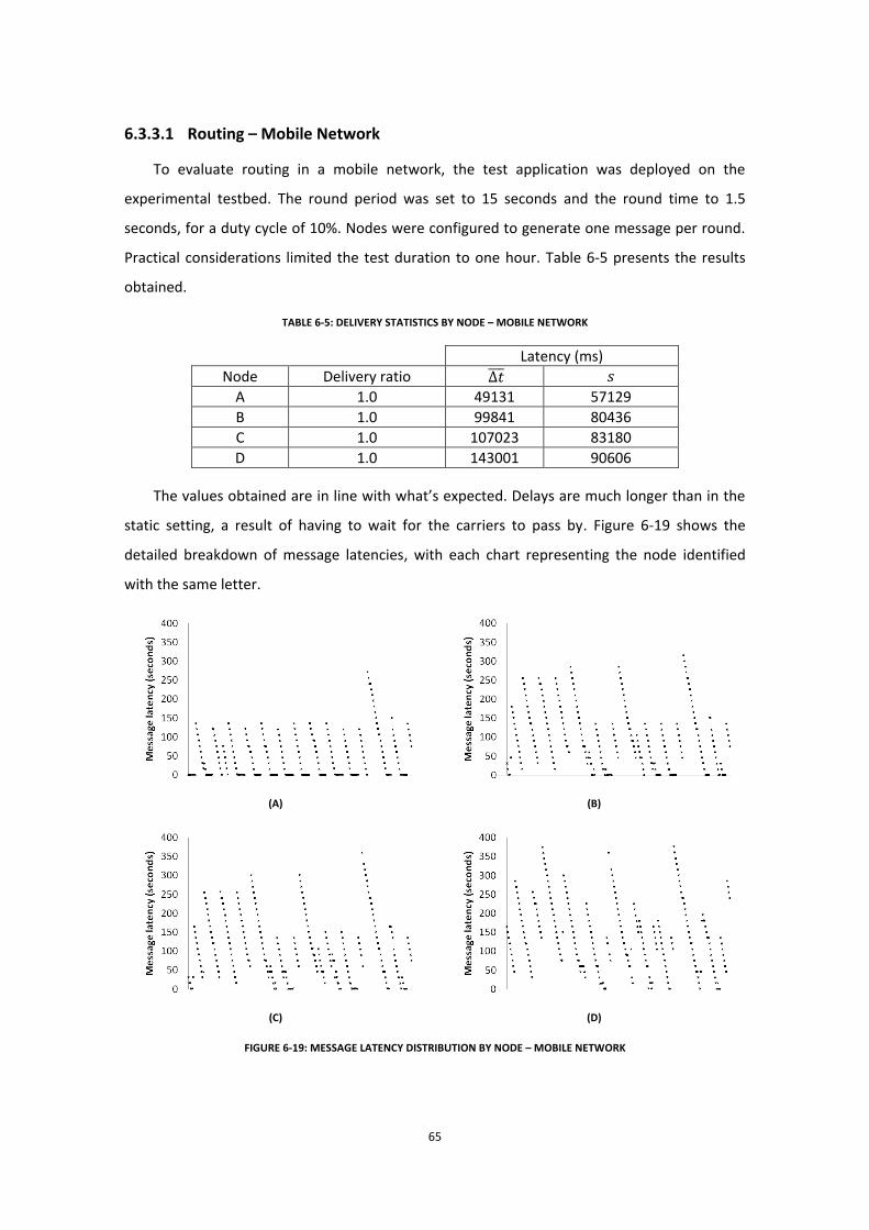
65

6.3.3.1 Routing – Mobile Network

To evaluate routing in a mobile network, the test application was deployed on the

experimental testbed. The round period was set to 15 seconds and the round time to 1.5

seconds, for a duty cycle of 10%. Nodes were configured to generate one message per round.

Practical considerations limited the test duration to one hour. Table 6-5 presents the results

obtained.

TABLE 6-5: DELIVERY STATISTICS BY NODE – MOBILE NETWORK

Latency (ms)

Node Delivery ratio ∆𝑡 𝑠

A 1.0 49131 57129

B 1.0 99841 80436

C 1.0 107023 83180

D 1.0 143001 90606

The values obtained are in line with what’s expected. Delays are much longer than in the

static setting, a result of having to wait for the carriers to pass by. Figure 6-19 shows the

detailed breakdown of message latencies, with each chart representing the node identified

with the same letter.

(A)

(B)

(C)

(D)

FIGURE 6-19: MESSAGE LATENCY DISTRIBUTION BY NODE – MOBILE NETWORK

66

Descending lines can be seen on every chart: they correspond to carrier trips. Messages

are created every round time, but their latency depends on the position of the carriers

involved at the time of generation. Specifically, if a message is generated by a carrier moving

towards the sink, its latency is inversely dependent on the distance between the carrier and its

destination. The farthest the node is from the sink, the longer these lines are.

The horizontal lines in node A’s chart correspond to the times in which the robot is parked

next to the sink and messages are delivered without mobility-imposed delay. According to the

defined scenario parameters, nodes should only be able to connect when in close proximity, so

these lines should not be present on other nodes’ charts. The fact that they are means that,

under specific conditions, communication range was long enough to create unexpected

connection opportunities. The main reason for this is the positioning of the aerial tram: owing

to the transmission power needed to overcome physical barriers present at close range, the

tram is occasionally able to communicate from farther points in its path across an open,

unobstructed area.

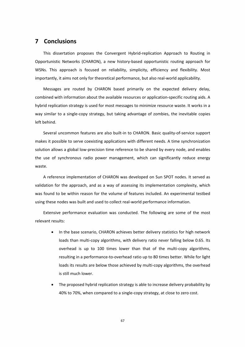
67

7 Conclusions

This dissertation proposes the Convergent Hybrid-replication Approach to Routing in

Opportunistic Networks (CHARON), a new history-based opportunistic routing approach for

WSNs. This approach is focused on reliability, simplicity, efficiency and flexibility. Most

importantly, it aims not only for theoretical performance, but also real-world applicability.

Messages are routed by CHARON based primarily on the expected delivery delay,

combined with information about the available resources or application-specific routing aids. A

hybrid replication strategy is used for most messages to minimize resource waste. It works in a

way similar to a single-copy strategy, but taking advantage of zombies, the inevitable copies

left behind.

Several uncommon features are also built-in to CHARON. Basic quality-of-service support

makes it possible to serve coexisting applications with different needs. A time synchronization

solution allows a global low-precision time reference to be shared by every node, and enables

the use of synchronous radio power management, which can significantly reduce energy

waste.

A reference implementation of CHARON was developed on Sun SPOT nodes. It served as

validation for the approach, and as a way of assessing its implementation complexity, which

was found to be within reason for the volume of features included. An experimental testbed

using these nodes was built and used to collect real-world performance information.

Extensive performance evaluation was conducted. The following are some of the most

relevant results:

In the base scenario, CHARON achieves better delivery statistics for high network

loads than multi-copy algorithms, with delivery ratio never falling below 0.65. Its

overhead is up to 100 times lower than that of the multi-copy algorithms,

resulting in a performance-to-overhead ratio up to 80 times better. While for light

loads its results are below those achieved by multi-copy algorithms, the overhead

is still much lower.

The proposed hybrid replication strategy is able to increase delivery probability by

40% to 70%, when compared to a single-copy strategy, at close to zero cost.

68

The proposed QoS mechanism is able to provide multi-copy-like performance on

urgent data, while routing non-urgent data with very low overhead.

The proposed synchronization mechanism is able to provide a useful global time

reference, with initial error in the single-digit milliseconds and, in the prototype

platform, maintain valid references for over two days.

The proposed power management mechanism was able to increase the

prototype node’s lifetime by over 440% for a conservative 10% duty cycle.

The reference implementation was able to effectively route messages in an

experimental testbed, providing important but often-overlooked real-world

validation.

The results obtained show CHARON to be a valid approach to routing in opportunistic

WSNs, achieving good performance with low overhead. CHARON manages to accomplish and

balance the four goals initially set, providing an effective and efficient solution, that is also

flexible yet still simple to understand and implement.

7.1 Future Work

There are still several challenges and paths for improvement in future work.

Improvements do, however, have a tendency to increase a solution’s complexity, and a cost-

benefit analysis should be made prior to development. The following are some of the

remaining open issues:

More advanced uses of delay as a routing metric could be investigated and

merged into the protocol. Particularly, instead of focusing only on the shortest

known path, other redundant paths to sink nodes should be considered for the

final calculation.

Time synchronization is designed in the simplest possible way. This is one of the

areas where limited additional complexity may be desirable. While the achieved

precision is usually sufficient, it can be improved by accounting for some of the

delay factors. Furthermore, the algorithm could be made more resilient against

pathological cases, by considering several references instead of just the latest.

Integrating techniques for secure routing could prove useful as WSN usage

increases. At the routing level, an un-secured network allows an attacker to

69

perform basic denial-of-service attacks [51] by either announcing itself as a good

forwarder and black-holing traffic, or injecting traffic leading to buffer exhaustion.

Both problems may be solved by applying a message integrity code (MIC) to all

beacon and data messages. While Sybil attacks [52] are also prevented by this

mechanism, wormhole attacks [53] are still possible, as well as several non-

routing-specific attacks.

Collection of mobility information could prove helpful in many scenarios. Mobility

data could be extracted from a node’s previous contacts and periodically

forwarded to the sink, or a list of hops could be attached to each bundle.

Combined with geo-referenced static nodes, this mechanism could also provide

coarse location information, valuable in an animal-tracking scenario, for instance.

Deployment in a real WSN, followed by in-depth evaluation would, of course, be

extremely helpful in identifying CHARON’s usefulness in real-world scenarios. In

addition to providing real-world performance data for CHARON, it would also aid

in identifying weaknesses in the simulation methodology.

70

References

[1] A. S. Tanenbaum, C. Gamage, and B. Crispo, "Taking Sensor Networks from the Lab to the

Jungle," Computer, vol. 39, no. 8, pp. 98-100, Aug. 2006.

[2] L. Pelusi, A. Passarella, and M. Conti, "Opportunistic Networking: Data Forwarding in

Disconnected Mobile Ad Hoc Networks," IEEE Communications Magazine, vol. 44, no. 11,

pp. 134-141, Nov. 2006.

[3] Z. Zhang, "Routing in Intermittently Connected Mobile Ad Hoc Networks and Delay

Tolerant Networks: Overview and Challenges," IEEE Communications Surveys & Tutorials,

vol. 8, no. 1, pp. 24-37, Jan. 2006.

[4] A. Vahdat and D. Becker, "Epidemic Routing for Partially-Connected Ad Hoc Networks,"

Duke University, Durham, North Carolina, USA, Technical Report CS-2000-06, 2000.

[5] M. Grossglauser and D. N. C. Tse, "Mobility Increases the Capacity of Ad Hoc Wireless

Networks," IEEE/ACM Transactions on Networking, vol. 10, no. 4, pp. 477-486, Aug. 2002.

[6] T. Matsuda and T. Takine, "(p,q)-Epidemic Routing for Sparsely Populated Mobile Ad Hoc

Networks," IEEE Journal on Selected Areas in Communications, vol. 26, no. 5, pp. 783-793,

Jun. 2008.

[7] T. Spyropoulos, K. Psounis, and C. S. Raghavendra, "Spray and Wait: An Efficient Routing

Scheme for Intermittently Connected Mobile Networks," in Proceedings of the 2005 ACM

SIGCOMM Workshop on Delay-Tolerant Networking, Philadelphia, Pennsylvania, USA,

2005, pp. 252-259.

[8] F. Tchakountio and R. Ramanathan, "Tracking Highly Mobile Endpoints," in Proceedings of

the 4th ACM International Workshop on Wireless Mobile Multimedia, Rome, Italy, 2001,

pp. 83-94.

[9] D. J. Goodman, J. Borràs, N. B. Mandayam, and R. D. Yates, "INFOSTATIONS: A New

System Model for Data and Messaging Services," in IEEE 47th Vehicular Technology

Conference, Phoenix, Arizona, USA, 1997, pp. 969-973.

[10] T. Small and Z. J. Haas, "The Shared Wireless Infostation Model: A New Ad Hoc

Networking Paradigm (or Where There Is a Whale, There Is a Way)," in Proceedings of the

4th ACM International Symposium on Mobile Ad Hoc Networking & Computing, Annapolis,

71

Maryland, USA, 2003, pp. 233-244.

[11] R. C. Shah, S. Roy, S. Jain, and W. Brunette, "Data MULEs: Modeling a Three-Tier

Architecture for Sparse Sensor Networks," in Proceedings of the First IEEE International

Workshop on Sensor Network Protocols and Applications, Anchorage, Alaska, USA, 2003,

pp. 30-41.

[12] P. Juang, et al., "Energy-Efficient Computing for Wildlife Tracking: Design Tradeoffs and

Early Experiences with Zebranet," in Proceedings of the 10th International Conference on

Architectural Support for Programming Languages and Operating Systems, San Jose,

California, USA, 2002, pp. 96-107.

[13] P. Zhang, C. M. Sadler, S. A. Lyon, and M. Martonosi, "Hardware Design Experiences in

ZebraNet," in Proceedings of the 2nd International Conference on Embedded Networked

Sensor Systems, Baltimore, Maryland, USA, 2004, pp. 227-238.

[14] B. Burns, O. Brock, and B. N. Levine, "MV Routing and Capacity Building in Disruption

Tolerant Networks," in INFOCOM 2005. 24th Annual Joint Conference of the IEEE

Computer and Communications Societies, Miami, Florida, USA, 2005, pp. 398-408.

[15] A. Lindgren, A. Doria, and O. Schelén, "Probabilistic Routing in Intermittently Connected

Networks," ACM SIGMOBILE Mobile Computing and Communications Review, vol. 7, no. 3,

pp. 19-20, Jul. 2003.

[16] M. Musolesi, S. Hailes, and C. Mascolo, "Adaptive Routing for Intermittently Connected

Mobile Ad Hoc Networks," in Proceedings of the Sixth IEEE International Symposium on a

World of Wireless Mobile and Multimedia Networks (WoWMoM’05), Taormina-Giardini

Naxos, Italy, 2005, pp. 183-189.

[17] B. Pásztor, M. Musolesi, and C. Mascolo, "Opportunistic Mobile Sensor Data Collection

with SCAR," in IEEE Internatonal Conference on Mobile Ad-hoc and Sensor Systems, 2007,

Pisa, Italy, 2007, pp. 1-12.

[18] J. Leguay, T. Friedman, and V. Conan, "DTN Routing in a Mobility Pattern Space," in

Proceedings of the 2005 ACM SIGCOMM Workshop on Delay-tolerant Networking,

Philadelphia, Pennsylvania, USA, 2005, pp. 276-283.

[19] H. Dubois-Ferrière, M. Grossglauser, and M. Vetterli, "Space-Time Routing in Ad Hoc

Networks," in Second International Conference, AdHoc-NOW 2003, Montreal, Quebec,

72

Canada, 2003.

[20] H. Dubois-Ferrière, M. Grossglauser, and M. Vetterli, "Age Matters: Efficient Route

Discovery in Mobile Ad Hoc Networks Using Encounter Ages," in Proceedings of the 4th

ACM International Symposium on Mobile Ad Hoc Networking & Computing, Annapolis,

Maryland, USA, 2003, pp. 257-266.

[21] H. Dubois-Ferrière, M. Grossglauser, and M. Vetterli, "GREP: Protocol and Proof of Loop-

Free Operation," EPFL, Lausanne, Switzerland, Technical Report IC/2003/40, 2003.

[22] W. Zhao, M. Ammar, and E. Zegura, "A Message Ferrying Approach for Data Delivery in

Sparse Mobile Ad Hoc Networks," in Proceedings of the 5th ACM International Symposium

on Mobile Ad Hoc Networking and Computing, Tokyo, Japan, 2004, pp. 187-198.

[23] K. A. Harras and K. C. Almeroth, "Inter-Regional Messenger Scheduling in Delay Tolerant

Mobile Networks," in Proceedings of the 2006 International Symposium on on World of

Wireless, Mobile and Multimedia Networks, Buffalo, New York, USA, 2006, pp. 93-102.

[24] H. Guo, et al., "Performance Analysis of Homing Pigeon based Delay Tolerant Networks,"

in IEEE Military Communications Conference, MILCOM 2007, Orlando, Florida, USA, 2007.

[25] H. Guo, J. Li, and Y. Qian, "HoP: Pigeon-Assisted Forwarding in Partitioned Wireless

Networks," in Proceedings of the Third Annual International Conference on Wireless

Algorithms, Systems, and Applications, WASA 2008, Dallas, Texas, USA, 2008, pp. 72-83.

[26] Y. Wang, S. Jain, M. Martonosi, and K. Fall, "Erasure-Coding Based Routing for

Opportunistic Networks," in Proceedings of the 2005 ACM SIGCOMM Workshop on Delay-

Tolerant Networking, Philadelphia, Pennsylvania, USA, 2005, pp. 229-236.

[27] S. Jain, M. Demmer, R. Patra, and K. Fall, "Using Redundancy to Cope with Failures in a

Delay Tolerant Network," ACM SIGCOMM Computer Communication Review, vol. 35, no.

4, pp. 109-120, Oct. 2005.

[28] Y. Liao, K. Tan, Z. Zhang, and L. Gao, "Estimation based Erasure-coding Routing in Delay

Tolerant Networks," in Proceedings of the 2006 International Conference on Wireless

Communications and Mobile Computing, Vancouver, British Columbia, Canada, 2006, pp.

557-562.

[29] J. Widmer and J.-Y. L. Boudec, "Network Coding for Efficient Communication in Extreme

Networks," in Proceedings of the 2005 ACM SIGCOMM Workshop on Delay-Tolerant

73

Networking, Philadelphia, Pennsylvania, USA, 2005, pp. 284-291.

[30] S. Merugu, M. Ammar, and E. Zegura, "Routing in Space and Time in Networks with

Predictable Mobility," Georgia Institute of Technology, Atlanta, Georgia, USA, Technical

Report GIT-CC-04-07, 2004.

[31] S. Jain, K. Fall, and R. Patra, "Routing in a Delay Tolerant Network," ACM SIGCOMM

Computer Communication Review, vol. 34, no. 4, pp. 145-158, Oct. 2004.

[32] M. Castro, "Silvopastoral Systems in Portugal: Current Status and Future Prospects," in

Agroforestry in Europe. Netherlands: Springer, 2008, ch. 6, pp. 111-126.

[33] R. Baumann, S. Heimlicher, M. Strasser, and A. Weibel, "A Survey on Routing Metrics,"

ETH-Zentrum, Zurich, Switzerland, TIK Report 262, 2007.

[34] J. M. Soares, B. Gonçalves, and R. M. Rocha, "Power Management Extensions for Tagus-

SensorNet," in Proceedings of the 18th International Conference on Computer

Communications and Networks, ICCCN 09, San Francisco, California, USA, 2009.

[35] A. El-Hoiydi and J.-D. Decotignie, "WiseMAC: An Ultra Low Power MAC Protocol for Multi-

hop Wireless Sensor Networks," in Proceedings of the Ninth International Symposium on

Computers and Communications, ISCC 2004, Belfast, Northern Ireland, 2004, pp. 244-251.

[36] J. Polastre, J. Hill, and D. Culler, "Versatile Low Power Media Access," in Proceedings of the

2nd International Conference on Embedded Networked Sensor Systems, SenSys'04,

Baltimore, Maryland, USA, 2004, pp. 95-107.

[37] L. Gu and J. A. Stankovic, "Radio-Triggered Wake-Up for Wireless Sensor Networks," Real-

Time Systems, vol. 29, no. 2-3, pp. 157-182, Mar. 2005.

[38] B. Sundararaman, U. Buy, and A. D. Kshemkalyani, "Clock Synchronization for Wireless

Sensor Networks: A Survey," Ad Hoc Networks, vol. 3, no. 3, pp. 281-323, May 2005.

[39] L. D. Pedrosa, P. Melo, R. M. Rocha, and R. Neves, "A Flexible Approach to WSN

Deployment," in Proceedings of 17th International Conference on Computer

Communications and Networks. ICCCN '08, St. Thomas, US Virgin Islands , Jan. 2009.

[40] Crossbow Technology, "MICAz Wireless Measurement System," Datasheet 6020-0060-04

Rev A, 2004.

[41] P. Levis, et al., "TinyOS: An Operating System for Sensor Networks," in Ambient

74

Intelligence, W. Weber, J. M. Rabaey, and E. Aarts, Eds. New York, USA: Springer Berlin

Heidelberg, 2005, pp. 115-148.

[42] R. B. Smith, "SPOTWorld and the Sun SPOT," in Proceedings of the 6th International

Conference on Information Processing in Sensor Networks, Cambridge, Massachusetts,

USA, 2007, pp. 565-566.

[43] "IEEE Standard 802.15.4: Wireless Medium Access Control (MAC) and Physical Layer (PHY)

Specifications for Low-Rate Wireless Personal Area Networks (WPANs)," IEEE Std

802.15.4-2006, 2006.

[44] Chipcon, "CC2420 - 2.4 GHz IEEE 802.15.4 / ZigBee-ready RF Transceiver," Datasheet

SWRS041, 2006.

[45] D. Simon, C. Cifuentes, D. Cleal, J. Daniels, and D. White, "Java on the Bare Metal of

Wireless Sensor Devices: The Squawk Java Virtual Machine," in Proceedings of the 2nd

International Conference on Virtual Execution Environments, Ottawa, Ontario, Canada,

2006, pp. 78-88.

[46] M. Zennaro, et al., "AquaWSN: Wireless Sensor Networks for Water Quality

Management," Royal Institute of Technology, Stockholm, Sweden, CSD Fall 2007 – Final

Report, 2007.

[47] M. Zennaro, et al., "WaterWell: Online Water Monitoring Using Wireless Sensor

Networks," Royal Institute of Technology , Stockholm, Sweden, CSD Fall 2008 – Final

Report, 2008.

[48] A. Keränen, J. Ott, and T. Kärkkäinen, "The ONE Simulator for DTN Protocol Evaluation," in

Proceedings of the 2nd International Conference on Simulation Tools and Techniques.

SIMUTools '09, Rome, Italy, 2009.

[49] Sun Labs, "Sun SPOT Owner’s Manual - Red Release 5.0," 2009.

[50] M. Ferrari and G. Ferrari, Building Robots with LEGO Mindstorms NXT, D. Astolfo, Ed. USA:

Elsevier Science & Technology, 2007.

[51] J. Rehana, "Security of Wireless Sensor Network," Helsinki University of Technology,

Helsinki, Technical Report TKK-CSE-B5, 2009.

[52] D. Mónica, "Thwarting The Sybil Attack in Wireless Ad Hoc," MSc Thesis, Instituto Superior

75

Técnico - Technical University of Lisbon, 2009.

[53] Y.-C. Hu, A. Perrig, and D. B. Johnson, "Wormhole Attacks in Wireless Networks," IEEE

Journal on Selected Areas in Communications, vol. 24, no. 2, pp. 370-380, Feb. 2006.

76

Annex 1. Aerial Tram Construction Details

There were significant challenges involved in the construction of the experimental

testbed. The aerial tram, its centrepiece, includes the following main components:

A controlling NXT block

A single motor for traction

Two touch sensors

Two custom-machined copper rollers and a power conversion circuit

A cradled Sun SPOT node

The tram is supported by two copper cables. Mechanically, the bottom cable is used for

traction, while the top one is used for stability. As the distance between both cables is not

constant along their entire extension, the top support is free-moving and held in tension by

two rubber bands.

The cable pair is also used to provide electrical power to the robot, using the circuit shown

below. The rails carry DC power (10 V), which passes through a protection diode to a

smoothing capacitor to filter out quick disconnections due to tram movement. Power is output

to both a 10 V barrel plug, connected to the NXT input, and a 5 V mini-USB plug, connected to

the SPOT. The board also includes two LEDs, allowing operators to easily monitor the power

status.

77

Power is transmitted from the cables to the circuit through two metal rollers, one placed

on the top cable support and the other on one of the robot’s lower cable guides. The latter

also helps to reduce robot oscillation, and is accompanied by a pair of plastic rollers on the

opposite side.

The used rollers were custom-machined and drilled from a 10 mm copper bar, and are 8

mm long, the same size as a typical LEGO plastic roller. They are mounted on a two-part axle,

made of a drilled 4.5 mm metal cylinder bolted to an inner M3 threaded bar. The rollers rotate

freely around the outer cylinder. Heat-shrink tubing was used to increase the external

diameter of the axle and reduce its slippage. Two nuts are used to hold in place a blank PCB to

which a wire is soldered.

The algorithm regulating the tram movement is straightforward, simply moving until a

touch sensor makes contact, at which time the tram pauses for a predefined time before

resuming movement in the opposite direction.

// d is the movement direction and t is the pause time algorithm move_tram is

while true then while (!touch) then

move (d) end pause (t) d = -d;

end end