Charges for Large Scale Binding Free Energy Calculations with the

Charges for Large Scale Binding Free EnergyCalculations with the Linear Interaction Energy Method

Goran Wallin,† Martin Nervall,† Jens Carlsson, and Johan Åqvist*

Department of Cell and Molecular Biology, Uppsala UniVersity,Box 596, SE-751 24 Uppsala, Sweden

Received September 26, 2008

Abstract: The linear interaction energy method (LIE), which combines force field basedmolecular dynamics (MD) simulations and linear response theory, has previously been shownto give fast and reliable estimates of ligand binding free energies, suggesting that this type oftechnique could be used also in a high-throughput fashion. However, a limiting step in suchapplications is the assignment of atomic charges for compounds that have not been parametrizedwithin the given force field, in this case OPLS-AA. In order to reach an automatable solution tothis problem, we have examined the performance of nine different ab initio and semiempiricalcharge methods, together with estimates of solvent induced polarization. A test set of ten HIV-1reverse transcriptase inhibitors was selected, and LIE estimates of their relative binding freeenergies were calculated using the resulting 23 different charge variants. Over 800 ns of MDsimulation show that the LIE method provides excellent estimates with several different chargemethods and that the semiempirically derived CM1A charges, in particular, emerge as a fastand reliable alternative for fully automated LIE based virtual screens with the OPLS-AA forcefield. Our conclusions regarding different charge models are also expected to be valid for othertypes of force field based binding free energy calculations, such as free energy perturbationand thermodynamic integration simulations.

Introduction

Computational structure-based ligand design relies on ac-curate predictions of binding free energies of usuallyrelatively small organic molecules upon binding to a mac-romolecular receptor. These predictions can then serve asguidelines for lead compound identification and optimization.The methods used in structure-based binding affinity predic-tion range between being theoretically stringent to more orless approximate, where there is always a tradeoff betweenaccuracy and computational cost. For instance, free energyperturbation (FEP) is one of the rigorous but more time-consuming methods that often requires considerable initialpreparation by the user followed by days of calculation. Ifinfinite thermodynamic sampling could be attained, themethod would in principle deliver the true binding free

energies given by the particular potential energy function.However, the limited sampling that can be achieved bycomputer simulations remains a serious problem, and this isthe main reason why FEP applications are still rare instructure-based ligand design. In contrast, empirical scoringfunctions are much faster, typically requiring only fractionsof a second per binding estimate, but then only because theydescribe ligand-protein interactions phenomenologically andusually do not rely on conformational sampling at all. Inbetween these extremes there is a wide range of methods,reviewed in refs 1-3, and one of these is the linearinteraction energy (LIE) method which is the focus of thepresent work.

The LIE method is a semiempirical approach which isfaster than free energy perturbation, typically requiring a fewhours per binding estimate, yet is more accurate thanempirical scoring functions and has been employed for anumber of biomolecular systems with good results.1,4-9 Theapproximations behind the LIE method, namely electrostatic

* Corresponding author phone: +46 18 471 4109; fax: +46 1853 69 71; e-mail: [email protected].

† These authors contributed equally to this work.

J. Chem. Theory Comput. 2009, 5, 380–395380

10.1021/ct800404f CCC: $40.75 2009 American Chemical SocietyPublished on Web 01/14/2009

linear response together with a nonpolar binding contributionthat depends linearly on ligand size (representing hydropho-bic effect, translational/rotational entropy loss, etc.),10 leadsto a simple linear relation between the binding free energyand the difference in ligand-surrounding average potentialenergies between the bound and free states, i.e. between thecompound immersed in water and enveloped in the bindingpocket. These average energies are then calculated asarithmetic mean values from sufficiently long moleculardynamics (MD) or Monte Carlo runs. With continuouslyincreasing computational power, the limiting step of freeenergy calculations with the LIE method has shifted fromthe actual simulations to system preparation and analysis.Hence, whereas LIE can conveniently handle hundreds ofcompounds today, the preparation process needs to be fullyautomated to further push this number to the tens or hundredsof thousands of compounds that will be computationallyfeasible in a not too distant future. At this point, our standardLIE scheme has recently been applied to screen about 1000commercially available compounds for inhibitory activityagainst a potential drug target in tuberculosis, the 1-deoxy-D-xylulose-5-phosphate reductoisomerase, with promisingresults (Carlsson et al., unpublished). An efficient simplifiedLIE version based on energy minimization with a continuumsolvent model, rather than explicit water simulations, hasalso been devised by Caflisch and co-workers and success-fully applied for virtual screening on the order of 105

compounds.11,12

One of the major bottlenecks in the preparation processis the derivation and assignment of partial charges, andsolvation free energies of organic compounds are clearlyaffected by this choice.13,14 It is therefore of considerableinterest to automate this process, and, herein, we investigatethe precision and accuracy of several different chargeschemes for use together with the OPLS-AA force field.These models include rigorous ab initio schemes (Mulliken,15

Natural Population Analysis,16 Atoms in Molecules topologi-cal analysis,17,18 and ESP methods by Breneman19 andMerz-Kollman-Singh20) as well as two fast parametrizedmethods, one based on semiempirical wave functions(CM1A21 and its scaled version CM1A*1.14) and one onthe concept of electronegativity equalization (Vcharge22). Therelative performance of the different schemes is evaluatedwith respect to ligand binding free energies as given by LIEand is compared to the standard charge method associatedwith the force field, in this case a simple rule based methodof combining OPLS-AA fragments. In addition, the effectof solvent charge polarization on the ab initio wave functionsis evaluated through the Conductor-like Polarizable Con-tinuum Model (CPCM).23

Our main goal is thus to investigate whether there arereadily automatized charge schemes that can be used inconjunction with the OPLS-AA force field for large scalebinding free energy calculations, to eliminate the need formanual parametrization of new chemical structures orfragments. To this end, ten HIV-1 reverse transcriptase (RT)inhibitors were selected from a previous study by Carlssonet al.,24 such that they span the relative ligand binding freeenergy space and provide reliable results from well con-

verged runs with LIE and OPLS-AA. These compoundsconsist of a pyridinone ring connected to a benzyl group,with two side chains differing along the ligand series (seeTable 1).

Methods

The ten RT ligands were selected from a previouslypublished inhibitor series25 and span 5 orders of magnitudein terms of experimentally observed IC50-values. The inhibi-tor-enzyme structures were adopted from earlier work24 andoriginate from dockings with GOLD27 that were carried outon a crystal structure26 of HIV-1 RT in complex withcompound 62 studied here (PDB code: 2BAN). MD simula-tions were conducted with the Q software package28 in an18 Å sphere centered on the inhibitor, using the OPLS-AAforce field.29 The three docked conformations with thehighest ranking for each ligand were extracted and solvatedwith TIP3P waters.30 The solvated systems were heated to310 K in six consecutive steps, while at the same timereleasing positional restraints applied to the heavy atoms ofthe enzyme. An equilibration phase of 50 ps was performedwith no positional restrains before entering the collectionphase, which was pursued for 1 ns with a time step of 1 fs.Since the ligand simulations in the free state converged muchfaster, a single simulation of 500 ps was considered to besufficient for each ligand, thus yielding a total simulationtime of 3.5 ns for each ligand. Given that there were tenligands and that 23 distinct sets of partial charges wereexamined for each of them, this added up to a total simulationtime of about 800 ns. During the collection phase ligand-surrounding energies were collected every 50 fs. The internalgeometries of all solvent molecules were constrained withthe SHAKE algorithm,31 and the SCAAS model28,32 wasapplied to solvent molecules close to the border to modelthe density and dipole angular distribution of bulk water.The nonbonded cutoff was set to 10 Å for all atoms insidethe sphere, except for ligand atoms for which all nonbonded

Table 1. HIV-1 Reverse Transcriptase Inhibitors Used inThis Worka

R1 R2 R3 IC50

39 CH3 C3H7 3,5-diCH3 0.01640 CH3 CH(CH3)CH2OCH3 3,5-diCH3 0.00641 CH3 (CH2)3SCH3 3,5-diCH3 0.02546 H COC3H7 3,5-diCH3 10049 H C4H9 3,5-diCH3 0.12652 H CH2C6H5 3,5-diCH3 0.25160 CH3 (CH2)3OH 3-CH3 0.00362 CH3 (CH2)2OCH3 3-CH3 0.00165 CH3 (CH2)2CN 3-CH3 0.01668 H NH-CS-NHC6H5 3-CH3 3.162

a Their experimental IC50 values (µM) as well as their naminghave been adopted from ref 25.

Charges for Linear Interaction Energy Simulations J. Chem. Theory Comput., Vol. 5, No. 2, 2009 381

interactions were explicitly calculated. Long-range electro-static interactions were treated with the local reaction fieldmultipole expansion approximation,33 whereas atoms outsidethe simulation sphere, which only interacted through bondedterms, were subjected to strong positional restraints.

Linear Interaction Energy. In the LIE method, thebinding free energy is estimated in analogy with solvationenergies as the free energy of transfer between water andprotein environments. Simulations are carried out for theligand in water and in the solvated protein, and the Gibbsfree energy of binding is calculated from the ligand-surrounding (l-s) electrostatic (el) and van der Waals (VdW)interaction energies through the LIE equation

∆GbindLIE )R∆⟨Ul-s

VdW⟩ + �∆⟨Ul-sel ⟩ + γ (1)

where the ∆’s refer to differences in protein and watersimulations. While the �∆⟨Ul-s

el ⟩ term represents the polarcontribution to the binding free energy and is based on alinear response approximation, R∆⟨Ul-s

VdW⟩ + γ represents thenonpolar binding contributions. The latter term can bederived from the observation that both nonpolar solvationenergies in different solvents and ligand-surrounding van derWaals interactions tend to scale linearly with solute sizemeasures, such as molecular surface area or the number ofheavy atoms in the ligand.7,10 This leads to the followingtype of relationship between ∆⟨Ul-s

VdW⟩ and the change innonpolar solvation free energy, ∆∆Gsol

np , between protein andwater environments

∆∆Gsolnp ) aσ+ b

∆⟨Ul-sVdW⟩ ) cσ+ d

w∆∆Gsolnp ) a

c(∆⟨Ul-s

VdW⟩ - d)+ b)R∆⟨Ul-sVdW⟩ + γ (2)

where σ is a size measure, and a, b, c, and d are empiricallyderived parameters. From eq 2, the contributions fromnonpolar solvation to R and γ in eq 1 can in principle beidentified as a/c and b-ad/c, respectively. Since our standardparametrization of LIE was performed using experimentalbinding free energies, the obtained value of R ) 0.18 takesall size dependent contributions to binding into account, suchas the hydrophobic effect and relative translational and

rotational entropies as well as van der Waals interactions.The constant offset γ has been shown to correlate with thehydrophobicity of the binding site pocket5 and is thusgenerally protein specific but is freely optimized here foreach charge set since only relative binding free energies canbe extracted from the present experimental data.24

In our standard version of the LIE method, the ligand-surrounding electrostatic energies in both the protein andwater simulations are scaled by the same factor, whichasssumes that the electrostatic response of the protein bindingsite is similar to that of water. The value of the � coefficientcan be derived from linear response approximation, whichpredicts that � ) 0.5.34 However, based on rigorous FEPcalculations in different solvents carried out by Åqvist andHansson34 (see also ref 5), the � value used for a ligand inthe standard parametrization of the LIE method, �FEP, isdetermined by its chemical groups. For the inhibitors studiedhere �FEP is equal to 0.43 in all cases except for compound60 (for which �FEP)0.37).35 Since the point of this study isto examine the impact of charge variation on the LIE method,and the R- and �-values have been shown5 to provideconsistent results even with different force fields (Amber95,Gromos87, and OPLS-AA), this standard model with R )0.18 was adopted, and γ was optimized for every chargeset.

Partial Charges. Since partial atomic charges are notquantum mechanical observables and therefore cannot bemeasured by experiment, there is no unambiguous way ofassigning them. In this study a few acknowledged methodshave been chosen which will be briefly outlined below.

In the ab initio Mulliken population analysis,15 the totalmolecular wave function is subdivided into net atomic andoverlap populations, where the overlap populations are evenlydistributed between the atoms. The Mulliken population ofan atom A is thus given by the diagonal sum nA ) ∑µ∈A(PS)µµ

where P and S denote the density and overlap matrix,respectively. The partial charge is then simply the differencebetween the atomic population and the nuclear charge.Although simple and straightforward, this scheme is overlybasis set dependent, especially when compared to actualdifferences in the wave function.36

In contrast, the Natural Population Analysis (NPA) byWeinhold et al.16 transforms the generally nonorthogonalbasis set into an orthonormal basis of atomic orbitals by usingoccupancy-weighted symmetry orthogonalization. This is aneigen decomposition akin to the Lowdin transformation37

but on atomic angular symmetry blocks in the density matrixand is weighted by orbital occupancy. To describe the atomicstate in a molecule, the Rydberg states (i.e., the unoccupiedorbitals in the free ground-state atom) are allowed to become

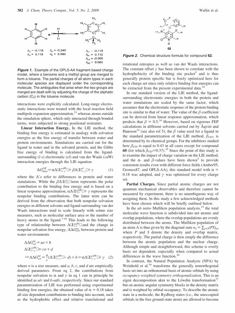
Figure 1. Example of the OPLS-AA fragment based chargemodel, where a benzene and a methyl group are merged toform a toluene. The partial charges of all atom types in eachmolecular species are displayed under the correspondingmolecule. The ambiguities that arise when the two groups aremerged are dealt with by adjusting the charge of the aliphaticcarbon (C2) in the toluene molecule.

Figure 2. Chemical structure formula for compound 62.

382 J. Chem. Theory Comput., Vol. 5, No. 2, 2009 Wallin et al.

weakly populated. The populations are then given by theeigenvalues in this decomposition.

In Atoms in Molecules theory (AIM) by Bader17,18 thenuclei of the molecule are attractors of the gradient densityfield, and an atom is consequently defined as being the basin

containing all the gradient trajectories terminating in itsnucleus. Integrating the density over this basin then givesthe atomic populations.

In lieu of populations, one may fit monopole charges tothe overall molecular electrostatic potential (ESP). Originally

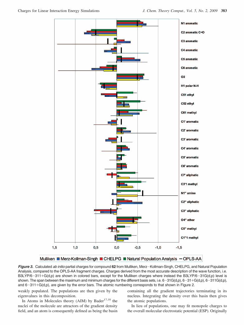
Figure 3. Calculated ab initio partial charges for compound 62 from Mulliken, Merz-Kollman-Singh, CHELPG, and Natural PopulationAnalysis, compared to the OPLS-AA fragment charges. Charges derived from the most accurate description of the wave function, i.e.B3LYP/6-311+G(d,p) are shown in colored bars, except for the Mulliken charges where instead the B3LYP/6-31G(d,p) level isshown. The span between the maximum and minimum charges for the different basis sets, i.e. 6-31G(d,p), 6-31+G(d,p), 6-311G(d,p),and 6-311+G(d,p), are given by the error bars. The atomic numbering corresponds to that shown in Figure 2.


introduced by Momany38 and Cox and Williams,39 thesemethods are based on the total density, which is a quantummechanical observable, and will thus provide experimentallyverifiable dipole and higher order multipole moments. In theMerz-Kollman-Singh (MK) variant, the potential is evalu-ated at points placed on the Connolly surface of themolecule40,41 onto which the charges are fitted in a least-squares manner, with a total integer charge constraint by themethod of Lagrange multipliers.20,42 The Charges fromElectrostatic Potentials scheme (CHELP) by Chirlian and

Francl43 is similar but with the points placed in concentric,symmetric, and nearly spherical shells about the atoms.Breneman and Wiberg19 suggested that the potential insteadbe evaluated in a grid of uniformly spaced points (CHELPG)to dampen its sensitivity toward conformational changes andis the variant that is used here.

Being evaluated at some distance (about 1.5-2.0 timesthe van der Waals-radii20), the charges of buried atoms (e.g.,sp3 carbons) have a tendency of being less important for thequality of the ESP fit than atoms closer to the molecular

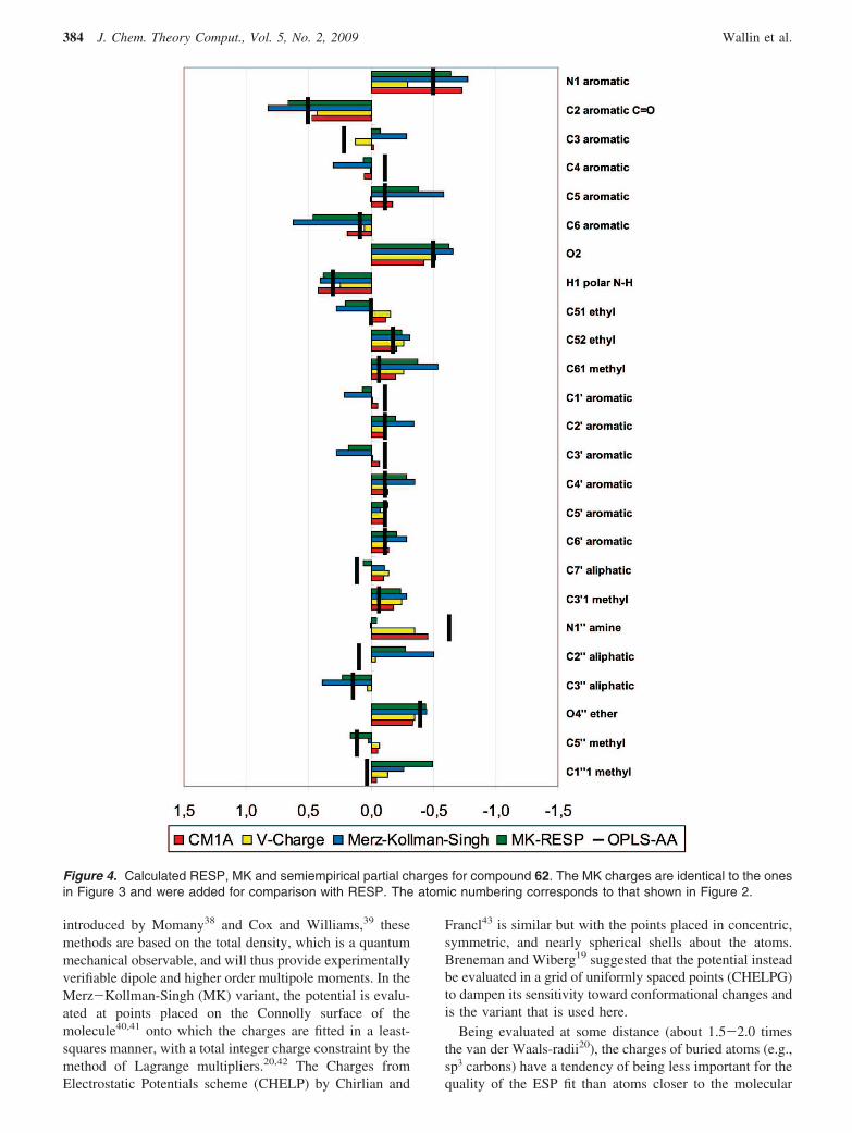
Figure 4. Calculated RESP, MK and semiempirical partial charges for compound 62. The MK charges are identical to the onesin Figure 3 and were added for comparison with RESP. The atomic numbering corresponds to that shown in Figure 2.


surface. For this reason, Bayly et al.44 suggested that thecharges on enveloped atoms be restrained with penaltyfunctions to dampen arbitrary fluctuations and to enforcesymmetry invariance, without deteriorating the overalldescription of the potential. Termed the Restrained Electro-static Potential (RESP) method this procedure is used in theAMBER force field definition.45,46

To reduce the computational effort, Cramer, Truhlar, andco-workers introduced the Charge Model 1A (CM1A) whichextracts Mulliken populations from NNDO Austin Model 1(AM1)47 semiempirical wave functions and subsequentlymaps them with a multilinear form to reproduce experimen-tally observed dipole moments.21 These charges have beensuccessfully used in solvation free energy calculations withthe OPLS-AA force field.13,48,49

Charges can also be inferred from the concept ofelectronegativity equalization where the atomic electrondensities are shifted to atoms with higher electronegativityupon bond formation, thus giving rise to partial charges.The subsequent increase in atomic radius corresponds toa lowering in electronegativity which continues untilequilibrium has been reached. Since total equalization willresult in e.g. all atoms in a molecule of the same sorthaving identical charges, Gasteiger and Marsili suggesteda partial equalization based on orbital electronegativites50

where the charge transfer is somewhat dampened.51 In theVcharge method, which is used here, Gilson et al. insteadadjusted the initial electronegativities based on the proper-ties of neighboring atoms, valence bond types, and a setof variables. The variables were parametrized on a set ofcompounds to reproduce the ab initio molecular ESP fromthe Hartree-Fock/6-31G(d) model chemistry.22 Thesemethods are computationally cheap and only require thechemical structure formula of the molecule.

Finally, charges have been derived in analogy with theOPLS-AA force field definition,29 where e.g. charges ofthe toluene molecule is found by maintaining the sym-metric benzene charges and then adjusting the methylcarbon charges to maintain the overall charge groupneutrality, as shown in Figure 1. Such charges arehenceforth referred to as the OPLS-AA fragment basedcharges. Although charge redistribution between fragmentsis not taken into account, these charges are most likely toremain balanced with the force field parameters of thewater model and the protein.

It may be noted that the Maestro software from Schrod-inger uses an automated fragment-based method with bondcharge increments52 to estimate junction atom charges.However, since this method requires optimized parametersfor it to be applicable to the OPLS-AA force field and theyare not publically available, this method will not be coveredin the present work.

The ab initio Mulliken, MK, CHELPG, and NPA chargeswere derived from density functional theory (DFT) wavefunctions at two levels of theory on structures optimized inthe gas phasesnamely B3LYP/6-31G(d,p)//B3LYP/6-31(d,p) and B3LYP/6-31G(d,p)//B3LYP/6-311+G(d,p).That is, using the Becke three parameter hybrid functional53

and the correlation functional of Lee, Yang, and Parr(B3LYP),54,55 together with Pople’s polarized split valenceand triple split contracted Gaussian basis sets, augmentedwith diffuse functions in the latter case.56 Furthermore, toget an estimate of the basis set dependence of the differentcharge schemes, wave functions were formed using theadditional basis sets 6-31+G(d,p) and 6-311G(d,p) forcompound 62, from which populations were derived withthe methods outlined above. Where nothing else is statedthe Gaussian 03 package57 was used for all ab initiocalculations.

The AIM calculations were performed with Bader’soriginal AIMPAC source code, using the PROMEGAalgorithm bundled in PROAIMV.58 However, since theoriginal settings only support molecules of at most 50 atoms,and the ligands considered herein are somewhat larger, theMCENT parameter was increased throughout the source codeto allow a maximum of 60 centers instead. The adoptednumerical integration parameters in the PROMEGA algo-rithm were 64 phi planes, 48 theta planes, and 96 radial pointsper integration ray within the Beta sphere. These settingsyielded an underestimation of the atomic basin populationsin the order of 3 to 6 · 10-4 e. To correct for these artificialpositive charges, the overall deviation from neutrality wasdivided equally across all basins and were subsequentlysubtracted. Although the absolute atomic net charges wereaffected by this correction, their relative charge differenceswere preserved.

To comply with the recommendations regarding the RESPcalculation scheme,44 Hartree-Fock densities with the6-31G(d) basis set were also formed from which the MKESP was extracted. RESP fitting of these charges wereperformed in two steps with the antechamber utility fromthe AmberTools distribution,59,60 using the ESP explicitoutput Gaussian internal option (IOp) 6/33)2. The ESPevaluation was set to 6 points per unit area using the IOp6/42)6.

CM1A charges were calculated with the Amsol software,61

and Gilson charges were obtained with Vcharge62 (VC/2004parameter set). As mentioned above, partial charges for theOPLS-AA charge set were assigned in analogy with the forcefield, except for the amine substituent of compound 68 whereRESP charges were used.

Charge Polarization. The propensity of a compound tobecome polarized when exposed to surroundings can begauged by calculating its static polarizability tensor r. This

Table 2. Static Average Polarizabilities and DipoleMoments in Gaseous and Aqueous Phase for theCompounds Studied Here, Using Two Levels of Theory

B3LYP/6-31G(d,p) B3LYP/6-311+G(d,p)

R [a03] µ(g) [D] µ(aq) [D] ∆µ µ(g) [D] µ(aq) [D] ∆µ

39 243 4.08 5.65 1.57 4.44 6.35 1.9140 259 3.84 5.26 1.42 4.03 5.65 1.6241 270 5.97 7.78 1.81 6.32 8.48 2.1646 244 4.02 5.86 1.84 4.36 6.64 2.2849 248 3.38 4.84 1.46 3.78 5.68 1.9052 273 4.23 5.69 1.46 4.68 6.54 1.8760 234 5.02 6.71 1.69 5.37 7.39 2.0262 233 4.81 6.71 1.89 5.29 7.65 2.3665 228 2.26 2.70 0.44 2.40 2.95 0.5468 294 5.56 8.40 2.84 5.76 9.07 3.31


tensor as well as higher order hyperpolarizabilities can beobtained from ab initio calculations where they are identifiedwith the analytic derivatives of the energy with respect tothe electric field at vanishing field strength.63 Furthermore,the average polarizability R, i.e. the mean of the tensordiagonal elements, is an invariant that can be inferred fromexperiments.64

Solvent induced polarization of the wave function canbe modeled using Self Consistent Reaction Field theory(SCRF) where the solute molecule is placed in a cavitysubmersed in an infinite continuous polarizable medium.To this end, a conductor-like extension of Tomasi’sapparent charge Polarizable Continuum Model65,66 (PCM),similar to the COSMO method by Klamt and Schuurman67,68

and termed Conductor-like PCM23,69 (CPCM), was usedhere.

Polarizabilities were extracted from frequency calculationsat the B3LYP/6-31G(d,p) level of theory. Where imaginaryfrequencies were detected, or the magnitude of the rotationallow frequencies surpassed ∼10 cm-1, the optimizations wereresubmitted with increased accuracy in the integration grid(see e.g. ref 70). The pruned UltraFine grid, with its 99 radialshells and 590 angular points, proved to be sufficient in allsuch cases.

CPCM polarization was implemented with the Gaussiankeyword, using the standard permittivity for water and the

default number of tesserae per sphere. Furthermore, theatomic radii of the United Atom Kohn-Sham topologicalmodel (UAKS) were used in all B3LYP calculations sincethese radii have been optimized with respect to DFT usingthe parameter free Perdew, Burke, and Ernzerhof functional(PBE0) at the 6-31G(d) level of theory.57 However, in theRESP Hartree-Fock calculations the default UA0 radii wereused.

Statistical Measures. The accuracy of the LIE bindingfree energy estimates with the different partial charge setswas measured with the coefficient of determination,denoted R2. Since the coefficient of determination com-pares the variance of the predictions with the total variancein the data, it is commonly used to measure the extent towhich the model explains the observed variance. For thesepurposes, however, it is enough to regard R2 as a simpleindication of the goodness-of-fit of the experimental datato the LIE regression line. Appropriately, the LIE param-eters that have been optimized here, e.g. the γ parameterin the LIE standard model, have been done so by least-squares regression, i.e. by minimizing the SSE with respectto experimental data.

Apart from gauging the extent of explained variance inthe model, it is also of special interest to measure the degreeof correspondence between the rankings, or the rank cor-

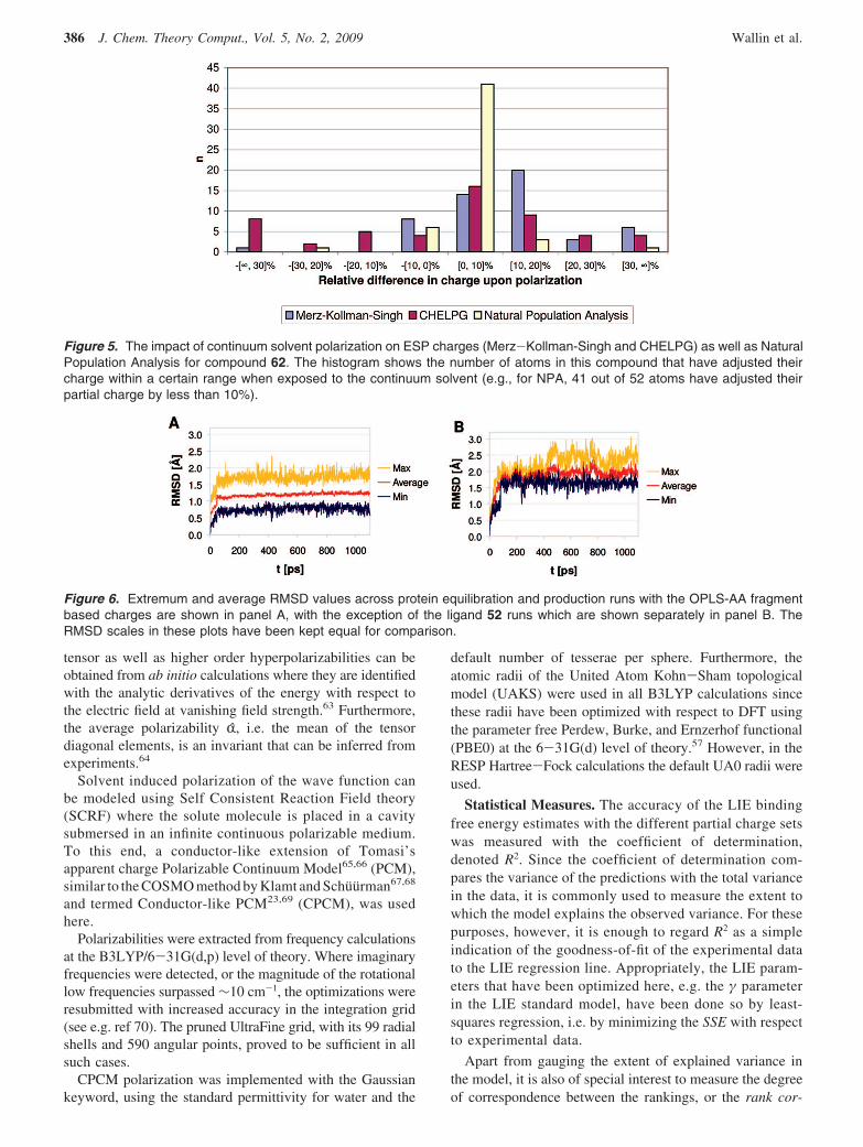
Figure 5. The impact of continuum solvent polarization on ESP charges (Merz-Kollman-Singh and CHELPG) as well as NaturalPopulation Analysis for compound 62. The histogram shows the number of atoms in this compound that have adjusted theircharge within a certain range when exposed to the continuum solvent (e.g., for NPA, 41 out of 52 atoms have adjusted theirpartial charge by less than 10%).

Figure 6. Extremum and average RMSD values across protein equilibration and production runs with the OPLS-AA fragmentbased charges are shown in panel A, with the exception of the ligand 52 runs which are shown separately in panel B. TheRMSD scales in these plots have been kept equal for comparison.


relation,71 between the observed and calculated binding freeenergies. A popular way of doing this in virtual high-throughput screening72 is by computing Spearman’s F value,given by

F) 1- 6S(d2)

n3 - n(3)

where n is the number of observations, and S(d2) denotesthe sum of squared differences between the experimental andcalculated ranking for each observation. Spearman’s F willthus be +1 if there is perfect agreement between the rankings,-1 if the sets are anticorrelated, and 0 if there is noagreement at all.

The error of the calculated binding free energy wasestimated with the standard error of the mean (SEM) takenwith respect to the ensemble averages in the protein startingfrom the three docking poses of each ligand. Given that thesample based estimation of the standard deviation is s andthe number of observations is nsin this case threesthe errorthen reads

Err[∆Gcalc])Rs[⟨Ulig-surr

Vdw ⟩prot

√n+ �

s[⟨Ulig-surrel ⟩prot

√n

Here it is assumed that the R and � parameters do notcontribute significantly to the uncertainty of the estimationwhen the LIE standard model is used.

Furthermore, leave-one-out cross-validated R2, commonlyreferred to as QLOO

2 , has been used as a quantitative methodto assess the predictive ability of the different LIE modelsand charge sets presented here. The definition of QLOO

2 issimilar to that of R2, namely

QLOO2 ) 1-

∑i

(∆Giobs -∆Gi

calc)2

∑i

(∆Giobs -∆G)2

(4)

The difference is that the binding energy of the ith ligandis estimated with a regression model on a data set wherethat particular compound was left out. If the model isdependent on the data points from which it was derived,this will have an impact on the QLOO

2 value. Followingcommon practice, charge sets that fall short of producinga QLOO

2 g 0.5 will be ruled out. Although externalvalidation is the most reliable method to assess predict-ability,73 internal validation is deemed quite adequate forthese purposes. However, Q2 can give a slight underes-timation of the true predictive error when applied to smalldata sets.74

Structural Stability and Convergence. The structuralstability of the ligand-protein complexes was estimated withthe root-mean-square deviation (RMSD), given as

RMSD([uF1...uF

n], [Vb1...Vbn]))�1n∑i)1

n

(uFi - VFi)2 (5)

In this case the RMSD was taken with respect to the heavyatom position vectors of the ligand structures, which werekept unfitted since the ligands are more or less held inposition by the protein. By this choice rotation and translationare expected to have a significant impact on the computedvalues.

Before considering the impact of varying charges, thestructural stability of the OPLS-AA fragment based chargeruns was measured with respect to the starting structures,[xb(0)1...n]i

j, of ligand i and pose j, hence RMSD(t)-([xb(0)1...n]i

j,[xb(t)1...n]ij). Then the charge model (CM) stability

was measured by forming production phase averagestructures, ⟨CM⟩ , and computing their RMSD with respectto OPLS-AA. That is, for the nth charge model this readsRMSD(⟨OPLSAA⟩ i

j,⟨CMn⟩ ij), for ligand i and pose j. The

former comparison is meant to gauge the overall stabilityof the system per se, whereas the latter reflects the impactof charge variation on the structures.

Since the RMSD values were extracted from 690 MDruns, a few operations were defined to simplify thepresentation of this data. For the initial OPLS-AA stability,extremum and average RMSD values across all ligandsand poses as a function of time are presented. Whencomparing charge models with the OPLS-AA averagestructures, the RMSD values were summed over the poses,that is ∑jRMSD(⟨OPLSAA⟩ i

j,⟨CMn⟩ ij).

Results and Discussion

To begin with, the actual differences in charge between themodels will be investigated for a representative compoundfrom the ligand set. Then the calculated polarizabilites andtheir impact on the calculated effective dipole moments, i.e.when subjected to implicit solvent, are presented. After this,the charge sets are culled, first with respect to the precision,as given by the convergence of the MD ensemble averages,

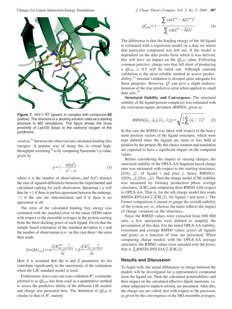
Figure 7. HIV-1 RT (green) in complex with compound 62(yellow). The structure is a docking solution used as a startingstructure in MD simulations. The figure shows the closeproximity of Lys103 (blue) to the carbonyl oxygen of thepyridinone.


and then on the accuracy in their binding free energyestimates. Finally, the reliability of these results is examinedthrough statistical internal validation.

Comparing Charges. To get an overview of how partialcharges actually differ between the charge models, ligand62 (see Figure 2) was chosen as a representative compound,and the derived ab initio charges of its first row atoms andthe polar N-H hydrogen are displayed in Figure 3. To beginwith, charge dependence on level of the model chemistrywas gauged by performing DFT calculations with a rangeof basis sets, namely 6-31G(d,p) and 6-311G(d,p) with andwithout the addition of diffuse functions. Charges derivedfrom the highest level of theory are displayed in Figure 3,with the exception of the Mulliken charges where insteadthe low level is shown, as well as the span between thecharge assignments which is shown in the error bars. Asexpected, the sensitivity toward the choice of basis set ismost apparent for the Mulliken charges, where for instancethe C3 atom of the pyridinone ring (defined in Figure 2)ranges from being neutral to highly negative (∼-1.5 e) whenadding diffuse functions. This is presumably due to theconsiderable overlap populations. In contrast, the NPA andthe ESP charges are significantly more stable in this respect.

Apart from basis set impact, charge assignment from thedifferent methods is seen to vary throughout, which is onlynatural considering that the atomic partial charges are notquantum mechanical observables and thus cannot be directlymeasured by experiment. Any charge assignment willtherefore be more or less arbitrary. In particular, substituentatoms that link functional groups together seem to be difficultto assign by any method, e.g. C51, C7′, the tertiary N1′′ ,and its neighbors. However, there are a few cases where thereis a remarkable agreement between all the methods, such asthe ether O4′′ and the pyridinone polar H1 atoms. Also, it isreassuring to see an overall similarity between the ESPcharges from the MK and CHELPG schemes. Moreover,charge redistribution seems to be causing the most pro-nounced overall difference between the OPLS-AA fragmentbased charges and the ab initio sets. For instance, thearomatic C1′-C6′ atoms are seen to be in fair agreementexcept where the aliphatic substituents are bound, i.e. C1′and C3′. This can also be seen in the pyridinone ring C3and C4 atoms.

In order to compare the CM1A and Vcharge sets withOPLS-AA and ab initio charges, they are plotted along withthe MK ESP charges in Figure 4. Also included in this plotare the RESP fitted charges, which were extracted from theHartree-Fock ESP using the 6-31G(d) basis set, rather thanthe high level DFT wave functions. In spite of thesedifferences, the RESP charges are seen to be very similar tothe MK set.

The overall picture that emerges in this figure is just aboutthe same as in Figure 3. The charge redistribution that isdisregarded in the fragment based method is indeed capturedby the emipirical models, where CM1A seems to lie closestto the OPLS-AA charges. The overall RMSD between theCM1A and Vcharge set is 0.09 e, the largest difference beingthe pyridinone nitrogen where CM1A is substantially morepolarized. There are a few cases where they deviate from

OPLS-AA, e.g. the amine N1′′ and C′7, but the impressionis that they are more consistent with the force field than theMK and RESP charges.

Polarizability and Solvent Effects. The charges thatwere discussed in the previous section were all derivedin Vacuo. However, drug binding and hydration pertainto polar surroundings that can have a significant impacton the overall electrostatic properties of the compounddue to polarization. For this reason, it seems useful toestimate the importance of charge polarization for thesecompounds, either by including an environment in thecalculation or by studying their intrinsic static averagepolarizability in vacuum. In the latter case, a significantpolarizability indicates that the charges may vary as theligand is subjected to different surroundings. The polar-izability of the wave function was thus calculated andcompared with the change in dipole moment as thecompounds are subjected to the implicit solvation model.As expected, the presence of aromatic groups results insignificant polarizabilities ranging from about 200 to 300a0

3 (see Table 2), which may be compared with thepolarizability of, for instance, water which is 10.13 a0

3

(∆calc-exp ) -4.78 a03), methane 16.52 (∆calc-exp ) -3.84)

a03, and ammonia 14.19 (∆calc-exp ) -5.61) a0

3, with themodel chemistry used here (values from ref 75), wherea0 is the Bohr radius. This is in turn reflected in thesignificant increase of the dipole moment, by up to 3 D,when exposed to the implicit solvent model (see Table2).

It seems rather clear that the impact of the solvent on thetotal charge distribution, as represented by the dipolemoments, should also appear as changes in the partialcharges. Indeed, plotting the distributions of the relativechanges in atomic charge when compound 62 is exposed tosolvent shows that they change by 10% or more due topolarization when ESP methods are used (see Figure 5). Incontrast, polarization does not seem to affect NPA chargesas much, where only four atoms change by more than 10%.This difference can perhaps be understood by consideringthat the ESP is directly based on the overall chargedistribution. The increase in the dipole moments and itsimpact on the partial charges substantiates the typical choiceof using charges derived from the HF/6-31G(d) level oftheory,44 which usually overestimates the dipole moment ofthe molecule to an extent that roughly corresponds to itseffective value in aqueous solution. However, it should benoted that this effect does not seem to be as pronounced forthe B3LYP model chemistries that are used here.75 Chargepolarization is also the motivation behind linear scaling ofcharges present in the OPLS/CM1A force field,48 i.e. wherethe CM1A charges are multiplied by a factor of 1.14 toenhance solvation free energy estimates. This linear scalinghas also been included in this study.

Stability and Convergence. As outlined in the Methodssection, the binding free energy estimates in the LIE methodare calculated from ensemble averages of the ligand-surrounding interaction energies, which are extracted frommolecular dynamics trajectories. Every ligand is simulatedfrom three different docking poses for every charge set, and


since these poses were selected from the same binding modethe resulting energies are given as the mean from the threesimulations. It should be noted that in cases where posescannot interchange during the course of the simulation itwould be hard to justify that they are in thermal equilibriumand so the averages would have to be Boltzmann weighted.

It is important that the MD runs have converged structur-ally and energetically, both within one and the same run andbetween simulations with different docking poses, since thiswill determine the precision in the binding free energyestimates. Structurally, the simulations are stable with lowRMSD of the ligands and only minor fluctuations in theprotein. Specifically, in the reference OPLS-AA chargesimulations the maximum unfitted RMSD among the teninhibitors and their three poses is largest for compound 52,namely 3.1 Å, whereas it does not exceed 2.3 Å for the otherligands. However, the largest contribution to this value occursduring equilibration, after which the ligands have settled intoa position on average differing by 1.9 Å for compound 52and 1.2 Å for the rest (Figure 6). After this initial displace-ment the fluctuations about their equilibrated positions arequite small. Such small variations are expected since theinhibitors are rigid and bind to a well-defined allostericpocket. The main structural fluctuation, occurring only in afew cases, is found in the side chain of Lys103, which islocated close to the carbonyl group of the pyridinone ringin the docked starting position (Figure 7) as well as in the

crystal structure.26 In cases where this lysine leaves thecarboxyl group and starts to interact with the solvent, theelectrostatic ligand-surrounding energies are substantiallydecreased, which results in an increase in the predictedbinding free energy.

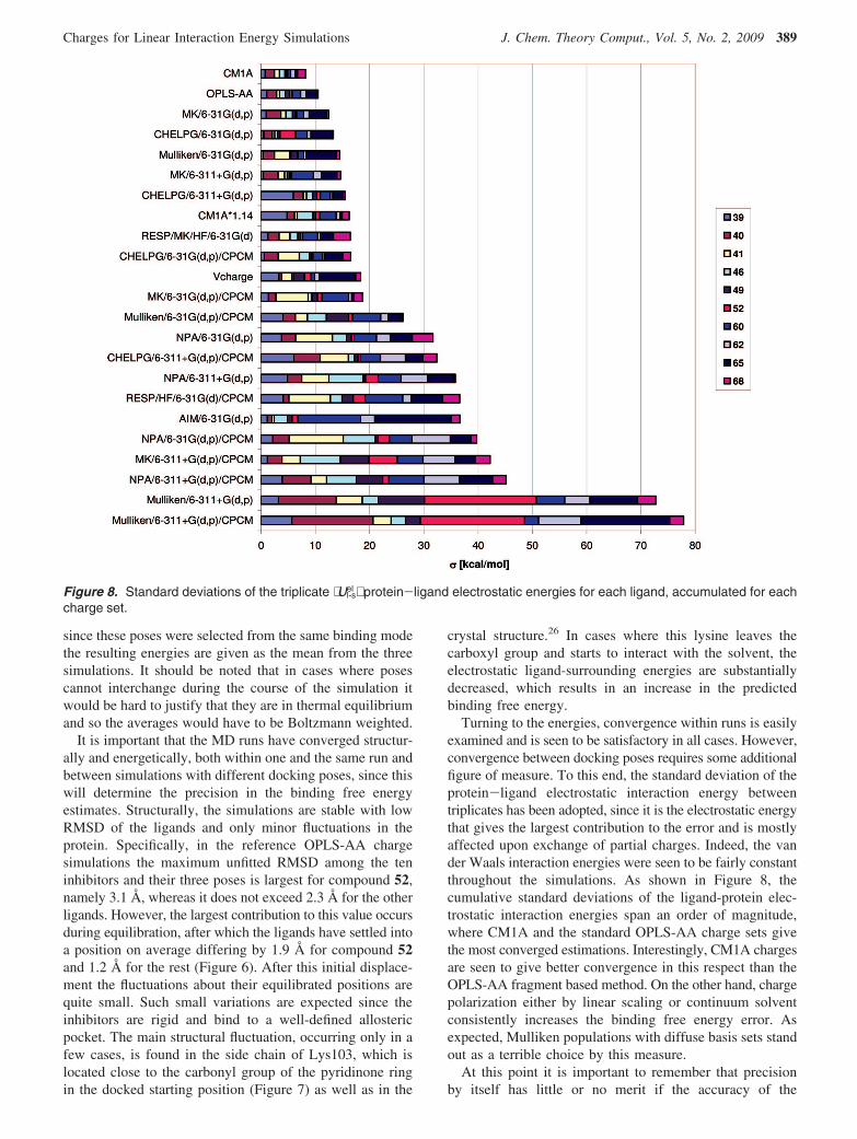
Turning to the energies, convergence within runs is easilyexamined and is seen to be satisfactory in all cases. However,convergence between docking poses requires some additionalfigure of measure. To this end, the standard deviation of theprotein-ligand electrostatic interaction energy betweentriplicates has been adopted, since it is the electrostatic energythat gives the largest contribution to the error and is mostlyaffected upon exchange of partial charges. Indeed, the vander Waals interaction energies were seen to be fairly constantthroughout the simulations. As shown in Figure 8, thecumulative standard deviations of the ligand-protein elec-trostatic interaction energies span an order of magnitude,where CM1A and the standard OPLS-AA charge sets givethe most converged estimations. Interestingly, CM1A chargesare seen to give better convergence in this respect than theOPLS-AA fragment based method. On the other hand, chargepolarization either by linear scaling or continuum solventconsistently increases the binding free energy error. Asexpected, Mulliken populations with diffuse basis sets standout as a terrible choice by this measure.

At this point it is important to remember that precisionby itself has little or no merit if the accuracy of the

Figure 8. Standard deviations of the triplicate ⟨Ul-sel ⟩ protein-ligand electrostatic energies for each ligand, accumulated for each

charge set.


predictions is disregarded. For instance, with the presentfigure of measure one would obtain a very high precisionby neutralizing all the charges but at a cost of severelyreducing the accuracy of the predictions. Conversely, if thereare models here that give highly accurate predictions but witha very low precision, they will be hard to distinguish fromrandom noisesespecially on such a limited number ofobservations. For this reason, it is argued that both precisionand accuracy are of moment here, and charge sets with anaccumulated standard deviation in ligand-surrounding elec-trostatic energies that exceeds 20 kcal/mol are thereforediscarded henceforth.

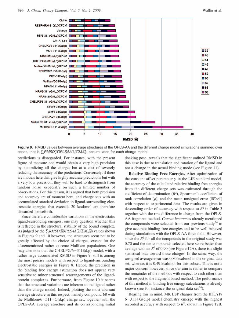
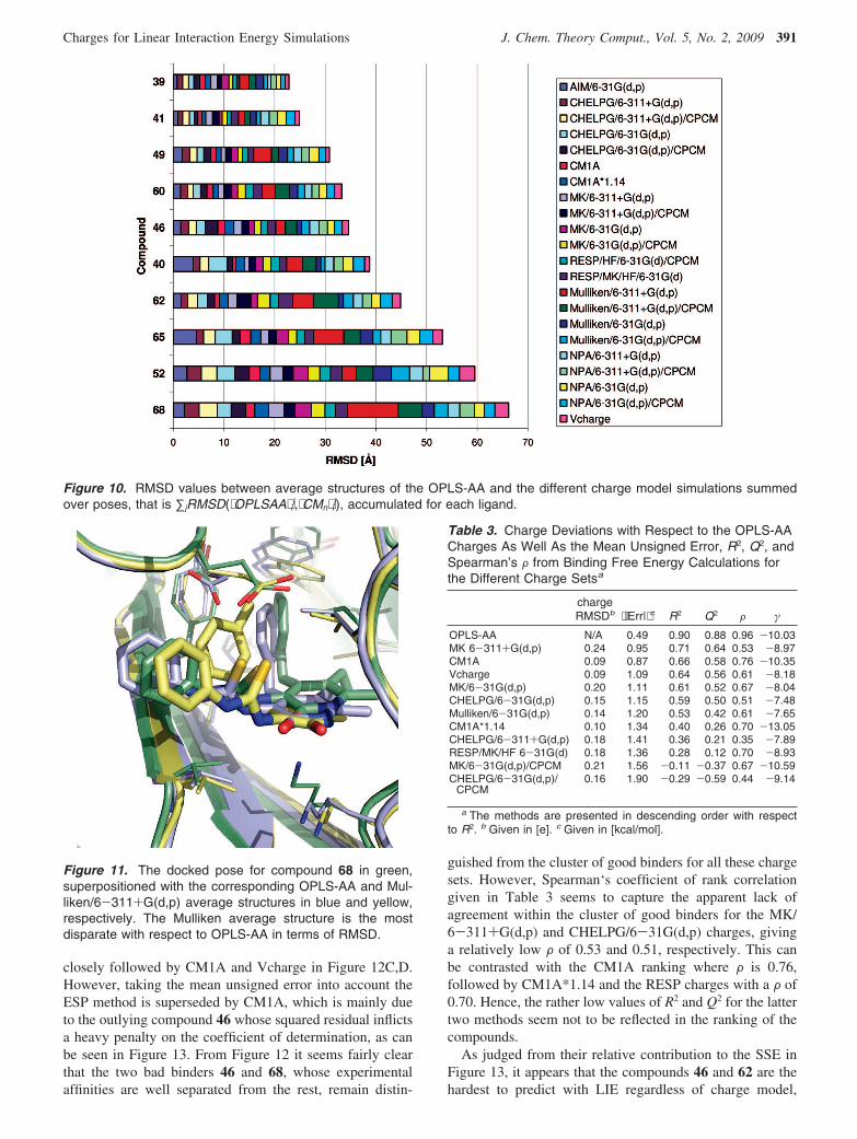
Since there are considerable variations in the electrostaticligand-surronding energies, one may question whether thisis reflected in the structural stability of the bound complex.As judged by the ∑jRMSD(⟨OPLSAA⟩ i

j,⟨CMn⟩ ij) values shown

in Figures 9 and 10 however, the structures seem not to begreatly affected by the choice of charges, except for theaforementioned rather extreme Mulliken populations. Onemay also note that the CHELPG/6-31G(d,p) model, with arather large accumulated RMSD in Figure 9, still is amongthe most precise models with respect to ligand-surroundingelectrostatic energies in Figure 8. Hence, the precision inthe binding free energy estimation does not appear verysensitive to minor structural rearrangements of the ligand-protein complexes. Furthermore, from Figure 10 it seemsthat the structural variations are inherent to the ligand ratherthan the charge model. Indeed, plotting the most aberrantaverage structure in this respect, namely compound 68 withthe Mulliken/6-311+G(d,p) charge set, together with theOPLS-AA average structure and its corresponding initial

docking pose, reveals that the significant unfitted RMSD inthis case is due to translation and rotation of the ligand andnot a change in the actual binding mode (see Figure 11).

Relative Binding Free Energies. After optimization ofthe constant offset parameter γ in the LIE standard model,the accuracy of the calculated relative binding free energiesfrom the different charge sets was estimated through thecoefficient of determination (R2), Spearman’s coefficient ofrank correlation (F), and the mean unsigned error (⟨ |Err|⟩)with respect to experimental data. The results are given indescending order of accuracy with respect to R2 in Table 3together with the rms difference in charge from the OPLS-AA fragment method. CaVeat lectorsas already mentionedthe compounds were selected from our previous study24 togive accurate binding free energies and to be well behavedduring simulations with the OPLS-AA force field. However,since the R2 for all the compounds in the original study was0.70 and the ten compounds selected here score better thanaverage with an R2 of 0.90 (see Figure 12A), there is a slightstatistical bias toward these charges. In the same way, theunsigned average error was 0.80 kcal/mol in the original dataset, whereas it is 0.49 kcal/mol for this subset. This is not amajor concern however, since our aim is rather to comparethe remainder of the methods with respect to each other thanwith respect to the fragment based method. The performanceof this method in binding free energy calculations is alreadyknown (see for instance the original data set24).

Bearing this in mind, MK ESP charges from the B3LYP/6-311+G(d,p) model chemistry emerge with the highestrecorded accuracy with respect to R2, shown in Figure 12B,

Figure 9. RMSD values between average structures of the OPLS-AA and the different charge model simulations summed overposes, that is ∑jRMSD(⟨OPLSAA⟩ i

j,⟨CMn⟩ ij), accumulated for each charge model.


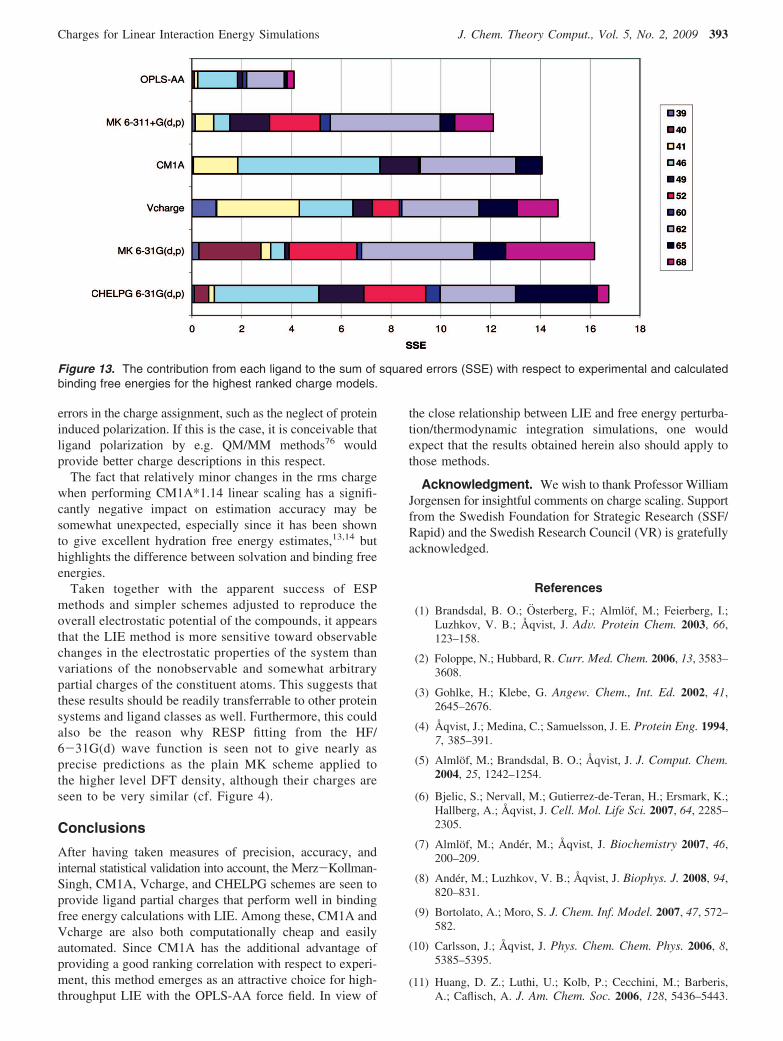
closely followed by CM1A and Vcharge in Figure 12C,D.However, taking the mean unsigned error into account theESP method is superseded by CM1A, which is mainly dueto the outlying compound 46 whose squared residual inflictsa heavy penalty on the coefficient of determination, as canbe seen in Figure 13. From Figure 12 it seems fairly clearthat the two bad binders 46 and 68, whose experimentalaffinities are well separated from the rest, remain distin-

guished from the cluster of good binders for all these chargesets. However, Spearman‘s coefficient of rank correlationgiven in Table 3 seems to capture the apparent lack ofagreement within the cluster of good binders for the MK/6-311+G(d,p) and CHELPG/6-31G(d,p) charges, givinga relatively low F of 0.53 and 0.51, respectively. This canbe contrasted with the CM1A ranking where F is 0.76,followed by CM1A*1.14 and the RESP charges with a F of0.70. Hence, the rather low values of R2 and Q2 for the lattertwo methods seem not to be reflected in the ranking of thecompounds.

As judged from their relative contribution to the SSE inFigure 13, it appears that the compounds 46 and 62 are thehardest to predict with LIE regardless of charge model,

Figure 10. RMSD values between average structures of the OPLS-AA and the different charge model simulations summedover poses, that is ∑jRMSD(⟨OPLSAA⟩ i

j,⟨CMn⟩ ij), accumulated for each ligand.

Figure 11. The docked pose for compound 68 in green,superpositioned with the corresponding OPLS-AA and Mul-liken/6-311+G(d,p) average structures in blue and yellow,respectively. The Mulliken average structure is the mostdisparate with respect to OPLS-AA in terms of RMSD.

Table 3. Charge Deviations with Respect to the OPLS-AACharges As Well As the Mean Unsigned Error, R2, Q2, andSpearman’s F from Binding Free Energy Calculations forthe Different Charge Setsa

chargeRMSDb ⟨ |Err|⟩c R2 Q2 F γ

OPLS-AA N/A 0.49 0.90 0.88 0.96 -10.03MK 6-311+G(d,p) 0.24 0.95 0.71 0.64 0.53 -8.97CM1A 0.09 0.87 0.66 0.58 0.76 -10.35Vcharge 0.09 1.09 0.64 0.56 0.61 -8.18MK/6-31G(d,p) 0.20 1.11 0.61 0.52 0.67 -8.04CHELPG/6-31G(d,p) 0.15 1.15 0.59 0.50 0.51 -7.48Mulliken/6-31G(d,p) 0.14 1.20 0.53 0.42 0.61 -7.65CM1A*1.14 0.10 1.34 0.40 0.26 0.70 -13.05CHELPG/6-311+G(d,p) 0.18 1.41 0.36 0.21 0.35 -7.89RESP/MK/HF 6-31G(d) 0.18 1.36 0.28 0.12 0.70 -8.93MK/6-31G(d,p)/CPCM 0.21 1.56 -0.11 -0.37 0.67 -10.59CHELPG/6-31G(d,p)/

CPCM0.16 1.90 -0.29 -0.59 0.44 -9.14

a The methods are presented in descending order with respectto R2. b Given in [e]. c Given in [kcal/mol].


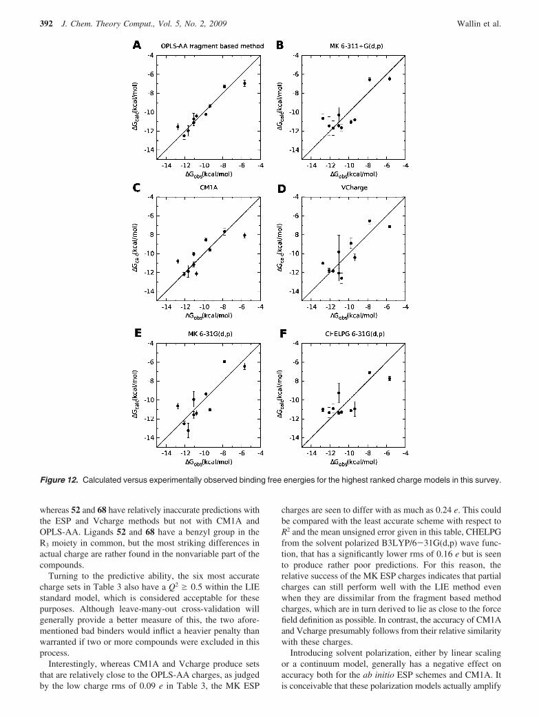
whereas 52 and 68 have relatively inaccurate predictions withthe ESP and Vcharge methods but not with CM1A andOPLS-AA. Ligands 52 and 68 have a benzyl group in theR3 moiety in common, but the most striking differences inactual charge are rather found in the nonvariable part of thecompounds.

Turning to the predictive ability, the six most accuratecharge sets in Table 3 also have a Q2 g 0.5 within the LIEstandard model, which is considered acceptable for thesepurposes. Although leave-many-out cross-validation willgenerally provide a better measure of this, the two afore-mentioned bad binders would inflict a heavier penalty thanwarranted if two or more compounds were excluded in thisprocess.

Interestingly, whereas CM1A and Vcharge produce setsthat are relatively close to the OPLS-AA charges, as judgedby the low charge rms of 0.09 e in Table 3, the MK ESP

charges are seen to differ with as much as 0.24 e. This couldbe compared with the least accurate scheme with respect toR2 and the mean unsigned error given in this table, CHELPGfrom the solvent polarized B3LYP/6-31G(d,p) wave func-tion, that has a significantly lower rms of 0.16 e but is seento produce rather poor predictions. For this reason, therelative success of the MK ESP charges indicates that partialcharges can still perform well with the LIE method evenwhen they are dissimilar from the fragment based methodcharges, which are in turn derived to lie as close to the forcefield definition as possible. In contrast, the accuracy of CM1Aand Vcharge presumably follows from their relative similaritywith these charges.

Introducing solvent polarization, either by linear scalingor a continuum model, generally has a negative effect onaccuracy both for the ab initio ESP schemes and CM1A. Itis conceivable that these polarization models actually amplify

Figure 12. Calculated versus experimentally observed binding free energies for the highest ranked charge models in this survey.


errors in the charge assignment, such as the neglect of proteininduced polarization. If this is the case, it is conceivable thatligand polarization by e.g. QM/MM methods76 wouldprovide better charge descriptions in this respect.

The fact that relatively minor changes in the rms chargewhen performing CM1A*1.14 linear scaling has a signifi-cantly negative impact on estimation accuracy may besomewhat unexpected, especially since it has been shownto give excellent hydration free energy estimates,13,14 buthighlights the difference between solvation and binding freeenergies.

Taken together with the apparent success of ESPmethods and simpler schemes adjusted to reproduce theoverall electrostatic potential of the compounds, it appearsthat the LIE method is more sensitive toward observablechanges in the electrostatic properties of the system thanvariations of the nonobservable and somewhat arbitrarypartial charges of the constituent atoms. This suggests thatthese results should be readily transferrable to other proteinsystems and ligand classes as well. Furthermore, this couldalso be the reason why RESP fitting from the HF/6-31G(d) wave function is seen not to give nearly asprecise predictions as the plain MK scheme applied tothe higher level DFT density, although their charges areseen to be very similar (cf. Figure 4).

Conclusions

After having taken measures of precision, accuracy, andinternal statistical validation into account, the Merz-Kollman-Singh, CM1A, Vcharge, and CHELPG schemes are seen toprovide ligand partial charges that perform well in bindingfree energy calculations with LIE. Among these, CM1A andVcharge are also both computationally cheap and easilyautomated. Since CM1A has the additional advantage ofproviding a good ranking correlation with respect to experi-ment, this method emerges as an attractive choice for high-throughput LIE with the OPLS-AA force field. In view of

the close relationship between LIE and free energy perturba-tion/thermodynamic integration simulations, one wouldexpect that the results obtained herein also should apply tothose methods.

Acknowledgment. We wish to thank Professor WilliamJorgensen for insightful comments on charge scaling. Supportfrom the Swedish Foundation for Strategic Research (SSF/Rapid) and the Swedish Research Council (VR) is gratefullyacknowledged.

References

(1) Brandsdal, B. O.; Osterberg, F.; Almlof, M.; Feierberg, I.;Luzhkov, V. B.; Åqvist, J. AdV. Protein Chem. 2003, 66,123–158.

(2) Foloppe, N.; Hubbard, R. Curr. Med. Chem. 2006, 13, 3583–3608.

(3) Gohlke, H.; Klebe, G. Angew. Chem., Int. Ed. 2002, 41,2645–2676.

(4) Åqvist, J.; Medina, C.; Samuelsson, J. E. Protein Eng. 1994,7, 385–391.

(5) Almlof, M.; Brandsdal, B. O.; Åqvist, J. J. Comput. Chem.2004, 25, 1242–1254.

(6) Bjelic, S.; Nervall, M.; Gutierrez-de-Teran, H.; Ersmark, K.;Hallberg, A.; Åqvist, J. Cell. Mol. Life Sci. 2007, 64, 2285–2305.

(7) Almlof, M.; Ander, M.; Åqvist, J. Biochemistry 2007, 46,200–209.

(8) Andér, M.; Luzhkov, V. B.; Åqvist, J. Biophys. J. 2008, 94,820–831.

(9) Bortolato, A.; Moro, S. J. Chem. Inf. Model. 2007, 47, 572–582.

(10) Carlsson, J.; Åqvist, J. Phys. Chem. Chem. Phys. 2006, 8,5385–5395.

(11) Huang, D. Z.; Luthi, U.; Kolb, P.; Cecchini, M.; Barberis,A.; Caflisch, A. J. Am. Chem. Soc. 2006, 128, 5436–5443.

Figure 13. The contribution from each ligand to the sum of squared errors (SSE) with respect to experimental and calculatedbinding free energies for the highest ranked charge models.


(12) Kolb, P.; Huang, D.; Dey, F.; Caflisch, A. J. Med. Chem.2008, 51, 1179–1188.

(13) Udier-Blagovic, M.; De Tirado, P. M.; Pearlman, S. A.;Jorgensen, W. L. J. Comput. Chem. 2004, 25, 1322–1332.

(14) Mobley, D. L.; Dumont, E.; Chodera, J. D.; Dill, K. A. J.Phys. Chem. B 2007, 111, 2242–2254.

(15) Mulliken, R. S. J. Chem. Phys. 1955, 23, 1833–1840.

(16) Reed, A. E.; Weinstock, R. B.; Weinhold, F. J. Chem. Phys.1985, 83, 735–746.

(17) Bieglerkonig, F. W.; Bader, R. F. W.; Tang, T. H. J. Comput.Chem. 1982, 3, 317–328.

(18) Bieglerkonig, F. W.; Nguyendang, T. T.; Tal, Y.; Bader,R. F. W.; Duke, A. J. J. Phys. B: At., Mol. Opt. Phys. 1981,14, 2739–2751.

(19) Breneman, C. M.; Wiberg, K. B. J. Comput. Chem. 1990,11, 361–373.

(20) Singh, U. C.; Kollman, P. A. J. Comput. Chem. 1984, 5,129–145.

(21) Storer, J. W.; Giesen, D. J.; Cramer, C. J.; Truhlar, D. G.J. Comput.-Aided Mol. Des. 1995, 9, 87–110.

(22) Gilson, M. K.; Gilson, H. S. R.; Potter, M. J. J. Chem. Inf.Comput. Sci. 2003, 43, 1982–1997.

(23) Barone, V.; Cossi, M. J. Phys. Chem. A 1998, 102, 1995–2001.

(24) Carlsson, J.; Boukharta, L.; Åqvist, J. J. Med. Chem. 2008,51, 2648–2656.

(25) Benjahad, A.; Croisy, M.; Monneret, C.; Bisagni, E.; Mabire,D.; Coupa, S.; Poncelet, A.; Csoka, I.; Guillemont, J.; Meyer,C.; Andries, K.; Pauwels, R.; de Bethune, M. P.; Himmel,D. M.; Das, K.; Arnold, E.; Nguyen, C. H.; Grierson, D. S.J. Med. Chem. 2005, 48, 1948–1964.

(26) Himmel, D. M.; Das, K.; Clark, A. D.; Hughes, S. H.;Benjahad, A.; Oumouch, S.; Guillemont, J.; Coupa, S.;Poncelet, A.; Csoka, I.; Meyer, C.; Andries, K.; Nguyen, C. H.;Grierson, D. S.; Arnold, E. J. Med. Chem. 2005, 48, 7582.

(27) Jones, G.; Willett, P.; Glen, R. C.; Leach, A. R.; Taylor, R.J. Mol. Biol. 1997, 267, 727–748.

(28) Marelius, J.; Kolmodin, K.; Feierberg, I.; Åqvist, J. J. Mol.Graphics Modell. 1998, 16, 213–225.

(29) Jorgensen, W. L.; Maxwell, D. S.; TiradoRives, J. J. Am.Chem. Soc. 1996, 118, 11225–11236.

(30) Jorgensen, W.; Chandrasekhar, J.; Madura, J.; Rw, I.; Klein,M. J. Chem. Phys. 1983, 79, 926–935.

(31) Ryckaert, J. P.; Ciccotti, G.; Berendsen, H. J. C. J. Comput.Phys. 1977, 23, 327–341.

(32) King, G.; Warshel, A. J. Chem. Phys. 1989, 91, 3647–3661.

(33) Lee, F. S.; Warshel, A. J. Chem. Phys. 1992, 97, 3100–3107.

(34) Åqvist, J.; Hansson, T. J. Phys. Chem. 1996, 100, 9512–9521.

(35) Hansson, T.; Marelius, J.; Åqvist, J. J. Comput.-Aided Mol.Des. 1998, 12, 27–35.

(36) Luthi, H. P.; Ammeter, J. H.; Almlof, J.; Faegri, K. J. Chem.Phys. 1982, 77, 2002–2009.

(37) Lowdin, P. O. J. Chem. Phys. 1950, 18, 365–375.

(38) Momany, F. A. J. Phys. Chem. 1978, 82, 592–601.

(39) Cox, S. R.; Williams, D. E. J. Comput. Chem. 1981, 2, 304–323.

(40) Connolly, M. L. J. Appl. Crystallogr. 1983, 16, 548–558.

(41) Connolly, M. L. Science 1983, 221, 709–713.

(42) Besler, B. H.; Merz, K. M.; Kollman, P. A. J. Comput. Chem.1990, 11, 431–439.

(43) Chirlian, L. E.; Francl, M. M. J. Comput. Chem. 1987, 8,894–905.

(44) Bayly, C. I.; Cieplak, P.; Cornell, W. D.; Kollman, P. A. J.Phys. Chem. 1993, 97, 10269–10280.

(45) Cornell, W. D.; Cieplak, P.; Bayly, C. I.; Gould, I. R.; Merz,K. M.; Ferguson, D. M.; Spellmeyer, D. C.; Fox, T.; Caldwell,J. W.; Kollman, P. A. J. Am. Chem. Soc. 1996, 118, 2309–2309.

(46) Wang, J. M.; Cieplak, P.; Kollman, P. A. J. Comput. Chem.2000, 21, 1049–1074.

(47) Dewar, M. J. S.; Zoebisch, E. G.; Healy, E. F.; Stewart, J. J. P.J. Am. Chem. Soc. 1985, 107, 3902–3909.

(48) Jorgensen, W. L.; Tirado-Rives, J. Proc. Natl. Acad. Sci.U.S.A. 2005, 102, 6665–6670.

(49) Kaminski, G. A.; Jorgensen, W. L. J. Phys. Chem. B 1998,102, 1787–1796.

(50) Hinze, J.; Whitehead, M. A.; Jaffe, H. H. J. Am. Chem. Soc.1963, 85, 148.

(51) Gasteiger, J.; Marsili, M. Tetrahedron 1980, 36, 3219–3228.

(52) Halgren, T. A. J. Comput. Chem. 1996, 17, 616–641.

(53) Becke, A. D. J. Chem. Phys. 1993, 98, 5648–5652.

(54) Lee, C. T.; Yang, W. T.; Parr, R. G. Phys. ReV. B 1988, 37,785–789.

(55) Miehlich, B.; Savin, A.; Stoll, H.; Preuss, H. Chem. Phys.Lett. 1989, 157, 200–206.

(56) Frisch, M. J.; Pople, J. A.; Binkley, J. S. J. Chem. Phys. 1984,80, 3265–3269.

(57) Gaussian 03, reVision C.02; Gaussian Inc.: Wallingford, CT,2004.

(58) AIMPAC, Version 94; Department of Chemistry, McMasterUniversity: Hamilton, Ontario, Canada, 1994.

(59) AmberTools, 1.2; University of California: San Fransisco, CA,2008.

(60) Case, D. A.; Cheatham, T. E., III; Darden, T.; Gohlke, H.;Luo, R.; Merz, K. M. J.; Onufriev, A.; Simmerling, C.; Wang,B.; Woods, R. J. J. Comput. Chem. 2005, 26, 1668.

(61) AMSOL, Version 7.0; University of Minnesota: Minneapolis,MN, 2003.

(62) Vcharge, 1.0; VeraChem LLC: Germantown, MD, 2004.

(63) Pugh, D. Electric multipoles, polarizabilities and hyperpolar-izabilities In Chemical Modelling: Applications and Theory;Hinchliffe, A., Ed.; RSC: Cambridge, U.K., 2000; Vol. 1, pp1-37.

(64) HerzbergG. Vibrational infrared and and Raman spectra.In Infrared and Raman spectra of polyatomic molecules;1st ed.; Van Nostrand: New York, NY 1945; pp 239-269.

(65) Miertus, S.; Scrocco, E.; Tomasi, J. Chem. Phys. 1981, 55,117–129.

(66) Miertus, S.; Tomasi, J. Chem. Phys. 1982, 65, 239–245.


(67) Klamt, A.; Schuurmann, G. J. Chem. Soc., Perkin Trans. 21993, 799, 805.

(68) Klamt, A. J. Phys. Chem. 1995, 99, 2224–2235.

(69) Cossi, M.; Rega, N.; Scalmani, G.; Barone, V. J. Comput.Chem. 2003, 24, 669–681.

(70) Ochterski, J. Vibrational analysis in Gaussian, 1999. Gaussianwhite papers. http://www.gaussian.com/g_whitepap/vib.htm(accessed Aug 11, 2007).

(71) Kendall, M. G. The measurement of rank correlation. In RankCorrelation Methods; 1st ed.; Charles Griffin and Co.:London, U.K., 1948; pp 8-10.

(72) Seifert, M. H. J.; Kraus, J.; Kramer, B. Curr. Opin. DrugDiscoVery DeV. 2007, 10, 298–307.

(73) Golbraikh, A.; Tropsha, A. J. Mol. Graphics Modell. 2002,20, 269–276.

(74) Martens, H. A.; Dardenne, P. Chemom. Intell. Lab. Syst.1998, 44, 99–121.

(75) Johnson, R. D., IIINIST Computational Chemistry Comparisonand Benchmark Database, 2005. http://srdata.nist.gov/cccbdb(accessed Aug 11, 2007).

(76) Illingworth, C. J. R.; Gooding, S. R.; Winn, P. J.; Jones, G. A.;Ferenczy, G. G.; Reynolds, C. A. J. Phys. Chem. A 2006,110, 6487–6497.

CT800404F


Documents

Charges for Large Scale Binding Free Energy Calculations with the