Embed Size (px)
Citation preview

This file is part of the following reference:
Philippa, Bronson (2014) Charge transport in organic
solar cells. PhD thesis, James Cook University.
Access to this file is available from:
http://researchonline.jcu.edu.au/40726/
The author has certified to JCU that they have made a reasonable effort to gain
permission and acknowledge the owner of any third party copyright material
included in this document. If you believe that this is not the case, please contact
[email protected] and quote
http://researchonline.jcu.edu.au/40726/
ResearchOnline@JCU

Charge Transport in OrganicSolar Cells
Thesis submitted by
Bronson Philippa BEng(Hons) BSc
in December 2014
for the degree of Doctor of Philosophy
in the College of Science, Technology and Engineering
James Cook University

COPYRIGHT © BRONSON PHILIPPA, 2014.
Some rights reserved.
This work is licensed under Creative CommonsAttribution–Noncommercial–No Derivative Works license.
http://creativecommons.org/licenses/by-nc-nd/3.0/au/
ii

Statement of the Contribution ofOthers
I gratefully acknowledge the contributions detailed below.Funding support was provided by an Australian Postgraduate Award and the James
Cook University Graduate Research Scheme.Editorial assistance for the overall thesis was provided by Prof. Ronald White of
James Cook University. Chapters 4-6 and 8-9 are each based on published papers,and editorial assistance was provided by all of the listed coauthors. A special mentiongoes to Ronald White, Almantas Pivrikas, Paul Meredith, and Paul Burn for theirconsistently helpful advice.
Experimental assistance is acknowledged in each respective chapter where the dataappear. Notably, Chellappan Vijila provided the photo-CELIV transients for Chapter4, and Martin Stolterfoht and Almantas Pivrikas obtained experimental data thatappears in Chapters 5-7.
Contributions to co-authored publications that form part of this thesis are as fol-lows. Chapters 4-6 are based on co-authored publications, wherein I performed thesimulations, analysed the experimental data, prepared the figures, and wrote the text.Experimental data that was collected by others is indicated at the beginning of eachrespective chapter. I am not the first author on the publications related to Chapter7, and so the presentation in this thesis is substantially different from that in thesubmitted manuscripts. The emphasis in Chapter 7 is on my contribution, which wassimulations and theoretical analysis. One figure in Chapter 7 was prepared by MartinStolterhoft, and is reproduced in order to show experimental validation of my work.Chapters 8 and 9 are again based on publications where I am the first author. Theseare theoretical papers, in which I performed the analysis, prepared the figures, andwrote the text.
iii

Acknowledgements
I am deeply grateful for all of the support that I have received over the course of myPhD. This thesis would not have been possible without the assistance of the peoplelisted below.
To my supervisor Professor Ronald White, I thank you for your endless patience,support, encouragement, and wisdom. You have provided me with so many opportun-ities for which I am very grateful.
To my de-facto supervisor Almantas Pivrikas, I feel privileged to have benefitedfrom your relentless enthusiasm and creativity. Your regular “what if …” questionscontinually pushed me to add new features to my software!
Thank you to Martin Stolterfoht, Ardalan Armin, and Chellappan Vijila for shar-ing your experimental data, your insight, and for allowing me to contribute to yourprojects. I look forward to continued collaborations with all of you.
Thank you to Rob Robson for your insight, and Mohan Jacob for believing inme. Thank you to all the members of COPE for the time that we shared and theunderstanding that I gained. A special mention goes to Paul Meredith for allowing meto join your group as an external student.
To my fellow postgrads in “city 17”, what times we had! Thank you all, and bestof luck with your own theses.
To my family, my parents, and my brother—I will be forever grateful for yourencouragement, your wisdom, and for always taking care of me.
Finally, and most importantly, to my dear Zoe, thank you for your love, yourliveliness, your trust, and your endless kindnesses.
iv

Abstract
The process of charge transport is fundamental to the operation of all electronic devices.In organic photovoltaics, high efficiencies can only be achieved if charge transport isable to extract charge carriers from the active layer with minimal recombination losses.This work presents new insights into the measurement of charge transport, the under-lying physics, as well as new approaches for modelling. Numeric simulation softwareusing a drift-diffusion-recombination model is developed and applied to organic photo-voltaic devices. Specifically, this model is used to design and interpret charge transportexperiments that are applicable to operational organic solar cells.
Charge carrier mobility is studied using photogenerated charge extraction by lin-early increasing voltage (photo-CELIV) and the novel technique of resistance-dependentphotovoltage (RPV). These experiments demonstrate the absence of “hot carrier” re-laxation effects on the timescales of charge transport in several organic photovoltaicpolymer:fullerene blends. This is surprising because it has previously been arguedthat such relaxation is the cause of the deterimental dispersive transport that affectsmany organic semiconductor devices. It is argued instead that dispersive transportarises from the loss of carriers to trap states. Next, the techniques are extendedto recombination measurements, where the recombination coefficient in a benchmarkpolymer:fullerene system is found to depend upon the polymer’s molecular weight.
Modelling of the steady-state photocurrent produced by a solar cell demonstratesthe conditions under which non-geminate recombination may be avoided, and presentsa design rule for avoiding non-geminate recombination. Experimental measurementson devices of varying thickness support the conclusion that the space-charge limitedcurrent is a fundamental threshold for high-efficiency photocurrent extraction.
Finally, fractional kinetics and generalised diffusion equations are explored. Weshow that the Poisson summation theorem permits the analytic solution of a fractionaldiffusion equation to be collapsed into closed form. Subsequently, these techniques areapplied to a new type of kinetic model that is capable of unifying normal and dispersivetransport within a single framework.
v

List of Publications
This thesis contains content that has been published in the following journal articles:
[1] B. W. Philippa, R. D. White, and R. E. Robson. Analytic solution of thefractional advection-diffusion equation for the time-of-flight experiment in a finitegeometry. Physical Review E, 84, 041138 (2011). doi:10.1103/PhysRevE.84.041138.
[2] Bronson Philippa, Martin Stolterfoht, Ronald D. White, Marrapan Velusamy,Paul L. Burn, Paul Meredith, and Almantas Pivrikas. Molecular weight dependentbimolecular recombination in organic solar cells. The Journal of Chemical Physics,141, 054903 (2014). doi:10.1063/1.4891369.
[3] Bronson Philippa, Martin Stolterfoht, Paul L Burn, Gytis Juška, Paul Meredith,Ronald D White, and Almantas Pivrikas. The impact of hot charge carrier mobilityon photocurrent losses in polymer-based solar cells. Scientific Reports, 4, 5695(2014). doi:10.1038/srep05695.
[4] Bronson Philippa, R. E. Robson, and R. D. White. Generalized phase-spacekinetic and diffusion equations for classical and dispersive transport. New Journal ofPhysics, 16, 073040 (2014). doi:10.1088/1367-2630/16/7/073040.
[5] Bronson Philippa, Chellappan Vijila, Ronald D. White, Prashant Sonar, Paul L.Burn, Paul Meredith, and Almantas Pivrikas. Time-independent charge carriermobility in a model polymer:fullerene organic solar cell. Organic Electronics, 16, 205(2015). doi:10.1016/j.orgel.2014.10.047.
The publications listed below are relevant to this thesis but do not form part of it:
[6] Ardalan Armin, Gytis Juška, Bronson W. Philippa, Paul L. Burn, Paul Meredith,Ronald D. White, and Almantas Pivrikas. Doping-induced screening of thebuilt-in-field in organic solar cells: Effect on charge transport and recombination.Advanced Energy Materials, 3, 321 (2013). doi:10.1002/aenm.201200581.
[7] Chellappan Vijila, Samarendra P Singh, Evan Williams, Prashant Sonar,Almantas Pivrikas, Bronson Philippa, Ronald White, Elumalai Naveen Kumar,S. Gomathy Sandhya, Sergey Gorelik, Jonathan Hobley, Akihiro Furube, HiroyukiMatsuzaki, and Ryuzi Katoh. Relation between charge carrier mobility and lifetimein organic photovoltaics. Journal of Applied Physics, 114, 184503 (2013).doi:10.1063/1.4829456.
[8] Martin Stolterfoht, Bronson Philippa, Ardalan Armin, Ajay K. Pandey,Ronald D. White, Paul L. Burn, Paul Meredith, and Almantas Pivrikas. Advantageof suppressed non-Langevin recombination in low mobility organic solar cells. AppliedPhysics Letters, 105, 013302 (2014). doi:10.1063/1.4887316.
[9] Peter W. Stokes, Bronson Philippa, Wayne Read, and Ronald D. White. Efficientnumerical solution of the time fractional diffusion equation by mapping from itsBrownian counterpart. Journal of Computational Physics, 282, 334 (2015).doi:10.1016/j.jcp.2014.11.023.
vi

Philippa, Bronson Charge Transport in Organic Solar Cells
Conference PresentationsDuring my PhD I presented at the following international conferences:
• Bronson Philippa, Ronald White, and Almantas Pivrikas. Numerical Simulationof Electronic Processes in Organic Semiconductors. International Conferencefor Young Researchers in Advanced Materials (ICYRAM), Singapore, posterpresentation (2012).
• Bronson Philippa, Chellappan Vijila, Prashant Sonar, Almantas Pivrikas, Ron-ald White. Numerical modelling as a technique for characterising temperat-ure dependent charge transport and recombination in bulk heterojunction solarcells. International Organic Excitonic Solar Cells (IOESC) Conference, Aus-tralia, poster presentation (2012).
vii

Contents
1 Introduction 1
2 Fundamentals 32.1 Solar Cell Fundamentals . . . . . . . . . . . . . . . . . . . . . . . . . . . 32.2 Organic Solar Cells . . . . . . . . . . . . . . . . . . . . . . . . . . . . . . 52.3 Charge Transport . . . . . . . . . . . . . . . . . . . . . . . . . . . . . . . 9
2.3.1 Semiconducting properties . . . . . . . . . . . . . . . . . . . . . . 92.3.2 Normal transport vs dispersive transport . . . . . . . . . . . . . 102.3.3 Recombination . . . . . . . . . . . . . . . . . . . . . . . . . . . . 11
2.4 Experimental Methods for Characterising Charge Transport . . . . . . . 142.4.1 Current-voltage curves . . . . . . . . . . . . . . . . . . . . . . . . 142.4.2 Time-of-Flight . . . . . . . . . . . . . . . . . . . . . . . . . . . . 152.4.3 CELIV . . . . . . . . . . . . . . . . . . . . . . . . . . . . . . . . 172.4.4 Transient PhotoVoltage (TPV) . . . . . . . . . . . . . . . . . . . 20
2.5 Models of Charge Transport . . . . . . . . . . . . . . . . . . . . . . . . . 202.5.1 Gaussian Disorder Model . . . . . . . . . . . . . . . . . . . . . . 212.5.2 Continuity equations . . . . . . . . . . . . . . . . . . . . . . . . . 232.5.3 Drift and diffusion . . . . . . . . . . . . . . . . . . . . . . . . . . 232.5.4 Multiple trapping . . . . . . . . . . . . . . . . . . . . . . . . . . . 242.5.5 Continuous time random walks . . . . . . . . . . . . . . . . . . . 252.5.6 Fractional Calculus . . . . . . . . . . . . . . . . . . . . . . . . . . 282.5.7 Fractional diffusion . . . . . . . . . . . . . . . . . . . . . . . . . . 302.5.8 Kinetic theory . . . . . . . . . . . . . . . . . . . . . . . . . . . . 31
2.6 Conclusion . . . . . . . . . . . . . . . . . . . . . . . . . . . . . . . . . . 31
3 Device Modelling and Numerical Methods 323.1 The One-Dimensional Drift-Diffusion Model . . . . . . . . . . . . . . . . 32
3.1.1 Measurement Circuit . . . . . . . . . . . . . . . . . . . . . . . . . 333.1.2 Photogeneration of carriers . . . . . . . . . . . . . . . . . . . . . 353.1.3 Recombination . . . . . . . . . . . . . . . . . . . . . . . . . . . . 353.1.4 Boundary Conditions . . . . . . . . . . . . . . . . . . . . . . . . 363.1.5 Summary of Model . . . . . . . . . . . . . . . . . . . . . . . . . . 38
3.2 Non-Dimensionalisation . . . . . . . . . . . . . . . . . . . . . . . . . . . 383.2.1 Consequences of this system of units . . . . . . . . . . . . . . . . 393.2.2 CELIV specifics . . . . . . . . . . . . . . . . . . . . . . . . . . . 413.2.3 Normalised system of equations . . . . . . . . . . . . . . . . . . . 41
3.3 Modelling Trapping and Dispersion . . . . . . . . . . . . . . . . . . . . . 423.3.1 Simple trapping . . . . . . . . . . . . . . . . . . . . . . . . . . . 433.3.2 Simple trapping with trap filling . . . . . . . . . . . . . . . . . . 433.3.3 Multiple trapping . . . . . . . . . . . . . . . . . . . . . . . . . . . 44
3.4 Numerical Implementation of Model . . . . . . . . . . . . . . . . . . . . 453.4.1 Spatial discretisation . . . . . . . . . . . . . . . . . . . . . . . . . 45
viii

Philippa, Bronson Charge Transport in Organic Solar Cells
3.4.2 Time integration . . . . . . . . . . . . . . . . . . . . . . . . . . . 453.5 Conclusion . . . . . . . . . . . . . . . . . . . . . . . . . . . . . . . . . . 47
4 Charge Extraction by Linearly Increasing Voltage (CELIV) 484.1 Introduction . . . . . . . . . . . . . . . . . . . . . . . . . . . . . . . . . . 48
4.1.1 Summary of solar cell fabrication and experimental methods . . 494.2 Effect of the delay time and laser intensity . . . . . . . . . . . . . . . . . 504.3 Effect of traps on the transient shape . . . . . . . . . . . . . . . . . . . . 524.4 Time-dependent photocarrier mobility . . . . . . . . . . . . . . . . . . . 574.5 Conclusion . . . . . . . . . . . . . . . . . . . . . . . . . . . . . . . . . . 57
5 Resistance-dependent PhotoVoltage (RPV) 595.1 Introduction . . . . . . . . . . . . . . . . . . . . . . . . . . . . . . . . . . 595.2 Experimental Design . . . . . . . . . . . . . . . . . . . . . . . . . . . . . 61
5.2.1 Ideal case . . . . . . . . . . . . . . . . . . . . . . . . . . . . . . . 625.2.2 Optical interference . . . . . . . . . . . . . . . . . . . . . . . . . 635.2.3 Charge trapping and dispersion . . . . . . . . . . . . . . . . . . . 64
5.3 Results . . . . . . . . . . . . . . . . . . . . . . . . . . . . . . . . . . . . . 665.4 Discussion . . . . . . . . . . . . . . . . . . . . . . . . . . . . . . . . . . . 715.5 Conclusion . . . . . . . . . . . . . . . . . . . . . . . . . . . . . . . . . . 73
6 High Intensity RPV (HI-RPV) 756.1 Introduction . . . . . . . . . . . . . . . . . . . . . . . . . . . . . . . . . . 756.2 Experimental Setup . . . . . . . . . . . . . . . . . . . . . . . . . . . . . 776.3 Device Thickness and Light Absorption Profile . . . . . . . . . . . . . . 776.4 Circuit Resistance . . . . . . . . . . . . . . . . . . . . . . . . . . . . . . 806.5 Bimolecular Recombination Coefficient . . . . . . . . . . . . . . . . . . . 826.6 Experimental Measurements . . . . . . . . . . . . . . . . . . . . . . . . . 846.7 Conclusion . . . . . . . . . . . . . . . . . . . . . . . . . . . . . . . . . . 87
7 Intensity Dependent Photocurrent (IPC) 887.1 Introduction . . . . . . . . . . . . . . . . . . . . . . . . . . . . . . . . . . 88
7.1.1 Device fabrication and methods . . . . . . . . . . . . . . . . . . . 897.2 The Universal Functional Form . . . . . . . . . . . . . . . . . . . . . . . 907.3 Non-Langevin Recombination . . . . . . . . . . . . . . . . . . . . . . . . 917.4 Practical Issues . . . . . . . . . . . . . . . . . . . . . . . . . . . . . . . . 93
7.4.1 Optical interference . . . . . . . . . . . . . . . . . . . . . . . . . 947.4.2 Series resistance . . . . . . . . . . . . . . . . . . . . . . . . . . . 947.4.3 Charge trapping . . . . . . . . . . . . . . . . . . . . . . . . . . . 95
7.5 Experimental Results and Discussion . . . . . . . . . . . . . . . . . . . . 997.6 Conclusion . . . . . . . . . . . . . . . . . . . . . . . . . . . . . . . . . . 100
8 The Fractional Advection-Diffusion Model 1028.1 Introduction . . . . . . . . . . . . . . . . . . . . . . . . . . . . . . . . . . 1028.2 Time of Flight Solution . . . . . . . . . . . . . . . . . . . . . . . . . . . 1038.3 Currents and the Sum Rule . . . . . . . . . . . . . . . . . . . . . . . . . 106
8.3.1 Current in the time-of-flight experiment . . . . . . . . . . . . . . 1068.3.2 Sum rule for asymptotic slopes . . . . . . . . . . . . . . . . . . . 1078.3.3 Transit Time . . . . . . . . . . . . . . . . . . . . . . . . . . . . . 109
8.4 Results . . . . . . . . . . . . . . . . . . . . . . . . . . . . . . . . . . . . . 1108.4.1 Impact of the fractional order . . . . . . . . . . . . . . . . . . . . 1108.4.2 Impact of the drift velocity and diffusion coefficient . . . . . . . . 113
Contents ix
Philippa, Bronson Charge Transport in Organic Solar Cells
8.4.3 Comparison with time-of-flight data . . . . . . . . . . . . . . . . 1138.5 Conclusion . . . . . . . . . . . . . . . . . . . . . . . . . . . . . . . . . . 114
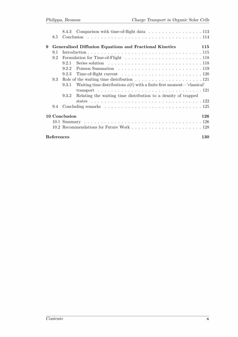
9 Generalised Diffusion Equations and Fractional Kinetics 1159.1 Introduction . . . . . . . . . . . . . . . . . . . . . . . . . . . . . . . . . . 1159.2 Formulation for Time-of-Flight . . . . . . . . . . . . . . . . . . . . . . . 118
9.2.1 Series solution . . . . . . . . . . . . . . . . . . . . . . . . . . . . 1189.2.2 Poisson Summation . . . . . . . . . . . . . . . . . . . . . . . . . 1199.2.3 Time-of-flight current . . . . . . . . . . . . . . . . . . . . . . . . 120
9.3 Role of the waiting time distribution . . . . . . . . . . . . . . . . . . . . 1219.3.1 Waiting time distributions ϕ(t) with a finite first moment—’classical’
transport . . . . . . . . . . . . . . . . . . . . . . . . . . . . . . . 1219.3.2 Relating the waiting time distribution to a density of trapped
states . . . . . . . . . . . . . . . . . . . . . . . . . . . . . . . . . 1229.4 Concluding remarks . . . . . . . . . . . . . . . . . . . . . . . . . . . . . 125
10 Conclusion 12610.1 Summary . . . . . . . . . . . . . . . . . . . . . . . . . . . . . . . . . . . 12610.2 Recommendations for Future Work . . . . . . . . . . . . . . . . . . . . . 128
References 130
Contents x

List of Figures
2.1 A current-voltage curve for a solar cell . . . . . . . . . . . . . . . . . . . 42.2 Standard benchmark solar spectra . . . . . . . . . . . . . . . . . . . . . 52.3 Some common organic semiconducting materials . . . . . . . . . . . . . 62.4 The hopping model of charge transport . . . . . . . . . . . . . . . . . . 72.5 The hopping model of charge transport . . . . . . . . . . . . . . . . . . 102.6 Experimental setup for time-of-flight . . . . . . . . . . . . . . . . . . . . 152.7 Typical current transients measured in time-of-flight experiments . . . . 162.8 Typical dispersive current transits plotted on double logarithmic axes . 172.9 Typical experimental setup for photo-CELIV . . . . . . . . . . . . . . . 18
3.1 A typical measurement circuit for transient experiments . . . . . . . . . 343.2 Spatial discretisation scheme . . . . . . . . . . . . . . . . . . . . . . . . 45
4.1 Photo-CELIV transients experimentally recorded at various light intens-ities . . . . . . . . . . . . . . . . . . . . . . . . . . . . . . . . . . . . . . 50
4.2 Measured photo-CELIV transients with varying laser delay times . . . . 524.3 Simulated photo-CELIV transients at varying light intensities and laser
delay times . . . . . . . . . . . . . . . . . . . . . . . . . . . . . . . . . . 534.4 The amount of charge remaining in the device after the delay time . . . 544.5 Simulated photo-CELIV transients in the case of a unipolar conductor
with deep trap sites pre-populated . . . . . . . . . . . . . . . . . . . . . 554.6 A non-dispersive to dispersive transition in simulated photo-CELIV
transients . . . . . . . . . . . . . . . . . . . . . . . . . . . . . . . . . . . 564.7 Carrier mobilities as a function of delay time . . . . . . . . . . . . . . . 58
5.1 Experimental setup for Resistance dependent PhotoVoltage (RPV) . . . 625.2 Simulated non-dispersive RPV transients . . . . . . . . . . . . . . . . . 635.3 The robustness of the RPV technique against varying photogeneration
profiles . . . . . . . . . . . . . . . . . . . . . . . . . . . . . . . . . . . . . 645.4 The robustness of the RPV technique to optical interference . . . . . . . 645.5 Simulated RPV transients in the case of dispersive transport caused by
shallow traps . . . . . . . . . . . . . . . . . . . . . . . . . . . . . . . . . 655.6 Simulated RPV transients in the case of film charging caused by deep
traps . . . . . . . . . . . . . . . . . . . . . . . . . . . . . . . . . . . . . . 655.7 Current-voltage curves under AM1.5G illumination . . . . . . . . . . . . 665.8 Dispersive time-of-flight transients measured in thick film devices . . . . 675.9 Measured RPV transients for an optimised PCDTBT:PC70BM solar cell 675.10 RPV transients measured using two different laser wavelengths . . . . . 685.11 Electron and hole mobilities measured in PCDTBT:PC70BM solar cells 705.12 RPV measurements on PTB7:PC70BM solar cells . . . . . . . . . . . . . 715.13 Mobilities measured in PTB7:PC70BM solar cells . . . . . . . . . . . . . 725.14 Electron and hole mobilities measured in PCDTBT:PC70BM solar cells 73
xi

Philippa, Bronson Charge Transport in Organic Solar Cells
6.1 Circuit schematic for the High Intensity Resistance dependent Photo-Voltage (HI-RPV) experiment . . . . . . . . . . . . . . . . . . . . . . . . 78
6.2 The impact of the film thickness and light absorption profile on theextracted charge . . . . . . . . . . . . . . . . . . . . . . . . . . . . . . . 79
6.3 The impact of the circuit resistance on the extracted charge from sim-ulated resistance dependent photovoltage experiments . . . . . . . . . . 80
6.4 Simulations of the impact of load resistance on the extracted charge . . 816.5 Numerically predicted extracted charge as a function of load resistance . 836.6 Experimentally measured extracted charge as a function of circuit res-
istance . . . . . . . . . . . . . . . . . . . . . . . . . . . . . . . . . . . . . 85
7.1 Simulated IPC data for various carrier mobility ratios . . . . . . . . . . 907.2 Simulated IPC data for various carrier mobility ratios . . . . . . . . . . 927.3 Simulated IPC data for various recombination coefficients . . . . . . . . 927.4 Simulated IPC data for various recombination coefficients . . . . . . . . 937.5 The impact of optical absorption patterns on IPC simulations . . . . . 947.6 The impact of series resistances on IPC simulations . . . . . . . . . . . . 957.7 The impact of charge trapping . . . . . . . . . . . . . . . . . . . . . . . 977.8 The impact of charge trapping, when the quantity of trapped charge is
limited by the density of available trap sites . . . . . . . . . . . . . . . . 987.9 Experimental results confirming the prediction that non-geminate re-
combination begins when the photocurrent reaches the space chargelimited current . . . . . . . . . . . . . . . . . . . . . . . . . . . . . . . . 100
8.1 Simplified time of flight schematic used in current derivation . . . . . . 1068.2 Impact of the fractional order on the time-of-flight transients . . . . . . 1118.3 Impact of the fractional order on the space-time evolution of the number
density. . . . . . . . . . . . . . . . . . . . . . . . . . . . . . . . . . . . . 1118.4 Space-time evolution of the number density profiles for varying transport
coefficients . . . . . . . . . . . . . . . . . . . . . . . . . . . . . . . . . . . 1128.5 Comparison of the model with experimental transients for trinitrofluorenone-
polyvinylcarbazole . . . . . . . . . . . . . . . . . . . . . . . . . . . . . . 113
9.1 Key processes occurring in the kinetic model. . . . . . . . . . . . . . . . 1179.2 Modelled current transients showing the impact of various waiting time
distributions . . . . . . . . . . . . . . . . . . . . . . . . . . . . . . . . . . 1219.3 Modelled current transients for ideal time of flight experiments using
the waiting time distribution (9.15). . . . . . . . . . . . . . . . . . . . . 123
List of Figures xii
1Introduction
Semiconductor technology has transformed the world. Integrated circuits, micropro-cessors, displays, memories, sensors, solar cells, etc. are all ubiquitous in modernsociety. Yet, most of these technologies are manufactured using the same raw ma-terials, the vast majority being silicon. Silicon is cheap, abundant on the Earth, andwell suited to many applications. However, it requires a large energy input due to itsreliance on high temperature manufacturing processes, and is generally used in theform of a brittle crystal that cannot be bent or twisted.
A new class of semiconductors has emerged that might be able to fill a niche thatsilicon cannot. These are polymers, or in casual terms, “plastics”. Most polymersare insulating, but there are a special class of polymers that are able to conductcharges very effectively. The key is conjugation, which is a sequence of alternatingsingle and double bonds. Conjugation is not limited to polymers; it can also be foundin many other organic molecules. All together, these materials are called organicsemiconductors [10].
Organic semiconductors have attracted tremendous scientific attention because oftheir promise of extremely low-cost fabrication, chemical tunability, and mechanicalflexibility [11–17]. These features would especially benefit solar cells, because organicsemiconductors make it possible to literally “print” a solar module onto a roll of plastic[18]. However, the power conversion efficiency of even the best organic solar cells isstill far below that achieved using other technologies [19]. The performance of organicphotovoltaics needs to be improved if they are to be commercially successful and obtainmarket penetration.
The poor performance of organic electronics is partly due to their poor chargetransport properties. (Charge transport is the mechanism by which electric charges
1

Philippa, Bronson Charge Transport in Organic Solar Cells
are conducted through the device.) To work towards improving charge transport per-formance, it is first necessary to have robust tools for measuring that performance. Aswill be described in the next chapter, classical measurement techniques are not wellsuited to organic photovoltaics.
The objective of this thesis is to develop novel approaches for characterising chargetransport in organic semiconductor devices, and especially organic solar cells. Thisis achieved through joint theoretical-experimental studies. The theoretical work isbased on two major types of model. Firstly, a drift and diffusion numerical simula-tion, which is a well-known modelling approach with a long history of success [20–22].The second modelling approach is the so-called fractional kinetic theory [23, 24]. Theexperimental work is the measurement of charge transport properties in a variety oforganic photovoltaic systems using the techniques that are developed in this thesis.
The structure of this document is as follows. Chapter 2 is a literature review witha focus on organic photovoltaics, measurement techniques, and modelling approaches.Chapter 3 describes the numerical simulation model. Chapter 4 applies the model toa classical measurement technique (photo-CELIV) and addresses some of the limita-tions of that technique. Chapters 5 and 6 report on novel experimental approachesdeveloped as part of this study for measuring mobility (speed of charge transport) andrecombination (between electrons and holes, and hence energy loss during transport),respectively. Chapter 7 applies the model to a very common measurement (photocur-rent as a function of light intensity), and reports on new insights that were gained.Next, the focus shifts towards the second class of modelling that was addressed in thiswork. Chapter 8 presents mathematical advances regarding the analytic solution of acertain type of fractional differential equation for charge transport. Then, Chapter 9applies these mathematical techniques to a novel kinetic model that unifies differenttypes of charge transport under a common framework. Finally, Chapter 10 concludesand makes recommendations for the future.
Chapter 1. Introduction 2

2Fundamentals
This chapter presents a literature review. We begin with some background on the char-acteristics of solar cells in general, before moving onto the history and current statusof organic solar cells. The next topic is charge transport, starting with some funda-mental concepts and a discussion of the important physical processes. Key techniquesfor measuring charge transport properties are reviewed, and then various modellingapproaches are discussed. Some gaps in the current knowledge or weaknesses withcurrent methods are highlighted in order to motivate the rest of the thesis.
2.1 Solar Cell FundamentalsA solar cell is a device that converts light into electric power [25]. The electricalbehaviour of a solar cell is defined by its current-voltage curve [25, 26], called an IVcurve or a JV curve, where the symbol I or i refers to current, J or j refers to currentdensity (current per unit area), and V or v refers to voltage. Often current densityis used (instead of current) because it allows a more direct comparison between solarcells with different surface areas. A solar cell has an asymmetric IV curve, as shownin Figure 2.1. Considering first the “dark” curve (when light is not applied), the solarcell behaves as a diode. In reverse bias, no charge is injected and no current will flow;whereas in forward bias, charge will be injected and current will flow once the voltageexceeds the diode threshold voltage. The distinction between reverse bias and forwardbias is important in charge transport experiments, to prevent (or induce) the electricalinjection of charges, respectively.
When light is applied, the solar cell produces current, as shown by the light curvein Figure 2.1. Useful electrical power P = iv is generated in the region indicated
3

Philippa, Bronson Charge Transport in Organic Solar Cells
Current density
Voltage
jsc
(short
circuit
current)
voc
(open circuit
voltage)
Power output
if FF were 1
Threshold voltage
for injection in
forward bias
vmp
(maximum
power point)
Reverse bias
(no injection)
Forward bias
(injection)
Light
Dark
Figure 2.1: A current-voltage curve for a solar cell. The power generated is indicatedschematically by the area of the green rectangle.
by the grey box. Three key points on the IV curve are the short-circuit current (iscor jsc, when the voltage is zero), the maximum power point (vmp, when the poweroutput is maximised), and the open-circuit voltage (voc, when the current is zero). Themaximum power point is illustrated schematically in Figure 2.1 by area enclosed in thegreen rectangle. The ratio between the actual power produced (the green rectangle)and the product iscvoc is called the fill factor (FF). Specifically,
FF =Pmaxiscvoc
, (2.1)
where Pmax is the power produced at the maximum power point. A fill factor of unitywould indicate a perfectly rectangular IV curve.
The “headline” performance number for a solar cell is its power conversion efficiency(PCE), defined as [27]
PCE =Pout
Pin, (2.2)
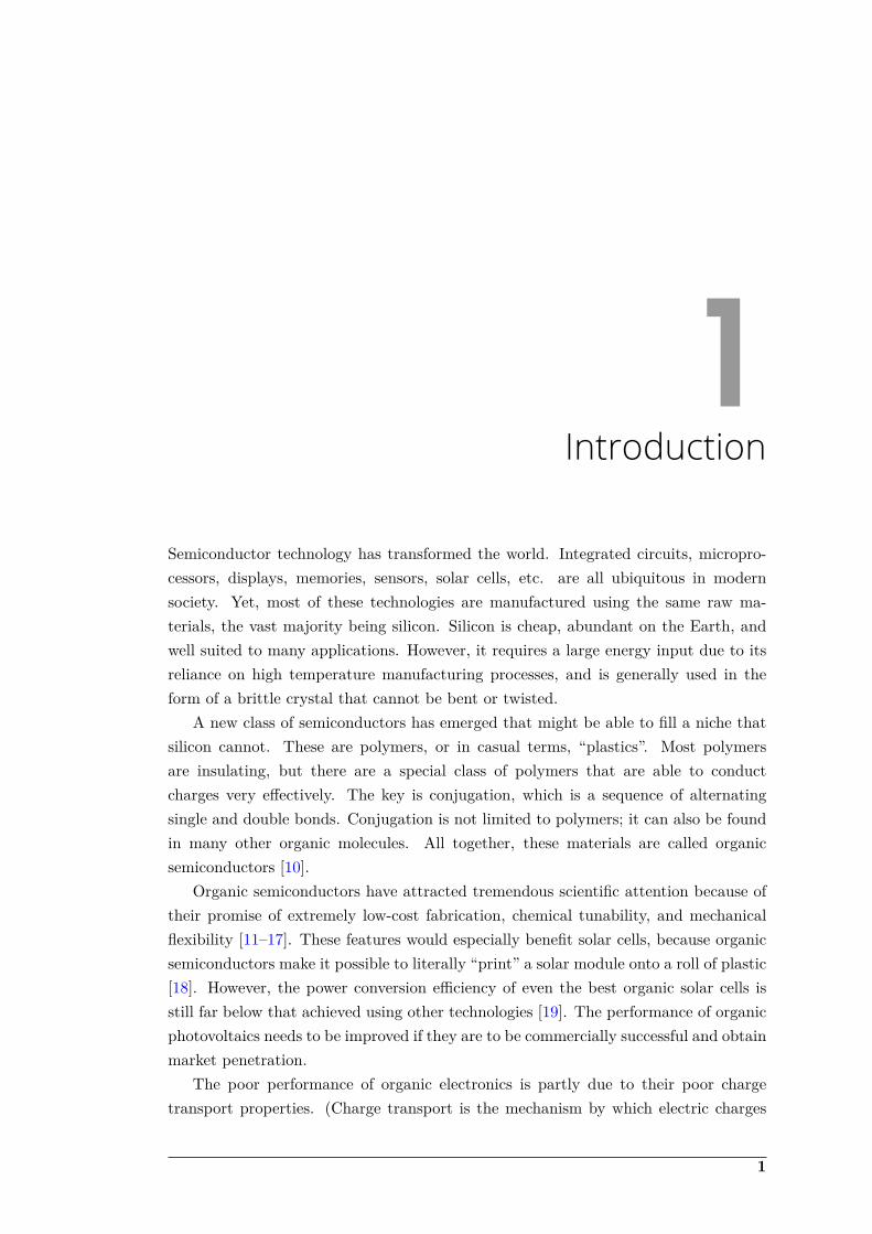
where Pout is the electrical power generated and Pin is the light power incident onthe solar cell. To ensure that PCE measurements are reproducible, it is necessary todefine a standard reference solar spectrum. Natural sunlight is too variable because itdepends upon the position on the Earth, the time of day, etc [25]. The most commonlyused standard is the “AM1.5” spectrum defined by the American Society for Testingand Materials (ASTM) [28], which is plotted in Figure 2.2. Three spectra are shown.The extraterrestrial spectrum is that observed from outside the Earth’s atmosphere; itis also called the “AM0” spectrum because it has been attenuated by zero air masses,where an “air mass” is the thickness of the atmosphere. The AM1.5 spectra representthe solar energy remaining after the sunlight has passed through 1.5 air masses, whichis considered to be a standard reference that accounts for the fact that the sun is notalways perfectly overhead. There are two AM1.5 spectra: the Direct spectrum containsonly that light originating from a small solid angle surrounding the sun, whereas theAM1.5 Global spectrum additionally includes the typical diffuse irradiance caused by
Chapter 2. Fundamentals 4
Philippa, Bronson Charge Transport in Organic Solar Cells
500 1000 1500 2000 2500 3000 3500 40000
0.5
1
1.5
2
2.5
Wavelength (nm)
Spectr
al irra
dia
nce (
W m
−2 n
m−
1)
Extraterrestrial
AM1.5 Global
AM1.5 Direct
Figure 2.2: Standard benchmark solar spectra. The two AM1.5 spectra demonstratethe typical attenuation caused by the atmosphere.
the rest of the sky. For flat solar panels, the AM1.5 Global spectrum is the standardbenchmark.
Not every photon is successfully converted into an electron-hole pair, and not everyelectron-hole pair is successfully transported to their respective electrodes. The com-bined efficiency of the photon-to-extracted-charge-carrier process is called the quantumefficiency of the solar cell. There are two separate quantum efficiencies that are com-monly reported: the Internal Quantum Efficiency (IQE) represents the proportion ofabsorbed photons that result in fully extracted electron-hole pairs; conversely, the Ex-ternal Quantum Efficiency (EQE) represents the proportion of incident photons thatresult in fully extracted electron-hole pairs [27]. The IQE represents the efficiency ofcharge generation and collection in isolation from the optical properties, whereas theEQE also includes the optical reflectance and transmittance of the device. Calculatingthe IQE requires precise optical modelling in order to determine the proportion ofincident photons that are actually absorbed in the active layer [29].
This thesis will examine a new class of emerging solar cells, made from organicsemiconductors. These are discussed next.
2.2 Organic Solar CellsOrganic semiconductors are carbon-rich materials that exhibit semiconducting prop-erties [30]. Interest in these materials often arises because of the belief that they willdeliver substantially reduced costs when compared to conventional, inorganic semicon-ductors [11–14,31,32]. Organic semiconductors also attract attention because they per-mit novel form factors such as lightweight, flexible and transparent electronics [15–17].
The chemical structures of some commonly studied organic semiconducting ma-terials are shown in Figure 2.3. These materials are conjugated, that is, they havechains of alternating single and double bonds. The conjugation causes π orbitals to
Chapter 2. Fundamentals 5

Philippa, Bronson Charge Transport in Organic Solar Cells
PCDTBT
P3HT PCBM
Figure 2.3: Some common organic semiconducting materials. Poly[N-9-heptadecanyl-2,7-carbazole-alt-5,5-(4,7-di-2-thienyl-2,1,3-benzothiadiazole)] (PCDTBT) andPoly(3-hexylthiophene-2,5-diyl) (P3HT) are electron donors, while [6,6]-phenyl-C61-butyric acid methyl ester (PCBM) is an electron acceptor. Images fromSigma-Aldrich.
be delocalised over the conjugated segment, allowing ready charge transport along amolecule and giving rise to interesting electronic properties [10].
There are many applications of organic semiconductors. These include solar cells[33,34], light emitting diodes [35], optically pumped lasers [36,37], thin film transistors[38–41], thin-film memory devices [42], and biosensors [43]. This thesis will focus onorganic solar cells.
The earliest organic solar cells were made using a single active layer [44]. Photo-voltaic effects were observed, but device performance was extremely disappointing (≪1% power conversion efficiency).
The first major development was the bilayer organic solar cell published by Tang in1986 [45]. It improved upon earlier devices by utilising two dissimilar organic semicon-ductors that act as electron accepting and electron donating materials. This conceptis the foundation of modern organic solar cells. The original bilayer device had apower conversion efficiency (PCE) of approximately 1%, and was notable because ofits greatly improved fill factor, demonstrating the benefits of having separate donorand acceptor materials.
The next major development came in 1992 with the report of ultrafast photoin-duced electron transfer from a polymer to a fullerene by Sariciftci, et al [46]. Thatarticle established C60 fullerenes as the prototypical electron acceptor. Nevertheless,
Chapter 2. Fundamentals 6

Philippa, Bronson Charge Transport in Organic Solar Cells
Electron acceptor
Electron donor
-+
CathodeCathode
AnodeAnode
-+
(a) Bilayer (b) Bulk heterojunction
Exciton
Figure 2.4: Two architectures of organic solar cell. (a) A bilayer structure can bemanufactured by sequential deposition of two distinct layers. (b) A bulk heterojunc-tion structure can be manufactured by deposition of a mixed solution. The advantageof the bulk heterojunction structure is that the interfacial surface area is greatly in-creased, improving the overall exciton separation efficiency at the expense of potentialcharge transport problems if there are isolated “islands” that are not connected totheir respective electrode. (The anode and cathode naming convention in solar cellsrefers to the forward bias diode behaviour, even though the desirable photocurrent isin the opposite direction.)
a substantial architectural problem remained. Photogenerated excitations, called “ex-citons”, will only separate with high efficiency if they are able to reach the donor-acceptor interface within their short lifetime (typically 10−10 to 10−9 seconds [47–49]).The original devices had a bilayer structure, as shown in Figure 2.4 (a). Only those ex-citons that were generated near to the interface could contribute to the photocurrent.Bilayer devices are therefore fundamentally limited.
A substantial improvement to the early bilayer devices came with the invention ofthe bulk heterojunction structure, which is a continuous intermixed network of donorand acceptor phases, as shown in Figure 2.4 (b). The idea of this structure is that anexciton should not need to diffuse far before it reaches an interface and can separate.However, the bulk heterojunction introduces new challenges because the domain sizesmust be large enough to ensure that most domains are continuously connected to theirrespective electrode for rapid charge extraction, yet the domains must also be smallenough that excitons can reach the heterojunction. A successful method to form sucha structure was reported in 1995 by Yu et al [50]. The manufacturing process wastantalisingly simple: the two materials were simply mixed in solution and spin cast.This was made possible by the development of the soluble fullerene derivative [6,6]-phenyl-C61-butyric acid methyl ester (PCBM) [51], the structure of which is shown inFigure 2.3. PCBM is still very commonly used to this day [52].
Since these pioneering early publications, the field of organic solar cells has grownenormously. The current PCE record for a single junction organic solar cell is 10.7%[19]. This remains substantially below the record for crystalline silicon cells of 25%[19], and even further behind the GaAs thin film record of 28.8% [19]. However,organic photovoltaics (OPV) still attract interest because of their potential low cost
Chapter 2. Fundamentals 7

Philippa, Bronson Charge Transport in Organic Solar Cells
and innovative form factors. It has been predicted that OPV efficiencies of 20% ormore should be achievable [53].
Some perspective on the modern state of the field can be obtained from a meta-analysis published by Jørgensen, et al [52] in 2013. These authors analysed the status ofOPV by an exhaustive literature survey. Their literature search located 8962 relevantjournal papers, which they claim was the complete record of all OPV publicationsat that time. From these papers they compiled data on 10533 individual organicsolar cells. Overall, the vast majority of devices exhibited performance well below therecord-holding “hero” cells that are commonly cited in performance benchmarks. Theyconcluded that the headline performance numbers are unrepresentative of the majorityof actual devices being produced in laboratories around the world. Consequently,despite the steady improvements in PCE world records, it’s clear that much progressstill needs to be made.
To understand the operational principles of organic solar cells, it’s helpful to followthe sequence of events as a photon is absorbed [54]. As mentioned above, the absorptionof light creates an excited state called an exciton [49] that may move by diffusion untilit reaches the interface between the donor and acceptor phases. At this interface, it isenergetically favourable for the electron to cross from the donor into the acceptor. Theresult is a “charge transfer” (CT) state [49] that consists of a Coulombically boundelectron-hole pair, with the electron in the acceptor and the hole in the donor material.Finally, the charges in the CT state move away from each other, to yield free chargecarriers.
The specifics within the above sequence of events are still under debate [55–61].For a CT state to dissociate into free charges it must overcome a binding energy that isestimated to be an order of magnitude larger than kBT at room temperature [49, 55].(Here, kB is the Boltzmann constant and T the temperature.) Given the apparentlystrong binding energy, it’s somewhat surprising that charge separation occurs at all,let alone with high efficiency.
It has been proposed that above-bandgap light might contribute additional energyto assist with the separation of the CT state [58]. An exciton created by above-bandgaplight is considered to be “hot.” According to this theory, the resulting “hot” CT statesdissociate more readily, using their additional energy to overcome the Coulombic bind-ing energy. However, this theory has been disputed [29, 59, 62]. Quantum yields ofextracted charges have been shown to be independent of the photon energy [59], sug-gesting that “hot” excitons are not actually important for efficient charge generation.Additionally, when optical effects are properly accounted for, some internal quantumefficiency (IQE) spectra are flat [29, 62], further questioning the hot exciton theory.We will return to the question of “hot” carriers in Chapter 5.
It has also been proposed that CT dissociation is assisted by the delocalisationof charge [63], which would assist charge separation by increasing the effective sizeof the CT state and thus weakening the binding energy. Another possibility is thatdissociated charges have higher entropy because a free carrier may sample from a
Chapter 2. Fundamentals 8
Philippa, Bronson Charge Transport in Organic Solar Cells
wider range of possible states, and therefore CT dissociation is assisted by an entropiccontribution [49, 64]. Whatever the mechanism, it is effective, because there existorganic materials with nearly 100% conversion of photons to charge carriers [59, 65].
Once free charge carriers have been created, they must be extracted to the ap-propriate electrodes in order to provide useful energy. This is the process of chargetransport, and it is the main focus of this thesis. Optimal charge transport would movethe charges through the device as quickly as possible, while simultaneously avoidingthe loss of energy through recombination. These steps are discussed below.
2.3 Charge Transport
2.3.1 Semiconducting properties
Conventional semiconductor theory describes transport using a band model [66, 67],with a conduction band and a valence band that are separated in energy. Electronscan be conducted through the material once they are excited from the valence bandinto the conduction band. Similar energetic states exist in organic semiconductors,but due to their chemical structure, the terminology is Highest Occupied MolecularOrbital (HOMO) and Lowest Unoccupied Molecular Orbital (LUMO). The HOMO isthe analogue of the valence band, while the LUMO is the analogue of the conductionband [10,68]. The absorption of a photon can excite an electron from the HOMO intothe LUMO.
The chemical structure of organic semiconductors is such that charge carriers aresubstantially delocalised over conjugated segments of the molecule [69]. This allowscharge to travel very quickly along conjugated segments. However, charge cannot travelso rapidly between conjugated segments [57]. Such a charge transfer will be stronglydependent upon the local spatial and energetic configurations of the respective sites.
An intuitive picture of charge transport in organic materials is that of localisedcharge hopping between sites. A network of sites is distributed in space and energy,as shown in Figure 2.5. Charges move from one site to another by tunnelling or bythermally activated hopping [12,70,71]. If there is an applied electric field, then hopsin the direction of that field will be favourable because the work done by the fieldeffectively lowers the energy of the sites in that direction.
In classical semiconductor theory of ideal systems, there are no energetic statesbetween the conduction band and the valence band. This means that a carrier inthe conduction band cannot thermalise any lower than the conduction band, and willtherefore continue to be able to be conducted for an arbitrarily long period of time.However, defects in the material may result in energetic states between the two bands.These are called “traps”. A carrier that is captured by a trap has dropped out of theconduction band and is no longer able to move. Eventually, thermal fluctuations willimpart enough energy to that carrier that it can be released from the trap and returnto the conduction band. An equivalent situation occurs in the hopping model of Figure
Chapter 2. Fundamentals 9

Philippa, Bronson Charge Transport in Organic Solar Cells
Figure 2.5: The hopping model of charge transport. Carriers occupy sites which aredistributed in energy and position. Movement of charge occurs by hopping events inwhich a carrier rapidly transitions from one site to another.
2.5, where a trap would be a state low enough in energy such that its release time ismuch longer than normal.
The effectiveness of charge transport is often quantified by a parameter called thecarrier mobility. The mobility is the constant of proportionality between the driftvelocity and the electric field, i.e. the velocity is µE where µ is the mobility and Eis the field. A higher mobility is desirable for electronics, since higher-performanceelectronics results from faster-moving carriers. Typical mobilities in organic solar cellmaterials are ∼ 10−5 to 10−3 cm2V−1s−1 [72–75].
2.3.2 Normal transport vs dispersive transport
The hopping model suggests that charge transport results from the chaotic movementof charges throughout a complex spatial and energetic landscape. At the microscopiclevel of individual carriers, some may follow a fortunate sequence of jumps and makerapid motion through the film, while others might take substantially longer [76]. Con-sequently, the classical notion of a carrier mobility is not precisely defined. There’s nosingle velocity that applies to all carriers, because some carriers effectively move fasterthan others at any given moment.
More precisely, charge carrier mobility can no longer be thought of as a invariantmaterial property [77, 78]. The mobility must be subject to a distribution, whichmight be time, position, or temperature dependent [79, 80]. This complicates themeasurement and the modelling of charge transport.
Experimentally, it is not possible to observe the instantaneous velocity distributionbecause the observable conduction current measures only the average motion of allthe charge carriers that are present. The best that can be done is to measure theinstantaneous average velocity. Surprisingly, in some systems, even the average velocityis not always well defined [78], because it is time-dependent and therefore influencedby the geometry of the sample. This is called dispersive transport.
Dispersive transport occurs when the photocurrent reduces with time even beforeany charge carriers have been extracted. The photocurrent results from the averagemotion of all carriers, so this implies that the average velocity is decreasing and/or the
Chapter 2. Fundamentals 10
Philippa, Bronson Charge Transport in Organic Solar Cells
number of carriers is decreasing. This apparent time-dependent mobility makes it dif-ficult to extract a representative value, resulting in an apparent thickness-dependence,where thicker devices have longer transit times and consequently allow more time forthe photocurrent to decay [78]. These issues will be discussed below in relation to theexperimental methods that are commonly applied.
2.3.3 Recombination
Recombination occurs when oppositely charged carriers annihilate [67, 81]. It is theoperational mechanism of light emitting diodes, where radiative recombination eventsgenerate photons. Conversely, recombination is a loss mechanism in solar cells.
Recombination is classified as geminate or non-geminate [82–84]. Geminate re-combination occurs when the recombining electron and hole both originated from thesame photon. It is not necessary that the recombination event occur at exactly thesame location as where the photon was absorbed, because the exciton may diffusesome distance before recombining. Such movement of excitons cannot contribute tothe electrical current because the exciton is not charged.
Non-geminate recombination occurs when the recombining electron and hole haveoriginated from different photons. The electron and hole must physically meet andthen interact. There are various mechanisms by which this can occur, but the simplestis “band-to-band” recombination where two mobile (untrapped) carriers are drawntogether in each other’s electrostatic field. This process is called bimolecular recom-bination and it is described by the rate equation [67,85–87]
∂p
∂t
∣∣∣∣bimolecular recomb.
=∂n
∂t
∣∣∣∣bimolecular recomb.
= −βnp, (2.3)
where n and p are the number density of electrons and holes, respectively. (The numberdensity is the number of charges that are present per unit of volume.)
The prefactor β is the called the bimolecular recombination coefficient. It hasunits of volume per time, and typical values in organic solar cells are 10−13 to 10−11
cm3s−1 [88–91].A simple physical model that aids in understanding the meaning of β is a charge
carrier undergoing random Brownian motion. As it moves, that carrier continuouslysamples the surrounding volume looking for a recombination target. Once it crossesinto the sphere of influence of an opposite charge, it is likely to recombine. Therecombination coefficient β gives the rate at which each carrier samples its surroundingvolume, i.e., volume per time. According to this model, the recombination coefficientis a volume swept per unit time, i.e. β = Svth, where the S is the cross-section forrecombination and vth is the velocity due to thermal motion.
The rate equation (2.3) can be re-written as
∂p
∂t
∣∣∣∣bimolecular recomb.
= − p
τβ, (2.4)
Chapter 2. Fundamentals 11

Philippa, Bronson Charge Transport in Organic Solar Cells
where τβ ≡ (βn)−1 is the bimolecular lifetime. The lifetime gives an approximatelength of time that a carrier is expected to survive before recombination.
Many published organic photovoltaic materials exhibit Langevin recombination[12,92,93], which specifies that the bimolecular recombination coefficient is
βL =e (µp + µn)
ϵϵ0, (2.5)
where e is the charge of an electron, µp and µn are the mobilities of holes and elec-trons, respectively, and ϵϵ0 is the dielectric permittivity. Langevin recombination isderived based on the assumption that transport is the rate limiting step. Chargescannot possibly recombine faster than they can physically meet, and hence Langevinrecombination represents an upper limit on the bimolecular recombination rate.
Some organic photovoltaic devices display recombination coefficients less than theLangevin rate [94–97]. These are called “non-Langevin” materials, and are highlydesirable for efficient photovoltaics.
The derivation of the Langevin rate is usually presented in terms of the Coulombradius [98]. The Coulomb radius (rc) is the distance at which the electrostatic attract-ive potential energy of two charges equals the thermal energy,
V (rc) =e2
4πϵϵ0rc= kT
orrc =
e2
4πϵϵ0kT. (2.6)
The typical argument for the use of the Coulomb radius is as follows. If a chargepasses within a distance rc of another charge, then the mutual attraction of the twocharges will dominate over any tendency for the charges to escape each other (e.g. bydiffusion or an external electric field). It is often suggested [94,99–104] that Langevinrecombination applies if the mean free path is less than the Coulomb radius.
The discussion of the Coulomb capture radius presents a compelling physical pic-ture, but it is not actually necessary in the mathematical derivation. Mathematically,it suffices to take any arbitrary radius and calculate the flux of recombination targetscrossing such a sphere. Consider a frame of reference attached to an electron. In thismoving reference frame, holes have an effective mobility µn+µp. We consider a sphereof radius r centred at this electron, and calculate the flux of holes crossing the spheredue to electrostatic attraction. The physical assumption is that any hole that crossesthis sphere is certain to recombine, i.e. no escape is possible. The holes crossing thesphere move with a velocity (µn + µp)E, where E is the electric field. At a distance rfrom the electron at the origin, the field is given by E = e/4πϵϵ0r
2. Combining these,
flux density per electron = p (µn + µp)E = p (µn + µp)e
4πϵϵ0r2.
Chapter 2. Fundamentals 12

Philippa, Bronson Charge Transport in Organic Solar Cells
Integrating across the surface of the sphere to obtain the total flux, the radius cancels:
recombination flux per electron =ep (µn + µp)
ϵϵ0.
This is the recombination flux due to a single electron. The total recombination rateis obtained by multiplying by the electron number density n,
recombination rate =
[e (µn + µp)
ϵϵ0
]np,
which from Eq. (2.3) allows the Langevin recombination coefficient to be identified:
βL =e (µn + µp)
ϵϵ0. (2.7)
This derivation is independent of the assumed radius r. It is necessary to assumethat the electric field near the electron is given by the electrostatic attraction of thatelectron alone, and this is an approximation that improves with decreasing radius.
The Langevin derivation requires that charges be treated as continuous numberdensities, so that the flux crossing the sphere is density times velocity. It also requiresthat charges be free to move towards each other so that their velocity is µE in thevicinity of the recombination target.
Another recombination mechanism that must be considered is recombination viatrap states [105]. In this mechanism, a charge is first captured into a trap where itbecomes immobilised. At some later time, an oppositely charged carrier may approachand recombine with it. This may be described as “monomolecular” recombination witha first order rate [106,107]
∂p
∂t
∣∣∣∣monomolecular recomb.
= −pτ, (2.8)
where τ is the monomolecular lifetime. The lifetime τ is controlled by the density oftrapped charges. However, this model is too simple for our needs because it does notbalance the recombination rates of both types of charges. According to Eq. (2.8), thehole density p will continue to decay regardless of whether there are any electrons leftin the trap states. This violates the conservation of charge.
The problem of trap-assisted recombination was first solved by Shockley and Read[108] and Hall [109]. The so-called Shockley-Read-Hall (SRH) recombination via elec-tron traps is described by the equations
∂p
∂t
∣∣∣∣SRH recomb.
=∂n
∂t
∣∣∣∣SRH recomb.
= βSRH(np− n1p1) (2.9)
βSRH =CnCpNt
Cn (n+ n1) + Cp (p+ p1), (2.10)
where n1 (p1) is the equilibrium concentration of electrons (holes), Cn is the probabilityper unit time that an electron will be captured by an empty trap, Cp is the probability
Chapter 2. Fundamentals 13

Philippa, Bronson Charge Transport in Organic Solar Cells
per unit time that a hole will be captured by a trapped electron, and Nt is the densityof electron traps. SRH recombination is derived from the principle of detailed balancefor a system in thermal equilibrium.
Instead of the SRH expression, which inherently incorporates the trap capturetime, one might prefer to decouple the recombination model from the trapping modelso that these can be specified in isolation. To achieve this, there are three possiblemechanisms which must be considered [110]:
1. A free electron recombining with a free hole;
2. A free electron recombining with a trapped hole; and
3. A trapped electron recombining with a free hole.
Each mechanism will be second order, proportional to the number density of eachrespective species, i.e., of the form βnp for some recombination coefficient β. It hasbeen shown that the coefficient β may be estimated from the Langevin rate withthe corresponding mobility set to zero [105]. This makes physical sense, because insystems with near-to-Langevin recombination, the limiting process is likely to be chargetransport. We will return to this issue in the following chapter, when we introducerecombination terms into our numerical model.
2.4 Experimental Methods for Characterising ChargeTransport
Characterisation of charge transport in organic semiconductors is challenging becauseof complex dependencies on device geometry, film morphology, electric field, andcharge carrier concentration; consequently, a variety of techniques have been de-veloped [92, 111–115]. This review focusses specifically on those that apply to solarcell geometries, because measurements taken on other geometries (such as transist-ors) can differ dramatically [116] and are not necessarily representative of photovoltaicperformance due to a concentration-dependence in the carrier mobility [117].
2.4.1 Current-voltage curves
Carrier injection (in the dark) can be used to probe charge transport. For the case ofinjection into an ideal undoped, unipolar semiconductor, the Mott-Gurney square lawdescribes the current density as a function of voltage [118]
j =9
8
ϵϵ0µV2
d3, (2.11)
where ϵϵ0 is the permittivity, µ is the mobility, V is the effective voltage (applied plusbuilt-in), and d is the thickness of the semiconductor. If a JV curve has a regimewhere the slope is proportional to V 2, then the mobility can be extracted by fitting
Chapter 2. Fundamentals 14

Philippa, Bronson Charge Transport in Organic Solar Cells
OscilloscopeRload
+-
DCVoltageSupply
Laser pulse
Transparentelectrode
Semiconductorblend
Electrode
Current, i
Figure 2.6: Typical experimental setup for time-of-flight. The laser pulse photogen-erates carriers that subsequently move under the influence of the DC voltage. Theresulting electric current is measured by the oscilloscope and the load resistance Rload.
Eq. (2.11) to the data. When applying this technique, care must be taken to ensurethat the current is not limited by injection barriers or series resistances. Furthermore,a major weakness of this approach is that the presence of charge trapping will modifythe slope of the JV curve [119]. It is possible to calculate j(V ) for certain types oftrapping distribution [118,120], but this requires assumptions or knowledge about thetypes of traps.
Solar cells blends are bipolar conductors, and the Mott-Gurney law does not applyif both types of carrier are present. Nevertheless, it can be used as an approximation ifspecial “hole only” or “electron only” devices are fabricated by using a poorly matchedelectrode that prevents injection of the corresponding type of carrier [104,121]. Chan-ging the electrode material may modify the film morphology, and consequently it isdesirable to measure the mobilities in actual operational devices.
“Double” injection (of both types of carrier) into bipolar devices can also be usedto characterise charge transport [106, 122, 123]. However, the double injection currentdepends upon the mobilities of both carriers, the bimolecular recombination coefficient,and the distribution of traps. Consequently, care must be taken when interpretingdouble injection experiments that all of these dependencies are properly accountedfor. The interpretation is much simpler when the transport of a single type of carriercan be studied in isolation, as is possible with time-of-flight.
2.4.2 Time-of-Flight
The time-of-flight (TOF) technique is a well established method that has been usedfor many years [124, 125]. The experimental setup is shown in Figure 2.6. A DCvoltage is applied to the sample in reverse bias. It is necessary that the sample has avery low conductivity so that the resulting “dark” conduction current in reverse bias isnegligible. A packet of charge carriers is generated near one of the electrodes, typicallywith a nanosecond laser pulse. The DC voltage causes the charge packet to movethrough the semiconductor, and the time of the charge carriers’ “flight” is observed by
Chapter 2. Fundamentals 15

Philippa, Bronson Charge Transport in Organic Solar Cells
Cur
rent
Time
Normal transport
Cur
rent
Time
Dispersive transport
Figure 2.7: Typical current transients measured in time-of-flight experiments, whenthe light intensity is low such that the electric field is not disturbed by space chargeeffects. In the case of normal transport, the plateau reveals the constant velocity ofthe carriers, whereas in the case of dispersive transport, the carrier mobility is poorly-defined.
measuring the electrical current. The velocity of the charges, and hence their mobility,can be calculated with knowledge of the geometry of the sample.
Classical time-of-flight as just described depends upon the smooth and constantmotion of the packet of charge carriers. For this to occur, the electric field inside thedevice must be undisturbed by space charge effects, and so it’s necessary to use a lightintensity low enough that the amount of photogenerated charge is much less than thecharge on the electrodes, CU , where C is the capacitance of the device and U is thevoltage. Note that time-of-flight can also be conducted at high light intensities, inwhich case it provides a measure of charge carrier recombination [89,102].
Schematic representations of typical low-light intensity time-of-flight transientsare shown in Figure 2.7. Normal transport—in which charges move in a coherentpacket—is shown on the left side, whereas dispersive transport—in which the pho-tocurrent continuously decays—is shown on the right side. The flat plateau in thecase of normal transport indicates a packet of charge moving with a constant velocity.Conversely, in the case of dispersive transport, no such plateau is visible.
The apparently featureless dispersive transient usually demonstrates some structurewhen plotted on logarithmic axes, as shown in Figure 2.8. Often there are two powerlaw regimes with slopes −1 + α and −1 − α, respectively, where 0 < α < 1 [77, 78].The dimensionless parameter α describes the severity of the dispersion, with smallervalues of α indicating more severe dispersion. The transition between the two regimesoccurs when the slope changes, and this is often interpreted as a representative transittime, from which mobilities are determined.
The two power law slopes of −1± α were predicted by an influential model due toScher and Montroll called the continuous-time random walk [77]. The details of thismodel will be described in more detail below, but for analysing time-of-flight data itis important to recognise that the two slopes sum to −2, independent of the value ofα. Therefore, the “sum of slopes” is a test that determines whether the transport canbe described by a Scher-Montroll continuous-time random walk.
To obtain meaningful time-of-flight transients like Figures 2.7 and 2.8, it is ne-cessary to photogenerate carriers in only a very thin section of the device near to the
Chapter 2. Fundamentals 16

Philippa, Bronson Charge Transport in Organic Solar Cells
Log
(Cur
rent
)
Log(Time)
Figure 2.8: Typical dispersive current transits plotted on double logarithmic axes. Thetwo regions are labelled with the asymptotic behaviour of the current density (j) as afunction of time (t). The coefficient α describes the degree of dispersion. The changein slope, which is marked by an arrow, is often interpreted as a transit time.
surface. This ensures that all charges travel approximately the same distance, and con-sequently their velocities can be calculated on the basis of the sample’s geometry. Ahighly efficient solar cell will always have a thickness similar to the optical penetrationdepth, because otherwise a substantial portion of the device will not receive light andtherefore will not contribute photocurrent. Even more detrimentally, the additionalthickness beyond the optical penetration depth would serve to delay charge extractionand weaken the electric field by spreading the built-in voltage over a larger thickness.The reduced built-in field would cause charges to “pile up” inside the device, increas-ing recombination losses. Consequently, good solar cells are necessarily too thin forclassical time-of-flight. If the devices are made thicker, then the film morphology ormicrostructure may change [126,127], and so time-of-flight is not well suited here.
2.4.3 CELIV
Charge extraction by linearly increasing voltage (CELIV) addresses some of the diffi-culties associated with the standard time-of-flight technique. It was originally used inthe dark to measure mobilities in doped semiconductors [128], and was later extendedto use laser photogeneration [129] or LED photogeneration [72]. When photogenera-tion is used, the technique is called photo-CELIV. Conversely, the name dark-CELIVis sometimes used to explicitly indicate the absence of photogeneration. As shown inFigure 2.9, the experimental setup is similar to time-of-flight, except that the chargesare linearly accelerated by a rising voltage.
A CELIV or photo-CELIV transient contains several features, which are shown inFigure 2.9. There is a displacement current i0 and corresponding current density j0
caused by capacitive charging with a linearly increasing voltage. The displacementcurrent i0 = AC, where A is the slope of the applied voltage and C is the capacitanceof the device. Superposed with the displacement current “step” is the conductioncurrent density ∆j. The conduction current displays a maximum jmax at a time tmax.The maximum jmax is the total current at the maximum, whereas ∆jmax refers tothe conduction current only, i.e. ∆jmax = jmax − j0. The mobility is evaluated from
Chapter 2. Fundamentals 17

Philippa, Bronson Charge Transport in Organic Solar Cells
OscilloscopeR load
Function generatorproducing triangle
voltage
Laser pulse
Transparentelectrode
Semiconductorblend
Electrode
Current, i
Cur
rent
dens
ity
Time
j0
Δj
tmax
jmax
Figure 2.9: Typical experimental setup for photo-CELIV (top), and a schematic cur-rent transient (bottom).
the time tmax. The original dark-CELIV theory specified that the mobility should becalculated with [128]
µ =2
3
d2
At2max
, (2.12)
whereas for photo-CELIV [130]
µ =2d2
3At2max
[1 + 0.36∆jmax
j0
] . (2.13)
Other forms of the mobility equation have been proposed [131], and more recently ithas become apparent that proper interpretation of photo-CELIV requires correctionfactors computed via numerical simulations [132,133].
A strong advantage of photo-CELIV is that it can be applied to thin films [92]. Itworks well in the case of volume photogeneration, as occurs in operational solar cells.Additionally, photo-CELIV can conveniently estimate the bimolecular recombinationcoefficient with [100]
β
βL≈ j0
∆jsat, (2.14)
Chapter 2. Fundamentals 18

Philippa, Bronson Charge Transport in Organic Solar Cells
where ∆jsat is ∆jmax at a high enough light intensity that it is saturated. Overall,photo-CELIV has proven itself to be a powerful tool in the study of charge transportin organic semiconductors [6, 134–136]. It has been widely used to elucidate the fun-damental mechanisms of time-, field-, and carrier concentration-dependence in varioussystems [94,103,137–143].
The impact of dispersion on photo-CELIV is unclear. In time-of-flight, there is aqualitative distinction between non-dispersive and dispersive transients. Photo-CELIVdoes not appear to display such a sharp transition. Intuitively, this may be becausephoto-CELIV measurements are performed on much thinner films than time-of-flight,so charge carriers will have less time to relax before they are extracted from the film.Nevertheless, the impact of dispersion deserves further attention, and we will returnto this question in Chapter 4.
A weakness of photo-CELIV is that the widely used formulae (2.12)-(2.14) arebelieved to be inaccurate under certain important operating conditions [21, 22, 131,132, 144]. For example, even in the ideal case of uniform photo-generation, a generalexpression for the mobility cannot be found unless approximations are made [131].Non-uniform light absorption requires numerical correction factors that have been pub-lished only for the special case of Langevin recombination and Beer-Lambert absorp-tion [133]. In the case of thin films—those having an absorption coefficient-thicknessproduct (αd) of 2 or less—the correction factor in the equation to calculate the mo-bility varies by approximately a factor of 50 across the range of ∆j/j0 [133]. If thickfilms are also included, the variation is as much as 100 times. Real devices displaymore complex optical absorption patterns [29], and calculation of the correction factoris therefore more difficult, but the Beer-Lambert case provides an estimate of the sizeof the uncertainty. These correction factors need to be adjusted if the system exhibitsnon-Langevin recombination, and so the uncertainly may be even larger in the caseof strongly suppressed recombination. Charge trapping is another problem for photo-CELIV. A study by Hanfland et al [144] concluded that CELIV mobilities for “typicalorganic solar cells” are only accurate to within one or two orders of magnitude. Overall,it should be expected that photo-CELIV mobilities have an uncertainty of at least anorder of magnitude, and probably more if numeric simulations are not used to supplycorrection factors.
A further problem with photo-CELIV is the unintended extracted of charge bythe built-in field during the delay time between photo-generation and the beginningof the applied voltage ramp [145]. This has been addressed via improvements in theexperimental methodology. A nanosecond switch can be used to hold the device at opencircuit during the delay time [88,146]. Alternatively, the open-circuit voltage transientcan be prerecorded and then “played back” during the delay time to simulate opencircuit conditions [72]. However, even if the electric field were perfectly compensated,there will still be diffusion and recombination during that time, which will influencethe shape of the extraction transient, and hence the measured mobility. This issue
Chapter 2. Fundamentals 19

Philippa, Bronson Charge Transport in Organic Solar Cells
will be addressed in Chapter 4. The weaknesses of the photo-CELIV technique haveinspired the development of the RPV technique (Chapters 5 and 6).
2.4.4 Transient PhotoVoltage (TPV)
The transient photovoltage (TPV) technique measures the lifetime of charge carriersvia a decay in voltage [147]. Typically, a white-light bias is applied to generate anopen-circuit voltage voc, then a small optical perturbation (typically with a pulsedlaser) temporarily increases voc. The decay of this open-circuit voltage voc is recor-ded using an oscilloscope with a large input impedance. It is commonly believed thatthe measured decay in voltage corresponds to the recombination of the additionalcharges that were photogenerated by the optical perturbation [147]. The measuredlifetime depends upon the concentration of charge carriers that are present accord-ing to τβ = (βn)−1, and so the lifetime alone (without analysis of the charge carrierconcentration) is insufficient to quantify the nature of the recombination or to com-pare distinct systems, despite some attempts to do so [148]. It is necessary to obtainthe carrier concentration by other means in order to compare TPV lifetimes betweensystems [149].
The TPV measurement is conducted under open-circuit conditions, where chargecarriers are spatially separated and recombination is suppressed. More importantly,however, the number density n in the lifetime equation τβ = (βn)−1 is likely to bestrongly non-uniform, as indicated by simulations of open circuit conditions [20]. Con-sequently, the spatially-varying lifetime at open circuit greatly complicates the inter-pretation of lifetime measurements [150].
2.5 Models of Charge TransportMicroscopic models of charge transport in organic semiconductors are typically basedon the hopping of charge carriers between localised sites (see, for example, refer-ences [76, 77, 93, 151–158]). These models are remarkably successful in explaining andpredicting charge transport fundamentals, however, they suffer from several problems.Firstly, the model inputs are in terms of microscopic parameters, such as the char-acteristics of the site-to-site hopping mechanisms, and these are difficult to measure.Secondly, these models are computationally expensive, especially since each chargeablesite—and often each individual carrier—is accounted for individually. It is thus dif-ficult to scale these models to a realistic number of sites or a realistic number ofcarriers. Some transport effects (such as space charge limitations) only appear at highconcentrations of charge, and therefore these are difficult to model using a microscopicapproach.
An alternative is a drift-diffusion model [20–22]. These models consider a con-tinuum of charge densities, rather than discrete chargeable sites, and are described bypartial differential equations (PDEs) rather than probabilistic hopping rates. The con-tinuum model’s input parameters are all macroscopically important quantities, such as
Chapter 2. Fundamentals 20

Philippa, Bronson Charge Transport in Organic Solar Cells
carrier mobilities and recombination coefficients. Additionally, there are strong compu-tational advantages because large devices with high charge densities can be simulatedin seconds on a typical computer. A weakness of the continuum models is that anytemperature-, field- or density-dependence must be assumed a priori and inserted asan input parameter [159], whereas microscopic models can often make ab initio pre-dictions of any such dependencies [151]. Additionally, dispersive transport often arisesnaturally in microscopic models, in contrast to standard drift-diffusion models wheredispersive mechanisms must be explicitly included in the model.
2.5.1 Gaussian Disorder Model
Perhaps the most commonly used hopping framework is the Gaussian Disorder Model(GDM) [76, 160–162]. According to this model, the energy levels of the sites follow aGaussian distribution, perhaps because of the central limit theorem where the energyof the sites results from the interaction of a large number of random variables. Thedensity of states is written
g(E) =1√2πσ2
exp(−E2
2σ2
), (2.15)
where E is the energy with respect to the mean of the density of states, and σ is thewidth of the distribution and indicates the level of disorder that is present. The valueof σ is called the diagonal disorder. This model may be simulated with Monte Carlotechniques. A typical implementation will place the sites on a three-dimensional grid,populate some sites with carriers, and then simulate the hopping motion by randomsampling from the probability distribution of allowable hops. To implement such aprocedure, the probability of each possible hop must be calculated. These are usuallyobtained first in terms of the hopping rates, i.e. the number of carriers that would beexpected to make such a hop in a given unit of time.
The most commonly used hopping rates are due to Miller and Abrahams [163].According to the Miller-Abrahams rate, hops upward in energy are penalised by aBoltzmann factor, whereas hops downward in energy receive no additional contribution.Hops are always accompanied by the absorption or emission of phonons. The jumprate is [163]
νij =
ν0e−2αRij exp(−Ej−Ei
kBT
), Ej > Ei
ν0e−2αRij , Ej < Ei,
(2.16)
where νij is the hopping rate from site i (which has energy Ei) to site j (which hasenergy Ej), ν0 is an attempt to hop frequency, α is the reciprocal of the decay lengthof the localised wavefunctions, and Rij is the distance between the two sites.
Monte Carlo simulations are performed by calculating the hop rates νij . Long hopshave vanishing probabilities, and therefore it is only necessary to consider some set ofnearest neighbours as candidate destinations j. At any given instant, an individualcarrier will have many allowable destination sites. We introduce the label n to stand for
Chapter 2. Fundamentals 21

Philippa, Bronson Charge Transport in Organic Solar Cells
a particular combination of source and destination indices, i and j respectively. Then,to calculate the hop which is actually taken, we consider the following distribution [164]:
P (τ, n)dτ = P (the next hop is type n AND it occurs within a time interval τ to τ+dτ).
This distribution can rewritten as the product of two factors:
P (τ, n)dτ = P (no hops of any type occuring before time τ)
× P (hop of type n occuring in the interval τ to τ + dτ).
The second factor can be immediately written down. The probability of a hop n
in the differential time interval dτ is νndτ, where νn is the rate constant for the hop oftype n.
To calculate the first factor, we consider the probability that the hop does not occurin the (arbitrarily large) length of time τ by dividing this interval into K segmentsof width τ/K. In each such segment, the probability of the hop not occurring is1 − νnτ/K, to first order in K−1. Then the probability that the hop does not occurin the entire interval of length τ is the product of all these probabilities, in the limitof large K:
P (hop n not occurring in t to t+ τ) = limK→∞
[1− νnτ
K
]K= exp (−νnτ) .
It follows that the probably that no hop at all occurs is the product over all possibletypes
P (no hops of any type occurring in t to t+ τ) =∏m
exp (−νmτ)
= exp(−∑m
νmτ
).
This gives the distribution P (τ, n)dτ as
P (τ, n)dτ = exp(−∑m
νmτ
)νndτ. (2.17)
This distribution is not normalised because it is not certain that the next hop is infact of type n. Summing over all n yields a normalised distribution.
A Monte Carlo simulation will sample from Eq. (2.17) to evaluate the hop takenby each carrier. As the number of carriers increases, the conduction current willconverge to the macroscopic average. The macroscopic conduction current resultingfrom this simple model contains surprisingly rich behaviour [165, 166]. The chargecarrier mobility varies with the energetic configuration of the sites, the electric field,and the temperature [76,167,168]. The results are sensitive to short-range correlations
Chapter 2. Fundamentals 22
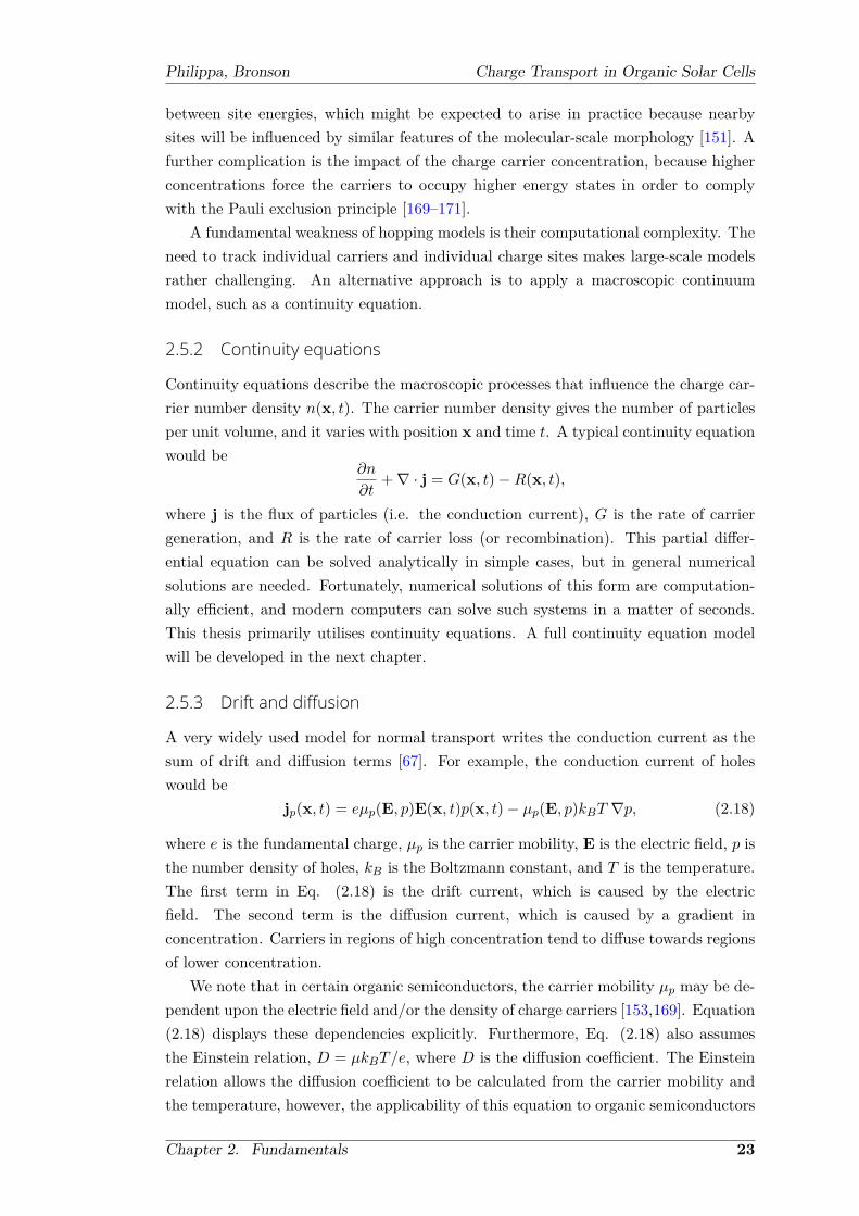
Philippa, Bronson Charge Transport in Organic Solar Cells
between site energies, which might be expected to arise in practice because nearbysites will be influenced by similar features of the molecular-scale morphology [151]. Afurther complication is the impact of the charge carrier concentration, because higherconcentrations force the carriers to occupy higher energy states in order to complywith the Pauli exclusion principle [169–171].
A fundamental weakness of hopping models is their computational complexity. Theneed to track individual carriers and individual charge sites makes large-scale modelsrather challenging. An alternative approach is to apply a macroscopic continuummodel, such as a continuity equation.
2.5.2 Continuity equations
Continuity equations describe the macroscopic processes that influence the charge car-rier number density n(x, t). The carrier number density gives the number of particlesper unit volume, and it varies with position x and time t. A typical continuity equationwould be
∂n
∂t+∇ · j = G(x, t)−R(x, t),
where j is the flux of particles (i.e. the conduction current), G is the rate of carriergeneration, and R is the rate of carrier loss (or recombination). This partial differ-ential equation can be solved analytically in simple cases, but in general numericalsolutions are needed. Fortunately, numerical solutions of this form are computation-ally efficient, and modern computers can solve such systems in a matter of seconds.This thesis primarily utilises continuity equations. A full continuity equation modelwill be developed in the next chapter.
2.5.3 Drift and diffusion
A very widely used model for normal transport writes the conduction current as thesum of drift and diffusion terms [67]. For example, the conduction current of holeswould be
jp(x, t) = eµp(E, p)E(x, t)p(x, t)− µp(E, p)kBT ∇p, (2.18)
where e is the fundamental charge, µp is the carrier mobility, E is the electric field, p isthe number density of holes, kB is the Boltzmann constant, and T is the temperature.The first term in Eq. (2.18) is the drift current, which is caused by the electricfield. The second term is the diffusion current, which is caused by a gradient inconcentration. Carriers in regions of high concentration tend to diffuse towards regionsof lower concentration.
We note that in certain organic semiconductors, the carrier mobility µp may be de-pendent upon the electric field and/or the density of charge carriers [153,169]. Equation(2.18) displays these dependencies explicitly. Furthermore, Eq. (2.18) also assumesthe Einstein relation, D = µkBT/e, where D is the diffusion coefficient. The Einsteinrelation allows the diffusion coefficient to be calculated from the carrier mobility andthe temperature, however, the applicability of this equation to organic semiconductors
Chapter 2. Fundamentals 23

Philippa, Bronson Charge Transport in Organic Solar Cells
has been disputed [172]. Nevertheless, the Einstein relation does appear to be validunder conditions near to thermal quasi-equilibrium [173], as would occur in opera-tional solar cells. For this reason we have written Eq. (2.18) with the Einstein relationincluded. However, if the Einstein relation does not apply, then the variation can bemodelled by simply inserting a prefactor into the diffusion term [174].
To apply this model, the conduction current (2.18) forms the transport term in acontinuity equation. It is coupled with a similar continuity equation for electrons, andthen the electric field is calculated using the Poisson equation. A complete descriptionof such a model and its software implementation is provided in the following chapter.
These models are very widely used [105,159,174–182]. They are simple and compu-tationally efficient. Nevertheless, they do not account for dispersive transport, whichis often present in organic materials, unless further terms are added. One mechanismto implement dispersive transport is the multiple trapping model.
2.5.4 Multiple trapping
The multiple trapping model makes a distinction between free and trapped charge [183].Free charges are considered to be propagating according to standard drift and dif-fusion, but there exists a mechanism whereby a free charge can become trapped.Trapped charges are immobile, until they are released by some physical process (typ-ically thermal activation), whereupon they continue their motion as before.
Multiple trapping models can be formulated in terms of a discrete set of traplevels [184]
∂n
∂t+∇ · j =
∑i
− n
τc,i+niτr,i
(2.19)
∂ni∂t
=n
τc,i− niτr,i
, (2.20)
where n is the number density of free carriers, j is the flux of carriers, ni is the numberdensity of carriers in the ith trap state, τc,i is the capture time for the ith trap, and τr,iis the release time for the ith trap.
Multiple trapping models can also be formulated in terms of a continuum of traplevels [185]
∂n
∂t+∇ · j =
ˆ 0
−∞−νcg(ϵ)n+ νre
ϵ/kBTnt(ϵ) dϵ (2.21)
∂nt(ϵ)
∂t= νcg(ϵ)n− νre
ϵ/kBTnt(ϵ), (2.22)
where g(ϵ) is the density of trap sites, νc is a capture rate, νr is a release rate, andnt(ϵ) is the number density of trapped sites at energy ϵ. Here, energies are measuredwith respect to the conduction band, i.e. ϵ = 0 is the edge of the conduction band andmore negative energies represent states lower in energy. Carriers are thermally excitedout of their localised states, and deeper traps have concomitantly slower release rates.
Chapter 2. Fundamentals 24

Philippa, Bronson Charge Transport in Organic Solar Cells
The above formulations implicitly assume that the charge concentration is lowcompared with the number of trap sites, because the rate of trapping does not considerthe amount of charge already trapped. If the number of charges becomes comparablewith the number of trap sites, then “trap filling” effects need to be included. Trap fillingcan be modelling by introducing a factor of the form 1 − f , where f is the fractionaloccupancy of the trap site [185]. This causes the equations to become nonlinear.
Multiple trapping can model dispersive transport if the density of states g(ϵ) ischosen correctly. Carriers relaxing within an exponential density of states exhibitdispersive transport with a temperature dependent dispersion parameter α = T/Tc,where Tc represents the width of the exponential density of states [184,186,187]. Otherdensity of states distributions may give rise to alternative behaviour. Further detailsof multiple trapping and its implementation are discussed in the following chapter.
2.5.5 Continuous time random walks
The continuous time random walk (CTRW) was an early model for dispersive trans-port that has been particularly influential [77, 188–190]. This is a microscopic schemewhere carriers make random hops in space. Crucially, the time between hops is alsorandom. The scheme is described by a probability density function (pdf) ψ(z, t), whereψ(z, t)dzdt is the probability of a jump of length z to z+ dz occurring after a delay ofduration t to t+ dt.
To analyse a CTRW, we define the waiting time (or hopping time) pdf ϕ(t) andjump length pdf λ(z) as:
ϕ(t) =
ˆψ(z, t)d3z, λ(z) =
ˆ ∞
0ψ(z, t)dt, (2.23)
where the integration with respect to z is taken over the full extent of all spatialcoordinates in the relevant coordinate system.
It is possible to solve this scheme analytically [191]. To do this, we introduce thepdf η(z, t), which is the probability of just having arrived at a point z. The probabilityof arriving at a point z at time t is the combined probabilities of all the jumps thatcould terminate there. This is the integral over all possible jump lengths and times,
η(z, t) = δ(t)p0(z) +ˆ ˆ t
0η(z′, t′)ψ(z − z′, t− t′)dt′d3z′, (2.24)
where p0(z) is the initial condition, that is, the probability of finding a carrier atposition z at time t = 0. As above, the integral over z′ is taken over the full extentof all the spatial coordinates. Recognising that the integrals are convolutions, we are
Chapter 2. Fundamentals 25

Philippa, Bronson Charge Transport in Organic Solar Cells
motivated to take a Laplace-Fourier transform1 to algebraically solve for η:
η(k, s) = p0(k) + η(k, s)ψ(k, s)
η(k, s) =p0(k)
1− ψ(k, s) . (2.25)
The probability that a carrier is still located at a position z some time after itinitially arrived there depends upon the survival probability. The survival probabilityis the probability of not hopping away:
Φ(t) = 1−ˆ t
0ϕ(t′)dt′. (2.26)
Combining these, the overall probability density function for a carrier being at a pos-ition z at time t is
p(z, t) =ˆ t
0η(z, t− t′)Φ(t′)dt′. (2.27)
In Fourier-Laplace space,
p(k, s) = η(k, s)Φ(s)
= η(k, s)[1
s− ϕ(s)
s
]=
p0(k)1− ψ(k, s)
1− ϕ(s)
s. (2.28)
Equation (2.28) gives an analytic solution to any CTRW defined by a probability dens-ity function ψ(z, t), where ψ(z, t) is the probability of making a hop with displacementz after a time t, and where ϕ(t) =
´ψ(z, t)d3z is the waiting time distribution. The be-
haviour of this solution depends strongly upon the moments of ψ. For the purposes ofillustration, we now simplify the problem to one spatial dimension. The characteristicwaiting time T and the jump length variance Σ2 are
ϕ(t) =
ˆ ∞
−∞ψ(z, t)dz λ(z) =
ˆ ∞
0ψ(z, t)dt (2.29)
T =
ˆ ∞
0tϕ(t)dt, Σ2 =
ˆ ∞
−∞z2λ(z)dz. (2.30)
Various types of CTRW scheme can be classified according to whether T and Σ2 arefinite or divergent. Classical transport occurs when both T and Σ2 are finite. Anexample of such a system is charge carriers in crystalline semiconductors. The factthat T and Σ2 are finite implies that the pdf ψ(k, s) has the power series expansion inLaplace-Fourier space
ψ(k, s) = 1− sT − iM1k −Σ2k2
2+ ..., (2.31)
1Transformed functions are denoted by explicit dependence on the Laplace variable s and Fouriervariable k. The combined transformation is f(k, s) =
´ ´ t
0f(z, t) exp (−st) exp(−ik · z)dtdz.
Chapter 2. Fundamentals 26

Philippa, Bronson Charge Transport in Organic Solar Cells
where M1 is the first moment of λ(z). We substitute this distribution into the CTRWsolution (2.28), discarding the higher order terms:
n(k, s) =n0(k)
iM1k/T +Σ2k2/2T + s.
Rearranging,
sn(k, s)− n0(k) +iM1k
Tn(k, s) +
Σ2k2
2Tn(k, s) = 0
and inverting the Laplace and Fourier transforms yields
∂n
∂t+M1
T
∂n
∂z− Σ2
2T
∂2n
∂z2= 0.
This is the classical advection-diffusion equation with normal drift and diffusion terms.Consequently, a CTRW with finite moments T and Σ2 obeys a diffusion equation.
Conversely, if T is divergent but Σ2 remains finite, the CTRW describes dispersivetransport [192]. Early development of this model [77, 193, 194] introduced an ad hocwaiting time distribution ϕ(t) ∼ t−α−1 with 0 < α < 1. This model predicts time-of-flight current transients of the form [77],
i(t) ∼
t−1+α, t ≤ ttr
t−1−α, t ≥ ttr,(2.32)
where ttr is the transit time of the carriers. Recall that these are exactly as observedin many dispersive systems, complete with a “sum of slopes” of −2. This model wassuccessfully applied to dispersive transport in a variety of materials [78].
Since the regular diffusion equation cannot describe dispersive transport, it is inter-esting to solve the dispersive CTRW to see what kind of generalised diffusion equationresults. To illustrate, we shall use the following power series expansion with a divergentfirst moment in time [191,195]
ψ(k, s) = 1− (sτ)α − iM1k −Σ2k2
2+ ..., (2.33)
where 0 < α < 1 and τ is a time scale parameter. Using this distribution in the CTRWsolution (2.28),
n(k, s) =sα−1n0(k)
iM1k/τα +Σ2k2/2τα + sα.
Rearranging,
sαn(k, s)− sα−1n0(k) +iM1k
ταn(k, s) +
Σ2k2
2ταn(k, s) = 0. (2.34)
The first two terms are reminiscent of a Laplace-transformed derivative. Indeed,if we put α = 1, then we have the first derivative. However, we previously specified
Chapter 2. Fundamentals 27

Philippa, Bronson Charge Transport in Organic Solar Cells
α to be strictly less than one. We can use fractional calculus to invert this Laplacetransform and obtain a diffusion equation for dispersive transport. We shall introducefractional calculus next, and then return to Eq. (2.34).
2.5.6 Fractional Calculus
A brief aside: the Leibniz notation for a derivative of order n, dnydxn , is suggestive.
The notation itself tempts thoughts about how this expression could be interpretedfor arbitrary values of n. One could consider a “half-derivative”, n = 1
2 . Applyingthe “half-derivative” twice should be equivalent to an ordinary derivative. Indeed,arbitrary orders could be defined.
Modern mathematical tools allow the development of fractional calculus quite suc-cinctly [196,197]. It is easiest to first consider arbitrary orders of integration.
Fractional Integration
We begin by considering the integration identity of the Laplace transform:
Lˆ t
0f(t)dt
=
Lf(t)s
≡ F (s)
s, (2.35)
where L· is the Laplace transform, and the Laplace transform of f(t) is writtenF (s). By repeated application of this identity, one can generalise this expression tothe n-fold integral
L
ˆ t
0
ˆ t
0· · ·ˆ t
0︸ ︷︷ ︸n times
f(t) dt dt · · · dt︸ ︷︷ ︸n times
=F (s)
sn. (2.36)
For clarity of notation, we introduce the integral operator
Int f(t) ≡ˆ t
0
ˆ t
0· · ·ˆ t
0︸ ︷︷ ︸n times
f(t) dt dt · · · dt︸ ︷︷ ︸n times
, n ∈ N+, (2.37)
where N+ = 1, 2, 3, · · · . The Laplace transform of the integral operator is then
LInt f(t) =F (s)
sn. (2.38)
The expression on the right hand side could be interpreted as the product of twofunctions, F (s) and s−n. A product in Laplace space is a convolution in the timedomain. Noting that the inverse Laplace transform of s−n is tn−1/(n− 1)!, we have:
Int f(t) =1
(n− 1)!
ˆ t
0(t− τ)n−1 f(τ)dτ. (2.39)
This is the Cauchy formula for repeated integration.
Chapter 2. Fundamentals 28

Philippa, Bronson Charge Transport in Organic Solar Cells
The operator In in Eq. (2.39) was defined for natural numbers n, but one couldenvisage the formal replacement of n by some arbitrary number α. To achieve this,it is necessary to exchange the factorial with the Gamma function. Consequently, wearrive at
Iαt f(t) ≡1
Γ(α)
ˆ t
0(t− τ)α−1 f(τ)dτ, ℜ (α) > 0, (2.40)
which defines the fractional integral. It is necessary that ℜ (α) > 0 for this integral toconverge.
The Laplace space representation is straightforward:
LIαt f(t) =F (s)
sα. (2.41)
Equation (2.40) and its Laplace transform (2.41) define fractional integration. Forexample, a “half-integral” is obtained for α = 1
2 . The Laplace representation (2.41)makes it clear that applying the “half-integral” twice is equivalent to an ordinaryintegral of the first order.
Fractional Derivatives
Fractional integration is elegantly defined by the generalisation of the repeated integ-ration formula (2.39). Unfortunately, there is no corresponding formula for “repeateddifferentiation.” So how to form a fractional derivative?
The solution is to combine ordinary derivatives and fractional integration. To forma derivative of order α, we differentiate m times (where m is the next integer largerthan α), and integrate m − α times. However, the order of application is significant.Integration and differentiation operators do not commute, so we immediately arrive attwo alternative definitions [198],
Riemann-Liouville derivative, RLDαt ≡ dm
dtmIm−αt (2.42)
Caputo derivative, CDαt ≡ Im−α
t
dm
dtm. (2.43)
In general, these two derivatives are different operators. When α becomes an integer,then both types of derivative reduce to the standard operator dm
dtm , because I0t is theidentity operator2.
For the case where 0 < α ≤ 1, these two forms of derivative have the Laplacetransforms
LRLDα
t f(t)
= sαF (s)− limt→0+
I1−αt f(t) (2.44)
LCDα
t f(t)
= sαF (s)− sα−1f(0). (2.45)
Notice that the Riemann-Liouville derivative has a fractional initial condition, whereasthe Caputo derivative has the usual initial condition. It is not always clear how this
2This can be easily seen from the Laplace space definition Eq. (2.41).
Chapter 2. Fundamentals 29
Philippa, Bronson Charge Transport in Organic Solar Cells
fractional initial condition can be obtained from physical measurement, although somemodels do admit such a physical interpretation [199]. Nevertheless, the additional workrequired to define the initial condition is a weakness of Riemann-Liouville formulations.
2.5.7 Fractional diffusion
We are now able to return to the equation in Section 2.5.5 that contained a Laplacetransformed “derivative” that we could not invert. Recall that we were considering theanalytic solution in Fourier-Laplace space of a continuous time random walk describingdispersive transport, which is repeated here for clarity:
sαn(k, s)− sα−1n0(k) + iM1kn(k, s) +Σ2k2
2ταn(k, s) = 0.
We now recognise the first two terms on the left hand side as a Caputo fractional de-rivative. Consequently, we can invert the transforms, and obtain a fractional diffusionequation
C0 D
αt n+
M1
τα∂n
∂z− Σ2
2τα∂2n
∂z2= 0. (2.46)
Here, M1/τα is a generalised drift velocity with units (length) (time)−α, and Σ2/2τα
is a generalised diffusion coefficient with units (length)2 (time)−α. In the limit α→ 1,the classical diffusion equation is recovered.
Equation (2.46) is one of many fraction diffusion equations that have been proposed[23]. The various models can be separated into two main categories, depending uponwhether they model the total charge in the system or only the untrapped charge.
The example above began with a CTRW framework, describing total charge. Theresult is Eq. (2.46), or equivalently [200,201]
C0 D
αt n(x, t) +Wγ
∂n
∂x−DL,γ
∂2n
∂x2= 0. (2.47)
We will return to Eq. (2.47) in Chapter 8, where we will present mathematicaladvances related to its efficient analytic solution. This model can also be cast into theform of a Riemann-Liouville derivative and a source term [24]
RL0 Dα
t n(x, t) +Wγ∂n
∂x−DL,γ
∂2n
∂x2=n(x, 0)t−α
Γ(1− α). (2.48)
Alternatively, if one begins with a multiple trapping framework—describing un-trapped charge—the result is a fractional diffusion equation with a Riemann-Liouvillederivative but no source term [185,202]
RL0 Dα
t +Wγ∂n
∂x−DL,γ
∂2n
∂x2= 0. (2.49)
Chapter 2. Fundamentals 30

Philippa, Bronson Charge Transport in Organic Solar Cells
This equation has a peculiar feature: it does not conserve number density. This isunderstood to represent the permanent loss of charges to deep trap states from whichthey will not be released [203].
Fractional diffusion equations such as these can be solved analytically, often byutilising the Laplace transform or by invoking special functions [204–206].
2.5.8 Kinetic theory
Diffusion equations are extremely popular transport models, however, they are neces-sarily a special case of a more fundamental system. For example, the standard diffusionequation is an approximation to kinetic theory [207]. Kinetic theory describes particledistributions as a function of position and velocity, and is consequently able to cap-ture more of the underlying physics. The relationship between kinetic theory and thediffusion equation is well established. Diffusion equations are valid in the limit of longtimes and small gradients [207]. They are useful because these assumptions are oftenwell met, and their simplicity outweighs their small inaccuracy.
On the other hand, fractional diffusion equation is typically developed from aprobabilistic, random-walk model rather than a kinetic theory. For example, Eq. (2.46)results from the truncation of a power series [Eq. (2.33)]. The type of kinetic modelthat would give rise to a fractional diffusion equation has not been widely studied.Such a model is developed and studied in Chapter 9.
2.6 ConclusionOrganic semiconductors are promising and exciting materials, but they are hamperedby poor performance and complex physics. Experimental characterisation of transportphysics is challenging. Consequently, modelling plays a key role in understandingexperimental results. There are two board categories of model which are used forthis purpose: microscopic models (such as the Gaussian Disorder Model), which trackindividual charges as they hop between sites; and macroscopic models (such as the drift-diffusion equation), which describe the evolution of the number density. Drift-diffusionmodels are advantageous due to their computational efficiency and the macroscopicnature of their input parameters. The development and implementation of a drift-diffusion model will be described in the following chapter.
Chapter 2. Fundamentals 31

3Device Modelling and Numerical
Methods
This chapter describes the development and implementation of a numerical simulationprogram. The model is a one-dimensional generalised drift-diffusion-recombinationsolver that is implemented in MATLAB. Its development begins with specification ofequations that describe drift, diffusion, charge generation, and recombination. Next,we discuss non-dimensionalisation, in which the physical quantities are scaled intodimensionless units, yielding physical insights into the true degrees of freedom of themodel. Finally, the implementation details are presented.
3.1 The One-Dimensional Drift-Diffusion ModelWe are developing a model for thin film devices where the film thickness (d) is muchless than the width or height of the electrodes. As a consequence, almost all of thespatial variation will be confined to the direction normal to the electrodes, which wedefine as x, and consequently a one-dimensional model is a useful approximation. Wespecify that the semiconductor occupies the region 0 ≤ x ≤ d.
The drift-diffusion model [67] asserts that the conduction current density consistsof a drift component and a diffusive component:
jp(x, t) = eµpE(x, t)p(x, t)− µpkBT∂p
∂x(3.1)
jn(x, t) = eµnE(x, t)n(x, t) + µnkBT∂n
∂x, (3.2)
32

Philippa, Bronson Charge Transport in Organic Solar Cells
where jp (jn) is the conduction current density due to holes (electrons), e is the ele-mentary charge, µp (µn) is the mobility of holes (electrons), E is the electric field, p(n) is the number density of holes (electrons), kB is the Boltzmann constant, and T isthe temperature.
We utilised the Einstein relation for the diffusion coefficient, D = µkBT/e, torepresent the diffusion coefficient in terms of the mobility and temperature. Thevalidity of the Einstein relation in organic semiconductors is sometimes disputed [172],but is generally supported [173]. We note that variations from the Einstein relationcould be incorporated by introducing a prefactor to the diffusion terms in Eqs. (3.1)and (3.2) [174].
Applying the principle of conservation of charge, we write continuity equations forelectrons and holes:
∂p
∂t+
1
e
∂jp∂x
= g(x, t)− r(x, t) (3.3)∂n
∂t− 1
e
∂jn∂x
= g(x, t)− r(x, t), (3.4)
where the source-sink terms on the right hand side represent the generation rate g andrecombination rate r.
The electric field E will be specified using Poisson’s equation
∂2V
∂x2=
e(n− p)
ϵϵ0(3.5)
E = −∂V∂x
, (3.6)
where V (x, t) is the electric potential, and ϵϵ0 is the permittivity of the semiconductor.As a voltage reference, we choose V (d), where d is the thickness of the semiconductor:
V (d) = 0. (3.7)
For notational convenience, we define U(t) as the voltage across the semiconductor:
U(t) = V (0, t)− V (d, t) =
ˆ d
0E(x, t)dx. (3.8)
3.1.1 Measurement Circuit
A typical measurement circuit is shown in Figure 3.1. Here, the sample under testis placed in series with a load resistor, and a function generator is used to apply avoltage. The quantity of interest is the current i(t), measured using the load resistorand an oscilloscope. As mentioned above and shown in Figure 3.1, the voltage groundreference is taken to be one of the electrodes.
By applying Kirchhoff’s voltage law to the circuit, we find
Vpsu(t) = U(t) + i(t)R, (3.9)
Chapter 3. Device Modelling and Numerical Methods 33

Philippa, Bronson Charge Transport in Organic Solar Cells
Thin film sample
x = 0 x = d
V(d) = 0
Powersupply
unit
Source, electrode,and other resistances
Measurementresistance
(Load resistance)
Oscilloscope
+
-
Capacitance C
Voltage U
Combined resistancesR
Current i
Figure 3.1: A typical measurement circuit for transient measurements. All circuitresistances are lumped together as R, while the capacitance of the thin film sampleis C. A power supply unit generates a waveform Vpsu(t), which is applied to the RCcircuit. The resulting current is measured using a load resistance and an oscilloscope.
where the symbols are defined in Figure 3.1. The voltage across the thin film sampleU(t) arises due to the charge accumulating on the capacitive plates. The current imust be same everywhere in the circuit, due to Kirchhoff’s current law. It will consistof both a conduction current ic and a displacement current id
i(t) = ic(t) + id(t)
= S
[jn (x1, t) + jp (x1, t) + ϵϵ0
∂E(x1, t)
∂t
], (3.10)
where S is the surface area of the device, jn(x) and jp(x) are the conduction currentdensities for electrons and holes, respectively; and x1 is any point inside the sample.The current must be the same everywhere, so x1 is arbitrary within the range 0 <
x1 < d. Defining the total conduction current density jc = jp + jn, and integratingacross the thickness of the film:
ˆ d
0i(x, t)dx = S
ˆ d
0jc(x, t)dx+ Sϵϵ0
∂
∂t
ˆ d
0E(x, t)dx
⇒ i(t) = S ⟨jc(t)⟩+ C∂U
∂t, (3.11)
where C = Sϵϵ0/d is the geometric capacitance of the device, and the angle bracketsdenote a spatial average.
Combining Eqs. (3.9) to (3.11), we obtain
RCdU
dt= Vpsu(t)− U(t)− ic(t)R, (3.12)
where the conduction current ic(t) = S ⟨jc(t)⟩. Equation (3.12) is the form we will useto incorporate the measurement circuit in the model. In the limit of R → 0, we findVpsu = U . Therefore, in the model, we can “turn off” the effects of the external circuitby setting the parameter R to zero.
Chapter 3. Device Modelling and Numerical Methods 34

Philippa, Bronson Charge Transport in Organic Solar Cells
3.1.2 Photogeneration of carriers
Most experiments involve the photogeneration of carriers. Often, a brief flash of lightis used at the beginning of the experiment. We will model this behaviour by settingthe initial values of n and p according to an optical absorption model [133, 208]. Theinitial condition will be
n(x, 0) = p(x, 0) = QphQ1(x), (3.13)
where Qph is a scaling prefactor that indicates the quantity of photogenerated charge,and Q1(x) is the photogeneration profile normalised such that
´ d0 Q1(x)dx = 1. Note
that Qph implicitly includes the quantum efficiency for free carrier generation. Thespatial profile Q1(x) will be determined by a photogeneration model. For example, theBeer-Lambert law would give
Q1(x) =α
1− e−αde−αx (3.14)
if the photogeneration is from the x = 0 side, or
Q1(x) =α
1− e−αde−α(d−x), (3.15)
if the photogeneration is from the x = d side. Here, α is the absorption coefficient.We should highlight that the numerical solver that implements this model will permitarbitrary specification of the photogeneration profile Q1(x).
Another possible setup is continuous illumination. This will be modelled using ageneration term in the continuity equation:
∂p
∂t
∣∣∣∣photogeneration
=∂n
∂t
∣∣∣∣photogeneration
= G(t)Q1(x), (3.16)
where G(t) gives the light intensity in units of generated charge carriers per unit areaper unit time.
3.1.3 Recombination
There are two types of recombination that need to be considered: geminate and non-geminate [82–84]. Geminate recombination occurs when the recombining carriers ori-ginated from the same photon. Any movement of these carriers cannot contributeto the electrical current, because the net movement of one carrier is perfectly com-pensated by the identical net movement of the other. Consequently, from an electricalperspective, the geminate recombination rate can be incorporated into the quantumefficiency for charge generation (i.e., through Qph). That is the approach that we willtake for this model.
Chapter 3. Device Modelling and Numerical Methods 35

Philippa, Bronson Charge Transport in Organic Solar Cells
Non-geminate recombination includes both band-to-band recombination and trap-assisted recombination. The relevant equations are (Section 2.3.3 and ref. [105])
∂p
∂t
∣∣∣∣recomb.
= − β
βL
e (µn + µp)
ϵϵ0np− β
βL
eµpϵϵ0
ntp (3.17)
∂n
∂t
∣∣∣∣recomb.
= − β
βL
e (µn + µp)
ϵϵ0np− β
βL
eµnϵϵ0
npt (3.18)
∂pt∂t
∣∣∣∣recomb.
= − β
βL
eµnϵϵ0
npt (3.19)
∂nt∂t
∣∣∣∣recomb.
= − β
βL
eµpϵϵ0
ntp, (3.20)
where n and p are the number densities of free electrons and holes, respectively; ntand pt are the number densities of trapped electrons and holes, respectively; β/βLis a prefactor to account for non-Langevin recombination; and e (µn + µp) /ϵϵ0 is theLangevin coefficient.
Note that we have assumed that band-to-band recombination and trap-assistedrecombination are both described by the same reduction factor β/βL. This simplifyingassumption is made on the basis of experimental evidence that trap-assisted recom-bination in certain systems is described by a Langevin-like expression with one of themobilities set to zero [105]. Additionally, this assumption is physically reasonable innear-to-Langevin systems such as most organic solar cells, because the limiting step islikely to be charge transport. However, the model could be easily extended to coverthe case where trap-assisted recombination is governed by a different reduction factor.
3.1.4 Boundary Conditions
Precise modelling of the interface between a metallic electrode and an organic semi-conductor is difficult, primarily because of challenges in quantifying the exact natureof the interface, and fabricating reproducible samples [209,210]. Consequently, we willconsider simplified boundary conditions that represent ideal behaviour. Our intent isto model the bulk transport without the influence of non-ideal boundaries.
For the continuity equations (3.1)-(3.2), there are four boundary conditions thatneed to be specified: two species of charged particle each interacting with two elec-trodes. For each species of charged particle, we can categorise one electrode as the“injecting” boundary and the other electrode as the “extracting” boundary. For ex-ample, holes inject at the boundary where the electric field points into the device,whereas electrons inject at the boundary where the electric field points out of thedevice. With this terminology, we can define several boundary conditions:
Outflow boundary condition—This is the default boundary condition for reversebias experiments such as photo-CELIV (Chapter 4) and RPV (Chapters 5 and 6).This boundary condition allows unimpeded charge extraction, and guarantees thatcharges will escape into the electrode provided that there is an electric field to drivethem. At the extracting boundaries, the current is given by the drift term jp = eµpEp,
Chapter 3. Device Modelling and Numerical Methods 36

Philippa, Bronson Charge Transport in Organic Solar Cells
and similarly for electrons. This is an ideal boundary condition in the sense that thepresence of the boundary does not interfere with the charge carrier density other thanto provide a sink for extracted charges. This boundary condition has been used forideal extracting electrodes in analytic solutions and numerical simulations [122, 133].At the injecting boundaries, the current is set to zero (jp = 0 and jn = 0), becausethat is the ideal case for reverse bias.
Ohmic boundary condition (zero field)—This is the default boundary condition forforward bias experiments that involve the injection of charge carriers. This boundarycondition represents perfect charge injection by specifying that the electric field atthe injecting electrode is zero, because if it were non-zero there would be a currentthat injects more carriers until the field is completely screened. Numerically, theimplementation calculates the number density needed just inside the semiconductorso that the field at the semiconductor-electrode interface satisfies |E| < ϵ where ϵ isa small threshold. This boundary condition was used by Lampert and Mark [118] fortheir analytic solutions of various carrier injection problems. These analytic solutionsare valuable because they can be used to benchmark the accuracy of the numeric solver.The extracting boundaries are the same as for the Outflow case, which matches theanalytic solutions that are available [118].
Ohmic boundary condition (Boltzmann statistics)—As an alternative mechanism toimplement Ohmic injection, the number density at the boundaries can be held fixed, tosimulate Boltzmann statistics where the semiconductor edge is in thermal equilibriumwith the reservoir of charges in the metal [20]. According to this boundary condition,the injecting electrode has the fixed number density
n(0) = Nc, (3.21)
while the extracting electrode has
p(0) = Nc exp(−Egap
kT
),
where Nc is an effective density of states and Egap is the bandgap energy (i.e. thedifference between the LUMO of the acceptor and the HOMO of the donor). In thisboundary condition, the effective density of states Nc becomes a free parameter thatmust be fit from experimental data (such as JV curves).
Blocking boundary condition—The blocking boundary condition is relevant when aninsulating layer contacts the semiconductor, rather than a metal. Blocking boundaryconditions set the current to zero.
Some boundary conditions specify the conduction current, and others specify thenumber density. A combination of these could be specified (e.g. Ohmic injectionat one side of the device and a blocking boundary at the other side), or the systemcould transition from one to another (e.g. when charges are injected and then laterextracted). The dynamic switching between boundary conditions of different typesrequires careful implementation in the code.
Chapter 3. Device Modelling and Numerical Methods 37

Philippa, Bronson Charge Transport in Organic Solar Cells
The boundary conditions for Poisson’s equation are
V (0) = U(t)
V (d) = 0,
where U(t) is the voltage across the semiconductor that is determined via solution ofEq. (3.12).
3.1.5 Summary of Model
The basic one-dimensional semiconductor model developed in this section can be sum-marised by the following system of equations:
jp(x, t) = eµpE(x, t)p(x, t)− µpkBT∂p
∂x(3.22)
jn(x, t) = eµnE(x, t)n(x, t) + µnkBT∂n
∂x(3.23)
ic = ⟨jp + jn⟩S (3.24)∂p
∂t+
1
e
∂jp∂x
= g(x, t)− r(x, t) (3.25)∂n
∂t− 1
e
∂jn∂x
= g(x, t)− r(x, t) (3.26)
g(x, t) = Qgen(t)Q1(x) (3.27)
r(x, t) = βnp (3.28)∂2V
∂x2=
n− p
ϵϵ0(3.29)
E = −∂V∂x
(3.30)
U(t) =
ˆ d
0E(x, t)dx (3.31)
RCdU
dt= Vpsu(t)− U(t)− icR. (3.32)
3.2 Non-DimensionalisationNon-dimensionalisation means that the model equations are converted into a dimen-sionless system of units. Ideally, the parameters should be scaled such that physicallyreasonable values have magnitudes not too far from unity, because such a scaling willmake the numerics easier and more accurate. (Differential equation solvers—especiallyimplicit solvers—work best when all variables are approximately the same order ofmagnitude.) Normalising the model has the added benefit of eliminating redundantdegrees of freedom in the parameter space, and thereby identifying the relationshipsbetween variables.
To perform the normalisation, we need to select reference scales for physical unitssuch as time, voltage, and length. Here, we start with an elegant scaling published by
Chapter 3. Device Modelling and Numerical Methods 38

Philippa, Bronson Charge Transport in Organic Solar Cells
Juška [106,122], and then extend it. In this section, we denote dimensionless quantitieswith a prime.
Voltage scale—The obvious voltage scale for normalisation is the maximum voltagefor CELIV and the applied voltage for TOF and other experiments. However, wewould like to retain the freedom to vary the applied voltage without rescaling otherparameters, if it should be necessary. Therefore, we define a reference voltage Uref asthe voltage scale. We normalise the maximum voltage (for CELIV), or applied voltage(for ToF) in terms of this reference
U ′max =
Umax
Uref.
Almost always we take U ′ref = 1, which corresponds to choosing Umax as the voltage
reference. We normalise all voltages to the reference voltage
U ′ =U
Uref
such that 0 ≤ U ′ ≤ U ′ref is the range of applied voltages for CELIV models and
U ′ = U ′ref is the applied voltage for ToF models.
Length scale—The natural length scale is the width of the sample (d), and wenormalise the position coordinate as x′ = x/d.
Time scale—While the natural time scale is the transit time of carriers, in the caseof CELIV experiments we will instead use the pulse duration, tpulse. This choice ofunits makes it easier to reason about the impact of changing the voltage slope. Bynormalising to tpulse, we can vary the voltage slope without changing the entire systemof units for measuring time. Consequently, we normalise the time coordinate as
t′ =t
tscale
tscale =
tpulse, (CELIV experiment)d2
µpUref, (other experiments).
Charge scale—We use the charge on the electrodes at the reference voltage, Qref =
CUref/Sd to scale units of charge.
3.2.1 Consequences of this system of units
The above system of units requires the normalised electric field to be
E′ =Ed
Uref.
The CELIV voltage slope A = Umax/tscale has normalised value A′ = U ′max. As
mentioned above, we will almost always take A′ = 1.
Chapter 3. Device Modelling and Numerical Methods 39

Philippa, Bronson Charge Transport in Organic Solar Cells
We normalise the number densities to the charge scale
n′ =enSd
CUref=
end2
ϵ0ϵrUref
p′ =epSd
CUref=
epd2
ϵ0ϵrUref,
such that n′ = 1 everywhere in the device would correspond to a charge of CUref
distributed evenly.We also normalise the mobility in terms of the above voltage, time and length
scales:µ′ =
Uref tscaled2
µ.
For time-of-flight and other experiments where tscale = ttr, this system of units requiresµ′ = 1. (More precisely, the faster carrier mobility is 1.) For CELIV experiments, thecase of tpulse = ttr corresponds to µ′ = 2, and therefore realistic CELIV transients willhave µ′ ≥ 2.
We normalise the circuit resistance to the time scale selected above:
R′ =RC
tscale.
This scaling is such that the time-of-flight experiment (where tscale = ttr) operatesin differential mode when R′ ≪ 1 and in integral mode with R′ ≫ 1. Differentialmode is required for classical time-of-flight, in which the measurement circuit doesnot substantially interfere with the measured current. Conversely, in integral mode,the measurement circuit acts as an analog integrator, and the measured signal is theintegral of the TOF transient.
The above normalisations require the dimensionless current to be
i′ =tscaleCUref
i,
while the dimensionless current density is
j′ =tscaleCUref
Sj =tscaleCUref
i.
This implies i′ = j′, i.e. the normalised current and current density are equal.We normalise the recombination rate β to the Langevin rate, that is,
β′ =β
βL,
such that a Langevin material will have β′ = 1, while non-Langevin materials will haveβ′ < 1.
Finally, we define the dimensionless temperature as
T ′ =kBT
eUref.
Chapter 3. Device Modelling and Numerical Methods 40

Philippa, Bronson Charge Transport in Organic Solar Cells
3.2.2 CELIV specifics
In the CELIV experiment, the current can be separated into two components: thedisplacement current caused by the charging of a capacitor with a linearly increasingvoltage, and the conduction current. As discussed in Chapter 2, the displacementcurrent is given by
i0 =dU
dtC = AC
where A is the slope of the applied triangle voltage. In normalised units, i′0 = U ′max,
and almost always U ′max = 1 such that the normalised displacement current is equal
to unity. This is why tpulse (rather than ttr) is the preferred time scale for the CELIVexperiment, because if ttr were the time scale then the displacement current i′0 woulddepend upon the mobility!
Since current and current density are equivalent in this system of units, we alsohave j′0 = U ′
max.
3.2.3 Normalised system of equations
The normalised system of equations are
j′p(x′, t′) = µ′pE
′(x′, t′)p′(x′, t′)− µ′pT′ ∂p
′
∂x′(3.33)
j′n(x′, t′) = µ′nE
′(x′, t′)n′(x′, t′) + µ′nT′∂n
′
∂x′(3.34)
i′c =⟨j′p + j′n
⟩(3.35)
∂p′
∂t′+∂j′p∂x′
= g′(x′, t′)− r′(x′, t′) (3.36)
∂n′
∂t′− ∂j′n∂x′
= g′(x′, t′)− r′(x′, t′) (3.37)
g′(x′, t′) = Q′gen(t
′)Q′1(x
′) (3.38)
r′(x′, t′) = β′(µ′p + µ′n)n′p′ (3.39)
∂2V ′
∂ (x′)2= n′ − p′ (3.40)
E′ = −∂V′
∂x′(3.41)
U ′(t) =
ˆ 1
0E′(x′, t′)dx′ (3.42)
R′ dU′
dt′= V ′
psu(t)− U ′(t)− i′cR′. (3.43)
For the remainder of this chapter, we will drop the primes and write directly innormalised units unless otherwise specified.
Chapter 3. Device Modelling and Numerical Methods 41

Philippa, Bronson Charge Transport in Organic Solar Cells
3.3 Modelling Trapping and DispersionFrom a modelling perspective, we can treat both trapping and dispersion effectsthrough a unified framework. The key insight that makes this possible is that num-ber density can be “partitioned” into distributions that have different mobilities. A“mobility partition” is a partial number density, i.e.
n(x, t) =∑i
ni(x, t), (3.44)
where ni is the number density of particles in the ith mobility partition.Traps are simply mobility partitions with zero mobility, whereas non-trap par-
titions will have a nonzero mobility assigned to them. A mix of shallow and deeptraps (with fast and slow release rates, respectively) can be modelled using multiplepartitions, since the release rates of each partition can be specified independently.Similarly, a distribution of mobilities can be modelled by assigning different mobilitiesto each partition. Consequently, “mobility partitions” are a general framework thatcan implement a variety of physical effects.
To numerically implement mobility partitions, we recognise that they effectivelyintroduce a new dimension to the number density distribution. Number density willbe a function of position, time, and mobility. Discretisation along the mobility axisresults in Eq. (3.44).
It is straightforward to extend the charge transport terms in the continuity equa-tion,
jip = µipEpi + µipT
∂pi
∂x(3.45)
∂pi
∂t+∂jip∂x
= gi − rip, (3.46)
and similarly for electrons. (All equations in this section and for rest of this chapterare written in normalised units.)
The recombination term must be considered carefully, because recombination eventscould occur between any oppositely charged pair of mobility partitions with a rateproportional to the sum of their respectively mobilities. Generalising the trap-assistedrecombination model given by Eqs. (3.17)-(3.20), we write a sum over all possiblerecombination targets:
dpi
dt
∣∣∣∣recomb.
= −∑j
(µip + µjn
)β′pinj . (3.47)
A key assumption here is that the reduction factor β′ ≡ β/βL is the same for allpartitions. There is an experimental justification for this assumption in the case oftrap-assisted recombination, where it has been shown that the recombination rate dueto traps is related to the recombination rate due to free carriers, where the trap-assisted
Chapter 3. Device Modelling and Numerical Methods 42

Philippa, Bronson Charge Transport in Organic Solar Cells
case simply has the appropriate mobility set to zero [105]. In the absence of contraryevidence, we therefore keep the number of free parameters low by assuming the samereduction factor across all partitions.
New terms in the continuity equation are needed to model the movement of chargesfrom one mobility partition to another, for example, the rates of trapping and de-trapping. In general, there might be a net movement of charge between any twomobility partitions i and j,
∂ni
∂t
∣∣∣∣due to partition j
= ν(n)ij = −ν(n)ji (3.48)
where ν(n)ij is the net rate of movement of electrons from partition i to partition j, withthe superscripts (n) used for electrons and (p) used for holes. This rate may be timeand position dependent. For example, if n0 represents free electrons and n1 representstrapped electrons, then ν(n)01 (x, t) is the net rate of trapping.
The inter-partition rate coefficients ν(n)ij (for electrons) and ν(p)ij (for holes) are
calculated by one of the models discussed below. Any one of these models can beturned on for a given simulation, in which case the corresponding portion of code willbe invoked to calculate ν(n)ij (x, t), ν(p)ij (x, t) and the mobilities of each partition µin(x, t)and µip(x, t).
3.3.1 Simple trapping
The simple trapping model includes one free mobility partition and one trapped mo-bility partition with fixed capture and release times. It is the simplest trapping model,and it is described by the equations [211]
∂nf∂t
= −nfτc
+ntτr
(3.49)
∂nt∂t
=nfτc
− ntτr, (3.50)
where nf is the free distribution, nt is the trapped distribution, τc is the capture time,and τr is the release time. Separate capture and release times are specified for eachtype of carrier.
In the notation of mobility partitions, if n0 represents free electrons and n1 repres-ents trapped electrons, then
∂n0
∂t
∣∣∣∣due to partition 1
= ν(n)01 (x, t) = −n
0
τc+n1
τr. (3.51)
3.3.2 Simple trapping with trap filling
The simple trapping with trap filling model introduces a blocking term to describethe filling up of trap states. The simple trapping model is modified by introducing a
Chapter 3. Device Modelling and Numerical Methods 43

Philippa, Bronson Charge Transport in Organic Solar Cells
“blocking factor” proportional to the number of unoccupied trap states that remain[185]
∂nf∂t
= −nfτc
(Nt − ntNt
)+ntτr
(3.52)
∂nt∂t
=nfτc
(Nt − ntNt
)− ntτr, (3.53)
where Nt is the number of available trap states, nf is the free distribution, nt is thetrapped distribution, τc is the capture time, and τr is the release time. Separateparameters (Nt, τc, τr) are again specified for each type of carrier.
Expressed as transition rates between mobility partitions,
∂n0
∂t
∣∣∣∣due to partition 1
= ν(n)01 (x, t) = −n
0
τc
(Nt − n1
Nt
)+n1
τr. (3.54)
3.3.3 Multiple trapping
As described in Section 2.5.4, the multiple trapping model [212–215] considers trapsto be distributed in energy space. The trapped distribution is nt(x, t, ϵ) where ϵ is theenergy below the conduction band. Then, the trapping and de-trapping terms in thecontinuity equation are:
∂nf∂t
=
ˆ 0
−∞
eϵ/kBTnt(ϵ)
τr−g(ϵ)nfτc
dϵ (3.55)
∂nt(ϵ)
∂t= −e
ϵ/kBTnt(ϵ)
τr+g(ϵ)nfτc
, (3.56)
where kB is the Boltzmann constant, T is temperature, τr is a release time, τc is acapture time, and g(ϵ) is the density of trap states. Usually, to model typical dispersivetransport [77] we use an exponential density of states,
g(ϵ) =eϵ/ϵtrap
ϵtrap, (3.57)
where ϵtrap is an energy scale representing the width of the distribution.The numerical implementation requires that this system be discretised in energy
space, each discrete energetic level forming one number density partition. Firstly, it isnecessary to truncate the infinite space to a depth ϵmin at which the density of statesg(ϵ) is sufficiently small. Next, energy space is discretised into the linearly spacedvalues ϵ1, ϵ2, · · · , ϵN separated by a width ∆ϵ, resulting in the transition rates
ν0j =eϵj/kBTnj
τr∆ϵ− g(ϵj)n
0
τc∆ϵ, (3.58)
where n0 is the number density of free carriers, and nj (j ≥ 1) is the number density oftrapped carriers at energy depth ϵj . The numerical discretisation width ∆ϵ is chosen
Chapter 3. Device Modelling and Numerical Methods 44

Philippa, Bronson Charge Transport in Organic Solar Cells
LeftElectrode
RightElectrode
j1 j2 j3 j4 j5 j6 j7
n1 n2 n3 n4 n5 n6
E1 E2 E3 E4 E5 E6 E7
Figure 3.2: Spatial discretisation scheme in the case of six cells. Number densities (n)are defined at cell midpoints, whereas the electric field (E) and current (j) are definedat cell boundaries.
to be sufficiently small that the simulation output is independent of it, i.e. the resultdoes not change as ∆ϵ is reduced.
3.4 Numerical Implementation of Model
3.4.1 Spatial discretisation
Spatial discretisation is done using a finite volume method [216], as shown in Figure 3.2.Number densities are defined at cell midpoints, whereas fluxes and related quantitiesare defined at cell boundaries. The finite volume method was selected because it exactlypreserves the conservation of mass [216]. Additionally, the boundary conditions can beeasily specified in terms of current densities, which as discussed previously are oftenphysically relevant.
Using the finite volume method, continuity equations are written for each cell.These take the form of ordinary differential equations rather than partial differentialequations:
dnidt
=ji − ji+1
∆x+ gi − ri, (3.59)
where ni is the number density in the ith cell, ji is the current density between cellsni−1 and ni, gi is the generation rate and ri is the recombination rate or loss rate. Thegeneration and loss terms also include effects such as trapping and release.
Electric fields are defined at cell boundaries, rather than cell midpoints, because thefinite volume method requires the current densities to be specified at the boundaries.We use a first order upwind scheme [216], where the advective contribution to thecurrent is calculated from the number density of the neighbouring “upstream” cell.The “upstream” cell is the one that charge carriers are leaving, as determined bythe direction of the electric field. The advantage of defining the electric field at theboundary is that it makes it easy to identify the “upstream” cell in regions where theelectric field changes sign.
3.4.2 Time integration
Spatial discretisation results in a large system of ordinary differential equations (ODEs)of the form
M∂y∂t
= f(y, t), (3.60)
Chapter 3. Device Modelling and Numerical Methods 45

Philippa, Bronson Charge Transport in Organic Solar Cells
where M is a constant matrix and f(y,t) is a function of the state vector
y =
n0(x0)
n0(x1)...
n0(xN )
p0(x0)
p0(x1)...
p0(xN )
U
, (3.61)
where U is the voltage across the sample. We have written y for the case of a singlemobility partition. If multiple mobility partitions are present, they are inserted intothe state vector underneath n0 and p0. The Poisson equation and the electric field arenot part of the ODE state y; they are simply evaluated at every time step, i.e. theyform part of the right-hand-side function f(y, t).
The system of equations (3.60) is numerically solved by using the ODE solversbuilt into MATLAB. The implicit scheme ode15s generally achieved the highest per-formance. This solver operates by numerically approximating the Jacobian matrix,i.e. all possible partial derivatives ∂f(yi)/∂yj in the ODE system given by Eq. (3.60).For some problems, the solver would occasionally “stall,” and continuously recalculatethe Jacobian with very tiny step sizes. The cost of recalculating the Jacobian is pro-portional to the square of the number of ODEs, and therefore this operation is costly.Consequently, the following optimisation was implemented.
The solver’s speed is continuously monitored. We define the speed as the amountof ODE time advanced in a given window of real time, i.e. simulated time per second.If the solver’s speed drops below a critical threshold, and certain other heuristics aremet, then the program temporarily switches away from the ode15s solver and onto oneof the explicit solvers. Explicit solvers do not require the use of a Jacobian matrix.Once the explicit solver has advanced the problem past the troublesome point, use ofode15s is resumed. This approach of dynamically switching ODE solvers has turnedout to be tremendously useful in reliably achieving high performance simulations.
To implement solver switching, it was necessary to modify the Application Pro-gramming Interface (API) of the ODE solver. Consequently, custom implementationsof ode15s, ode23, and ode23s were produced. Additionally, the Jacobian finder—whichuses finite differences to numerically approximate the matrix—was reimplemented asa parallel algorithm.
Chapter 3. Device Modelling and Numerical Methods 46

Philippa, Bronson Charge Transport in Organic Solar Cells
3.5 ConclusionThis chapter introduced a model for charge transport in disordered semiconductors.Physical effects including advection, diffusion, space charge, recombination, and trap-ping were introduced and a system of equations was developed. Finally, the numericalimplementation of this system of equations was described. The following four chaptersgo on to apply the numerical solver that was described here.
Chapter 3. Device Modelling and Numerical Methods 47

4Charge Extraction by Linearly
Increasing Voltage (CELIV)
This chapter contains material that has been published in the following journal article:[5] Bronson Philippa, Chellappan Vijila, Ronald D. White, Prashant Sonar, Paul L.
Burn, Paul Meredith, and Almantas Pivrikas. Time-independent charge carrier mobil-ity in a model polymer:fullerene organic solar cell. Organic Electronics, 16, 205 (2015).doi:10.1016/j.orgel.2014.10.047.
This chapter includes experimental data that was measured by Chellappan Vijila.The experimental method is summarised here, and full details are found in the citedpublications. The analysis of the data was performed by me. All other work describedin this chapter is my own.
4.1 IntroductionAs discussed in Chapter 2, photo-CELIV is an attractive tool to study charge transportbecause it uses a diode geometry that is representative of the architectures used inorganic solar cells. However, a key weakness of photo-CELIV is that the experimentalsettings such as the light intensity, applied voltage, or delay time can affect the shapeof the transient and thus the apparent mobility. Variations in the delay time havepreviously been used as evidence of a time-dependent mobility [137, 138]. However,changing the delay time will change the charge carrier concentration and therefore the
48

Philippa, Bronson Charge Transport in Organic Solar Cells
shape of the transient may change [133]. It remains unclear whether the apparent time-dependent mobility that has been observed is a genuine effect or whether the photo-CELIV technique has been misleading due to transport and recombination during thedelay time.
Dispersive transport and in particular charge trapping can also affect the analysisof the photo-CELIV experiment. It has been reported that the CELIV mobility inthe presence of traps is only accurate to within one or two orders of magnitude [144].Dispersive transport, where the photocurrent reduces with time even before chargeextraction, is commonly observed in organic semiconductors with time-of-flight exper-iments [75,217–219]. However, it is not clear how to interpret dispersive photo-CELIVtransients, nor is the impact of dispersion on charge carrier extraction necessarily un-derstood.
This chapter will address these questions through a combined theoretical andexperimental study. We will apply the numeric simulation software that was de-scribed in the previous chapter. We explore the impact of the time delay as wellas the role of traps and dispersive transport on the analysis of photo-CELIV experi-ments and the extraction of the charge mobility. Our study is based on the organicsolar cell blend poly[3,6-dithiophene-2-yl-2,5-di(2-octyldodecyl)-pyrrolo[3,4-c]pyrrole-1,4-dione-alt-naphthalene] (PDPP-TNT) and [6,6] phenyl-C71-butyric-acid-methyl-ester(PC70BM) [220]. Optimised solar cells made made from this blend exhibit power con-version efficiencies in the range of ~ 5% [221]. We will show that the photo-CELIVtechnique is potentially misleading and demonstrate how to avoid these issues.
4.1.1 Summary of solar cell fabrication and experimental methods
Solar cell fabrication followed a previously described procedure [7]. PDPP-TNT (33wt. %) and PC70BM (American Dye Source, 67 wt. %) were dissolved at a totalconcentration of 15 mg/mL in a mixture of chloroform and o-dichlorobenzene (4:1 byvolume), then spin coated onto a cleaned ITO-patterned glass substrate. Next, thesample was heated on a hot plate at 60 °C for 10 minutes to drive off excess solvent.The device was finished with a 100 nm thick aluminium electrode that was depositedby thermal evaporation under a pressure of 10−5 mbar. The thickness of the activelayer was 170 nm as measured with a KLA-Tencor P10 surface profiler. The activearea of the device was 0.04 cm2.
Photo-CELIV measurements were conducted with a pulsed Nd:YAG laser pumpedOPO (Ekspla). The pulse width was < 4 ns, and the repetition rate was 1 Hz. Thesample was excited through the ITO side of the device at a wavelength of 740 nm andan intensity of ∼ 0.06 mJ/cm2. Neutral optical density filters were used to attenuatethe light for the intensity dependent measurements. The temperature of the devicewas controlled with a closed cycle helium cryostat. We reported on the temperaturedependences of these devices in a previous publication [7]. All the measurementsreported here were obtained at 120 K, because the reduced temperature enhances the
Chapter 4. Charge Extraction by Linearly Increasing Voltage (CELIV) 49

Philippa, Bronson Charge Transport in Organic Solar Cells
−5 0 5 10 15 20−10
−5
0
5
10
Time (µs)
Cu
rre
nt
(mA
/cm
2)
2.5 mJ/cm2
0.16 mJ/cm2
0.4 mJ/cm2
0.06 mJ/cm2
0.025 mJ/cm2
Dark
0 0.5 10
1
2
Time (t / tpulse
)
Cu
rre
nt
(j /
j 0
)
Simulated tdelay = 0
Experimental tdelay = 2.5 μs
Figure 4.1: Photo-CELIV transients experimentally recorded at various light intensit-ies. The current maxima (which are marked with symbols) only display a small shift asthe light intensity is increased. This is in contrast with the simulation results shown inthe inset, where the maximum position shifts to extremely short times. Note that thelegend refers to the experimental data only. The simulation results neglect the delaytime, as is common in numerical and analytic treatments of CELIV. The clear qualit-ative differences between the experimental and numerically calculated transients raisethe question of whether the shift in tmax originates from the photophysics of chargetransport or whether it is an artefact of the photo-CELIV technique. This differenceis important and must be accounted for when calculating the carrier mobility usingthe photo-CELIV technique.
dispersive effects that we aimed to study. The locations of the maxima were obtainedfrom the noisy data by smoothing the transients with an adjacent averaging filter.
Simulations were performed using the software described in the previous chapter.We assumed a Langevin bimolecular recombination rate, in accordance with our previ-ous study of these devices [7]. We assumed a carrier mobility ratio of µfasterµslower = 50,although the results are insensitive to this ratio because the faster carrier mobility dom-inates in the case of Langevin recombination. Since the devices are thin (170 nm activelayer), we applied volume photogeneration (i.e. a homogeneous initial photocarrier dis-tribution). Additionally, we assumed that the built-in field is perfectly compensatedby the applied constant offset voltage of 0.5 V during the delay time.
4.2 Effect of the delay time and laser intensityTwo related factors that can affect the photo-CELIV transient are the laser pulseintensity and the delay time. Both parameters influence the concentration of chargecarriers during the CELIV extraction. The light intensity controls the quantity ofphotogenerated charges, whereas the delay time controls how many of these recombinebefore initiation of the CELIV triangular voltage pulse. Carrier mobility has beenshown to depend upon concentration [169], so the photo-CELIV response is likely tochange as the light intensity and/or delay time are varied. However, a more insidious
Chapter 4. Charge Extraction by Linearly Increasing Voltage (CELIV) 50

Philippa, Bronson Charge Transport in Organic Solar Cells
problem is that the shape of the photo-CELIV transient varies with concentration evenif the mobility is constant [133].
Experimentally measured photo-CELIV transients at varying light intensities areshown in Figure 4.1 and the corresponding simulated transients are shown in the in-set. The extraction maxima (tmax) are marked by the symbols, and it can be seen thatthere is a qualitative difference between the experiment and the simulation. Numericalsimulations and analytic results both predict that the time of the extraction maximumtmax should become smaller as the light intensity (or the height of the extraction peak)increases [100, 131–133]. Our simulations demonstrate this effect in the inset, wherethe maxima move into the far top-left corner of the plot. In contrast, the experimentalresults in Figure 4.1 show that tmax decreases (shifts to the left) only slightly beforesaturation is reached. One reason for the difference between the simulations and ex-periment is that the simulations neglect the delay time between photo-generation andthe initiation of the ramp voltage. We note that the delay time is commonly neglectedin theoretical treatments of photo-CELIV [100,132,133], presumably because increas-ing the delay time acts to reduce the concentration, which is equivalent to varying thelight intensity in simple models.
The delay time is typically used in the experiment to prevent the extraction transi-ent from being obscured by the voltage oscillations that are caused by the laser excita-tion. These oscillations are visible in Figure 4.1. Crucially, the system is not “frozen”during the delay period, that is, photo-generated charges will diffuse and recombine,and the subsequent loss of carrier concentration will affect the extraction transient.Consequently, changing the delay time should lead to a change in the maxima, andindeed this effect was observed, as shown in Figure 4.2. The locations of the maximawere found to shift by a factor of approximately two over the range of delay times thatwere measured, despite an unchanging light intensity. This would correspond to achange in mobility by a factor of approximately four if the basic dark-CELIV equationµ = 2d2/3At2max was used [128], where d is the device thickness and A is the rate ofchange of the triangular voltage.
To determine the origin of the delay dependence of tmax observed in Figure 4.2,we simulated tmax as a function of tdelay, as shown in Figure 4.3. If the delay timeis set to zero (as in Figure 4.3a and the inset of Fig. 4.1), the position of tmax shiftsto the left of the dark-CELIV predicted position, with the largest shift at the highestlight intensities. When experimentally relevant delay times are included (as in Figures4.3b and 4.3c), the shift of tmax is reduced particularly at higher light intensities, andthe simulations more closely resemble the experimental results. Thus when comparingphoto-CELIV transients it is important to ensure that there are identical delay timesand excitation intensities used if a valid comparison of trends is to be made.
From Figure 4.3 it can be predicted that the shift in tmax will be most prominent athigh light intensities and short delay times. This can be understood by considering thebimolecular recombination that occurs during the delay time. At high light intensities,the bimolecular recombination is very rapid, so a small change in the delay time results
Chapter 4. Charge Extraction by Linearly Increasing Voltage (CELIV) 51

Philippa, Bronson Charge Transport in Organic Solar Cells
0 5 10 15 200
1
2
3
4
5
6
7
8
Time (µs)
Curr
ent (m
A/c
m2)
tdelay
= 1 µs
tdelay
= 3 µs
tdelay
= 7 µs
tdelay
= 20 µs
tdelay
= 50 µs
Dark
Figure 4.2: Measured photo-CELIV transients with varying laser delay times and alight intensity of 0.06 mJ/cm2. The maxima, which are marked by the symbols, moveto the right with increasing delay time. This could be interpreted as a time-dependentmobility, although we will show in Figure 4.7 that this shift actually originates fromcharge recombination during the delay time.
in a large change in the surviving concentration (Figure 4.4a). Similarly, at long delaytimes, the bimolecular recombination has had sufficient time to eliminate the differ-ences between light intensities, especially when the initial concentration is high (Figure4.4b). Overall, accurate mobility estimation requires that the carrier concentration beapproximately constant at the start of extraction, which can be achieved via low lightintensities and/or longer delay times.
4.3 Effect of traps on the transient shapeThere are three general regimes for transport in organic semiconductors, which includedeep traps, shallow traps, and no traps. Previous reports have shown that localizedtrap states influence the shape of CELIV transients, and hence the interpretation ofresults and calculation of transport parameters [144, 222]. The case of no traps hasalready been examined in Figure 4.3. Next, we consider the case of long-lived traps(deep traps), which we define as traps whose average release time exceeds the transittime of carriers. (The transit time in a CELIV experiment is ttr = d
√2/µA, where
d is the film thickness, µ is the mobility, and A is the slope of the triangle voltage.)In the presence of these long-lived traps, charges may remain within the film after thetransient has concluded. If the traps are sufficiently deep, then trapped carriers maystill be present when the next laser shot is fired. We call this effect “film charging”,because the extracted charges leave behind uncompensated trapped charges. Althoughsuch trapped charges do not contribute to the current, they do disturb the electric
Chapter 4. Charge Extraction by Linearly Increasing Voltage (CELIV) 52
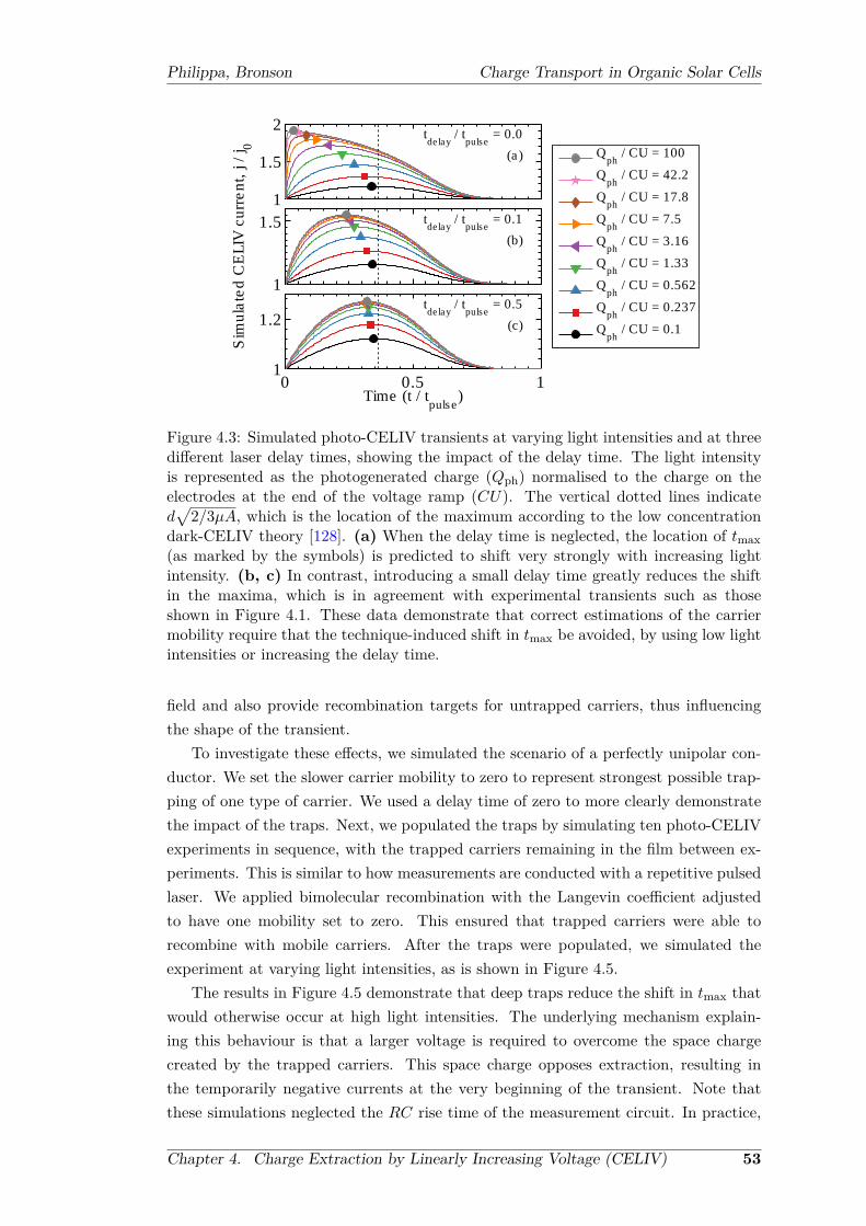
Philippa, Bronson Charge Transport in Organic Solar Cells
1
1.5
2tdelay
/ tpulse
= 0.0
(a)
1
1.5 tdelay
/ tpulse
= 0.1
(b)S
imula
ted C
ELIV
curr
ent, j / j
0
Qph
/ CU = 100
Qph
/ CU = 42.2
Qph
/ CU = 17.8
Qph
/ CU = 7.5
Qph
/ CU = 3.16
Qph
/ CU = 1.33
Qph
/ CU = 0.562
Qph
/ CU = 0.237
Qph
/ CU = 0.1
0 0.5 11
1.2tdelay
/ tpulse
= 0.5
(c)
Time (t / tpulse
)
Figure 4.3: Simulated photo-CELIV transients at varying light intensities and at threedifferent laser delay times, showing the impact of the delay time. The light intensityis represented as the photogenerated charge (Qph) normalised to the charge on theelectrodes at the end of the voltage ramp (CU). The vertical dotted lines indicated√
2/3µA, which is the location of the maximum according to the low concentrationdark-CELIV theory [128]. (a) When the delay time is neglected, the location of tmax(as marked by the symbols) is predicted to shift very strongly with increasing lightintensity. (b, c) In contrast, introducing a small delay time greatly reduces the shiftin the maxima, which is in agreement with experimental transients such as thoseshown in Figure 4.1. These data demonstrate that correct estimations of the carriermobility require that the technique-induced shift in tmax be avoided, by using low lightintensities or increasing the delay time.
field and also provide recombination targets for untrapped carriers, thus influencingthe shape of the transient.
To investigate these effects, we simulated the scenario of a perfectly unipolar con-ductor. We set the slower carrier mobility to zero to represent strongest possible trap-ping of one type of carrier. We used a delay time of zero to more clearly demonstratethe impact of the traps. Next, we populated the traps by simulating ten photo-CELIVexperiments in sequence, with the trapped carriers remaining in the film between ex-periments. This is similar to how measurements are conducted with a repetitive pulsedlaser. We applied bimolecular recombination with the Langevin coefficient adjustedto have one mobility set to zero. This ensured that trapped carriers were able torecombine with mobile carriers. After the traps were populated, we simulated theexperiment at varying light intensities, as is shown in Figure 4.5.
The results in Figure 4.5 demonstrate that deep traps reduce the shift in tmax thatwould otherwise occur at high light intensities. The underlying mechanism explain-ing this behaviour is that a larger voltage is required to overcome the space chargecreated by the trapped carriers. This space charge opposes extraction, resulting inthe temporarily negative currents at the very beginning of the transient. Note thatthese simulations neglected the RC rise time of the measurement circuit. In practice,
Chapter 4. Charge Extraction by Linearly Increasing Voltage (CELIV) 53

Philippa, Bronson Charge Transport in Organic Solar Cells
10−1
100
101
102
10−1
100
101
102
Light intensity (Qph
/ CU)
Ch
arg
e in
th
e d
ev
ice
at
the
sta
rt o
f e
xtr
act
ion
/ C
U
tdelay
/ tpulse
= 0.00
tdelay
/ tpulse
= 0.05
tdelay
/ tpulse
= 0.10
tdelay
/ tpulse
= 0.25
tdelay
/ tpulse
= 0.50
tdelay
/ tpulse
= 0.75
tdelay
/ tpulse
= 1.00
Strong dependence
at high light intensity
Weak dependence
at low light intensity
(a)
10−2
10−1
100
10−2
10−1
100
101
102
tdelay
/ tpulse
Charge in the device at the start of extraction / CU
Qph / CU = 100.00
Qph / CU = 10.00
Qph / CU = 1.00
Qph / CU = 0.10
Qph / CU = 0.01
(b)
Carrier concentration changesstrongly with t
delay
Carrier concentrationis independent of t
delay
Figure 4.4: The amount of charge remaining in the device after the delay time, cal-culated from the solution of the bimolecular recombination equation dn/dt = −βLn2,where n is the carrier concentration and βL is the Langevin recombination coefficient.Light intensity is shown in units of photogenerated charge (Qph) per CU , where CUis the charge on the electrodes at the end of the CELIV triangle voltage. (a) and (b)show two different presentations of the same data.
Chapter 4. Charge Extraction by Linearly Increasing Voltage (CELIV) 54

Philippa, Bronson Charge Transport in Organic Solar Cells
0 0.2 0.4 0.6 0.8 10
0.5
1
1.5 Trap sites were first filled in by tensequential laser shots at Q
ph/CU=10
Time (t / tpulse
)
Cu
rre
nt
(j /
j0)
Qph
/ CU = 300
Qph
/ CU = 100
Qph
/ CU = 30
Qph
/ CU = 10
Qph
/ CU = 3
Qph
/ CU = 1
d
√
2
3µA
Figure 4.5: Simulated photo-CELIV transients in the case of a unipolar conductorwith trap sites pre-populated by immobile carriers whose release time from traps ismuch longer that the transit time of mobile carriers. The vertical dotted lines indicated√
2/3µA, which is the location of the maximum according to the low concentrationdark-CELIV theory [128]. The electric field due to the trapped charges opposes theextraction of the photogenerated charges, eliminating the strong shift in tmax thatoccurs without traps (Figure 4.3a). Consequently, the technique-induced shift in tmaxis not so significant if long-lived traps are present. These simulations neglected RCeffects, and there was no delay time applied.
the very early transients arising due to any trapped charge are not likely to be visiblebecause of the RC rise time and/or the voltage oscillations coincident with the laserpulse.
The trend in Figure 4.5 is reminiscent of that in Figure 4.3b,c in which a timewas introduced. This might explain why some systems display a trend of shifting tmax
while others do not. Devices with sufficient quantities of deep traps will show only aminimal change with light intensity. Thus it is important to quantify the trapping andcharging inside a film, which can be done using methods such as resistance dependentphotovoltage (RPV) [3]. RPV is described in the following chapter.
The final regime to be examined is that of shallow traps that lead to dispersivetransport. While the signature of dispersive transport is often observed in time-of-flightexperiments [77] it is less clear how dispersive transport will influence photo-CELIVtransients. To address this question, we applied a multiple trapping and release modelwith an exponential density of shallow localised states [212–214]. This model extendsthe drift-diffusion equations by including repeated trapping and de-trapping of carriersas they transit through the film. Its advantage is that the dispersive results can bedirectly compared with the non-dispersive results because both are implemented inthe same way. Dispersion arises because of the statistical distribution of trap releasetimes. The severity of the dispersion is controlled by the average depth of the traps,which is quantified by an energy level Etrap/kT , where k is the Boltzmann constant
Chapter 4. Charge Extraction by Linearly Increasing Voltage (CELIV) 55
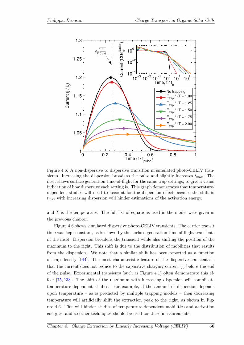
Philippa, Bronson Charge Transport in Organic Solar Cells
0 0.2 0.4 0.6 0.8 11
1.05
1.1
1.15
1.2
1.25
1.3
Time (t / tpulse
)
Cu
rre
nt
(j /
j0)
No trapping
Etrap
/ kT = 1.00
Etrap
/ kT = 1.25
Etrap
/ kT = 1.50
Etrap
/ kT = 1.75
Etrap
/ kT = 2.00
10−3
10−2
10−1
100
101
102
10−4
10−2
100
Time, t / ttr
Cu
rre
nt
(CU
/ttrfa
ste
r )
d
√
2
3µA
Figure 4.6: A non-dispersive to dispersive transition in simulated photo-CELIV tran-sients. Increasing the dispersion broadens the pulse and slightly increases tmax. Theinset shows surface generation time-of-flight for the same trap settings, to give a visualindication of how dispersive each setting is. This graph demonstrates that temperature-dependent studies will need to account for the dispersion effect because the shift intmax with increasing dispersion will hinder estimations of the activation energy.
and T is the temperature. The full list of equations used in the model were given inthe previous chapter.
Figure 4.6 shows simulated dispersive photo-CELIV transients. The carrier transittime was kept constant, as is shown by the surface-generation time-of-flight transientsin the inset. Dispersion broadens the transient while also shifting the position of themaximum to the right. This shift is due to the distribution of mobilities that resultsfrom the dispersion. We note that a similar shift has been reported as a functionof trap density [144]. The most characteristic feature of the dispersive transients isthat the current does not reduce to the capacitive charging current j0 before the endof the pulse. Experimental transients (such as Figure 4.1) often demonstrate this ef-fect [75, 138]. The shift of the maximum with increasing dispersion will complicatetemperature-dependent studies. For example, if the amount of dispersion dependsupon temperature – as is predicted by multiple trapping models – then decreasingtemperature will artificially shift the extraction peak to the right, as shown in Fig-ure 4.6. This will hinder studies of temperature-dependent mobilities and activationenergies, and so other techniques should be used for these measurements.
Chapter 4. Charge Extraction by Linearly Increasing Voltage (CELIV) 56

Philippa, Bronson Charge Transport in Organic Solar Cells
4.4 Time-dependent photocarrier mobilityWith the effects of time delay, light intensity and traps now understood, the questionremains as to how to analyse the photo-CELIV data for the PDPP-TNT:PC70BMblend. The measurements plotted in Figure 4.1 and Figure 4.2 show that tmax moves toshorter times with increasing laser power or decreasing delay time. We can reasonablyassume that the impact of deep traps is minimal because the solar cells are of highefficiency, and the transients more closely resemble the shallow trapping case (Figure4.6) rather than the deep trapping case (Figure 4.5). Since the temperature is constant,the amount of dispersion will remain constant, and so we assume that shallow trapsare unlikely to contribute a time dependence. To justify this assumption, we willshow that recombination during the delay time can entirely predict the observed tmax
shift, so it is not necessary to introduce other time dependencies (e.g. due to trappingor relaxation). We ran simulations across the entire range of delay times that weremeasured, and plotted the resulting tmax values in Figure 4.7a. There is an excellentagreement between the experimental and numerical data, from which we concludethat the observed variation can be entirely explained by charge carrier recombinationduring the delay time. Consequently, the measured trend of an increasing tmax withdelay time is an artefact of the photo-CELIV measurement and is not caused by achanging charge mobility within these devices.
Figure 4.7b compares mobilities calculated directly from tmax with those obtainedfrom fits to simulations. The fitting procedure was to adjust the simulated mobil-ity until the predicted tmax equalled the actual tmax. The crucial difference betweenthe two approaches is that simulation includes recombination during the delay time,whereas the simple mobility equation neglects this effect. We find that there is noevidence of carrier relaxation on transport timescales, in agreement with our previousstudies of charge transport in different organic solar cell blends [3]. The resultantaverage mobility was 2.3 × 10⁻⁵ cm2/Vs, which is similar to our previous report of5× 10−5 cm2/Vs at this temperature (120 K) [7].
4.5 ConclusionVariations in light intensity and delay time can cause substantial shifts in the positionof the CELIV tmax, resulting in apparent changes in mobility. Since the shape of theCELIV transient is sensitive to the concentration of carriers [133], we propose that theshift is caused by recombination during the delay time. In the organic photovoltaicblend studied in this work, we demonstrate that the photocarrier mobility is constanton the time scale of charge extraction, despite a large change in tmax. This suggeststhat photocarrier relaxation effects are insignificant, with any excess energy being loston much shorter time scales. In addition, we studied the impact of shallow traps(causing dispersive transport), and determined that changing amounts of dispersion– as are very likely to occur with changing temperature – will artificially shift the
Chapter 4. Charge Extraction by Linearly Increasing Voltage (CELIV) 57

Philippa, Bronson Charge Transport in Organic Solar Cells
0 10 20 30 40 503
4
5
6
7
8
9 (a)
Delay time (µs)
t max (
µs)
Measurement
Constant mobility, µ = 2.3×10⁻⁵
cm2 V
−1 s
−1
0 10 20 30 40 50
2
4
6
8
10x 10
−5
(b)
Delay time (µs)
Mobili
ty (
cm
2 / V
s)
µ = 2d2/3At
max
2, neglecting t
delay
Fit to tmax
, accounting for tdelay
Figure 4.7: (a) Delay time dependence in the photo-CELIV extraction maximum(tmax). The error bars indicate the time taken for the transients to change by0.05 mA/cm2. (b) Carrier mobilities calculated directly from tmax (red circles), versusmobilities obtained by fitting simulations to tmax (black squares). The shift in tmaxwith delay time (panel a) results in an apparent time-dependent mobility, but thistime dependence is an artefact of the measurement technique, and it disappears whenrecombination during the delay time is properly accounted for (panel b).
position of the CELIV maximum, complicating temperature-dependent studies. Inconclusion, photophysical parameters measured from photo-CELIV, and their trendswhen external parameters are changed, should be estimated with the help of numericalpredictions and simulations.
Chapter 4. Charge Extraction by Linearly Increasing Voltage (CELIV) 58

5Resistance-dependent PhotoVoltage
(RPV)
This chapter contains material that has been published in the following journal article:[3] Bronson Philippa, Martin Stolterfoht, Paul L Burn, Gytis Juška, Paul Meredith,
Ronald D White, and Almantas Pivrikas. The impact of hot charge carrier mobilityon photocurrent losses in polymer-based solar cells. Scientific Reports, 4, 5695 (2014).doi:10.1038/srep05695.
The solar cells studied in this chapter were fabricated by Martin Stolterfoht. Unlessotherwise specified, experimental measurements were conducted by Martin Stolterfohtand Almantas Pivrikas. The analysis of the data was performed by me. All other workdescribed in this chapter is my own.
5.1 IntroductionThe previous chapter reported a study of charge carrier mobility and thermalization us-ing the photogenerated charge extraction by linearly increasing voltage (photo-CELIV)technique. As was discussed in that chapter, the photo-CELIV technique suffers fromvarious limitations, most notably that numerical simulations are required for accurateinterpretation because of the influence of non-uniform photogeneration [133], chargetrapping [144], and a non-uniform electric field [145].
Other measurement techniques also have issues. For instance, the current-voltagemethodology is strongly influenced by trapping [119, 120], while time-of-flight usuallyrequires films that are much thicker than typical high-efficiency operational devices [82,
59

Philippa, Bronson Charge Transport in Organic Solar Cells
223]. These issues inspired the development of the Resistance-dependent PhotoVoltage(RPV) technique that is presented here.
In this chapter, we develop and apply the RPV technique to address the origin ofdispersive transport and the impact of above-bandgap photon energy on the chargeextraction process. Above-bandgap photons create “hot” excitons, the impact of whichon charge generation has been extensively studied [58,224,225]. However, this level ofattention has not extended to studies of the extraction of hot charge carriers, despitethe fact that efficient charge extraction is crucial for device performance [226].
It is important to understand the origin of dispersive transport because it harmsdevice performance by lowering the average photocarrier mobility [227]. Consequently,the vast majority of novel organic semiconductors remain inapplicable for efficientdevices. Moreover, the detrimental effects of dispersion are exacerbated by the in-homogeneities in film thicknesses caused by the targeted low cost deposition method-ologies, because the transit time distributions become dramatically longer and moredispersed in regions of increased thickness.
Dispersive transport in organic semiconductors is usually thought to be causedby the energetic relaxation of hot charge carriers within their density of states [76].Spectroscopic measurements and Monte Carlo simulations have revealed energetic re-laxation extending even to the microsecond timescales, where it could be relevant tobulk charge transport [228, 229]. Even if the bulk of the energetic relaxation were tooccur on very fast timescales, there is still the question of whether residual thermal-ization might continue to long, microsecond timescales. This energetic relaxation isoften understood to cause a time-dependent mobility and therefore explain dispersivecurrent transients [217,230], yet we will show in this chapter that this commonly-usedmodel is inconsistent with our observations in high efficiency organic solar cell ma-terials. Instead, there is an alternative mechanism for the creation of a distributionof carrier velocities, namely, via trapping. This observation has a very direct im-pact on the numerous models, theories and experimental results describing dispersivecharge transport in disordered organic semiconductors. Furthermore, it points to anew strategy for improving charge transport “management” in devices such as organicsolar cells.
The classic signature of dispersive transport is a time-of-flight photocurrent signalthat decays with time even before the carriers have transited through the film [77].This decay in photocurrent can occur due to two mechanisms, a reduction in carriermobility, and/or a reduction in the number (or concentration) of moving carriers.The former, a time-dependent hot carrier mobility, is presently commonly believedto be the cause of dispersion in organic semiconductors [76, 217, 230] and it is usuallyunderstood to originate from a loss of energy as carriers thermalize within their densityof states [231–233]. Higher energy carriers are expected to have a higher hoppingprobability, and hence a higher velocity [151,169,234], so the thermalization within thedensity of states causes the carrier mobility to decline. Recent studies have reportedmobility thermalization times on the order of microseconds [228, 229]. However, an
Chapter 5. Resistance-dependent PhotoVoltage (RPV) 60

Philippa, Bronson Charge Transport in Organic Solar Cells
alternative explanation for the decaying transient photocurrent, which is less commonlyaccepted in organic semiconductors, is a time dependent concentration that can ariseif carriers are gradually lost to traps [141, 212, 213]. The photocurrent signal willcontinue to reduce as long as the net concentration of moving carriers continues todecrease. If that physical process prevails, there can be decaying photocurrent despitethe moving carriers having a constant drift velocity. Additionally, if the cause ofdispersion is trapping, then it will influence all devices, even those which operate inthe dark [73,235].
In this chapter, we demonstrate that a time-dependent hot carrier mobility cannotexplain the dispersive transport in our studied bulk heterojunction solar cells. Weaddress this issue by performing transient photoconductivity experiments in whichwe vary the transit time by changing the electric field and/or device thickness. Theexpectation is that if the dominant cause of dispersive transport is mobility relaxation,then the average mobility and the amount of dispersion should vary with the electricfield and/or film thickness, because longer transit times will allow for more relaxationto occur. Conversely, if the dominant effect is trapping, then it is the concentrationof carriers which is changing in time rather than their mobility, and consequently,the average mobility and the dispersion range should not vary with film thickness orelectric field. This transit time dependence allows these two dispersive mechanisms tobe experimentally distinguished.
5.2 Experimental DesignOur experiments were made possible by the development of a new transient photo-conductivity technique that we call Resistance dependent PhotoVoltage (RPV). Theexperimental measurement circuit for RPV is shown in Figure 5.1. This setup is sim-ilar to time-of-flight, where charge carriers are photogenerated by a short low-intensitylaser pulse. A low light intensity is necessary so that the electric field inside the deviceis undisturbed. The transient photosignal is determined by the competition betweentwo simultaneous processes: the transport of charge carriers inside the film, and theresponse of the external RC circuit. Unique to the RPV approach, and in contrastwith time-of-flight, the entire measurement is repeated at many different load resist-ances spanning the range from differential mode (small R) to integral mode (largeR). The resistance is varied for two reasons: firstly, to visualize the transit times,as will be shown below; and secondly, to reveal the slower carrier mobility by amp-lifying the slower carrier’s conduction current. The slower carriers produce a muchsmaller current than the faster carriers, and their transit would be buried in the noiseat resistances that are optimized for the faster carriers. Slower carriers have muchlonger transit times, allowing the use of larger resistances, and consequently allowingfor their weaker electrical signal to be amplified. In this way, RPV bridges the gapbetween differential mode and integral mode time-of-flight, and allows measurementof the transport of both types of charge carriers.
Chapter 5. Resistance-dependent PhotoVoltage (RPV) 61

Philippa, Bronson Charge Transport in Organic Solar Cells
OscilloscopeRload
+-
DCVoltageSupply
Time
Laser pulse Voltage transients measuredat the oscilloscope for
varying load resistances
Laser pulse
Transparentelectrode
Semiconductorblend
Electrode
Figure 5.1: Experimental setup for Resistance dependent PhotoVoltage (RPV). A lowlight intensity nanosecond laser pulse is used to photogenerate charge carriers insidethe semiconductor junction of an organic solar cell. Low light intensity is critical in theRPV experiment to ensure operation within the “small charge extraction mode” wherethe internal electric field distribution in the film is not altered by transported charges.After photogeneration, the charge carrier transport through the film is driven by thebuilt-in or the applied external electric field, and the resulting transient photosignal isrecorded by an oscilloscope. The transient photosignals are measured at various loadresistances Rload.
The combination of the RC circuit dynamics, dispersive transport, and optical in-terference effects prevent analytic analysis of the transients. To study highly dispersivesystems, such as organic solar cells, the simultaneous impact of all these effects mustbe understood. We applied numerical simulations to develop this understanding, usingthe simulation software that was described in Chapter 3.
5.2.1 Ideal case
Figure 5.2 shows typical transients for the ideal case of no trapping and no dispersion,where the voltage across the load resistance is plotted as a function of time. We use thenotation that V is the voltage on the load resistor and U is the effective voltage acrossthe semiconductor (which is the sum of the built-in voltage and the applied voltage).The results are shown in normalised units, with the load resistance R expressed asRC/ttr(faster), where C is the device capacitance and ttr(faster) is the transit time of thefaster carriers. The transients show two distinct extraction “shoulders,” as indicatedby the arrows. The positions of these arrows correspond to the exact transit timesrequired for the faster and slower carriers to cross the entire thickness of the film. InFigure 5.2, carriers were generated uniformly throughout the film, so there is a spread
Chapter 5. Resistance-dependent PhotoVoltage (RPV) 62

Philippa, Bronson Charge Transport in Organic Solar Cells
10−2
10−1
100
101
102
103
104
105
0
0.25
0.5
0.75
1
Time, t / ttr(faster)
Vo
lta
ge
on
re
sis
tan
ce
, C
V /
Qph
RC / ttr(faster)
= 1.0e+06
RC / ttr(faster)
= 1.0e+05
RC / ttr(faster)
= 3.2e+04
RC / ttr(faster)
= 1.0e+04
RC / ttr(faster)
= 3.2e+03
RC / ttr(faster)
= 1.0e+03
RC / ttr(faster)
= 3.2e+02
RC / ttr(faster)
= 1.0e+02
RC / ttr(faster)
= 3.2e+01
RC / ttr(faster)
= 1.0e+01
RC / ttr(faster)
= 3.2e+00
RC / ttr(faster)
= 1.0e+00
RC / ttr(faster)
= 3.2e−01
Increasingresistance
Low light intensity(Q
ph<< CU)
Faster carriertransit time
Slower carriertransit time
Figure 5.2: Simulated non-dispersive RPV transients demonstrating how the graduallyincreasing resistance assists in revealing the two transit times. The arrows indicate theexact transit times.
of arrival times as different carriers travel different distances. Gradually increasing theload resistance assists in revealing these arrival times by lengthening the time scaleof the measurement to incorporate those carriers that have to travel further. With alarge enough resistance, the peak location saturates, indicating complete extraction ofthe corresponding type of carrier. In this way, the final saturated peak location revealsthe transit time of those carriers that transited the entire film. Saturation of the peakvoltage is thus an important indicator of complete carrier extraction, and failure toobserve this saturation could result in an underestimation of the transit time. Themobility is then calculated from the transit time using the equation ttr = d2µ−1U−1,where d is the film thickness, µ is the mobility, and U is the sum of the built-in voltageand the applied voltage. Experimentally, the amount of photogenerated charge (Qph)needs to be kept small, such that Qph < CU , in order to avoid the space charge effectsthat would redistribute the electric field and disturb the transit time. This conditionis easily checked experimentally by confirming that the maximum photovoltage is atleast 10 times smaller than U .
5.2.2 Optical interference
While Figure 5.2 was calculated using the simplified case of uniform volume generation,the extension to non-uniform photogeneration does not affect the technique. The caseof Beer-Lambert absorption is shown in Figure 5.3. The heights of the peaks vary, buttheir positions are mostly undisturbed. Since the transit times are obtained from thepositions of the peaks, the RPV technique is a robust tool for measurement of carriermobilities.
The Beer-Lambert case is an idealisation that neglects optical cavity effects [29].Real photogeneration profiles are considerably more complex. Figure 5.4 (a) showstypical absorption profiles at varying wavelengths of light for one of the solar cellsstudied in the Results (Section 5.3) below. These profiles were calculated using the
Chapter 5. Resistance-dependent PhotoVoltage (RPV) 63

Philippa, Bronson Charge Transport in Organic Solar Cells
10−3
10−2
10−1
100
101
102
103
0
0.2
0.4
0.6
0.8
1
Time, t / ttr(faster)
Voltage o
n r
esis
tance, C
V / Q
ph
Faster carrierscross the device
Slower carrierscross the device
RC/ttr(faster)
= 105
µfaster
/ µslower
= 100
Low light intensity(Q
ph<< CU)
α d = 100
α d = 30
α d = 10
α d = 3
α d = 1
α d = 0.1α d = 0.1
α d = 1
α d = 3
α d = 10
α d = 30
α d = 100
Figure 5.3: The robustness of the RPV technique against varying photogenerationprofiles. Shown here are simulated transients at large resistances. Photogenerationprofiles follow the Beer-Lambert law, i.e. the initial distribution of charges is propor-tional to e−αx, where α is the absorption coefficient and x is distance into the film.For thin films (αd ≤ 3), the heights of the peaks vary but their locations do not,demonstrating the robustness of the RPV technique.
0 15 30 45 60 75Position in film (nm)
Absorp
tion p
rofile
(arb
. units)
355 nm light
405 nm light
532 nm light
650 nm light
(a) Structure: Air / Glass / ITO(80nm) /PEDOT:PSS(20nm) / PCDTBT:PCBM (1:4 ratio,75nm) / Al(100nm)
10−3
10−2
10−1
100
101
102
103
0.2
0.4
0.6
0.8
1
Time, t / ttr(faster)
Vo
lta
ge
on
re
sis
tan
ce
, C
V /
Qp
h
Faster carrierscross the device
Slower carrierscross the device
RC/ttr(faster)
= 105
µfaster
/ µslower
= 100
Low light intensity(Q
ph << CU
BI)
(b)
λ = 650 nm
λ = 532 nm
λ = 405 nm
λ = 355 nm
λ = 355 nm
λ = 405 nm
λ = 532 nm
λ = 650 nm
Figure 5.4: The robustness of the RPV technique to optical interference. (a) Lightabsorption profiles calculated for the organic solar cell structure written at the top ofthe plot. Material abbreviations are defined in the Results section below. (b) RPVtransients for each light absorption profile, for both polarities of applied voltage. In allcases, both transit time shoulders are visible, demonstrating that the RPV techniquecan be applied to thin film operational devices without concern for optical interference.
transfer matrix method [208]. The corresponding simulated RPV transients are shownin Figure 5.4 (b). The transit time shoulders are clearly visible, independent of thewavelength of light or the applied voltage polarity. We consider that the RPV techniqueis insensitive to light interference effects, and can be applied to operational devices withor without optical cavities.
5.2.3 Charge trapping and dispersion
Typical simulated transients for an organic solar cell with dispersive transport areshown in Figure 5.5. The positions of these arrows correspond to the mean transittimes required for the faster and slower carriers to cross the entire thickness of the film.
Chapter 5. Resistance-dependent PhotoVoltage (RPV) 64

Philippa, Bronson Charge Transport in Organic Solar Cells
Dis
trib
uti
on
of
tra
nsi
t ti
me
s
10−2
10−1
100
101
102
103
104
0
0.5
1
Time (t / mean ttr(faster)
)
Vo
lta
ge
on
re
sist
an
ce,
C V
/
Qp
h
RC / ttr(f)
= 1.0e+06
RC / ttr(f)
= 1.0e+05
RC / ttr(f)
= 3.2e+04
RC / ttr(f)
= 1.0e+04
RC / ttr(f)
= 3.2e+03
RC / ttr(f)
= 1.0e+03
RC / ttr(f)
= 3.2e+02
RC / ttr(f)
= 1.0e+02
RC / ttr(f)
= 3.2e+01
RC / ttr(f)
= 1.0e+01
RC / ttr(f)
= 3.2e+00
RC / ttr(f)
= 1.0e+00
RC / ttr(f)
= 3.2e −01
Increasingresistance
Fastercarrier
Slowercarrier
Markersindicate
meantransittimes
Figure 5.5: Simulated RPV transients in the case of dispersive transport caused byshallow traps. The extraction “shoulders” approximately correspond to the meancarrier mobility, allowing a good estimation of carrier mobility even in the presence ofstrong dispersion.
10−2
10−1
100
101
102
103
104
0
0.1
0.2
0.3
0.4
0.5
Time, t / ttr(faster)
Vo
lta
ge
on
re
sist
an
ce, C
V /
Qp
h
1st shot
2nd shot
3rd shot
5th shot
7th shot
10th shot
20th shot
30th shot
40th shot
50th shot
Slower carriers immobilised in the !lm
(i.e. unipolar conduction)
Each laser
shot adds
0.5CU of
charge
Only the large
resistance
transient is
shown.
Figure 5.6: Simulated RPV transients in the case of film charging caused by deep traps.The magnitude of the RPV transit is reduced in subsequent shots of the laser, but thetransit “shoulder” remains unhindered, which allows for reliable mobility estimation.
In this simulation, carriers are repeatedly trapped and de-trapped, creating dispersionbecause the total time spent in traps is different for different carriers. The resultingdistribution of transit times is shown at the top of Figure 5.5, and its approximatewidth is indicated by the shaded background. It can be seen that the RPV techniqueallows the mean charge carrier mobility to be obtained even in the presence of strongdispersion.
In addition to shallow traps that cause dispersion, we also considered deep trapsthat immobilize carriers for times much longer than the transit time of either car-rier. Long lived trapping is typical in disordered organic semiconductors [119, 141],because many organic materials behave as unipolar conductors, and solar cells oftenhave strongly imbalanced mobilities [236]. In these cases, repeated photogeneration
Chapter 5. Resistance-dependent PhotoVoltage (RPV) 65

Philippa, Bronson Charge Transport in Organic Solar Cells
-0.5 0.0 0.5 1.0
-10
0
10PCDTBT:PC71BM, 75nmJsc 11.5 [mA/cm2]Voc 0.85 [V]FF 64 [%]PCE 6.3 [%]
J [m
A/c
m2 ]
Voltage [V]
(a)
-1.0 -0.5 0.0 0.5 1.0-20
-10
0
10
20PTB7:PC71BM, 100nmJsc 15.8 [mA/cm2]Voc 0.72 [V]FF 60 [%]PCE 7.7 [%]
J [m
A/c
m2 ]
Voltage [V]
(b)
Figure 5.7: Current-voltage curves under AM1.5G illumination for the solar cells stud-ied in this chapter.
adds more trapped charge in the form of the immobilized charge carriers, which mightaccumulate with every repetitive laser shot, redistributing the electric field and dis-torting the measurement. Figure 5.6 shows simulations of this film charging for thecase of fast Langevin-type recombination under repeated laser shots, as would arisefrom the presence of deep trap states far inside the forbidden energy gap [118]. Theseare large resistance transients, in other words, the measurement circuit has integratedthe photocurrent such that the peak voltage is proportional to the extracted charge.If the extracted charge is decreasing and the extraction time remains constant, thencarriers must be lost to recombination and not due to field screening, and hence weconclude that the trapped charges act as recombination sites for the mobile carriers.However, the mobility of the charge carriers can be determined independently of thetrapping effects, because the rapid Langevin recombination prevents the build-up oflarge amounts of trapped charge that would disturb the transit time.
5.3 ResultsWe chose to study the well-known photovoltaic blend [65] of poly[N-9”-hepta-decanyl-2,7-carbazole-alt-5,5-(4’,7’-di-2-thienyl-2’,1’,3’-benzothiadiazole)] (PCDTBT) and [6,6]-phenyl-C70-butyric acid methyl ester (PC70BM) in an optimized blend ratio of 1:4 byweight [72]. This blend is ideally suited to this study because its amorphous nature al-lows the elimination of any film thickness dependent morphology [237]. In order to seethe generality of observed effects, we have also done the same experiments on poly[[4,8-bis[(2-ethylhexyl)oxy]benzo[1,2-b:4,5-b’]dithiophene-2,6-diyl][3-fluoro-2-[(2-ethylhexyl)-carbonyl]thieno[3,4-b]thiophenediyl]] (PTB7):PC70BM blends. The thin film (activelayer thickness of 75 nm) PCDTBT:PC70BM solar cell exhibited a power conversionefficiency of 6.3% under standard AM1.5G illumination, while the PTB7:PC70BMblends reached 7.7%. Current-voltage curves for both devices are shown in Figure 5.7.None of the optimized PCDTBT or PTB7 based devices demonstrated any significantfilm morphology inconsistencies in the range of studied film thickness. The presence ofdispersive transport was confirmed by time-of-flight experiments on thick films (Figure
Chapter 5. Resistance-dependent PhotoVoltage (RPV) 66

Philippa, Bronson Charge Transport in Organic Solar Cells
0.0 5.0x10⁻⁶ 1.0x10⁻⁵
0.0
0.2
0.4
Volta
ge [V
]
Time [s]
PCDTBT:PC70BM, 5 m
(a)
1E-8 1E-7 1E-6 1E-51E-4
1E-3
0.01
0.1
1
0 1x10⁻⁵ 2x10⁻⁵
0.000
0.001
0.002
0.003
Volta
ge [V
]
Time [s]
PTB7:PC71BM
(b)
1E-8 1E-7 1E-6 1E-51E-5
1E-4
1E-3
0.01
Figure 5.8: Dispersive time-of-flight transients measured in thick film devices of (a)PCDTBT:PC70BM and (b) PTB7:PC70BM. The insets show the same data plottedon logarithmic axes. Both devices show highly dispersive transients.
Figure 5.9: Measured RPV transients for an optimised PCDTBT:PC70BM solar cell.Mean electron (faster) and hole (slower) transit times are marked, from which therespective mean mobilities are estimated. The dispersive nature of charge transportin the studied solar cells is highlighted by shaded boxes that mark the range of carrierarrival times. Thin curves show recorded data, while bold show show data smoothedby adjacent averaging. The short timescales for large resistances were omitted forclarity.
5.8). As can be seen, there are no photocurrent plateaus. The transients decrease withtime as is typical of dispersive systems.
Figure 5.9 shows the recorded RPV transient signals for a PCDTBT:PC70BM solarcell. All transients were recorded at near to short-circuit conditions. This remains trueeven at large resistances, because the maximum photovoltage occurring during thetransient is substantially less than the built-in voltage. The first shoulder marks thearrival time of faster carriers (27 ns), which is attributed to electron transport because
Chapter 5. Resistance-dependent PhotoVoltage (RPV) 67
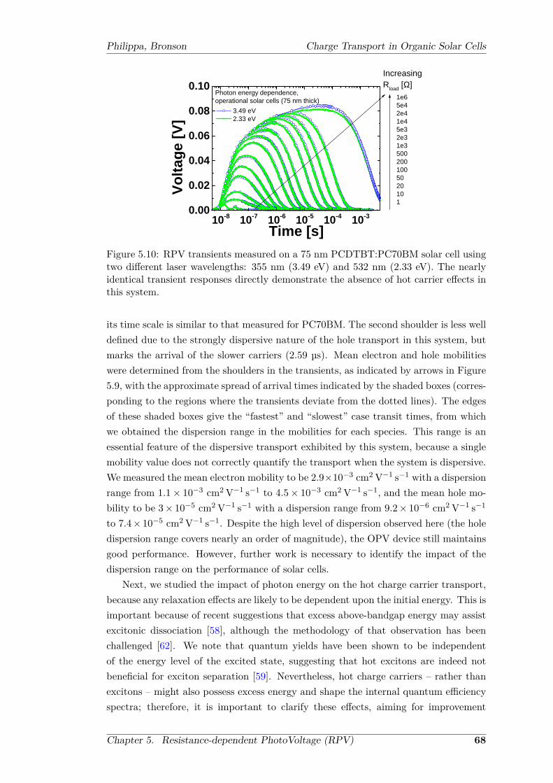
Philippa, Bronson Charge Transport in Organic Solar Cells
10-8 10-7 10-6 10-5 10-4 10-30.00
0.02
0.04
0.06
0.08
0.10
3.49 eV 2.33 eV
1e65e42e41e45e32e31e35002001005020101
Vo
ltag
e [V
]
Time [s]
IncreasingR
load [Ω]
Photon energy dependence,operational solar cells (75 nm thick)
Figure 5.10: RPV transients measured on a 75 nm PCDTBT:PC70BM solar cell usingtwo different laser wavelengths: 355 nm (3.49 eV) and 532 nm (2.33 eV). The nearlyidentical transient responses directly demonstrate the absence of hot carrier effects inthis system.
its time scale is similar to that measured for PC70BM. The second shoulder is less welldefined due to the strongly dispersive nature of the hole transport in this system, butmarks the arrival of the slower carriers (2.59 µs). Mean electron and hole mobilitieswere determined from the shoulders in the transients, as indicated by arrows in Figure5.9, with the approximate spread of arrival times indicated by the shaded boxes (corres-ponding to the regions where the transients deviate from the dotted lines). The edgesof these shaded boxes give the “fastest” and “slowest” case transit times, from whichwe obtained the dispersion range in the mobilities for each species. This range is anessential feature of the dispersive transport exhibited by this system, because a singlemobility value does not correctly quantify the transport when the system is dispersive.We measured the mean electron mobility to be 2.9×10⁻³ cm2 V−1 s−1 with a dispersionrange from 1.1× 10⁻³ cm2 V−1 s−1 to 4.5× 10⁻³ cm2 V−1 s−1, and the mean hole mo-bility to be 3× 10⁻⁵ cm2 V−1 s−1 with a dispersion range from 9.2× 10⁻⁶ cm2 V−1 s−1
to 7.4× 10⁻⁵ cm2 V−1 s−1. Despite the high level of dispersion observed here (the holedispersion range covers nearly an order of magnitude), the OPV device still maintainsgood performance. However, further work is necessary to identify the impact of thedispersion range on the performance of solar cells.
Next, we studied the impact of photon energy on the hot charge carrier transport,because any relaxation effects are likely to be dependent upon the initial energy. This isimportant because of recent suggestions that excess above-bandgap energy may assistexcitonic dissociation [58], although the methodology of that observation has beenchallenged [62]. We note that quantum yields have been shown to be independentof the energy level of the excited state, suggesting that hot excitons are indeed notbeneficial for exciton separation [59]. Nevertheless, hot charge carriers – rather thanexcitons – might also possess excess energy and shape the internal quantum efficiencyspectra; therefore, it is important to clarify these effects, aiming for improvement
Chapter 5. Resistance-dependent PhotoVoltage (RPV) 68

Philippa, Bronson Charge Transport in Organic Solar Cells
in the charge extraction of typical low mobility organic materials. In the past theabsence of hot charge carrier effects has been observed indirectly [238]. Numericalsimulations predict that RPV is independent of optical interference effects (Figures5.3 and 5.4), allowing direct and unambiguous measurement of any hot charge carriereffects that may be present. RPV transients were measured at two different photonenergies, 3.49 eV (355 nm) and 2.33 eV (532 nm). The results are plotted in Figure5.10, showing nearly identical transients resulting from laser excitation at the twodifferent wavelengths. The photon energy independent mobility suggests that excessenergy plays a minimal role in dispersive transport, since carrier thermalization (if itis present) must happen in time scales much shorter than the transit time.
To further confirm that the dispersion in hot carrier mobilities is not caused by thethermalization of carriers, we studied the electric field and film thickness dependence.Longer transit times should allow more time for thermalization, thus influencing theresult if the dispersion is due to carrier relaxation. The results are shown in Figure5.11. The mobilities and dispersion ranges are completely independent of electric fieldand photon energy [Figure 5.11 (a)], suggesting that trapping mechanisms are moresignificant than relaxation mechanisms. The lack of electric field dependence is incontrast with the Poole-Frenkel dependence reported in pristine PCDTBT [239]. Thisis an unexpected result, because in disordered organic systems significant electric fielddependence is typically observed, even at relatively low values of electric fields [239],which is thought to originate from hopping-type charge transport. Further studiesof the temperature dependence, and measurements on other systems, have to be per-formed in order to clarify the origin of this observation. Additionally, we observe thatthe mean mobilities and dispersion ranges are nearly independent of the film thick-ness [Figure 5.11 (b)]. We attribute the small changes in mobility to device-to-devicevariations that result from the fabrication process. The thickness independence of themean mobilities and dispersion ranges further support the claim that the dispersionis caused by traps instead of relaxation. A charge carrier density dependence in themobility even at low concentrations has been observed in P3HT:PCBM blends [73],and we note that a concentration dependence might cause dispersion as carriers gradu-ally become trapped and the density decreases. We do not exclude the possibility of adensity dependence here. However, in our measurements, increasing thickness corres-ponds to lower densities because the amount of photogenerated charge was always lessthan CU , which is inversely proportional to thickness. Consequently, the thicknessindependence in the mobility implies that there is negligible density dependence at theconcentrations probed here.
Further measurements were also performed on solar cells made with PTB7 blends.Typical transients are shown in Figure 5.12. Only a single transit time is visible, whichwe attribute to the fact that charge transport is more balanced in PTB7 blends than inPCDTBT blends. Nevertheless, the electric field and thickness dependencies show thesame conclusions as the PCDTBT blends: the mean mobility and dispersion rangesare independent of both of these parameters (Figure 5.13). Consequently, the same
Chapter 5. Resistance-dependent PhotoVoltage (RPV) 69

Philippa, Bronson Charge Transport in Organic Solar Cells
5.0x10⁴
1.0x10⁵
1.5x10⁵
2.0x10⁵
10-5
10-4
10-3
10-2
270 nm, 2.33 eV
270 nm, 2.33 eV
75 nm, 3.49 eV75 nm, 2.33 eV
75 nm, 3.49 eV
75 nm, 2.33 eVHoles
Electrons
Me
an
mo
bili
ty[c
m2/V
s]
Electric field [V/cm](a)
0 100 200 300 400
10-5
10-4
10-3
10-2
Holes
Electrons
Me
an
mo
bili
ty[c
m2/V
s]
Active layer thickness [nm](b)
Figure 5.11: Electron and hole mobilities measured in PCDTBT:PC70BM solar cells.The error bars show the dispersion ranges. Carrier mobilities and dispersion rangesare independent of electric field and photon energy [panel (a)], and nearly independentof film thickness [panel (b)], demonstrating that carrier thermalization cannot accountfor the dispersive transport in this system. Consequently, dispersion is caused bytrapping.
Chapter 5. Resistance-dependent PhotoVoltage (RPV) 70

Philippa, Bronson Charge Transport in Organic Solar Cells
Figure 5.12: RPV measurements conducted on PTB7:PC70BM solar cells. Only theslower carrier transit time is visible, possibly because the transport in PTB7 blends ismore balanced than in PCDTBT blends.
arguments apply, and these results appear to be generally applicable and are certainlynot specific to PCDTBT blends.
5.4 DiscussionCharge transport in the studied operational OPV blends is strongly dispersive, asdemonstrated by the decaying time-of-flight photocurrent transients in thick devices(Figure 5.8). These time-of-flight transients were recorded in a regime where driftdominates over diffusion, so the current density is described by j = eE(nµn + pµp),where e is the charge of an electron, µn and µp are the electron and hole mobilities, nand p are the carrier concentrations, and E is the electric field. The observation of adecaying photocurrent density j can be explained by two mechanisms: thermalisation(a time dependent mobility, µ), and/or trapping (a time dependent concentration ofmoving charge carriers, n). These mechanisms are schematically illustrated in Figure5.14, from which it can be seen that either model would result in dispersive photocur-rent transients. We found no evidence of thermalisation-type effects on the timescalescomparable with those involved in charge transport. Figure 5.10 directly demonstratesthat that excess energy of hot carriers has essentially no contribution to mobility ordispersion. In Figure 5.11, we demonstrate that the dispersion range is essentiallyindependent of the applied electric field and changes very little with thickness, overthe ranges that were tested. If thermalisation on transport time scales were the causeof the dispersion, then modifications to the transit time should change the mean mo-bility and/or dispersion range by varying the time available for relaxation. Such a
Chapter 5. Resistance-dependent PhotoVoltage (RPV) 71

Philippa, Bronson Charge Transport in Organic Solar Cells
5.0x10⁴ 1.0x10⁵ 1.5x10⁵ 2.0x10⁵
10-4
10-3
Holes
Mea
n m
obili
ty [c
m2 /V
s]
Electric field [V/cm]
(a)
200 400 600
10-4
10-3 Holes
Mea
n m
obili
ty [c
m2 /V
s]
Active layer thickness [nm]
(b)
Figure 5.13: Mobilities measured in PTB7:PC70BM solar cells, as a function of (a)electric field and (b) film thickness. The mobilities are independent of electric fieldand thickness, as observed above for the PCDTBT blends, suggesting that carrierthermalisation is not the cause of the dispersion in this system.
variation was not observed, and hence we exclude thermalisation as the mechanism ofthe dispersive transport. Any relaxation processes must be much faster than chargetransport, so that the distance covered by charges as they relax is insignificant com-pared with the film thickness, and hence the relaxation has negligible contribution tothe overall dispersion.
With relaxation excluded, the only remaining mechanism is a reduction in theconcentration of moving carriers, therefore, we conclude that trapping is the primarycause of the dispersion in these systems. This challenges the widely-used model ofhot carrier relaxation within the density of states. Consequently, dispersive transportpotentially impacts on the many different devices that employ films made from dis-ordered semiconductors, including those that operate in the dark or at steady-stateconditions.
We cannot exclude the possibility that excess photon energy is not transferred tothe charge carrier at all, i.e. that it is dissipated earlier in the photogeneration pro-cess. Nevertheless, the central conclusion that thermalisation effects are insignificant
Chapter 5. Resistance-dependent PhotoVoltage (RPV) 72

Philippa, Bronson Charge Transport in Organic Solar Cells
Energy
Position
(a) Thermalisation
Energy
Position
(b) Trapping
Mobility decreases as carriers relax
within the density of states. The length
of the arrow indicates the mobility.
Mobility is constant, but carriers are
progressively lost to trap states
Trap
states
Figure 5.14: . Schematic illustration of the two pathways to dispersive transport. (a)Thermalisation causes the mobility to decrease with time, whereas (b) trapping causesthe loss of carrier density. We have shown here that the latter case (trapping) is thedominant effect in the studied solar cells.
is supported by the observation that the mobility is independent of the transit time(Figure 5.11). Even if hot carriers are not formed by high energy photons, dispersivetransport must be caused by trapping rather than energetic relaxation.
5.5 ConclusionElectron and hole mobilities and their dispersion ranges were measured simultaneouslyusing the RPV technique in a high efficiency narrow optical gap polymer/fullerenesystem (PCDTBT:PC70BM). We found that the transport of electrons and holes areboth strongly dispersive in these thin, efficient solar cells. We introduced the dispersionrange as a parameter to quantify charge transport, since a single mobility value isinsufficient to properly characterize a dispersive material.
We directly observed the absence of “hot carrier” effects on time scales relevantto charge extraction, and furthermore found that the dispersion is caused by trappingrather than thermal relaxation. We have found that the widely-used model of hotcarrier relaxation within a density of states is not the dominant process causing thedispersion in the studied solar cells. Furthermore, in contrast with the Poole-Frenkeldependence previously reported in pristine PCDTBT and other disordered systems,the studied solar cell blends exhibit an unexpected negligible electric field dependence.While further work is needed to clarify this observation, electric field independence
Chapter 5. Resistance-dependent PhotoVoltage (RPV) 73

Philippa, Bronson Charge Transport in Organic Solar Cells
may assist in maintaining a good fill factor by keeping the mobility higher near themaximum power point. The absence of hot carrier effects and an electric field in-dependent mobility were also observed in PTB7:PC70BM solar cells, suggesting thatthese conclusions may be more generally applicable.
This work signifies the importance of localized trap states as opposed to thermal-ization and hot carrier effects in efficient polymer-based solar cells. Since dispersionarises from trapping, it is also important for other types of devices, such as organicfield effect transistors and diodes. Trap states are relevant whether the carriers wereinjected or photogenerated, and whether the device is in transient or equilibrium con-ditions. Our results suggest that further scientific research should be directed towardsreducing the density of trap states rather that utilizing above-bandgap energy for im-proving electronic device performance.
Chapter 5. Resistance-dependent PhotoVoltage (RPV) 74

6High Intensity RPV (HI-RPV)
This chapter contains material that has been published in the following journal article:[2] Bronson Philippa, Martin Stolterfoht, Ronald D. White, Marrapan Velusamy,
Paul L. Burn, Paul Meredith, and Almantas Pivrikas. Molecular weight dependentbimolecular recombination in organic solar cells. The Journal of Chemical Physics,141, 054903 (2014). doi:10.1063/1.4891369.
The low molecular weight polymer studied here was fabricated by Marrapan Velusamy.Solar cells were manufactured and measured by Martin Stolterfoht, Anton Bavdek, andAlmantas Pivrikas. The analysis of this data that is presented here was performed byme. All other work described in this chapter is my own.
6.1 IntroductionThe previous chapter presented results of applying the RPV technique at low lightintensities in order to study mobility. It was shown that RPV was a robust tool,and that it is applicable to operational solar cell devices. In this chapter, the RPVtechnique is extended to high light intensities in order to probe carrier recombination.Recombination is important because it is one of the key loss mechanisms in organicbulk heterojunction solar cells, especially those with thicker junctions or those madefrom materials which do not possess a sufficiently high carrier mobility [12,82,240].
Recombination coefficients are commonly compared with the prediction of Langevin[12,89,92], which is βL = e (µp + µn) /ϵϵ0, where e is the charge of an electron, µp (µn)is the mobility of holes (electrons), and ϵϵ0 is the dielectric permittivity. A suppressed,non-Langevin recombination coefficient (with β < βL) has been reported in organicphotovoltaic blends that exhibit high performance [94, 95, 103, 241, 242]. Suppressed
75

Philippa, Bronson Charge Transport in Organic Solar Cells
recombination is desirable to ensure efficient charge extraction. The reduction factorβ/βL is a useful “figure of merit” for screening candidate photovoltaic blends to rapidlyidentify those which are likely to be highly performing [89].
A variety of techniques are available to study recombination dynamics. Techniquesthat operate on fully operational devices (i.e. those without blocking layers or othermodifications [104]) include transient photovoltage (TPV) [147, 149], photogeneratedcharge extraction by linearly increasing voltage (photo-CELIV) [128, 129], and time-of-flight (TOF) [124,125].
TPV studies often show an apparent reaction order higher than the expected valueof two [150]. It has been suggested that this is due to a concentration dependence in therecombination coefficient [243], recombination through trap states [244], or the spatialseparation of the carriers under open circuit conditions [150]. The spatial separation atopen-circuit conditions can be reduced by studying the solar cell nearer to short-circuitconditions [20], as in the photo-CELIV or TOF experiments.
Photo-CELIV can be used to study charge carrier mobility and also the bimolecularrecombination coefficient [7,245–249]. The recombination coefficient can be estimatedfrom the maximum extraction current in the photo-CELIV transient [100, 133]. How-ever, this transient is influenced by experimental factors that are not fully accountedfor in the theory, such as the spatial distribution of light absorption [133], the circuitresistance [21], and the voltage slope [131]. Additionally, premature escape of chargefrom the film [250] contributes to the charge redistribution during the delay time [145],which results in a false position of the extraction maximum and makes the measure-ment unreliable. While some attention has been directed to minimizing this issue [72],a full compensation of carrier redistribution is impossible due to Fermi level pinning,an inhomogeneous electric field inside the film and strong diffusion near the electrodewhere carriers are photogenerated.
Another well known technique to characterise recombination is high intensity time-of-flight (TOF) [75,112,113]. The recombination coefficient can be estimated from theamount of charge extracted during a TOF experiment [89,102,223]. However, the ex-ternal circuit resistance influences the extracted charge [95], making the measurementunreliable due to its dependence on the experimental conditions. Previous works haveneglected the impact of the RC circuit [89]. Here, we resolve this issue by extendingthe previous work to achieve more reliable experimental results.
In this chapter, we study recombination in the benchmark organic photovoltaicsystem PCDTBT:PC70BM (see the experimental section for details of the materials).We quantify the recombination in this system, and compare solar cells made withlow molecular weight PCDTBT to those made with high molecular weight PCDTBT.Our recombination study will be conducted using a variant of time-of-flight that wecall High Intensity Resistance dependent PhotoVoltage (HI-RPV). An exact analyticsolution of the relevant differential equations is not known, so we apply numericalsimulations to show the applicability of the technique to a variety of experimental
Chapter 6. High Intensity RPV (HI-RPV) 76
Philippa, Bronson Charge Transport in Organic Solar Cells
conditions. After demonstrating the generality of the technique, we go on to apply itto operational bulk heterojunction solar cells.
Our simulations take an effective medium approach to model device-scale beha-viour, an approach which is commonly used for organic solar cell simulation [20–22,144, 251, 252]. We consider the situation where the films are not doped and there isno film charging due to deep traps whose release times are longer than the transittime. These assumptions are typically met in high efficiency devices. The details ofour numerical solver were described in Chapter 3.
6.2 Experimental SetupThe experimental setup is shown in Figure 6.1. Similarly with time-of-flight, chargesare photogenerated using a high intensity laser, and the voltage across the load resistoris measured with an oscilloscope. However, in contrast with traditional time-of-flight,the measurement is repeated many times across a wide range of load resistances. Fur-thermore, volume photogeneration is desirable, and consequently operational thin-filmsolar cells can be studied.
The experiment begins with the photogeneration of a large quantity (≫ CU) ofcharge carriers using an intense laser pulse. These carriers induce a photocurrent thatcharges the electrodes, which act as capacitive plates. The electrodes rapidly acquirea charge of CU , where C is the capacitance and U is the solar cell’s built-in field(or the applied voltage). Next, two processes occur simultaneously. The first is therecombination of the photogenerated charges, and the second is the discharge of thecapacitor through the external RC circuit. If the RC time is large, then the photo-carriers will completely recombine before the capacitor can discharge, and the totalextracted charge will be limited to CU . Conversely, if the RC time is small, then thecapacitor will discharge before the carriers completely recombine, more photocurrentwill flow, and the extracted charge will exceed CU . In the intermediate regime, thereis an interplay between the bimolecular lifetime and the RC time. We exploit thisrelationship in order to quantify the carrier recombination.
6.3 Device Thickness and Light Absorption ProfileIt has been shown in the past that the light absorption profile strongly affects CELIVtransients [133], so it is important to clarify the impact that the light absorption hason HI-RPV. We apply the Beer-Lambert law to represent the photogeneration profile,
n0 = p0 = Lαe−αx, (6.1)
where n0 (p0) is the initial concentration of electrons (holes), L is the light intensity inphotons per unit area, α is the absorption coefficient at the laser wavelength, and x is
Chapter 6. High Intensity RPV (HI-RPV) 77

Philippa, Bronson Charge Transport in Organic Solar Cells
OscilloscopeRload
+-
DCVoltageSupply
High intensitylaser pulse
Transparentelectrode
Semiconductorblend
Electrode
Record currenttransient using
the oscilloscope
Integrate withrespect to timeto obtain the
extracted charge
Vary loadresistance
Calculate thebimolecular
recombinationcoefficient from
the extractedcharge
Figure 6.1: Circuit schematic for the High Intensity Resistance dependent Photo-Voltage (HI-RPV) experiment. Current transients are recorded across a range of loadresistances, and then integrated to obtain the extracted charge, Qe. The variation inthe extracted charge with resistance is used to quantify the recombination processesand determine the bimolecular recombination coefficient. If the device under test isan operational solar cell, then the DC voltage supply is optional and the experimentcan be done under the solar cell’s built-in field.
the spatial coordinate. Normalising the absorption coefficient α to the film thicknessd, the shape of the initial distribution is described by the dimensionless quantity αd.
We performed numerical simulations at varying values of αd and for varying lightintensities. The light intensity is represented by the quantity of photogeneratedcharge carriers Qph = L
(1− e−αd
), which is the integral of Eq. (6.1) over the
device. We selected a fixed circuit resistance, RC/ttr(sum) = 0.05, where R is theresistance of the circuit external to the device, C is the device capacitance, andttr(sum) ≡ d2 (µp + µn)
−1 U−1 is an effective transit time calculated from the sum ofcarrier mobilities crossing a film of thickness d under a voltage U . The use of µp + µn
in the normalisation scale will be justified below. The bimolecular recombination wasgiven by the Langevin rate (β/βL = 1).
The light intensity dependence in the amount of extracted charge is plotted inFigure 6.2. The simulations were conducted with equal electron and hole mobilities;however, the results are essentially unchanged if the mobilities are not equal (as shownin Figure 6.3). We observe that the extracted charge Qe/CU becomes essentiallyindependent of αd when αd is less than 1. The inset of Figure 6.2 shows the αd
dependence at high light intensity, demonstrating that Qe/CU is essentially insensitive
Chapter 6. High Intensity RPV (HI-RPV) 78

Philippa, Bronson Charge Transport in Organic Solar Cells
10-2
10-1
100
101
102
103
104
105
0.01
0.1
1
Extr
acte
d c
harg
e,
Qe /
CU
Photogenerated carriers, Qph / CU
d = 0.1
d = 1
d = 3
d = 10
d = 30
d = 100
Decreasing film thickness
Langevin recombination; Equal electron & hole mobilities
RC / ttr(sum) = 0.05
0.01 0.1 1 10 100 10001.0
1.5
2.0
2.5
3.0
Qe /
CU
d
Figure 6.2: The impact of the film thickness and light absorption profile on the extrac-ted charge. The film thickness is incorporated within the absorption-thickness productαd (where α is the absorption coefficient and d the thickness). The inset shows the αddependence in the region indicated by the thin grey box (Qph/CU = 104), and demon-strates that the extracted charge is independent of the initial carrier distribution forthin films (αd < 1). The extracted charge readily saturates with high light intensity.This graph shows that a general theory for thin film devices can be developed, withoutdetailed optical modelling, and without regard for the precise quantity of photogener-ated carriers in the saturation regime.
to the initial carrier spatial distribution, in the case of volume generation. For example,in the case of αd = 3 (see Figure 6.2), the light intensity at the back of the deviceis approximately 5% of the light intensity at the front of the device. Such a stronginhomogeneity in the spatial distribution does not meaningfully affect the extractedcharge.
Physically, the insensitivity to the initial spatial distribution is caused by bimolecu-lar recombination. The bimolecular recombination process will be more rapid in re-gions of higher light intensity, and slower in regions of lower light intensity. This will,in effect, “smooth” the carrier distribution across the device, erasing the initial spa-tial distribution. More precisely, the carrier concentration at early times is given byn(t) =
(n−10 + βt
)−1, where n0 is the initial carrier concentration [118]. In the limit ofvery large n0, the dependence on the initial condition vanishes [n(t) ≈ (βt)−1]. Thisexplains why the absorption profile is irrelevant at high light intensities.
In summary, to first order, detailed optical modelling to account for exact carrierdistribution in operational solar cells is not necessary, since the precise spatial dis-tribution of carriers is rapidly erased by bimolecular recombination. Therefore, theHI-RPV technique can be applied to thin film devices (αd ≤ 1) without concern foroptical interference.
Since the technique is insensitive to the light absorption profile, we will removeαd from the set of parameters being tested, and approximate the initial condition by
Chapter 6. High Intensity RPV (HI-RPV) 79

Philippa, Bronson Charge Transport in Organic Solar Cells
10-1 100 101 102 103 104 1050.1
1
Extra
cted
cha
rge,
Qe
/ CU
Photogenerated carriers, Qph / CU
ttr(sum) = d2 ( p + n)-1 U-1
ttr(sum) is the transit timecalculated from the sumof mobilities.
RC / ttr (sum) = 0.01 RC / ttr (sum) = 0.1 RC / ttr (sum) = 1 RC / ttr (sum) = 10 RC / ttr (sum) = 100
Filled symbols: faster / slower = 1Open symbols: faster / slower = 100
Qe(sat) / CUUniform generation (valid for d < 1)Langevin recombination
Figure 6.3: The impact of the circuit resistance on the extracted charge from simu-lated resistance dependent photovoltage experiments. Filled symbols with lines showbalanced mobilities (µfaster/µslower = 1); open symbols without lines show stronglyunbalanced mobilities (µfaster/µslower = 100). The two are very similar, because thenormalisation scale for the circuit RC time minimises the effect of the mobility ratio.The saturation value Qe(sat)/CU depends almost entirely upon the normalised resist-ance. These results demonstrate that the load resistance needs to be accounted for tocorrectly measure the recombination coefficient.
perfectly uniform carrier generation. All subsequent numerical calculations are per-formed with this simplified uniform initial condition, rather than the Beer-Lambertlaw. Using this approximation, the simulation parameters are reduced to light intens-ity (expressed as Qph/CU), recombination coefficient (expressed as β/βL), mobilityratio µfaster/µslower, and the circuit resistance (expressed as RC/ttr(sum)). The circuitresistance, which we will address next, is a crucial parameter that may have beenoverlooked in the past [95].
6.4 Circuit ResistanceIn a HI-RPV experiment, the circuit resistance is varied over many orders of magnitudein order to observe the dynamical interaction between the known circuit RC time andthe unknown bimolecular lifetime.
We examined the impact of the circuit resistance using our simulations, as shownin Figure 6.3. Importantly, we observe that more charge can be extracted at lowerresistances. A smaller resistance allows the charge extraction to complete in a shortertime, so that less recombination occurs, and the overall extracted charge is higher.
The faster carrier mobility is normalised out of the simulation by the system of units(as described in Chapter 3). However, it is necessary to specify the ratio of carriermobilities µfaster/µslower. To confirm that variation in this ratio will not interfere withthe measurement, Figure 6.3 shows the case of balanced mobilities (µfaster/µslower = 1)
Chapter 6. High Intensity RPV (HI-RPV) 80

Philippa, Bronson Charge Transport in Organic Solar Cells
10-5
10-4
10-3
10-2
10-1
100
101
102
103
104
0
2
4
6
8
10
12
µfaster
/ µslower
= 1
µfaster
/ µslower
= 10
µfaster
/ µslower
= 100
Equation (3)
Sa
tura
ted
extr
acte
d c
ha
rge
, Q
e(s
at) /
CU
Normalised circuit resistance, RC / ttr(sum)
High light intensity (Qe saturated)
Langevin recombination
Uniform photogeneration (valid for d < 1)
ttr(sum) is the transit time
calculated from the sum
of mobilities.
ttr(sum) = d2 (µp + µn)
-1 U
-1
Figure 6.4: Simulations of the impact of load resistance on the extracted charge fromthin film devices with Langevin recombination at varying mobility ratios. Points arecalculated from simulations at high light intensity (Qph/CU = 106, although the pre-cise value is unimportant because of the saturation in the extracted charge Qe, asshown in Figure 6.3). The ratio of carrier mobilities does not affect the extractedcharge, so HI-RPV measurements can be applied equally to systems with balancedmobilities and systems with strongly unbalanced mobilities.
with filled symbols and lines and strongly unbalanced mobilities (µfaster/µslower = 100)with open symbols and no lines. This covers a wide range of mobility ratios to examinethe variation that might be expected to occur in practice. The two cases (balanced mo-bilities and strongly unbalanced mobilities) are essentially indistinguishable, as shownin Figure 6.3. We explain this insensitivity as follows. The amount of extracted chargeQe is primarily controlled by the recombination. The Langevin recombination rate isproportional to the sum of carrier mobilities. The relevant time scale for this processis ttr(sum) ≡ d2/ (µp + µn)U .
Figure 6.3 shows that the extracted charge saturates at high light intensities toa value that we call Qe(sat)/CU , as indicated by the arrows. Therefore, if the HI-RPV experiment is operated in this saturation regime, the amount of extracted chargedoes not depend on the laser power which is applied. The extracted charge is alsoindependent of the carrier mobility ratio (Figure 6.3) and the light absorption profile(Figure 6.2). Consequently, the only parameters remaining to be quantified are thecircuit resistance and the bimolecular recombination coefficient.
The impact of the circuit resistance is shown in Figure 6.4. If the normalisedresistance is small, the extracted charge Qe(sat) can exceed the charge on the electrodesCU by an order of magnitude or more, even in the presence of Langevin recombination.The TOF experiment under these circumstances is therefore misleading, especially ifcomparing two systems with different values of the normalised resistance, RC/ttr(sum).We resolve this problem by introducing the HI-RPV technique. We firstly develop
Chapter 6. High Intensity RPV (HI-RPV) 81

Philippa, Bronson Charge Transport in Organic Solar Cells
predictions for Langevin systems, and then in the following section extend this to thegeneral case.
Figure 6.4 shows a single universal curve that all Langevin systems should obey.We developed an empirical equation to describe this curve by arbitrarily choosing anappropriate functional form that would give a logarithmic dependence at small R (asshown in Figure 6.4), and would saturate to 1 at large R (as also shown in Figure 6.4),
Qe(sat)CU
= 1 + p1 log[1 + p2
(ttr(sum)RC
)p3]. (6.2)
We used non-linear least squares regression to calculate the coefficients pi from thesimulation results in Figure 6.4. The result is:
Qe(sat)CU
= 1 + 1.8 log[1 + 0.63
(ttr(sum)RC
)0.55], (6.3)
which is valid for Langevin recombination and thin films. Equation (6.3) is plottedagainst the simulation results in Figure 6.4, demonstrating excellent agreement.
The purpose of Eq. (6.3) is to determine the type of recombination present in a thinfilm device; for example, one could plot this equation alongside measured data in orderto determine whether the recombination is of the Langevin type. This is important,since recombination orders higher than two have been experimentally observed [150],and it is necessary to identify the type of recombination dynamics that might applyto the system being studied. A plot of extracted charge versus resistance (Figure 6.4)will follow the form of Eq. (6.3) if Langevin recombination is dominant. In contrast,if there is a higher order of recombination, then the carrier concentration will decayaccording to a different time dependence, and the functional form of the extractedcharge versus resistance will change. If the recombination is stronger than Langevin,the experimental data will lie below the line. On the other hand, if the dominant formof recombination is slower than Langevin, then less recombination will occur and theexperimental data will lie above the line.
We will show below that our experimental data can be described by a bimolecularrecombination process with a Langevin reduction prefactor. We do not exclude thepossibility of higher-order effects such as a concentration-dependent recombinationcoefficient [243], but these are not necessary to explain our data. Therefore, in thefollowing section, we extend our theory to systems with suppressed (non-Langevin)recombination of purely second order.
6.5 Bimolecular Recombination CoefficientIn order to develop a tool for convenient experimental quantification of the recom-bination coefficient (β/βL), we applied numerical simulations to predict the amountof extracted charge as a function of β/βL. These simulations are plotted in Figure
Chapter 6. High Intensity RPV (HI-RPV) 82

Philippa, Bronson Charge Transport in Organic Solar Cells
10-4
10-3
10-2
10-1
100
101
102
103
104
100
101
102
103
104
Filled symbols: f /
s = 1
/L = 0.001
/L = 0.003
/L = 0.01
/L = 0.03
/L = 0.1
/L = 0.3
/L = 1
Open symbols: f /
s = 10
/L = 0.01
/L = 1
Sa
tura
ted
extr
acte
d c
ha
rge
, Q
e(s
at) /
CU
Normalised circuit resistance, RC / ttr(sum)
Uniform photogeneration (valid for d < 1)
High light intensity (saturated regime)
Points are from simulation
Lines are from Eq. (2)
Figure 6.5: Numerically predicted extracted charge as a function of load resistance inHigh Intensity Resistance dependent PhotoVoltage (HI-RPV) experiments for differentrecombination coefficients β/βL. The extracted charge shown in this figure is calculatedat the highest light intensities where the extracted charge saturates, as shown in Fig.6.2. The points are from simulations, whereas the lines are Eq. (6.2) evaluated foreach respective value of β/βL. This graph presents numerical predictions to be usedwhen measuring the recombination coefficient β/βL experimentally from HI-RPV insystems without deep traps.
6.5. As expected, the amount of extracted charge increases dramatically in the pres-ence of non-Langevin recombination. To confirm that our technique remains valid, wechecked that non-Langevin devices also exhibit saturation at high light intensity, andthat the extracted charge is independent of the optical absorption profile for thin films(αd < 1). We found that systems with strongly suppressed recombination (β ≪ βL)exhibit a stronger dependence on the mobility ratio than Langevin systems. The moreunbalanced the mobilities, the less charge can be extracted. A representative example(µfaster/µslower = 10) is plotted in Figure 6.5 with open symbols.
We are now ready to specify how the HI-RPV technique can be applied. Therecombination coefficient can be determined by comparing measurements of the ex-tracted charge against the simulation results in Figure 6.5. This approach is validfor any thin film (αd < 1) device. Importantly, this technique is not hindered by theRC-dependence that affects traditional high intensity TOF [89,95], because the impactof the RC time constant on the extracted charge is accounted for on the horizontalaxis of Figure 6.5. However, for accurate measurements, it is necessary to reach theregime where RC/ttr(sum) ≪ 1. This may not be possible in extremely high mobilitymaterials, especially when the series resistances are included in R. Ideally, R shouldbe varied over many orders of magnitude.
As an alternative to visual inspection of the graph, we can also specify an empiricalequation that describes the data in Figure 6.5. We started with the general functionalform [Eq. (6.2)] and applied a procedure similar to that described earlier for the
Chapter 6. High Intensity RPV (HI-RPV) 83

Philippa, Bronson Charge Transport in Organic Solar Cells
Langevin case. We performed simulations across a physically realistic parameter spacein both RC/ttr(sum) and β/βL. The simulations were performed with balanced mobil-ities, because that corresponds to the maximum extracted charge. With least squaresregression, we found the parameters pi as a function of β/βL. Finally, we parametrisedthe pi values as follows, choosing an arbitrary functional form that best described thedata:
p1 = 1.829
(β
βL+ 0.0159
√β
βL
)−1
(6.4)
p2 = 0.63
(β
βL
)0.407
(6.5)
p3 = 0.55
(β
βL
)0.0203
. (6.6)
These functional forms were found to obtain the best fit to the simulated results.Figure 6.5 shows the simulation results compared with Eq. (6.2) with the para-
meters (6.4)-(6.6). A good agreement is demonstrated for balanced mobilities; if themobilities are unbalanced then Eq. (6.2) will slightly overestimate the extracted charge.
These equations are a convenient tool to analyse experimental data. For example,to determine the recombination coefficients for the data presented below, we set up aspreadsheet table to compare the model with experimental data and thereby estimatethe bimolecular recombination coefficient.
In order to confirm the validity of the newly presented HI-RPV technique, wehave compared its results in various systems with other techniques including photo-CELIV [129], double injection transients [253] and plasma extraction [254]. The resultsare in agreement, given the limitations of each technique. These limitations must becarefully considered when comparing measurements, which is why we have developedthe present HI-RPV approach.
6.6 Experimental MeasurementsWe manufactured bulk heterojunction organic solar cells with the donor:acceptor blendpoly[N-9”-hepta-decanyl-2,7-carbazole-alt-5,5-(4’,7’-di-2-thienyl-2’,1’,3’-benzothiadiazole)](PCDTBT) and [6,6]-phenyl-C71-butyric acid methyl ester (PC70BM). This blend,PCDTBT:PC70BM, has previously been reported to exhibit near to Langevin recom-bination [75]. Two sources of PCDTBT were used. A low molecular weight batch(Mn = 4.3 kDa, Mw = 12.1 kDa, PDI = 2.8, dissolved in 1,2,4-trichlorobenzene at 140C) was synthesized in our laboratory following the Suzuki cross-coupling protocolspreviously described [255]. A high molecular weight batch (Mn = 22.7 kDa, Mw =122.2 kDa, PDI = 5.4) was purchased from the SJPC Group.
The fabrication of the solar cells followed a previously described procedure [6]. 15Ω/sq. Indium Tin Oxide (ITO) coated glass substrates patterned by photolithography(Kintec) were cleaned by sonicating in sequence with alconox (detergent), de-ionised
Chapter 6. High Intensity RPV (HI-RPV) 84

Philippa, Bronson Charge Transport in Organic Solar Cells
10-1
100
101
102
103
104
105
0
1
2
3
4
Material: PCDTBT:PC70BM
90 nm, high MW
75 nm, high MW
Eq. (2) with β/βL = 0.07
130 nm, low MW
46 nm, low MW
Eq. (2) with β/βL = 1
Satu
rate
d e
xtr
acte
d c
harg
e,
Qe
(sa
t) /
CU
Normalised circuit resistance, Rtotal
C / ttr(sum)
Langevin;
low molecular
weight
Non-Langevin;
high molecular
weight
ttr(sum) is the transit time calculated from the sum of mobilities.
ttr(sum) = d2 (µp + µn)
-1 U
-1 = ttr(faster)(1 + ttr(faster)/ttr(slower))
-1
Figure 6.6: Experimentally measured extracted charge as a function of circuit resist-ance obtained using the HI-RPV technique. Films made with the low molecular weightpolymer exhibit Langevin recombination, whereas films containing the high molecularweight polymer exhibit suppressed non-Langevin recombination. Non-Langevin recom-bination is beneficial to solar cell performance, indicating the importance of materialquality in device fabrication.
water, acetone, and iso-propanol for 10 minutes. The cleaned substrates were coatedwith a 20 nm layer of poly(3,4-ethylenedioxythiophene):poly(styrene sulfonate) (PE-DOT:PSS) by spin casting at 5000 rpm for 60 sec. The PEDOT:PSS layer was bakedfor 10 minutes at 170 C. A solution of PCDTBT and commercially purchased PC70BM(Nano-C) with a mass ratio of 1:4 was prepared at a total concentration of 20 mg/mLin anhydrous 1,2-dichlorobenzene. This solution was deposited by spin coating on topof the PEDOT:PSS layer after filtration. Two substrates were prepared from the lowmolecular weight batch with active layer thicknesses of 46 nm and 130 nm, respect-ively. From the high molecular weight batch, two additional substrates were made withactive layer thicknesses of 75 nm and 90 nm. Thicknesses were measured by a VeecoDektak150 profilometer. Slow drying was performed after spin coating by placing thecoated film in a partially opened petri dish for 2 hours. Finally, a 100 nm aluminiumlayer was deposited by thermal evaporation under a 10−6 mbar vacuum. The deviceareas were 0.035 cm2 with three devices per substrate. The low molecular weight ma-terial produces solar cells with power conversion efficiencies (PCE) of approximately4%; whereas optimised solar cells made from the high molecular weight material havePCEs in excess of 6% [256]. Transit times were measured using low light intensity res-istance dependent photovoltage [3]; the mobilities were µlow MW ≈ 8×10⁻⁵ cm2V−1s−1
and µhigh MW ≈ 2×10⁻³ cm2V−1s−1, demonstrating greatly improved charge transportin the latter devices.
HI-RPV measurements were performed using a pulsed third-harmonic Nd:YAGlaser (Quantel Brio) working at a wavelength of 355 nm and pulse duration of 5 ns.
Chapter 6. High Intensity RPV (HI-RPV) 85

Philippa, Bronson Charge Transport in Organic Solar Cells
At 355 nm, the absorption coefficient of this blend [65] is 8×104 cm−1, which gives αdvalues of 0.37 for the thinnest device (46 nm) and 1.0 for the thickest device (130 nm).The laser beam was attenuated using a neutral density filter set. No external voltagewas applied; instead, the transients were driven by the solar cells’ built-in field. Thesignal was recorded by a digital storage oscilloscope (LeCroy Waverunner A6200).
We performed HI-RPV with load resistances in the range from 1 Ω to 1 MΩ. Theresults are plotted in Figure 6.6. This graph demonstrates the application of the HI-RPV technique. It is important to note that the resistance value R on the horizontalaxis is the complete circuit resistance, calculated as the sum of the load resistance andthe solar cell series resistance. The experimental data is plotted together with thepredicted curve from Eq. (6.2) with parameters (6.4)-(6.6). The measured extractedcharge behaves as expected and as predicted by the simulations. The extracted chargedecreases with increasing resistance until it saturates to Qe(sat)/CU = 1. To determ-ine the recombination strength, the coefficient β/βL was adjusted until the predictedcurves matched the experimental data.
Our results indicate that low molecular weight devices exhibit Langevin-type re-combination, while the high molecular weight devices exhibit non-Langevin recom-bination with β/βL ≈ 0.07. Photo-CELIV measurements applied to the same devicesdemonstrated Langevin and non-Langevin recombination, respectively, supporting ourresults. However, photo-CELIV is subject to various limitations, as we discussed inthe Introduction, and so we developed HI-RPV for the detailed study. The strongchange in the recombination strength likely contributes to the improved power con-version efficiency of the high molecular weight blend. It has previously been reportedthat PCDTBT solar cell performance improves with increasing molecular weight [257].Our results indicate that suppressed recombination may be the mechanism behindthis performance trend, and hence the molecular weight is a parameter that shouldbe considered when optimising solar cell performance. There may be further per-formance improvements to be gained by identifying the molecular weight at which therecombination is minimised.
A previous study of recombination in PCDTBT solar cells [75] reported reductionfactors in the range of β/βL = 0.3 to β/βL = 1 depending upon the device thick-ness. Thinner devices were reported to exhibit more strongly reduced recombination.Thickness dependencies cannot be reliably studied using time-of-flight because vari-ations in the thickness influence parameters such as the device capacitance, the RCtime, the transit time, the optical absorption profile, and the amount of extractedcharge. Consequently, with time-of-flight it is difficult to eliminate the dependenceon the experimental parameters. In contrast, HI-RPV accounts for these effects. Wedid not observe any thickness dependence, although the range of thicknesses measuredhere is less than that in the previous study [75].
Further work is necessary in order to clarify the origin of this molecular weightdependence, as well as any dependence on other parameters such as polydispersity,
Chapter 6. High Intensity RPV (HI-RPV) 86
Philippa, Bronson Charge Transport in Organic Solar Cells
impurity density, and conjugation length. The novel HI-RPV technique will be bene-ficial for such future work.
6.7 ConclusionWe studied recombination in the organic photovoltaic system PCDTBT:PC70BM, andobserved that devices made with a higher molecular weight polymer exhibit suppressedrecombination relative to devices made with a lower molecular weight polymer. Ourresults highlight the importance of material quality for fabrication of high efficiencyorganic solar cells. We developed and implemented a theoretical framework for thenovel High Intensity Resistance dependent PhotoVoltage (HI-RPV) technique, whichallows recombination measurements that are independent of the experimental con-ditions, resolving a key weakness of previous time-of-flight based techniques. A keyadvantage of HI-RPV is its insensitivity to the light absorption profile in thin films,making it applicable to operational devices.
Chapter 6. High Intensity RPV (HI-RPV) 87

7Intensity Dependent Photocurrent
(IPC)
This chapter contains material that has been submitted for publication:
• Martin Stolterfoht, Ardalan Armin, Bronson Philippa, Ronald D. White, PaulL. Burn, Paul Meredith, Gytis Juška, and Almantas Pivrikas. Photocarrier driftdistance in organic solar cells and photodetectors. Scientific Reports (submitted).
This chapter contains experimental data that was measured by Martin Stolterfoht, Ar-dalan Armin, and Almantas Pivrikas. Figure 7.9 was prepared by Martin Stolterfoht,and is reproduced here because it provides a validation of my theoretical work. Thediscussion here focusses on the simulation and theoretical aspects of the above paper,which were my contribution.
7.1 IntroductionThe previous chapters reported experimental methods based on photoconduction tran-sients, where current transients are measured after a nanosecond laser excitation. Asolar cell spends the vast majority of its time under steady-state conditions, and someasurements conducted at steady-state would be the most representative of actualoperational conditions. In this chapter, we study steady-state photocurrent. We exam-ine the influence of the carrier mobilities, recombination coefficient, and trapping onthe photocurrent that a solar cell can produce. We show that variation in the light in-tensity can be used to observe the onset of fast bimolecular recombination, and thereby
88

Philippa, Bronson Charge Transport in Organic Solar Cells
present “design rules” for achieving high transport efficiency without bimolecular re-combination.
We will investigate the solar cell’s photocurrent as a function of light intensity.Typically, this would be done under short circuit conditions, but it is also possible toapply a bias to test the device’s response at the maximum power point. We call thismeasurement intensity dependent photocurrent (or IPC). This technique is very com-mon in the literature [73,242,258–260], where it is often used as a test for bimolecularrecombination. Many studies report a power law dependence, i.e. jsc ∼ Lα where jsc isthe short-circuit current, L is the light intensity, and α is the power law slope. A lineardependence (α = 1) is known to indicate the absence of bimolecular recombination,whereas sublinear slopes (α < 1) indicate bimolecular recombination losses [242, 261].If this measurement is taken over a small range of light intensities [259], the true func-tional shape of α may be hidden, and so many orders of magnitude of light intensitiesare needed. Over a large range, one often observes a transition between linear beha-viour at low light intensities, to sublinear behaviour at higher light intensities [242].This indicates a transition from recombination-free to recombination-limited beha-viour. Here, we will systematically examine this effect in order to understand theconditions under which bimolecular recombination is significant and the conditionsunder which it may be avoided or minimised.
7.1.1 Device fabrication and methods
Two different organic solar cell materials were used in this study. The first waspoly[[4,8-bis[(2-ethylhexyl)oxy]benzo[1,2-b:4,5-b’]dithiophene-2,6-diyl][3-fluoro-2-[(2-ethyl-hexyl)carbonyl]thieno[3,4-b]thiophenediyl]]:[6,6]-phenyl-C70-butyric acid methyl ester(PTB7:PC70BM) [262], while the second was poly[N-9”-hepta-decanyl-2,7-carbazole-alt-5,5-(4’,7’-di-2-thienyl-2’,1’,3’-benzothiadiazole)] (PCDTBT):PC70BM [65]. To fab-ricate the devices, the substrates were prepared as described previously [263]. For thePTB7 devices, the active layer solution of PTB7 (purchased from 1-Material, Mw =97.5 kDa, PDI = 2.1) and PC70BM (American Dye Source, Inc., Canada) was blendedin a 1:1.5 ratio by weight in chlorobenzene with 3% 1,8-diiodoctane (DIO) by volume.Solar cells with three different junction thicknesses were prepared by using a total con-centration of 31 mg/cm3 for the 100 nm and 230 nm thick devices and a concentrationof 45 mg/cm3 for the 700 nm thick device. The solutions were spun cast at 2200 rpm,400 rpm and 600 rpm for 120 seconds, respectively. The films were subsequently driedat 70 °C. For the PCDTBT devices, the solution of PCDTBT (SJPC, Canada, Mw= 122 200 g/mol, PDI=5.4) and PC70BM was blended in a 1:4 ratio by weight in1,2-dichlorobenzene. Solar cells with three active layer thicknesses, 75 nm, 230 nmand 850 nm were fabricated by using a total concentration 25 mg/cm3 for the 100nm and 230 nm thick blends respectively, while a concentration of 40 mg/cm3 wasused to fabricate the 850 nm thick film. The solutions were spun cast at 2000 rpm,500 rpm and 500 rpm for 90 seconds, respectively. The active layer thicknesses weremeasured with a DekTak 150 profilometer. All devices were completed by vacuum
Chapter 7. Intensity Dependent Photocurrent (IPC) 89

Philippa, Bronson Charge Transport in Organic Solar Cells
10−5
10−4
10−3
10−2
10−1
100
101
102
103
104
105
10−4
10−3
10−2
10−1
100
101
102
103
104
βL/β = 1
Generation rate (CU/ttr
slower)
Short
circuit c
urr
ent (C
U/t
trslo
we
r )
µf / µ
s = 1000
µf / µ
s = 100
µf / µ
s = 10
µf / µ
s = 1
Figure 7.1: Simulated IPC data for various carrier mobility ratios. There is a universalshape that applies independently of the carrier mobility ratio, allowing general predic-tions to be made. For these simulations, the recombination coefficient was Langevin,i.e. βL/β = 1. Simulation results are shown with points, and the lines are a guide tothe eye.
evaporation of 1.2 nm of samarium followed by 75 nm of aluminum under a 10−6 mbarvacuum. The device areas were 0.2 cm2 for current-voltage curves (JV), IPC and EQEmeasurements, and 3.5 mm2 for RPV measurements (to characterise the mobility andcalculate Isclc). All device fabrication took place within a glove box with < 1 ppmoxygen and water. JV and EQE measurements were also performed inside a glove box.Subsequently the devices were encapsulated for the IPC measurements.
Simulations were conducted using the model described in Chapter 3. Of particularimportance to this work is the normalisation scale that was described in that chapter.Notably, the light intensity is incorporated into the concomitant generation rate offree carriers. In other words, the efficiency of exciton separation is included in thegeneration rate. The objective of this work is to focus on charge transport, and soall the effects of light absorption, exciton separation, etc. are simply lumped togetherinto an overall generation rate. This generation rate will itself be normalised withrespect to CU/tslower
tr , where C is the device’s capacitance, U is the effective voltage(the built-in field plus any applied voltage), and tslower
tr is the transit time of slowercarriers. The chosen charge scale (CU) is a natural choice because it indicates theapproximate threshold at which space charge effects begin to appear. Similarly, thetransport time tslower
tr is a natural time scale because it indicates the amount of timethat a carrier would be expected to remain inside the device. Photocurrent is alsonormalised with respect to the same scale.
7.2 The Universal Functional FormInitially considering the case of Langevin-type recombination, we simulated the IPCexperiment over a very large range of light intensities. The results shown in Figure
Chapter 7. Intensity Dependent Photocurrent (IPC) 90

Philippa, Bronson Charge Transport in Organic Solar Cells
7.1 display two notable features. Firstly, there is a universal functional form, andconsequently variations in any of the parameters in the normalised generation rate(e.g. mobility, dielectric constant, thickness, ...) will simply move along the universalcurve. The second notable feature is that the deviation point separating the linearand sublinear regimes always occurs at the same normalised light intensity, that beingwhen the generation rate of free carriers is equal to CU/tslower
tr .There is much information encoded in the normalised axes. Increasing the light
intensity has the impact of moving right and upward, following the universal shapeof Figure 7.1. A more interesting result is that variations in any of the parameterscontained within CU/tslower
tr would also move along the curve. For example, increasingthe slower-carrier mobility while holding everything else constant moves to the leftbut also down. This is counter-intuitive: an improved mobility results in a lowerphotocurrent! However, a reduction in normalised photocurrent does not necessarilycorrespond to a reduction in actual photocurrent because the normalisation scale alsochanges. The interplay between normalised units and real units provides crucial insightthat endows Figure 7.1 with much predictive power.
According to this simple model, variations in mobility have no impact on the pho-tocurrent if the device remains in the linear regime. Physically, in this regime, thereis negligible recombination, so charge transport is already sufficient to extract chargesbefore they recombine, and improving the mobility provides no further benefit. Adifferent situation arises in the sublinear regime, where an improvement in mobilitywould indeed improve the photocurrent. For example, consider a ten-fold improvementin slower-carrier mobility. The operating point moves one decade to the left in Figure7.1, resulting in approximately a three-fold decrease in normalised current. However,the scaling factor to convert that normalised current back to real units increased by afactor of ten, resulting in a net gain of ∼ 10/3 or approximately 3 times improved pho-tocurrent. It is not just mobility that can be considered in this way, because CU/tslower
tralso contains the dielectric constant, active layer thickness, voltage, etc. This modelallows predictions to be made with respect to any of these parameters.
In the discussion above, we assumed that non-geminate recombination caused thedeviation from linearity, as has been previously reported [242]. To confirm this claim,we replotted the simulation of Figure 7.1 as internal quantum efficiency (IQE) andrecombination losses, as shown in Figure 7.2. It is possible to plot recombinationlosses directly because the simulation allows access to such information that would notbe observable in a real experiment. These results clearly show that the drop in IQE,and hence the sublinear behaviour at higher light intensities, is caused by non-geminaterecombination.
7.3 Non-Langevin RecombinationThe impact of non-Langevin recombination (i.e. βL/β > 1) is to prolong the deviationfrom linearity until higher normalised generation rates, as shown in Figure 7.3. The
Chapter 7. Intensity Dependent Photocurrent (IPC) 91

Philippa, Bronson Charge Transport in Organic Solar Cells
0
50
100(a)
IQE
(%
)
µf / µ
s = 1000
µf / µ
s = 100
µf / µ
s = 10
µf / µ
s = 1
10−4
10−3
10−2
10−1
100
101
102
103
104
105
0
50
100(b)
Generation rate (CU/ttr
slower)
Carr
iers
lost to
non−
gem
inate
recom
bin
ation (
%)
Figure 7.2: (a) Simulated internal quantum efficiency (IQE) as a function of lightintensity for various carrier mobility ratios. The decline in IQE exactly coincides withthe onset of non-geminate recombination as shown in panel (b).
10−2
10−1
100
101
102
103
104
(a)
Short
circuit c
urr
ent (C
U/t
trslo
we
r )
βL / β = 1000
βL / β = 100
βL / β = 10
βL / β = 1
10−2
10−1
100
101
102
103
104
105
20
40
60
80
100(b)
Generation rate (CU/ttr
slower)
IQE
(%
)
Figure 7.3: Simulated IPC data for various recombination coefficients. Panels (a)and (b) are from the same simulations. The impact of non-Langevin recombinationis to allow higher light intensities without losses. It can be seen that the benefit isapproximately proportional to the square root of βL/β.
data are presented in two forms: as intensity-dependent photocurrent (Figure 7.3a)and also as internal quantum efficiency (Figure 7.3b). The advantage of the latter isthat the onset of recombination is more clearly visible.
To make predictions about the amount of recombination that should occur, we de-sire a normalisation scale that will collapse all the data into the same universal curve,as was done above with Figure 7.1. Figure 7.3 (b) shows that a hundred-fold reduc-tion in recombination results in approximately a ten-fold shift in the deviation point.This implies that the impact of non-Langevin recombination should be proportional
Chapter 7. Intensity Dependent Photocurrent (IPC) 92

Philippa, Bronson Charge Transport in Organic Solar Cells
0
50
100(a) µ
f / µ
s = 1
IQE
(%
)
βL / β = 1000
βL / β = 100
βL / β = 10
βL / β = 1
10−3
10−2
10−1
100
101
102
103
0
50
100(b) µ
f / µ
s = 10
Current / Isclc
IQE
(%
)
Figure 7.4: Simulated IPC data for various recombination coefficients. Recombinationis seen to begin when the photocurrent reaches approximately the space-charge limitedcurrent (Isclc).
to√βL/β. Another transport problem that displays the same trend is the analytic
solution for double injection into an undoped semiconductor [118]
Isclc =
√9π
4
√βLβCU
(√µpµnU
d2
), (7.1)
where the sclc subscript stands for space charge limited current. Importantly, theimpact of non-Langevin recombination is to enhance the injection current by a factor√βL/β. Introducing that factor into the normalisation scale from above, we arrive at
the simplified formula
Isclc ∼CU
tslowertr
√βLβ. (7.2)
It is demonstrated in Figure 7.4 that Eq. (7.2) is indeed an effective normalisationscale. The onset of recombination is approximated by Eq. (7.2) across three ordersof magnitude of recombination coefficient. Therefore, the space-charge limited currentindicates the approximate extraction capacity before recombination losses become sig-nificant.
7.4 Practical IssuesBefore this theory can be applied to operational organic solar cells, several practicalissues must first be considered. These are optical interference, circuit series resistance,and charge trapping.
Chapter 7. Intensity Dependent Photocurrent (IPC) 93

Philippa, Bronson Charge Transport in Organic Solar Cells
10−4
10−3
10−2
10−1
100
101
102
103
0
20
40
60
80
100(a) β
L / β = 1
Current / Isclc
IQE
(%
)
α d = 0.1
α d = 0.3
α d = 1
α d = 3
α d = 10
α d = 30
10−4
10−3
10−2
10−1
100
101
102
103
0
20
40
60
80
100(b) β
L / β = 10
Current / Isclc
IQE
(%
)
α d = 0.1
α d = 0.3
α d = 1
α d = 3
α d = 10
α d = 30
Thick films
Thin films
Figure 7.5: The impact of optical absorption patterns on IPC simulations for the caseof (a) Langevin recombination and (b) non-Langevin recombination. In the case ofthin films (αd ≤ 3), Isclc gives an approximate indication of the onset of substantialrecombination.
7.4.1 Optical interference
The light intensity profile inside a solar cell is non-uniform, because of absorption,reflection, and wave interference. It’s important to test the impact of this absorptionprofile, because it can be an issue for other experiments such as photo-CELIV [133].The simplest model for the light intensity profile is the Beer-Lambert law,
Qph(x) ∝ e−αx, (7.3)
where Qph(x) is the spatial profile of charge photogeneration, α is the absorptioncoefficient, and x is the distance into the film. When normalised as described inChapter 3, the absorption coefficient becomes the dimensionless quantity αd, where dis the film thickness.
Typical simulations for the case of varying αd values are shown in Figure 7.5.The absorption profile does cause some slight shifts, for example in the IQE that ispredicted when the current equals Isclc. Nevertheless, for the case of thin films, we findthat Isclc gives an approximate threshold for the onset of substantial recombination.
We also tested realistic absorption profiles as calculated using the transfer matrixapproach [208]. The results are very similar to the thin film cases shown in Figure 7.5.As long as the photogeneration is substantially “in the volume” (as opposed to nearthe surface), then the impact of optical interference appears small.
7.4.2 Series resistance
Series resistances are expected in the circuit, which may arise for example due to thetransparent electrode of the solar cell. The impact of the series resistance is shownin Figure 7.6. Resistances are expressed as the dimensionless ratio RC/tfaster
tr . Theimpact of the series resistance is to cause an earlier onset in recombination, with anotably sharp drop-off in IQE. This occurs when the voltage across the resistancebecomes comparable with the solar cell’s built-in voltage, for then charge accumulateson the electrodes and extraction is compromised.
Chapter 7. Intensity Dependent Photocurrent (IPC) 94

Philippa, Bronson Charge Transport in Organic Solar Cells
10−4
10−3
10−2
10−1
100
101
102
103
0
20
40
60
80
100
Current / Isclc
IQE
(%
)
RC / ttr
f = 0
RC / ttr
f = 0.001
RC / ttr
f = 0.01
RC / ttr
f = 0.1
RC / ttr
f = 1
RC / ttr
f = 10
Figure 7.6: The impact of series resistances on IPC simulations. A large series resist-ance results in an earlier onset of recombination with a very sharp drop-off in IQE.
The results in Figure 7.6 indicate that series resistance might be an issue in somedevices. The threshold at which R becomes limiting is approximately RC/tfaster
tr ∼ 1.This is a large resistance, and the problem would be immediately obvious in a transientexperiment such as photo-CELIV (Chapter 4) and RPV (Chapter 5). If RC/tfaster
tr < 1,then the series resistance should not affect the onset of recombination.
7.4.3 Charge trapping
To examine the impact of charge trapping, we applied the following model
∂nf∂t
= −nfτc
(Nt − ntNt
)+ntτr
(7.4)
∂nt∂t
=nfτc
(Nt − ntNt
)− ntτr, (7.5)
where Nt is the number of available trap states, nf is the free particle distribution, ntis the trapped particle distribution, τc is the capture time, and τr is the release time.
The IPC experiment is conducted under steady-state conditions, so the most im-portant characteristic is the quantity of charges that exist in trapped states; the tem-poral dynamics of their capture and release are insignificant once steady-state has beenreached. There are two situations that we will consider:
1. The case where the number of available trap states is not limited, and thereforethe quantity of trapped charges depends upon the equilibrium between capture,release, and recombination; and
2. The case where the number of available trap states is limited, and therefore thequantity of trapped charges is primarily determined by the density of availabletrap states. This could arise, for example, if the materials are of high qualityand the traps are caused by rare defects.
Chapter 7. Intensity Dependent Photocurrent (IPC) 95

Philippa, Bronson Charge Transport in Organic Solar Cells
The first situation will occur in the limit of large Nt, and equations (7.4) and (7.5)reduce to
∂nf∂t
= −nfτc
+ntτr
(7.6)
∂nt∂t
=nfτc
− ntτr. (7.7)
Under steady-state conditions we find that
nf =τcτrnt, (7.8)
and it is the ratio between the capture and release rates that controls the equilibriumpoint. Equation (7.8) is a simplification because it neglects the other terms suchas generation and recombination, but it is still a useful approximation to guide themodelling of trapping in the IPC experiment. Guided by this approximation, we willspecify the trap parameters in terms of the proportion of charges available, nf/ntotal =
(1 + τr/τc)−1, where ntotal = nf + nt.
The simulation results in Figure 7.7 (a) show that trapping causes an early onsetof recombination. This is expected because each charge carrier must spend some timein traps, and therefore the average bulk mobility is reduced. A reduction in mobilitycompromises the ability of the system to extract charge carriers, and therefore theconcentration increases until recombination sets in. We emphasise that the simulationincorporates both band-to-band recombination (between free carriers) as well as trap-assisted recombination.
If continual trapping and release causes an overall reduction in mobility from whatit would be without traps, then all mobility measurements should be similarly affected.Indeed, the true mobility of the system is the one that incorporates this trapping effect.When Isclc is adjusted accordingly, the impact of trapping vanishes (Figure 7.7 b). Thisis simply because the onset of recombination is driven by the overall concentration ofcharges (whether they are trapped or not).
Next, we turn to the second situation to be modelled, which was where the quantityof trapped charges is limited by the number of trap sites that exist. This case willoccur when the release time is long (τr ≫ ttr), such that all the traps eventuallybecome filled. In practice, not every single trap site will be populated, because trap-assisted recombination will cause some to be empty. Nevertheless, if the capture timeis fast (τc ≪ ttr), recombined trapped charges will be quickly replaced, and the overallquantity of trapped charge will remain close to the physical limit. Simulations of thiscase are shown in Figure 7.8 for τc/ttr = 0.1, and τr = ∞. In this situation, the amountof charges in the traps is largely independent of the light intensity, and consequentlythe trap-assisted recombination is first-order. This appears as a flat reduction in theinternal quantum efficiency, as shown in Figure 7.8.
This type of trapping will only occur when the release time is long and/or thedensity of available trap sites is small. In the latter case, the effect is negligible, as
Chapter 7. Intensity Dependent Photocurrent (IPC) 96

Philippa, Bronson Charge Transport in Organic Solar Cells
10−4
10−3
10−2
10−1
100
101
102
103
0
20
40
60
80
100(a)
Current / No trap Isclc
IQE
(%
)
nf / n
total = 1
nf / n
total = 0.3
nf / n
total = 0.1
nf / n
total = 0.03
nf / n
total = 0.01
10−4
10−3
10−2
10−1
100
101
102
103
0
20
40
60
80
100(b)
Current / True Isclc
IQE
(%
)
nf / n
total = 1
nf / n
total = 0.3
nf / n
total = 0.1
nf / n
total = 0.03
nf / n
total = 0.01
Figure 7.7: The impact of charge trapping, when the quantity of trapped charge iscontrolled by the equilibrium between the capture and release times. In panel (a), thecurrent is normalised to the space-charge limited current that is calculated using themobility of free carriers, whereas in panel (b), the normalisation scale is corrected forthe reduction in bulk mobility that is caused by the trapping. Panel (b) is the real-istic case because experiment will measure the “after trapping” mobility. Simulationsettings were Langevin recombination, balanced mobilities, τc + τr = 0.1ttr, and bothtypes of carriers trapped equally.
Chapter 7. Intensity Dependent Photocurrent (IPC) 97

Philippa, Bronson Charge Transport in Organic Solar Cells
10−3
10−2
10−1
100
101
102
103
0
20
40
60
80
100(a)
Current / Isclc
IQE
(%
)
Electron traps / CU = 0
Electron traps / CU = 0.01
Electron traps / CU = 0.1
Electron traps / CU = 1
Electron traps / CU = 10
10−3
10−2
10−1
100
101
102
103
0
20
40
60
80
100(b)
Current / Isclc
IQE
(%
)
Hole + electron traps / CU = 0
Hole + electron traps / CU = 0.01
Hole + electron traps / CU = 0.1
Hole + electron traps / CU = 1
Hole + electron traps / CU = 10
Figure 7.8: The impact of charge trapping, when the quantity of trapped charge islimited by the density of available trap sites. In panel (a), only one type of chargecarrier is trapped, whereas in panel (b) both types of carrier are trapped. In bothsituations, the quantity of trapped charge is independent of the light intensity, andtherefore appears as first-order recombination and a flat reduction in IQE. Simulationsettings were Langevin recombination, balanced carrier mobilities, τc/ttr = 0.1, andτr = ∞.
Chapter 7. Intensity Dependent Photocurrent (IPC) 98

Philippa, Bronson Charge Transport in Organic Solar Cells
shown in Figure 7.8. Trap-assisted recombination is only significant when the densityof (filled) traps approaches CU , which is a level that would be easily detected by chargeextraction measurements [241]. Additionally, if the release time is long, then repetitiveRPV experiments will reveal the presence of the trapped charge [3]. Consequently, itis experimentally possible to determine whether the observed first-order losses aredetermined by trapped charge or by geminate recombination.
In summary, our simulations indicate that trapping causes second-order recom-bination if the quantity of trapped charges increases with increasing light intensity(Figure 7.7), and it causes first-order recombination if the quantity of trapped chargesis independent of light intensity and larger than ∼ CU (Figure 7.8).
7.5 Experimental Results and DiscussionThe simulation results above indicate that substantial recombination should only occurwhen a solar cell’s photocurrent reaches approximately
Isclc ∼CU
tslowertr
√βLβ, (7.9)
provided that the device is not limited by series resistances.This prediction was tested on a total of six different organic solar cells: three devices
with PTB7:PC70BM as the active layer, and another three devices with PCDTBT:PC70BMas the active layer. The results are shown in Figure 7.9. The thinnest PTB7:PC70BMdevice (100 nm) is limited by the series resistance of the indium tin oxide (ITO) elec-trode, because in that device the very thin structure and the high mobility of PTB7combine to produce a large Isclc. Excluding that device, the remaining five demon-strate excellent agreement with the prediction that the onset of strong recombinationcoincides with the photocurrent reaching Isclc.
To discuss the physical implications of this result, it is helpful to express Isclc interms of the fundamental device and material properties:
Isclc ∼Sϵϵ0µsU
2
d3
√βLβ. (7.10)
Notably, there is a very strong dependence of the device thickness (d). Optimising thedevice thickness is challenging, because increased thicknesses are desirable to maximiselight harvesting, but at the same time an increased thickness has a very detrimentalimpact on charge transport. Other parameters such as the slower-carrier mobility(µs) or recombination coefficient (βL/β) would need to improve dramatically in orderto permit an increase in thickness. Additionally, inhomogeneities in the thickness(as might be caused by fabrication over large areas) would cause dramatic changesin the device’s charge transport capacity. Another interesting observation is that aten-fold improvement in mobility is equivalent to a hundred-fold improvement in the
Chapter 7. Intensity Dependent Photocurrent (IPC) 99

Philippa, Bronson Charge Transport in Organic Solar Cells
Figure 7.9: Experimental results confirming the prediction that non-geminate recom-bination begins when the photocurrent reaches the space charge limited current. Thissupports the conclusion from the modelling that Isclc is the fundamental limit forcharge extraction without losses.
recombination coefficient. It is clear that strongly suppressed recombination is neededin order to make substantial gains.
7.6 ConclusionNormalised photocurrent as a function of normalised light intensity shows a universalshape (e.g. Figure 7.1), in which a linear regime transitions into sub-linear behaviourat higher generation rates. In the linear regime, non-geminate recombination is negli-gible, except in the case of large amounts of deep traps which could be detected exper-imentally through charge extraction measurements [241]. Consequently, non-geminaterecombination is essentially negligible, and therefore losses that occur can be attributedto geminate recombination. However, substantial non-geminate recombination sets inonce the photocurrent reaches the critical threshold of Isclc ∼
√βL/β CU/tslower
tr . In
Chapter 7. Intensity Dependent Photocurrent (IPC) 100

Philippa, Bronson Charge Transport in Organic Solar Cells
this regime, the photocurrent is limited by charge transport. We emphasise that agiven solar cell system can be switched from one regime to the other by changing thethickness or voltage, or if the device had a different permittivity, slower-carrier mo-bility, or recombination coefficient. Due to the universal shape of the IPC curve, thismodel can be used to estimate the rise in photocurrent that would occur given certainmaterial improvements. The most important parameters to optimise are the mobilityof slower carriers and the recombination coefficient.
Chapter 7. Intensity Dependent Photocurrent (IPC) 101

8The Fractional Advection-Diffusion
Model
This chapter contains material that has been published in the following journal article:[1] B. W. Philippa, R. D. White, and R. E. Robson. Analytic solution of the
fractional advection-diffusion equation for the time-of-flight experiment in a finite geo-metry. Physical Review E, 84, 041138 (2011). doi:10.1103/PhysRevE.84.041138.
8.1 IntroductionDispersive transport occurs when photocurrent transients decay with time even beforethe transit time of the carriers [78,264]. It can be modelled using a multiple trappingmodel—as in Chapter 3—but this does not incorporate dispersion directly into thetransport model. Instead, that model creates dispersion by “partitioning” the numberdensity into trapped and free distributions, and ensuring that the release times aresubjected to a distribution.
An alternative mechanism is to specify a transport model that intrinsically im-plements dispersion. This can be achieved using a fractional diffusion equation. Theadvantage of this scheme is that only a single equation is needed; whereas the mul-tiple trapping framework fundamentally requires a free distribution to be coupled to atrapped distribution. One such approach is that of fractional diffusion [185, 203, 265–269].
This chapter will apply a fractional diffusion model to the time-of-flight experiment.We begin by formulating the model. We consider a thin sample of disordered materialconfined between two plane-parallel electrodes, with all spatial variation confined to
102

Philippa, Bronson Charge Transport in Organic Solar Cells
the normal direction, which we take to be the z axis. In Chapter 2, we derived thefollowing fractional diffusion equation that describes this system:
C0 D
γt n+Wγ
∂n
∂z−DL,γ
∂2n
∂z2= 0, (8.1)
where Wγ and DL,γ are the fractional drift velocity and longitudinal diffusion coeffi-cient, respectively. The fractional drift velocity has units m/sγ , while the fractionaldiffusion coefficient has units m2/sγ . We have assumed the small signal limit so thatthe transport coefficients Wγ and DL,γ are constant and uniform. The derivative oper-ator C
0 Dγt is the Caputo fractional partial derivative of order γ. We recall from Chapter
2 that the Caputo derivative is defined as
C0 D
γt f(t) ≡
1
Γ(1− γ)
ˆ t
0(t− τ)−γ f ′(τ)dτ. (8.2)
A simple and numerically efficient solution of Eq. (8.1) would be highly desirable.Previously reported solutions of fractional diffusive systems for bounded media havebeen expressed in terms of infinite series solutions [195, 200, 270]. Here, we show thatthe series solution to Eq. (8.1) with absorbing boundaries may be collapsed into asimple closed form solution in Laplace space by building upon the experience gainedin solution of the non-dispersive diffusion equation in gaseous electronics [271].
The structure of this chapter is as follows. In Section 8.2, we model the time offlight experiment [112] and obtain a formal analytic solution of Eq. (8.1) as a seriesof Mittag-Leffler functions, which is cast into a tractable form, suitable for practicalpurposes, using the Poisson summation theorem. In Section 8.3, we express the currentmeasured in a time-of-flight experiment in terms of this analytic solution, and showanalytically that sums of the slopes in distinct time regimes add up to -2 on a log-logplot, as predicted by Scher and Montroll [77] and as observed in many experiments [78].In Section 8.4, we explore the way that current varies with experimental parameters,and go on to fit selected experimental data. We show that our solution demonstratesthe power-law decay characteristic of dispersive transport.
8.2 Time of Flight SolutionIn this chapter, we will use Eq. (8.1) to model a disordered semiconductor in a timeof flight experiment [112]. A one dimensional equation, such as (8.1), is appropriatefor a thin sample of disordered material confined between two large plane parallelboundaries, which we shall take to be at z = 0 and L respectively.
In the idealized time-of-flight experiment, a sharp pulse of n0 charge carriers isreleased from a source plane z = z0 at time t = t0, i.e.,
n(z, t0) = n0δ(z − z0), (8.3)
Chapter 8. The Fractional Advection-Diffusion Model 103

Philippa, Bronson Charge Transport in Organic Solar Cells
and the fractional advection diffusion equation is solved using the methods and tech-niques described below. The solution for other experimental arrangements, e.g., forsources distributed in space and/or emitting for finite times, can be found by appropri-ate integration of this fundamental solution over z0 and/or t0 respectively. We assumeabsorbing boundary conditions at the electrodes, i.e.
n(0, t) = n(L, t) = 0. (8.4)
The fractional partial differential equation (8.1) can be solved by separation ofvariables. The result is
n(z, t) = n0
∞∑m=1
φm(z)Eγ (−ωm (t− t0)γ) , (8.5)
where the spatial modes are
φm(z) ≡ eλ(z−z0)
L(cos [km(z − z0)]− cos [km(z + z0)]) ,
and where
λ ≡ Wγ
2DL,γ(8.6a)
ωm ≡ DL,γ
(λ2 + k2m
)(8.6b)
km ≡ mπ
L. (8.6c)
In Eq. (8.5), Eγ(z) is the Mittag-Leffler function [272] of order γ:
Eα,β(z) ≡∞∑k=0
zk
Γ(αk + β)(8.7)
Eα(z) ≡ Eα,1(z).
Equation (8.5) gives an exact solution, however, this expression is somewhat dif-ficult to manipulate due to the presence of the Mittag-Leffler function. Furthermore,a large number of terms are needed for this series to converge, and the numericalevaluation of the Mittag-Leffler to suitable precision is computationally difficult.
For inspiration as to how to resolve this challenge, we consider the correspondenceprinciple between fractional and non-fractional systems. Starting with a fractionalsystem, it must be possible to recover non-fractional behaviour in an appropriate limit.In this case, in the limit γ → 1, the Mittag-Leffler function reduces to an exponential,i.e. E1(z) = ez, and (8.5) reduces to Eq. (3b) in Ref. [271]. In the classical, non-fractional limit [271], it was shown that the series convergence could be substantiallyimproved through application of the Poisson summation theorem (PST):
∞∑m=−∞
f(mT ) =1
T
∞∑m=−∞
F(mT
), (8.8)
Chapter 8. The Fractional Advection-Diffusion Model 104
Philippa, Bronson Charge Transport in Organic Solar Cells
where F (k) is the Fourier transform of f(x). Here, we show that the PST can also beapplied to the fractional advection diffusion equation with similar benefits. Attemptingto apply the PST directly to Eq. (8.5) results in an intractable Fourier transforminvolving the Mittag-Leffler function. On the other hand, the Mittag-Leffler functionhas a simple Laplace domain representation. Transformed into Laplace space, Eq.(8.5) becomes
n(z, s) = n0
∞∑m=1
φm(z)sγ−1
sγ + ωm, (8.9)
where without loss of generality we have taken t0 = 0.Applying the Poisson summation theorem to Eq. (8.9) gives the equivalent form
n(z, s) = αeλz∞∑
m=−∞
[e−β|2Lm−(z−z0)| − e−β|2Lm−(z+z0)|
], (8.10)
where the space-independent parameters α and β are defined as
α(s) ≡ n0sγ−1e−λz0
2√DL,γ
√sγ +DL,γλ2
(8.11)
β(s) ≡√sγ +DL,γλ2√
DL,γ
. (8.12)
Simplifying Eq. (8.10), we obtain the closed form expression
n(z, s) = αeλz[e−β|z−z0| − e−β|z+z0| − 4 sinh (βz) sinh (βz0)
e2βL − 1
]. (8.13)
A necessary condition for convergence to the closed form expression Eq. (8.13) is
| exp(−2βL)| < 1, (8.14)
which defines the region of convergence of the Laplace domain function Eq. (8.13).It should be emphasized that Eq. (8.13) is a general result, valid for fractional and
non-fractional cases. For normal (non-fractional) transport, γ = 1, and Eq. (8.10) hasan analytic inverse Laplace transform that reduces to Eq. (7) of [271], where it wasobtained using time domain methods. For dispersive (fractional) transport, γ < 1, andan analytical inverse Laplace transform is difficult to find, so the applications presentedbelow required numerical inversion of the Laplace transform1.
1Numerical inverse Laplace transformation was achieved using Matlab code published on the Math-works File Exchange by W. Srigutomo (http://www.mathworks.com/matlabcentral/fileexchange/9987). For large values of the parameter β (defined in Eq. (8.12)), the Multiple Precision (MP)Toolbox for Matlab (http://www.mathworks.com/matlabcentral/fileexchange/6446) was requiredto obtain numerical convergence. The MP Toolbox uses the open-source GNU Multiple PrecisionArithmetic Library (http://gmplib.org/).
Chapter 8. The Fractional Advection-Diffusion Model 105

Philippa, Bronson Charge Transport in Organic Solar Cells
z'
L
V0
R
z = 0 z = L
V1
Figure 8.1: Simplified time of flight schematic used in current derivation. The twoelectrodes at z = 0 and z = L have potentials V0 and V1, respectively. A surfaceS cuts through the sample at z = z′; the volume V is the space between the z = 0electrode and the surface S.
8.3 Currents and the Sum Rule
8.3.1 Current in the time-of-flight experiment
To calculate the current that would be measured in a time-of-flight experiment, weconsider the measurement apparatus (Figure 8.1). An electrode at z = 0 is held ata potential V0 by an external power supply, and the opposite electrode at z = L haspotential V1 and is connected via a resistor R to the ground. We define a surface Swhich is normal to the electrodes at a position z = z′, and a volume V which is theentire area between the z = 0 electrode and the surface S, as indicated in Figure 8.1.
The overall current will consist of a conduction current and a displacement current.Integrating across the width of the sample:
J =1
L
ˆ L
0jn(z
′, t)dz′ +ϵϵ0L
d
dt(V0 − V1) , (8.15)
where J is the total current density, jn(z′, t) is the conduction current density passingthrough the surface S, and ϵϵ0 is the permittivity of the semiconducting material.
If the time-of-flight experiment is conducted in differential mode (RC ≪ ttr), thevoltage V0 − V1 is essentially constant, and the second term in Eq. (8.15) vanishes.Then the overall current density is simply the space-averaged conduction current:
J =1
L
ˆ L
0jn(z
′, t)dz′. (8.16)
Care must be taken to evaluate the current density jn correctly. Some of the charge istrapped, so the current density is not proportional to the number density. The properway to calculate jn is by the rate of charge leaving the volume V:
jn(z′, t) = − d
dt
ˆ z′
0en(z, t)dz.
Chapter 8. The Fractional Advection-Diffusion Model 106

Philippa, Bronson Charge Transport in Organic Solar Cells
Using Eq. (8.16):
J = − e
L
d
dt
ˆ L
0
ˆ z′
0n(z, t)dzdz′.
Changing the order of integration:
J = − e
L
d
dt
ˆ L
0
ˆ L
zn(z, t)dz′dz
= − e
L
d
dt
ˆ L
0(L− z)n(z, t)dz
= ed
dt
1
L
ˆ L
0zndz −
ˆ L
0ndz
. (8.17)
Substituting the time domain n(z, t) solution Eq. (8.5) into Eq. (8.17), the currentdensity is found to be
J(t) =
∞∑m=1
κmt−1Eγ,0 (−ωmt
γ) , (8.18)
with
κm =2en0e
−λz0kmDL,γ
L2ω2m
sin (kmz0)[2λDL,γ
(eλL (−1)m − 1
)− Lωm
].
The expression given in Eq. (8.18) can be slow to evaluate, because a large numberof terms are required for the series to converge. A closed form solution can be foundin Laplace space by applying Eq. (8.17) to Eq. (8.13):
J(s) = en0
(1− z0
L
)+ en0e
−λz0
(1 +
2λ
L (λ2 − β2)
)(e−βz0 − eλz0
)+z0e
λz0
L
+ sinh (βz0)
(e(λ−β)L (λ+ β)
β
(1
L (λ− β)− 1
)− 1
sinh (βL)
[e−βL − eλL
+2λe−βL
L (λ2 − β2)+eλL
2βL
λ− β
λ+ β− L (λ− β)− e−2βL [1− L (λ− β)]
]). (8.19)
8.3.2 Sum rule for asymptotic slopes
Experimental time of flight current traces plotted on double logarithmic axes oftendemonstrate two distinct straight line regimes (see, for example, Figure 8.5), a distinct-ive shape which has been described as the “signature” of dispersive transport [78]. Inmany materials, the sum of the slopes on logarithmic axes of these two regimes is veryclose to −2 (Refs. [78,273]), a prediction originally made for a continuous time randomwalk model by Scher and Montroll [77]. In what follows, we prove that our expressionfor the current, Eq. (8.18), demonstrates the same “sum of slopes” criterion.
The small argument asymptote of the Mittag-Leffler function can be written downfrom its power series definition, Eq. (8.7). The result is
Eγ,0(−ωmtγ) ∼ −ωmt
γ ,
Chapter 8. The Fractional Advection-Diffusion Model 107

Philippa, Bronson Charge Transport in Organic Solar Cells
where we have neglected terms of order O([ωmt
γ ]2)
and higher. Substituting this intoEq. (8.18) we find the early time current to be
Jearly(t) ≈∞∑
m=1
−κmt−1ωmtγ ∼ tγ−1.
Conversely, for the long time current, we use the large |z| asymptote valid for negativereal z [274]
Eα,β(z) = −p∑
k=1
z−k
Γ (β − αk)+O
(|z|−1−p
).
If t is large, then by taking p = 1 we obtain the following form for the long time current
Jlate(t) ≈ −∞∑
m=1
κmt−1 (−ωmt
γ)−1
Γ (−γ)
∼ t−(1+γ), γ = 1.
In summary, the asymptotic forms of the current for γ = 1 are
J(t) ∼
t−(1−γ), early times
t−(1+γ), late times,(8.20)
in agreement with the sums of slopes condition.It is noteworthy that these asymptotes are independent of the boundary condi-
tions imposed on the system. When solving the fractional diffusion equation n(z, t) isfactored as n(z, t) = Z(z)T (t). The time-dependent function, T (t) can be expressedin terms of Mittag-Leffler functions
n(z, t) =∑m
Zm(z)Eγ (cmtγ) , (8.21)
where cm are the separation eigenvalues found by applying the boundary conditions tothe differential equation for Z(z). The asymptotes of the Mittag-Leffler functions [274]are such that physically acceptable solutions must have cm < 0 so that n(z, t) remainsbounded as t → ∞. Imposing only the requirement that the boundary conditionsresult in a negative separation constant, using Eq. (8.17) the current must take theform
J(t) =∑m
t−1Eγ,0 (cmt
γ)
ˆ L
0
( zL
− 1)Zm(z)dz
.
Using the asymptotic limits detailed above, the time dependence may be brought out-side the summation, and the the same temporal asymptotes detailed above then follow.This result is independent of the spatial boundary conditions and hence independentof the specific form of Z(z).
Chapter 8. The Fractional Advection-Diffusion Model 108

Philippa, Bronson Charge Transport in Organic Solar Cells
8.3.3 Transit Time
The transit time can be obtained from the expression for the total number of chargecarriers within the medium. Defining
N(s) ≡ˆ L
0n(z, s)dz
we find in Laplace space
N =n0s
[1− e−(λ+β)z0 − sinh (βz0)
sinh (βL)e−λz0
(eλL − e−βL
)]. (8.22)
To simplify the mathematics and obtain an estimate for the transit time, we neglectdiffusion by taking the limit DL,γ → 0:
NDL,γ=0 =n0s
(1− exp
[−sγ (L− z0)
Wγ
]). (8.23)
In the classical case with γ = 1, the above equation has the expected inverseLaplace transform
N(classical)DL=0 (t) = n0
[1−H
(t− L− z0
Wγ
)],
where H(t) is the Heaviside step function.For the dispersive case, where γ < 1, Laplace inversion by complex contour integ-
ration gives
NDL,γ=0(t) = n0
∞∑m=1
ηm,γ
(L− z0Wγtγ
)m
, (8.24)
whereηm,γ ≡ (−1)m+1 sin (mπγ) Γ (γm)
πm!.
In the special case of γ = 1/2, the power series Eq. (8.24) is equivalent to the closedform expression
N(γ=0.5)DL,γ=0(t) = n0 erf
(L− z0
2Wγ
√t
), (8.25)
where erf is the Gaussian error function. It is interesting to note that Eq. (8.25)demonstrates great dispersion despite it being a zero diffusion limit of the true behaviorof the system.
A clear transit time cannot be precisely defined because the packet of charge carriersbecomes widely dispersed. Nevertheless, there exist two regimes of current transportbehavior, and the boundary between these regimes can define a “transit time” forthe material. It can be seen that two distinct regimes will emerge from Eq. (8.24),according to the magnitude of the term in parenthesis. The transit time, defining the
Chapter 8. The Fractional Advection-Diffusion Model 109

Philippa, Bronson Charge Transport in Organic Solar Cells
transition between regimes, is therefore approximately given by
L− z0Wγt
γtr
∼ 1.
Solving for the transit time ttr
ttr ∼(L− z0Wγ
)1/γ
. (8.26)
This is in agreement with the expected experimental length and field dependence[77,78,273].
8.4 ResultsThe model discussed above has five parameters: the fractional drift velocity Wγ , thefractional diffusion coefficientDL,γ , the fractional order γ, the initial source location z0,and the length of the sample L. These parameters are constrained such that 0 < γ ≤ 1,0 < z0 < L and DL,γ > 0. The effects of varying the first three of these parameters willbe discussed below. The remaining two, the initial location and length of the sample,have obvious implications for the number density profiles.
8.4.1 Impact of the fractional order
The fractional order γ is a dimensionless quantity which defines the degree of thetrapping within the medium, with a smaller value corresponding to greater and longerlasting traps. The maximum value of γ = 1 corresponds to “normal transport,” whichis governed by the classical (non-fractional) diffusion advection equation.
The impact of γ on the current is demonstrated in Figure 8.2. For non-dispersivetransport (γ = 1), the result is essentially a time independent (displacement) currentuntil a sharp cutoff where the charged particles exit the system through the electrode.The finite drop off time is a reflection of the diffusion in the system. For dispersivetransport, the departure of the current traces from the classical profiles is enhancedas the fractional order decreases. The fractional order γ defines the slopes of the tworegimes, and hence, characterizes the fundamental shape of the current trace. Therelevant relations are given in Eq. (8.20) above.
Number density profiles corresponding to the aforementioned current solutions areshown in Figure 8.3. Solutions for γ = 1 exhibit a moving Gaussian “pulse” of chargecarriers, spreading according to DL,γ and drifting according to Wγ . This is shown inFigure 8.3a.
For γ < 1, the signature of fractional or dispersive behavior appears. In this mode,the number density profile retains a “memory” of the initial sharp spike at z = z0.This peak in the density profile does not drift with Wγ , as it does in the non-dispersivecase. This long persistence of the initial condition has previously been mentioned in theliterature [77,195,268]. The smaller the value of γ, the more dispersive the transport.
Chapter 8. The Fractional Advection-Diffusion Model 110

Philippa, Bronson Charge Transport in Organic Solar Cells
10−10
10−8
10−6
10−4
10−2
100
102
104
106
108
1010
Time (arbitrary units)
Cur
rent
(ar
bitr
ary
units
)
γ = 0.25γ = 0.50γ = 0.75γ = 1.00
Figure 8.2: Impact of the fractional order γ on the time-of-flight transients. Each curveis the current resulting from the respective number density solution of Figure 8.3.
Normalised Position
Tim
e (s
ec)
0 0.2 0.4 0.6 0.8 1
10−4
10−3
10−2
10−1
Num
ber
Den
sity
(ar
bitr
ary
units
)
10
20
30
40
50
60
(a) γ = 1.00
Normalised Position
Tim
e (s
ec)
0 0.2 0.4 0.6 0.8 1
10−4
10−3
10−2
10−1
Num
ber
Den
sity
(ar
bitr
ary
units
)
2
4
6
8
10
12
14
16
(b) γ = 0.75
Normalised Position
Tim
e (s
ec)
0 0.2 0.4 0.6 0.8 1
10−4
10−3
10−2
10−1
Num
ber
Den
sity
(ar
bitr
ary
units
)
0.5
1
1.5
2
2.5
(c) γ = 0.50
Normalised Position
Tim
e (s
ec)
0 0.2 0.4 0.6 0.8 1
10−4
10−3
10−2
10−1
Num
ber
Den
sity
(ar
bitr
ary
units
)
0.05
0.1
0.15
0.2
0.25
(d) γ = 0.25
Figure 8.3: Impact of the fractional order γ on the space-time evolution of the numberdensity. In these plots, Wγ = 40/L and DL,γ = 1/L2.
Chapter 8. The Fractional Advection-Diffusion Model 111

Philippa, Bronson Charge Transport in Organic Solar Cells
Normalised Position
Tim
e (s
ec)
0 0.2 0.4 0.6 0.8 1
10−5
10−4
10−3
10−2
Num
ber
Den
sity
(ar
bitr
ary
units
)
10
20
30
40
50
(a) γ = 0.8; Wγ = 10.0; DL,γ = 1.0
Normalised Position
Tim
e (s
ec)
0 0.2 0.4 0.6 0.8 1
10−8
10−7
10−6
10−5
10−4
10−3
Num
ber
Den
sity
(ar
bitr
ary
units
)
1
2
3
4
5
6
7
8
(b) γ = 0.4; Wγ = 10.0; DL,γ = 1.0
Normalised Position
Tim
e (s
ec)
0 0.2 0.4 0.6 0.8 1
10−5
10−4
10−3
10−2
Num
ber
Den
sity
(ar
bitr
ary
units
)
5
10
15
(c) γ = 0.8; Wγ = 10.0; DL,γ = 10.0
Normalised Position
Tim
e (s
ec)
0 0.2 0.4 0.6 0.8 1
10−8
10−7
10−6
10−5
10−4
10−3
Num
ber
Den
sity
(ar
bitr
ary
units
)
0.5
1
1.5
2
(d) γ = 0.4; Wγ = 10.0; DL,γ = 10.0
Normalised Position
Tim
e (s
ec)
0 0.2 0.4 0.6 0.8 1
10−5
10−4
10−3
10−2
Num
ber
Den
sity
(ar
bitr
ary
units
)
10
20
30
40
50
(e) γ = 0.8; Wγ = 100.0; DL,γ = 1.0
Normalised Position
Tim
e (s
ec)
0 0.2 0.4 0.6 0.8 1
10−8
10−7
10−6
10−5
10−4
10−3
Num
ber
Den
sity
(ar
bitr
ary
units
)0.5
1
1.5
2
2.5
(f) γ = 0.4; Wγ = 100.0; DL,γ = 1.0
Normalised Position
Tim
e (s
ec)
0 0.2 0.4 0.6 0.8 1
10−5
10−4
10−3
10−2
Num
ber
Den
sity
(ar
bitr
ary
units
)
5
10
15
(g) γ = 0.8; Wγ = 100.0; DL,γ = 10.0
Normalised Position
Tim
e (s
ec)
0 0.2 0.4 0.6 0.8 1
10−8
10−7
10−6
10−5
10−4
10−3
Num
ber
Den
sity
(ar
bitr
ary
units
)
0.5
1
1.5
(h) γ = 0.4; Wγ = 100.0; DL,γ = 10.0
Figure 8.4: Space-time evolution of the number density profile for γ = 0.8 (left column)and γ = 0.4 (right column). Here, Wγ and DL,γ are normalised to the length of theapparatus and are hence both specified in units of s−γ .
Chapter 8. The Fractional Advection-Diffusion Model 112
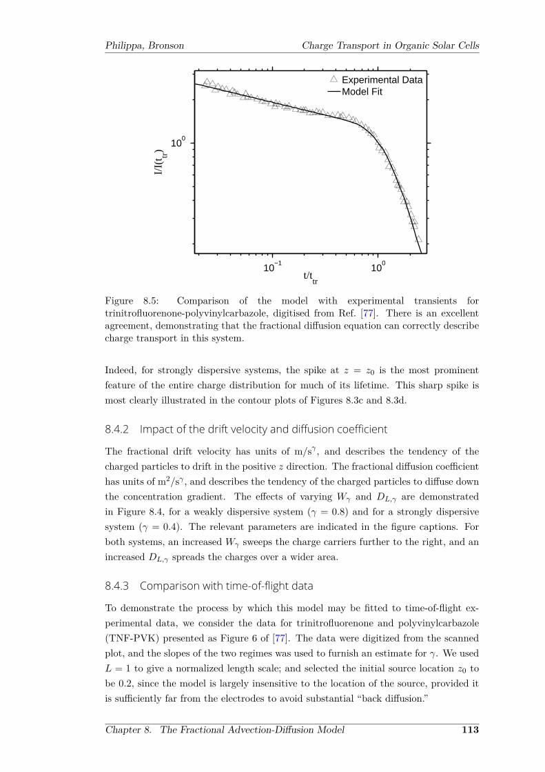
Philippa, Bronson Charge Transport in Organic Solar Cells
10−1
100
100
t/ttr
I/I(
t tr)
Experimental DataModel Fit
Figure 8.5: Comparison of the model with experimental transients fortrinitrofluorenone-polyvinylcarbazole, digitised from Ref. [77]. There is an excellentagreement, demonstrating that the fractional diffusion equation can correctly describecharge transport in this system.
Indeed, for strongly dispersive systems, the spike at z = z0 is the most prominentfeature of the entire charge distribution for much of its lifetime. This sharp spike ismost clearly illustrated in the contour plots of Figures 8.3c and 8.3d.
8.4.2 Impact of the drift velocity and diffusion coefficient
The fractional drift velocity has units of m/sγ , and describes the tendency of thecharged particles to drift in the positive z direction. The fractional diffusion coefficienthas units of m2/sγ , and describes the tendency of the charged particles to diffuse downthe concentration gradient. The effects of varying Wγ and DL,γ are demonstratedin Figure 8.4, for a weakly dispersive system (γ = 0.8) and for a strongly dispersivesystem (γ = 0.4). The relevant parameters are indicated in the figure captions. Forboth systems, an increased Wγ sweeps the charge carriers further to the right, and anincreased DL,γ spreads the charges over a wider area.
8.4.3 Comparison with time-of-flight data
To demonstrate the process by which this model may be fitted to time-of-flight ex-perimental data, we consider the data for trinitrofluorenone and polyvinylcarbazole(TNF-PVK) presented as Figure 6 of [77]. The data were digitized from the scannedplot, and the slopes of the two regimes was used to furnish an estimate for γ. We usedL = 1 to give a normalized length scale; and selected the initial source location z0 tobe 0.2, since the model is largely insensitive to the location of the source, provided itis sufficiently far from the electrodes to avoid substantial “back diffusion.”
Chapter 8. The Fractional Advection-Diffusion Model 113

Philippa, Bronson Charge Transport in Organic Solar Cells
The intercept of the two straight lines was taken to be the transit time ttr, and thefollowing equation was used to furnish an estimate of Wγ , which provided a startingpoint for curve fitting:
ttr ∼1
2
(L− z0Wγ
) 1γ
, (8.27)
the factor of 1/2 being an empirical correction that gives better results when comparedwith the order of magnitude estimate Eq. (8.26). There need not be a generalisedEinstein relation linking Wγ and DL,γ for such systems. However, to give an initialstarting point for the curve fitter, the diffusion coefficient was taken as DL,γ ≈Wγ/20.We note that the measured current is insensitive to diffusion because of the stronglydispersive transport that is present, and so the precise value of DL,γ is insignificant.
The parameter estimates discussed above were used as the starting point for non-linear least squares curve fitting. The Matlab Curve Fitting Toolbox was used. Theresult of the model fitting is shown in Figure 8.5. The fitted γ parameter is 0.83.
8.5 ConclusionWe have demonstrated a fractional advection diffusion equation modelling the hop-ping transport observed in many disordered semiconductors. We have shown that theinfinite series of Fourier modes [Eq. (8.5)] for the bounded solution can be collapsedinto a closed form expression using the Poisson summation theorem [Eq. (8.13)]. Itthis closed form expression that then facilitates the extraction of model parametersfrom the experimental data using a simple curve fitting routine. We have modelled atime of flight experiment by assuming the initial condition n(z, t0) = n0δ(z − z0). Wehave calculated the resultant electric current, and shown that the sum of slopes onlogarithmic axes is −2, as predicted by other models and as verified by experiment.It is possible to extend this solution to sources of finite duration or finite width, byintegrating with respect to t0 or z0, respectively.
Chapter 8. The Fractional Advection-Diffusion Model 114
9Generalised Diffusion Equations and
Fractional Kinetics
This chapter contains material that has been published in the following journal article:[4] Bronson Philippa, R. E. Robson, and R. D. White. Generalized phase-space
kinetic and diffusion equations for classical and dispersive transport. New Journal ofPhysics, 16, 073040 (2014). doi:10.1088/1367-2630/16/7/073040.
Ron White and Rob Robson supervised the work, derived the phase-space modeland its reduction to configuration space. It is simply stated here as the starting pointof this chapter. The interested reader is referred to the above publication for furtherdetails. The configuration space analysis, which formed the second half of the abovearticle, was performed by me and is presented here in greater detail than the abovepublication.
9.1 IntroductionThe previous chapters applied advection-diffusion equations to various transport prob-lems. The solution of these equations is a number density n(r, t). They are known as“configuration space” models, and are approximations of a more fundamental “phasespace” description that also includes velocity space. Configuration space approxima-tions are only valid in the hydrodynamic regime of smooth spatial gradients [207]. Itis therefore fortunate that many physical systems, including ordered semiconductors,rapidly approach this regime. Consequently, configuration space models are often anexcellent description of the dynamics of such materials.
115

Philippa, Bronson Charge Transport in Organic Solar Cells
A rapid approach to the hydrodynamic regime occurs when collisions dominate andmemory of the initial condition is lost after only a few collisions. Any large gradientsin the number density will be quickly smoothed. For such “classical” transport, thecorresponding diffusion equation is a conventional partial differential equation of firstorder in t and second order in r. Such systems are characterised by a diffusive regimewherein the mean square displacement grows linearly, i.e. ⟨x2⟩− ⟨x⟩2 ∼ t. In contrast,disordered semiconductors, such as those studied in this thesis, often demonstrate“anomalous” diffusion, wherein the mean square displacement is nonlinear, i.e. ⟨x2⟩ −⟨x⟩2 ∼ tγ where γ = 1 [77, 195,268,275].
Subdiffusion occurs when γ < 1. It arises from repeated trapping and de-trappingof the transported species, in which periods of “classical” transport are interrupted by(potentially long) periods of immobilisation. Consequently, the memory of the initialcondition may persist for long times, and large gradients are not necessarily smoothedout. As in the previous chapter, such effects are often accounted for by replacing theconventional time derivative with a fractional derivative [266,276–279]. The fractionalderivative accounts for the memory effects. However, the spatial gradient terms areleft intact, and thus the weak gradient assumption is therefore still implicit. This is anapparent contradiction that challenges the validity of the fractional diffusion equations.Until now, this issue has only been addressed in an ad-hoc manner, through solution ofan exactly solvable model kinetic equation in phase space [280]. The phase space systemdoes not require the assumption of weak gradients, so this questionable assumption isavoided. In that study [280], trapping effects were incorporated in the collision term,and even though the theory is consistent, it is nevertheless ad-hoc and warrants furtherscrutiny.
Recently, we resolved the ad-hoc nature of the previous approach by developingfrom first principles a new, physically-based, exactly solvable model kinetic equation[4]. A schematic of the fundamental processes is shown in Figure 9.1. Freely movingcarriers may be captured by trap states, where they are held for some period of timedrawn from a waiting time distribution ϕ(t). This distribution is defined such that theprobability of being released after an time in the interval t to t+ dt is ϕ(t)dt.
The resultant phase space model is [4]
(∂t + v · ∇+ a · ∂v) f = −ν [f − ϕ ∗ fdetrap] , (9.1)
where f is the free particle distribution function, a is the external acceleration, ν is arate constant for the trapping process, and fdetrap is the distribution function for thenewly detrapped carriers. We assume that the velocity distribution of these carriersis a Maxwellian. This is an arguable assumption, in that it assumes that de-trappedcarriers are effectively instantly thermalised with the medium temperature T . Theresulting distribution function is
fdetrap(r,v, t) = n(r, t)(
m
2πkBT
)3/2
exp(−m|v|22kBT
),
Chapter 9. Generalised Diffusion Equations and Fractional Kinetics 116

Philippa, Bronson Charge Transport in Organic Solar Cells
Velocity
Free carriers
Free states
Localised states
Trapping
De-trapping to a
Maxwellian distribution
of velocities
Free carriers
Trapped carriers
dx
dv
Position
Figure 9.1: Key processes occurring in the kinetic model. Freely moving chargesmay be scattered into localised states. The newly detrapped charges emerge with aMaxwellian distribution of velocities at the medium temperature.
where n(r, t) ≡´f(r,v, t)d3v is the number density, m is the carrier mass (or effective
mass), kB is the Boltzmann constant, and T is the medium temperature. Solving thismodel [4] for ideal time-of-flight conditions yields the “generalised diffusion equation”for the free charged particle density
∂n
∂t+ ν [1− ϕ∗]n+ vd
∂n
∂z−DL
∂2n
∂z2= 0, (9.2)
where vd is the drift velocity, and DL is the longitudinal diffusion coefficient. Notethat in contrast with the previous chapter, vd and DL are standard drift and diffusioncoefficients and do not have fractional units.
In this chapter, we shall analyse the generalised diffusion equation (9.2). We findthe analytic solution and then cast it into closed form by following the mathematicalprocedure that was developed in the previous chapter. Next, we analyse the role ofthe waiting time distribution ϕ, which is the key feature that differentiates Eq. (9.2)from other drift-diffusion models, including the fractional form from Chapter 8.
Chapter 9. Generalised Diffusion Equations and Fractional Kinetics 117

Philippa, Bronson Charge Transport in Organic Solar Cells
9.2 Formulation for Time-of-FlightAs in the previous chapter, we consider an ideal one-dimensional time-of-flight system.We introduce a slab of material of thickness L between two plane-parallel electrodes,the normal direction defining the z axis of the system of coordinates. We take absorbingboundary conditions, n(0, t) = n(L, t) = 0, and an impulse initial condition, n(z, 0) =n0δ(z − z0).
9.2.1 Series solution
Equation (9.2) is solved by separation of variables. We write n(z, t) = Z(z)T (t), andsubstitute into Eq. (9.2) to obtain:
T + ν[1− ϕ∗]TT
=−νdZ ′ +DLZ
′′
Z= c, (9.3)
where dots indicate time derivatives and primes indicate spatial derivatives, and c isan arbitrary separation constant. The spatial equation, i.e. the one involving Z, isidentical to the ordinary diffusion equation (without any trapping effects). Its solutionis
Z(z) =
∞∑m=1
Ameλz sin
(mπzL
), (9.4)
where λ ≡ vd/2DL and Am is an arbitrary constant of integration. The separationconstant c is negative and multi-valued:
cm = −m2π2DL
L2−DLλ
2. (9.5)
The temporal equation, which is unique to this model, is
T + ν[1− ϕ∗]T − cmT = 0.
The convolution hints that a Laplace transform might be useful. Solving this equationin Laplace space yields
T (s) =T (0)
s+ ν[1− ϕ(s)]− cm. (9.6)
Combining these according to the separation ansatz n = Z(z)T (t), the general solutionis
n(z, s) =
∞∑m=1
Ameλz sin
(mπzL
) 1
s+ ν[1− ϕ(s)]− cm, (9.7)
where T (0) has been merged into Am.
Chapter 9. Generalised Diffusion Equations and Fractional Kinetics 118

Philippa, Bronson Charge Transport in Organic Solar Cells
The integration constants Am will be specified by the initial condition. Using theinitial value theorem,
n(z, 0) = n0δ(z−z0) =∞∑
m=1
Ameλz sin
(mπzL
)lims→∞
1
1 + ν[1− ϕ(s)]s−1 − cms−1. (9.8)
The limit must converge to unity for any probability distribution1.This is a Fourier series, from which we find the Fourier coefficients Am to be
Am =2n0Le−λz0 sin
(mπz0L
). (9.9)
Combining all the above, the solution is
n(z, s) =
∞∑m=0
n0LDL
eλ(z−z0)cos[mπL−1 (z − z0)
]− cos
[mπL−1 (z + z0)
](s+ ν[1− ϕ(s)])D−1
L + λ2 +m2π2L−2. (9.10)
The transformation from sin to cos was done to facilitate the use of the Poisson sum-mation theorem.
9.2.2 Poisson Summation
As per the previous chapter, the Poisson summation theorem is useful in collapsinginfinite series like Eq. (9.10) into closed form. Recall that the Poisson summationtheorem is
∞∑m=−∞
f(mT ) =1
T
∞∑m=−∞
F(mT
), (9.11)
where F (k) is the Fourier transform of f(mT ). The first task is to write Eq. (9.10) inthe form of the left hand side of Eq. (9.11). We introduce the parameters
α =n0LDL
eλ(z−z0)
β2 = (s+ ν[1− ϕ(s)]) /DL + λ2
T =π
L
to obtainn(z, s) = α
∞∑m=0
cos [mT (z − z0)]− cos [mT (z + z0)]
β2 + (mT )2.
1The non-trivial term in the denominator is
lims→∞
ϕ(s)
s.
The numerator tends to zero in the limit of large s because the integrand vanishes exponentially
lims→∞
ϕ(s) = lims→∞
ˆ ∞
0
e−stϕ(t)dt → 0,
and consequently,lims→∞
ϕ(s)
s= 0.
All other terms on the denominator in (9.8) have trivial limits as s → ∞.
Chapter 9. Generalised Diffusion Equations and Fractional Kinetics 119

Philippa, Bronson Charge Transport in Organic Solar Cells
The limits of summation can be extended to −∞ because each term is an even functionof m:
n(z, s) =α
2
∞∑m=−∞
cos [mT (z − z0)]− cos [mT (z + z0)]
β2 + (mT )2.
Further, the cosine function can be replaced by the exponential representation
n(z, s) =α
2
∞∑m=−∞
eimT (z−z0) − eimT (z+z0)
β2 + (mT )2,
which is a valid transformation because the imaginary component of each exponentialis an odd function of m, and so all the imaginary components will cancel when thesummation is taken. This equation now resembles the left hand side of Eq. (9.11).
The next task is to take the Fourier transformation. The necessary integral is
F (k) =
ˆ ∞
−∞e−2πikτ e
iτ(z−z0) − eiτ(z+z0)
β2 + τ2dτ.
This integral can be evaluated using complex contours and the residue theorem. Theresult is
F (k) =π
β
[e−β|2πk−(z−z0)| − e−β|2πk−(z+z0)|
].
Finally, the Poisson summation theorem can be applied. We find
n(z, s) =α
2T
∞∑m=−∞
F(mT
)=
n02DLβ
eλ(z−z0)∞∑
m=−∞[exp (−β |2mL− (z − z0)|)− exp (−β |2mL− (z + z0)|)] .
By separately considering the cases of m < 0, m = 0, and m > 0, with the cases ofz < z0 and z > z0, this can be recognised as a geometric series with the closed formexpression
n(z, s) =n0e
λ(z−z0)
2DLβ
e−β|z−z0| − e−β|z+z0| − 4 sinh (βz) sinh (βz0)
e2βL − 1
. (9.12)
Equation (9.12) is the analytic solution to the time-of-flight problem.
9.2.3 Time-of-flight current
Since n(z, s) represents free charge, rather than total charge as in the last chapter, thecurrent expression is simply
j =vdL
ˆ L
0ndz
=vdn0
2LDLβ
ˆ L
0eλ(z−z0)
e−β|z−z0| − e−β|z+z0| − 4 sinh (βz) sinh (βz0)
e2βL − 1
dz.
Chapter 9. Generalised Diffusion Equations and Fractional Kinetics 120

Philippa, Bronson Charge Transport in Organic Solar Cells
10−4
10−3
10−2
10−1
100
101
102
10−3
10−2
10−1
100
Time, t / ttr
Cu
rre
nt,
j /
j 0
φ(t) = δ(t)
φ(t) = e−t/0.01
/0.01
φ(t) = e−t/0.03
/0.03
φ(s) = 1 − 0.1s
φ(s) = 1 − 0.3s
Figure 9.2: Modelled current transients for ideal time of flight experiments, showing theimpact of various waiting time distributions ϕ. Results are plotted in normalised units,where j0 is the initial current for the trap-free model, and ttr = L/vd is the trap-freetransit time. When ϕ(t) = δ(t) (top line), no trapping occurs. In the other cases, thetransients are influenced by trapping but the results exhibit “classical” transport withwell-defined drift velocities and diffusion coefficients. The trapping rate is ν = 103/ttr,the reciprocal of which gives the timescale for the transition to trap-limited transportin the case of an exponential waiting time distribution. The first moments of thewaiting time distribution functions from top to bottom are respectively 0, 0.01, 0.03,0.1, 0.3, in units of ttr. The dimensionless diffusion coefficient is DLttr/L
2 = 0.02.The initial delta-function pulse is at x0/L = 0.1. [In the legend, ϕ(s) is the Laplacetransform of ϕ(t).]
Evaluating this integral and simplifying,
j(s) =vdN(0)
(s+ ν [1− ϕ(s)])L
(1− e−λz0
[e−βz0 +
sinh (βz0)
sinh (βL)
(eλL − e−βL
)]). (9.13)
To this point the discussion is quite general, but to go further, we must specifyϕ(t).
9.3 Role of the waiting time distribution
9.3.1 Waiting time distributions ϕ(t) with a finite first moment---'classical'transport
To study the impact of the waiting time distribution on the solution, we initiallyconsidered several simple ϕ(t) functions. Time of flight transients were calculatedusing Eq. (9.13), numerically inverting the Laplace transform. Dimensionless resultsare shown in Figure 9.2, where time is scaled to the transit time ttr = L/vd through a
Chapter 9. Generalised Diffusion Equations and Fractional Kinetics 121

Philippa, Bronson Charge Transport in Organic Solar Cells
sample of thickness L, and concentration is scaled to the initial concentration N(0). Inthis system of units, the normalised drift velocity is equal to 1. We set the normaliseddiffusion coefficient to DLttr/L
2 = 0.02.The simplest choice for the waiting time distribution is the Dirac delta, ϕ(t) = δ(t).
In this case, de-trapping occurs instantaneously and consequently has no impact. Thesystem reduces to the standard advection-diffusion equation.
Another choice is an exponential distribution, ϕ(t) = e−t/τ/τ . Two examples withexponential distributions are shown in Figure 9.2, which different first moments, τ .The initial trap-free transport transitions into trap-limited transport on a timescalegoverned by the collision frequency (∼ ν−1). The trap-limited transport is charac-terised by an increased transit time (and hence decreased effective drift velocity) forincreased τ because of the additional time spent in traps. For the same reason, thecurrent density j falls with increased τ . Nevertheless, the transport is not dispersive,and there exists a clear time-of-flight arrival time.
A final option explored is a first-order truncation of the series expansion of theexponential waiting time distribution in Laplace space: ϕ(s) ∼ 1−τs, where again τ isthe first moment of the waiting time distribution function. As can be seen from Figure9.2, the first moment of ϕ controls the long-time behaviour. Higher moments can onlyinfluence the behaviour at shorter times, as is demonstrated by the differences betweenthe cases with an exponential distribution and those with the Laplace domain seriesexpansion.
9.3.2 Relating the waiting time distribution to a density of trapped states
Rather than simply assuming an ad-hoc waiting time distribution, it may be usefulto calculate it from a more fundamental physical model. In what follows, we give aspecific example for how this might be achieved. We consider a semiconductor withtraps that form a density of localized states below the band gap. The release timesϕ(t) are determined by the distribution of these traps in energy space.
To describe this semiconductor, we use a multiple trapping model with a uniformcapture (trapping) cross-section [212] for charge carriers. We define the density oflocalised states to be g(ϵ), where ϵ < 0 is the energy relative to the conduction band.If the rate of escape from a trap at energy ϵ is proportional to exp(ϵ/kBT ) then
ϕ(t) = ν0
ˆ 0
−∞g(ϵ)eϵ/kBT exp
−tν0eϵ/kBT
dϵ, (9.14)
where ν0 is a frequency characterizing the rate of escape from traps. The densityof states g(ϵ) can be measured experimentally [222, 281]. In this case we assumean exponential distribution, which occurs in certain organic and inorganic materials[12, 120]. Then g(ϵ) = eϵ/kBTc/kTc, where Tc is a characteristic temperature thatdescribes the width of the density of states. Eq. (9.14) yields
ϕ(t) = αν0 (tν0)−α−1 γ (α+ 1, tν0) , (9.15)
Chapter 9. Generalised Diffusion Equations and Fractional Kinetics 122

Philippa, Bronson Charge Transport in Organic Solar Cells
10−6
10−5
10−4
10−3
10−2
10−1
100
α = T/Tc = 0.5
Cu
rre
nt,
j /
j0
νttr = 10
4
νttr = 10
3
νttr = 10
2
νttr = 10
νttr = 0
10−6
10−5
10−4
10−3
10−2
10−1
100
101
102
103
104
105
10−6
10−5
10−4
10−3
10−2
10−1
100
νttr = 10
4
Time, t / ttr
Cu
rre
nt,
j /
j0
α = T/Tc = 0.5
α = T/Tc = 0.6
α = T/Tc = 0.7
α = T/Tc = 0.8
α = T/Tc = 0.9
Figure 9.3: Modelled current transients for ideal time of flight experiments using thewaiting time distribution (9.15), which was calculated for a semiconductor with anexponential distribution of localised states. An initial trap-free regime transitions intostrongly-trap limited dispersive transport. Transport parameters are the same as Fig.2, except for the alternative waiting time distribution. These plots were calculated forν0ttr = 5 × 10⁵. The transition between “classical” and dispersive regimes occurs att/ttr ∼ (νttr)
−1.
Chapter 9. Generalised Diffusion Equations and Fractional Kinetics 123

Philippa, Bronson Charge Transport in Organic Solar Cells
where γ(·, ·) is the lower incomplete Gamma function2, and α = T/Tc. This distri-bution appears in the literature of the multiple trapping model, for example, Eqn (9)of Ref. [213]. This distribution is normalized, and it has a divergent first moment,sufficient to describe dispersive transport [192,282,283].
Figure 9.3 shows typical time of flight transients together the waiting time distri-bution Eq. (9.15). Initially, all carriers are assumed to be untrapped. At short timesthe profiles are classical, with a transition to dispersive behaviour at longer times asthe carriers begin to enter the trap states. In the dispersive regime, the sum of slopesis -2, exactly as expected for an exponential density of states [77]. We note that adifferent form of dispersive transport may arise from a different density of states, andthat our model can be readily adapted by evaluating Eq. (9.14) with the appropriateg(ϵ) function.
The parameters used for Figure 9.3 were chosen as follows. The attempt to escapefrequency ν0 is extremely fast (e.g. ∼ 1012 Hz for a realistic system [212]), so weconsider only the situation where ν0ttr ≫ 1. We selected ν0ttr = 5 × 10⁵ for Figure9.3. The trapping frequency ν, which is a new feature of our model, must be largeenough that νttr > 1, otherwise there will be negligible trapping events before the timeof flight experiment has concluded. In Figure 9.3 (a), we demonstrate the influenceof this parameter. It controls the time scale for the transition between classical anddispersive transport. Finally, if the transport is dispersive, the temperature T mustbe below the critical temperature Tc [212]. We examine the range 0.5 ≤ T/Tc ≤ 0.9 inFigure 9.3 (b). It can be seen that the slope of the current transient is controlled bythe temperature.
Our generalised diffusion equation (9.2) provides a framework for a unified analysisof transport, whether dispersive or classical. It is pertinent at this point to highlightthat in the long time limit, one can make direct connection to the fractional diffusionequation literature [192,282,283]. If we consider the Laplace transform of the waitingtime distribution Eq. (9.15)
ϕ(s) = − απ
sinαπ
(s
ν0
)α
+ 2F1
(1,−α; 1− α;− s
ν0
), (9.16)
where 2F1 is a hypergeometric function, then the small s (long time) representation ofthis is
ϕ(s) ≈ 1− rαsα. (9.17)
Here the coefficients of the sα term have been collected into a single parameter rα ≡ν−α0 απ/ sinαπ, which weights the relative importance of trapping effects. By substi-
tuting Eq. (9.17) into (9.2), and taking the limit of small s, one obtains a fractionaldiffusion equation, with a Riemann-Liouville or Caputo form of the fractional deriv-ative depending upon whether one solves for untrapped charge or total charge. Thesefractional equations result from a waiting time distribution that was calculated using
2The lower incomplete gamma function is γ(a, z) ≡´ z
0ta−1e−tdt.
Chapter 9. Generalised Diffusion Equations and Fractional Kinetics 124

Philippa, Bronson Charge Transport in Organic Solar Cells
an exponential density of trap states. It remains to be seen whether alternative “frac-tional” equations could be formed by considering different distributions for the densityof trapped states.
9.4 Concluding remarksIn this chapter we have studied a generalized diffusion equation (9.2) for transport indisordered materials. This equation is grounded in a phase-space kinetic model thataccounts for both free particle transport and trapping/detrapping from localized states,described by a waiting time function ϕ(t). This model provides a unified frameworkfor the analysis of transport, whether dispersive or not. The nature of the transportis strongly influenced by the waiting time distribution, and in particular, the firstmoment of this distribution plays a dominant role. By way of example, this model wasapplied to a disordered semiconductor, obtaining dispersive transport if the density ofstates is exponential. Other distributions (e.g. a Gaussian) might be expected to yielddifferent detailed behaviour, which could be calculated using the generalized diffusionequation presented here.
Chapter 9. Generalised Diffusion Equations and Fractional Kinetics 125
10Conclusion
10.1 SummaryCharge transport is a key contributor to the performance of any electronic device.In the specific case of organic solar cells, high power conversion efficiencies can onlybe achieved if charges are quickly extracted without significant recombination losses.The charge transport properties of current organic photovoltaics are inadequate, forexample if device thicknesses are to be increased for optimal light harvesting, or be-cause of inhomogeneities in large-scale fabrication. There is a need for better tools toquantify charge transport, which should lead to improved physical understanding andperhaps guide future performance gains. This thesis addressed these issues with thedevelopment of new experimental techniques that contributed physical insights intothe charge transport mechanisms in a variety of OPV systems.
There is a huge design space of charge transport experiments that can be conceivedusing only a light source, arbitrary waveform generator, variable load resistor, andoscilloscope. Over the course of this project, many such experimental configurationswere simulated. The simulations quickly identified those which were most promisingin terms of robustness and accuracy, and also excluded many that were intuitivelyplausible but did not stand up to the rigorous analysis provided by the simulationsoftware. The most promising techniques were further refined, using the simulationsto learn how to recognise and work with non-ideal effects such as charge trappingand dispersive transport. Armed with the knowledge gained from the simulations, thisthesis addressed questions of scientific importance regarding the impact of hot carriers,charge carrier thermalisation, and recombination.
126

Philippa, Bronson Charge Transport in Organic Solar Cells
Charge carrier thermalisation, in the form of a time-dependent mobility, wasstudied in three different polymer:fullerene blends using two different experimentaltechniques. The photo-CELIV technique was applied to poly[3,6-dithiophene-2-yl-2,5-di(2-octyldodecyl)-pyrrolo[3,4-c]pyrrole-1,4-dione-alt-naphthalene] (PDPP-TNT) :[6,6] phenyl-C71-butyric-acid-methyl-ester (PC70BM) [220] solar cells. A shift in thecurrent maximum with increasing delay time was observed, as has previously beenreported in other organic solar cell systems [137, 138]. However, numeric simulationwith a drift-diffusion model demonstrated that this shift is induced by the measure-ment technique and does not necessarily indicate a genuine time-dependence in themobility. Quantitative analysis of the observed data revealed that carrier mobility isnot time-dependent in this system. This highlights a weakness of the photo-CELIVtechnique: variations in the experimental conditions might induce artificial trends intothe apparent mobility. We also examined the impact of dispersion on photo-CELIVtransients, and found that a systematic change in the apparent mobility occurs whenthe amount of dispersion is varied, even if the true mobility is held constant. Thiswould be complicate temperature-dependent studies, since the amount of dispersion isoften dependent upon temperature. It was concluded that care must be taken whenexamining trends in mobility obtained via photo-CELIV.
Next, carrier relaxation was studied in poly[N-9”-hepta-decanyl-2,7-carbazole-alt-5,5-(4’,7’-di-2-thienyl-2’,1’,3’-benzothiadiazole)] (PCDTBT):PC70BM and poly[[4,8-bis-[(2-ethylhexyl)oxy]benzo[1,2-b:4,5-b’]dithiophene-2,6-diyl][3-fluoro-2-[(2-ethylhexyl)car-bonyl]thieno[3,4-b]thiophenediyl]] (PTB7):PC70BM. These experiments were performedusing the novel technique of Resistance dependent PhotoVoltage (RPV), which was de-veloped in order to address the limitations of photo-CELIV. There was no evidenceof any time-dependent mobility as the transit time was varied by changing the biasvoltage and device thickness. Similarly, there was no evidence of energetic relaxa-tion extending to the timescale of charge transport when different wavelengths of laserpumping were used. This is in contrast to the prediction of the influential Gaus-sian Disorder Model that dispersive transport arises due to the energetic relaxationof charge carriers. Our observations are inconsistent with this hypothesis, and so weargue that dispersion in these systems is instead caused by charge trapping, and thereduction in photocurrent that is typically attributed to a time-dependent mobility isactually driven by the gradual loss of charges to deep trap states.
To study recombination, the RPV technique was extended to high light intensities(HI-RPV). It was shown that low molecular weight PCDTBT (Mn = 4.3 kDa, Mw
= 12.1 kDa, PDI = 2.8) results in Langevin recombination, whereas high molecularweight PCDTBT (Mn = 22.7 kDa, Mw = 122.2 kDa, PDI = 5.4) results in non-Langevin recombination with a reduction factor β/βL ≈ 0.07. This highlights thatmolecular weight may need to be considered when optimising devices.
Next, we studied the steady-state short-circuit current as a function of light intens-ity, which we call IPC, or intensity-dependent photocurrent. Simulations identifiedthat there is a critical threshold at which charge transport becomes inadequate and
Chapter 10. Conclusion 127

Philippa, Bronson Charge Transport in Organic Solar Cells
substantial non-geminate recombination begins. This threshold is the space-chargelimited current, Isclc ∼
√βL/β CU/tslower
tr , from which the required mobility, recom-bination coefficient, device thickness, dielectric permittivity, and voltage can be calcu-lated. We experimentally verified this prediction using solar cells of varying thicknessmade from PCDTBT:PC70BM and PTB7:PC70BM.
The second theme of this thesis was related to generalised (or “fractional”) trans-port models. It was demonstrated that the Poisson summation theorem is applicableto the analytic solution of a fractional advection-diffusion equation. With the use ofthe Poisson summation theorem, the result can be expressed concisely in closed formin Laplace space. This is helpful in manipulating the analytic solution of such models.Finally, a new form of generalised kinetic model was proposed and analysed. This kin-etic model introduces trapping and de-trapping into phase space, with the de-trappingmechanism specified via a waiting time probability density function. It was shown thatdiffering choices of the waiting time distribution result in qualitatively different typesof charge transport, and in particular, that the proposed kinetic model incorporatesboth normal and dispersive transport within the same common framework.
10.2 Recommendations for Future WorkThis is a broad field and there are many opportunities, but we have identified severalissues that directly arise from this work and can be addressed using the frameworkand tools that we have developed.
Analysis of recombination via photo-CELIV—In Chapter 4, we demonstrated thatphoto-CELIV measurements of the time-, field-, and temperature-dependence of mo-bility may be misleading due to variations in the shape of the photo-CELIV transient.The photo-CELIV technique is also used to study recombination, and it seems likelythat similar artefacts would affect recombination studies too. It is recommended thatsimulations and experiments be performed in order to understand the impact of thedelay time, charge trapping, and dispersive transport on recombination measurements.
Time-dependent mobility in pristine polymers—We have shown in Chapters 4 and5 that three polymer:fullerene systems display no evidence of mobility relaxation onthe timescales of charge transport, despite the fact that such dependencies have pre-viously been reported (often with the photo-CELIV technique). An interesting testcase that we have not yet explored is whether there is any energetic relaxation in purepolymer films, as opposed to polymer:fullerene blends. This would provide insight intothe microscopic transport mechanism that applies in polymer domains and/or at theinterface between polymers and fullerenes.
Impact of trapping on HI-RPV—The HI-RPV technique (Chapter 6) encountersdifficulties in the presence of deep trapping. The extracted charge does not saturateto CU in the limit of large resistances, but instead to a value approximately 2-5 timeshigher than CU . We performed some preliminary simulations that demonstrated thiseffect when a substantial quantity of charge is trapped for long periods of time, but
Chapter 10. Conclusion 128

Philippa, Bronson Charge Transport in Organic Solar Cells
due to the time constraints of this thesis, this work was not yet completed. Furtheranalysis is needed in order to develop useful predictive tools.
Applying the Poisson summation theorem to other fractional equations—The Pois-son summation theorem was shown to be useful in the analytic solution of a time-fractional Caputo diffusion equation (Chapter 8), and a generalised diffusion equationwith a convolution term (Chapter 9). Given it was useful in these two distinct systems,it is likely that other types of fractional equation would benefit from a similar treat-ment. Many different fractional equations have been applied in the literature, and soit is likely that some of these would be amenable to the techniques presented here.
Dispersive transport with non-exponential density-of-states distributions—The gen-eralised diffusion model in Chapter 9 produces standard Scher-Montroll dispersivetransport when an exponential density-of-states (DOS) is used. However, some or-ganic materials display different distributions, for example a Gaussian. To adapt themodel for a different DOS, one evaluates the release time integral [Eq. (9.14)] for thenew distribution. It would be interesting to examine whether other types of distribu-tion can give rise to different types of dispersive transport, for example, whether the“sum of slopes” can be varied from the Scher-Montroll/exponential DOS value of −2.
Dispersive to non-dispersive transitions—Fractional models for subdiffusion exhibitinstability in the presence of spatially varying fractional order [284, 285], as might beexpected to arise in practice due to inhomogeneities in the material if the fractionalorder depends upon the material structure or properties. This is an important issue be-cause spatial variations might be especially likely in disordered media, precisely wherethe existing (unstable) models are intended to be used! Preliminary analysis indicatesthat the model described in Chapter 9 can avoid this problem by an appropriate choiceof waiting time distribution that triggers a transition to non-dispersive transport atlong times. It is recommended that the transition to non-dispersion be investigated asa mechanism to prevent the structural instability in the fractional models.
Higher moments of the kinetic equation—In Chapter 9, the generalised kineticmodel was integrated over all velocities to obtain a particle balance. Higher ordermoments in velocity space can be used to obtain, for example, a momentum balanceand an energy balance. These are likely to contain information about relaxation effectsthat are associated with charge trapping, and possibly fields that are rapidly varyingin time or space.
Chapter 10. Conclusion 129
References
[1] B. W. Philippa, R. D. White, and R. E. Robson. Analytic solutionof the fractional advection-diffusion equation for the time-of-flight exper-iment in a finite geometry. Physical Review E, 84, 041138 (2011).doi:10.1103/PhysRevE.84.041138.
[2] Bronson Philippa, Martin Stolterfoht, Ronald D. White, Marrapan Velusamy,Paul L. Burn, Paul Meredith, and Almantas Pivrikas. Molecular weight depend-ent bimolecular recombination in organic solar cells. The Journal of ChemicalPhysics, 141, 054903 (2014). doi:10.1063/1.4891369.
[3] Bronson Philippa, Martin Stolterfoht, Paul L Burn, Gytis Juška, Paul Meredith,Ronald D White, and Almantas Pivrikas. The impact of hot charge carriermobility on photocurrent losses in polymer-based solar cells. Scientific Reports,4, 5695 (2014). doi:10.1038/srep05695.
[4] Bronson Philippa, R. E. Robson, and R. D. White. Generalized phase-spacekinetic and diffusion equations for classical and dispersive transport. New Journalof Physics, 16, 073040 (2014). doi:10.1088/1367-2630/16/7/073040.
[5] Bronson Philippa, Chellappan Vijila, Ronald D. White, Prashant Sonar, Paul L.Burn, Paul Meredith, and Almantas Pivrikas. Time-independent charge carriermobility in a model polymer:fullerene organic solar cell. Organic Electronics, 16,205 (2015). doi:10.1016/j.orgel.2014.10.047.
[6] Ardalan Armin, Gytis Juška, Bronson W. Philippa, Paul L. Burn, Paul Meredith,Ronald D. White, and Almantas Pivrikas. Doping-induced screening of the built-in-field in organic solar cells: Effect on charge transport and recombination.Advanced Energy Materials, 3, 321 (2013). doi:10.1002/aenm.201200581.
[7] Chellappan Vijila, Samarendra P Singh, Evan Williams, Prashant Sonar, Al-mantas Pivrikas, Bronson Philippa, Ronald White, Elumalai Naveen Kumar,S. Gomathy Sandhya, Sergey Gorelik, Jonathan Hobley, Akihiro Furube, Hiroy-uki Matsuzaki, and Ryuzi Katoh. Relation between charge carrier mobility andlifetime in organic photovoltaics. Journal of Applied Physics, 114, 184503 (2013).doi:10.1063/1.4829456.
[8] Martin Stolterfoht, Bronson Philippa, Ardalan Armin, Ajay K. Pandey, Ron-ald D. White, Paul L. Burn, Paul Meredith, and Almantas Pivrikas. Advantage
130

Philippa, Bronson Charge Transport in Organic Solar Cells
of suppressed non-Langevin recombination in low mobility organic solar cells.Applied Physics Letters, 105, 013302 (2014). doi:10.1063/1.4887316.
[9] Peter W. Stokes, Bronson Philippa, Wayne Read, and Ronald D. White. Efficientnumerical solution of the time fractional diffusion equation by mapping fromits Brownian counterpart. Journal of Computational Physics, 282, 334 (2015).doi:10.1016/j.jcp.2014.11.023.
[10] George Malliaras and Richard Friend. An Organic Electronics Primer. PhysicsToday, 58, 53 (2005). doi:10.1063/1.1995748.
[11] Christoph J Brabec, Srinivas Gowrisanker, Jonathan J M Halls, Darin Laird,Shijun Jia, and Shawn P Williams. Polymer-fullerene bulk-heterojunction solarcells. Advanced Materials, 22, 3839 (2010). doi:10.1002/adma.200903697.
[12] Carsten Deibel and Vladimir Dyakonov. Polymer-fullerene bulk heterojunctionsolar cells. Reports on Progress in Physics, 73, 096401 (2010). doi:10.1088/0034-4885/73/9/096401.
[13] A. Mayer, S. Scully, B. Hardin, M. Rowell, and M. McGehee. Polymer-basedsolar cells. Materials Today, 10, 28 (2007). doi:10.1016/S1369-7021(07)70276-6.
[14] Harald Hoppe and Niyazi Serdar Sariciftci. Organic solar cells: An overview.Journal of Materials Research, 19, 1924 (2004). doi:10.1557/JMR.2004.0252.
[15] Stephen R. Forrest. The path to ubiquitous and low-cost organic electronicappliances on plastic. Nature, 428, 911 (2004).
[16] John A. Rogers, Takao Someya, and Yonggang Huang. Materialsand mechanics for stretchable electronics. Science, 327, 1603 (2010).doi:10.1126/science.1182383.
[17] Matthew S. White, Martin Kaltenbrunner, Eric D. Glowacki, Kateryna Gut-nichenko, Gerald Kettlgruber, Ingrid Graz, Safae Aazou, Christoph Ulbricht,Daniel A. M. Egbe, Matei C. Miron, Zoltan Major, Markus C. Scharber, Tsuy-oshi Sekitani, Takao Someya, Siegfried Bauer, and Niyazi Serdar Sariciftci. Ul-trathin, highly flexible and stretchable PLEDs. Nature Photonics, 7, 811 (2013).doi:10.1038/nphoton.2013.188.
[18] Frederik C. Krebs. Fabrication and processing of polymer solar cells: A reviewof printing and coating techniques. Solar Energy Materials and Solar Cells, 93,394 (2009). doi:10.1016/j.solmat.2008.10.004.
[19] Martin A Green, Keith Emery, Yoshihiro Hishikawa, Wilhelm Warta, andEwan D Dunlop. Solar cell efficiency tables (version 43). Progress in Photo-voltaics: Research and Applications, 22, 1 (2014). doi:10.1002/pip.2452.
References 131

Philippa, Bronson Charge Transport in Organic Solar Cells
[20] L. Koster, E. Smits, V. Mihailetchi, and P. Blom. Device model for the operationof polymer/fullerene bulk heterojunction solar cells. Physical Review B, 72,085205 (2005). doi:10.1103/PhysRevB.72.085205.
[21] M.T. Neukom, N.A. Reinke, and B. Ruhstaller. Charge extraction with linearlyincreasing voltage: A numerical model for parameter extraction. Solar Energy,85, 1250 (2011). doi:10.1016/j.solener.2011.02.028.
[22] M.T. Neukom, S. Züfle, and B. Ruhstaller. Reliable extraction of organic solarcell parameters by combining steady-state and transient techniques. OrganicElectronics, 13, 2910 (2012). doi:10.1016/j.orgel.2012.09.008.
[23] I M Sokolov and J Klafter. From diffusion to anomalous diffusion: a centuryafter Einstein’s Brownian motion. Chaos (Woodbury, N.Y.), 15, 26103 (2005).doi:10.1063/1.1860472.
[24] Eli Barkai. CTRW pathways to the fractional diffusion equation. ChemicalPhysics, 284, 13 (2002). doi:10.1016/S0301-0104(02)00533-5.
[25] Benoît Robyns, Arnaud Davigny, Bruno François, Antoine Henneton, andJonathan Sprooten. Electricity Production from Renewables Energies. Wiley(2012). ISBN 9781118563069.
[26] Wallace C.H. Choy (Editor). Organic Solar Cells. Green Energy and Technology.Springer, London (2013). ISBN 978-1-4471-4822-7. doi:10.1007/978-1-4471-4823-4.
[27] Stephen R Forrest. The Limits to Organic Photovoltaic Cell Efficiency. MRSBulletin, 30, 28 (2005). doi:10.1557/mrs2005.5.
[28] American Society for Testing and Materials. Reference Solar Spectral Irradiance:Air Mass 1.5.
[29] Ardalan Armin, Marappan Velusamy, Pascal Wolfer, Yuliang Zhang, Paul LBurn, Paul Meredith, and Almantas Pivrikas. Quantum Efficiency of OrganicSolar Cells: Electro-Optical Cavity Considerations. ACS Photonics, 1, 173(2014). doi:10.1021/ph400044k.
[30] Yasuhiko Shirota and Hiroshi Kageyama. Charge carrier transporting molecularmaterials and their applications in devices. Chemical reviews, 107, 953 (2007).doi:10.1021/cr050143+.
[31] Nieves Espinosa, Rafael García-Valverde, Antonio Urbina, and Frederik C.Krebs. A life cycle analysis of polymer solar cell modules prepared using roll-to-roll methods under ambient conditions. Solar Energy Materials and Solar Cells,95, 1293 (2010). doi:10.1016/j.solmat.2010.08.020.
References 132

Philippa, Bronson Charge Transport in Organic Solar Cells
[32] Martin Kaltenbrunner, Matthew S White, Eric D Glowacki, Tsuyoshi Sekitani,Takao Someya, Niyazi Serdar Sariciftci, and Siegfried Bauer. Ultrathin andlightweight organic solar cells with high flexibility. Nature Communications, 3,770 (2012). doi:10.1038/ncomms1772.
[33] Gilles Dennler, Niyazi Serdar Sariciftci, and Christoph J. Brabec. ConjugatedPolymer-Based Organic Solar Cells. In Semiconducting Polymers: Chemistry,Physics and Engineering, edited by Georges Hadziioannou and George G. Malli-aras, chapter 11, 455–530. WILEY-VCH Verlag GmbH & Co. KGaA, Weinheim,second edition (2007). ISBN 978-3-527-31271-9.
[34] Jenny Nelson. Polymer:fullerene bulk heterojunction solar cells. Materials Today,14, 462 (2011). doi:10.1016/S1369-7021(11)70210-3.
[35] Ian H Campbell, Brian K Crone, and Darryl L Smith. Physics of Organic Light-Emitting Diodes. In Semiconducting Polymers: Chemistry, Physics and Engin-eering, edited by Georges Hadziioannou and George G Malliaras, chapter 10,421–454. WILEY-VCH Verlag GmbH & Co. KGaA, Weinheim, second edition(2007). ISBN 978-3-527-31271-9.
[36] Nir Tessler. Lasers Based on Semiconducting Organic Materials. AdvancedMaterials, 11, 363 (1999). doi:10.1002/(SICI)1521-4095(199903)11:5<363::AID-ADMA363>3.0.CO;2-Y.
[37] I D W Samuel and G a Turnbull. Organic semiconductor lasers. Chemicalreviews, 107, 1272 (2007). doi:10.1021/cr050152i.
[38] Gilles Horowitz. Organic Field-Effect Transistors. Advanced Materi-als, 10, 365 (1998). doi:10.1002/(SICI)1521-4095(199803)10:5<365::AID-ADMA365>3.0.CO;2-U.
[39] Giles Horowitz. Organic Thin-Film Transistors. In Semiconducting Poly-mers: Chemistry, Physics and Engineering, edited by Georges Hadziioannouand George G Malliaras, chapter 12, 531–566. WILEY-VCH Verlag GmbH &Co. KGaA, Weinheim, second edition (2007). ISBN 978-3-527-31271-9.
[40] Henning Sirringhaus. 25th anniversary article: organic field-effect transistors:the path beyond amorphous silicon. Advanced Materials, 26, 1319 (2014).doi:10.1002/adma.201304346.
[41] Hee Taek Yi, Marcia M. Payne, John E. Anthony, and Vitaly Podzorov. Ultra-flexible solution-processed organic field-effect transistors. Nature Communica-tions, 3, 1259 (2012). doi:10.1038/ncomms2263.
[42] Yang Yang, Jianyong Ouyang, Liping Ma, Jia-Hung Tseng, and Chih-Wei Chu.Organic/Polymeric Thin-Film Memory Devices. In Semiconducting Polymers:Chemistry, Physics and Engineering, edited by Georges Hadziioannou and
References 133

Philippa, Bronson Charge Transport in Organic Solar Cells
George G Malliaras, chapter 15, 613–642. WILEY-VCH Verlag GmbH & Co.KGaA, Weinheim, second edition (2007). ISBN 978-3-527-31271-9.
[43] Hoang-Anh Ho and Mario Leclerc. Biosensors Based on Conjugated Polymers.In Semiconducting Polymers: Chemistry, Physics and Engineering, edited byGeorges Hadziioannou and George G Malliaras, chapter 16, 643–666. WILEY-VCH Verlag GmbH & Co. KGaA, Weinheim, second edition (2007). ISBN 978-3-527-31271-9.
[44] Holger Spanggaard and Frederik C. Krebs. A brief history of the developmentof organic and polymeric photovoltaics. Solar Energy Materials and Solar Cells,83, 125 (2004). doi:10.1016/j.solmat.2004.02.021.
[45] C. W. Tang. Two-layer organic photovoltaic cell. Applied Physics Letters, 48,183 (1986). doi:10.1063/1.96937.
[46] N. S. Sariciftci, L. Smilowitz, A. J. Heeger, and F. Wudl. Photoinduced electrontransfer from a conducting polymer to buckminsterfullerene. Science, 258, 1474(1992). doi:10.1126/science.258.5087.1474.
[47] S Matthew Menke, Wade a Luhman, and Russell J Holmes. Tailored excitondiffusion in organic photovoltaic cells for enhanced power conversion efficiency.Nature Materials, 12, 152 (2012). doi:10.1038/nmat3467.
[48] Paul E. Shaw, Arvydas Ruseckas, and Ifor D. W. Samuel. Exciton DiffusionMeasurements in Poly(3-hexylthiophene). Advanced Materials, 20, 3516 (2008).doi:10.1002/adma.200800982.
[49] Tracey M Clarke and James R Durrant. Charge photogeneration in organic solarcells. Chemical reviews, 110, 6736 (2010). doi:10.1021/cr900271s.
[50] G. Yu, J. Gao, J. C. Hummelen, F. Wudl, and A. J. Heeger. Polymer Photo-voltaic Cells: Enhanced Efficiencies via a Network of Internal Donor-AcceptorHeterojunctions. Science, 270, 1789 (1995). doi:10.1126/science.270.5243.1789.
[51] Jan C. Hummelen, Brian W Knight, F. LePeq, Fred Wudl, Jie Yao, andCharles L. Wilkins. Preparation and Characterization of Fulleroid and Meth-anofullerene Derivatives. The Journal of Organic Chemistry, 60, 532 (1995).doi:10.1021/jo00108a012.
[52] Mikkel Jø rgensen, Jon E. Carlé, Roar R. Sø ndergaard, Marie Lauritzen,Nikolaj A. Dagnæ s Hansen, Sedi L. Byskov, Thomas R. Andersen, Thue T.Larsen-Olsen, Arvid P.L. Böttiger, Birgitta Andreasen, Lei Fu, Lijian Zuo, YaoLiu, Eva Bundgaard, Xiaowei Zhan, Hongzheng Chen, and Frederik C. Krebs.The state of organic solar cells—A meta analysis. Solar Energy Materials andSolar Cells, 1–10 (2013). doi:10.1016/j.solmat.2013.05.034.
References 134

Philippa, Bronson Charge Transport in Organic Solar Cells
[53] L. Jan Anton Koster, Sean E. Shaheen, and Jan C. Hummelen. Pathways to aNew Efficiency Regime for Organic Solar Cells. Advanced Energy Materials, 2,1246 (2012). doi:10.1002/aenm.201200103.
[54] Brian A. Gregg. The Photoconversion Mechanism of Excitonic Solar Cells. MRSBulletin, 30, 20 (2005). doi:10.1557/mrs2005.3.
[55] V. I. Arkhipov, P. Heremans, and H. Bässler. Why is exciton dissociation soefficient at the interface between a conjugated polymer and an electron acceptor?Applied Physics Letters, 82, 4605 (2003). doi:10.1063/1.1586456.
[56] Peter Peumans and Stephen R. Forrest. Separation of geminate charge-pairs atdonor–acceptor interfaces in disordered solids. Chemical Physics Letters, 398,27 (2004). doi:10.1016/j.cplett.2004.09.030.
[57] Carsten Deibel, Thomas Strobel, and Vladimir Dyakonov. Origin of the EfficientPolaron-Pair Dissociation in Polymer-Fullerene Blends. Physical Review Letters,103, 036402 (2009). doi:10.1103/PhysRevLett.103.036402.
[58] G. Grancini, M. Maiuri, D. Fazzi, A. Petrozza, H-J. Egelhaaf, D. Brida,G. Cerullo, and G. Lanzani. Hot exciton dissociation in polymer solar cells.Nature Materials, 12, 29 (2013). doi:10.1038/nmat3502.
[59] Koen Vandewal, Steve Albrecht, Eric T. Hoke, Kenneth R. Graham, JohannesWidmer, Jessica D. Douglas, Marcel Schubert, William R. Mateker, Jason T.Bloking, George F. Burkhard, Alan Sellinger, Jean M. J. Fréchet, Aram Amas-sian, Moritz K. Riede, Michael D. McGehee, Dieter Neher, and Alberto Salleo.Efficient charge generation by relaxed charge-transfer states at organic interfaces.Nature materials, 13, 63 (2014). doi:10.1038/nmat3807.
[60] Simon Gélinas, Akshay Rao, Abhishek Kumar, Samuel L Smith, Alex W Chin,Jenny Clark, Tom S van der Poll, Guillermo C Bazan, and Richard H Friend.Ultrafast Long-Range Charge Separation in Organic Semiconductor PhotovoltaicDiodes. Science, 512 (2013). doi:10.1126/science.1246249.
[61] Arun Aby Paraecattil and Natalie Banerji. Charge separation pathways in ahighly efficient polymer:fullerene solar cell material. Journal of the AmericanChemical Society, 136, 1472 (2014). doi:10.1021/ja410340g.
[62] Ardalan Armin, Yuliang Zhang, Paul L. Burn, Paul Meredith, and AlmantasPivrikas. Measuring internal quantum efficiency to demonstrate hot excitondissociation. Nature Materials, 12, 593 (2013). doi:10.1038/nmat3692.
[63] B Bernardo, D Cheyns, B Verreet, R D Schaller, B P Rand, and N C Giebink.Delocalization and dielectric screening of charge transfer states in organic photo-voltaic cells. Nature communications, 5, 3245 (2014). doi:10.1038/ncomms4245.
References 135

Philippa, Bronson Charge Transport in Organic Solar Cells
[64] Brian a. Gregg. Entropy of Charge Separation in Organic Photovoltaic Cells: TheBenefit of Higher Dimensionality. The Journal of Physical Chemistry Letters, 2,3013 (2011). doi:10.1021/jz2012403.
[65] Sung Heum Park, Anshuman Roy, Serge Beaupré, Shinuk Cho, Nelson Coates,Ji Sun Moon, Daniel Moses, Mario Leclerc, Kwanghee Lee, and Alan J Hee-ger. Bulk heterojunction solar cells with internal quantum efficiency approaching100%. Nature Photonics, 3, 297 (2009). doi:10.1038/nphoton.2009.69.
[66] Charles Kittel. Introduction to Solid State Physics. John Wiley & Sons, NewYork, 7th edition (1996). ISBN 0471111813.
[67] S M Sze. Semiconductor Devices: Physics and Technology. John Wiley & Sons,second edition (2002). ISBN 9780470537947.
[68] Veaceslav Coropceanu, Jérôme Cornil, Demetrio A da Silva Filho, Yoann Olivier,Robert Silbey, and Jean-Luc Brédas. Charge transport in organic semiconduct-ors. Chemical reviews, 107, 926 (2007). doi:10.1021/cr050140x.
[69] Nir Tessler, Yevgeni Preezant, Noam Rappaport, and Yohai Roichman.Charge Transport in Disordered Organic Materials and Its Relevance to Thin-Film Devices: A Tutorial Review. Advanced Materials, 21, 2741 (2009).doi:10.1002/adma.200803541.
[70] Anatoliy N. Sokolov, Sule Atahan-Evrenk, Rajib Mondal, Hylke B. Akkerman,Roel S. Sánchez-Carrera, Sergio Granados-Focil, Joshua Schrier, Stefan C.B.Mannsfeld, Arjan P. Zoombelt, Zhenan Bao, and Alán Aspuru-Guzik. From com-putational discovery to experimental characterization of a high hole mobility or-ganic crystal. Nature Communications, 2, 437 (2011). doi:10.1038/ncomms1451.
[71] Jenny Nelson. Diffusion-limited recombination in polymer-fullerene blends andits influence on photocurrent collection. Physical Review B, 67, 1 (2003).doi:10.1103/PhysRevB.67.155209.
[72] A. Baumann, J. Lorrmann, D. Rauh, C. Deibel, and V. Dyakonov. A newapproach for probing the mobility and lifetime of photogenerated charge carriersin organic solar cells under real operating conditions. Advanced Materials, 24,4381 (2012). doi:10.1002/adma.201200874.
[73] Christopher G. Shuttle, Richard Hamilton, Jenny Nelson, Brian C. O’Regan,and James R. Durrant. Measurement of charge-density dependence of carriermobility in an organic semiconductor blend. Advanced Functional Materials, 20,698 (2010). doi:10.1002/adfm.200901734.
[74] G. Juška, N. Nekrašas, and K. Genevičius. Investigation of charge carriers trans-port from extraction current transients of injected charge carriers. Journal ofNon-Crystalline Solids, 358, 748 (2012). doi:10.1016/j.jnoncrysol.2011.12.016.
References 136

Philippa, Bronson Charge Transport in Organic Solar Cells
[75] Tracey M. Clarke, Jeff Peet, Andrew Nattestad, Nicolas Drolet, Gilles Dennler,Christoph Lungenschmied, Mario Leclerc, and Attila J. Mozer. Charge car-rier mobility, bimolecular recombination and trapping in polycarbazole copoly-mer:fullerene (PCDTBT:PCBM) bulk heterojunction solar cells. Organic Elec-tronics, 13, 2639 (2012). doi:10.1016/j.orgel.2012.07.037.
[76] H. Bässler. Charge Transport in Disordered Organic Photoconductors aMonte Carlo Simulation Study. Physica Status Solidi (B), 175, 15 (1993).doi:10.1002/pssb.2221750102.
[77] Harvey Scher and Elliott Montroll. Anomalous transit-time disper-sion in amorphous solids. Physical Review B, 12, 2455 (1975).doi:10.1103/PhysRevB.12.2455.
[78] Harvey Scher, Michael F. Shlesinger, and John T. Bendler. Time-ScaleInvariance in Transport and Relaxation. Physics Today, 44, 26 (1991).doi:10.1063/1.881289.
[79] Tae-Jun Ha, Prashant Sonar, and Ananth Dodabalapur. Charge carrier velocitydistributions in high mobility polymer field-effect transistors. Applied PhysicsLetters, 100, 153302 (2012). doi:10.1063/1.3697994.
[80] Chen-Guan Lee, Brian Cobb, Laura Ferlauto, and Ananth Dodabalapur. Chargecarrier velocity distributions in field-effect transistors. Applied Physics Letters,98, 092106 (2011). doi:10.1063/1.3558910.
[81] C. Deibel, A. Baumann, and V. Dyakonov. Polaron recombination in pristineand annealed bulk heterojunction solar cells. Applied Physics Letters, 93, 163303(2008). doi:10.1063/1.3005593.
[82] Almantas Pivrikas, Helmut Neugebauer, and Niyazi Serdar Sariciftci. ChargeCarrier Lifetime and Recombination in Bulk Heterojunction Solar Cells.IEEE Journal of Selected Topics in Quantum Electronics, 16, 1746 (2010).doi:10.1109/JSTQE.2010.2044978.
[83] Alexander Foertig, Juliane Kniepert, Markus Gluecker, Thomas Brenner, Vladi-mir Dyakonov, Dieter Neher, and Carsten Deibel. Nongeminate and GeminateRecombination in PTB7:PCBM Solar Cells. Advanced Functional Materials, 24,1306 (2014). doi:10.1002/adfm.201302134.
[84] R. Street, Sarah Cowan, and A. Heeger. Experimental test for geminate re-combination applied to organic solar cells. Physical Review B, 82, 11 (2010).doi:10.1103/PhysRevB.82.121301.
[85] L. J. A. Koster, V. D. Mihailetchi, and P. W. M. Blom. Bimolecular recom-bination in polymer/fullerene bulk heterojunction solar cells. Applied PhysicsLetters, 88, 052104 (2006). doi:10.1063/1.2170424.
References 137

Philippa, Bronson Charge Transport in Organic Solar Cells
[86] Girish Lakhwani, Akshay Rao, and Richard H Friend. Bimolecular recombinationin organic photovoltaics. Annual review of physical chemistry, 65, 557 (2014).doi:10.1146/annurev-physchem-040513-103615.
[87] Daniel Rauh, Carsten Deibel, and Vladimir Dyakonov. Charge Density Depend-ent Nongeminate Recombination in Organic Bulk Heterojunction Solar Cells.Advanced Functional Materials, 22, 3371 (2012). doi:10.1002/adfm.201103118.
[88] Tracey M. Clarke, Christoph Lungenschmied, Jeff Peet, Nicolas Drolet, and At-tila J. Mozer. A Comparison of Five Experimental Techniques to Measure ChargeCarrier Lifetime in Polymer/Fullerene Solar Cells. Advanced Energy Materials(2014). doi:10.1002/aenm.201401345.
[89] A. Pivrikas, G. Juška, A. J. Mozer, M. Scharber, K. Arlauskas, N. S. Sariciftci,H. Stubb, and R. Österbacka. Bimolecular Recombination Coefficient as a Sens-itive Testing Parameter for Low-Mobility Solar-Cell Materials. Physical ReviewLetters, 94, 176806 (2005). doi:10.1103/PhysRevLett.94.176806.
[90] Sarah Cowan, Anshuman Roy, and Alan Heeger. Recombination in polymer-fullerene bulk heterojunction solar cells. Physical Review B, 82, 1 (2010).doi:10.1103/PhysRevB.82.245207.
[91] Christopher M. Proctor, Steve Albrecht, Martijn Kuik, Dieter Neher, and Thuc-Quyen Nguyen. Overcoming Geminate Recombination and Enhancing Extrac-tion in Solution-Processed Small Molecule Solar Cells. Advanced Energy Mater-ials (2014). doi:10.1002/aenm.201400230.
[92] A. Pivrikas, N. S. Sariciftci, G. Juška, and R. Österbacka. A review of chargetransport and recombination in polymer/fullerene organic solar cells. Progress inPhotovoltaics: Research and Applications, 15, 677 (2007). doi:10.1002/pip.791.
[93] J. J. M. van der Holst, F. W. A. van Oost, R. Coehoorn, and P. A.Bobbert. Electron-hole recombination in disordered organic semiconductors:Validity of the Langevin formula. Physical Review B, 80, 235202 (2009).doi:10.1103/PhysRevB.80.235202.
[94] G. Juška, K. Arlauskas, J. Stucklik, and R. Österbacka. Non-Langevin bimolecu-lar recombination in low-mobility materials. Journal of Non-Crystalline Solids,352, 1167 (2006). doi:10.1016/j.jnoncrysol.2005.11.099.
[95] Tracey M. Clarke, Jeff Peet, Patrick Denk, Gilles Dennler, Christoph Lun-genschmied, and Attila J. Mozer. Non-Langevin bimolecular recombination in asilole-based polymer:PCBM solar cell measured by time-resolved charge extrac-tion and resistance-dependent time-of-flight techniques. Energy & EnvironmentalScience, 5, 5241 (2012). doi:10.1039/c1ee02434e.
References 138

Philippa, Bronson Charge Transport in Organic Solar Cells
[96] D. H. K. Murthy, Armantas Melianas, Zheng Tang, Gytis Juška, Kstutis Ar-lauskas, Fengling Zhang, Laurens D. a. Siebbeles, Olle Inganäs, and Tom J.Savenije. Origin of Reduced Bimolecular Recombination in Blends of Conjug-ated Polymers and Fullerenes. Advanced Functional Materials, 23, 4262 (2013).doi:10.1002/adfm.201203852.
[97] Xugang Guo, Nanjia Zhou, Sylvia J. Lou, Jeremy Smith, Daniel B. Tice,Jonathan W. Hennek, Rocío Ponce Ortiz, Juan T. López Navarrete, ShuyouLi, Joseph Strzalka, Lin X. Chen, Robert P. H. Chang, Antonio Facchetti, andTobin J. Marks. Polymer solar cells with enhanced fill factors. Nature Photonics,7, 825 (2013). doi:10.1038/nphoton.2013.207.
[98] Martin Pope and Charles E. Swenberg. Electronic processes in organic crystalsand polymers. Oxford University Press, second edition (1999).
[99] Jana Zaumseil, Chris Groves, Jessica M. Winfield, Neil C. Greenham, andHenning Sirringhaus. Electron-Hole Recombination in Uniaxially AlignedSemiconducting Polymers. Advanced Functional Materials, 18, 3630 (2008).doi:10.1002/adfm.200800863.
[100] N. Nekrašas, K. Genevičius, M. Viliūnas, and G. Juška. Features of current tran-sients of photogenerated charge carriers, extracted by linearly increased voltage.Chemical Physics, 404, 56 (2012). doi:10.1016/j.chemphys.2012.01.008.
[101] Akshay Rao, Philip C. Y. Chow, Simon Gélinas, Cody W. Schlenker, Chang-Zhi Li, Hin-Lap Yip, Alex K.-Y. Jen, David S. Ginger, and Richard H. Friend.The role of spin in the kinetic control of recombination in organic photovoltaics.Nature, 6–11 (2013). doi:10.1038/nature12339.
[102] A. Pivrikas, G. Juška, R. Österbacka, M. Westerling, M. Viliunas, K. Arlauskas,and H. Stubb. Langevin recombination and space-charge-perturbed current tran-sients in regiorandom poly(3-hexylthiophene). Physical Review B, 71, 125205(2005). doi:10.1103/PhysRevB.71.125205.
[103] Hamed Azimi, Thomas Heumüller, Andreas Gerl, Gebhard Matt, Peter Kubis,Monica Distaso, Rameez Ahmad, Tugce Akdas, Moses Richter, Wolfgang Peuk-ert, and Christoph J. Brabec. Relation of Nanostructure and Recombination Dy-namics in a Low-Temperature Solution-Processed CuInS 2 Nanocrystalline SolarCell. Advanced Energy Materials, 3, 1589 (2013). doi:10.1002/aenm.201300449.
[104] Gert-Jan A. H. Wetzelaer, Niels J. Van der Kaap, L. Jan Anton Koster,and Paul W. M. Blom. Quantifying Bimolecular Recombination in OrganicSolar Cells in Steady State. Advanced Energy Materials, 3, 1130 (2013).doi:10.1002/aenm.201300251.
[105] M. Kuik, L. Koster, G. Wetzelaer, and P. Blom. Trap-Assisted Recombinationin Disordered Organic Semiconductors. Physical Review Letters, 107, 1 (2011).doi:10.1103/PhysRevLett.107.256805.
References 139

Philippa, Bronson Charge Transport in Organic Solar Cells
[106] G. Juška, M. Viliunas, O. Klíma, E. Šípek, and J. Kočka. New features in space-charge-limited-photocurrent transients. Philosophical Magazine Part B, 69, 277(1994). doi:10.1080/01418639408240109.
[107] Jedrzej Szmytkowski. The influence of the thickness, recombination and spacecharge on the loss of photocurrent in organic semiconductors: an analyticalmodel. Journal of Physics D: Applied Physics, 40, 3352 (2007). doi:10.1088/0022-3727/40/11/015.
[108] W. Shockley and W. Read. Statistics of the Recombinations of Holes and Elec-trons. Physical Review, 87, 835 (1952). doi:10.1103/PhysRev.87.835.
[109] R. Hall. Electron-Hole Recombination in Germanium. Physical Review, 87, 387(1952). doi:10.1103/PhysRev.87.387.
[110] Roderick C. I. MacKenzie, Thomas Kirchartz, George F. a. Dibb, and JennyNelson. Modeling Nongeminate Recombination in P3HT:PCBM Solar Cells. TheJournal of Physical Chemistry C, 115, 9806 (2011). doi:10.1021/jp200234m.
[111] Dirk Hertel and Heinz Bässler. Photoconduction in amorphous organic solids.ChemPhysChem, 9, 666 (2008). doi:10.1002/cphc.200700575.
[112] Sanjay Tiwari and N. C. Greenham. Charge mobility measurement techniquesin organic semiconductors. Optical and Quantum Electronics, 41, 69 (2009).doi:10.1007/s11082-009-9323-0.
[113] Akshay Kokil, Ke Yang, and Jayant Kumar. Techniques for characterization ofcharge carrier mobility in organic semiconductors. Journal of Polymer SciencePart B: Polymer Physics, 50, 1130 (2012). doi:10.1002/polb.23103.
[114] Juliane Kniepert, Ilja Lange, Niels J. van der Kaap, L. Jan Anton Koster,and Dieter Neher. A Conclusive View on Charge Generation, Recombina-tion, and Extraction in As-Prepared and Annealed P3HT:PCBM Blends: Com-bined Experimental and Simulation Work. Advanced Energy Materials (2014).doi:10.1002/aenm.201301401.
[115] Nico Christ, Siegfried W. Kettlitz, Jan Mescher, and Uli Lemmer. Extractingthe charge carrier mobility from the nanosecond photocurrent response of or-ganic solar cells and photodiodes. Applied Physics Letters, 104, 053302 (2014).doi:10.1063/1.4863737.
[116] C. Tanase, E. J. Meijer, P. W. M. Blom, and D. M. de Leeuw. Unification of theHole Transport in Polymeric Field-Effect Transistors and Light-Emitting Diodes.Physical Review Letters, 91, 216601 (2003). doi:10.1103/PhysRevLett.91.216601.
[117] C. Tanase, P. Blom, and D. de Leeuw. Origin of the enhanced space-charge-limited current in poly(p-phenylene vinylene). Physical Review B, 70, 193202(2004). doi:10.1103/PhysRevB.70.193202.
References 140

Philippa, Bronson Charge Transport in Organic Solar Cells
[118] Murray A. Lampert and Peter Mark. Current injection in solids. Academic Press(1970).
[119] H. T. Nicolai, M. Kuik, G. A. H. Wetzelaer, B. de Boer, C. Campbell,C. Risko, J. L. Brédas, and P. W. M. Blom. Unification of trap-limited elec-tron transport in semiconducting polymers. Nature Materials, 11, 882 (2012).doi:10.1038/nmat3384.
[120] H. T. Nicolai, M. M. Mandoc, and P. W. M. Blom. Electron traps in semi-conducting polymers: Exponential versus Gaussian trap distribution. PhysicalReview B, 83, 1 (2011). doi:10.1103/PhysRevB.83.195204.
[121] S. van Mensfoort, S. Vulto, R. Janssen, and R. Coehoorn. Hole trans-port in polyfluorene-based sandwich-type devices: Quantitative analysisof the role of energetic disorder. Physical Review B, 78, 1 (2008).doi:10.1103/PhysRevB.78.085208.
[122] G. Juška, M. Viliunas, K. Arlauskas, and J. Kočka. Space-charge-limited photo-current transients: The influence of bimolecular recombination. Physical ReviewB, 51, 16668 (1995). doi:10.1103/PhysRevB.51.16668.
[123] G. Juška, K. Genevičius, G. Sliaužys, a. Pivrikas, M. Scharber, and R. Ös-terbacka. Double-injection current transients as a way of measuring transportin insulating organic films. Journal of Applied Physics, 101, 114505 (2007).doi:10.1063/1.2736791.
[124] W.E. Spear. Drift mobility techniques for the study of electrical transport prop-erties in insulating solids. Journal of Non-Crystalline Solids, 1, 197 (1969).doi:10.1016/0022-3093(69)90001-5.
[125] WE Spear. Electronic transport and localization in low mobility solids andliquids. Advances in Physics, 23, 523 (1974). doi:10.1080/00018737400101381.
[126] A. Pivrikas, Mujeeb Ullah, Th.B. Singh, C. Simbrunner, G. Matt, H. Sit-ter, and N.S. Sariciftci. Meyer-Neldel rule for charge carrier transport infullerene devices: A comparative study. Organic Electronics, 12, 161 (2011).doi:10.1016/j.orgel.2010.10.014.
[127] Gilles Dennler, Markus C. Scharber, and Christoph J. Brabec. Polymer-Fullerene Bulk-Heterojunction Solar Cells. Advanced Materials, 21, 1323 (2009).doi:10.1002/adma.200801283.
[128] G. Juška, K. Arlauskas, M. Viliunas, and J. Kočka. Extraction Current Tran-sients: New Method of Study of Charge Transport in Microcrystalline Silicon.Physical Review Letters, 84, 4946 (2000). doi:10.1103/PhysRevLett.84.4946.
[129] A. J. Mozer, N. S. Sariciftci, L. Lutsen, D. Vanderzande, R. Österbacka,M. Westerling, and G. Juška. Charge transport and recombination in bulk
References 141
Philippa, Bronson Charge Transport in Organic Solar Cells
heterojunction solar cells studied by the photoinduced charge extraction in lin-early increasing voltage technique. Applied Physics Letters, 86, 112104 (2005).doi:10.1063/1.1882753.
[130] G. Juška, K Arlauskas, M. Viliūnas, K. Genevičius, R. Österbacka, and H Stubb.Charge transport in π-conjugated polymers from extraction current transients.Physical Review B, 62, R16235 (2000). doi:10.1103/PhysRevB.62.R16235.
[131] J. Lorrmann, B. H. Badada, O. Inganäs, V. Dyakonov, and C. Deibel.Charge carrier extraction by linearly increasing voltage: Analytic frameworkand ambipolar transients. Journal of Applied Physics, 108, 113705 (2010).doi:10.1063/1.3516392.
[132] Sebastian Bange, Marcel Schubert, and Dieter Neher. Charge mobility determ-ination by current extraction under linear increasing voltages: Case of nonequi-librium charges and field-dependent mobilities. Physical Review B, 81, 035209(2010). doi:10.1103/PhysRevB.81.035209.
[133] G. Juška, N. Nekrašas, V. Valentinavičius, P. Meredith, and A. Pivrikas. Ex-traction of photogenerated charge carriers by linearly increasing voltage inthe case of Langevin recombination. Physical Review B, 84, 155202 (2011).doi:10.1103/PhysRevB.84.155202.
[134] Naveen Kumar Elumalai, Chellappan Vijila, Rajan Jose, Kam Zhi Ming, Amitak-sha Saha, and Seeram Ramakrishna. Simultaneous improvements in power con-version efficiency and operational stability of polymer solar cells by interfacialengineering. Physical chemistry chemical physics : PCCP, 15, 19057 (2013).doi:10.1039/c3cp53352b.
[135] Hui Joon Park, Jae Yong Lee, Taehwa Lee, and L. Jay Guo. Advanced Hetero-junction Structure of Polymer Photovoltaic Cell Generating High Photocurrentwith Internal Quantum Efficiency Approaching 100%. Advanced Energy Mater-ials, 3, 1135 (2013). doi:10.1002/aenm.201300245.
[136] Julia Schafferhans, Andreas Baumann, Alexander Wagenpfahl, Carsten Deibel,and Vladimir Dyakonov. Oxygen doping of P3HT:PCBM blends: Influence ontrap states, charge carrier mobility and solar cell performance. Organic Elec-tronics, 11, 1693 (2010). doi:10.1016/j.orgel.2010.07.016.
[137] A. Mozer, G. Dennler, N. Sariciftci, M. Westerling, A. Pivrikas, R. Österbacka,and G. Juška. Time-dependent mobility and recombination of the photoinducedcharge carriers in conjugated polymer/fullerene bulk heterojunction solar cells.Physical Review B, 72, 1 (2005). doi:10.1103/PhysRevB.72.035217.
[138] A. Pivrikas, R. Österbacka, G. Juška, K. Arlauskas, and H. Stubb. Time-dependent Langevin-type bimolecular charge carrier recombination in re-giorandom poly(3-hexylthiophene). Synthetic Metals, 155, 242 (2005).doi:10.1016/j.synthmet.2005.01.042.
References 142

Philippa, Bronson Charge Transport in Organic Solar Cells
[139] Bekele Homa, Mattias Andersson, and Olle Inganäs. Photogeneratedcharge carrier transport and recombination in polyfluorene/fullerene bilayerand blend photovoltaic devices. Organic Electronics, 10, 501 (2009).doi:10.1016/j.orgel.2008.11.010.
[140] Song Chen, Kaushik Roy Choudhury, Jegadesan Subbiah, Chad M. Amb,John R. Reynolds, and Franky So. Photo-Carrier Recombination in PolymerSolar Cells Based on P3HT and Silole-Based Copolymer. Advanced Energy Ma-terials, 1, 963 (2011). doi:10.1002/aenm.201100300.
[141] Marcel Schubert, Eduard Preis, James Blakesley, Patrick Pingel, UllrichScherf, and Dieter Neher. Mobility relaxation and electron trapping ina donor/acceptor copolymer. Physical Review B, 87, 024203 (2013).doi:10.1103/PhysRevB.87.024203.
[142] Simon Sandén, Oskar Sandberg, Qian Xu, Jan-Henrik Små tt, Gytis Juška, MikaLindén, and Ronald Österbacka. Effect of a large hole reservoir on the chargetransport in TiO2/organic hybrid devices. Physical chemistry chemical physics: PCCP, 14, 14186 (2012). doi:10.1039/c2cp41543g.
[143] Carsten Deibel. Charge carrier dissociation and recombination in polymer solarcells. physica status solidi (a), 206, 2731 (2009). doi:10.1002/pssa.200925282.
[144] Robert Hanfland, Martin A. Fischer, Wolfgang Brütting, Uli Würfel, and Ro-derick C. I. MacKenzie. The physical meaning of charge extraction by linearlyincreasing voltage transients from organic solar cells. Applied Physics Letters,103, 063904 (2013). doi:10.1063/1.4818267.
[145] G. Sliaužys, G. Juška, K. Arlauskas, A. Pivrikas, R. Österbacka, M. Scharber,A. Mozer, and N.S. Sariciftci. Recombination of photogenerated and injectedcharge carriers in π-conjugated polymer/fullerene blends. Thin Solid Films,511-512, 224 (2006). doi:10.1016/j.tsf.2005.12.103.
[146] Tracey M. Clarke, Christoph Lungenschmied, Jeff Peet, Nicolas Drolet, KenjiSunahara, Akihiro Furube, and Attila J. Mozer. Photodegradation in Encap-sulated Silole-Based Polymer: PCBM Solar Cells Investigated using TransientAbsorption Spectroscopy and Charge Extraction Measurements. Advanced En-ergy Materials, 3, 1473 (2013). doi:10.1002/aenm.201300337.
[147] C. G. Shuttle, B. O’Regan, A. M. Ballantyne, J. Nelson, D. D. C. Bradley,J. de Mello, and J. R. Durrant. Experimental determination of the rate law forcharge carrier decay in a polythiophene: Fullerene solar cell. Applied PhysicsLetters, 92, 093311 (2008). doi:10.1063/1.2891871.
[148] Arup K Rath, Maria Bernechea, Luis Martinez, F. Pelayo Garcia de Arquer, Jo-hann Osmond, and Gerasimos Konstantatos. Solution-processed inorganic bulk
References 143

Philippa, Bronson Charge Transport in Organic Solar Cells
nano-heterojunctions and their application to solar cells. Nature Photonics, 6,529 (2012). doi:10.1038/nphoton.2012.139.
[149] C. Shuttle, B. O’Regan, A. Ballantyne, J. Nelson, D. Bradley, and J. Durrant.Bimolecular recombination losses in polythiophene: Fullerene solar cells. PhysicalReview B, 78, 113201 (2008). doi:10.1103/PhysRevB.78.113201.
[150] Thomas Kirchartz and Jenny Nelson. Meaning of reaction orders inpolymer:fullerene solar cells. Physical Review B, 86, 165201 (2012).doi:10.1103/PhysRevB.86.165201.
[151] S. Novikov, D. Dunlap, V. Kenkre, P. Parris, and A. Vannikov. Essential roleof correlations in governing charge transport in disordered organic materials.Physical Review Letters, 81, 4472 (1998). doi:10.1103/PhysRevLett.81.4472.
[152] I. Fishchuk, V. Arkhipov, A Kadashchuk, P Heremans, and H. Bässler. Analyticmodel of hopping mobility at large charge carrier concentrations in disorderedorganic semiconductors: Polarons versus bare charge carriers. Physical ReviewB, 76, 1 (2007). doi:10.1103/PhysRevB.76.045210.
[153] M. Bouhassoune, S. L. M. van Mensfoort, P. A. Bobbert, and R. Coehoorn.Carrier-density and field-dependent charge-carrier mobility in organic semicon-ductors with correlated Gaussian disorder. Organic Electronics, 10, 437 (2009).doi:10.1016/j.orgel.2009.01.005.
[154] Michael C Heiber and Ali Dhinojwala. Dynamic Monte Carlo modeling of ex-citon dissociation in organic donor-acceptor solar cells. The Journal of chemicalphysics, 137, 014903 (2012). doi:10.1063/1.4731698.
[155] Mattias Jakobsson, Mathieu Linares, and Sven Stafstrom. Monte Carlo simula-tions of charge transport in organic systems with true off-diagonal disorder. TheJournal of chemical physics, 137, 114901 (2012). doi:10.1063/1.4748796.
[156] I. Fishchuk, A. Kadashchuk, Mujeeb Ullah, H. Sitter, A. Pivrikas, J. Genoe, andH. Bässler. Electric field dependence of charge carrier hopping transport withinthe random energy landscape in an organic field effect transistor. Physical ReviewB, 86, 1 (2012). doi:10.1103/PhysRevB.86.045207.
[157] Murat Mesta, Marco Carvelli, Rein J. de Vries, Harm van Eersel, Jeroen J. M.van der Holst, Matthias Schober, Mauro Furno, Björn Lüssem, Karl Leo, PeterLoebl, Reinder Coehoorn, and Peter A. Bobbert. Molecular-scale simulation ofelectroluminescence in a multilayer white organic light-emitting diode. NatureMaterials, 12, 1 (2013). doi:10.1038/nmat3622.
[158] B. Limketkai, P. Jadhav, and M. Baldo. Electric-field-dependent percolationmodel of charge-carrier mobility in amorphousorganic semiconductors. PhysicalReview B, 75, 113203 (2007). doi:10.1103/PhysRevB.75.113203.
References 144

Philippa, Bronson Charge Transport in Organic Solar Cells
[159] E. Knapp, R. Häusermann, H. U. Schwarzenbach, and B. Ruhstaller. Numer-ical simulation of charge transport in disordered organic semiconductor devices.Journal of Applied Physics, 108, 054504 (2010). doi:10.1063/1.3475505.
[160] V. Arkhipov, E. Emelianova, and G. Adriaenssens. Effective transport energyversus the energy of most probable jumps in disordered hopping systems. PhysicalReview B, 64, 125125 (2001). doi:10.1103/PhysRevB.64.125125.
[161] S.D. Baranovskii, I.P. Zvyagin, H. Cordes, S. Yamasaki, and P. Thomas. Elec-tronic transport in disordered organic and inorganic semiconductors. Journal ofNon-Crystalline Solids, 299-302, 416 (2002). doi:10.1016/S0022-3093(01)00956-5.
[162] Roland Schmechel. Gaussian disorder model for high carrier densities: Theoret-ical aspects and application to experiments. Physical Review B, 66, 1 (2002).doi:10.1103/PhysRevB.66.235206.
[163] Allen Miller and Elihu Abrahams. Impurity Conduction at Low Concentrations.Physical Review, 120, 745 (1960). doi:10.1103/PhysRev.120.745.
[164] Daniel T Gillespie. A general method for numerically simulating the stochastictime evolution of coupled chemical reactions. Journal of Computational Physics,22, 403 (1976). doi:10.1016/0021-9991(76)90041-3.
[165] H. Cordes, S. Baranovskii, K. Kohary, P. Thomas, S. Yamasaki, F. Hensel,and J.-H. Wendorff. One-dimensional hopping transport in disordered or-ganic solids. I. Analytic calculations. Physical Review B, 63, 1 (2001).doi:10.1103/PhysRevB.63.094201.
[166] J. J. M. van der Holst, F. W. A. van Oost, R. Coehoorn, and P. A. Bobbert.Monte Carlo study of charge transport in organic sandwich-type single-carrierdevices: Effects of Coulomb interactions. Physical Review B, 83, 085206 (2011).doi:10.1103/PhysRevB.83.085206.
[167] R. Coehoorn and S. van Mensfoort. Effects of disorder on the current densityand recombination profile in organic light-emitting diodes. Physical Review B,80, 1 (2009). doi:10.1103/PhysRevB.80.085302.
[168] I. I. Fishchuk, A. K. Kadashchuk, J. Genoe, Mujeeb Ullah, H. Sitter, Th. B.Singh, N. S. Sariciftci, and H. Bässler. Temperature dependence of the chargecarrier mobility in disordered organic semiconductors at large carrier concentra-tions. Physical Review B, 81, 1 (2010). doi:10.1103/PhysRevB.81.045202.
[169] W. Pasveer, J. Cottaar, C. Tanase, R. Coehoorn, P. Bobbert, P. Blom,D. de Leeuw, and M. Michels. Unified description of charge-carrier mobilitiesin disordered semiconducting polymers. Physical Review Letters, 94, 206601(2005). doi:10.1103/PhysRevLett.94.206601.
References 145

Philippa, Bronson Charge Transport in Organic Solar Cells
[170] R. Coehoorn, W. F. Pasveer, P. A. Bobbert, and M. A. J. Michels.Charge-carrier concentration dependence of the hopping mobility in organicmaterials with Gaussian disorder. Physical Review B, 72, 1 (2005).doi:10.1103/PhysRevB.72.155206.
[171] Ivan I Fishchuk, Andrey Kadashchuk, Volodymyr N. Poroshin, and HeinzBässler. Charge-carrier and polaron hopping mobility in disordered organicsolids: Carrier-concentration and electric-field effects. Philosophical Magazine,90, 1229 (2010). doi:10.1080/14786430903341394.
[172] R. Richert, L. Pautmeier, and H. Bässler. Diffusion and drift of charge carriersin a random potential: Deviation from Einstein’s law. Physical Review Letters,63, 547 (1989). doi:10.1103/PhysRevLett.63.547.
[173] G. Wetzelaer, L. Koster, and P. Blom. Validity of the Einstein Relation inDisordered Organic Semiconductors. Physical Review Letters, 107, 1 (2011).doi:10.1103/PhysRevLett.107.066605.
[174] J. Rogel-Salazar, D. D. C. Bradley, J. R. Cash, and J. C. Demello. An efficientmethod-of-lines simulation procedure for organic semiconductor devices. PhysicalChemistry Chemical Physics, 11, 1636 (2009). doi:10.1039/b813810a.
[175] B. Ruhstaller, S. A. Carter, S. Barth, H. Riel, W. Riess, and J. C. Scott. Transientand steady-state behavior of space charges in multilayer organic light-emittingdiodes. Journal of Applied Physics, 89, 4575 (2001). doi:10.1063/1.1352027.
[176] J. Barker, C. Ramsdale, and N. Greenham. Modeling the current-voltage char-acteristics of bilayer polymer photovoltaic devices. Physical Review B, 67, 1(2003). doi:10.1103/PhysRevB.67.075205.
[177] I Hwang and N C Greenham. Modeling photocurrent transients in organic solarcells. Nanotechnology, 19, 424012 (2008). doi:10.1088/0957-4484/19/42/424012.
[178] Christof Pflumm, Christian Gartner, and Uli Lemmer. A Numerical Scheme toModel Current and Voltage Excitation of Organic Light-Emitting Diodes. IEEEJournal of Quantum Electronics, 44, 790 (2008). doi:10.1109/JQE.2008.923557.
[179] R. Häusermann, E. Knapp, M. Moos, N. a. Reinke, T. Flatz, and B. Ruh-staller. Coupled optoelectronic simulation of organic bulk-heterojunction solarcells: Parameter extraction and sensitivity analysis. Journal of Applied Physics,106, 104507 (2009). doi:10.1063/1.3259367.
[180] J. C. Blakesley, H. S. Clubb, and N. C. Greenham. Temperature-dependent electron and hole transport in disordered semiconducting poly-mers: Analysis of energetic disorder. Physical Review B, 81, 1 (2010).doi:10.1103/PhysRevB.81.045210.
References 146

Philippa, Bronson Charge Transport in Organic Solar Cells
[181] Salman M Arnab and M Z Kabir. An analytical model for analyzing the current-voltage characteristics of bulk heterojunction organic solar cells. Journal of Ap-plied Physics, 115, 034504 (2014). doi:10.1063/1.4861725.
[182] Davide Bartesaghi and L. Jan Anton Koster. The Effect of Large CompositionalInhomogeneities on the Performance of Organic Solar Cells: A Numerical Study.Advanced Functional Materials (2014). doi:10.1002/adfm.201402260.
[183] W. Tomaszewicz. On weakly dispersive multiple-trapping transport. Journal ofNon-Crystalline Solids, 355, 1414 (2009). doi:10.1016/j.jnoncrysol.2009.05.039.
[184] J. Noolandi. Multiple-trapping model of anomalous transit-time dispersion ina-Se. Physical Review B, 16, 4466 (1977). doi:10.1103/PhysRevB.16.4466.
[185] Juan Bisquert. Fractional Diffusion in the Multiple-Trapping Regime and Re-vision of the Equivalence with the Continuous-Time Random Walk. PhysicalReview Letters, 91, 1 (2003). doi:10.1103/PhysRevLett.91.010602.
[186] Vladimir I Arkhipov, Igor I Fishchuk, Andriy Kadashchuk, and Heinz Bassler.Charge Transport in Neat and Doped Random Organic Semiconductors. In Semi-conducting Polymers: Chemistry, Physics and Engineering, edited by GeorgesHadziioannou and George G Malliaras, chapter 8, 275–384. WILEY-VCH VerlagGmbH & Co. KGaA, Weinheim, second edition (2007). ISBN 978-3-527-31271-9.
[187] B. Hartenstein, H. Bässler, A. Jakobs, and K. W. Kehr. Comparison betweenmultiple trapping and multiple hopping transport in a random medium. PhysicalReview B, 54, 8574 (1996).
[188] Albert Compte, Ralf Metzler, and Juan Camacho. Biased continuous timerandom walks between parallel plates. Physical Review E, 56, 1445 (1997).doi:10.1103/PhysRevE.56.1445.
[189] V. M. Kenkre, E. W. Montroll, and M. F. Shlesinger. Generalized master equa-tions for continuous-time random walks. Journal of Statistical Physics, 9, 45(1973). doi:10.1007/BF01016796.
[190] Jenny Nelson. Continuous-time random-walk model of electron transportin nanocrystalline TiO2 electrodes. Physical Review B, 59, 15374 (1999).doi:10.1103/PhysRevB.59.15374.
[191] J. Klafter, A. Blumen, and M. F. Shlesinger. Stochastic pathway to anomalousdiffusion. Physical Review A, 35, 3081 (1987).
[192] Ralf Metzler and Joseph Klafter. The restaurant at the end of the random walk:recent developments in the description of anomalous transport by fractional dy-namics. Journal of Physics A: Mathematical and General, 37, R161 (2004).doi:10.1088/0305-4470/37/31/R01.
References 147

Philippa, Bronson Charge Transport in Organic Solar Cells
[193] Elliott W. Montroll and Harvey Scher. Random walks on lattices. IV.Continuous-time walks and influence of absorbing boundaries. Journal of Stat-istical Physics, 9, 101 (1973). doi:10.1007/BF01016843.
[194] J. Klafter and R. Silbey. Derivation of the Continuous-TimeRandom-Walk Equation. Physical Review Letters, 44, 55 (1980).doi:10.1103/PhysRevLett.44.55.
[195] Ralf Metzler and Joseph Klafter. The random walk’s guide to anomalous diffu-sion: a fractional dynamics approach. Physics Reports, 339, 1 (2000).
[196] P. Butzer and U. Westphal. An Introduction to Fractional Calculus. In Applica-tions of Fractional Calculus in Physics, edited by Rudolf Hilfer, chapter 1, 1–85.World Scientific, Singapore (2000). ISBN 9789810234577.
[197] C Li and W Deng. Remarks on fractional derivatives. Applied Mathematics andComputation, 187, 777 (2007). doi:10.1016/j.amc.2006.08.163.
[198] Rudolf Gorenflo and Francesco Mainardi. Fractional Calculus: Integral andDifferential Equations of Fractional Order. arXiv preprint (2008).
[199] Nicole Heymans and Igor Podlubny. Physical interpretation of initial conditionsfor fractional differential equations with Riemann-Liouville fractional derivatives.Rheologica Acta, 1, 14 (2005). doi:10.1007/s00397-005-0043-5.
[200] O.P. Agrawal. Solution for a fractional diffusion-wave equation defined in abounded domain. Nonlinear Dynamics, 29, 145 (2002).
[201] F Mainardi, G Pagnini, and R Saxena. Fox functions in fractional diffu-sion. Journal of Computational and Applied Mathematics, 178, 321 (2005).doi:10.1016/j.cam.2004.08.006.
[202] R. Hilfer. Fractional Diffusion Based on Riemann-Liouville Fractional De-rivatives. The Journal of Physical Chemistry B, 104, 3914 (2000).doi:10.1021/jp9936289.
[203] Juan Bisquert. Interpretation of a fractional diffusion equation with noncon-served probability density in terms of experimental systems with trapping or re-combination. Physical Review E, 72, 1 (2005). doi:10.1103/PhysRevE.72.011109.
[204] R Metzler and T Nonnenmacher. Space- and time-fractional diffusion and waveequations, fractional Fokker-Planck equations, and physical motivation. Chem-ical Physics, 284, 67 (2002). doi:10.1016/S0301-0104(02)00537-2.
[205] Igor Podlubny. The Laplace transform method for linear differential equationsof the fractional order. Arxiv preprint funct-an/9710005 (1997).
[206] Igor Podlubny. Fractional Differential Equations. Mathematics in Science andEngineering. Academic Press, San Diego (1998). ISBN 9780080531984.
References 148

Philippa, Bronson Charge Transport in Organic Solar Cells
[207] Robert E. Robson. Introductory Transport Theory for Charge Particles in Gases.World Scientific Publishing Co. Pte. Ltd. (2006). ISBN 9812700110.
[208] Leif A. A. Pettersson, Lucimara S. Roman, and Olle Inganäs. Modeling photocur-rent action spectra of photovoltaic devices based on organic thin films. Journalof Applied Physics, 86, 487 (1999). doi:10.1063/1.370757.
[209] J. Campbell Scott. Metal–organic interface and charge injection in organic elec-tronic devices. Journal of Vacuum Science & Technology A: Vacuum, Surfaces,and Films, 21, 521 (2003). doi:10.1116/1.1559919.
[210] M. Baldo and S. Forrest. Interface-limited injection in amorphous organic semi-conductors. Physical Review B, 64, 1 (2001). doi:10.1103/PhysRevB.64.085201.
[211] Fred Schmidlin. Theory of trap-controlled transient photoconduction. PhysicalReview B, 16, 2362 (1977). doi:10.1103/PhysRevB.16.2362.
[212] T. Tiedje and A. Rose. A physical interpretation of dispersive transportin disordered semiconductors. Solid State Communications, 37, 49 (1980).doi:10.1016/0038-1098(81)90886-3.
[213] Andreas Jakobs and Klaus. W. Kehr. Theory and simulation of multiple-trappingtransport through a finite slab. Physical Review B, 48, 8780 (1993).
[214] Joseph Orenstein and Marc Kastner. Photocurrent Transient Spectroscopy:Measurement of the Density of Localized States in a-As2Se3. Physical ReviewLetters, 46, 1421 (1981). doi:10.1103/PhysRevLett.46.1421.
[215] V. I. Arkhipov and A. I. Rudenko. Drift and diffusion in materials with trapsII. Non-equilibrium transport regime. Philosophical Magazine Part B, 45, 189(1982). doi:10.1080/13642818208246327.
[216] Willem Hundsdorfer and Jan G. Verwer. Numerical Solution of Time-Dependent Advection-Diffusion-Reaction Equations. Springer, Berlin (2003).ISBN 9783540034407. doi:10.1007/978-3-662-09017-6.
[217] R. Street, K. Song, J. Northrup, and S. Cowan. Photoconductivity measurementsof the electronic structure of organic solar cells. Physical Review B, 83, 1 (2011).doi:10.1103/PhysRevB.83.165207.
[218] Attila Mozer, Niyazi Sariciftci, Almantas Pivrikas, Ronald Österbacka, GytisJuška, Lutz Brassat, and Heinz Bässler. Charge carrier mobility in re-gioregular poly(3-hexylthiophene) probed by transient conductivity tech-niques: A comparative study. Physical Review B, 71, 035214 (2005).doi:10.1103/PhysRevB.71.035214.
[219] Christopher R. McNeill and Neil C. Greenham. Charge transport dynamics ofpolymer solar cells under operating conditions: Influence of trap filling. AppliedPhysics Letters, 93, 203310 (2008). doi:10.1063/1.3033372.
References 149

Philippa, Bronson Charge Transport in Organic Solar Cells
[220] Prashant Sonar, Samarendra P. Singh, Yuning Li, Zi-En Ooi, Tae-jun Ha, IvyWong, Mui Siang Soh, and Ananth Dodabalapur. High mobility organic thinfilm transistor and efficient photovoltaic devices using versatile donor–acceptorpolymer semiconductor by molecular design. Energy & Environmental Science,4, 2288 (2011). doi:10.1039/c1ee01213d.
[221] Jon Ajuria, Sudam Chavhan, Ramón Tena-Zaera, Jihua Chen, Adam J.Rondinone, Prashant Sonar, Ananth Dodabalapur, and Roberto Pacios. Nano-morphology influence on the light conversion mechanisms in highly efficientdiketopyrrolopyrrole based organic solar cells. Organic Electronics, 14, 326(2013). doi:10.1016/j.orgel.2012.11.010.
[222] Hiroyuki Tajima, Tomohiko Suzuki, and Motoi Kimata. Direct determinationof trap density function based on the photoinduced charge carrier extractiontechnique. Organic Electronics, 13, 2272 (2012). doi:10.1016/j.orgel.2012.07.017.
[223] C. Vijila, A. Pivrikas, H. Chun, C. Zhikuan, R. Osterbacka, and C. Jin. A studyof charge transport in a novel electroluminescent poly(phenylene vinylene-co-fluorenylene vinylene) based π-conjugated polymer. Organic Electronics, 8, 8(2007). doi:10.1016/j.orgel.2006.10.002.
[224] Artem A. Bakulin, Akshay Rao, Vlad G. Pavelyev, Paul H. M. van Loosdrecht,Maxim S. Pshenichnikov, Dorota Niedzialek, Jérôme Cornil, David Beljonne,and Richard H. Friend. The role of driving energy and delocalized Statesfor charge separation in organic semiconductors. Science, 335, 1340 (2012).doi:10.1126/science.1217745.
[225] Askat E Jailaubekov, Adam P Willard, John R Tritsch, Wai-Lun Chan, Na Sai,Raluca Gearba, Loren G Kaake, Kenrick J Williams, Kevin Leung, Peter JRossky, and X-Y Zhu. Hot charge-transfer excitons set the time limit for chargeseparation at donor/acceptor interfaces in organic photovoltaics. Nature mater-ials, 12, 66 (2013). doi:10.1038/nmat3500.
[226] Alan J Heeger. 25th anniversary article: Bulk heterojunction solar cells: un-derstanding the mechanism of operation. Advanced Materials, 26, 10 (2014).doi:10.1002/adma.201304373.
[227] P.W.M. Blom and M.C.J.M. Vissenberg. Charge transport in poly(p-phenylenevinylene) light-emitting diodes. Materials Science and Engineering: R: Reports,27, 53 (2000). doi:10.1016/S0927-796X(00)00009-7.
[228] Armantas Melianas, Vytenis Pranculis, Andrius Devižis, Vidmantas Gulbi-nas, Olle Inganäs, and Martijn Kemerink. Dispersion-Dominated Photocur-rent in Polymer:Fullerene Solar Cells. Advanced Functional Materials (2014).doi:10.1002/adfm.201400404.
References 150

Philippa, Bronson Charge Transport in Organic Solar Cells
[229] Ian A. Howard, Fabian Etzold, Frédéric Laquai, and Martijn Kemerink. Nonequi-librium Charge Dynamics in Organic Solar Cells. Advanced Energy Materials(2014). doi:10.1002/aenm.201301743.
[230] Jason Seifter, Yanming Sun, and Alan J. Heeger. Transient photocurrent re-sponse of small-molecule bulk heterojunction solar cells. Advanced Materials,26, 2486 (2014). doi:10.1002/adma.201305160.
[231] S. Baranovskii, H. Cordes, F. Hensel, and G. Leising. Charge-carrier trans-port in disordered organic solids. Physical Review B, 62, 7934 (2000).doi:10.1103/PhysRevB.62.7934.
[232] G Schönherr, H Bässler, and M Silver. Dispersive hopping transport via siteshaving a Gaussian distribution of energies. Philosophical Magazine Part B, 44,47 (1981). doi:10.1080/01418638108222366.
[233] R. Österbacka, A. Pivrikas, G. Juška, K. Genevičius, K. Arlauskas, andH. Stubb. Mobility and density relaxation of photogenerated charge car-riers in organic materials. Current Applied Physics, 4, 534 (2004).doi:10.1016/j.cap.2004.01.013.
[234] I. I. Fishchuk, A. Kadashchuk, S. T. Hoffmann, S. Athanasopoulos, J. Genoe,H. Bässler, and A. Köhler. Unified description for hopping transport in organicsemiconductors including both energetic disorder and polaronic contributions.Physical Review B, 88, 125202 (2013). doi:10.1103/PhysRevB.88.125202.
[235] Robert A. Street, Alexa Krakaris, and Sarah R. Cowan. Recombination throughdifferent types of localized states in organic solar cells. Advanced FunctionalMaterials, 22, 4608 (2012). doi:10.1002/adfm.201200031.
[236] Ardalan Armin, Gytis Juska, Mujeeb Ullah, Marappan Velusamy, Paul LBurn, Paul Meredith, and Almantas Pivrikas. Balanced carrier mobilities:Not a necessary condition for high-efficiency thin organic solar cells as de-termined by MIS-CELIV. Advanced Energy Materials, 4, 1300954 (2014).doi:10.1002/aenm.201300954.
[237] Paul A. Staniec, Andrew J. Parnell, Alan D. F. Dunbar, Hunan Yi, Andrew J.Pearson, Tao Wang, Paul E. Hopkinson, Christy Kinane, Robert M. Dalgliesh,Athene M. Donald, Anthony J. Ryan, Ahmed Iraqi, Richard A. L. Jones, andDavid G. Lidzey. The Nanoscale Morphology of a PCDTBT:PCBM PhotovoltaicBlend. Advanced Energy Materials, 1, 499 (2011). doi:10.1002/aenm.201100144.
[238] Paul D. Cunningham and L. Michael Hayden. Carrier Dynamics Resulting fromAbove and Below Gap Excitation of P3HT and P3HT/PCBM Investigated byOptical-Pump Terahertz-Probe Spectroscopy †. The Journal of Physical Chem-istry C, 112, 7928 (2008). doi:10.1021/jp711827g.
References 151

Philippa, Bronson Charge Transport in Organic Solar Cells
[239] Kevin K.H. Chan, S.W. Tsang, Harrison K.H. Lee, Franky So, and S.K.So. Charge injection and transport studies of poly(2,7-carbazole) copolymerPCDTBT and their relationship to solar cell performance. Organic Electronics,13, 850 (2012). doi:10.1016/j.orgel.2012.01.030.
[240] P. W. M. Blom, V. D. Mihailetchi, L. J. A. Koster, and D. E. Markov. DevicePhysics of Polymer:Fullerene Bulk Heterojunction Solar Cells. Advanced Mater-ials, 19, 1551 (2007). doi:10.1002/adma.200601093.
[241] C. G. Shuttle, A. Maurano, R. Hamilton, B. O’Regan, J. C. de Mello, andJ. R. Durrant. Charge extraction analysis of charge carrier densities in a poly-thiophene/fullerene solar cell: Analysis of the origin of the device dark current.Applied Physics Letters, 93, 183501 (2008). doi:10.1063/1.3006316.
[242] L. Jan Anton Koster, Martijn Kemerink, Martijn M. Wienk, Klará Maturová,and René A. J. Janssen. Quantifying bimolecular recombination losses in or-ganic bulk heterojunction solar cells. Advanced Materials, 23, 1670 (2011).doi:10.1002/adma.201004311.
[243] Andrea Maurano, Rick Hamilton, Chris G Shuttle, Amy M Ballantyne, JennyNelson, Brian O’Regan, Weimin Zhang, Iain McCulloch, Hamed Azimi, MauroMorana, Christoph J Brabec, and James R Durrant. Recombination dynamicsas a key determinant of open circuit voltage in organic bulk heterojunction solarcells: a comparison of four different donor polymers. Advanced Materials, 22,4987 (2010). doi:10.1002/adma.201002360.
[244] A. Foertig, J. Rauh, V. Dyakonov, and C. Deibel. Shockley equation parametersof P3HT:PCBM solar cells determined by transient techniques. Physical ReviewB, 86, 115302 (2012). doi:10.1103/PhysRevB.86.115302.
[245] Getachew Adam, Almantas Pivrikas, Alberto M. Ramil, Sisay Tadesse, TeketelYohannes, Niyazi S. Sariciftci, and Daniel A. M. Egbe. Mobility and photovoltaicperformance studies on polymer blends: effects of side chains volume fraction.Journal of Materials Chemistry, 21, 2594 (2011). doi:10.1039/c0jm02668a.
[246] Daniel A M Egbe, Emine Tekin, Eckhard Birckner, Almantas Pivrikas, Niyazi SSariciftci, and Ulrich S Schubert. Effect of Styryl Side Groups on the Photo-physical Properties and Hole Mobility of PPE−PPV Systems. Macromolecules,40, 7786 (2007). doi:10.1021/ma071676i.
[247] Daniel A. M. Egbe, Getachew Adam, Almantas Pivrikas, Alberto M. Ramil,Eckhard Birckner, Vera Cimrova, Harald Hoppe, and Niyazi Serdar Sariciftci.Improvement in carrier mobility and photovoltaic performance through randomdistribution of segments of linear and branched side chains. Journal of MaterialsChemistry, 20, 9726 (2010). doi:10.1039/c0jm01482f.
References 152
Philippa, Bronson Charge Transport in Organic Solar Cells
[248] N. Yilmaz Canli, S. Günes, A. Pivrikas, A. Fuchsbauer, D. Sinwel, N.S. Sariciftci,Ö. Yasa, and B. Bilgin-Eran. Chiral (S)-5-octyloxy-2-[4-(2-methylbuthoxy)-phenylimino-methyl]-phenol liquid crystalline compound as additive into poly-mer solar cells. Solar Energy Materials and Solar Cells, 94, 1089 (2010).doi:10.1016/j.solmat.2010.02.030.
[249] Serap Günes, Andreas Wild, Emel Cevik, Almantas Pivrikas, Ulrich S. Schubert,and Daniel A.M. Egbe. Effect of shifting of aromatic rings on charge car-rier mobility and photovoltaic response of anthracene and thiophene-containingMEH-PPE-PPVs. Solar Energy Materials and Solar Cells, 94, 484 (2010).doi:10.1016/j.solmat.2009.11.011.
[250] R. Österbacka, Gytis Juška, K. Arlauskas, A. J. Pal, K.-M. Källman, andH. Stubb. Electric field redistribution and electroluminescence response timein polymeric light-emitting diodes. Journal of Applied Physics, 84, 3359 (1998).doi:10.1063/1.368493.
[251] Inchan Hwang, Christopher R. McNeill, and Neil C. Greenham. Drift-diffusionmodeling of photocurrent transients in bulk heterojunction solar cells. Journalof Applied Physics, 106, 094506 (2009). doi:10.1063/1.3247547.
[252] Roderick C. I. MacKenzie, Christopher G. Shuttle, Michael L. Chabinyc, andJenny Nelson. Extracting Microscopic Device Parameters from Transient Photo-current Measurements of P3HT:PCBM Solar Cells. Advanced Energy Materials,2, 662 (2012). doi:10.1002/aenm.201100709.
[253] G. Juška, K. Arlauskas, G. Sliaužys, A. Pivrikas, A. J. Mozer, N. S. Sariciftci,M. Scharber, and R. Österbacka. Double injection as a technique to study chargecarrier transport and recombination in bulk-heterojunction solar cells. AppliedPhysics Letters, 87, 222110 (2005). doi:10.1063/1.2137454.
[254] G. Juška, G. Sliaužys, K. Genevičius, K. Arlauskas, a. Pivrikas, M. Scharber,G. Dennler, N. Sariciftci, and R. Österbacka. Charge-carrier transport and re-combination in thin insulating films studied via extraction of injected plasma.Physical Review B, 74, 115314 (2006). doi:10.1103/PhysRevB.74.115314.
[255] Nicolas Blouin, Alexandre Michaud, David Gendron, Salem Wakim, EmilyBlair, Rodica Neagu-Plesu, Michel Belletête, Gilles Durocher, Ye Tao, andMario Leclerc. Toward a rational design of poly(2,7-carbazole) derivativesfor solar cells. Journal of the American Chemical Society, 130, 732 (2008).doi:10.1021/ja0771989.
[256] Ajay K Pandey, Muhsen Aljada, Marappan Velusamy, Paul L Burn, and PaulMeredith. Nanostructured, active organic-metal junctions for highly efficientcharge generation and extraction in polymer-fullerene solar cells. Advanced Ma-terials, 24, 1055 (2012). doi:10.1002/adma.201103896.
References 153

Philippa, Bronson Charge Transport in Organic Solar Cells
[257] Salem Wakim, Serge Beaupré, Nicolas Blouin, Badrou-Réda Aich, Sheila Rod-man, Russell Gaudiana, Ye Tao, and Mario Leclerc. Highly efficient organic solarcells based on a poly(2,7-carbazole) derivative. Journal of Materials Chemistry,19, 5351 (2009). doi:10.1039/b901302d.
[258] Zhe Li, Girish Lakhwani, Neil C. Greenham, and Christopher R. McNeill.Voltage-dependent photocurrent transients of PTB7:PC70BM solar cells: Ex-periment and numerical simulation. Journal of Applied Physics, 114, 034502(2013). doi:10.1063/1.4813612.
[259] Zhicai He, Chengmei Zhong, Xun Huang, Wai-Yeung Wong, Hongbin Wu, LiweiChen, Shijian Su, and Yong Cao. Simultaneous enhancement of open-circuitvoltage, short-circuit current density, and fill factor in polymer solar cells. Ad-vanced Materials, 23, 4636 (2011). doi:10.1002/adma.201103006.
[260] Martijn Lenes, Mauro Morana, Christoph J. Brabec, and Paul W. M.Blom. Recombination-Limited Photocurrents in Low Bandgap Poly-mer/Fullerene Solar Cells. Advanced Functional Materials, 19, 1106 (2009).doi:10.1002/adfm.200801514.
[261] L. J. A. Koster, V. D. Mihailetchi, H. Xie, and P. W. M. Blom. Origin of thelight intensity dependence of the short-circuit current of polymer/fullerene solarcells. Applied Physics Letters, 87, 203502 (2005). doi:10.1063/1.2130396.
[262] Yongye Liang, Zheng Xu, Jiangbin Xia, Szu-Ting Tsai, Yue Wu, Gang Li, ClaireRay, and Luping Yu. For the bright future-bulk heterojunction polymer solarcells with power conversion efficiency of 7.4%. Advanced materials (DeerfieldBeach, Fla.), 22, E135 (2010). doi:10.1002/adma.200903528.
[263] Ardalan Armin, Marrapan Velusamy, Paul L. Burn, Paul Meredith, and Al-mantas Pivrikas. Injected charge extraction by linearly increasing voltage forbimolecular recombination studies in organic solar cells. Applied Physics Letters,101, 083306 (2012). doi:10.1063/1.4747330.
[264] Igor M. Sokolov, Joseph Klafter, and Alexander Blumen. Fractional Kinetics.Physics Today, 55, 48 (2002). doi:10.1063/1.1535007.
[265] V. V. Uchaikin. Subdiffusion and stable laws. Journal of Experimental andTheoretical Physics, 88, 1155 (1999). doi:10.1134/1.558905.
[266] E. Barkai. Fractional Fokker-Planck equation, solution, and application. PhysicalReview E, 63, 046118 (2001). doi:10.1103/PhysRevE.63.046118.
[267] V. V. Uchaikin and R. T. Sibatov. Fractional differential kinetics of dispersivetransport as the consequence of its self-similarity. JETP Letters, 86, 512 (2007).doi:10.1134/S0021364007200040.
References 154

Philippa, Bronson Charge Transport in Organic Solar Cells
[268] R. T. Sibatov and V. V. Uchaikin. Fractional differential kinetics of chargetransport in unordered semiconductors. Semiconductors, 41, 335 (2007).doi:10.1134/S1063782607030177.
[269] V. V. Uchaikin and R. T. Sibatov. Fractional theory for transport in disorderedsemiconductors. Communications in Nonlinear Science and Numerical Simula-tion, 13, 715 (2008). doi:10.1016/j.cnsns.2006.07.008.
[270] R Metzler and J Klafter. Boundary value problems for fractional diffusion equa-tions. Physica A: Statistical Mechanics and its Applications, 278, 107 (2000).doi:10.1016/S0378-4371(99)00503-8.
[271] R. E. Robson. Diffusion corrections in electron conductance transients. PhysicalReview A, 31, 3492 (1985). doi:10.1103/PhysRevA.31.3492.
[272] R. Hilfer and H. Seybold. Computation of the generalized Mittag-Leffler functionand its inverse in the complex plane. Integral Transforms and Special Functions,17, 637 (2006). doi:10.1080/10652460600725341.
[273] Richard Zallen. The Physics of Amorphous Solids, Chapter 6. In The Physicsof Amorphous Solids, chapter 6, 253–297. John Wiley & Sons (1983).
[274] Rudolf Gorenflo, Joulia Loutchko, and Yuri Luchko. Computation of the Mittag-Leffler function E(α, ß) and its derivatives. Fractional Calculus and AppliedAnalysis, 5, 491 (2002).
[275] Gleb M Akselrod, Parag B Deotare, Nicholas J Thompson, Jiye Lee, William aTisdale, Marc a Baldo, Vinod M Menon, and Vladimir Bulović. Visualization ofexciton transport in ordered and disordered molecular solids. Nature communic-ations, 5, 3646 (2014). doi:10.1038/ncomms4646.
[276] Rudolf Hilfer (Editor). Applications of Fractional Calculus in Physics. Applica-tions of Fractional Calculus in Physics. World Scientific, Singapore (2000). ISBN9789810234577.
[277] Ralf Metzler, Eli Barkai, and Joseph Klafter. Anomalous Diffusionand Relaxation Close to Thermal Equilibrium: A Fractional Fokker-Planck Equation Approach. Physical Review Letters, 82, 3563 (1999).doi:10.1103/PhysRevLett.82.3563.
[278] H. Jiang, F. Liu, I. Turner, and K. Burrage. Analytical solutions for the multi-term time–space Caputo–Riesz fractional advection–diffusion equations on a fi-nite domain. Journal of Mathematical Analysis and Applications, 389, 1117(2012). doi:10.1016/j.jmaa.2011.12.055.
[279] B. I. Henry, T. A. M. Langlands, and P. Straka. Fractional Fokker-Planck Equa-tions for Subdiffusion with Space- and Time-Dependent Forces. Physical ReviewLetters, 105, 170602 (2010). doi:10.1103/PhysRevLett.105.170602.
References 155

Philippa, Bronson Charge Transport in Organic Solar Cells
[280] R. Robson and A. Blumen. Analytically solvable model in fractional kinetictheory. Physical Review E, 71, 061104 (2005). doi:10.1103/PhysRevE.71.061104.
[281] I. Hulea, H. Brom, A. Houtepen, D. Vanmaekelbergh, J. Kelly, and E. Meu-lenkamp. Wide Energy-Window View on the Density of States and Hole Mobil-ity in Poly(p-Phenylene Vinylene). Physical Review Letters, 93, 166601 (2004).doi:10.1103/PhysRevLett.93.166601.
[282] R. Hilfer and L. Anton. Fractional master equations and fractal time randomwalks. Physical Review E, 51, R848 (1995). doi:10.1103/PhysRevE.51.R848.
[283] Albert Compte. Stochastic foundations of fractional dynamics. Physical ReviewE, 53, 4191 (1996). doi:10.1103/PhysRevE.53.4191.
[284] Sergei Fedotov and Steven Falconer. Subdiffusive master equation with space-dependent anomalous exponent and structural instability. Physical Review E,85, 031132 (2012). doi:10.1103/PhysRevE.85.031132.
[285] Sergei Fedotov. Nonlinear subdiffusive fractional equations and theaggregation phenomenon. Physical Review E, 88, 032104 (2013).doi:10.1103/PhysRevE.88.032104.
References 156