Characterizing Quantum Supremacy in Near-Term Devices

S. Boixo

S. Isakov, V. Smelyanskiy, R. Babbush, M. Smelyanskiy,N. Ding, Z. Jiang, M. J. Bremner, J. Martinis, H. Neven

Google

January 19th

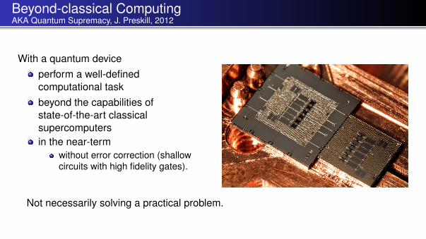
Beyond-classical ComputingAKA Quantum Supremacy, J. Preskill, 2012

With a quantum deviceperform a well-definedcomputational taskbeyond the capabilities ofstate-of-the-art classicalsupercomputersin the near-term

without error correction (shallowcircuits with high fidelity gates).

Not necessarily solving a practical problem.

Beyond-classical computing in the near-term

We want a computational task which requires direct simulation of quantumevolution.

Cost exponential in number of qubits.Typical of chaotic systems (no shortcuts).

Specific figure of merit for the computational task, related to fidelity.Relation to Computational Complexity.

Previous work in sampling problems, such as BosonSampling (Aaronson andArkhipov) and Commuting Circuits (M. Bremner et. al.).Recent conjecture by Aaronson and Chen: for a random circuit C of depth ∼ √nthere is no polynomial-time classical algorithm that guesses if | 〈0n|C |0n〉 |2 isgreater than the mediam of | 〈x |C |0n〉 |2 with success probability 1/2 + Ω(1/2n).Nevertheless, formal Computational Complexity is asymptotic, requires errorcorrection (Strong Church-Turing Thesis). We don’t know how to satisfy theprevious conjecture in the near term.

Random Universal Quantum Circuits

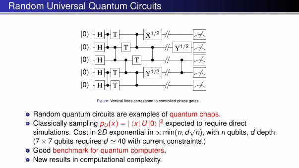
|0〉 H • T • X1/2 //

|0〉 H • • T • • // Y1/2

|0〉 H • • T • // •|0〉 H • T • • Y1/2 // •|0〉 H • T • //

Figure: Vertical lines correspond to controlled-phase gates .

Random quantum circuits are examples of quantum chaos.Classically sampling pU(x) = | 〈x |U |0〉 |2 expected to require directsimulations. Cost in 2D exponential in ∝ min(n,d

√n), with n qubits, d depth.

(7× 7 qubits requires d ' 40 with current constraints.)Good benchmark for quantum computers.New results in computational complexity.

Porter-Thomas distribution

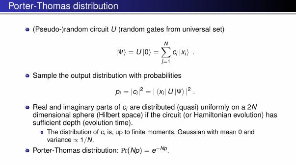
(Pseudo-)random circuit U (random gates from universal set)

|Ψ〉 = U |0〉 =N∑

j=1

ci |xi〉 .

Sample the output distribution with probabilities

pi = |ci |2 = | 〈xi |U |Ψ〉 |2 .

Real and imaginary parts of ci are distributed (quasi) uniformly on a 2Ndimensional sphere (Hilbert space) if the circuit (or Hamiltonian evolution) hassufficient depth (evolution time).

The distribution of ci is, up to finite moments, Gaussian with mean 0 andvariance ∝ 1/N.

Porter-Thomas distribution: Pr(Np) = e−Np.

Verification and uniformity test

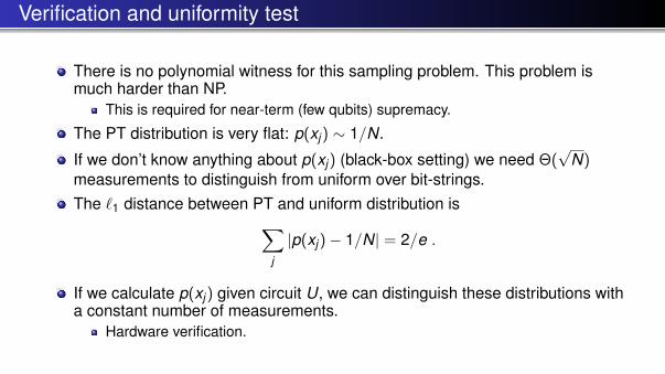
There is no polynomial witness for this sampling problem. This problem ismuch harder than NP.

This is required for near-term (few qubits) supremacy.

The PT distribution is very flat: p(xj) ∼ 1/N.

If we don’t know anything about p(xj) (black-box setting) we need Θ(√

N)measurements to distinguish from uniform over bit-strings.The `1 distance between PT and uniform distribution is∑

j

|p(xj)− 1/N| = 2/e .

If we calculate p(xj) given circuit U, we can distinguish these distributions witha constant number of measurements.

Hardware verification.

Convergence to chaos (Porter-Thomas distribution)

0 5 10 15 20 25 30

Depth

26.0

26.5

27.0

27.5

28.0

28.5

29.0

29.5

Ent

ropy

0 5 10 15 20 25 3022.5

23.0

23.5

24.0

24.5

25.0

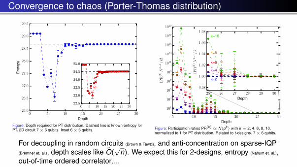
Figure: Depth required for PT distribution. Dashed line is known entropy forPT. 2D circuit 7× 6 qubits. Inset 6× 6 qubits.

5 10 15 20 25 30

Depth

101

103

105

107

109

1011

1013

1015

1017

1019

IPR

(k)Nk−

1/k

!

25 26 27 28 29 30

Depth

0.98

1.00

1.02

1.04

1.06

1.08

IPR

(k)Nk−

1/k

!

k=2

k=4

k=6

k=8

k=10

Figure: Participation ratios PR(k) ' N〈pk 〉 with k = 2, 4, 6, 8, 10,normalized to 1 for PT distribution. Related to t-designs. 7× 6 qubits.

For decoupling in random circuits (Brown & Fawzi), and anti-concentration on sparse-IQP(Bremner et. al.), depth scales like O(

√n). We expect this for 2-designs, entropy (Nahum et. al.),

out-of-time ordered correlator,...

Sampling from ideal circuit U

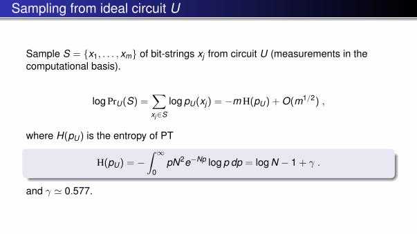
Sample S = x1, . . . , xm of bit-strings xj from circuit U (measurements in thecomputational basis).

log PrU(S) =∑xj∈S

log pU(xj) = −m H(pU) + O(m1/2) ,

where H(pU) is the entropy of PT

H(pU) = −∫ ∞

0pN2e−Np log p dp = log N − 1 + γ .

and γ ' 0.577.

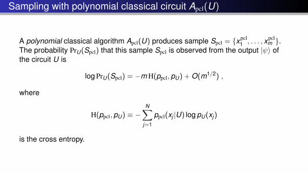
Sampling with polynomial classical circuit Apcl(U)

A polynomial classical algorithm Apcl(U) produces sample Spcl = xpcl1 , . . . , xpcl

m .The probability PrU(Spcl) that this sample Spcl is observed from the output |ψ〉 ofthe circuit U is

log PrU(Spcl) = −m H(ppcl,pU) + O(m1/2) ,

where

H(ppcl,pU) ≡ −N∑

j=1

ppcl(xj |U) log pU(xj)

is the cross entropy.

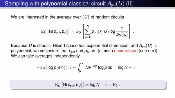
Sampling with polynomial classical circuit Apcl(U) (II)

We are interested in the average over U of random circuits

EU[H(ppcl,pU)

]= EU

N∑j=1

ppcl(xj |U) log1

pU(xj)

.

Because U is chaotic, Hilbert space has exponential dimension, and Apcl(U) ispolynomial, we conjecture that ppcl and pU are (almost) uncorrelated (see next).We can take averages independently.

−EU[log pU(xj)

]≈ −

∫ ∞0

Ne−Np log p dp = log N + γ .

EU[H(ppcl,pU)

]= log N + γ ≡ H0 .

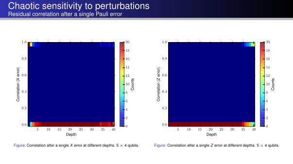
Chaotic sensitivity to perturbationsResidual correlation after a single Pauli error

5 10 15 20 25 30 35 40

Depth

0.0

0.2

0.4

0.6

0.8

1.0

Cor

rela

tion

(Xer

ror)

0

2

4

6

8

10

12

14

16

18

20

Cou

nts

Figure: Correlation after a single X error at different depths. 5× 4 qubits.

5 10 15 20 25 30 35 40

Depth

0.0

0.2

0.4

0.6

0.8

1.0

Cor

rela

tion

(Zer

ror)

0

2

4

6

8

10

12

14

16

18

20

Cou

nts

Figure: Correlation after a single Z error at different depths. 5× 4 qubits.

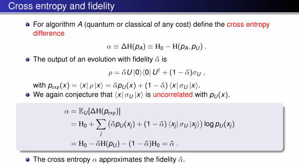
Cross entropy and fidelity

For algorithm A (quantum or classical of any cost) define the cross entropydifference

α ≡ ∆H(pA) ≡ H0 − H(pA,pU) .

The output of an evolution with fidelity α is

ρ = αU |0〉〈0|U† + (1− α)σU ,

with pexp(x) = 〈x | ρ |x〉 = αpU(x) + (1− α) 〈x |σU |x〉.We again conjecture that 〈x |σU |x〉 is uncorrelated with pU(x).

α = EU [∆H(pexp)]

= H0 +∑

j

(αpU(xj) + (1− α) 〈xj |σU |xj〉

)log pU(xj)

= H0 − αH(pU)− (1− α)H0 = α .

The cross entropy α approximates the fidelity α.

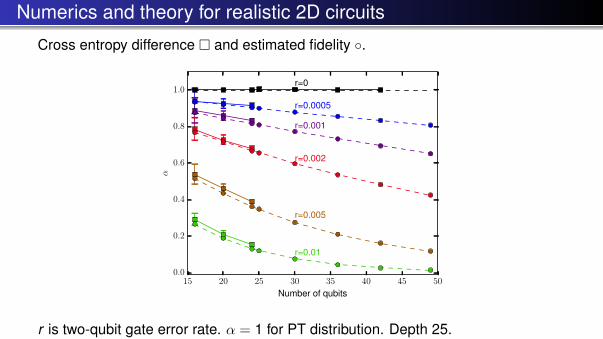
Numerics and theory for realistic 2D circuits

Cross entropy difference and estimated fidelity .

15 20 25 30 35 40 45 50

Number of qubits

0.0

0.2

0.4

0.6

0.8

1.0

α

r=0.0005

r=0.001

r=0.002

r=0.005

r=0.01

r=0

r is two-qubit gate error rate. α = 1 for PT distribution. Depth 25.

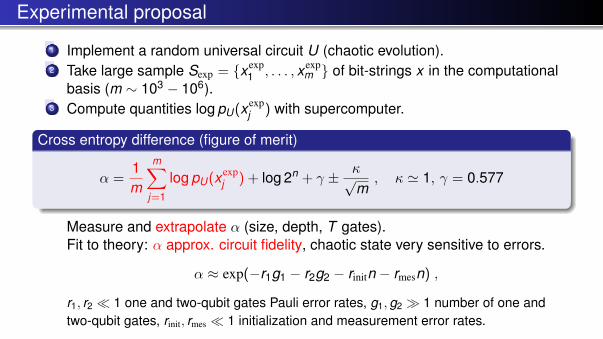
Experimental proposal

1 Implement a random universal circuit U (chaotic evolution).2 Take large sample Sexp = xexp

1 , . . . , xexpm of bit-strings x in the computational

basis (m ∼ 103 − 106).3 Compute quantities log pU(xexp

j ) with supercomputer.

Cross entropy difference (figure of merit)

α =1m

m∑j=1

log pU(xexpj ) + log 2n + γ ± κ√

m, κ ' 1, γ = 0.577

Measure and extrapolate α (size, depth, T gates).Fit to theory: α approx. circuit fidelity, chaotic state very sensitive to errors.

α ≈ exp(−r1g1 − r2g2 − rinitn − rmesn) ,

r1, r2 1 one and two-qubit gates Pauli error rates, g1,g2 1 number of one andtwo-qubit gates, rinit, rmes 1 initialization and measurement error rates.

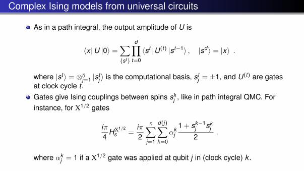
Complex Ising models from universal circuits

As in a path integral, the output amplitude of U is

〈x |U |0〉 =∑st

d∏t=0

〈st |U(t) |st−1〉 , |sd〉 = |x〉 .

where |st〉 = ⊗nj=1 |st

j 〉 is the computational basis, stj = ±1, and U(t) are gates

at clock cycle t .Gates give Ising couplings between spins sk

j , like in path integral QMC. Forinstance, for X1/2 gates

iπ4

HX1/2

s =iπ2

n∑j=1

d(j)∑k=0

αkj

1 + sk−1j sk

j

2.

where αkj = 1 if a X1/2 gate was applied at qubit j in (clock cycle) k .

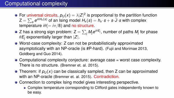
Computational complexity

For universal circuits, pU(x) = λ|Z |2 is proportional to the partition functionZ =

∑s eiθHx (s) of an Ising model Hx (s) = hx ·s + s ·J ·s with complex

temperature iθ(= iπ/8) and no structure.Z has a strong sign problem: Z =

∑j MjeiθEj , number of paths Mj for phase

θEj exponentially larger than |Z |.Worst-case complexity: Z can not be probabilistically approximatedasymptotically with an NP-oracle (is #P-hard). (Fujii and Morimae 2013,Goldberg and Guo 2014).Computational complexity conjecture: average case = worst case complexity.There is no structure. (Bremner et. al. 2015).Theorem: if pU(x) can be classically sampled, then Z can be approximatedwith an NP-oracle (Bremner et. al. 2015). Contradiction.Connection to complex Ising model gives interesting perspective.

Complex temperature corresponding to Clifford gates independently known tobe easy.

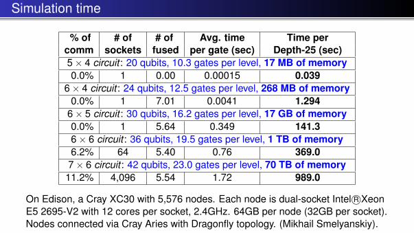
Simulation time

% of # of # of Avg. time Time percomm sockets fused per gate (sec) Depth-25 (sec)5× 4 circuit : 20 qubits, 10.3 gates per level, 17 MB of memory0.0% 1 0.00 0.00015 0.039

6× 4 circuit : 24 qubits, 12.5 gates per level, 268 MB of memory0.0% 1 7.01 0.0041 1.294

6× 5 circuit : 30 qubits, 16.2 gates per level, 17 GB of memory0.0% 1 5.64 0.349 141.36× 6 circuit : 36 qubits, 19.5 gates per level, 1 TB of memory6.2% 64 5.40 0.76 369.07× 6 circuit : 42 qubits, 23.0 gates per level, 70 TB of memory

11.2% 4,096 5.54 1.72 989.0

On Edison, a Cray XC30 with 5,576 nodes. Each node is dual-socket Intel R©XeonE5 2695-V2 with 12 cores per socket, 2.4GHz. 64GB per node (32GB per socket).Nodes connected via Cray Aries with Dragonfly topology. (Mikhail Smelyanskiy).

Some open questions

Practical computations with near-term small low-depth high-fidelity quantumcircuits. Details matter.

Quantum chemistry.Approximate optimization.

Experimental proof of error-correction.Solve the control problem (see, i.e., D-Wave).Improve fidelity (coherent and incoherent errors).Complexity theory without full error correction. (Bremner et. al.arXiv:1610.01808.)

Improve bounds in 2D random circuits: anti-concentration, t-designs,complexity bounds.Optimal classical-simulation algorithms. Details matter.

Conclusions

We expect to be able to approximately sample the output distribution ofshallow random circuits of 7× 7 qubits with significant fidelity in the near term.We don’t know how to approximately sample the output distribution of shallowrandom quantum circuits of ≈ 48 qubits with state-of-the-art supercomputers(d ∼ 40).Beyond-classical computing.New method to benchmark complex quantum circuits efficiently.Relation to computational complexity.The cross entropy method applies to other sampling problems: chaoticHamiltonians, commuting quantum circuits.

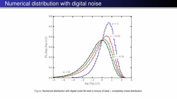
Numerical distribution with digital noise

−5 −4 −3 −2 −1 0 1 2 3

log (NpU(x))

0.0

0.1

0.2

0.3

0.4

0.5

0.6

Pr α

(log

(Np U

(x))

)

α = 1

α = 0.43

α = 0.18

α = 0

Figure: Numerical distribution with digital noise fits well a mixture of ideal + completely mixed distribution.

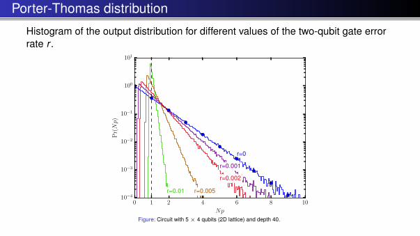
Porter-Thomas distribution

Histogram of the output distribution for different values of the two-qubit gate errorrate r .

0 1 2 4 6 8 10

Np

10−4

10−3

10−2

10−1

100

101

Pr(Np)

r=0

r=0.001

r=0.002

r=0.005r=0.01

Figure: Circuit with 5× 4 qubits (2D lattice) and depth 40.

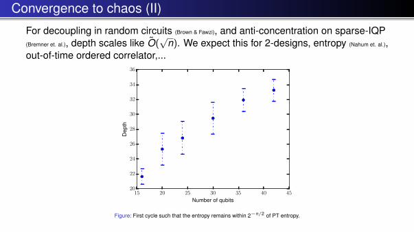
Convergence to chaos (II)

For decoupling in random circuits (Brown & Fawzi), and anti-concentration on sparse-IQP(Bremner et. al.), depth scales like O(

√n). We expect this for 2-designs, entropy (Nahum et. al.),

out-of-time ordered correlator,...

15 20 25 30 35 40 45

Number of qubits

20

22

24

26

28

30

32

34

36

Dep

th

Figure: First cycle such that the entropy remains within 2−n/2 of PT entropy.