Embed Size (px)
Citation preview
I
CHARACTERIZATION OF T H E COOLING AND
TRANSFORMATION OF STEELS O N A
RUN-OUT T A B L E OF A HOT-STRIP M I L L
By
CRAIG A L L E N M C C U L L O C H
B.A.Sc, The University of British Columbia, 1986
A THESIS SUBMITTED IN PARTIAL F U L F I L L M E N T OF
T H E REQUIREMENTS FOR T H E D E G R E E O F
MASTER OF APPLIED SCIENCE
in
T H E F A C U L T Y OF G R A D U A T E STUDIES
M E T A L S A N D MATERIALS ENGINEERING
We accept this thesis as confonning to the required standard
T H E UNIVERSITY OF BRITISH COLUMBIA August 1988
©Craig Allen McCulloch, 1988

In presenting this thesis in partial fulfilment of the requirements for an advanced
degree at the University of British Columbia, I agree that the Library shall make it
freely available for reference and study. I further agree that permission for extensive
copying of this thesis for scholarly purposes may be granted by the head of my
department or by his or her representatives. It is understood that copying or
publication of this thesis for financial gain shall not be allowed without my written
permission.
Department of M e t a l s a n d M a t e r i a l s E n q i n e e r i n g
The University of British Columbia 1956 Main Mall Vancouver, Canada V6T 1Y3
DE-6(3/81)

A B S T R A C T
A mathematical model has been developed to predict the thermal history of strip
during cooling on the run-out table of a hot strip mill. The model incorporates phase
transformation kinetics and accounts for the heat of transformation. To characterize the
cooling by laminar water sprays, in-plant trials were conducted at the Stelco Lake Erie
Works hot strip mill. The temperature data was used in the thermal model to calculate
an overall heat transfer coefficient for a laminar water bank of 1 kW/m 2 , C. Isothermal
diametral dilatometer testing was used to generate phase transformation kinetics for a
0.34 weight percent plain carbon steel. Continuous cooling dilatometer testing was
used to calculate the transformation start time as a function of the cooling rate. The
high cooling rates of 40 *C/s to 50*C/s, experienced on the run-out table had the effect
of depressing the transformation start temperature by over 100'C.
The phase transformation kinetics were incorporated in a phase transformation model
and employed to predict thermal profiles for a 0.34 carbon plain-carbon steel. The
temperature predictions were within 25"C of the plant pyrometer readings using the
calculated overall heat transfer coefficient and within 35°C of the plant pyrometer
values using literature derived heat transfer coefficients.
A simulation of the model predicted cooling conditions on a Gleeble high
temperature testing machine showed that the transformation was occurring at
approximately 730*C. The empirical transformation start time, obtained from cooling
ii

rate versus transformation start time tests, which was used in the phase transformation
portion of the model, and the Gleeble simulation gave excellent agreement with the
model thermal profile predictions.
iii

T A B L E OF CONTENTS
Abstract ii
Table of Contents iv
List of Tables viii
List of Figures ix
Acknowledgment xvi
1.0 INTRODUCTION 1
2.0 LITERATURE REVIEW 3
2.1 Heat Transfer on the Run-out Table 3
2.1.1 Heat Transfer Coefficients for Water Bar and Water
Curtain Cooling from Plant Data 4
2.1.2 Heat Transfer Coefficients for Water Bar Cooling
from Experimental Measurements 5
2.1.3 Heat Transfer Coefficient for Roll Contact Cooling
from Experimental Measurements 9
2.2 Phase Transformation Kinetics 10
2.3 Review of Related Models , 13
2.4 Figures 16
3.0 SCOPE A N D OBJECTTVES 17
3.1 Scope 17
3.2 Objectives 18
4.0 PROCEDURE 19
iv
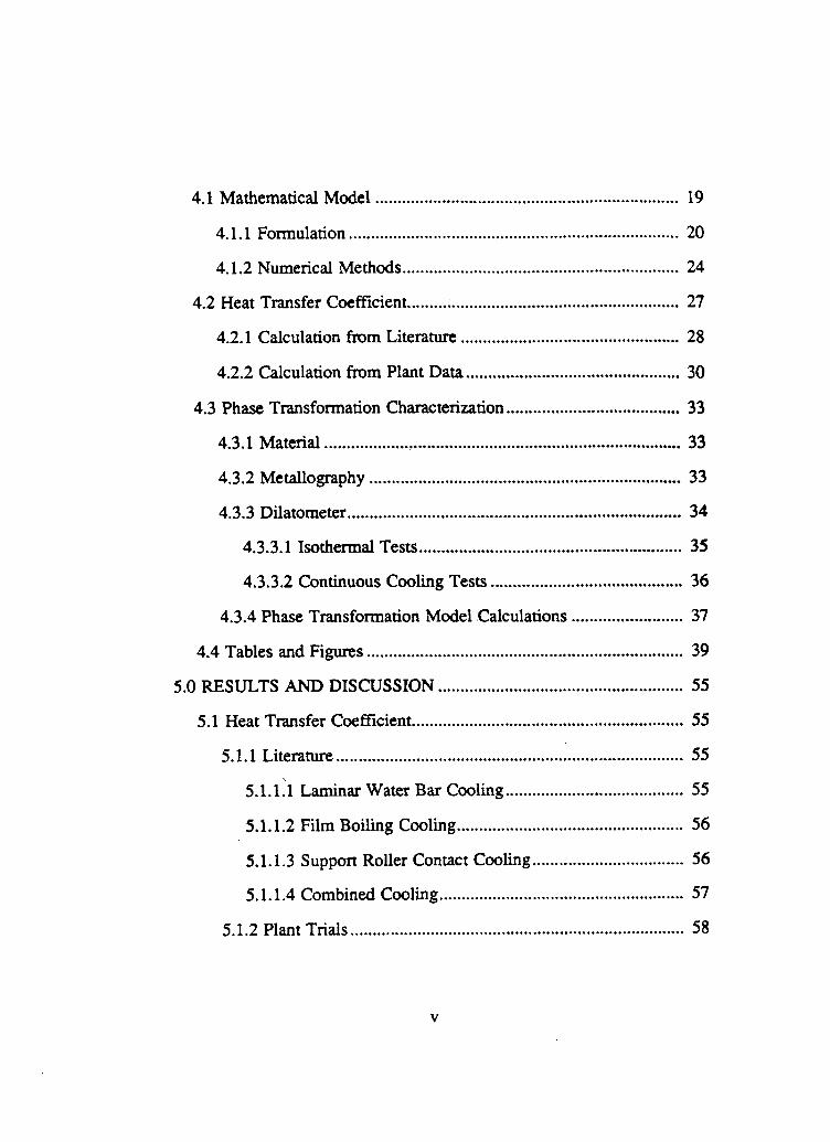
4.1 Mathematical Model 19
4.1.1 Formulation 20
4.1.2 Numerical Methods 24
4.2 Heat Transfer Coefficient 27
4.2.1 Calculation from Literature 28
4.2.2 Calculation from Plant Data 30
4.3 Phase Transformation Characterization 33
4.3.1 Material 33
4.3.2 Metallography 33
4.3.3 Dilatometer 34
4.3.3.1 Isothermal Tests 35
4.3.3.2 Continuous Cooling Tests 36
4.3.4 Phase Transformation Model Calculations 37
4.4 Tables and Figures 39
5.0 RESULTS A N D DISCUSSION 55
5.1 Heat Transfer Coefficient 55
5.1.1 Literature 55
5.1.1.1 Laminar Water Bar Cooling 55
5.1.1.2 Film Boiling Cooling 56
5.1.1.3 Support Roller Contact Cooling 56
5.1.1.4 Combined Cooling 57
5.1.2 Plant Trials 58
v

5.1.2.1 Overall Heat Transfer Coefficient 59
5.1.2.1.1 Calculation 59
5.1.2.1.2 Sensitivity 60
5.1.2.2 Individual Heat Transfer Coefficient 62
5.2 Phase transformation 63
5.2.1 Material 63
5.2.2 Isothermal Cooling Tests 64
5.2.3 Continuous Cooling Tests 65
5.2.3.1 Metallography 66
5.2.3.2 Coiling Temperature 67
5.2.4 Model Phase Transformation Calculations 69
5.3 Mathematical Model 71
5.3.1 Sensitivity 71
5.3.2 Validation 72
5.4 Tables and Figures 73
6.0 CONCLUSIONS 133
6.1 Summary 133
6.2 Conclusions 135
6.3 Future Considerations 138
7.0 BIBLIOGRAPHY 139
8.0 APPENDIX 142
8.1 Nomenclature 142
vi

8.2 Derivation of Finite Difference Equations 145
8.2.1 Top Surface Node 145
8.2.2 Interior Nodes 146
8.2.3 Bottom Surface Node 146
8.2.4 Solution , 147
8.3 Hatta et al. Thermal Boundary Layer Calculations 147
vii

LIST OF TABLES
Table I Composition for the three steel chemistries used. 39
Table IIa....Plant conditions for four runs 73
Table Ho....Plant conditions for four runs 74
Table IIc....Plant conditions for four runs 75
Table IJJ Industrial plant cooling conditions 76
Table IV Metaliographic data for the 0.34 carbon samples, for the
down-coiler sample.the continuous cooling samples, and the Gleeble
simulation sample; with tabulated values for, cooling rate, fraction ferrite,
undercooling, and average austenite grain size 77
Table V Comparison of the composition of the down-coiler and transfer bar
medium carbon samples 78
Table VI....Grain size versus coiling temperature for 0.054 weight percent
carbon grade steel 79
Table VH....Tabulated model predictions, for low (7'C/s) and high (45'C/s)
cooling rates, and for the literature heat transfer coefficients at an average
cooling rate, (26'C/s) 80
viii

LIST OF FIGURES
Figure 1 Specific Heat as a Function of Temperature for five carbon levels,
BISRA 16
Figure 2 Hot-strip geometry used for the model 40
Figure 3 Schematic of the STELCO Lake Erie Works Hot Strip Mill
Run-out Table 41
Figure 4 Specific Heat as a Function of Temperature for a 0.34 % carbon
steel, BISRA, w/o phase transformation 42
Figure 5 Thermal Conductivity as a Function of Temperature for a 0.06 %
plain carbon steel, BISRA 43
Figure 6 Thermal Conductivity as a Function of Temperature for a 0.08 %
plain carbon steel, BISRA 44
Figure 7 Thermal Conductivity as a Function of Temperature for a 0.23 %
plain carbon steel, BISRA 45
Figure 8 Thermal Conductivity as a Function of Temperature for a 0.34 %
plain carbon steel, BISRA 46
Figure 9 Flow chart for the basic program 47
Figure 10 The six types of cooling regime experienced by the steel strip 48
Figure 11 The various film boiling heat transfer coefficients from Kokada et
al.[6] for three cooling water temperatures with two values from the
Berensen[24] horizontal surface boiling equation 49
Figure 12 Experimental verification of TAC3 and TAC1 50
ix

Figure 13 A typical dilation versus time plot for an isothermal dilatometer
test 51
Figure 14 A typical dilation and temperature versus time plot showing
transformation start and finish times 52
Figure 15 Experimental dilation and thermal dilation plots, used with
divergence method (Campbell[27]) for calculation of transformation start 53
Figure 16 Flow sheet for the iterative solution of the Avrami fraction
transformed equation as a function of temperature 54
Figure 17 Black zone radius as a function of a constant steel surface
temperature 81
Figure 18 Hatta laminar water bar heat transfer coefficient as a function of
contact radius 82
Figure 19 Thermal profile model sensitivity to changes in the water
temperature for the Kokada film boiling heat transfer coefficient 83
Figure 20 Thermal profile model sensitivity to changes in the support roller
conduction cooling 84
Figure 21 Thermal profile model literature heat transfer coefficients 0.05%
carbon, 3.89 mm gauge, target coiling temperature 720*C 85
Figure 22 Thermal profile model literature heat transfer coefficients, 0.05%
carbon, 2.62 mm gauge, target coiling temperature 720*C 86
Figure 23 Thermal profile model literature heat transfer coefficients, 0.07%
carbon, 0.024% Nb, 3.89 mm gauge, target coiling temperature 720° C 87
x

Figure 24 Thermal profile model literature heat transfer coefficients, 0.07%
carbon, 0.024% Nb, 2.62 mm gauge, target coiling temperature 720°C 88
Figure 25 Thermal profile model literature heat transfer coefficients, 0.05%
carbon, 2.62 mm gauge, target coiling temperature 620"C 89
Figure 26 A sample temperature profile from the plant data. 90
Figure 27 Thermal profile model, overall heat transfer coefficient calculated
from plant pyrometer measurements, 0.05% carbon, 3.89 mm gauge, target
coiling temperature 720"C 91
Figure 28 Thermal profile model, overall heat transfer coefficient calculated
from plant pyrometer measurements, 0.07% carbon, 0.024% Nb, 3.89 mm
gauge, target coiling temperature 720'C 92
Figure 29 Thermal profile model, overall heat transfer coefficient calculated
from plant pyrometer measurements, 0.07% carbon, 0.024% Nb, 2.62 mm
gauge, target coiling temperature 720*C 93
Figure 30 Thermal profile model, overall heat transfer coefficient calculated
from plant pyrometer measurements, 0.05% carbon, 2.62 mm gauge, target
coiling temperature 720*C 94
Figure 31 Thermal profile model, overall heat transfer coefficient calculated
from plant pyrometer measurements, 0.05% carbon, 3.89 mm gauge, target
coiling temperature 620"C 95
Figure 32 Thermal profile model, overall heat transfer coefficient calculated
from plant pyrometer measurements, 0.05% carbon, 3.89 mm gauge, target
xi

coiling temperature 540°C 96
Figure 33 Thermal profile model sensitivity, overall heat transfer coefficient
calculated from plant pyrometer measurements, 0.05% carbon, 3.89 mm gauge,
target coiling temperature 720°C 97
Figure 34 Thermal profile model sensitivity, individual laminar water bar
heat transfer coefficient, 10 kW/m 2 ,C with 20 kW/m2 ,C and 5 kW/m2 oC
deviations,target coiling temperature 720*C 98
Figure 35 Isothermal dilatometer results for 673*C test, dilation-time and
temperature-time 99
Figure 36 AD/AT as a function of time for the 673'C isothermal test 100
Figure 37 Isothermal dilatometer test sample plot lnln(l/(l-FX)) vs ln(t) for
673"C fraction ferrite transformed 101
Figure 38 ln(b) Avrami coefficient for the isothermal formation of ferrite in
the 0.34 carbon steel 102
Figure 39 ln(b) Avrami coefficient for the isothermal formation of pearlite in
the 0.34 carbon steel 103
Figure 40 Avrami coefficient, nf, for the austenite-to-ferrite transformation in
the 0.34 % C, plain carbon steel 104
Figure 41 Avrami coefficient, n,,, for the austenite-to-pearlite transformation
in the 0.34 % C, plain carbon steel 105
Figure 42 Calculated ln(b) values for the ferrite transformation assuming n<=
1.25, for 0.34% carbon steel 106
xii
Figure 43 Calculated ln(b) values for the pearlite transformation assuming Ap
= 1.14, for 0.34% carbon steel 107
Figure 44 Average Avrami coefficient V for 0.34% carbon compared to
other experimental values (Campbell[27]) 108
Figure 45 Comparison of the ln(b) Avrami coefficient for the
austenite-ferrite transformation in several plain-carbon steels(Campbell[27]) 109
Figure 46 Comparison of the ln(b) Avrami coefficient for the
austenite-pearlite transformation in several plain-carbon steels(Campbell[27])... 110
Figure 47 Temperature as a function of time for a continuous cooling rate of
27'C/s I l l
Figure 48 Thermal and Experimental dilatometer values as a function of
time for a cooling rate of 27*C/s 112
Figure 49 The undercooling for the austenite-to-ferrite start temperature as a
function of cooUng rate 113
Figure 50 Fraction ferrite as a function of cooling rate, from metallographic
examination 114
Figure 51 Continuously cooled dilatometer sample 115
Figure 52 Continuously cooled dilatometer sample showing banding 116
Figure 53 Medium carbon down-coiler sample 117
Figure 54 Surface thermal profile, using the overall heat transfer coefficient,
1 kW/m 2 , C, Table rn run one cooling conditions, and a transformation start
temperature of 732'C (dT/dt = 7°C/s) 118
xiii

Figure 55 Surface thermal profile, using the overall heat transfer coefficient,
1 kW/m 2 o C, Table in run two cooling conditions, and a transformation start
temperature of 732'C (dT/dt = TCJs) 119
Figure 56 Surface thermal profile, using the overall heat transfer coefficient,
1 kW/m 2 °C, Table LTI run three cooling conditions, and a transformation start
temperature of 732'C (dT/dt = 7'C/s) 120
Figure 57 Surface thermal profile, using the overall heat transfer coefficient,
1 kW/m 2*C, Table DI run one cooling conditions, and a transformation start
temperature of 688'C (dT/dt = 45'C/s) 121
Figure 58 Surface thermal profile, using the overall heat transfer coefficient,
1 kW/m 2*C, Table in run two cooling conditions, and a transformation start
temperature of 688'C (dT/dt = 45'C/s) 122
Figure 59 Surface thermal profile, using the overall heat transfer coefficient,
1 kW/m2"C, Table DI run three cooling conditions, and a transformation start
temperature of 688'C (dT/dt = 45'C/s) 123
Figure 60 Surface thermal profile, using the literature heat transfer
coefficients, Table DI run one cooling conditions, and a transformation start
temperature of 710"C (dT/dt = 26'C/s) 124
Figure 61 Surface thermal profile, using the literature heat transfer
coefficients, Table DI run two cooling conditions, and a transformation start
temperature of 710'C (dT/dt = 26'C/s) 125
Figure 62.....Surface thermal profile, using the literature heat transfer
xiv
coefficients, Table DJ run three cooling conditions, and a transformation start
temperature of 710*C (dT/dt = 26'C/s) 126
Figure 63 Effect on predicted center line temperature of changes in the
number of nodes through thickness 127
Figure 64 Effect on predicted center line temperature of changes in the step
size, where the step size equals the strip velocity times the time increment 128
Figure 65 Effect of the ±0.3m/s deviation of the strip velocity on the
predicted temperature profile 129
Figure 66 Industrial cooling profile simulated on the Gleeble high
temperature testing machine 130
Figure 67 Industrial cooling conditions, simulated on a Gleeble high
temperature testing machine 131
Figure 68 Microstructure of the Gleeble cooling simulation sample for the
Table HI run one cooling conditions 132
xv

Acknowledgment
I would like to acknowledge the support provided for this project by NSERC and
Stelco Inc. The guidance of my thesis supervisors I.V. Samarasekera and E.B. Hawbolt
is also much appreciated. On the experimental side, Keith Barnes, Henk Averink, and
Barbara Zbinden were of major assistance in securing the industrial temperature data as
was Bihn Chau with the dilatometer phase transformation kinetics.
xvi

INTRODUCTION 1
1 INTRODUCTION
Historically the production of flat rolled product has been based on previous experi
ence. New materials or new physical properties for existing materials, were produced by
a trial and error process by examining the effects of minor modifications to the
rolhng/ccoling conditions. The introduction of the computer to industrial applications
initially changed the experience reservoir from the on-line staff to the machine, with little
modification of the trial and error methods historically used.
Approximately one half of the finished steel in North America is in the form of
sheet or strip, with hot rolled strip being used in a wide variety of applications ranging
from auto body to the shells of stoves and refrigerators. Furthermore, there has been a
proliferation of non ferrous products in the market place of lightweight materials with
mechanical properties equivalent to those of steel. The steel industry has responded by
developing lighter gauge steel to lower the weight without an attendant loss of strength.
To produce a strip steel of improved physical properties with decreased weight the vari
ables in the process must be well controlled; the final overall physical properties are
affected by the chemical composition and thermo-mechanical history of the steel. Thus,
the initial composition of the steel, the casting and reheating processes, together with the
thermo-mechanical history of the steel during rolling and subsequent cooling profoundly
influences the final mechanical properties of the strip.
The economic down-tum at the start of this decade emphasized the need for tighter
control of the hot rolling process to minimize costs. The use of niobium-titanium-
1

INTRODUCTION 1
vanadium additives for increased strength became routine, although mill scheduling was
accomplished by trial and error. Hot strip mills world wide are now controlled by
empirical or semi-empirical computer models with some operator input, but, a better
thenno-mechanical understanding of the entire rolling mill is needed in order to produce
control models that decrease deviations from target physical properties.
The rolling mill and the run-out table have been modeled from both an experimen-
tal(empirical) and a theoretical(mathematical) point of view in an effort to provide better
mill operational control. Mathematical models of these processes are also being
developed in order to provide a better understanding of the theoretical aspects of thermo-
mechanical processing of steel. One area that is not well understood is the relationship
between the process variables and the transformation from austenite to ferrite/pearlite
during run-out table cooling. The phase transformation effects have historically been
included in models by incorporating a specific heat value that includes the recalescence
due to phase transformation, however, the cooling rate strongly influences the start of
transformation and thus kinetics must be considered in any modeling effort.
The object of this thesis was to model the temperature and microstructure of the
hot-strip as it passes along the run-out table from exit of the finishing stands until
entrance to the pinch roller of the down-coiler. A better understanding of the heat trans
fer to the cooling water sprays and of the kinetics of the phase transformation was sought
in an attempt to provide a realistic model of the process.
2

LrTERATURE REVIEW 2.1
2 LITERATURE REVIEW The current literature on hot strip run-out table cooling covers all aspects of the
process. These range from a description of new cooling techniques to composition
control for the production of steels with improved mechanical properties. They also
include reviews of models for process control. Of particular interest to this thesis are
measurements of or expressions quantifying the heat transfer between the strip and
cooling water on the run-out table, phase transformation kinetics under non-equilibrium
conditions and mathematical models coupling the two phenomena.
2.1 Heat Transfer on the Run-Out Table
On the run-out table the strip is cooled by a laminar water bar or water curtain. The
former technique has received its name because of the 'glassy' or 'rod-like' non-turbulent
appearance rather than due to a strict Reynolds number definition of laminar flow. A
water curtain has been described as a continuous water bar in that it resembles a laminar
sheet or 'curtain' of water. Cooling occurs by forced convection in the zone of direct
contact and by film boiling across a vapour barrier in the region surrounding the impact
zone. The heat transfer coefficient for laminar water bar, water curtain, and film boiling
may be determined empirically from in-plant temperature measurements or from
laboratory experiments. Heat is also transferred to the support rolls by conduction and to
the surrounding air by radiation.
3

LITERATURE REVIEW 2.1.1
2.1.1 Heat Transfer Coefficients for Water Bar and Water
Curtain Cooling from Plant Data
In this approach heat transfer coefficients are back calculated from in-plant strip
surface temperature measurements. Tacke et al.[l] studied the two types of water cooling
as well as the spray nozzle cooling previously employed on run-out tables. To a run-out
table with a standard spray nozzle header configuration, they added a bank of laminar
water bar headers and a bank of water curtain headers . Each cooling bank had a
blow-off and a pyrometer mounted before and after the bank to give an accurate reading
of surface temperature. Using the measured temperature changes across a cooling bank
in a finite element model they calculated an overall heat transfer coefficient for each type
of cooling bank as a function of the water application rate. From this they derived values
of 1800 W / m 2 , C ± 2 0 0 W / m 2 , C for the bank of water curtain cooling, 1300 W/m2*C ±200
W/m 2 o C for the bank of laminar water bar cooling, and 900 W/m 2 o C ±150 W / m 2 , C for the
bank of spray nozzle cooling. While the water curtain cooling had the highest heat
transfer coefficient, the water application was uneven over the strip. The laminar water
bar gave an even water application over the full strip width and so was chosen for plant
use even thoygh the resultant heat transfer coefficient was less than that for water curtain
cooling. They report cooling rates of 50°C/s up to 200°C/s depending on strip gauge with
laminar water bar cooling. They also report that front end loading the cooling, that is
using water sprays at the finish mill end of the run-out table resulted in an increase in
yield strength over tail end loading, cooling with the sprays at the down-coiler end of the
4

LITERATURE REVIEW 2.1.2
run-out table. They note that in a series of over seven hundred strips using the laminar
water bar cooling coupled with the calculated heat transfer coefficients in their plant
control model the two sigma deviation was reduced from an average value of 45°C down
to 20'C.
Colds and Sellars[2] have calculated a heat transfer coefficient for an individual
water curtain by using a finite difference heat transfer model with various values included
for water curtain and film boiling cooling. The resulting thermal profile is compared to
observed values to arrive at a result of 17 kW/m 2 , C for an individual water curtain; they
comment on the difficulty in producing an exact value due to the short residence time of
the strip under the water curtain contact area which they assume to have a diameter of
two to three times the water curtain diameter. They use a film boiling cooling heat
transfer value of 150 W/m2"C for the region outside the contact zone which compares
well with the Farber and Scorah[3] value of between 150 W / m 2 , C and 170 W/m 2 o C.
2.1.2 Heat Transfer Coefficients for Water Bar Cooling from
Experimental Measurements
Individual laminar water bar heat transfer coefficients and values for the associated
film boiling cooling in the surrounding region were presented in three articles by
Hatta[5,6], Kokada[7], et al. The Hatta et al. results were based on an examination of the
cooling associated with a single laminar water bar over a stationary 10 mm thick stainless
steel plate with low water flow rates. The plate was instrumented with five
thermocouples inserted from the back of the plate at a depth of 8 mm from the top surface
5

LITERATURE REVIEW 2.1.2
at 20 mm increments from the water bar contact center line. The plate was heated in a
reducing furnace to hot-strip temperatures, it was then removed and placed under a
laminar water bar header. The temperature change over time for various water
temperature and flow rates was recorded. This data was then used in a finite difference
model to derive an equation for a heat transfer coefficient. A heat transfer coefficient of
15.93 W/m 2"C was adopted for natural convection in air in the Hatta model.
The Hatta et al. experiments produced a number of general observations about the
water cooling under a laminar water bar. First, that there is a 'black zone' around the
area under the water bar which did not show any boiling phenomena. Second, around
this 'black zone' was an area of film boiling. Third, the transition between the boiling
and non-boiling areas appeared to be instantaneous; that is, there did not appear to be a
visible transition cooling regime. Using these observations and the data produced from
the thermocouples, a heat transfer coefficient equation was obtained,
. . . 1
where 0.063 is an experimentally derived constant
k is the thermal conductivity of the water, in W/mK
r is the laminar water bar contact radius, in meters
Re is the Reynolds number
and Pr is the Prandd number
The heat transfer coefficient for the film boiling region is,
6

LITERATURE REVIEW 2.1.2
a™ = 200* 2420-21.70V) . . . 2
,•8
where T w is the average water temperature, in Kelvin
T s is the steel temperature, in Kelvin
and T S A X is the saturation temperature of the water, in Kelvin.
The water saturation temperature under one atmosphere pressure is 100 °C. The
water temperature at which the transition from water contact cooling to film boiling
cooling occurs, Tom-, is described by the equation,
The value of ranges from 18.75 "C for a steel temperature of 1000 *C to 100'C
for a steel temperature of 350 *C. Hatta, Kokada, et al. noted that film boiling was not
observed for a water temperature lower than 68 °C. The cooling water temperature, T w ,
must therefore be between the minimum critical transition temperature, Tdm- = 68 *C,
and the saturation temperature, T S A X = 100 *C. The water temperature used in the model
is a simple average of these two values,
-(7^-1150)
8
. . . 3 cm ~
1 0 0 o C + 6 8 ° C 2
= 84°C . . . 4
which is used as T w for Eq.2.
7

LITERATURE REVIEW 2.1.2
A horizontal water velocity1 is needed to derive a water film thickness as well as for
computation of the Reynolds number used in Eq.l; this is calculated based on the
assumption that the horizontal water velocity is equal to the vertical water velocity which
is determined by the water flow rate. Hatta et al. used the heat transfer coefficients
calculated in Eq. 1 and Eq.2 to calculate a thermal profile for the plate. The calculated
profiles were then compared to the thermocouple data and it was found that greater
cooling was predicted by the calculated heat transfer coefficient than was observed
experimentally. To compensate for this over cooling Hatta et al.[6] postulated that there
is a 'thermal zone' in the water film layer, not all of the water film thickness was affected
by the heat flow. The thermal zone2, a boundary layer phenomena, is the thickness of
water above the plate that is heated in a finite time period. This was used in Hatta's
model with Eq. 1 for the area under the laminar water bar and Eq.2 for the film boiling
zone to calculate a new thermal profile which gave good agreement with the
experimental results. Eq. l is insensitive to the water flow rate but relatively sensitive to
the area of contact under the laminar water bar3.
1 Equation 1 in the appendix
2 Water film thickness, described in the appendix
3 From Eq.Al in the appendix
8

LITERATURE REVIEW 2.1.3
2.1.3 Heat Transfer Coefficient for Roll Contact Cooling from
Experimental Measurements
Diener and Drastik[7] examined heat flow between guide rolls4 and continuously
cast slab using instrumented rolls and developed heat flux profiles for various cooling
types. Using their 'quasi-stationary' heat flux value of 75 kW/m with an average
temperature difference of 900 *C, an average heat transfer coefficient of 83 W/m 2 o C can
be calculated.
4 On the inside of the curve above the slab
9

LITERATURE REVIEW 2.2
2.2 Phase T rans fo rmat ion
The phase transformation and its associated heat of transformation has been
characterized with a variety of methods, the predominant one being the use of a modified
specific heat value. The specific heat values tabulated by the British Iron and Steel
Research Association, BISRA[8], include the effects of the phase change by
incorporating the heat of transformation in the specific heat value to give a greatly
increased value at the phase transformation temperature, as can be seen in Figure 1. If
the specific heat is taken as a temperature dependent value which includes the heat of
transformation, then the thermal effects of the phase transformation can be accounted for
in this way. The BISRA specific heat values were obtained from plant measurements
made in the early 1950's and do not include the modem alloys. The data range is based
only on the weight percent carbon and a variation in carbon content of 0.06 to 0.40
weight percent; individual values are an average for a 50 °C temperature range. The
BISRA values are for equilibrium and any effects of cooling rate are ignored.
The use of the isothermal kinetics to describe the continuous cooling transformation
is based on the Avrami [10] formula,
X = l-expH>r") • • • 5
where X is the fraction transformed, t is time, and b and n are two coefficients called the
'Avrami' coefficients. This is based on the additivity concept first postulated by Scheil5
in 1935. An additive system is one in which the transformation is only a function of the
5 For incubation not for phase transformation as such
10

LITERATURE REVIEW 2.2
temperature and the fraction previously transformed. In an additive system a continuous
process can be approximated as the sum of a series of discrete steps; this is very useful in
mathematical modeling. The Avrami formula presents the fraction transformed ( X ) as a
function of time (t) and the two 'Avrami' coefficients 'b' and V . Avrami[9,10,ll], and
later Cahn[12] postulated separate criterion for determining if a system is additive.
Avrami described an ' isokinetic' condition in which the ratio of nucleation and growth
rate is constant. Cahn described a site saturation criterion based on preferential
nucleation sites. Agarwal and Brimacombe[13] used the additivity concept in their
model of rod cooling, noting that while the system being examined did not satisfy either
criterion, the results from the model based on the assumption of an additive system
agreed with experimental observations. Kuban et al.[14] examined the additivity of the
austenite to pearlite transformation to determine conditions over which additivity applied.
They postulated a criterion of 'effective site saturation' based on the concept that most of
the growth of the new phase, pearlite, is growth at the initially nucleated sites with the
sites nucleated near the end of the transformation contributing very little to the overall
volume change. The effective site saturation criterion was found to be valid if the time
for twenty percent of the transformation was experimentally greater than 0.28 times the
time for ninety percent of the transformation,
r 2 0> 0.28^ . . . 6
Hawbolt et al.[15,16] examined the austenite-to-pearlite transformation for a
eutectoid steel and the austenite-to-ferrite and pearlite transformations for a 1025 steel
using a dilatometer to determine phase transformation kinetics and start temperatures.
11

LITERATURE REVIEW 2.2
The Avrami coefficients, n, and, b, were determined from isothermal tests. The
transformation start time (or temperature) and the total fraction ferrite formed as a
function of cooling rate were determined using continuous cooling tests.
A different method of dealing with the phase transformations occurring on a run-out
table was examined by Morita et al.[17]. They used an on-line transformation detector
measuring the change in magnetic resistance of the strip to determine the fraction
transformed on the run-out table. The concept of an on-line transformation detector
under the strip is potentially very desirable. However, machine calibration and data
interpretation seem dependent on trial and error. Until a theoretical model capable of
interpreting the change in magnetic resistance in terms of the kinetics of the austenite to
ferrite and ferrite plus pearlite transformation is available, the on-line transformation
detector, while sophisticated, requires substantial experimental data to describe the
transformation behavior.
12

LITERATURE REVIEW 2.3
2.3 Review of Related Models
Of the various published models pertaining to run-out table cooling of hot strip,
most are intended for use in mill control. They range from the Hinrichsen[18] dynamic
systems approach to the Hurkmans et al.[19] experimentally produced deformation
transformation model. Hinrichsen[18] modeled the run-out table as a dynamic simulation
via a systems control approach used widely in chemical engineering applications. He
formulated a dynamic model of the run-out table including the gain and dead time of each
component, from the spray water valves to the run-out table pyrometer. He then used
experimental data to tune the response of the dynamic model. The entire process is
controlled with a proportional-integral controller using modified feedback compensated
feed-forward control to prevent cumulative errors from inducing increasing oscillation.
This is a widely used control system in areas where there is small variability in the
desired output product. With hot-strip, current production requires output of many
products with different properties from the same production line, which makes this type
of model of limited utility.
A basic model used in a wide variety of plants is the basic heat transfer model as
exemplified by Tacke et al.[l]. This model is described in the preceding section A. and is
an excellent example of the use of empirical data and mathematical modeling to control
run-out table output. The heat transfer models found in the literature vary in their levels
of sophistication. These range from the simple Longenberger[20] model to the
sophisticated Tacke et al.[l] model. The Longenberger[20] one dimensional model
13

LITERATURE REVIEW 2.3
discretizes the strip through thickness into three nodes and the resulting model is tuned
through statistical regression. Miyake[21] has produced a more sophisticated model
which mathematically characterizes the losses due to radiation and water cooling but is
still fine tuned with empirical data. The Tacke et al.[l] model, previously described, uses
a finite element approach and back calculated heat transfer coefficients to produce an
on-line control model and represents the most sophisticated of the purely heat transfer
models.
More complex still are the models that add microstructural considerations to the
basic thermal model. Yada[20] uses additivity and the assumption of a transformation
rate independent of time. The entire rolling mill is approximated as a series of
independent models; one for hot deformation, resistance to hot deformation, a
temperature profile model, a transformation model based on nucleation and growth, and a
structure versus properties model. The model outputs are combined to produce a
prediction of the final microstructure and the physical properties and are used as an
on-line mill control model. The model is used on-line to compensate strip cooling for
variations in strip velocity to maintain the consistency of the strip properties. Yada notes
that some form of on-line microstructural information would be useful during processing
to eliminate cumulative errors and to this end he suggests the use of the magnetic
transformation detector described by Morita et al.[17].
The most comprehensive approach is that of Hurkmans et al.[19] in which
dilatometry is used to characterize the phase transformation kinetics for a given
chemistry. The dilatometric data for a given test is reduced to a group of between thirty
14

LITERATURE REVIEW 2.3
to sixty points which are then fitted to a cubic spline interpolation. From the interpolated
data a set of thirty data values are produced and used for all future calculations. From the
fitted data set the rate of diametral change over time and the rate of temperature change
over time is calculated. This is similar to the method used by Hawbolt et al.[15,16] but,
with the interpolation of the raw data, variations due to experimental differences between
individual data runs should be minimized. The diametral change with time data is
integrated to produce fraction transformed data. This data is then fitted to an equation by
a least squares approximation to produce values for the constants A±, B k , and Q used in,
dt
where 'az Jk
4
e
= Ak(Zk + e)%>
is the rate of transformation for phase k,
is the fraction of phase k transformed,
is the fraction of y phase transformed,
is a small number needed in integration of the
differential equation.
The constants are derived for a given phase, composition, and austenitizing
condition. Hurkmans et al.[19] have used the model for ferrite, pearlite, bainite, and
martensite transformations. This data is used in an in-plant control model and has
resulted in a reduction of overall water consumption while maintaining the desired
microstructure.
15

LITERATURE REVIEW 2.4
2.4 Figures
c o "9 v $ v O v g v O v.e(
w co CM o a o 5 d ci d ci a O) CD
5
>«r>+
-Mac
-K>
O + <
+ •
- m a x • M I X
1 1 -
(fl m CO CM T -
I 1 1 1 1 1— i - O) oo s to in ^ d d d d d ci
Specific Heat W/kg C
(X 1000)
Figure 1 Specific Heat as a Function of Temperature for five carbon levels, BISRA
16

SCOPE A N D OBJECTIVES 3.1
3 SCOPE A N D OBJECTIVES
3.1 Scope
The impetus for this work lies in the need to link the microstructure and properties
of hot band to processing parameters in the hot strip mill. This requires the integration of
effects of composition, casting, reheat, rough and finish rolling, run-out table cooling,
and down-coiler cooling on the microstructure. This may be best accomplished by
developing mathematical models of the individual processes and linking them up to trace
the changes in the microstructure due to processing.
This project focuses on the cooling and phase transformations on the run-out table
of a hot strip mill subject to certain limitations. This examination is limited to the run-out
table without regard to the prior thermo-mechanical history, even though this is accepted
as having an effect on the microstructure. The model incorporates heat transfer and
phase transformation kinetics associated with the cooling and any thermally generated
run-out table stresses or strains are ignored. The model will examine only a medium
carbon (< 0.40% ) steel and the resulting austenite to ferrite and ferrite plus pearlite phase
transformations. The bainite and martensite transformation kinetics will be left to future
workers. Transformation and cooling in the down-coiler is also outside the scope of the
model.
17

SCOPE A N D OBJECTIVES 3.2
3.2 Objectives
(i) Production of a heat transfer model of the hot strip on the run-out table,
from exit from the final stand of the finish mill until entrance into the pinch roller of
the down-coiler.
(ii) Determination of phase transformation kinetics for a medium carbon,
plain carbon steel of 0.34 % C.
(iii) Determination of individual and overall heat transfer coefficients for
laminar water bar spray banks.
(iv) Integration of the heat transfer coefficients and phase transformation
kinetics in an overall heat transfer model to predict coiling temperatures.
(v) Microstructure prediction1 for the coiled steel from dilatometer data and
the integrated model.
1 ferrite-pearlite ratios
18

PROCEDURE 4.1
4 PROCEDURE
4.1 Mathematical Model
The strip geometry assumed for this model is shown in Figure 2. The model has
been formulated for the Stelco Lake Erie Works Hot Strip Mill Run-Out Table, which is
shown schematically in Figure 3. The cooling water for this run-out table is delivered by
laminar water bar sprays over the top of the strip and water curtain spray for the bottom
of the strip. The cooling system consists of five banks of sprays with six headers in each
bank. The five banks cover the first half of the run-out table with banks one, two, and
three used as the main cooling banks and the fifth bank used to trim the strip temperature
to the desired down-coiler temperature. Bank four was being installed and was not in use
for the duration of this work.
On the run-out table hot steel strip moves at high speed and undergoes rapid
cooling. The significant phenomena that occur as a result are internal heat flow, variable
external heat transfer, phase transformation and associated heat generation. To
mathematically model the hot-strip on the run-out table, the following is required:
(i) basic physical description of the strip and the layout of the run-out table,
(ii) ....heat flow equations,
(iii) ...boundary conditions,
(iv) ....phase transformation and recalesence equations.
The heat flow equations are well understood and will be described in section 4.1
along with the basics of the mathematical model. The external environment the strip sees
19

PROCEDURE 4.1.1
varies down the length of the run-out table. Heat transfer occurs by convection and
radiation to the air as well as by convection and film boiling to the cooling water. The
various heat transfer regimes, the resulting heat transfer coefficients, and the theoretical
and empirical formulae for their calculation will be examined in section 4.2. The phase
transformations and recalescence as well as the methods for their characterization will be
exarnined in section 4.3 with the figures for sections 4.1,4.2, and 4.3 following in section
4.4.
4.1.1 Formulation
The basic unsteady state equation for a three dimensional control volume is,
k{s?+B?+^r- + v p c ' l a 7 + a7 + 3 7 j = P C ' 3 T
where the first three terms account for internal heat conduction, qg is the heat generated
by the phase change, and the last three terms involving the velocity, v, of the strip are the
heat flow due to bulk motion; the right hand side is the energy change in the volume as a
function of time.
qfis calculated by taking the fraction transformed for a given time step (which is
detailed in 4.3.4) and multiplying by the volume of one node. The calculated volume
transformed is used with the Zacay and AAronson[23] values for the heat generated by
phase transformation per mole along with a density value to produce a heat flux for a
20

PROCEDURE 4.1.1
given fraction transformed.
In order to simplify Eq.8 a number of assumptions about the physical geometry of
the hot strip as it travels on the run-out table were made:
(i) The strip is continuous and no distinction is made between the head end,
tail end, or central portion of the strip.
(ii) The process is operating at steady state and the temperature profile at a
fixed location is invariant with time.
(iii) Since the width to thickness ratio is large1, a zero temperature gradient is
assumed across the strip width perpendicular to the direction of travel.
(iv) Although a Biot number calculation based on an overall heat transfer
coefficient indicates that there should be no gradient in the z direction through the strip
thickness, the local heat transfer coefficient beneath a water spray is sufficiendy high to
produce internal gradients. Therefore,
(v) The rate of heat transferred into a stationary control volume due to bulk
motion of the strip is much greater than the rate of heat transfer by conduction so the
latter term in the x direction will be assumed to be negligible,
Thus the governing equation simplifies to
1 1 meter wide to 0.004 meters thick
21

PROCEDURE 4.1.1
, ,1ft? ^fdr) . . . 1 0
Therefore while the through thickness nodes must be solved simultaneously, the
steps along the axis of travel may be solved sequentially, which greatly simplifies the
model calculations.
The boundary and initial conditions for Eq.8 for a strip of thickness'd' are given
below.
Boundary Conditions, x > 0 , z = 0, z = d
-k^ = h(x)(T-TA) " A l
Initial Conditions
x = 0 , 0 £ z £ d T = Tj . . . 1 2
As can be seen in Eq.l 1 the heat removed from the surface is a product of the
temperature difference between the strip and cooling medium and a heat transfer
coefficient, h(x); the heat transfer coefficient is a function of the type of cooling at the
particular location which will be examined in section B.
The basic physical properties for steel were derived from the British Iron and Steel
Research Association data tables[8]. BISRA compiled values for specific heat, thermal
conductivity, density, thermal expansion, thermal diffusivity, and resistivity. The data for
density, specific heat, and thermal conductivity were examined for temperature
22

PROCEDURE 4.1.1
dependence over the conditions of the run-out table and while the density was found to be
relatively temperature independent2, all three were included as variables for each grade of
steel. The BISRA specific heat and thermal conductivity are strongly temperature
dependent A cubic spline interpolation of the BISRA[8] specific heat and density data
was used to provide equations for the model. The temperature dependence of the specific
heat data can be seen in Figure 1. This specific heat data includes the effects of the heat
generated by the phase transformation; for this model a specific heat value that is
independent of the heat of transformation is required since the latter has been
incorporated separately. As the variation of specific heat with temperature for
non-equilibrium conditions is not known a simple linear approximation of the austenite
and ferrite regions in Figure 1 was used. Figure 4 shows the linear extrapolations of the
specific heat of the gamma and alpha regions for 0.343 weight percent carbon steel.
Initially a weighted average of the specific heat values was to have been used with the
proportion of the gamma and alpha phases determining the proportion of the austenite
and ferrite specific heats used. As the specific heat values are only linear approximations
of discrete data points, a weighted average was viewed as having greater precision than
2 7.615 gm/cm ±0.0105 between 700 °C and 950 ' C
3 The BISRA data is an interpolation of the 0.23 weight percent carbon value and the 0.40 weight percent carbon values for plain carbon steel. An interpolation of the low alloy values gave similar results.
23

PROCEDURE 4.1.2
the data would allow. The model, therefore, uses the austenite specific heat value at
temperatures greater than the transformation start temperature and the ferrite value for
temperatures at or below this temperature.
The thermal conductivity data from the BISRA tables is described as a pair of linear
equations with an inflection point at a temperature that varies according to the carbon
content. The values for 0.06,0.08,0.23, and 0.34 weight percent carbon are shown in
Figures 5, 6,7, and 8 respectively.
The values for the heat generated by the phase transformation were taken as 776
cal/mole[23] for the austenite/fenite transformation and 1000 cal/mole[23] for the
austenite/pearlite.
4.1.2 Numerical methods
Equation 10, subject to the boundary conditions given in Eq. l 1, was solved
numerically by an implicit finite difference method. The strip thickness was discretized
into a series of nodes and finite difference equations were formulated for each node; the
equations are derived in Appendix Eq.A. l to Eq.A.8. Figure 9 shows the flow chart of
the computation scheme. The physical data, such as strip gauge and speed, cooling water
flow rates, spray position, run-out table length, and steel composition are inputs to the
model together with an initial steel temperature. The program computes the position
along the run-out table and the heat transfer conditions for that location are determined.
The coefficients for the tridiagonal matrix are calculated, the matrix is then solved and
the node temperatures are altered. The data is then output and the position counter is
24

PROCEDURE 4.1.2
incremented; if the down-coiler position has not been reached the process starts over with
a new position calculation. For the second and subsequent calculations the temperature
of all the nodes at that location are examined to determine if any are less than the
transformation start temperature. When the node temperature is below the transformation
start temperature the model becomes slightly more complicated. The fraction
transformed, and subsequently the amount of heat generated, and the resulting
temperature increase are a function of the temperature at which the transformation takes
place. The calculation of recalescence is therefore an iterative process which is repeated
until the difference in two succeeding temperatures is below an error value. This process
is exarnined in greater detail in section 4.3.
The choice of a time step and through thickness node size for the model was based
on the diameter of the laminar water bar. The time step for this model is a distance along
the strip divided by the strip velocity. The laminar water bar diameter at the header
nozzle is slighdy less than 40 mm and so to ensure that the step size is capable of
resolving an individual laminar water bar, the step size had to be at least less than half the
laminar water bar diameter or just under 20 mm. A step size of 10 mm was chosen so
that each laminar water bar would be represented by at least three steps. 200 nodes
through thickness were chosen after running various values for the number of nodes
through thickness with the model and a 10 mm step size. The results of the model tests
with various combinations of step size and through thickness nodes will be shown in
section 5.3.
25

PROCEDURE 4.1.2
The model testing and validation is obtained through comparison of predicted
thermal history and microstructure with plant data and the microstructure in down-coiler
samples and will be exarnined in Chapter 5 sections 5.2 and 5.3.
The model was written in FORTRAN and run on the University of British
Columbia Amdahl V8 mainframe computer with approximately 250 seconds CPU time in
an elapsed time of one-half hour. The model was also run on a C O M P A Q portable Ll
personal computer with a 80286 CPU and an 80287 math co-processor, with an
approximate running time of 3 1/2 hours for a 200 node by 10mm step size configuration.
Due to the different floating point representations of the two machines, double precision
was necessary for the Amdahl while only single precision was needed for the Personal
Computer.
26
PROCEDURE 4.2
4.2 Heat Transfer Coefficient
The magnitude of the heat flow from the steel surface to
the surrounding fluid, which consists of air, water, or some combination of the two, is
deterrnined by the local heat transfer coefficient. The hot steel strip experiences six
different cooling regimes as it proceeds along the run-out table, as shown schematically
in Figure 10 and described as,
(1) air cooling on the top and bottom of the strip,
(2) air cooling on the top of the strip with roller contact below,
(3) cooling by film boiling on top and air cooling below,
(4) cooling by film boiling on top and roller contact below,
(5) laminar water bar cooling on top and roller contact below,
(6) cooling by film boiling on top and water curtain cooling below.
To describe the six cooling regimes, the following five heat transfer coefficients are
needed,
(a) convection and radiation cooling to air,
(b) conduction to the water cooled support rollers,
(c) convection to the vapour film surrounding the laminar water bar,
(d) convection to the laminar water bar,
(e) convection to the water curtain.
27

PROCEDURE 4.2.1
The five heat transfer coefficients are developed from theoretical relationships
found in the accelerated water cooling Uterature, examined in section 4.2.1, and by back
calculation from plant temperature measurements, examined in section 4.2.2.
4.2.1 Calculation from Literature
From an examination of the literature on accelerated cooling of hot steel strip it is
clear that relatively few studies have been performed for the determination of heat
transfer coefficients between the moving strip and the cooling water, either in plant or by
laboratory simulation. The plant trial-derived values are best illustrated by the Tacke et
al.fl] paper in which 1.8 ±0.3 kW/m 2 K is reported for an overall heat transfer coefficient
for a water curtain cooling bank and a value of 1.3 ±0.25 kW/m 2 K is given for an overall
heat transfer coefficient for a laminar water bar. These two values are for an entire bank
of water sprays and include convective cooling in the contact zone beneath a water
curtain or water bar and cooling by film boiling in the surrounding region.
The laminar water bar heat transfer coefficient can be calculated using the Hatta et
al.[5] Eq. l .
While the film boiling heat transfer coefficient is calculated using the Kokada et
al.[7] relationship Eq.2.
a, = 0.063* - *Re**Pr ,8) ... i •WB
2420-21.7(7V)
(Ts ~ TSAT)* . . . 2
a™ = 200*
28

PROCEDURE 4.2.1
The temperature at which a transition from Eq. 1 type cooling to Eq.2 type cooling
takes place is calculated with Eq.3.
r 5 -1150 . . . 3 T = — 1 cm _g
The Reynolds number, Prandd number, and k are temperature dependent and
calculated internally in the model. T w , the temperature of the water in the film boiling
section, is greater than or equal to 68"C by the definition of Tcxst- At one atmosphere
pressure T w can be assumed to have a maximum value of 100'C. Therefore, T w must
always have a value between 68*C and 100#C. An average of these two values was used
in Eq.2. Figure 11 plots the film boiling heat transfer coefficient as a function of the
difference in temperature between the water and the steel surface. The values are plotted
for 68*C, 100'C, and the average value 84*C. The two Berensen[24] values are for film
boiling on a horizontal surface for a water film-steel surface temperature difference of
816*C and 636°C; these represent the average temperature difference realized just before
and after the water cooling zones on the run-out table. The Berensen values agree with
the Kokada et al. Eq.2 values calculated with a water temperature of 68 °C.
A water curtain cooling heat transfer value of 17 kW/m 2 °C has been reported by
Colds and Sellars[2], assuming the existence of a surface oxide layer in order to produce
a 'black zone' that will appear black at the calculated temperatures. They have employed
a heat transfer coefficient for film boiling cooling of 150 W/m 2 °C. This value is less than
the Kokada et al.[7] value for a water temperature of 100 °C, is much less than the
Berensen[24] values, but, agrees quite well with the Farber and Scorah[3] values for
29

PROCEDURE 4.2.2
small diameter wires. Eq.2 predicts a value of 520 W/m 2 °C for a steel temperature of
1000 ' C which increases to 990 W/m 2 o C for a steel temperature of 500 'C. The water
curtain cooling for the hot strip is only on the underside of the strip; film boiling cooling
does not occur as the water immediately falls off of the strip. For this reason, the Colds
and Sellers film boiling heat transfer coefficient was ignored and the Kokada et al. film
boiling heat transfer coefficient was used for the top surface along with Eq. 1 for the
laminar water bar in this model.
There does not appear to be any literature describing heat transfer at the support
roller in a hot strip mill run-out table. However, Diener and Drastik[7] reported some
data on heat transfer to support rollers in the secondary cooling zone of a continuous slab
caster. For a water spray cooled roller4, a heat flow of 75 kW/m with an average roll/slab
temperature difference of 900 *C was given resulting in an 83 W/m 2 'C heat transfer
coefficient As there is no available data on the size of the roller/strip contact area, a
value of one model step size has been used.
4.2.2 Calculation from Plant Data
An alternative method of generating heat transfer coefficients is to use the
mathematical model to back calculate specific machine dependent values from in-plant
surface temperature measurements. To gather this data, a C O M P A Q portable computer
with a Data Translation DT2805/DT707T data acquisition board was connected to four
pyrometers positioned along the run-out table of the Stelco L E W Hot-Strip Mill. All the
4 a 0.3 meter diameter roll of 1.75 meters length, 16 Cr and 44 Mo.
30

PROCEDURE 4.2.2
pyrometer and plant engineering log data was stored on 5 1/4 inch, high density, floppy
diskettes. The four pyrometers, PI, P2, P3, and P4, are shown schematically in Figure 3
and were mounted to the hand rail of the walkway over the run-out table water cooling
bank section. The four walkway pyrometers were supplied and installed by Stelco
Research and Development specifically for trial data acquisition; calibration for these
units was done by Stelco with an IRCON portable black body. This device was also used
to calibrate the three plant pyrometers FEXT, ROT, and DC. Units PI and P2 were
IRCON R series two colour units with a range of 700*C to 1400'C, while units P3 and P4
are single colour IRCON 6000 units with a 500*C to 1500*C range. As these units were
only in place for the twelve runs during the trials, air and water blow-offs were not in
place at the strip locations measured.
Additional data in the form of the engineering logs for the trials was available from
the rolling mill computer. This data listed the speed, gauge, average number of cooling
sprays, finish mill exit temperature, and down-coiler temperature of the strip along with
the standard deviations of these values for one run. Temperature data was also available,
in the plant engineering log for the three permanently installed plant pyrometers, FEXT,
ROT, and D C which are shown schematically in Figure 3. The plant pyrometers were
IRCON 2000 series with a 700°C to 1100'C range for the F E X T pyrometer and a 500°C
to 800'C range for the ROT and D C pyrometers. The plant pyrometers were aimed at
areas with water and air blow-offs and were recorded in the engineering logs with all
water, speed, and physical data taken at one second intervals.
31
PROCEDURE 4.2.2
The heat transfer coefficients were calculated by using the plant pyrometer
temperature data for strips that were coiled at a high enough temperature that
recalescence effects did not occur until the down-coiler. A value for a heat transfer
coefficient was input into the model and the resulting thermal profile compared to the
pyrometer data. The best fit with the pyrometer data will be taken as the heat transfer
coefficient for that set of conditions. An overall heat transfer coefficient for an entire
cooling bank of six headers was calculated as was a value for individual header laminar
water bars.
32

PROCEDURE 4.3.1
4.3 Phase Transformation Characterization
4.3.1 Material
Three grades of steel were chosen for the phase transformation kinetics
characterization due to availability of test samples and plant temperature data. These
were a 0.054 weight percent carbon, a 0.074 weight percent carbon with 0.024 weight
percent niobium, and a 0.343 weight percent carbon. These steels will be referred to as
the 0.05 carbon, 0.07 carbon with niobium, and 0.34 carbon steels respectively for the
rest of this thesis. The chemical composition for all three steels is listed in Table L
4.3.2 Metallography
Down-coiler samples were obtained from Stelco for the various steel chemistries
examined. These were transversely sectioned, polished to a five micrometer diamond
surface, etched with 5% Picral etch and photographed on Polaroid type 55 positive
negative film.
The percentage ferrite for the down-coiler was determined with a Wild-Leitz Image
Analyzer, using five randomly selected sample areas per specimen.
It was necessary to determine the percentage ferrite and percentage pearlite in the
continuously cooled dilatometer test samples from metallographic studies; a visible
transition from ferrite to pearlite in the dilation-time plots was not observable at the high
cooling rates used.
33

PROCEDURE 4.3.3
4.3.3 D i la tometer
The diametral dilatometer, which measures the change in diameter of a tubular
sample divring isothermal or continuous cooling conditions has been previously described
by Hawbolt et al.[4,5] In this device, a thin walled tube is used as a specimen and the
diametral dilation is measured. A thin walled tube is used to minimize internal
temperature gradients and to provide the same cooling rate around the periphery of the
specimen. A control thermocouple is attached to the outside of the tube at the plane of
the dilation measurement The diameter change, as a function of time and temperature, is
recorded and is used to provide phase transformation kinetics and transformation start
times or temperatures as a function of time, temperature, and cooling rate. The AC3
temperature of 785*C and the AC1 temperature of 723*C, were calculated using the
Andrews[25] formula and checked using a very slow heating rate for the 0.34 weight
percent carbon sample. The experimental values of 800°C for AC3 and 733*C for AC1
are shown in the temperature-time plot of Figure 12. All samples were heated to 850" C
and held for 3 minutes. The samples were then air cooled to 820°C and held for 1
minute. The isothermal test samples were then rapidly cooled to the test temperature
while the continuous cooling samples were cooled at a constant rate for the duration of
the test.
As the down-coiler strip was too thin for preparation of dilatometer samples, the
tubular samples were machined from transfer bar taken at the end of the rougher rolling
stage, which precedes the finish rolling stage. The transfer bar samples were cut to
34

PROCEDURE 4.3.3
approximate sample dimensions and then fully annealed.5 It is recognized that these
samples do not duplicate the grain size and thermal history of the steel as it arrives at the
run-out table. However, the transfer bar does have the same chemistry. The isothermal
transformation kinetics obtained from the annealed transfer bar samples are characteristic
of a given austenitizing condition (grain size).
4.3.3.1 Isothermal Dilatometer Tests
The Avrami coefficients, b, and, n, are determined from data generated during
isothermal diametral dilation tests. The isothermal dilatometer tests measure diametral
dilation versus time at a constant temperature. From the dilation-time data the onset of
dilation change is taken as the transformation start time, or tA V» as shown in Figure 13.
The fraction transformed, for ferrite or pearlite, which is proportional to the diametral
dilation, is calculated by dividing the dilation value at time, t, by the dilation value
associated with completion of each transformation. The equilibrium fraction ferrite that
will form at a given temperature is calculated from the Fe-C phase diagram using a lever
law and an extrapolation of the y and lines to temperatures below the TAC1 using
the Kirkaldy et al.[30] equations. The fraction transformed that corresponds to this
equilibrium fraction ferrite (AD(ferrite) in Figure 13) is used as the ferrite stop, pearlite
start point. Thus, the total fraction pearlite that will form is one minus the total fraction
ferrite. For example, if the total fraction ferrite that forms at 680°C is 0.45, (AD/AD X =
5 30 minutes at TAc3 + 50°C, followed by furnace cooling.
35

PROCEDURE 4.3.3
0.45 ), then the fraction ferrite transformed at a given time, t, is the measured ferrite
dilation divided by 0.45 which gives the ferrite fraction transformed. The fraction
transformed for pearlite is obtained by dividing the measured pearlite dilation by 0.55.
The transformations can be described using the Avrami equation, Eq.5, in the form:
The Avrami coefficients, n, and, b, are calculated from the graph of lnln(l/(l-X)) versus
ln(t); with, n, as the slope and ln(b) as the intercept, where ln(t) = 0. This assumes that n
is a constant value during the isothermal test, as is indicated by the experimental data.
4.3.3.2 Continuous Cooling Tests
Continuous cooling tests were performed by passing a controlled flow of cooling
gas over the interior and exterior surface of the hollow tubular sample while measuring
dilation and temperature versus time. Typical data, shown in Figure 14, is used to
calculate the transformation start temperature as a function of cooling rate. The
transformation start temperature (or time) for each cooling rate was determined for a
range of cooling rates equivalent to those obtained on the run-out table. This temperature
was calculated using the diametral dilation versus time and the temperature versus time
data shown in Figure 14. AD/AT is calculated using six dilation values and the
corresponding six temperature values. The difference between the average of the first
three dilation values and the second three dilation values is divided by the difference
between the average of the first three temperature values and the second three
. . .13
36

PROCEDURE 4.3.4
temperature values. Thus at some time, t,
(AD/AT), = | - r „ 2 , r „ 1 + r , y d ^ J
...14
the point at which AD/AT changes slope is taken as the transformation start temperature,
as shown in Figure 15. This is an effective procedure for determining the transformation
start temperature (or time) because both dilation and temperature are affected by the
onset of transformation; the heat of transformation causes recalescence in the
temperature-time response.
4.3.4 Phase Transformation Model Calculations
The model incorporates relationships describing the calculated transformation start
temperature and the experimental percentage ferrite formed as a function of the cooling
rate.
The phase transformation rate at any time step in the model is assumed to be a
function of the fraction transformed and the temperature at which the transformation
takes place; this assumes that the phase transformation is additive. The fraction that
undergoes transformation during one time increment generates a finite amount of heat
which in turn raises the temperature of the node. This requires an iterative solution to
determine the temperature and amount transformed; this is detailed in the flow chart
shown in Figure 16.
37

PROCEDURE 4.3.4
The fraction transformed in the previous time step, Fx(k-1), and the current node
temperature, T(k), are used to calculate a virtual time, tv, the time that would be required
to produce Fx(k-l) at temperature T(k). Eq.5 is rearranged to deterrnine the virtual time,
, .1 . . . 15 [v - .
V ~ b )
The time step, dt, is added to t v and a new fraction transformed, Fx(k), is calculated
for temperature T(k). The difference between Fx(k-1) and Fx(k) is the fraction
transformed, dFx(k), for the time increment, dt, and is used to calculate a new
temperature T(k)' based on T(k) and the heat generated by the new fraction transformed,
dFx(k). Using T(k)' and Fx(k) a new virtual time t v' is calculated and in a similar
manner a new temperature T(k)". T(k)" - T(k)' is compared to an acceptable error value
(0.05 *C). If the difference is lower than O.OS'C the loop is exited. If the temperature
difference is greater than 0.05°C, T(k)' becomes T(k)" and the process repeats until the
0.05°C limit is satisfied.
It should be noted that the model uses through-thickness nodes to model an
observed rebound of surface temperature after a cooling spray. At strip velocities ranging
from 5 m/s to 7 m/s the re-heating times are too short for a reverse transformation to
austenite and the temperature is usually too low. For this reason, the model assumes that
no transformation will take place if the temperature difference between the current step
and the previous step is positive, that is if the node is increasing in temperature there is no
reverse transformation.
38

PROCEDURE 4.4
4.4 Tables and Figures
Low carbon Low carbon-
niobium
Medium carbon
c 0.054 0.074 0.343
Mn 0.270 0.540 0.700
P 0.006 0.005 0.008
S 0.011 0.008 0.009
Si 0.020 0.017 0.009
Cu 0.044 0.021 0.021
Ni 0.007 0.008 0.006
Cr 0.062 0.012 0.023
Mo 0.002 0.003 0.003
V 0.000 0.000 0.000
Nb 0.000 0.024 0.000
A l 0.030 0.047 0.043
Table I Composition of the three steel chemistries intended for use in this study.
39

40

PROCEDURE 4.4
03 CD k_
3
CO
03
c 'E 03
8 ©-
Q_ (5-V4
p—
o DC
®4 CO Q_ ©4 CM CL
CL ej ©-fc v — L U
o o O c 5 o Q
c CO m CD -•—» CO
-ee-oo oo olo 'c
Figure 3 Schematic of the STELCO Lake Erie Works Hot Strip Mill Run-out Table
41

PROCEDURE 4.4
Specific Heat W/kg C
Figure 4 Specific Heat as a Function of Temperature for a 0.34 % carbon steel, BISRA,
with out phase transformation.
42

PROCEDURE 4.4
o o
Thermal Conductivity W/mC
Figure 5 Thermal Conductivity as a Function of Temperature for a 0.06 % plain
carbon steel, BISRA
43

PROCEDURE 4.4
44

PROCEDURE 4.4
o o
o o CM
o o o
o
CD
o o co
o o
o o CM
CO
E
Thermal Conductivity W/mC
Figure 7 Thermal Conductivity as a Function of Temperature for a 0.23 % plain carbon
steel, BISRA
45

PROCEDURE 4.4
o
Thermal Conductivity W/mC
Figure 8 Thermal Conductivity as a Function of Temperature for a 0.34 % plain carbon
steel, BISRA
46

PROCEDURE 4.4
47

PROCEDURE 4.4
Film Boiling
Laminar: y Water
Bar
Film Boiling
Film Boiling
Water Curtain
Roller
Roller
Roller
Figure 10 The six types of cooling regime experienced by the steel strip
48

PROCEDURE 4.4
i i i i i i i i i i i i i i r Q
Heat Transfer Coefficient
Kw/mC 2
Figure 11 The various Film boiling heat transfer coefficients from Kokada et al.[6] for
three cooling water temperatures with two values from the Berensen[24] horizontal
surface boiling equation.
49

PROCEDURE 4.4

PROCEDURE 4.4
• 1 Dilation
Figure 13 A typical dilation versus time plot for an isothermal dilatometer test.
51

PROCEDURE 4.4
§
Dilation
^ Temperature ( Q
Figure 14....A typical dilation and temperature versus time plot showing transformation
start and finish times.
52

PROCEDURE 4.4
53

PROCEDURE 4.4
T(k) Fx(k-1) tv.Fx(k)
START
CALCULAT6 T(k)'
t' ,Fx(k) v CALCULATE
T(k)"
STOP Figure 16 Flow sheet for the iterative solution of the fraction transformed as a function
of temperature.
54

RESULTS & DISCUSSION 5.1.1
5 R E S U L T S & D I S C U S S I O N
5.1 Heat Transfer Coefficient
5.1.1 Literature
5.1.1.1 Laminar Water Bar Cool ing
The Hatta et al.[5] laminar water bar heat transfer coefficient calculated using
Eq. l is sensitive to the value of the contact radius, r. Colds and Sellars[2] in their
water curtain heat transfer calculation have noted that a value of two to three times the
water curtain width seemed reasonable for a contact diameter. To examine the effect
of steel surface temperature on the contact radius or 'black zone' diameter a simple one
dimensional model of laminar water bar cooling, using Equations 1 and 3 and the Hatta
et al.[5] heat flow and thermal layer calculations (in the appendix section 8.3) was used
to calculate the radius of the 'black zone' as a function of a constant steel surface tem
perature. Figure 17 shows the results of this model calculation for steel surface tem
peratures in the range from 400°C to 1100'C. For steel surface temperatures greater
than 600°C the 'black zone' radius changes slowly with temperature. An average
value, 33.7 mm, was chosen for the temperature range of 700°C to 900'C; this is the
range of interest on the run-out table. The heat transfer coefficient for various contact
radii between 0.1 mm and 100 mm was calculated and the results are presented in Fig
ure 18. The heat transfer coefficient values seen in Figure 18 are stable for any contact
radius greater than 20 mm with an average heat transfer coefficient value of 11
kW/m 2 o C calculated for a contact radius of 33.7 mm. The thermal profile model
55

RESULTS & DISCUSSION 5.1.1
combines the Colas and Sellars[2] water curtain heat transfer coefficient of 17
kW/m 2 o C, the laminar water bar heat transfer coefficient calculated with Eq. l , and a
film boiling heat transfer coefficient calculated with Eq.2.
5.1.1.2 Film B oiling Cooling
The film boiling heat transfer coefficient calculated with Eq.2 was shown, in Fig
ure 11, to be sensitive to the cooling water temperature, T w . To assess the sensitivity
of the thermal profile model predictions to this parameter, the through strip thermal
profile was modeled using film boiling heat transfer coefficients calculated with Eq.2.
The minimum, average, and maximum values for the water film temperature of 68'C,
84*C, and lOO'C respectively were used along with the laminar water bar heat transfer
coefficient calculated in E q . l 1 . The results of this model are shown in Figure 19, it is
evident that the model predictions of strip surface temperature are only mildly sensitive
to the water film temperature. The predicted surface temperatures at the down-coiler
location are 769*C, 774°C, and 778*C for the respective water film temperatures, T w , of
68°C, 84°C, and 100'C, while the measured pyrometer value at that location is 718*C
±12 'C.
5.1.1.3 Support Roller Contact Cooling
The Diener and Drastik[7] support roller, conduction cooling, heat-transfer coeffi
cient is an approximation for a different physical system; therefore to evaluate the sen
sitivity to the 83 W/m 2*C value the model was employed. A ±50% change in the
1 33.7 millimeter contact radius
56

RESULTS & DISCUSSION 5.1.1
support roller conduction heat transfer coefficient results in a top surface, down-coiler
location, temperature prediction of 772"C and 775*C respectively. The temperature
predictions are shown in Figure 20, as is the predicted value of 773*C for the Diener
and Drastik[7] heat transfer coefficient of 83 W/m 2 °C.
5.1.1.4 Combined Cooling
The literature derived heat transfer coefficient values were combined into one
model to test the predictions in relation to the plant pyrometer data from section 5.1.2.
The laminar water bar heat transfer coefficient from Eq. l , the film boiling heat transfer
coefficient from Eq.2, and the Diener and Drastik[7] support roller contact heat transfer
coefficient were employed as input to the thermal profile model and used to predict top
surface strip temperatures under a variety of cooling conditions from the plant data.
For the 0.05 carbon, 720*C target coiling temperature, the model predictions for
the strip surface are 774"C and 765"C at the down-coiler position for the 3.89 mm and
2.69 mm gauges respectively. These results are shown in Figures 21 and 23 and it is
seen that the corresponding in-plant temperature measurements at the same location are
considerably lower with values of 718*C ±12*C and 717"C ±8"C respectively. For the
0.07 carbon with niobium grade with gauges of 3.89 mm and 2.69 mm, the model pre
dicted surface temperatures at the down-coiler are 776*C and 758°C, the results are
shown in Figures 22 and 24. The pyrometer readings at the corresponding positions
in-plant are 710*C ±15°C and 714*C ±8"C. In all four cases the in-plant pyrometer
measured values are 40° C to 55" C lower than the model predicted values.
57

RESULTS & DISCUSSION 5.1.2
The Hatta et al.[5] laminar water bar and the Kokada et al.[6] film boiling heat
transfer coefficients were experimentally derived using a stationary stainless steel plate
under a water nozzle as opposed to the plant cooling conditions of a moving plain-
carbon strip under a water nozzle. The composition of the plate should have little or
no effect, while strip movement will elongate the water contact area and this may
increase cooling. The overall result would be lower pyrometer temperatures than pre
dicted by the model and these lower predictions are what has been observed with the
model calculations based on literature derived heat transfer coefficients.
The model predictions for the cooling conditions experienced by a 3.89 mm 0.05
carbon steel with a 630*C target coiling temperature are shown in Figure 25. These
cooling conditions were modeled to determine what effect the lower coiling tempera
ture would have on the model prediction-pyrometer temperature difference and the
model prediction of 725*C is much higher than the pyrometer value of 629*C ±14*C.
5.1.2 Plant Trials
The run-out table history for a total of twelve strips is listed in Table Ua, lib, and
lie. The variables for the twelve runs were; 0.05 percent carbon and 0.07 percent car
bon with 0.024 percent niobium, 3.89 millimeter and 2.69 millimeter gauges, and three
aim coiling temperatures of 720'C, 630*C, and 550°C. Basic run-out table parameters
for the trial coil runs, along with average temperature values and standard deviations
are also listed in Table II. An example set of temperature readings for each pyrometer,
for one trial, taken at one second intervals, are plotted in Figure 26. The readings for
58

RESULTS & DISCUSSION 5.1.2
the three permanent plant pyrometers, F E X T , ROT, and DC have been compensated at
the pyrometer for emissivity. PI and P2 being two colour units need no emissivity
compensation. P3 and P4 are recorded at an emissivity of 1.00 and therefore must be
compensated for a strip emissivity of 0.80.
5.1.2.1 Overall Heat Transfer Coefficient
5.1.2.1.1 Calculation
An overall heat transfer coefficient was calculated using the plant temperature
data. At the cooling rates experienced on the run-out table, between 40*C/s and 50*C/s,
the phase transformation starts at a lower temperature than in an air cooled sample2.
To avoid including phase transformation effects in the calculation of an overall heat
transfer coefficient, only those coils with an aim coiling temperature greater than 700*C
were used for the calculations. Using the thermal profile model with the cooling condi
tions experienced by the 0.05 carbon, 3.89 mm gauge strip, coiled at 718°C ±18*C vari
ous values for an overall laminar water bank heat transfer coefficient were evaluated.
A value of lkW/m 2 e C gave the best fit with a predicted temperature of 716"C for the
strip surface at the down-coiler pyrometer location. The plant pyrometer value of
7 1 8 * C ± 1 8 * C i s shown with the model predictions in Figure 27.
To evaluate the effect of using the lkW/m 2*C overall effective heat transfer coef
ficient with the cooling conditions experienced by other strips, the thermal profile
2 This is examined in the continuous cooling section of section 5.2.4
59

RESULTS & DISCUSSION 5.1.2
model was run for a number of other grade/gauge combinations. For a given strip,
depending on the finish mill exit temperature, gauge, strip speed, and desired coiling
temperature; the number of headers turned on in each bank is varied. In the model the
overall effective heat transfer coefficient is applied over the region spanning the head
ers that were turned on during that particular run.
Model predicted top surface temperatures have been compared with in-plant tem
perature measurements for a 3.89 mm gauge strip of 0.07 carbon with niobium, a 2.62
mm gauge strip of the same composition, and a 2.62 mm gauge strip with 0.05 carbon,
and the results are shown in Figures 28, 29 and 30. The 0.07 carbon with niobium
gives predicted values of 715'C for the 3.89 mm gauge and 715°C for the 2.62 mm
gauge. This is close agreement with the respective pyrometer values of 710°C ±15*C
and 714'C ±8*C. The 0.05 carbon, 2.62mm gauge prediction of 716*C is also in close
agreement with the pyrometer value of 718*C ±8'C. The lkW/m 2 °C heat transfer coef
ficient appears to be valid for the plant cooling data.
5.1.2.1.2 Sensitivity
To check the sensitivity of model predictions with the overall heat transfer coeffi
cient the thermal profile model was run using the 0.05 carbon, 3.89 mm gauge cooling
conditions for the two lower coiling temperatures of 630°C and 550°C, in which phase
transformation should have some effect. Figure 31 shows the predicted surface value at
the down-coiler position of 620° C as well as the pyrometer value of 620° C ±14°C for
the 630°C target coiling temperature sample. Figure 32 displays the model down-coiler
60

RESULTS & DISCUSSION 5.1.2
position temperature prediction of 656"C for the 550*C target coiling cooling conditions
as well as the measured pyrometer value of 559°C ±16"C. These two figures show no
discernible trend for the relation of the overall heat transfer coefficient predictions and
the coiling temperature.
The effect of changing the overall heat transfer coefficient on the model predic
tion is shown in Figure 33, with a ±0.2 kW/m 2 o C change resulting in predicted surface
temperature values of 736'C and 700°C for a respective decrease and increase of 0.2
kW/m 2*C in the overall heat transfer coefficient Both values are within the ±18*C
deviation of the 718°C pyrometer value.
For all six figures3 one trend emerges; the model consistently predicts a value
slightly less than the measured PI pyrometer temperature, slighdy greater than than the
measured P2 pyrometer value, and a much higher4 value than the P3 and P4 measured
pyrometer readings. The model predictions agree quite well, however, with the
readings for the three permanently installed plant pyrometers. The consistent deviation
of the readings from the pyrometers installed for the trials makes the data of doubtful
value. This deviation is possibly due to the lack of air and water blow-offs, which are
employed at the permanent pyrometer locations, resulting in an unclear view of the
strip surface for the temporary pyrometers.
3 Figures 27 through 32.
4 100°C to 200*C
61

RESULTS & DISCUSSION 5.1.2
5.1.2.2 Individual Heat Transfer Coefficient
for Laminar Water Cooling
Individual heat transfer coefficients for laminar water bar sprays were determined
based on an initial value of 10kW/m 2 ,C, approximately the same as that calculated by
Hatta et al.[5] for an average contact radius. This value, along with the Colds and Sel-
lars[2] water curtain heat transfer coefficient of 17kW/m2*C, and the Kokada et al.[7]
film boiling heat transfer calculation from Eq.2, was input to the thermal profile model.
The temperature distribution through the strip was predicted for a 0.05 weight percent
carbon steel of 3.89mm gauge and with a 720*C target coiling temperature. The
results are presented in Figure 34. The 10kW/m2*C heat transfer coefficient resulted in
a predicted down-coiler position surface temperature of 741°C. The same model, under
similar conditions, with a 20kW/m2*C laminar water bar heat transfer coefficient, yields
a prediction of 730*C while a 5kW/m 2 °C laminar water bar heat transfer coefficient
results in a prediction of 746'C as compared to the pyrometer reading of 718*C±12"C.
The large changes in the individual laminar water bar heat transfer coefficient result in
temperature prediction changes that are less than the deviation of the pyrometer
reading. Under these conditions an accurate individual heat transfer coefficient value
cannot be calculated.
62

RESULTS & DISCUSSION 5.2.1
5.2 Phase Transformation
5.2.1 Material
Of the three steels intended for use in this study, two were not amenable to dilato-
metric characterization with the current machine configuration. To date, the kinetics of
the isothermal and continuous cooling austenite decomposition to ferrite and ferrite plus
pearlite have been characterized only for the plain-carbon grade. Thus, all the model
phase transformation calculations pertain to the 0.34 carbon steel. The in-plant cooling
conditions available for this steel are listed in Table LTf.
Modifications are currently being made to incorporate the diametral dilation mea
suring capability on a Gleeble high temperature testing machine. The isothermal and
continuous cooling decomposition kinetics of the low carbon steel will be measured by
other workers when these modifications have been completed.
The 0.07 carbon with niobium grade presents a problem. Le Bon et al.[26], in a
study of the recrystallization of niobium and plain carbon steels present data showing a
50 percent static recrystallization time for a niobium-free grade of approximately 1 sec
ond with 100 percent recrystallization by 2 seconds at a temperature of 900" C. In the
temperature range of interest for run-out table cooling, 700*C to 900*C, a niobium
bearing HSLA steel can have a 50 percent recrystallization time two orders of magni
tude higher, or approximately 100 seconds. The strip velocity on the run-out table is
such that the total transit time is approximately 20 seconds. Thus, the 0.07 carbon with
niobium grade is entering the down-coiler in an unrecrystallized condition. The present
63
RESULTS & DISCUSSION 5.2.2
dilatometer setup cannot duplicate this unrecrystallized condition and therefore cannot
simulate the appropriate run-out table conditions for the HSLA steel. With the incorpo
ration of the dilatometer into the Gleeble system it is hoped that this problem can be
resolved.
5.2.2 Isothermal Cooling Tests
Figure 35 shows isothermal dilatometer results for a 673°C test The horizontal
line indicates the fraction of ferrite formed, as deterrnined from the extrapolated lines
of the phase diagram {Kirkaldy et al.[30}. The fraction of the equilibrium amount of
each phase formed is obtained by dividing the measured dilation by the maximum(equi-
librium) dilation for each product phase. The results are shown in Figure 36 for both
the ferrite and pearlite transformations. Figure 37 shows the ferrite data for a typical ln
ln ( 1 / (1-FX)) as a function of ln( t) plot for an isothermal temperature test of
673*C. The slope of a best fit line is the Avrami coefficient value, n, while the inter
cept at ln(t) = 0 is the natural logarithm of the Avrami coefficient, b. Figure 37 is for
the austenite to ferrite transformation at 673*C and is typical5 of the isothermal
transformation data for the formation of ferrite in plain-carbon steels. The ln(b) values
for the ferrite and pearlite transformation, for a range of isothermal temperatures are
plotted in Figures 38 and 39 respectively. Figures 40 and 41, show the Avrami time
exponent, n, for the ferrite and pearlite transformations respectively.
5 See Hawbolt et al.[16]
64

RESULTS & DISCUSSION 5.2.3
The additivity concept requires, n, to be a constant, independent of temperature.
Assuming that, n, is a constant and that the scatter in the test data is due to experimen
tal variation, an average, n, value for ferrite, n f, and pearlite, fip, is shown in Figures 40
and 41 respectively. Using the average values, n f and fip, new ln(bf) and ln(bp) values
were calculated for each isothermal test Figure 42 shows the temperature dependent
values of ln(bf) for fif equal to 1.25. Figure 43 shows the calculated values for ln(bp)
with fip equal to 1.14. The best fit equations for this new data are shown in the respec
tive figures and will be used in the model to characterize the Avrami coefficient, b.
The Avrami time exponent, n, and the ln b parameter for the ferrite and pearlite
transformations are in good agreement with data reported for other steel grades by
Campbell[27]. Figure 44 shows good agreement for the n f and fip values with various
grades of steel, while the ln(bf), and ln(bp) values in Figures 45 and 46 indicate that a
linear fit best describes the parameters.
5.2.3 Continuous Cooling Tests
Figure 47 shows the dilation-time and temperature-time data for a continuous
cooling dilatometer trial, with a cooling rate of 27°C/s. The AD/AT values produced
from this data are shown as a function of time in Figure 48. The temperature-time data
in Figure 47 gives a transformation start temperature of 704"C for the transformation
start time deterrnined in the AD/AT plot, Figure 48. The undercooling, the difference
between the continuous cooling rate transformation start temperature and the equilib
rium value of 785*C; is listed in Table l Y and shown in Figure 49 as a function of the
65

RESULTS & DISCUSSION 5.2.3
cooling rate.
5.2.3.1 Metallography
Figure 50 shows the average fraction ferrite as a function of cooling rate for the
sectioned and etched continuous cooling dilatometer samples; the linear best fit line is
also shown. The best fit equation for fraction ferrite was used in the model to calculate
the total fraction ferrite formed as a function of the cooling rate, which was input as an
initial model parameter. The fraction ferrite was determined at five random locations
on the cross section of each tubular sample using the quantitative analysis capability of
the Wild-Leitz image analyzer. A typical microstructure is shown in Figure 51. The
wide scatter is due to the inhomogenous nature of the samples which exhibit a micro-
structural banding, as shown in Figure 52. This is attributed to segregation associated
with solidification during continuous casting. It is apparent that rough rolling in the
plant and a full furnace anneal6 during dilatometer sample preparation was insufficient
to produce a homogenous product
An overall average austenite grain size of 29 um ±8 urn was calculated from the
individual values listed in Table IV. Counting the grains was very difficult as only in
the high cooling rate samples were the grains easily recognizable as large areas of pear
lite outlined by a small fraction ferrite. At slow cooling rates it was difficult to deter
mine if each pearlite cluster represented one prior austenite grain or if multiple clusters
6 30 minutes at a temperature 50'C above the A3 temperature followed by a furnace cool
66

RESULTS & DISCUSSION 5.2.3
were the result of a single austenite grain. For this reason while the local deviation
from the average ( 18um to 37um) is greater than expected for the one austenitizing
condition experienced by all of the samples, an average prior austenite grain size value
was calculated.
A sample of down-coiler material with the same nominal composition ( compo
sition listed in Table V ) as the transfer bar samples used in the dilatometer tests was
polished and etched for Wild-Leitz image analysis of percentage ferrite and prior
austenite grain size, with the results listed in Table V and the structure shown in Figure
53. However, the chemical analysis does indicate that the down-coiler sample contains
more C and Mn then does the transfer bar sample. This would encourage more pearlite
formation for a given cooling rate, consistent with the microstructure observed in Fig
ure 53. The percentage ferrite value of .16 ±.03 compares with the continuous cooling
test samples for a cooling rate of 90*C/s which is higher than that experienced by the
strip. The prior austenite grain size of 35 um ±9 um is in good agreement with the
continuous cooling sample value of 29 um ±8 um and supports the use of transfer bar
samples to characterize the conditions in a down-coiler sample for these experiments.
5.2.3.2 Coil ing Temperature
Samples from the 720*C and the 630*C target coiling temperature, 0.05 carbon
continuous cooling dilatometer tests were examined to determine if the coiling tempera
ture had an observable effect on the grain size. The four samples were polished to 5
67

RESULTS & DISCUSSION 5.2.3
(im diamond and etched for 20 seconds with 2 percent Nital. The results are listed in
Table VI and do not show an overall effect on grain size attributable to coiling temper
ature.
68

RESULTS & DISCUSSION 5.2.4
5.2.4 Model Phase Transformation Calculations
Using the industrial data, listed in Table HI, obtained from Devadas[28] for the
0.34 weight percent carbon grade, the austenite decomposition kinetics from section
5.2.3, the phase transformation model, and the calculated overall heat transfer coeffi
cient from section 5.1.2, a series of thermal profile predictions were made. Run one,
shown in Figure 54, predicted a down-coiler position, (DC), strip top surface
temperature of 706"C at the run-out table location that has a pyrometer reading of
686*C ±8*C. Figures 55 and 56, for runs two and three respectively, result in similar
agreement with predictions of 699'C and 700"C versus pyrometer readings of 680"C
±7°C and 676'C ±11 *C respectively. The percentage ferrite and transformation start
temperature for these model predictions were calculated for a cooling rate of 7"C/s,
which is the strip surface cooling rate prior to the transformation of the strip. From
Figures 54, 55, and 56 it was seen that the strip undergoes two basic cooling regimes
on the run-out table, one under the laminar water bar cooling banks with an average
cooling rate of 45"C/s, and a second of air cooling on the balance of the run-out table
at 7"C/s. Figures 57, 58, and 59 show the results of repeating the cooling conditions
used in Figures 54, 55, and 56 for a cooling rate of 45*C/s instead of 7*C/s. In Figure
57 the model prediction of 688*C is very close to the pyrometer temperature of 686*C
±8*C. The value for run two, shown in Figure 58, of 686*C predicted versus 680'C
± 7 ' C pyrometer reading, and the run three values shown in Figure 59 of a 676*C model
prediction for a pyrometer reading of 676'C ±12*C, show similar agreement. The
69

RESULTS & DISCUSSION 5.2.4
phase transformation model results are also listed in Table VLT.
The model incorporating phase transformation was also run with the industrial
cooling conditions from Table IV, those used for Figures 54 to 59, but, using the litera
ture derived heat transfer coefficients rather than the overall heat transfer coefficient
value of 1 kW/m 2 'C. Using the Hatta et al.[6] laminar water bar heat transfer
coefficient, the Kokada et al.[7] Film boiling heat transfer coefficient, the Colas and
Sellars[2] water curtain values, and the 0.34 phase transformation kinetics as input to
the phase transformation model, a thermal profile prediction was made. The industrial
cooling conditions as presented in Table DI, with a cooling rate input of 26*C/s, which
is the average cooling rate of the combined 45*C/s and 7*C/s sections were used. For
run one cooling conditions the model predicted a top surface temperature for the down-
coiler position of the run-out table of 711'C and the pyrometer reading is 686*C ±8*C,
these values are shown in Figure 60. The model predicted temperature for run two
cooling conditions was 705"C with a pyrometer reading of 680*C ±7*C, as shown in
Figure 61. For the run three cooling conditions the model top surface predicted tem
perature is 709*C with an equivalent pyrometer location value of 676*C ±12*C. The
results are listed in Table V H with the other phase transformation model results, all of
which show reasonable agreement with the pyrometer values.
70

RESULTS & DISCUSSION 5.3.1
5.3 Mathematical Model
5.3.1 Sensitivity
The time step for the model is the step size along the direction of strip travel
divided by the strip velocity. A 10 mm step size, which results in a time step of 1.3 to
2.0 milliseconds, was chosen based on the size of the laminar water bar, as previously
stated in section 4.1.2. The thermal profile model was run with various numbers of
nodes through the thickness of the strip and the results are plotted in Figure 63. The
predicted final temperature value increases as the number of nodes through the thick
ness of the strip increases or decreases towards the value of 200 nodes, so this value
was used in the model which results in an average node thickness of 15 urn to 20 urn.
The step size was varied from 10 mm to determine the effect on model predictions.
Using 200 nodes through thickness, the results are shown in Figure 64 and it can be
seen that varying the step size from 5mm to 40mm results in less than 10"C of varia
tion in the model temperature prediction.
The industrial data from Table Dl shows that the strip velocity deviation is ±0.3
m/s. Using the overall model incorporating phase transformation, cooling conditions
from run one Table Dl, with a 45 'C/s cooling rate input; the model was run three
times with the only variable being the strip velocity, with values of 5.54 m/s, 5.24 m/s,
and 4.94 m/s. Figure 65 shows that the ±0.3 m/s variation in strip velocity results in a
± H " C deviation in the predicted temperature, showing that the model is sensitive to the
strip velocity.
71

RESULTS & DISCUSSION 5.3.2
5.3.2 Validation
The overall model predicted temperatures for the down-coiler position on the
run-out table gave reasonable agreement with the pyrometer readings as shown in Fig
ures 54 to 62, and listed in Table VLL
To provide some external validation of the overall model incorporating phase
transformation, the cooling conditions experienced by the 0.34 carbon steel in run one
Table DI, were duplicated on a Gleeble high temperature testing machine, recently
installed in the Metals and Materials Engineering department. The test conditions,
shown in Figure 66, consisted of heating from room temperature to 800*C at 400*C/s,
heating at 65*C/s from 800°C to 930*C, holding at 930°C for 2 seconds, cooling to
900"C in 3 seconds (10°C/s), cooling to 770*C in 3 seconds (43"C/s), and then cooling
to room temperature at 7*C/s. The results of this simulation are shown in Figure 67
with some model predicted temperature values included to show the accuracy of the
duplication of the model predicted cooling rates. Examination of the test data showed
that transformation started at approximately 732*C, which is approximately the transfor
mation start temperature for a cooling rate of 7°C/s. The simulation test sample was
polished and etched in 5 percent Picral and is shown in the photomicrograph, Figure
68, with the percentage ferrite of 0.39 and a prior austenite grain size of 18 um ± 6 |im
in reasonable agreement with the transfer bar and down-coiler samples listed in Table
rv.
72

RESULTS & DISCUSSION 5.4
5.4 Tables and Figures 0.054 Carbon 720"C target coiling temperature Strip Velocity 359.6 m/min Strip Gauge 3.89 mm Strip Width 1.056 m
Pyrometer F E X T ROT DC PI P2 P3 P4
Tempera ture(C) 910 770 856 856 759 786 730 Deviation ± 6 6 12 17 11 5 11
0.054 Carbon 630*C target coiling temperature
3.89 mm Strip Width 1.052 m
Pyrometer F E X T ROT DC PI P2 P3 P4
Tempera ture(C) 882 671 620 825 700 680 639 Deviation ± 26 49 14 14 1 9 12
0.054 Carbon 550*C target coiling temperature Strip Velocity 375.3 m/min Strip Gauge 3.89 mm Strip Width 1.052 m
Pyrometer F E X T ROT D C PI P2 P3 P4
Tempera ture(C) 893 662 559 802 700 660 625 Deviation ± 7 10 16 8 0 10 0
0.07 Carbon w/niobium 550°C target coiling temperature Strip Velocity 377.9 m/min
3.89 mm Strip Width 1.053 m
Pyrometer F E X T ROT D C PI P2 P3 P4
Temperature(C) 895 637 539 847 700 645 625 Deviation ± 74 81 36 28 0 12 0
Table Ha Plant Conditions for Four Runs
73

RESULTS & DISCUSSION 5.4
0.07 Carbon w/niobium 720*C target coiling temperature Strip Velocity 329.9 nVmin Strip Gauge 3.89 mm Strip Width 1.053 m
Pyrometer F E X T ROT D C PI P2 P3 P4
Temperature(C) Deviation ±
917 36
757 5
710 15
863 16
716 7
773 9
716 13
0.07 Carbon w/niobium 630"C target coiling temperature Strip Velocity 348.0 m/min Strip Gauge 3.89 mm Strip Width 1.053 m
Pyrometer F E X T ROT DC PI P2 P3
Temperature(C) Deviation ±
921 29
721 10
629 10
819 20
700 0
704 25
P4
637 9
0.07 Carbon w/niobium 720*C target coiling temperature Strip Velocity 328.1 m/min Strip Gauge 3.89 mm Strip Width 1.056 m
Pyrometer F E X T ROT DC PI P2 P3 P4
Temperature(C) 924 752 711 865 704 767 723 Deviation ± 12 7 26 21 7 10 23
0.07 Carbon w/niobium 550*C target coiling temperature
Strip Gauge 2.62 mm Strip Width 1.049 m
Pyrometer F E X T ROT D C PI P2 P3 P4
Tempera ture(C) 922 685 564 788 700 681 626 Deviation ± 8 11 32 40 0 24 3
Table LTb Plant Conditions for Four Runs
74

RESULTS & DISCUSSION 5.4
0.07 Carbon w/niobium 720°C target coiling temperature Strip Velocity 414.3 m/min Strip Gauge 2.62 mm Strip Width 1.050 m
Pyrometer F E X T ROT DC PI P2 P3 P4
Temperature(C) Deviation ±
917 7
753 4
714 8
831 18
711 7
769 6
724 17
0.054 Carta Strip Veloc Strip Gauge Strip Width
an 630°C target c ity 45' j 2.
1.1
oiling temperature 3.8 rn/min 62 mm 353 m
0.054 Carta Strip Veloc Strip Gauge Strip Width
oiling temperature 3.8 rn/min 62 mm 353 m
Pyrometer F E X T ROT D C PI P2 P3 P4
Temperature(C) Deviation ±
895 7
717 8
629 14
835 4
701 3
732 15
638 11
0.054 Carbon 550*C target coiling temperature Strip Velocity 457.9 m/min
Strip Width ...1.053 m
Pyrometer F E X T ROT D C PI P2 P3 P4
Tempera ture(C) 897 667 564 838 707 662 625 Deviation ± 6 8 12 5 11 9 0
0.054 Carbon 720°C target coiling temperature Strip Velocity 458.2 rn/min Strip Gauge 2.62 mm Strip Width 1.050 m
Pyrometer F E X T ROT DC PI P2 P3 P4
Tempera ture(C) Deviation ±
897 6
779 4
718 8
864 15
784 6
795 11
735 9
Table lie Plant Conditions for Four Runs
75

RESULTS & DISCUSSION 5.4
Plant cooling conditions, 0.34 weight percent carbon.
Run
Number
Number of
Sprays On
F E X T
Temperature
C C )
D C
Temperature
C C )
Strip
Velocity
(m/s)
1 10 ±2 914 ± 9 686 ±8 5.24 ±.3
2 9 ±2 909 ±8 680 ±7 4.89 ±.3
3 11 ±3 924 ± 10 676 ±11 5.20 ± 3
Table m Industrial Plant Cooling Conditions.
76

RESULTS & DISCUSSION 5.4
Metallographic Data
Sample Fraction Ferrite
Undercooling C C )
Gamma Grain Size (um)
C C T @ 5'Os 0.53 42 19 ± 2 *
C C T @ 10 °C/s 0.51 63 28 ± 7 *
C C T @ 15 'as 0.56 66 22 ± 3 *
C C T @ 27 'as 0.65 81 18 ± 2 *
C C T @ 40 °c/s 0.15 90
C C T @ 51 *C/s 0.41 95 37 ± 7 *
C C T @ 55 °C/s 0.38 28 ± 3 *
C C T @ 65 'as 0.40 101 32 ± 6*
C C T @ 78 'as 0.07 114 37 ± 5 *
C C T @ 103 *C/s 0.13 118 36 ± 4 *
C C T average 29 ± 9 *
0.34 C down-coiler 0.16 35 ± 9
0.34 C Gleeble 0.39 18 ± 3
•....variation due to difficulties in counting technique as all C C T samples were the result of the same austenitizing conditions of 3 minutes at 850*C, 1 minute at 820*C, followed by continuous cooling rate. An overall average prior austenite grain diameter of 29 um ± 9 um will be used.
Table IV Metallographic data for the 0.34 carbon samples, for the down-coiler sam
ple, the continuous cooling test samples, and the Gleeble simulation sample; with tabu
lated values for, cooling rate, fraction ferrite, undercooling, and average austenite grain
size.
77

RESULTS & DISCUSSION 5.4
Composition
Transfer bar sample Down-coiler sample
C 0.343 0.370
Mn 0.700 0.840
P 0.008 0.018
S 0.009 0.010
Si 0.009 0.150
Cu 0.021 <0.02
Ni 0.006 <0.08
Cr 0.023 < 0.025
Mo 0.003 0.000
V 0.000 0.000
Nb 0.000 0.000
A l 0.043 0.023
Table V Comparison of the composition of the down-coiler and transfer bar medium
carbon test samples.
78

RESULTS & DISCUSSION 5.4
Grain size as a function of coiling temperature for a low carbon steel
0.054 % carbon, 3.89 mm gauge, 720 °C 17 ± 2 um
0.054 % carbon, 3.89 mm gauge, 630 ' C 14 ± 1 um
0.054 % carbon, 2.69 mm gauge, 720 "C 16 ± 2 um
0.054 % carbon, 2.69 mm gauge, 630 *C 16 ± 2 um
Table VI Grain size versus coiling temperature for a 0.054 weight percent carbon
grade steel.
79

RESULTS & DISCUSSION 5.4
Model temperature predictions for various cooling conditions
Model Temperature
Values
Pyrometer
Reading
Cooling rate = Tsan
Figure 54 706*C 686'C ± 8 ' C 7'C/s = 732'C
Figure 55 699'C 680'C ± 7 ' C 7'C/s = 732'C
Figure 56 700'C 676'C ±12 'C 7'C/s = 732'C
Figure 57 688'C 686'C ± 8 ' C 45'C/s = 688'C
Figure 58 685'C 680'C ±7 'C 45'C/s = 688'C
Figure 59 676'C 676°C ±12*C 45'C/s = 688'C
Figure 60 711'C 686*C ±8*C 26'C/s = 710'C
Figure 61 705'C 680'C ±7*C 26°as = 710'C
Figure 62 709'C 676'C ±12 'C 26'C/s = 710'C
Table VII.„..Tabulated model predictions, for low (7*C/s) and high (45*C/s) cooling
rates, and for the literature heat transfer coefficients at an average cooling rate,
(26'C/s).
80

RESULTS & DISCUSSION 5.4
O C O C D t ^ O C O ^ T f C M O C O t O ^ C M O ^
Black Zone Radius ( mm)
Figure 17 Black zone radius as a function of a constant steel surface temperature, per
Hatta et al.[4]
81

RESULTS & DISCUSSION 5.4
Heat Transfer Coefficient
Kw/m C
Figure 18 Hatta laminar water bar heat transfer coefficient as a function of contact
radius
82
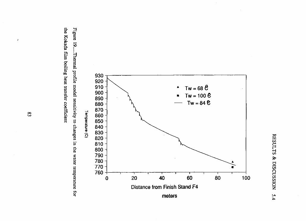

O
§
i Distance from Finish Stand F4 2: c ? meters ?

RESULTS & DISCUSSION
o o
o o o o o o o o m o m o w o m o O J C D c o o o r ^ r ^ c o c o
Temperature (C)
Figure 21 Thermal profile model literature heat transfer coefficients 0.05% carbon,
3.89 mm gauge, target coiling temperature 720*C.
85

RESULTS & DISCUSSION 5.4
o o
o o o o o o o o m o w o w o m o O > o > c o o 5 f » * r ^ c o c o
Temperature (C)
Figure 22 Thermal profile model literature heat transfer coefficients, 0.07% carbon,
0.024% Nb, 3.89 mm gauge, target coiling temperature 720°C.
86
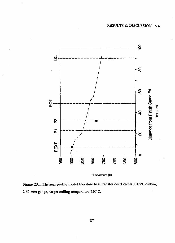
RESULTS & DISCUSSION 5.4
o o
c n o ) c o o o r ^ r > . c o c D
Temperature (C)
Figure 23 Thermal profile model literature heat transfer coefficients, 0.05% carbon,
2.62 mm gauge, target coiling temperature 720'C.
87

RESULTS & DISCUSSION 5.4
o o
o o o o o o o o m o m o m o u D O c o c n c o c o r « » r ^ c o c o
Temperature (C)
Figure 24 Thermal profile model literature heat transfer coefficients, 0.07% carbon,
0.024% Nb, 2.62 mm gauge, target coiling temperature 720 *C.
88

RESULTS & DISCUSSION 5.4
o o
o o o o o o o o i n o w o m o m o C O O J O O C O h - r ^ C O C O
Temperature (C)
Figure 25 Thermal profile model literature heat transfer coefficients, 0.05% carbon,
3.89 mm gauge, target coiling temperature 630*C.
89

RESULTS & DISCUSSION 5.4
Temperature (C)
Figure 26 A sample temperature profile from the plant data.
90
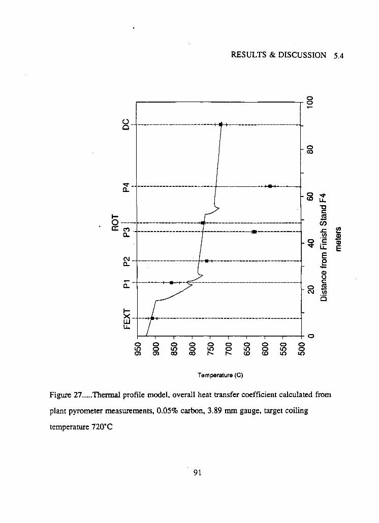
RESULTS & DISCUSSION
Temperature (C)
Figure 27 Thermal profile model, overall heat transfer coefficient calculated from
plant pyrometer measurements, 0.05% carbon, 3.89 mm gauge, target coiling
temperature 720"C
91

RESULTS & DISCUSSION
Temperature (C)
Figure 28 Thermal profile model, overall heat transfer coefficient calculated from
plant pyrometer measurements, 0.07% carbon, 0.024% Nb, 3.89 mm gauge, target
coiling temperature 720*C
92

RESULTS & DISCUSSION
o o
o o o o o o o o o o m o m o m o m o w o
Temperature (C)
Figure 29 Thermal profile model, overall heat transfer coefficient calculated from
plant pyrometer measurements, 0.07% carbon, 0.024% Nb, 2.62 mm gauge, target
coiling temperature 720'C
93

RESULTS & DISCUSSION
o o
o o o o o o o o o o i n o m o m o L o o m o o i c o o o o o r ^ r x - c o c o m i o
Temperature (C)
Figure 30 Thermal profile model, overall heat transfer coefficient calculated from
plant pyrometer measurements, 0.05% carbon, 2.62 mm gauge, target coiling
temperature 720°C
94
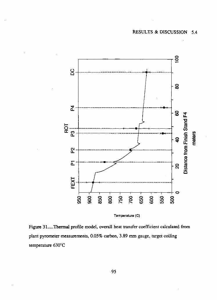
RESULTS & DISCUSSION
o o
o o o o o o o o o o L n o m o m o m o L o o c o c o o o o o r ^ r - c o c o m m
Temperature (C)
Figure 31 Thermal profile model, overall heat transfer coefficient calculated from
plant pyrometer measurements, 0.05% carbon, 3.89 mm gauge, target coiling
temperature 630* C
95

RESULTS & DISCUSSION
o o
o o o o o o o o o o L o o m o m o m o m o c 7 ) c o a o a o r « r ^ c o c o m m
Temperature (C)
Figure 32 Thermal profile model, overall heat transfer coefficient calculated from
plant pyrometer measurements, 0.05% carbon, 3.89 mm gauge, target coiling
temperature 550°C
96

RESULTS & DISCUSSION 5.4
o o
o o o o o o o o o o o o o fflcooiooooooooeoSsSNN
Temperature (C)
Figure 33 Thermal profile model sensitivity, Overall Heat Transfer Coefficient
Calculated from plant pyrometer measurements, 0.05% carbon, 3.89 mm gauge, target
coiling temperature 720° C
97

RESULTS & DISCUSSION
o o o o o o o o o o o o o o o o o o o o o o eo CM o cn oo h- co m ^ co CM t- o o> oo r*. co i n - r co cvj cjiO)0>oioococooocooococococor*»S-r^r»-r*»-S'r^r ,>.
Temperature (C)
Figure 34 Thermal profile model results for a 0.05 carbon, 3.89 mm gauge steel
using an individual laminar water bar heat transfer coefficient of 10 kW/m 2 °C and
showing the effect of using 20 kW/m2*C and 5 kW/m 2 o C on the target coiling
temperature of 720*C.
98

RESULTS & DISCUSSION 5.4
Fraction Transformed
Figure 35 Isothermal dilatometer results for 673*C test
99
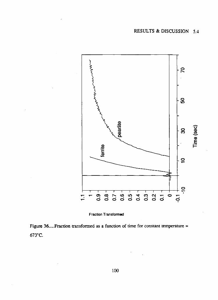
RESULTS & DISCUSSION 5.4
Fraction Transformed
Figure 36 Fraction transformed as a function of time for constant temperature =
673#C.
100

RESULTS & DISCUSSION
• \ • \
• \
CO CD
\ if) CO \ C\J
> CD «—«
Q
CO
CO II • \
r -
• \
OJ
h CNJ
CO
CM
CO ©
T T
d
d CVJ d in d
T - IT) CM i If)
c\i
In(ln(1/(1-Fx)))
Figure 37 Isothermal 673*C austenite to ferrite kinetics plotted as lnln(l/(l-FX))
versus ln(t).
101

RESULTS & DISCUSSION 5.4
ln(b), ferrite
Figure 38 ln(b) Avrami coefficient for the isothermal formation of ferrite in the 0.34
carbon steel.
102
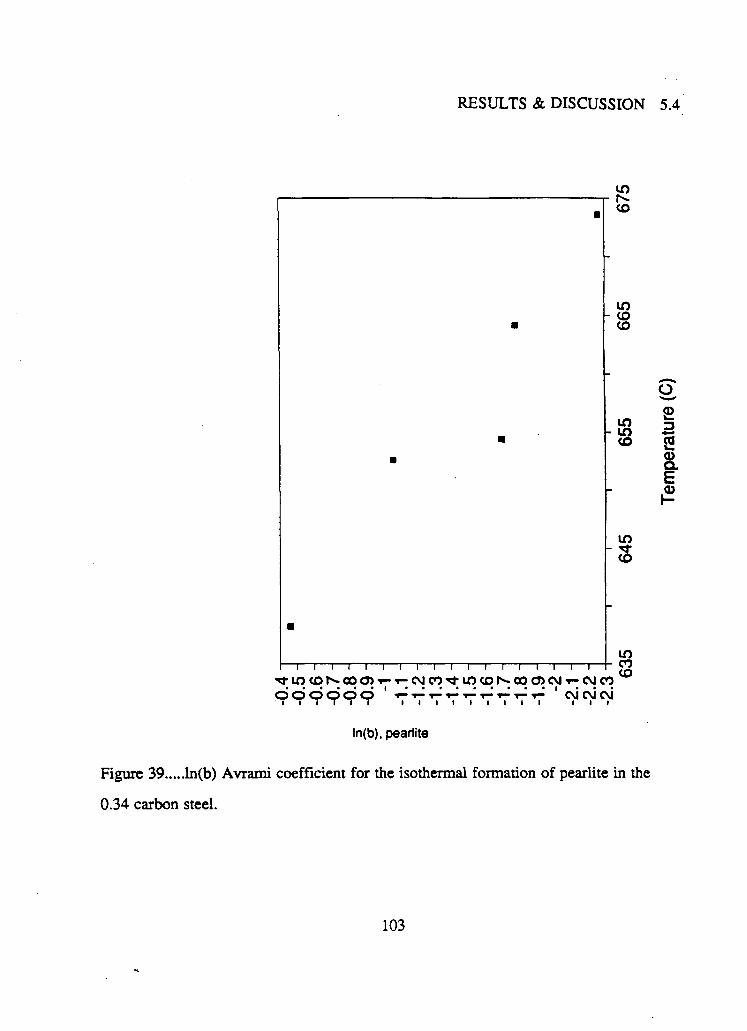
RESULTS & DISCUSSION
i i i i i i I i i i i i i i i i i r Tru3cor^coc»i-^CMcoTrir)cDr^coo>c\i-i-CMoo o o o o o o
i i i i i i I I I I I CM CM CM i i i
ln(b), pearlite
Figure 39 ln(b) Avrami coefficient for the isothermal formation of pearlite in the
0.34 carbon steel.
103

RESULTS & DISCUSSION 5.4
n (ferrite)
Figure 40 Avrami coefficient, n f, for the austenite-to-ferrite transformation in the 0.34
% C, plain carbon steel.
104

RESULTS & DISCUSSION
o
-O i _ C3 O o> CO
' c i I I i r
m co m CM m T -
C O ^ C M ^ to T -
o cn cn in oo
d
n (pearlite)
Figure 41 Avrami coefficient, n,,, for the austenite-to-pearlite transformation in the
0.34 % C, plain carbon steel.
105

RESULTS & DISCUSSION 5.4
ln(b), ferrite
Figure 42 Calculated ln(b) values for the ferrite transformation assuming ii f = 1.25,
for the 0.34% carbon steel.
106

RESULTS & DISCUSSION 5.4
ln(b), pearlite
Figure 43 Calculated ln(b) values for the pearlite transformation assuming ftp = 1.14,
for the 0.34% carbon steel.
107

RESULTS & DISCUSSION 5.4
LOTTOOCNJT—cxjo^cqr^couo CNJ C\i C\j C\i C\j T ^ T - ^ T - ^ T — i - ^ T - ^ - r ^ T - ^ - r ^ o o o o o
n v a l u e
Figure 44 Average Avrami coefficient V for 0.34% carbon compared to other
experimental values (Campbell[27])
108

RESULTS & DISCUSSION 5.4
+•
<
• x
x
r . r-. r*. r CM J CM I CM I C\l ) C\J <
CD CD CD CD CD CD CD CD CD CD To GO "55 CO GO Q
rr co CM T - 3 o o o o o n . T- y- -r- T - O
• + O < X «
o
o • +
+ +
CO
~ I I 1 I I
CM i - O i - CM CO r f i If)
O 00
o CO
o T t
o CM
o o
o oo
o CO
o rr
CM
CO
< h-o
s o CD
" O c 3
CO
ln(b), ferrite
Figure 45 Comparison of the ln(b) Avrami coefficient for the austenite-ferrite
transformation is several plain-carbon steels(Campbell[27]).
109

RESULTS & DISCUSSION 5.4
• 9 © <
O
co d
CD CD © CD CD CD CD CD CD CD CD CD
wcyScyjcy) c/5co com coo o o T -CMCOTT cor*, o o o o o o X < o + • >
CM,
"55 .O Q. E CO
O
o oo
o CO
_ o
o CM
CM T - O T - CM CO i i co 00
ln(b), pearlite
Figure 46 Comparison of the ln(b) Avrami coefficient for the austenite-ferrite
transformation is several plain-carbon steels(Campbell[27]).
110

RESULTS & DISCUSSION 5.4
Dilation - Temperature Figure 47 Dilatometer-time and temperature-time data for a continuous cooling rate
of 27'C/s*
111

RESULTS & DISCUSSION 5.4
112

RESULTS & DISCUSSION 5.4
Undercooling ( C ) (785 - Tst) Figure 49 The undercooling for the austenite-to-ferrite start temperature as a function
of the cooling rate.
113

RESULTS & DISCUSSION 5.4
I 1 1 1 1 1 1 i h o C O r ^ C O U O T T C O C N J - r - O o o o o o o o o
Percentage Ferrite
Figure 50....Fraction ferrite as a function of cooling rate, from metallographic
examination.
114

RESULTS & DISCUSSION
Figure 51 Continuously cooled dilatometer sample.
115

RESULTS & DISCUSSION
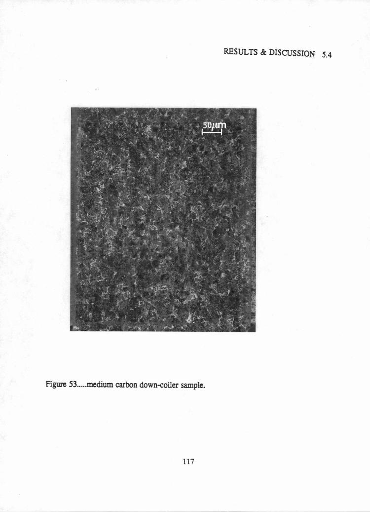
RESULTS & DISCUSSION

RESULTS & DISCUSSION
Temperature (C)
Figure 54 Surface thermal profile, using the overall heat transfer coefficient = 1
kW/m 2*C, Table DT-Run #1 cooling conditions, 3.94mm gauge, and a transformation
start temperature of 732'C ( dT/dt = 7'C/s).
118

RESULTS & DISCUSSION
o o
o o o o o o o o o o o o o o o o o C O r r c \ J O C O C D r f C \ J O O O C D T t C \ J O C O C O T t CnO5O)O)COCOCO00 0 0 S N N N N ( D t O ( O
Temperature (C)
Figure 55 Surface thermal profile, using the overall heat transfer coefficient = 1
kW/m 2*C, Table DJ-Run #2 cooling conditions, 3.94mm gauge, and a transformation
start temperature of 732'C ( dT/dt = 7'C/s).
119

RESULTS & DISCUSSION
o o
o o o o o o o o o o o o o o o o o C D ^ C N J O C O C D T f C N J O C O t O T r C N J O C O C O T f O l C I C n c n c O C O O O C O C O N N N N N O l D C D
Temperature (C)
Figure 5 6 Surface thermal profile, using the overall heat transfer coefficient = 1
kW/m 2*C, Table DI-Run #3 cooling conditions, 3.94mm gauge, and a transformation
start temperature of 732'C ( dt/dt = 7'C/s).
120

RESULTS & DISCUSSION
o o
O O O O Q O O O O O O O O O
O J O ) 0 > 0 0 0 0 0 0 0 0 0 3 N N N S N ( 0
Temperature (C)
Figure 57 Surface thermal profile, using the overall heat transfer coefficient = 1
kW/m 2*C, Table HI-Run #1 cooling conditions, 3.94mm gauge, and a transformation
start temperature of 688°C ( dt/dt = 45*C/s).
121

RESULTS & DISCUSSION
o o
o o o o o o o o o o o o o o t ( v J O 0 0 « 0 t C v | O 0 0 ( f i t C M O 0 0 O ) O ) O ) C O C O C O 0 0 0 0 N N N N N C O
Temperature (C)
Figure 58 Surface thermal profile, using the overall heat transfer coefficient = 1
kW/m 2 °C, Table Hi-Run #2 cooling conditions, 3.94mm gauge, and a transformation
start temperature of 688°C ( dt/dt = 45'C/s).
122

meters

RESULTS & DISCUSSION
o o
o o o o o o o o o o o o o o o o o c o r f o j o a j c D T r c N i o c o c o T r c M O c o c o r r cooJOTOioocooococo i^r^ .r^r^r^cococD
Temperature (C)
Figure 60 Surface thermal profile, using the literature heat transfer coefficients ,
Table DI-Run #1 cooling conditions, 3.94mm gauge, and a transformation start
temperature of 710*C ( dt/dt = 26*C/s).
124

RESULTS & DISCUSSION
Temperature (C)
Figure 61 Surface thermal profile, using the literature heat transfer coefficients ,
Table LTI-Run #2 cooling conditions, 3.94mm gauge, and a transformation start
temperature of 710"C ( dt/dt = 26'C/s).
125

RESULTS & DISCUSSION
Temperature (C)
Figure 62 Surface thermal profile, using the literature heat transfer coefficients ,
Table HI-Run #3 cooling conditions, 3.94mm gauge, and a transformation start
temperature of 710°C ( dt/dt = 26'C/s).
126

RESULTS & DISCUSSION 5.4
to in in in m U D m m m <<* -<t -t TJ- T T C O C O C O
Temperature (C)
Figure 63 Effect on predicted center line temperature of changes in the number of
nodes through thickness.
127

RESULTS & DISCUSSION 5.4
E E
co N
CO Q . ©
CO
Temperature (C)
Figure 64 Effect on predicted center line temperature of changes in the step size,
where the step size equals the strip velocity times the time increment.
128

RESULTS & DISCUSSION 5.4
o o
o o o o o o o o o o o o o o o T T C N O C O C O r f C N J O C O C O T f C N O C O C O C D O C n o O O O C O C O C O N N N N S C O C O
Temperature (C)
Figure 65 Effect of the ±0.3 m/s deviation of the strip velocity on the predicted
temperature profile.
129

RESULTS & DISCUSSION 5.4
Temperature (C)
Figure 66....Industrial cooling profile simulated on the Gleeble high temperature testing
machine.
130

RESULTS & DISCUSSION
Temperature (C)
Figure 67 Industrial cooling conditions, simulated on a Gleeble high temperature
testing machine.
131

RESULTS & DISCUSSION 5.4
Figure 68 Microstructure of the Gleeble cooling simulation sample of the Table UJ
run one cooling conditions.
132

CONCLUSIONS 6.1
6 CONCLUSIONS
6.1 Summary
A mathematical model has been formulated to predict the through thickness
temperature distribution of strip as it cools on the run-out table of a hot-strip mill. The
model incorporates the heat of transformation associated with the austenite to ferrite
and ferrite plus pearlite phase change.
The phase transformation has been characterized by an Avrami equation and the
coefficients, n and b, have been determined from isothermal diametral dilatometer tests.
The transformation start temperature is a function of the cooling rate experienced by
the steel and a relationship between the cooling rate and the temperature at which the
phase transformation starts has been determined from continuous cooling diametral
dilatometer tests.
The total fraction ferrite that will form is also a function of the cooling rate and
the fraction ferrite has been characterized as a function of cooling rate using the
quantitative analysis capability of the Wild-Leitz image analyzer with polished and
etched continuous cooling test samples.
In-plant temperature measurements for various strip cooling regimes were
obtained and used with the thermal profile model to calculate an overall effective heat
transfer coefficient for a laminar water bar cooling bank. Back calculation of a heat
transfer coefficient for individual laminar water bar headers using the plant temperature
data was unsuccessful due to the insensitivity of the strip temperature to individual
133
CONCLUSIONS 6.1
laminar water bars due to the short strip residence rime under any individual header.
Metallographic examination of strip samples from the in-plant temperature data
acquisition tests to determine a relationship between coiling temperature and grain size
was inconclusive as no obvious relationship was seen.
Heat transfer coefficients for various cooling regimes; laminar water bar, water
curtain, film boiling, support roll contact, and air cooling by convection/radiation, were
found in the literature. These values were used in the overall model incorporating
phase transformation along with industrial cooling conditions to predict strip thermal
profiles and the predicted temperatures were compared with plant pyrometer values.
The effect of variations in the various heat transfer coefficients on the model
thermal profile predictions was examined and the model was shown to be relatively
insensitive to small variations in the heat transfer coefficients obtained from literature
or calculated. The model did, however, show some sensitivity to variations in strip
velocity.
The cooling regime predicted by the overall model, incorporating phase
transformation, was simulated on a Gleeble 1500 testing machine. The resulting
transformation start temperature of 730*C is similar to that predicted by the emperical
transformation start versus constant cooling rate data for an average cooling rate of
7'C/s.
The dilatometer test samples were from transfer bar stock, due to specimen size
constraints, and had not received the finish stand rolling that a down_coiled sample
would. To determine the validity of using transfer bar stock to predict down-coiled
134
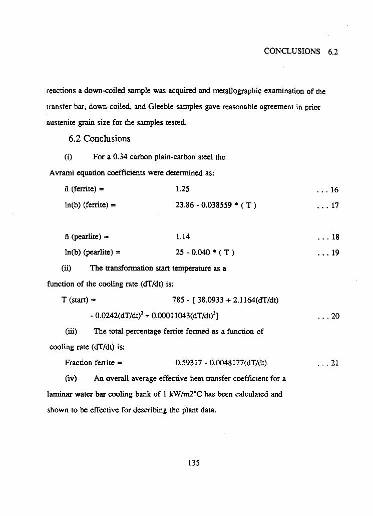
CONCLUSIONS 6.2
reactions a down-coiled sample was acquired and metallographic examination of the
transfer bar, down-coiled, and Gleeble samples gave reasonable agreement in prior
austenite grain size for the samples tested.
6.2 Conclusions
(i) For a 0.34 carbon plain-carbon steel the
Avrami equation coefficients were determined as:
n (ferrite) = 1.25 . . . 16
ln(b) (ferrite) = 23.86 - 0.038559 * ( T ) . . . 17
fi (pearlite) = 1.14 . . . 18
ln(b) (pearlite) = 25 - 0.040 * ( T ) . . . 19
(ii) The transformation start temperature as a
function of the cooling rate (dT/dt) is:
T (start) = 785 - [ 38.0933 + 2.1164(dT/dt)
- 0.0242(dT/dt)2 + 0.00011043(dT/dt)3] . . . 20
(iii) The total percentage ferrite formed as a function of
cooling rate (dT/dt) is:
Fraction ferrite = 0.59317 - 0.0048177(dT/dt) . . . 21
(iv) An overall average effective heat transfer coefficient for a
laminar water bar cooling bank of 1 kW/m2'C has been calculated and
shown to be effective for describing the plant data.
135

CONCLUSIONS 6.2
(v) An individual laminar water bar heat transfer coefficient
cannot be calculated with the present data due to the short residence time of
the strip under any one individual spray.
(vi) While no correlation between grain size and coiling
temperature was observed, a larger number of tests might separate trends
from experimental scatter.
(vii) The overall model, incorporating phase transformation,
calculated a strip thermal profile for various industrial cooling conditions, for
a 0.34 carbon plain-carbon steel. For the calculated overall heat transfer
coefficient of 1 kW/m 2 , C, using a transformation start temperature of 732"C
calculated for the cooling rate of 7*C/s experienced in the air cooling section
of the run-out table, the model predicted temperatures 19*C to 24*C greater
than the measured pyrometer values.
(viii) For the same conditions as in (vii) with a transformation start
temperature of 688'C calculated for the 45*C/s cooling rate experienced in
the water cooling section of the run-out table, the model predicted
temperatures of l ' C to 5*C greater than the pyrometer readings.
(ix) Using the literature derived heat transfer coefficient values
instead of the calculated overall heat transfer coefficient, with the same
cooling conditions as in (vii) and (viii), and a cooling rate of 26°C/s, which
is the average of the 45*C/s and 7*C/s values, model predictions were
compared with pyrometer values. For this cooling rate the transformation
136
CONCLUSIONS 6.2
start temperature is 710*C and the model predictions are 25*C to 33'C
greater than the plant pyrometer readings. These literature derived heat
transfer coefficients are useful but require fine tuning for the effects of strip
velocity which was not present in the initial experiments used to produce
these relationships.
(x) The cooling regime used for the model predictions was
simulated on a Gleeble testing machine and the model predictions were
within XX* C of the simulation temperatures. The simulation sample started
phase transformation at approximately 730" C which is also the
experimentally produced transformation start temperature for a cooling rate
of 7'C/s.
(xi) The continuous cooling and Gleeble test samples, made from
transfer bar stock, and a down-coiler sample, where examined to compare
the prior austenite grain sizes. The average prior austenite grain size for the
continuous cooling dilatometer samples of 29 um ± 8 um compares well
with the down-coiler value of 35 um ± 9 um. The Gleeble sample shows
some local microstructural variation due to banding, as shown in Figure 68,
and an average austenite grain size of 18 um ± 3 urn. This grain size is
finer than that obtained in the continuous cooling transformation samples but
is similar in magnitude. The closer austenite grain size similarity between
the continous cooling samples and the down-coiler sample supports the use
of transfer bar to measure the transformation kinetics.
137

CONCLUSIONS 6.3
6.3 Future Considerations
Modification of the existing hardware to allow characterization of other low
carbon and HSLA grades of steel as well as duplication of the prior thermo-mechanical
history is needed to increase the scope of the work. The addition of the Gleeble high
temperature testing machine means that the deformation due to the finishing stands may
be duplicated in the future or that a method of using test samples of smaller dimensions
will allow the use of down-coiler samples rather than the transfer bar samples currently
employed. Modifications to the model to include prior thermo-mechanical history and
grain growth effects prior to the run-out table should be added to allow grain growth
prediction on the run-out table as well as prediction of final grain size and thus some
mechanical properties prediction. As the grades of steel that can be characterized are
increased the bainite and martensite phase transformation kinetics should be
characterized to increase the scope of the model.
Finally the run-out table model could be integrated into an overall rolling mill
model for use in production forecasting.
138

BIBLIOGRAPHY 7
7 BIBLIOGRAPHY
1 G. Tacke, H. Litzke and E . Raquet, "Investigations into the Efficiency of cooling systems for Wide-Strip Hot Rolling Mills and Computer-aided Control of Strip Cooling", Accelerated Cooling of Steel, Proceedings of a symposium sponsored by The Metallurgical Society of AIME, Pittsburgh, Pennsylvania, August 19-21, 1985, pp 35-54.
2 R. Colas and C M . Sellars, "Computed Temperature Profiles of Hot Rolled Plate and Strip During Accelerated Cooling", (CTM convention , Winnipeg, Manitoba 1987)
3 E.A. Farber and R.L. Scorah, "Heat Transfer to Water Boiling Under Pressure", Transactions of the A S M E , 70 (1948), pp.369-384.
4 Natsuo Hatta, Jun-ichi Kokada and Koichi Hanasaki, "Numerical Analysis of Cooling Characteristics for Water Bar", Transactions of ISU, Volume 23, 1983, pp 555-564.
5 Natsuo Hatta, Jun-ichi Kokada, Hirohiko Takuda, Jun Harada and Keizo Hiraku, "Predictable Modeling for Cooling Process of a Hot Steel Plate by Laminar Water Bar", Archiv fur das Eisenhuttenwesen, 55(1984) Nr. 4 April, pp.143-148.
6 Jun-ichi Kokada, Natsuo Hatta, Hirohiko Takuda, Jun Harada and Nobuo Yasuhira, "An Analysis of Film Boiling Phenomena of Subcooled Water Spreading Radially on a Hot Steel Plate", Archiv fur das Eisenhiittenwessen, Nr. 55(1984) March
7 Arnulf Diener and Alfons Drastik, "Heat Exchange Between Strands and Guide Rollers in the Secondary Cooling Zone of a Slab Continuous Casting Machine", Fourth Japan-Germany Seminar, Nov. 1980, Tokyo, The Iron And Steel Institute of Japan
8 "Physical Constants of Some Commercial Steels at Elevated Temperatures", Edited by the British Iron and Steel Research Association, Metallurgy (General) Division Thermal Treatment Sub-Committee, London, 1953
9 M . A^rami: "Kinetics of Phase Change. I, General Theory", Journal of Chemical Physics, December 1939, pp.1103-12.
10 M . Avrami: "Kinetics of Phase Change. LI, Transformation-Time Relations for Random Distribution of Nuclei", Journal of Chemical Physics, February 1940, pp.212-224.
139

BIBLIOGRAPHY 7
11 M. Avrami: "Granulation, Phase Change, and Microstructure. Kinetics of Phase Change HI", Journal of Chemical Physics, February 1941, pp. 177-84.
12 J.W. Cahn, "The Kinetics of Grain Boundary Nucleated Reactions", Acta Metallurgies Vol. 4, September 1956, pp.449-459.
13 Prakash K. Agarwal and J.K. Brimacombe, "Mathematical Model of Heat Flow and Austerute-Pearhte Transformation in Eutectoid carbon Steel Rods for Wire", Metallurgical Transactions B, Vol 12B, March 1981, pp.121-133.
14 M.B. Kuban, R. Jayaraman, E.B. Hawbolt, and J.K. Brimacombe: "An Assessment of the Additivity Principle in Predicting Continuous-Cooling Austenite-to-Pearlite Transformation Kinetics Using Isothermal Transformation Data", Metallurgical Transactions A, Vol. 17A, September 1986, pp. 1493-1503.
15 E.B. Hawbolt, B. Chau, and J.K. Brimacombe, "Kinetics of Austenite-Pearlite Transformation in Eutectiod Carbon Steel", Metallurgical Transactions A, Vol. 14A, September 1983, pp.1803-15.
16 E.B. Hawbolt, B. Chau, and J.K. Brimacombe: "Kinetics of Austenite-Ferrite and Austenite-Pearlite Transformations in a 1025 Carbon Steel", Metallurgical Transactions A, Vol. 16A, April 1985, pp.565-77.
17 M . Morita, K. Hashiguchi, O. Hashimoto, M . Nishida, and S. Okano, "On-Line Transformation Detector for Property Control of Hot Rolled Steel", Accelerated Cooling of Steel, Proceedings of a symposium sponsored by The Metallurgical Society of AJME, Pittsburgh, Pennsylvania, August 19-21, 1985, pp.449-461
18 Eric N. Hinrichsen, "Hot Strip Mill Runout Table Cooling - A System View of Control, Operation and Equipment", Yearly Proceedings of the AISE, 1976, pp.403-408.
19 A. Hurkmans, G.A. Duit, Th.M. Hoogendoom and F. Hollander, "Accelerated cooling and the Transformation of Steel", Accelerated Cooling of Steel, Proceedings of a symposium sponsored by The Metallurgical Society of AIME, Pittsburgh, Pennsylvania, August 19-21, 1985, pp.481-499
20 Edward B. Longenberger, "Computer Modeling of a Hot Strip Mill Run out Table", Proceedings of the XXVIII Conference on Mechanical Working and Steel Processing, The Iron and Steel Society of the AIME, Pittsburgh, PA, October 26-28, 1986, pp. 169-172
140

BIBLIOGRAPHY 7
21 Yushi Miyake, Teruyuki Nishide and Shoichi Moriya, "Device and System for Controlled Cooling for Hot Strip Mill", Transactions of the ISIJ, vol 20, 1980 pp.496-503
22 H. Yada, "Prediction of Microstructural Changes and Mechanical Properties in Hot Strip Rolling", Presented at the Accelerated Cooling of Steel Symposium at the Conference of the Canadian Institute of Mining and Metallurgy, Winnipeg, Manitoba, August 24, 1987.
23 Zacay and AAronson editors, "Decomposition of Austenite by Diffusional Processes", 1962, pp. 336
24 P J . Berensen, "Film-Boiling Heat Transfer From a Horizontal Surface", Transactions of the A S M E , Journal of Heat Transfer, vol 83, August 1961, pp.351-358.
25 K.W. Andrews, "Empirical Formula for the Calculation of Some Transformation Temperatures", Journal of the Iron and Steel Institute, July 1965, pp. 721-727
26 A. le Bon, J. Rofes-Vemis, and C. Rossard, "Recrystallization and Precipitation during Hot Working of a Nb-Bearing HSLA Steel", Metal Science, volume 9, 1975, pp36-40.
27 P. Campbell, Private communication of unpublished work.
28 C. Devadas, Private communication of unpublished work.
29 Yukihisa Kuriyama, Matsuo Ataka, Masayuki Nakanishi, Masayuki Miyatake, Kouichiro Goto and Shuichi Hamauzu, "On-line Model for Prediction of Strip Temperature in Hot Rolling", Transactions of the ISIJ, vol. 23 number 9, 1983, p.B338.
30 J.S. Kirkaldy and E.A. Baganis, "Thermodynamic Prediction of the Ae3 Temperature of Steels with Additions of Mn, Si, Ni, Cr, Mo, Cu", Metallurgical Transactions A, Vol. 9A, April 1978, pp.495-501.
141

APPENDIX
APPENDIX
8.1 N O M E N C L A T U R E
*/ Avrami coefficient, 'b' for ferrite
K Avrami coefficient, 'b' for pearlite
c. Specific heat, (W/kg*C)
D Laminar water bar nozzle internal diameter, (m)
Fx(k -1) Fraction transformed in the previous time step
Fx(k) Fraction transformed in the current time step
8 Acceleration due to gravity, (m/s2)
h Heat transfer coefficient, (W/m2*C)
H Laminar water bar header height over run-out table, (m)
k Thermal conductivity, (W/m'C)
nf Avrami coefficient, V for ferrite
NP Avrami coefficient, V for pearlite
"/ average n(ferrite)
"P average n(pearlite)
Pr Prandtl number
4. Heat flux generated due to phase transformation, (W)
Q Water flow rate, (m3/s)
r Laminar water bar contact radius, (m)
Re Reynolds number
142

APPENDIX 8.1
t Time, (s)
tv Virtual time, (s)
/• Time for completion of 20% of the phase
transformation, (s)
r Time for completion of 90% of the phase
transformation, (s)
TCRTT Critical water temperature for film boiling
to water contact cooling transition, (*C)
T(k) Node temperature at this time step, (°C)
7(j y Internally calculated model temperature values, (*C)
T(k) Internally calcualted model temperature values, (*C)
Ts Steel surface temperature, (°C)
TSAJ. Water saturation temperature, (*C)
T Transformation start temperature, (*C)
Tw Water temperature, (*C)
x,y,z Spatial coordinates, (m)
X Fraction transformed
a Ferrite phases
a n Film boiling heat transfer coefficient, (W/m 2 ,C)
ot j Laminar water bar heat transfer coefficient, (W/m 2 #C)
y Austenite phase
5 Water film thickness, (m)
143

APPENDIX 8.1
6V Thermally affected water film thickness, (m)
AFx{k),dFx(k) Incremental fraction transformed for this time step
At,dt Model time step, (s)
Ax,etc Model step size, (m)
Az Model node size, (m)
e Emissivity
v Strip velocity, (m/s)
p Density, (kg/m3)
ej Stefan Boltzmann constant, (W/m 2K 4)
144
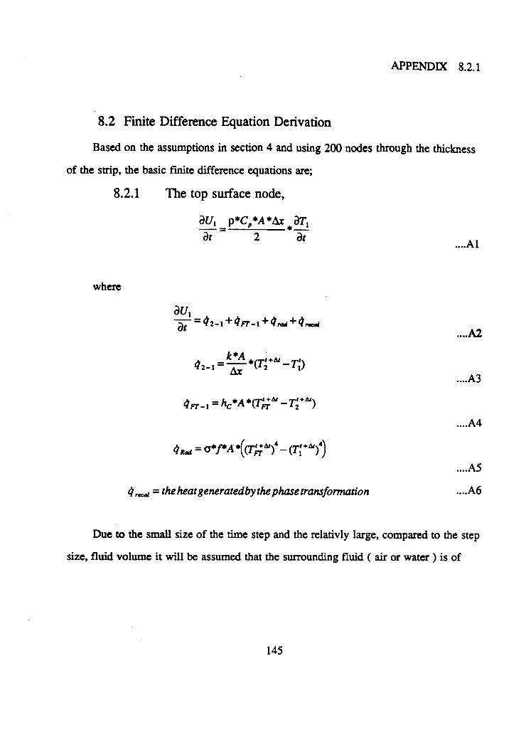
APPENDIX 8.2.1
8.2 Finite Difference Equation Derivation
Based on the assumptions in section 4 and using 200 nodes through the thickness
of the strip, the basic finite difference equations are;
8.2.1 The top surface node,
dUt p*C*A*bc^dTx
dt ~ 2 * dt
where
dUi -jfi- = <?2-1 + 4lT- 1 + Qrad + 4
4Fr-l=hc*A*<T'Fr"-T2'+")
.Al
....A2
....A3
....A4
....AS
Qnai = the heat generatedby the phase transformation ....A6
Due to the small size of the time step and the relativly large, compared to the step
size, fluid volume it will be assumed that the surrounding fluid ( air or water) is of
145

APPENDIX 8.2.2
constant temperature. To facilitate the solution of the radiation calculations the node
temperature from the current time step is used for the future time step calculations.
Which results in the equation :
2A/ 1 1 2
.A7
f p * C , * A ^ 1 2A/
8.2.2 Interior nodes
The interior nodes were less difficult to describe due to the absence of radiation
or convection effects in Eq.A.7. Through a similar set of assumptions to those in the
top surface node, Eq.A.8 was produced.
o*C *Ar
^ ....A8
= T'* * a
+4 rtcai 2*Ar
8.2.3 The bottom node
As with the formulation of the top surface node (1) equations and with similar
fluid temperature and radiation cooling simplifications the bottom node, node 'n' in this
example, could be described, after manipulation by Eq.A.9.
146

APPENDIX 8.3
-k*Ax*T. • -I ....A9
„JP*C,*Ax + hc*T'„ + a*f^(T'J-(T:)) + <i rtcai
8.2.4 Solution
The equations for the top and bottom surfacve nodes along with the
interior nodes can be gatherd together as a sparse tridiagonal matrix. A
number of simple subroutines exist to make this problem readily solvable by
computer.
8.3 Hatta et al. Model Thermal Boundary Layer Calculation
The thermal boundary layer concept used by Hatta et al. is effected by the water
velocity, which is calculated with
where Q is the water flow rate in m 3 / min, D is the diameter of the laminar water bar
nozzle in meters, H is the height above the strip in meters, and g is the acceleration due
to gravity. The thickness of the water film layer is then calculated by Eq.A. l 1.
....A10
. . .All k*dr 2KVW
147
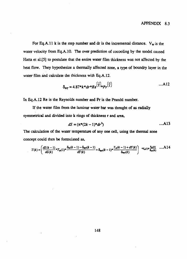
APPENDIX 8.3
For Eq.A. l 1 k is the step number and dr is the incremental distance. V w is the
water velocity from Eq.A.10. The over prediction of cocooling by the model caused
Hatta et al.[5] to postulate that the entire water film thickness was not affected by the
heat flow. They hypothesize a thermally affected zone, a type of boundry layer in the
water film and calculate the thickness with Eq.A.12.
In Eq.A.l2 Re is the Reynolds number and Pr is the Prandd number.
If the water film from the laminar water bar was thought of as radially
symmetrical and divided into k rings of thickness r and area,
The calculation of the water temperature of any one cell, using the thermal zone
concept could then be formulated as,
....A12
dS = (7C*(2* - l)*dr2) ....A13
T(k) = rdS(k-l) , dS(k)
oy*-l)-cW*-l) dTik)
+ 8wr(*-l)' M i ....A14
148


![Modified Jominy Test for Determining the Critical Cooling Rate for Intercritically Annealed Dual Phase Steels [2]](https://img.pdfslide.us/doc/110x75/557207a1497959fc0b8bb33c/modified-jominy-test-for-determining-the-critical-cooling-rate-for-intercritically-annealed-dual-phase-steels-2.jpg)