Embed Size (px)
Citation preview
Southern Methodist University Southern Methodist University
SMU Scholar SMU Scholar
Earth Sciences Theses and Dissertations Earth Sciences
Spring 5-15-2021
Characterization of Landslide Processes From Radar Remote Characterization of Landslide Processes From Radar Remote
Sensing and Hydromechanical Modeling Sensing and Hydromechanical Modeling
Yuankun Xu [email protected]
Follow this and additional works at: https://scholar.smu.edu/hum_sci_earthsciences_etds
Part of the Environmental Monitoring Commons, Fluid Dynamics Commons, Geological Engineering
Commons, Geology Commons, Geomorphology Commons, Geophysics and Seismology Commons,
Geotechnical Engineering Commons, Hydrology Commons, Mechanics of Materials Commons, Other
Earth Sciences Commons, Soil Science Commons, and the Tectonics and Structure Commons
Recommended Citation Recommended Citation Xu, Yuankun, "Characterization of Landslide Processes From Radar Remote Sensing and Hydromechanical Modeling" (2021). Earth Sciences Theses and Dissertations. 19. https://scholar.smu.edu/hum_sci_earthsciences_etds/19
This Dissertation is brought to you for free and open access by the Earth Sciences at SMU Scholar. It has been accepted for inclusion in Earth Sciences Theses and Dissertations by an authorized administrator of SMU Scholar. For more information, please visit http://digitalrepository.smu.edu.
CHARACTERIZATION OF LANDSLIDE PROCESSES FROM RADAR REMOTE
SENSING AND HYDROMECHANICAL MODELING
Approved by:
_______________________________________ Prof. Zhong Lu Professor of Geophysics _______________________________________ Dr. David George Research Mathematician (USGS) _______________________________________ Dr. Jinwoo Kim Research Scientist of Geophysics _______________________________________ Prof. Robert Gregory Professor of Geochemistry _______________________________________ Prof. Matt Hornbach Associate Professor of Geophysics
CHARACTERIZATION OF LANDSLIDE PROCESSES FROM RADAR REMOTE SENSING
AND HYDROMECHANICAL MODELING
A Dissertation Presented to the Graduate Faculty of Dedman College
Southern Methodist University
in
Partial Fulfillment of the Requirements
for the degree of
Doctor of Philosophy
with a
Major in Geophysics
by
Yuankun Xu
B.S., Geospatial Engineering, China University of Mining and Technology, Xuzhou, China
May 15, 2021

Copyright (2021)
Yuankun Xu
All Rights Reserved
iv
Xu, Yuankun B.S., China University of Mining and Technology
Characterization of Landslide Processes from Radar Remote Sensing and Hydromechanical Modeling Advisor: Professor Zhong Lu
Doctor of Philosophy conferred May 15, 2021
Dissertation completed April 26, 2021
Landsides are a natural geomorphic process yet a dangerous hazard which annually causes
thousands of casualties and billions of property loss in a global scale. Understanding landslide
motion kinematics from early initiation to final deposition is critical for monitoring, assessing, and
forecasting landslide movement in order to mitigate their hazards. Landslides occur under diverse
environmental settings and appear in variable types; however, all types of landslides can be
mechanically attributed to shearing failure at the basal surface due to stress regime shift contributed
by internal and/or external forcing. Typical internal factors include soil/rock weathering, whereas
typical external triggering forces encompass precipitation, groundwater, tectonic activity,
landslide toe cutting, and landslide head loading. Physically, kinematics of most natural hillslope
failures from instigation to cessation can be approached as a hydromechanical problem.
Variable types of landslides were examined and characterized in this thesis from integrating
satellite/airborne remote sensing and hydromechanical modeling, with the intention to generate
insights for reducing landslide hazards globally. In particular, high-resolution satellite optical and
radar images and airborne lidar Digital Elevation Models (DEMs) were extensively utilized
through advanced quantitative techniques such as sub-pixel offset tracking and radar
interferometry in order to capture landslide motion dynamics. Modeling efforts were incorporated
to mechanically interpret the observed landslide kinematics and to further generate insights for
v
evaluating and forecasting other similar landslides. The five case studies detailed in this thesis
involve multiple distinct landslide behaviors and hydromechanical settings which are typical for
many worldwide. Particularly, these investigations entail a consistently slow seasonal landslide,
an alternately slow and rapid coastal landslide, a retrogressive and potentially catastrophic
headscarp landslide, multiple irrigation-triggered slow and catastrophic landslides, and hundreds
of other slow landslides near the U.S. west coast. Knowledge from hydrogeology, soil mechanics,
grain-flow mechanics, and fluid mechanics was integrated to decipher and model the impacts on
landslide dynamics from bedrock lithology, land uplift, precipitation-contributed pore pressure,
groundwater, soil shearing dilation and contraction, and basal topography. From these five
landslide case studies near the U.S. west coast, we were able to obtain enhanced understanding of
the landslide processes and numerically characterize the key elements from failure instigation to
movement evolution, interaction with waterbodies on the runout path, and final deposition.
Our investigations particularly demonstrated the potential of integrating satellite observations
and hydromechanical modeling to enhance our understanding of landslides and to reduce their
hazards. Insights generated from our case studies are applicable to many similar landslides
worldwide for their movement characterization and hazard assessment. Hence, this thesis was also
aimed to motivate similar efforts globally for landslide hazard mitigation, especially in response
to the projected increasingly frequent landslide events in the near future due to global climate
change and expanding anthropogenic activities.

vi
TABLE OF CONTENTS
LIST OF FIGURES ………………………………………………………………......…...….… xii
LIST OF TABLES …………………………………………………………………..…...…..…. xv
ACKNOWLEDGEMENTS ……………………………………………………...……………. xvi
CHAPTER 1: INTRODUCTION ................................................................................................... 1
1.1 Radar Remote Sensing .......................................................................................................... 2
1.1.1 SAR imaging .................................................................................................................. 2
1.1.2 InSAR ............................................................................................................................ 5
1.2 Landslide Processes .............................................................................................................. 8
1.3 Chapter Summarizes and Contributions ............................................................................. 10
References ................................................................................................................................. 16
CHAPTER 2: CHARACTERIZING SEASONAL MOTION OF THE SLOW-MOVING LAWSON CREEK LANDSLIDE, OREGON ..................................................... 20
2.1 Introduction ......................................................................................................................... 20
2.2 Landslide Location and Geological Settings ...................................................................... 22
2.3 Materials and Methods ........................................................................................................ 22
2.3.1 SAR Interferometry for Landslide Time-series Mapping ............................................ 22
2.3.2. Thickness Inversion .................................................................................................... 26
2.3.3 Time Lags .................................................................................................................... 28
2.3.4 Failure Depth using Limit Equilibrium Analysis ......................................................... 29
2.4 Results ................................................................................................................................. 32
vii
2.4.1 Time-series Displacements and Annual Deformation Rates ....................................... 32
2.4.2 Time Retardation to Seasonal Precipitation ................................................................. 34
2.4.2 Basal Depths and Volume Infered from InSAR Observations .................................... 39
2.4.3 Failure Depths from Limit Equilibrium Analysis ........................................................ 40
2.4.4 Potential for Estimating Hydraulic Parameters ............................................................ 42
2.5 Discussion ........................................................................................................................... 43
2.6 Conclusions ......................................................................................................................... 45
Acknowledgments ..................................................................................................................... 47
References ................................................................................................................................. 49
CHAPTER 3: DYNAMICS AND PHYSICS-BASED RAINFALL THRESHOLDS FOR THE DEEP-SEATED HOOSKANADEN LANDSLIDE, OREGON .......................... 54
3.1 Introduction ......................................................................................................................... 54
3.2 Geological Setting and Historical Activities ....................................................................... 57
3.2.1 Geographical and Geological Settings ......................................................................... 57
3.2.2 Historical Moderate and Major Slide Movements ....................................................... 60
3.3 Data and Methodology ........................................................................................................ 60
3.3.1 Data .............................................................................................................................. 60
3.3.2 InSAR .......................................................................................................................... 62
3.3.3 Pixel Offset Tracking ................................................................................................... 63
3.3.3.1 Preprocessing of Sentinel-1/2 images ................................................................... 64
3.3.3.2 Preprocessing of LiDAR DEMs ........................................................................... 65
3.3.4 Reconstruction of Three-dimensional Displacement Field .......................................... 66
viii
3.4 Results ................................................................................................................................. 67
3.4.1 Three-dimensional Displacement Field of the February 2019 Event .......................... 67
3.4.2 Movement Rate from Airborne LiDAR DEMs ........................................................... 69
3.4.3 Motion Dynamics from 2007 to 2019 .......................................................................... 71
3.4.4 Estimation of Hydraulic Conductivity and Diffusivity ................................................ 76
3.5 Discussion ........................................................................................................................... 78
3.5.1 Enhancement of Pixel Offset Tracking ........................................................................ 78
3.5.2 Proposed Rainfall Threshold for the Moderate/Major Events ..................................... 80
3.5.3 Mechanism of Landslide Motions Modulated by Precipitation and Coastal Erosion . 83
3.6 Conclusions ......................................................................................................................... 85
Acknowledgments ..................................................................................................................... 86
References ................................................................................................................................. 88
CHAPTER 4: MOVEMENT MONITORING AND RUNOUT HAZARD ASSESSMENT OF THE GOLD BASIN LANDSLIDE, WASHINGTON ......................................... 91
4.1 Introduction ......................................................................................................................... 91
4.2 Geological Setting and History ........................................................................................... 96
4.2.1 Regional Setting ........................................................................................................... 96
4.2.2 Historical Landslide Activity ....................................................................................... 96
4.3 Methodology and Data ........................................................................................................ 97
4.3.1 Measuring Landslide Movement Using Remote Sensing ............................................ 97
4.3.1.1 LiDAR DEM differencing .................................................................................... 97
4.3.1.2 InSAR ................................................................................................................... 98
4.3.1.3 SAR intensity differencing and pixel offset tracking ......................................... 100

ix
4.3.2 Runout Scenario Simulation ...................................................................................... 101
4.3.2.1 D-claw model ...................................................................................................... 101
4.3.2.2 Log-spiral basal surfaces ..................................................................................... 104
4.3.2.3 Landslide volume estimations ............................................................................. 106
4.3.2.4 D-claw simulations setup .................................................................................... 107
4.4 Results ............................................................................................................................... 108
4.4.1 Remote Sensing of Landslide Activity ...................................................................... 108
4.4.1.1 LiDAR DEM differencing .................................................................................. 108
4.4.1.2 InSAR ................................................................................................................. 108
4.4.1.3 SAR intensity changes and pixel offset tracking ................................................ 109
4.4.2 Simulations of Hypothetical Runout Scenarios ......................................................... 113
4.4.3 Simulations of Interactions with the Stillaguamish River ......................................... 116
4.5 Discussion ......................................................................................................................... 120
4.6 Conclusions ....................................................................................................................... 121
Acknowledgments ................................................................................................................... 122
References ............................................................................................................................... 124
CHAPTER 5: GEOLOGIC CONTROLS OF SLOW-MOVING LANDSLIDES HIDDEN NEAR THE U.S. WEST COAST ................................................................................... 127
5.1 Introduction ....................................................................................................................... 127
5.2 Materials and Methods ...................................................................................................... 129
5.2.1 SAR Interferogram Generation and Unwrapping ...................................................... 129
5.2.2 Identification of Active Landslides ............................................................................ 131
5.2.3 Bedrock of the Landslides ......................................................................................... 131
x
5.2.4 Landslide Area-volume Scaling and Average Slope Angle ...................................... 135
5.2.5 Land Uplift Rate ........................................................................................................ 135
5.3 Results ............................................................................................................................... 137
5.3.1 Discovery of Hidden Landslide Hazards ................................................................... 137
5.3.2 Bedrock Control of Slow-moving Landslides ........................................................... 141
5.3.3 Landsliding Contributed by Land Uplift .................................................................... 145
5.4 Discussion and Conclusions ............................................................................................. 147
5.4.1 Landslide Identification Using Radar Interferometry ................................................ 147
5.4.2 Geologic Impacts on Landslide Character and Kinematics ....................................... 149
5.4.3 Hydrological Impacts on Landslide Motion .............................................................. 149
5.4.4 Implication on Landslide and Geomorphic Studies ................................................... 152
Acknowledgments ................................................................................................................... 152
References ............................................................................................................................... 155
CHAPTER 6: KINEMATICS OF IRRIGATION-INDUCED LANDSLIDES IN A WASHINGTON DESERT: PRELIMINARY RESULTS.................................. 161
6.1 Introduction ....................................................................................................................... 161
6.2 Study Area ........................................................................................................................ 163
6.3 Data and Methods ............................................................................................................. 165
6.3.1 Data ............................................................................................................................ 166
6.3.2 Multitemporal InSAR Processing .............................................................................. 166
6.3.3 Forced Water Circulation on A Wavy Sliding Surface ............................................. 167
6.4 Preliminary Results ........................................................................................................... 171
xi
6.4.1 Mapping Slow and Catastrophic Landslides .............................................................. 171
6.4.2 Kinematics of Slow Landslides ................................................................................. 175
6.4.2.1 The slow life cycle from initiation to deposition ................................................ 175
6.4.2.2 Slow motion modulated by external force disturbances ..................................... 178
6.4.3 Kinematics of Catastrophic Landslides ..................................................................... 182
6.4.4 Landslide Motion Regulated by Basal Topography .................................................. 184
6.4.4.1 Basal topography regulates slow landslides by forced water circulation ........... 184
6.4.4.2 Basal topography bifurcates slow and catastrophic movements ......................... 186
6.5 Discussion ......................................................................................................................... 190
6.5.1 Satellite Imagery for Landslide Identification and Monitoring ................................. 190
6.5.2 Human-Induced Landslides and Potential Prevention Measures ............................... 191
6.5.3 Implications of Basal Topography Control on Landslide Behaviors ......................... 192
6.6 Conclusions ....................................................................................................................... 193
References ............................................................................................................................... 195
CHAPTER 7: CONCLUDING REMARKS .............................................................................. 198
7.1 Highlights .......................................................................................................................... 199
7.1 Future Work ...................................................................................................................... 201
xii
LIST OF FIGURES
Figure 1.1 Typical radar geometry and the resulted image distortion …………………………… 3
Figure 1.2 Azimuth and range compressions of a raw SAR image ……………………………… 5
Figure 1.3 SAR interferometry imaging geometry in the plane normal to the flight direction ….. 7
Figure 1.4 Stress regime evolution of a landslide over time ……………………………………. 10
Figure 2.1 Geographical location of the Lawson Creek landslide and the used SAR data ……... 23
Figure 2.2 Historic landslide deposits ………………………………………………………..…. 24
Figure 2.3 Geological settings of the landslide ……………………………………………..…... 25
Figure 2.4 Spatial and temporal baselines of used InSAR pairs from multiple tracks ………..… 26
Figure 2.5 Sketch of a hillslope consisting of soil column cells ……………………………..…. 30
Figure 2.6 Relationships among landslide displacements, precipitation, and soil moisture …..... 33
Figure 2.7 Average along-slope displacement rates and spatial deformation patterns ………..… 35
Figure 2.8 Annual along-slope deformation rates from ALOS2 tracks T69 and T171 …………. 36
Figure 2.9 Surface velocity vector and thickness of the Lawson Creek landslide …………...…. 40
Figure 3.1 Photos of the 2019 February major slide ……………………………………………. 56
Figure 3.2 Geographical and geological settings of the Hooskanaden landslide ……………….. 59
Figure 3.3 Historical major landslide movements and timespans for the used data …………….. 61
Figure 3.4 Three-dimensional displacement field of the 2019 February movement ……………. 68
xiii
Figure 3.5 Uncertainties of the inverted three-dimensional displacement field ………...………. 70
Figure 3.6 Cumulative slow motions of the Hooskanaden slide from LiDAR DEMs…………... 71
Figure 3.7 Long-term motion dynamics of the Hooskanaden slide from 2007 to 2019 …..…….. 73
Figure 3.8. Average coherences of the used ALOS and Sentinel-1 interferograms ………..…… 74
Figure 3.9 A close-up of the landslide motion dynamics between 2016 and 2019 ……..………. 75
Figure 3.10 Rainfall thresholds for forecasting moderate/major landslide events ……..……….. 79
Figure 3.11 Daily and hourly precipitation near special dates …………….……………………. 81
Figure 3.12 Unsaturated hydraulic conductivity and coastal erosions …….……………………. 84
Figure 4.1 Comparison between the Gold Basin landslide and the Oso slide ………….……….. 93
Figure 4.2 Geographical and geological setting of the Gold Basin landslide complex ……….… 95
Figure 4.3 Historical images of the Gold Basin landslide ………………………………………. 99
Figure 4.4 Illustration of logarithmical spiral failure surface ………………………………….. 105
Figure 4.5 Estimated maximum landslide volume ………………………..…………………… 107
Figure 4.6 Slope deformation captured by LiDAR DEMs …………...………………………... 110
Figure 4.7 Detected active landslides nearby Gold Basin from an ALOS-2 interferogram ….... 111
Figure 4.8 Intensity changes and tracked displacements of TerraSAR-X images ……….…….. 112
Figure 4.9 Simulated maximum campground damages with !! −!"#$% = 0.02 …….……….. 114
Figure 4.10 Simulated maximum campground damages with !! −!"#$% = -0.02 ………........ 115
Figure 4.11 Simulated interactions between the debris flow and the Stillaguamish River ….…. 118
Figure 4.12 Impacts of the river on landslide runout at different geographical locations ...…… 119
Figure 5.1 Coverage of satellite radar images and the identified landslides …………...………. 138
Figure 5.2 Active landslides detected by radar satellites …………...………………………….. 139
Figure 5.3 Surface geometry of the identified landslides …………..………………………….. 140
xiv
Figure 5.4 Examples of hidden active landslides discovered by SAR interferograms ………… 142
Figure 5.5 Landslide spatial density by bedrock ………………………………………………. 143
Figure 5.6 Landslide size by bedrock ………………………………………………………….. 143
Figure 5.7 Vertical land motions near the U.S. west coast …………...………………………... 148
Figure 5.8 Comparison of landslide distribution and precipitation in the U.S west coast …...… 151
Figure 6.1 Geographical location of the study area ……………………………………………. 164
Figure 6.2 Sketch of a landslide block sliding on a wavy surface ………...…………………… 169
Figure 6.3 Irrigation-triggered landslides in a desert near Hanford, Washington …...…………. 172
Figure 6.4 Landslides observed from space ……………………..…………………………….. 174
Figure 6.5 Landscape of the Locke landslide complex …………………..…………………….. 176
Figure 6.6 Landscape evolution at the southern Wiehl Ranch landslide complex ……...……… 177
Figure 6.7 Time-series displacements of seven slow-moving landslides ………...……………. 180
Figure 6.8 Relationship of landslide motion with rainfall and groundwater level ……………... 181
Figure 6.9 Post-failure photos of catastrophic landslides at Basin Hill …………………...…… 183
Figure 6.10 Landscape of the Johnson landslide complex ………………………..……………. 187
Figure 6.11 Groundwater level changes near the Johnson landslide complex ………...……….. 188
Figure 6.12 Comparison between basal topography of slow and catastrophic landslides …..…. 189
xv
LIST OF TABLES
Table 2.1 Spaceborne SAR datasets and usages ………………………………….……………... 25
Table 2.2 Saturated hydraulic conductivity for soils with low bulk density ……………………. 38
Table 5.1 Descriptions of major bedrock formations …………………………..……………… 132
Table 5.2 Source literature of the uplift data for the U.S. west coast ………...……………….. 136
Table 5.3 Uplift rates by excluding flat regions ………………………………...……………… 147

xvi
ACKNOWLEDGMENTS
I am very grateful to a number of people, who have been instrumental in getting my PhD
research and dissertation to completion. Some, however, deserve special mention:
My research advisor – my deep and sincere gratitude goes to Dr. Zhong Lu for his professional
guidance throughout my PhD years, his constant encouragement for my random research ideas
(some surprisingly worked), and his and Mrs. Lu’s delicious Thanksgiving and Christmas
dinners.
My PhD committee members
Dr. Jinwoo Kim – the lifesaver when my stubborn codes/scripts did not run quite as I expected.
Dr. David George – the skillful and experienced helper for my landslide runout modeling.
Dr. Matt Hornbach – my great field hydrogeology instructor and outdoor hiking tutor.
Dr. Robert Gregory – my knowledgeable landslide geology counselor.
My family
Dear mom and dad – thank you two for your consistent caring, love, and support throughout my
whole life, which are way beyond my words. I know you will be very pleased when I start a job
with a salary.
Dear sister – thank you for always supporting me and taking care of me.
xvii
My research collaborators/counselors
Dr. William Schulz at USGS – on landslide mechanics, landslide geology, and tectonic impacts.
Dr. Ben Leshchinsky at Oregon State University – on landslide kinematics and soil mechanics.
Dr. Colton Conroy at Columbia University – on pore-water pressure diffusion modeling.
Dr. Benjamin Mirus at USGS – on landslide hydrology and landslide early warning.
Mr. Juan de la Fuente at USFS – on landslide topography interpretation.
Dr. Roland Burgmann at UC, Berkeley – on landslide mechanical modeling.
Staff/faculty at SMU and University of Washington (UW)
Stephanie Schwob – for her great help on documents filing and all of the wonderful chats.
Cathy Chickering Pace – for helping revise one of my scientific manuscripts.
Dr. Kevin Kwong – for being a great host and a responsible driver for my Washington field trips.
Dr. David Schmidt – for his insights on landslide motion measurements from InSAR.
Dr. Brendon Crowell – for providing me a temporal office during my visit at UW.
SMU Radar Lab members
Feifei Qu, Xie Hu, Kimberly Degrandpre, Yusuf Molan, Weiyu Zheng, Jiahui Wang, Kang
Liang – for their idea and experience sharing on radar interferometry processing.
I would also like to express my great gratitude to all of the faculty/staff and my friends at the
Earth Sciences Department of SMU. You have made my PhD life a more enjoyable journey!
1
CHAPTER 1
INTRODUCTION
Landslides are the downslope movement of soil and/or rock under the influence of gravity
(Cruden, 1991). They are a natural geomorphic process that gradually modifies landscape and a
significant hazard that endangers human and infrastructure safety in the vicinity. Globally,
landslide hazards cause billions of dollars in damages (Spiker and Gori, 2003) and thousands of
casualties (Kirschbaum et al., 2010; Petley, 2012) on an annual basis. Landslides are often
triggered by one or multiple factors: elevated basal pore pressure by rainfall or snowmelt (e.g.,
Iverson, 2000), ground shaking by earthquake or volcanic eruption (e.g., Malamud et al., 2004),
coastal and stream erosion (e.g., Leshchinsky et al., 2017), atmospheric tides (e.g., Schulz et al.,
2009), and anthropogenic activities such as deforestation and constructions (e.g., Highland and
Bobrowsky, 2008). The hazard and landscape change caused by landslides are largely affected by
the timing of their occurrence, their size, speed, the duration, and the total amount of movement
(Schulz et al., 2018). Consequently, understanding and characterizing the landslide process from
early initiation to final deposition is critical for reducing their hazards.
Field instrumentation such as in situ extensometers, inclinometers, piezometers has long been
traditionally relied upon for monitoring landslide dynamics (e.g., Angeli et al. 2000; Terzis et al.
2
2006). Emerging in the past two decades, the newly available remote sensing techniques further
improved the capability for capturing landslide kinematics with extended spatial scales. The
widely used remote sensing techniques include LiDAR (Light Detection and Ranging) DEMs
(Digital Elevation Model), high-resolution optical images, and SAR (Synthetic Aperture Radar)
imagery (Xu et al., 2020a). Particularly, the SAR imagery which provides routinely acquired
global datasets independent of daylight, cloud coverage, and weather conditions, has greatly
enhanced the efficiency for large-scale landslide identification and the availability for near-real-
time landslide monitoring (e.g., Fruneau et al. 1996; Squarzoni et al. 2003; Colesanti and
Wasowski 2006; Xu et al. 2019; Xu et al., 2020b). By coupling landslide measurements (from both
remote sensing and field instrumentation) and hydromechanical modelling, new understandings of
landslide processes can be achieved (e.g., Xu et al., 2019; Xu et al., 2020b; Iverson et al., 2015;
Xu et al., 2020a) and be used for evaluating landslide risks and protecting local residents from
potential life and property losses.
1.1 Radar Remote Sensing
1.1.1 SAR imaging
A Synthetic Aperture Radar is an imaging radar mounted on a moving vehicle or airborne and
spaceborne platform. The radar system transmits electromagnetic waves sequentially to the Earth
surface and receives backscattered echoes from ground objects by the radar antenna. Only a portion
of the transmitted radar pulse is backscattered to the receiving antenna after interaction with objects
on the Earth surface; hence the physical (i.e., geometry, roughness) and electrical properties (i.e.,
permittivity) of the imaged objects affect the amplitude and phase of the backscattered signal
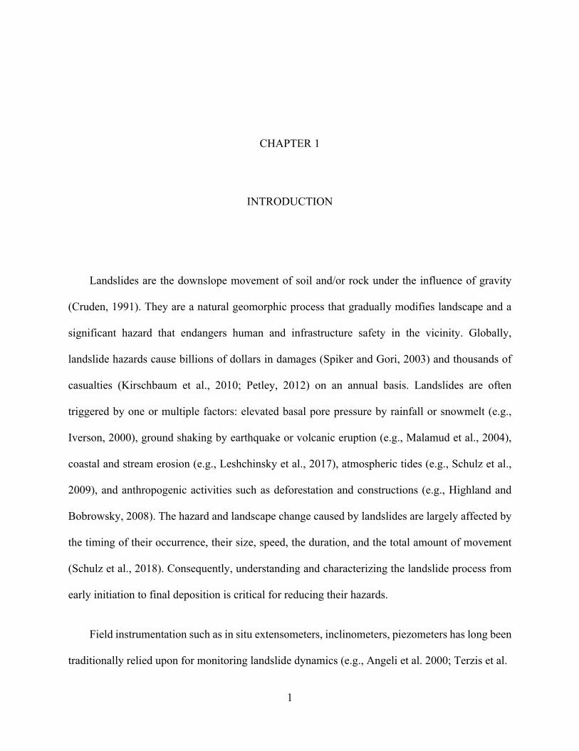
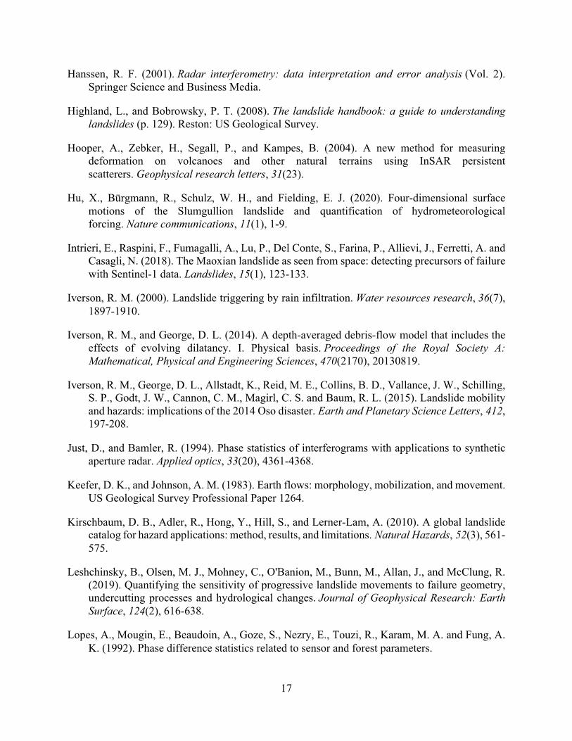
(Moreira et al., 2013). Figure 1.1a illustrates the typical SAR geometry, where the platform moves
in the azimuth direction and the slant-range direction is perpendicular to the radar’s flight path,
3
and the radar swath gives the ground-range of the radar scene. Because of the side-looking design,
the radar images are geometrically distorted from ground coordinate (Figure 1.1b) and a geocoding
processing is required to reproject the radar image into the ground coordinate.
Figure 1.1 Typical radar geometry and the resulted image distortion (after Rosen, 2000; Simons, 2005).
Imaging radar collects and forms a two-dimensional image composed of multiple lines and
columns of pixels. The slant-range resolution $# (pixel size along the range direction) of a radar
image is inversely proportional to the system bandwidth %# as
$# =&!2%#
(1.1)
where &! is the speed of light. The azimuth resolution -& depends on the length of radar antenna
.&:
-& =.&2(1.2)
4
The above equation suggests that a short antenna corresponds to a fine azimuth resolution,
which is because a radar with a shorter antenna “sees” any ground objects for a longer time
(Moreira et al., 2013). The illumination time can be approximated as
/$''( ≈12!3.&
(1.3)
where 1 is the wavelength of radar sensor, 2! is the distance between radar sensor and ground
objects, 3 is the moving speed of the platform along the azimuth direction.
The received echo signal is recorded as a two-dimensional data matrix in complex numbers
with a real in-phase component and an imaginary quadrature component, which can be converted
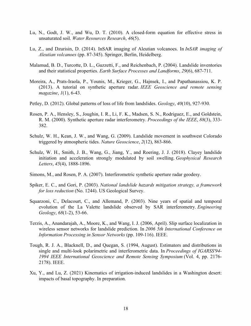
to amplitude and phase measures of the received echo. Unlike optical images, raw SAR images do
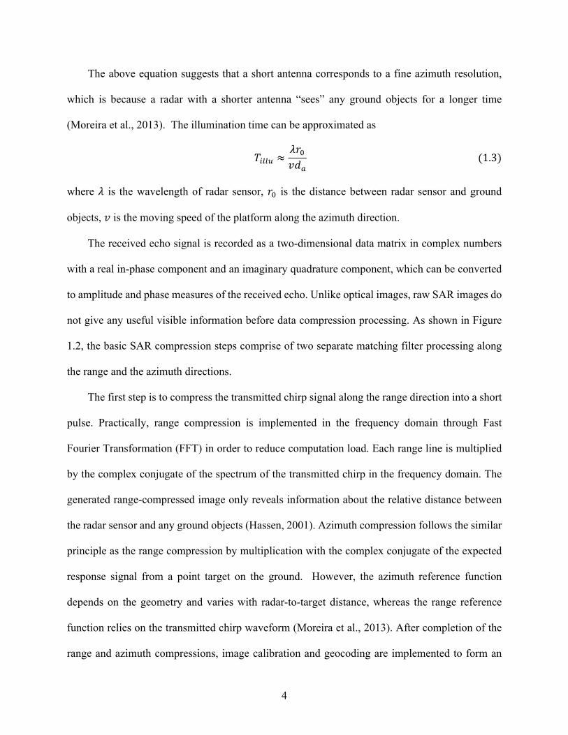
not give any useful visible information before data compression processing. As shown in Figure
1.2, the basic SAR compression steps comprise of two separate matching filter processing along
the range and the azimuth directions.
The first step is to compress the transmitted chirp signal along the range direction into a short
pulse. Practically, range compression is implemented in the frequency domain through Fast
Fourier Transformation (FFT) in order to reduce computation load. Each range line is multiplied
by the complex conjugate of the spectrum of the transmitted chirp in the frequency domain. The
generated range-compressed image only reveals information about the relative distance between
the radar sensor and any ground objects (Hassen, 2001). Azimuth compression follows the similar
principle as the range compression by multiplication with the complex conjugate of the expected
response signal from a point target on the ground. However, the azimuth reference function
depends on the geometry and varies with radar-to-target distance, whereas the range reference
function relies on the transmitted chirp waveform (Moreira et al., 2013). After completion of the
range and azimuth compressions, image calibration and geocoding are implemented to form an
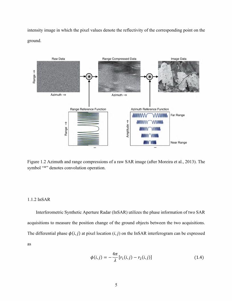
5
intensity image in which the pixel values denote the reflectivity of the corresponding point on the
ground.
Figure 1.2 Azimuth and range compressions of a raw SAR image (after Moreira et al., 2013). The symbol “*” denotes convolution operation.
1.1.2 InSAR
Interferometric Synthetic Aperture Radar (InSAR) utilizes the phase information of two SAR
acquisitions to measure the position change of the ground objects between the two acquisitions.
The differential phase 5(6, 8) at pixel location (6, 8) on the InSAR interferogram can be expressed
as
5(6, 8) = −4:1[2)(6, 8) − 2*(6, 8)](1.4)
6
where 2) and 2* are the slant ranges between the same ground object to the radar sensor in the first
and the second acquisition, respectively. The differential phase 5 comprises multiple
contributions:
5 = ={5+,-. + 5%./. + 5&%0 + 5.#1 + 52.$3,}(1.5)
where 5+,-., 5%./. , 5&%0, 5.#1 , and 52.$3, denote phases contributed by ground deformation,
topographic elevation change, atmospheric variation, orbital difference, signal noise between the
first and the second acquisition, and W{⋅} is the wrapping operator that drops whole phase cycles
(2π), as only a fractional part of a cycle can be measured with SAR interferometry. In order to
measure ground deformation 5+,-. from a SAR interferogram, other contributing terms must be
removed or suppressed.
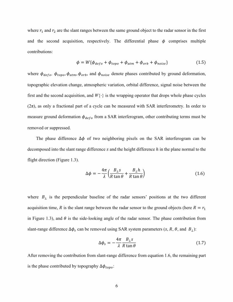
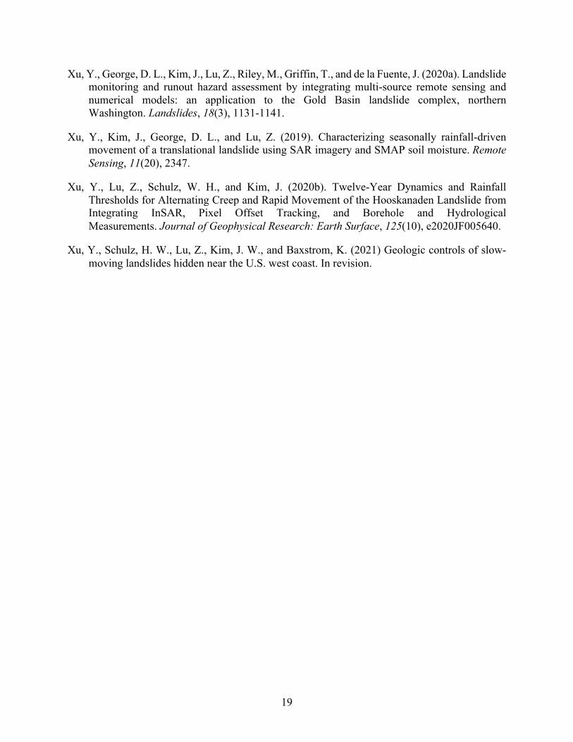
The phase difference Δ5 of two neighboring pixels on the SAR interferogram can be
decomposed into the slant range difference D and the height difference ℎ in the plane normal to the
flight direction (Figure 1.3).
Δ5 = −4:1F%4DG tan K
+%4ℎG tan K
L(1.6)
where %4 is the perpendicular baseline of the radar sensors’ positions at the two different
acquisition time, G is the slant range between the radar sensor to the ground objects (here G = 2)
in Figure 1.3), and K is the side-looking angle of the radar sensor. The phase contribution from
slant-range difference Δ53 can be removed using SAR system parameters (D, G, K, and %4):
Δ53 = −4:1
%4DG tan K
(1.7)
After removing the contribution from slant-range difference from equation 1.6, the remaining part
is the phase contributed by topography Δ5%./.:
7
Δ5%./. = Δ5 − Δ53 = −4:1
%4ℎG tan K
(1.8)
Therefore, if no deformation occurred between the two acquisitions, equation 1.8 can be used to
estimated topographic elevation on the earth surface. On the other hand, the topographic phase
contributions can be removed with given DEMs.
Figure 1.3 SAR interferometry imaging geometry in the plane normal to the flight direction (after Lu and Dzurisin, 2014).
The orbit-related artifacts 5.#1 can be simulated with the quadratic fitting (Fattahi and
Amelung, 2014). The stratified atmospheric artifacts related to regional topography can be reduced
by using a linear fitting, and other large-spatial-scale phase artifacts can be suppressed based on
polynomial fitting or weather models that estimate precipitable water content in the troposphere.
8
InSAR coherence is an indicator of the similarities of the backscattered signals in the two
acquisitions and reflects noise level of the InSAR phase. A moving-window cross-correlation
analysis is usually used to estimate the coherence P of two complex SAR images Q) and Q* (Lu
and Dzurisin, 2014; Lopes et al., 1992; Bamler and Just, 1993; Tough et al., 1994):
P =R[Q)Q*∗]
SR[|Q)|*]R[|Q*|*](1.9)
Where R[∙] denotes the expectation value that in practice will be approximated with a sampled
average (Lopes et al., 1992; Just and Bamler, 1994; Anxi et al., 2014).
The above-described contents introduce the steps to generate one single interferogram from
two SAR acquisitions. With multiple InSAR pairs available, the multi-temporal processing such
as Permanent scatterer InSAR (PS-InSAR; Ferretti et al., 2001; Hooper, 2004) and small baseline
subset (SBAS) InSAR (Berardino et al., 2002) can be implemented to retrieve deformation time
series of ground objects.
1.2 Landslide Processes
In a full life cycle from early initiation to final deposition, landslides undergo one or multiple
rounds of acceleration-deceleration movements. Catastrophic landslides usually experience abrupt
failure followed by rapid downslope motion and start to slow down upon hitting flat or uphill
grounds to reach final deposition (Highland and Bobrowsky, 2008). The entire process may only
include one acceleration-deceleration cycle. In contrast, many reactivated clayey landslides
undergo multiple acceleration-deceleration cycles characterized by slow motions which are often
associated with seasonal precipitation (e.g., Keefer and Johnson, 1983). Nonetheless, both types
9
of post-failure movements follow Newton’s Law of Motion and the landslide initiation follows the
Mohr-Coulomb shearing failure criteria:
W'$0 = & + -,XYZ[(1.10)
where W'$0 is the limit shear strength, & the effective cohesion, [ the internal friction angle. The
effective stress -, is defined as (Lu et al., 2010)
-, = - − Q& − [−K,(Q& − Q6)](1.11)
where - is the normal stress component of gravity, Q& the atmospheric pressure, Q6 the water
pressure, and K, the effective saturation. Landslide instigates when the basal shear stress exceeds
the material’s shear strength.
Once slope failures instigate, their subsequent post-failure behaviors may vary depending on
basal topography, soil contraction/dilation, and external stress inputs. Contractive landslide
materials on a steep slope tend to evolve into rapid debris flows by constantly gaining movement
momentum, whereas dilative materials on a gentle slope may quickly slow down if without extra
pushing stress such as rainfall. Fundamentally, landslide motions obey the principles of classical
mechanics such as conservation of mass and conservation of momentum.
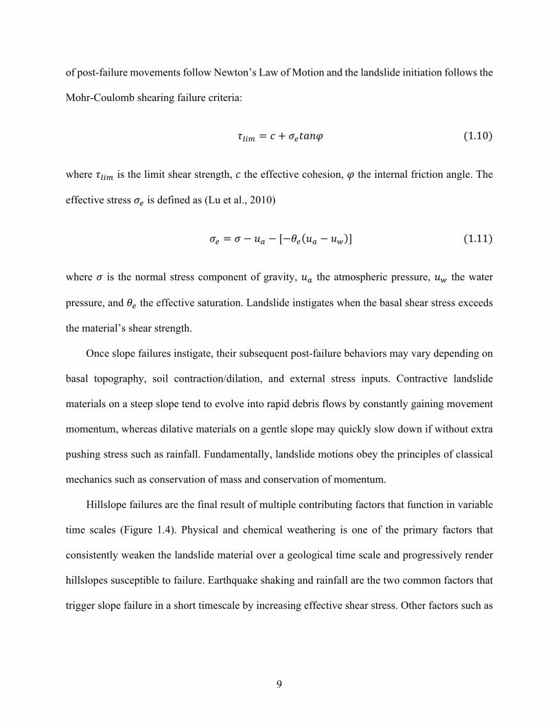
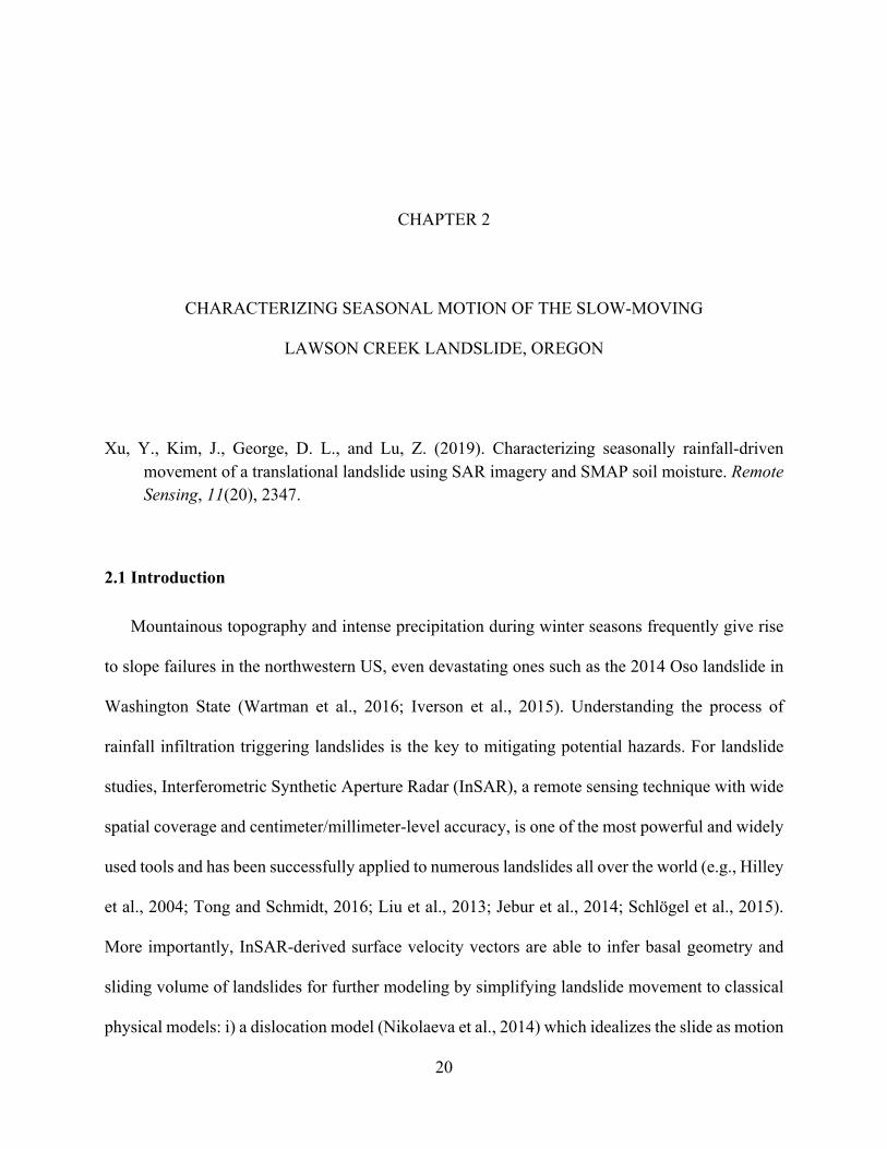
Hillslope failures are the final result of multiple contributing factors that function in variable
time scales (Figure 1.4). Physical and chemical weathering is one of the primary factors that
consistently weaken the landslide material over a geological time scale and progressively render
hillslopes susceptible to failure. Earthquake shaking and rainfall are the two common factors that
trigger slope failure in a short timescale by increasing effective shear stress. Other factors such as
10
stream erosion of the landslide toe and extra loading at the landslide head could also alter the stress
regime and shift a stable hillslope into failure.
Capturing landslide kinematics using remote sensing helps to understand landslide behaviors
under variable internal and external forcing (e.g., Hu et al., 2020) and to generate insights for
forecasting potential future hazards of unstable hillslopes (e.g., Intrieri et al., 2018).
Figure 1.4 Stress regime evolution of a landslide over time. Landslide failure occurs when the shear stress exceeds the shear strength. X), X*, X7 denote the time.
1.3 Chapter Summarizes and Contributions
Chapters 2, 3, 4, 5, and 6 are written for peer-reviewed publication. Chapters 2 – 4 includes
my research published in three journals: Remote Sensing (Xu et al., 2019), Landslides (Xu et al.,
2020a), and Journal of Geophysical Research: Earth Surface (Xu et al., 2020b). Chapter 5 is
submitted to a peer-reviewed journal Landslides (Xu et al., 2021a). Chapter 6 is part of a
manuscript which is in preparation for submission to a peer-reviewed journal (Xu et al., 2021b).
Chapter 7 highlights the findings of the dissertation and discusses topics of future work.
11
Chapter 2: This chapter presents a case study of the constantly slow-moving Lawson Creek
landslide in southwestern Oregon, where InSAR, space-sensed soil moisture, and thickness
inversion and hydromechanical models were used to characterize the landslide motion dynamics
(Xu et al., 2019). Typical of most slow-moving landslides, precipitation infiltrates into basal
shearing zones and triggers seasonal landslide motion by increasing pore-pressure and reducing
shear resistance. This process is jointly controlled by basal depth, rainfall intensity, soil moisture,
and hydraulic conductivity/diffusivity. Using interferometric synthetic aperture radar (InSAR), we
detected and mapped a typical slow-moving landslide in the southwestern Oregon – the Lawson
Creek landslide. Its basal depths are estimated using InSAR derived pseudo-3D surface velocity
fields based on the mass conservation approach by assuming a power-law rheology. The estimated
maximum thickness over the central region of the landslide is 6.9 ± 2.6 m, and this result is further
confirmed by an independent limit equilibrium analysis that solely relies on soil mechanical
properties. By incorporating satellites-captured time lags of 27 – 49 days between the onset of wet
seasons and the initiation of landslide motions, we estimated the averaged characteristic hydraulic
conductivity and diffusivity of the landslide material as 1.2 × 10⁻⁵ m/s and 1.9 × 10⁻⁴ m2/s,
respectively. This investigation laid out a framework for using InSAR and satellite-sensed soil
moisture to infer landslide basal geometry and estimate corresponding hydraulic parameters.
Chapter 3: This chapter provides a case study of the alternatingly slow and rapidly moving
Hooskanaden landslide in the southern Oregon coast, where multi-sensor remote sensing (LiDAR,
InSAR, and optical images) and one-dimensional rainfall infiltration and pore pressure diffusion
models were integrated to obtain 3D landslide surface motions, and to derive physics-based rainfall
thresholds for the observed contrasting landslide motion behaviors (Xu et al., 2020b). The
Hooskanaden landslide is a large (~600 m wide × 1,300 m long), deep (~30 – 45 m) slide located
12
in southwestern Oregon. Since 1958, it has had five moderate/major movements that
catastrophically damaged the intersecting U.S. Highway 101, along with persistent slow wet‐
season movements and a long‐term accelerating trend due to coastal erosion. Multiple remote
sensing approaches, borehole measurements, and hydrological observations have been integrated
to interpret the motion behaviors of the slide. Pixel offset tracking of both Sentinel‐1 and Sentinel‐
2 images was carried out to reconstruct the 3D displacement field of the 2019 major event, and the
results agree well with field measurements. A 12‐year displacement history of the landslide from
2007 to 2019 has been retrieved by incorporating offsets from LiDAR DEM gradients and InSAR
processing of ALOS and Sentinel‐1 images. Comparisons with daily/hourly ground precipitation
reveal that the motion dynamics are predominantly controlled by intensity and temporal pattern of
rainfall. A new empirical threefold rainfall threshold was therefore proposed to forecast the dates
for the moderate/major movements. This threshold relies upon antecedent water‐year and previous
3‐day and daily precipitation, and was able to represent observed movement periods well.
Adaptation of our threshold methodology could prove useful for other large, deep landslides for
which temporal forecasting has long been generally intractable. The averaged characteristic
hydraulic conductivity and diffusivity were estimated as 6.6 × 10⁻⁶ m/s and 6.6 × 10⁻⁴ m2/s,
respectively, based on the time lags between rainfall pulses and slide accelerations. The ability of
the new rainfall threshold was explained by hydrologic modeling.
Chapter 4: This chapter shows a case study of a potentially catastrophic landslide – the Gold
Basin landslide complex in northern Washington, where multisource remote sensing approaches
(LiDAR DEM differencing, sub-pixel offset tracking, and InSAR) and the D-claw runout model
(Iverson and George, 2014; George and Iverson, 2014) were employed to monitor recent landslide
activities and estimate potential inundation zones upon a hypothetical catastrophic failure (Xu et
13
a., 2020a). The landslide complex at Gold Basin, Washington, has been drawing considerable
attention after a catastrophic runout of the nearby landslide at Oso, Washington, in 2014. To
evaluate potential threats of the Gold Basin landslide to the campground down the slope, remote
sensing and numerical modeling were integrated to monitor recent landslide activity and simulate
hypothetical runout scenarios. Bare-earth LiDAR DEM differencing, InSAR, and offset tracking
of SAR images reveal that localized collapses at the headscarps have been the primary type of
landslide activity at Gold Basin from 2005 to 2019, and currently no signs indicative of movement
of a large, centralized block or a deep-seated main body were detected. The maximum horizontal
deformation rate is 5 m/year occurring primarily from headscarp recession of the middle lobe, and
the annual landsliding volume of the whole landslide complex averages 1.03 × 10⁵ m3. From three-
dimensional limit equilibrium analysis of generalized terrace structures, the maximum landslide
volume is estimated as 2.0 × 10⁶ m3. Simulations of hypothetical runout scenarios were carried out
using the depth-averaged two-phase model D-claw with above-obtained landslide geometry
constraints. The simulation results demonstrate that debris flows with volume less than 105 m3
only pose limited threats to the campground, while volumes over 106 m3 could cause severe
damages. Consequently, the estimated maximum landslide volume of 2.0 × 10⁶ m3 suggests a
potential risk to the campground nearby. In addition, our simulations of a river at the landslide toe
demonstrate that interactions between debris flow and waterbodies could impact the flow
kinematics considerably depending on flow speed, waterbody volume, and topographical settings.
This study provided a useful methodology for evaluating other similar landslides globally for
hazards prevention and mitigation.
Chapter 5: This chapter is focused on discovering slow-moving landslides near the United States
west coast and investigating their geologic controls from bedrock lithology and land uplift (Xu et
14
al., 2021). Slow-moving landslides, often with nearly imperceptible creeping motion, are an
important landscape shaper and a dangerous natural hazard across the globe, yet their spatial
distribution and geologic controls are still poorly known owing to a paucity of detailed, large-scale
observations. Here we use interferometry of L-band satellite radar images to reveal 630 spatially
large (4×10⁴ – 13×106 m2) and presently active (2007–2019) slow-moving landslides hidden near
the populous United States west coast (only 4.6% of these slides were previously known) and
provide evidence for their fundamental controls by bedrock lithology and vertical land motion. We
found that slow-moving landslides are generally larger and more spatially frequent in
homogeneous bedrock with low rock strength, and they are preferentially located on hillslopes
with geologically recent uplift. Notably, landslide size and spatial density in the relatively weak
metamorphic rocks and mélange (due to pervasive tectonically sheared discontinuities, foliation,
and abundant clay minerals) were two times larger than those in sedimentary and igneous rocks,
and the hillslopes with landslides were found to be uplifting approximately three times faster than
the average for the whole region. These analysis suggests that occurrence and character of slow-
moving landslides may be anticipated from vertical land motion rates and bedrock lithology.
Hence, this study provides understanding critical for reducing landslide hazards and quantifying
landslide impacts on landscape change.
Chapter 6: This chapter presents a case study of irrigation-triggered landslides in a Washington
dessert and their motion kinematics regulated by basal topography (Xu and Lu, 2021). Landslides
are usually a natural geomorphic process, while anthropogenic activities such as agricultural
irrigation in semiarid regions could produce widespread landslides which damage infrastructures,
endanger safety of local residents, and cause considerable ecological prices. Here we utilized both
satellite optical and radar images acquired between 1996 and 2020 to identify 13 slow landslide
15
complexes and 12 catastrophic landslides which were triggered by excessive irrigation water in a
Washington dessert near Hanford. InSAR time-series displacements of seven slow landslides
reveal that riverside landslides were strongly modulated by water level of the Columbia River
where the landslide toes reside, yet their seasonal instigation and cessation were not controlled by
a single fixed groundwater level threshold. Our numerical modeling shows that such phenomenon
could be explained by the forced water circulation on an irregular slip surface where accelerated
landslide velocity increases the upslope resistance and consequently contributes to slowing down
the landslide body. By integrating satellite observations of two highly similar slow landslides, we
characterized the life cycle of slow landslides in the region as a rapid acceleration to the peak rate
within 3 years followed by a slow deceleration in exponentially decreasing rates for about 40 years.
In addition, comparison of longitudinal topographical profiles of five typical slow landslides and
five catastrophic landslides demonstrates that steep basal surface and runout path are more likely
to produce catastrophic landslides with a long runout due to rapid kinetic energy gain during the
movement. Basal topography of slow landslides at particularly the toe section exerts critical
impacts on their motion evolution. Our investigation provides understandings critical for
characterizing motion dynamics of both slow and catastrophic landslides with irregular basal
surfaces, and therefore is widely applicable to many landslides globally for hazard reduction.
Chapter 7: This chapter provides conclusions and discusses future work.
16
REFERENCES
Angeli, M. G., Pasuto, A., and Silvano, S. (2000). A critical review of landslide monitoring experiences. Engineering Geology, 55(3), 133-147.
Anxi, Y., Haijun, W., Zhen, D., and Haifeng, H. (2014). Amplitude and phase statistics of multi-look SAR complex interferogram. Defence Science Journal, 64(6), 564.
Bamler, R., and Just, D. (1993, August). Phase statistics and decorrelation in SAR interferograms. In Proceedings of IGARSS'93-IEEE International Geoscience and Remote Sensing Symposium (pp. 980-984). IEEE.
Berardino, P., Fornaro, G., Lanari, R., and Sansosti, E. (2002). A new algorithm for surface deformation monitoring based on small baseline differential SAR interferograms. IEEE Transactions on geoscience and remote sensing, 40(11), 2375-2383.
Colesanti, C., and Wasowski, J. (2006). Investigating landslides with space-borne Synthetic Aperture Radar (SAR) interferometry. Engineering geology, 88(3-4), 173-199.
Cruden, D. M. (1991). A simple definition of a landslide. Bulletin of the International Association of Engineering Geology-Bulletin de l'Association Internationale de Géologie de l'Ingénieur, 43(1), 27-29.
Fattahi, H., and Amelung, F. (2014). InSAR uncertainty due to orbital errors. Geophysical Journal International, 199(1), 549-560.
Ferretti, A., Prati, C., and Rocca, F. (2001). Permanent scatterers in SAR interferometry. IEEE Transactions on geoscience and remote sensing, 39(1), 8-20.
Fruneau, B., Achache, J., and Delacourt, C. (1996). Observation and modelling of the Saint-Etienne-de-Tinée landslide using SAR interferometry. Tectonophysics, 265(3-4), 181-190.
George, D. L., and Iverson, R. M. (2014). A depth-averaged debris-flow model that includes the effects of evolving dilatancy. II. Numerical predictions and experimental tests. Proceedings of the Royal Society A: Mathematical, Physical and Engineering Sciences, 470(2170), 20130820.
17
Hanssen, R. F. (2001). Radar interferometry: data interpretation and error analysis (Vol. 2). Springer Science and Business Media.
Highland, L., and Bobrowsky, P. T. (2008). The landslide handbook: a guide to understanding landslides (p. 129). Reston: US Geological Survey.
Hooper, A., Zebker, H., Segall, P., and Kampes, B. (2004). A new method for measuring deformation on volcanoes and other natural terrains using InSAR persistent scatterers. Geophysical research letters, 31(23).
Hu, X., Bürgmann, R., Schulz, W. H., and Fielding, E. J. (2020). Four-dimensional surface motions of the Slumgullion landslide and quantification of hydrometeorological forcing. Nature communications, 11(1), 1-9.
Intrieri, E., Raspini, F., Fumagalli, A., Lu, P., Del Conte, S., Farina, P., Allievi, J., Ferretti, A. and Casagli, N. (2018). The Maoxian landslide as seen from space: detecting precursors of failure with Sentinel-1 data. Landslides, 15(1), 123-133.
Iverson, R. M. (2000). Landslide triggering by rain infiltration. Water resources research, 36(7), 1897-1910.
Iverson, R. M., and George, D. L. (2014). A depth-averaged debris-flow model that includes the effects of evolving dilatancy. I. Physical basis. Proceedings of the Royal Society A: Mathematical, Physical and Engineering Sciences, 470(2170), 20130819.
Iverson, R. M., George, D. L., Allstadt, K., Reid, M. E., Collins, B. D., Vallance, J. W., Schilling, S. P., Godt, J. W., Cannon, C. M., Magirl, C. S. and Baum, R. L. (2015). Landslide mobility and hazards: implications of the 2014 Oso disaster. Earth and Planetary Science Letters, 412, 197-208.
Just, D., and Bamler, R. (1994). Phase statistics of interferograms with applications to synthetic aperture radar. Applied optics, 33(20), 4361-4368.
Keefer, D. K., and Johnson, A. M. (1983). Earth flows: morphology, mobilization, and movement. US Geological Survey Professional Paper 1264.
Kirschbaum, D. B., Adler, R., Hong, Y., Hill, S., and Lerner-Lam, A. (2010). A global landslide catalog for hazard applications: method, results, and limitations. Natural Hazards, 52(3), 561-575.
Leshchinsky, B., Olsen, M. J., Mohney, C., O'Banion, M., Bunn, M., Allan, J., and McClung, R. (2019). Quantifying the sensitivity of progressive landslide movements to failure geometry, undercutting processes and hydrological changes. Journal of Geophysical Research: Earth Surface, 124(2), 616-638.
Lopes, A., Mougin, E., Beaudoin, A., Goze, S., Nezry, E., Touzi, R., Karam, M. A. and Fung, A. K. (1992). Phase difference statistics related to sensor and forest parameters.
18
Lu, N., Godt, J. W., and Wu, D. T. (2010). A closed‐form equation for effective stress in unsaturated soil. Water Resources Research, 46(5).
Lu, Z., and Dzurisin, D. (2014). InSAR imaging of Aleutian volcanoes. In InSAR imaging of Aleutian volcanoes (pp. 87-345). Springer, Berlin, Heidelberg.
Malamud, B. D., Turcotte, D. L., Guzzetti, F., and Reichenbach, P. (2004). Landslide inventories and their statistical properties. Earth Surface Processes and Landforms, 29(6), 687-711.
Moreira, A., Prats-Iraola, P., Younis, M., Krieger, G., Hajnsek, I., and Papathanassiou, K. P. (2013). A tutorial on synthetic aperture radar. IEEE Geoscience and remote sensing magazine, 1(1), 6-43.
Petley, D. (2012). Global patterns of loss of life from landslides. Geology, 40(10), 927-930.
Rosen, P. A., Hensley, S., Joughin, I. R., Li, F. K., Madsen, S. N., Rodriguez, E., and Goldstein, R. M. (2000). Synthetic aperture radar interferometry. Proceedings of the IEEE, 88(3), 333-382.
Schulz, W. H., Kean, J. W., and Wang, G. (2009). Landslide movement in southwest Colorado triggered by atmospheric tides. Nature Geoscience, 2(12), 863-866.
Schulz, W. H., Smith, J. B., Wang, G., Jiang, Y., and Roering, J. J. (2018). Clayey landslide initiation and acceleration strongly modulated by soil swelling. Geophysical Research Letters, 45(4), 1888-1896.
Simons, M., and Rosen, P. A. (2007). Interferometric synthetic aperture radar geodesy.
Spiker, E. C., and Gori, P. (2003). National landslide hazards mitigation strategy, a framework for loss reduction (No. 1244). US Geological Survey.
Squarzoni, C., Delacourt, C., and Allemand, P. (2003). Nine years of spatial and temporal evolution of the La Valette landslide observed by SAR interferometry. Engineering Geology, 68(1-2), 53-66.
Terzis, A., Anandarajah, A., Moore, K., and Wang, I. J. (2006, April). Slip surface localization in wireless sensor networks for landslide prediction. In 2006 5th International Conference on Information Processing in Sensor Networks (pp. 109-116). IEEE.
Tough, R. J. A., Blacknell, D., and Quegan, S. (1994, August). Estimators and distributions in single and multi-look polarimetric and interferometric data. In Proceedings of IGARSS'94-1994 IEEE International Geoscience and Remote Sensing Symposium (Vol. 4, pp. 2176-2178). IEEE.
Xu, Y., and Lu, Z. (2021) Kinematics of irrigation-induced landslides in a Washington desert: impacts of basal topography. In preparation.
19
Xu, Y., George, D. L., Kim, J., Lu, Z., Riley, M., Griffin, T., and de la Fuente, J. (2020a). Landslide monitoring and runout hazard assessment by integrating multi-source remote sensing and numerical models: an application to the Gold Basin landslide complex, northern Washington. Landslides, 18(3), 1131-1141.
Xu, Y., Kim, J., George, D. L., and Lu, Z. (2019). Characterizing seasonally rainfall-driven movement of a translational landslide using SAR imagery and SMAP soil moisture. Remote Sensing, 11(20), 2347.
Xu, Y., Lu, Z., Schulz, W. H., and Kim, J. (2020b). Twelve‐Year Dynamics and Rainfall Thresholds for Alternating Creep and Rapid Movement of the Hooskanaden Landslide from Integrating InSAR, Pixel Offset Tracking, and Borehole and Hydrological Measurements. Journal of Geophysical Research: Earth Surface, 125(10), e2020JF005640.
Xu, Y., Schulz, H. W., Lu, Z., Kim, J. W., and Baxstrom, K. (2021) Geologic controls of slow- moving landslides hidden near the U.S. west coast. In revision.
20
CHAPTER 2
CHARACTERIZING SEASONAL MOTION OF THE SLOW-MOVING
LAWSON CREEK LANDSLIDE, OREGON
Xu, Y., Kim, J., George, D. L., and Lu, Z. (2019). Characterizing seasonally rainfall-driven movement of a translational landslide using SAR imagery and SMAP soil moisture. Remote Sensing, 11(20), 2347.
2.1 Introduction
Mountainous topography and intense precipitation during winter seasons frequently give rise
to slope failures in the northwestern US, even devastating ones such as the 2014 Oso landslide in
Washington State (Wartman et al., 2016; Iverson et al., 2015). Understanding the process of
rainfall infiltration triggering landslides is the key to mitigating potential hazards. For landslide
studies, Interferometric Synthetic Aperture Radar (InSAR), a remote sensing technique with wide
spatial coverage and centimeter/millimeter-level accuracy, is one of the most powerful and widely
used tools and has been successfully applied to numerous landslides all over the world (e.g., Hilley
et al., 2004; Tong and Schmidt, 2016; Liu et al., 2013; Jebur et al., 2014; Schlögel et al., 2015).
More importantly, InSAR-derived surface velocity vectors are able to infer basal geometry and
sliding volume of landslides for further modeling by simplifying landslide movement to classical
physical models: i) a dislocation model (Nikolaeva et al., 2014) which idealizes the slide as motion
21
on a rectangular planar basal surface assuming elastic sliding materials; ii) a cross-section method
(Aryal et al., 2015) which regards a landslide as a set of independent cross-sections and ignores
the connection between adjacent blocks; iii) a mass conservation approach which assumes that
sliding materials have homogeneous rheological properties and are incompressible (Booth et al.,
2013). These simplified models vary in accuracy depending on both the particular landslide
behavior and the InSAR derived displacement vectors.
Elevated basal pore-fluid pressure through rainwater infiltration is considered the primary
trigger for seasonal landslides by weakening the soil’s resistive strength (Iverson et al., 1987; Reid,
1994; Baum and Reid, 1995; Bogaard and Greco, 2016). Pore pressure transmission in saturated
soils approximates a diffusive process depending on hydraulic diffusivity (Berti and Simoni, 2010;
Iverson, 2000), yet basal pore-water’s pressure response to precipitation in post-summer
unsaturated soils is strongly affected by water infiltration rates (advective flow) that rely on
hydraulic conductivity. Therefore, landslide geometry, soil properties and the initial soil moisture
jointly control the response time of slope failure to seasonal precipitation. Nevertheless, the
characteristic hydraulic parameters can be quatified if the failure depth and the water infiltration
time are known.
Using SAR imagery from three spaceborne radar systems including Advanced Land
Observing Satellite (ALOS) Phased Array type L-band synthetic aperture radar (PALSAR),
ALOS-2 PALSAR-2 and Sentinel-1A/B, we detected a slow-moving landslide in southern Oregon
and mapped its time-series deformation from 2007 to 2011 and 2016 to 2018. The basal depth and
volume of the landslide are estimated using InSAR-derived surface velocity fields and the mass
conservation approach (Rutt et al., 2009; Booth et al., 2013). The limit equilibrium analysis is
implemented to validate the estimated failure depth. By incorporating the failure depth and derived
22
time lags between the arrival of wet seasons and the initiation of seasonally landslide motions
using InSAR and satellite soil moisture from SMAP (Soil Moisture Active and Passive), we
estimated the lower and upper bounds of characteristic hydraulic conductivity and diffusivity of
the landslide material.
2.2 Landslide Location and Geological Settings
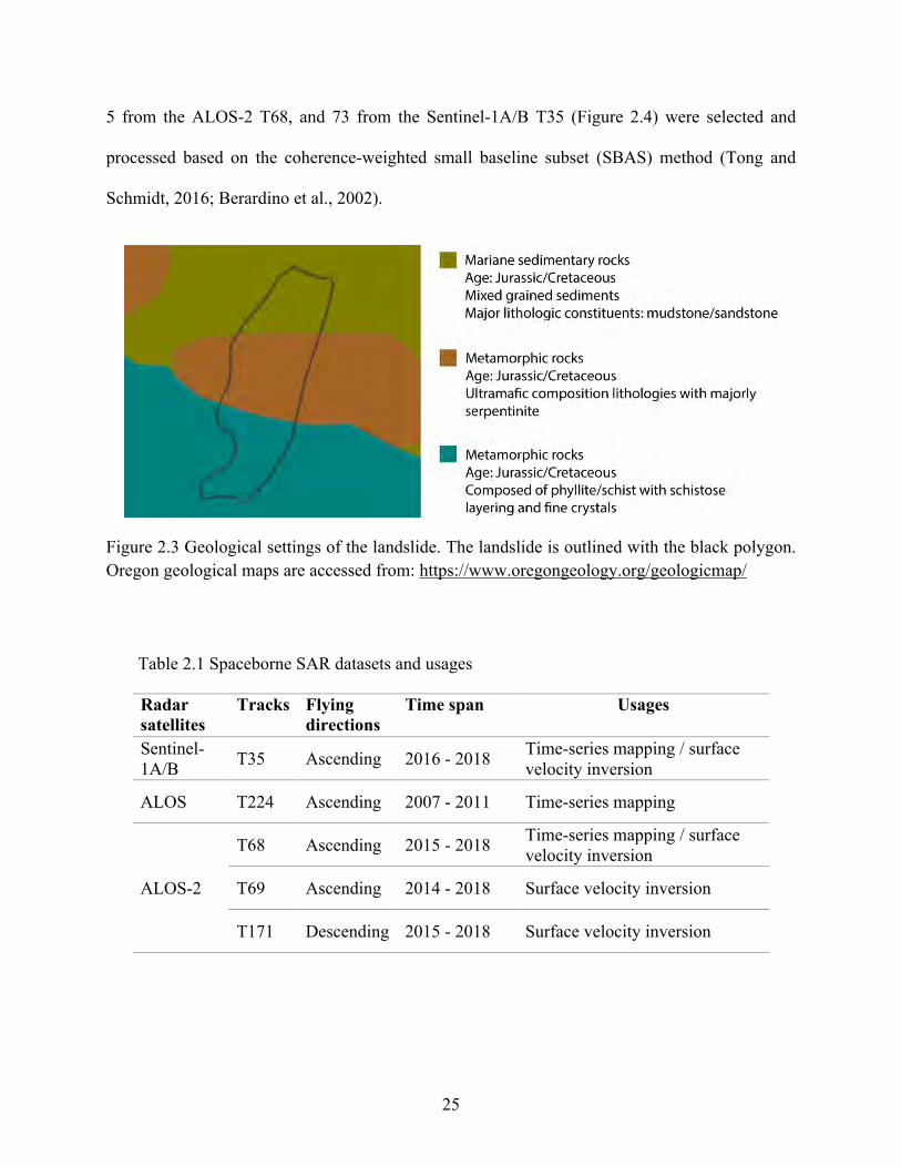
The Lawson Creek landslide is a slow-moving translational landslide located in southwestern
Oregon with a ~1.5 km long and ~500 m wide sliding body (Figure 2.1). The slope faces northwest
with an aspect of ~294° clockwise from north, and the average slope is ~10°. There are no obvious
scarps near the landslide’s head as it has been seated on deposits of a previous landslide, and the
currently active slide is only a small part of the ancient landslide deposits mapped in the Statewide
Landslide Information Database for Oregon (SLIDO (Burns, 2014); Figure 2.2). The bedrock of
the slide is composed of marine sedimentary rocks with sandstone/mudstone lithologies at the
upper section, metamorphic rocks with majorly serpentine at the middle section, and metamorphic
rocks with phyllite/schist lithologies at the lower section (Figure 2.3). The toe of the landslide
enters Lawson Creek at an elevation of 358 m, and its crown stands at 610 m. The primary
precipitation in this region falls between mid-October and mid-April, while little rainfall comes in
other months. Moderately dense vegetation covers the landslide site.
2.3 Materials and Methods
2.3.1 SAR Interferometry for Landslide Time-series Mapping
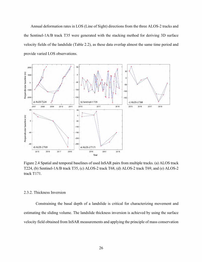
SAR imagery from the ALOS ascending track T224, ALOS-2 ascending tracks T68 and T69
and descending track T171, and the Sentinel-1A/B ascending track T35 were used to map
displacements of the Lawson Creek landslide (Figure 2.1; Table 2.1). The 1-acrsec Shuttle Radar
23
Topography Mission (SRTM) Digital Elevation Model (DEM) obtained from U.S. Geological
Survey (USGS) was used in the InSAR processing. Baseline error and stratified atmospheric
artifacts were removed before phase unwrapping. The GAMMA software (Werner et al., 2002)
was used for interferogram generation, phase unwrapping, and removal of stratified atmospheric
artifacts. Unwrapping errors in a few interferograms caused by high-gradient sliding movements
were corrected by separating the original wrapped phase into an estimated high-gradient
displacement component and a residual-phase component (within 2π variation). We unwrapped
only the residual-phase component and added it back to the estimated high-gradient component to
obtain the final unwrapped phase. The high-gradient displacement component was estimated based
on interferograms with short temporal baselines and very good coherences. Manual check is
required to confirm the corrections. The corrected interferograms have been listed in the
supplementary table in Xu et al. 2019.
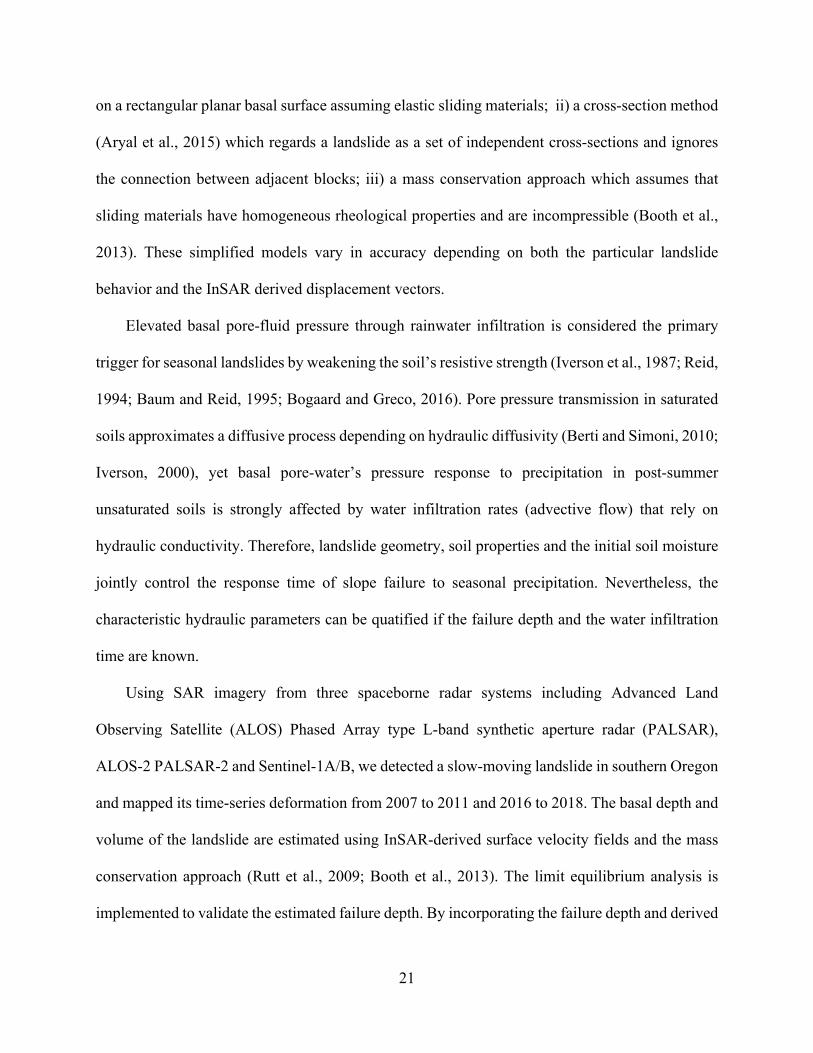
Figure 2.1 Geographical location of the Lawson Creek landslide and SAR data used in this study. The landslide (marked with a red star) is located in Curry county, southwestern Oregon, about 27
24
km inland from the Pacific Ocean. The location of Oregon is outlined in blue in both scaled-down (top-left corner) and scaled-up (bottom-left corner) maps. The red box at the bottom-left-corner figure represents geographical location of the whole Figure 1, and the magenta point represents a ground reference site for soil-moisture measurements (Miller Woods station). The red diamond near the landslide site represents a precipitation collection site (Agness station). SAR imagery covering the landslide is denoted with colored rectangular boxes annotated by track names in corresponding colors. The background shaded relief map was accessed from U.S. Geological Survey.
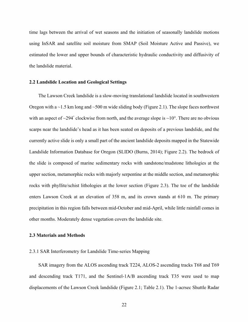
Figure 2.2 Historic landslide deposits. (a) The red pattern-filled polygon denotes an ancient (>150 years) deep-seated (> 4.5 m) landslide deposit. The yellow polygon outlines the actively deforming region captured by InSAR from 2007 to 2018. (b) Landslides view from optical remote sensing. The background RGB image was obtained in June 2019.
SAR acquisitions from the ALOS T224 and the Sentinel-1A/B T35 were used to generate
time-series displacement maps of the landslide, as they provide temporally dense and coherent
observations that allow construction of a fully connected network for time-series inversions
(Figure 2.4). To verify the C-band sentinel-1A/B time series measurements, we also produced
results using the L-band ALOS-2 T68 images spanning the same time period (Figure 2.6d). The
full set of interferograms that contain moderate or better coherence (over 0.2 for C-band data and
over 0.4 for L-band data) were used for time-series maps: 36 interferograms from the ALOS T224,
25
5 from the ALOS-2 T68, and 73 from the Sentinel-1A/B T35 (Figure 2.4) were selected and
processed based on the coherence-weighted small baseline subset (SBAS) method (Tong and
Schmidt, 2016; Berardino et al., 2002).
Figure 2.3 Geological settings of the landslide. The landslide is outlined with the black polygon. Oregon geological maps are accessed from: https://www.oregongeology.org/geologicmap/
Table 2.1 Spaceborne SAR datasets and usages
Radar satellites
Tracks Flying directions
Time span Usages
Sentinel-1A/B
T35 Ascending 2016 - 2018 Time-series mapping / surface velocity inversion
ALOS T224 Ascending 2007 - 2011 Time-series mapping
ALOS-2
T68 Ascending 2015 - 2018 Time-series mapping / surface velocity inversion
T69 Ascending 2014 - 2018 Surface velocity inversion
T171 Descending 2015 - 2018 Surface velocity inversion
26
Annual deformation rates in LOS (Line of Sight) directions from the three ALOS-2 tracks and
the Sentinel-1A/B track T35 were generated with the stacking method for deriving 3D surface
velocity fields of the landslide (Table 2.2), as these data overlap almost the same time period and
provide varied LOS observations.
Figure 2.4 Spatial and temporal baselines of used InSAR pairs from multiple tracks. (a) ALOS track T224, (b) Sentinel-1A/B track T35, (c) ALOS-2 track T68, (d) ALOS-2 track T69, and (e) ALOS-2 track T171.
2.3.2. Thickness Inversion
Constraining the basal depth of a landslide is critical for characterizing movement and
estimating the sliding volume. The landslide thickness inversion is achieved by using the surface
velocity field obtained from InSAR measurements and applying the principle of mass conservation
27
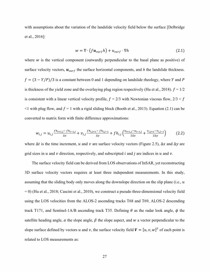
with assumptions about the variation of the landslide velocity field below the surface [Delbridge
et al., 2016]:
] = ∇ ∙ _`a3(#-ℎb + Q3(#- ⋅ ∇ℎ(2.1)
where ] is the vertical component (outwardly perpendicular to the basal plane as positive) of
surface velocity vectors, a3(#- the surface horizontal components, and ℎ the landslide thickness.
` = (3 − c/e)/3 is a constant between 0 and 1 depending on landslide rheology, where c and e
is thickness of the yield zone and the overlaying plug region respectively (Hu et al., 2018). ` = 1/2
is consistent with a linear vertical velocity profile, ` = 2/3 with Newtonian viscous flow, 2/3 < `
<1 with plug flow, and ` = 1 with a rigid sliding block (Booth et al., 2013). Equation (2.1) can be
converted to matrix form with finite difference approximations:
]$,9 = Q$,9-:!"#,%; -:!&#,%
∆=+ 3$,9
-:!,%"#; -:!,%&#∆>
+ `ℎ$,9 f(!"#,%;(!&#,%
*∆=+
?!,%"#;?!,%&#*∆>
g(2.2)
where ∆X is the time increment, Q and 3 are surface velocity vectors (Figure 2.5), ∆i and ∆j are
grid sizes in Q and 3 direction, respectively, and subscripted 6 and 8 are indices in Q and 3.
The surface velocity field can be derived from LOS observations of InSAR, yet reconstructing
3D surface velocity vectors requires at least three independent measurements. In this study,
assuming that the sliding body only moves along the downslope direction on the slip plane (i.e., Q
= 0) (Hu et al., 2018; Cascini et al., 2010), we construct a pseudo three-dimensional velocity field
using the LOS velocities from the ALOS-2 ascending tracks T68 and T69, ALOS-2 descending
track T171, and Sentinel-1A/B ascending track T35. Defining K as the radar look angle, 5 the
satellite heading angle, k the slope angle, l the slope aspect, and ] a vector perpendicular to the
slope surface defined by vectors Q and 3, the surface velocity field m = [Q, 3, ]]@ of each point is
related to LOS measurements as:
28
n o&Ap ∙ D ∙ m = qrst
0u(2.3)
where o = [v), v*, v7, ⋯ vB ]@ is the radar look vector of x independent LOS observations, and v) =
v* =⋯ = vB = [− sin K sin5 sin K cos5 − cos5]@,&A = [− sin lcos l0] is the
constrain condition, rst is the x independent InSAR measurements, and D is a coordinate
transformation matrix:
D = }cos l cos ksin l cos k − sin k− sin l cos l0cos l sin k sin l sin k cos k
~(2.4)
We solve Equation (2.3) to obtain the pseudo 3D surface velocity vectors with the least squares
approach, and solve Equation (2.2) for ℎ by using a nonnegative least squares method (Booth et
al., 2013; Grant et al., 2008) and setting boundary conditions that the landslide’s thicknesses range
from 0 to 200 m and non-landslide regions have a thickness of zero.
2.3.3 Time Lags
The initiation of seasonally active landslides typically begins days to several weeks after the
wet season has arrived (Iverson, 2000). This time lag characterizes how fast the basal pore-air
pressure responds to an intense rainfall event, and is jointly controlled by several factors, including
the hydraulic conductivity/diffusivity of the landslide material, the landslide thickness, and the
rainfall intensity (Hilley et al., 2004; Priest et al., 2011). Assuming the top soil layers have been
unsaturated due to considerable water loss during dry summers, water infiltration (advective flow)
in the top layers is controlled by unsaturated hydraulic conductivity�, which is related to the
corresponding saturated hydraulic conductivity �3&% as (Van Genuchten, 1980):
29
� = �3&%Ä,C Å1 − q1 − Ä,
22;)u
);)2Ç
*
(2.5)
where É = 0.5 is an empirical parameter (Mualem, 1976), Z = 2 is a measure of pore-size
distribution (Lehmann and Or, 2012), and the effective saturation Ä, is calculated as
Ä, =K − K#K3 − K#
(2.6)
with the measured volumetric soil moisture K, the residual water content K#, and the saturated
water content K3. Assuming that the landslide consists of multiple homogenous soil layers, the
time lag /D for surface water vertically infiltrating to depth Ñ3 is given as:
/D = Ö)0 FG$�$L(2.7)
where G$ and �$ are the thickness and the hydraulic conductivity of the 6-th layer, respectively,
and the sliding body comprises ! soil layers. In saturated soils, an approximately diffusive process
would dominate pore pressure responses. The time scale /E for pore pressure to diffuse vertically
downward for depth Ñ is given by
/E =Ñ*
Ü!(2.8)
where Ü! is the hydraulic diffusivity. Advective water flow is slower than hydraulic diffusion, and
they together control the response time of basal pore pressure to rainfall events if the groundwater
level is between the basal plane and the ground surface.
2.3.4 Failure Depth using Limit Equilibrium Analysis
30
Slope stability evaluation is implemented based on the Mohr-Coulomb shearing failure
criterion. Assuming that the hillslope consists of soil columns with cross-section area á and height
Ñ3, and cohesion & exists among column cells (Lehmann and Or, 2012; Figure 2.5). Due to the
self-gravity, a vertical force àF is posed on the base of each soil column:
àF = âä = áÑ3[Kã6 + (1 − 5)ã3]ä(2.9)
where â is the mass of each soil column, ä the gravity of earth, K the volumetric water content,
ã6 the density of water, ã3 the bulk density of soil, and 5 the porosity of soil.
Figure 2.5 Sketch of a hillslope consisting of soil column cells.
Relating àF to the cross-section area of soil columns along the slope á/ cos l, àF can be
decomposed into normal stress -G and downslope driving component -+ :
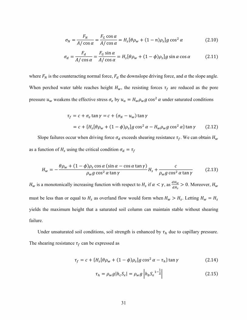
31
-G =àG
á/ cos k=àF cos ká/ cos k
= Ñ3[Kã6 + (1 − Z)ã3]ä cos* k(2.10)
-+ =à+
á/ cos k=àF sin ká/ cos k
= Ñ3[Kã6 + (1 − 5)ã3]ä sin k cos k (2.11)
where àG is the counteracting normal force, à+ the downslope driving force, and k the slope angle.
When perched water table reaches height Ñ6, the resisting forces W- are reduced as the pore
pressure Q6 weakens the effective stress -, by Q& = Ñ6ã6ä cos* k under saturated conditions
W- = & + -, tan P = & + (-G − Q6) tan P
= & + {Ñ3[Kã6 + (1 − 5)ã3]ä cos* k − Ñ6ã6ä cos* k} tan P (2.12)
Slope failures occur when driving force -+ exceeds shearing resistance W-.We can obtain Ñ6
as a function of Ñ3 using the critical condition -+ = W-
Ñ6 = −Kã6 + (1 − 5)ã3 cos k (sin k − cos k tan P)
ã6ä cos* k tan PÑ3 +
&ã6ä cos* k tan P
(2.13)
Ñ6 is a monotonically increasing function with respect to Ñ3 if k < P, as +H'+H(
> 0. Moreover, Ñ6
must be less than or equal to Ñ3 as overland flow would form whenÑ6 > Ñ3. Letting Ñ6 = Ñ3
yields the maximum height that a saturated soil column can maintain stable without shearing
failure.
Under unsaturated soil conditions, soil strength is enhanced by W: due to capillary pressure.
The shearing resistance W- can be expressed as
W- = & + {Ñ3[Kã6 + (1 − 5)ã3]ä cos* k − W:} tan P (2.14)
W: = ã6ä|ℎ"Ä,| = ã6ä éℎ1Ä,);)Ié (2.15)
32
with capillary pressure head ℎ", air-entry value ℎ1, pore size distribution parameter 1 (Brooks and
Corey, 1964), and effective saturation Ä,.
2.4 Results
2.4.1 Time-series Displacements and Annual Deformation Rates
From 2007 to 2011, sliding movement of the Lawson Creek landslide is captured by SAR data
from the ALOS ascending track T224. Figure 2.6a illustrates the time-series displacements of a
typical fast-moving point P (Figure 2.7c) between 2007 and 2011. As the measurement of one
single pixel can be easily contaminated by noises, we averaged the time-series deformation of the
3 × 3 array of adjacent points, which corresponds to a 60 m × 60 m area on the landslide surface.
Similarly, we mapped time-series displacements of the same point from 2016 to 2018 using
imagery from the Sentinel-1A/B ascending track T35, and from the ALOS-2 ascending track T68
for cross-validation. The results show that both the L-band ALOS-2 and the C-band Sentinel-1A/B
datasets produce highly similar results (Figure 2.6d). The cumulative downslope displacement of
the slide is about 1.5 m from 2007 to 2011 and around 0.8 m from 2016 to 2018, and movement
patterns resemble an annual cycle throughout the years: the sliding motion starts to accelerate after
wet seasons arrive and decelerates substantially when summer comes; while a considerable amount
of deformation occurs from mid-November to mid-May, few displacements appear during the dry
seasons from mid-May to mid-November (Figures 2.7d, 2.7e). Nevertheless, the landslide
movement does not totally stop even during dry summers; similar behaviors have been observed
at other landslides over the pacific northwest (Liu et al., 2013; Hu et al., 2018).
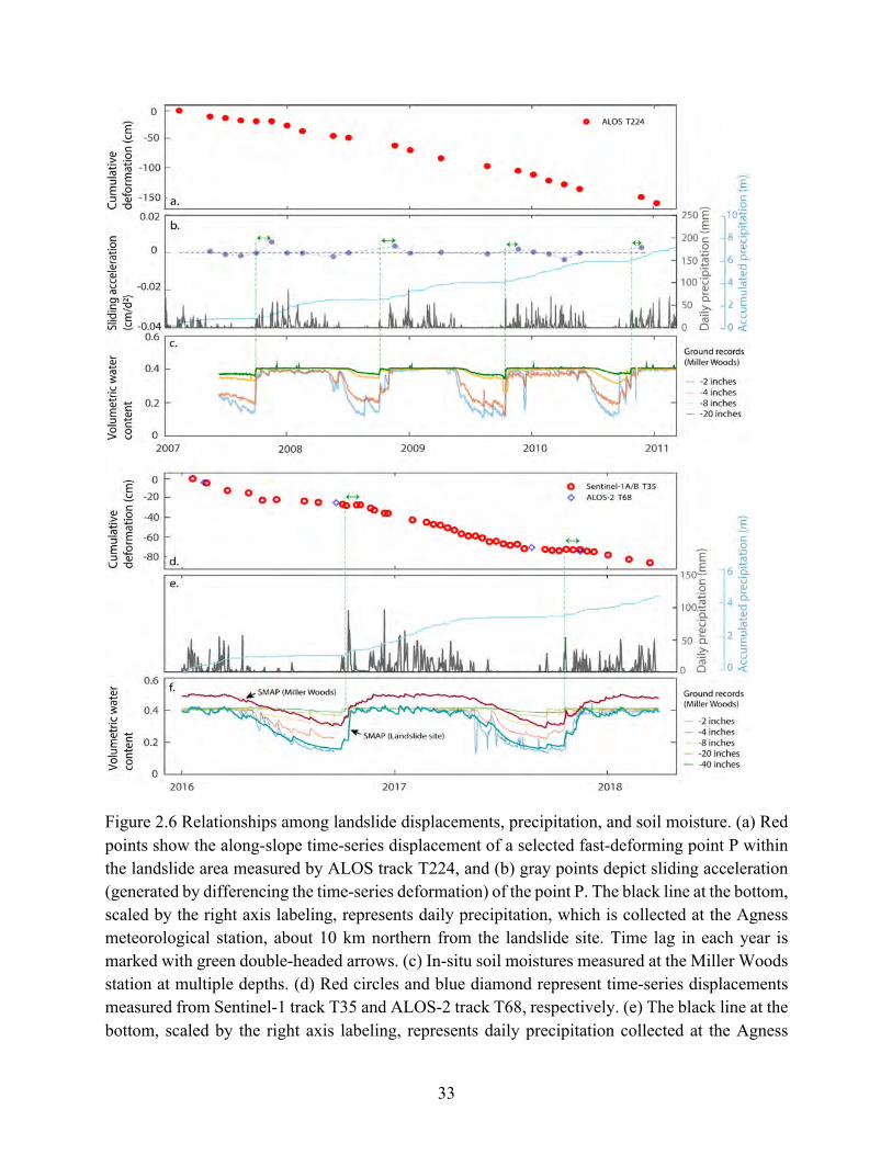
33
Figure 2.6 Relationships among landslide displacements, precipitation, and soil moisture. (a) Red points show the along-slope time-series displacement of a selected fast-deforming point P within the landslide area measured by ALOS track T224, and (b) gray points depict sliding acceleration (generated by differencing the time-series deformation) of the point P. The black line at the bottom, scaled by the right axis labeling, represents daily precipitation, which is collected at the Agness meteorological station, about 10 km northern from the landslide site. Time lag in each year is marked with green double-headed arrows. (c) In-situ soil moistures measured at the Miller Woods station at multiple depths. (d) Red circles and blue diamond represent time-series displacements measured from Sentinel-1 track T35 and ALOS-2 track T68, respectively. (e) The black line at the bottom, scaled by the right axis labeling, represents daily precipitation collected at the Agness
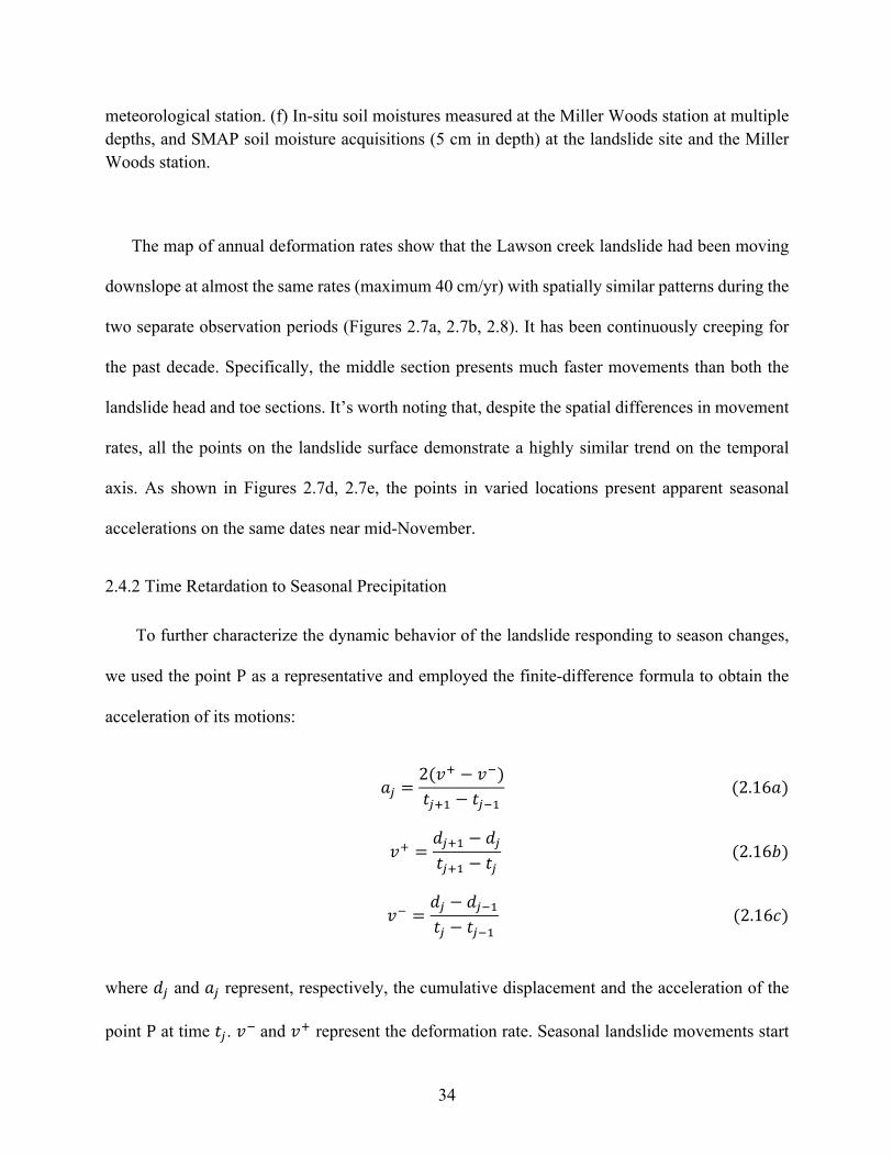
34
meteorological station. (f) In-situ soil moistures measured at the Miller Woods station at multiple depths, and SMAP soil moisture acquisitions (5 cm in depth) at the landslide site and the Miller Woods station.
The map of annual deformation rates show that the Lawson creek landslide had been moving
downslope at almost the same rates (maximum 40 cm/yr) with spatially similar patterns during the
two separate observation periods (Figures 2.7a, 2.7b, 2.8). It has been continuously creeping for
the past decade. Specifically, the middle section presents much faster movements than both the
landslide head and toe sections. It’s worth noting that, despite the spatial differences in movement
rates, all the points on the landslide surface demonstrate a highly similar trend on the temporal
axis. As shown in Figures 2.7d, 2.7e, the points in varied locations present apparent seasonal
accelerations on the same dates near mid-November.
2.4.2 Time Retardation to Seasonal Precipitation
To further characterize the dynamic behavior of the landslide responding to season changes,
we used the point P as a representative and employed the finite-difference formula to obtain the
acceleration of its motions:
Y9 =2(3J − 3;)X9J) − X9;)
(2.16Y)
3J =.9J) − .9X9J) − X9
(2.16ë)
3; =.9 − .9;)X9 − X9;)
(2.16&)
where .9 and Y9 represent, respectively, the cumulative displacement and the acceleration of the
point P at time X9. 3;and 3J represent the deformation rate. Seasonal landslide movements start
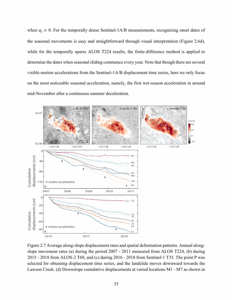
35
when Y9 > 0. For the temporally dense Sentinel-1A/B measurements, recognizing onset dates of
the seasonal movements is easy and straightforward through visual interpretation (Figure 2.6d),
while for the temporally sparse ALOS T224 results, the finite-difference method is applied to
determine the dates when seasonal sliding commence every year. Note that though there are several
visible motion accelerations from the Sentinel-1A/B displacement time series, here we only focus
on the most noticeable seasonal acceleration, namely, the first wet-season acceleration in around
mid-November after a continuous summer deceleration.
Figure 2.7 Average along-slope displacement rates and spatial deformation patterns. Annual along-slope movement rates (a) during the period 2007 - 2011 measured from ALOS T224, (b) during 2015 - 2018 from ALOS-2 T68, and (c) during 2016 - 2018 from Sentinel-1 T35. The point P was selected for obtaining displacement time series, and the landslide moves downward towards the Lawson Creek. (d) Downslope cumulative displacements at varied locations M1 - M7 as shown in
36
(a), mapped with ALOS T224 imagery. (e) Downslope cumulative displacements at varied locations S1 - S7 as shown in (c), mapped with Sentinel-1A/B T35 images.
Figure 2.8 Annual along-slope deformation rates of the landslide obtained from ALOS2 tracks T69 during 2014 - 2018 and T171 during 2015 - 2018.
As shown in Figures 2.6b, 2.6e, although the wet-season arrives in mid-October regularly
every year, the landslide does not begin to accelerate until several weeks later, generally in
November. However, the exact time lags vary by years. The maximum values stand at 41 days, 41
days, 31 days, 26 days, 43 days, and 37 days for 2007, 2008, 2009, 2010, 2016 and 2017
respectively (Figures 2.6a, 2.6d) as the displacements might happen before the date when satellites
capture the deformation. The 46-day revisit cycle of the ALOS acquisitions cannot provide an
effective lower bound to the time lags for years 2007 - 2011, but the Sentinel-1A/B datasets with
a minimum revisit period of six days successfully set the lower boundaries to 25 days for both
years 2016 and 2017. As the landslide always accelerate after the arrival of wet-seasons (i.e., the
37
theoretical lower boundary is 0 day), the time lag ranges are 0 - 41 days, 0 - 41 days, 0 - 31 days,
0 - 26 days, 25 - 43 days, and 25 - 37 days for 2007, 2008, 2009, 2010, 2016 and 2017, respectively.
Every year, the soil moisture gradually falls to a year low in the summer and rises back to a
high level as the wet-season approaches, and it maintains at this high level until the next summer
comes (Figures 2.6c, 2.6f). Here we define the arrival date of wet seasons as when the 40-inch-
depth (~ 1m) soil moisture at the Miller Woods station rises back to the same level of previous wet
seasons, based on the assumption that a few slight early-autumn rainfall events can hardly mark
the coming of wet seasons. In other words, the top 40-inch soils have been saturated.
There is a threefold justification for using soil moisture records from the Miller Woods station
to represent for the landslide site. First, both sites undergo almost the same rainfall events as
revealed by the SMAP soil moisture acquisitions at these two sites. As illustrated in Figure 2.6f,
each rise of the fluctuated SMAP soil moisture can be interpreted as a distinguishable rainfall
event, and SMAP data at both sites constantly exhibit such rise responses at the same dates. It’s
worth noting that SMAP soil moisture data used here are captured by satellites independently. The
values are the mean soil moisture of the top 5-centimeter soil layers, thus even slight rainfall events
can lead to a rising fluctuation on the SMAP data. Second, both sites have similar soil layer
compositions. Soils at the Miller woods station constitute layers of silt loam (0 - 16 cm depth),
silty clay loam (16 - 33 cm), silty clay (33 - 63 cm), and gravelly clay loam (63 - 152 cm). These
soil layers have similar saturated hydraulic conductivity as that at the landslide site, which
comprise of channery loam (0 - 30 cm), silt loam (30 - 56 cm), silty clay loam (56 - 74 cm), sandy
loam (74 - 158 cm), and silty clay loam (158 - 183 cm) (from NCSS soil pedons (USDA, 2019)
and local surveys (USDA, 1994)). Calculating infiltration time of the top 40-inch soils at both sites
using Equation (2.7) and the mean hydraulic conductivities in Table 2.2 shows that the landslide
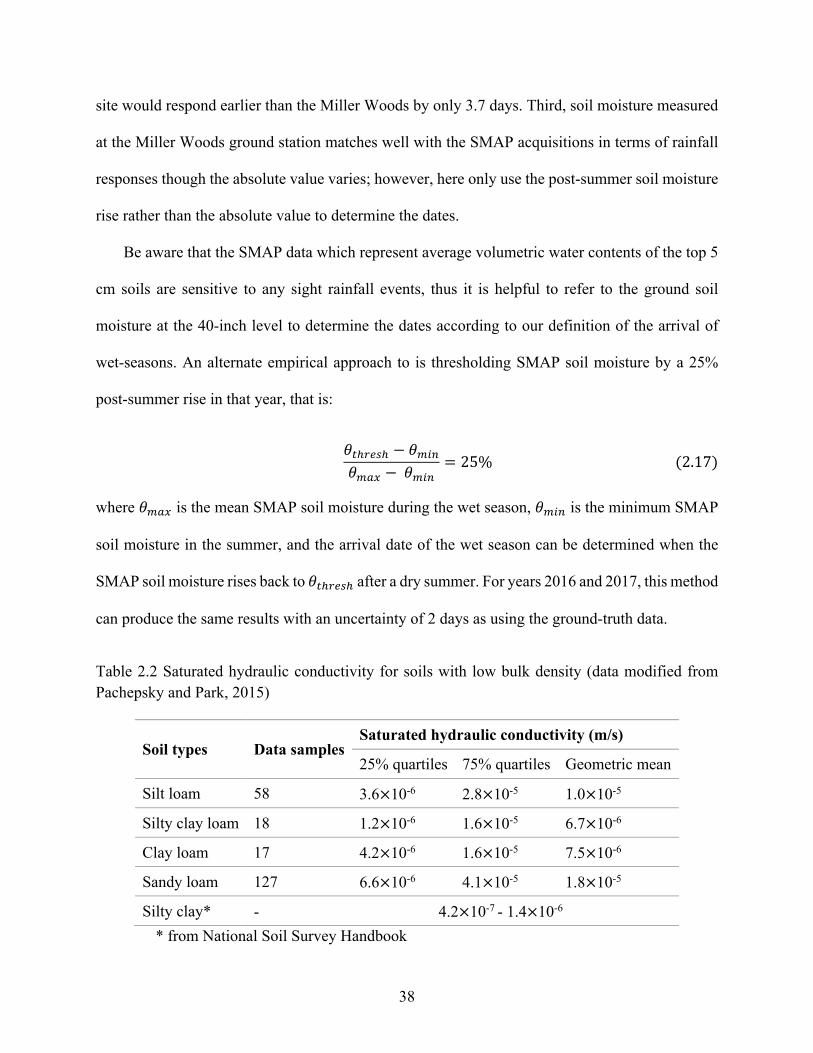
38
site would respond earlier than the Miller Woods by only 3.7 days. Third, soil moisture measured
at the Miller Woods ground station matches well with the SMAP acquisitions in terms of rainfall
responses though the absolute value varies; however, here only use the post-summer soil moisture
rise rather than the absolute value to determine the dates.
Be aware that the SMAP data which represent average volumetric water contents of the top 5
cm soils are sensitive to any sight rainfall events, thus it is helpful to refer to the ground soil
moisture at the 40-inch level to determine the dates according to our definition of the arrival of
wet-seasons. An alternate empirical approach to is thresholding SMAP soil moisture by a 25%
post-summer rise in that year, that is:
K%:#,3: − K0$2K0&= −K0$2
= 25%(2.17)
where K0&= is the mean SMAP soil moisture during the wet season, K0$2 is the minimum SMAP
soil moisture in the summer, and the arrival date of the wet season can be determined when the
SMAP soil moisture rises back to K%:#,3: after a dry summer. For years 2016 and 2017, this method
can produce the same results with an uncertainty of 2 days as using the ground-truth data.
Table 2.2 Saturated hydraulic conductivity for soils with low bulk density (data modified from Pachepsky and Park, 2015)
Soil types Data samples Saturated hydraulic conductivity (m/s)
25% quartiles 75% quartiles Geometric mean
Silt loam 58 3.6×10⁻⁶ 2.8×10⁻⁵ 1.0×10⁻⁵
Silty clay loam 18 1.2×10⁻⁶ 1.6×10⁻⁵ 6.7×10⁻⁶
Clay loam 17 4.2×10⁻⁶ 1.6×10⁻⁵ 7.5×10⁻⁶
Sandy loam 127 6.6×10⁻⁶ 4.1×10⁻⁵ 1.8×10⁻⁵
Silty clay* - 4.2×10⁻⁷ - 1.4×10⁻⁶
* from National Soil Survey Handbook
39
Soil moisture records at the 40-inch depth of the Miller Woods station are unavailable from
2007 to 2011, therefore, the corresponding time lags are calculated by using soil moisture data at
the 20-inch depth and adding on extra 5 days. The extra days are the observed time interval
between successive soil moisture surges at the 20-inch and 40-inch depths right after the 2016 and
2017 summers, which represent the water infiltration time from the 20-inch to the 40-inch depths
(Figure 2.6f).
2.4.2 Basal Depths and Volume Infered from InSAR Observations
Annual displacement rates from two ALOS-2 ascending tracks T68 and T69, one descending
track T171, and one Sentinel-1A/B ascending track T35 were employed to derive the 3D surface
velocity fields of the landslide (Table 2.1; Figures 2.7, 2.8). As the observations from the three
ascending tracks are not highly independent due to the similar LOS directions, we constrain the
landslide motions to be along-slope to achieve stable inversions. The 3D surface velocity vectors
are shown in Figures 2.9a, 2.9b.
Thickness inversion of surface points corresponding to every SAR-interferogram pixel (20 m
× 20 m) were implemented by using the mass conservation approach and assuming a power-law
rheology as Equation (2.1). Here the yield slope-perpendicular depth of each pixel has been
converted to vertical thickness (Figures 2.9c, 2.9d). The thickness map shows that the sliding plane
at the middle and upper sections are seated deepest, with a maximum mean basal depth of the
central region as 5.8 m to 7.8 m (Figure 2.9c, 2.9d), assuming the landslide is characterized by a
plug flow (2/3< ` < 1) as suggested by borehole measurements of multiple slow-moving
landslides (Delbridge et al., 2016; Wasowski, 1998; Gould, 1960; Mainsant et al., 2012; Iverson,
1985; Van Asch et al., 2009; Malet and Maquaire, 2003). The basal plane has an upwardly concave
shape that exhibits greater thickness in the central and gradually shallows to the margin area.
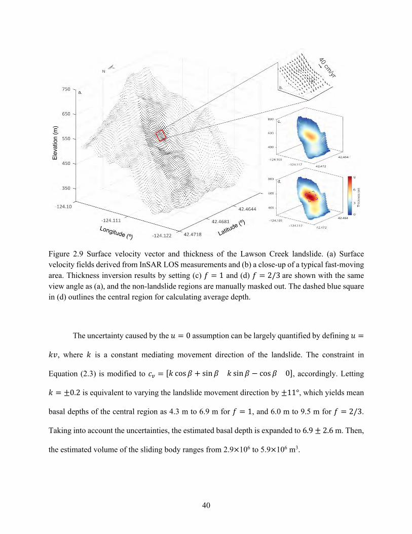
40
Figure 2.9 Surface velocity vector and thickness of the Lawson Creek landslide. (a) Surface velocity fields derived from InSAR LOS measurements and (b) a close-up of a typical fast-moving area. Thickness inversion results by setting (c) ` = 1 and (d) ` = 2/3are shown with the same view angle as (a), and the non-landslide regions are manually masked out. The dashed blue square in (d) outlines the central region for calculating average depth.
The uncertainty caused by the Q = 0 assumption can be largely quantified by defining Q =
x3, where x is a constant mediating movement direction of the landslide. The constraint in
Equation (2.3) is modified to &K = [x cos l + sin l x sin l − cos l 0], accordingly. Letting
x = ±0.2 is equivalent to varying the landslide movement direction by ±11°, which yields mean
basal depths of the central region as 4.3 m to 6.9 m for ` = 1, and 6.0 m to 9.5 m for ` = 2/3.
Taking into account the uncertainties, the estimated basal depth is expanded to 6.9 ± 2.6 m. Then,
the estimated volume of the sliding body ranges from 2.9×10⁶ to 5.9×10⁶ m3.
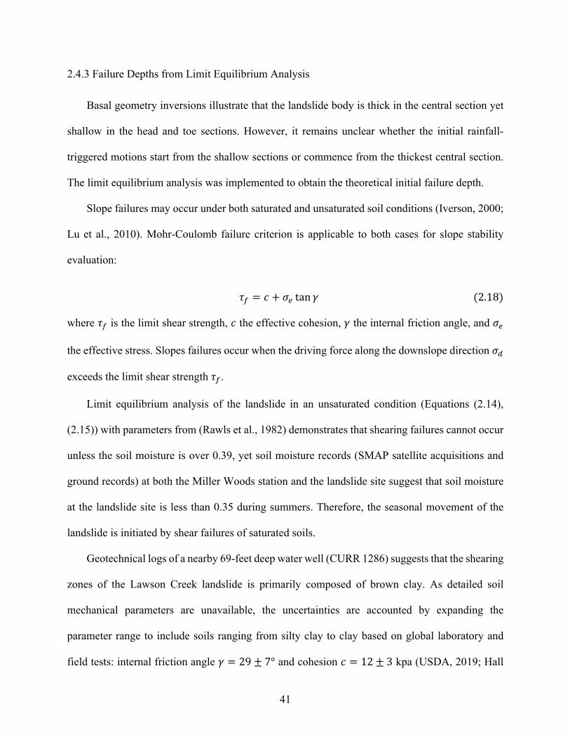
41
2.4.3 Failure Depths from Limit Equilibrium Analysis
Basal geometry inversions illustrate that the landslide body is thick in the central section yet
shallow in the head and toe sections. However, it remains unclear whether the initial rainfall-
triggered motions start from the shallow sections or commence from the thickest central section.
The limit equilibrium analysis was implemented to obtain the theoretical initial failure depth.
Slope failures may occur under both saturated and unsaturated soil conditions (Iverson, 2000;
Lu et al., 2010). Mohr-Coulomb failure criterion is applicable to both cases for slope stability
evaluation:
W- = & + -, tan P (2.18)
where W- is the limit shear strength, & the effective cohesion, P the internal friction angle, and -,
the effective stress. Slopes failures occur when the driving force along the downslope direction -+
exceeds the limit shear strength W-.
Limit equilibrium analysis of the landslide in an unsaturated condition (Equations (2.14),
(2.15)) with parameters from (Rawls et al., 1982) demonstrates that shearing failures cannot occur
unless the soil moisture is over 0.39, yet soil moisture records (SMAP satellite acquisitions and
ground records) at both the Miller Woods station and the landslide site suggest that soil moisture
at the landslide site is less than 0.35 during summers. Therefore, the seasonal movement of the
landslide is initiated by shear failures of saturated soils.
Geotechnical logs of a nearby 69-feet deep water well (CURR 1286) suggests that the shearing
zones of the Lawson Creek landslide is primarily composed of brown clay. As detailed soil
mechanical parameters are unavailable, the uncertainties are accounted by expanding the
parameter range to include soils ranging from silty clay to clay based on global laboratory and
field tests: internal friction angle P = 29 ± 7° and cohesion & = 12 ± 3 kpa (USDA, 2019; Hall
42
et al., 1994; Alto, 1981; MnDOT, 2019; Ouyang and Mayne, 2017; Jeong et al., 2017; Thunder
2016; Msilimba, 2007). The slope angles of the landslide on the basal surface is less than 15°.
Using the measured volumetric water content K = 0.41 during wet-seasons and soil porosity 5 =
0.47 (Rawls, 1982), we can obtain the critical basal depth Ñ" = 7.6 ± 1.6m where shearing
failures would commence using Equation (2.13), based on the Mohr-Coulomb failure criterion.
This result agrees well with the InSAR-inferred basal depth of 6.9 ± 2.6 m, which confirms the
correctness of the inverted thickness based on mass conservation and surface velocities.
Meanwhile, it indicates that the deep-seated central region is close to stress equilibrium when the
soils are fully saturated, and a slight pore pressure rise would trigger the motion acceleration. Note
that the landslide had motions even during the dry summer, while intermittent post-summer rainfall
did not cause simultaneous motion acceleration (Figure 2.6), implying that the seasonal
acceleration is caused by pore pressure rise rather than loading from rainwater.
2.4.4 Potential for Estimating Hydraulic Parameters
Taking into account the uncertainties caused by SMAP data (±2days) and soil compositions
(-3.7 days), the time lags of 25 - 43 days observed from satellite remote sensing is expanded to
26.7 - 48.7 days. With the known time lags and InSAR-inferred basal depth of 6.9 ± 2.6m, the
rainwater infiltration rate can be quantified. Here the time lags stand for water infiltration from the
40-inch depth to the initial failure depth.
As groundwater level decreases during the dry summers, initial wet-season precipitation must
saturate the top soil layers via advective flow first before the hydraulic diffusion process takes
control of the basal pore-pressure response. The averaged hydraulic conductivity of soil layers
above the groundwater table and the averaged hydraulic diffusivity below the table can both be
effectively quantified with given groundwater levels. However, such data is not available for this
43
case study and therefore only the upper and lower bound of the hydraulic parameters can be
estimated.
Assuming the groundwater table is below the basal plane leads to an estimate of characteristic
hydraulic conductivity �3 (upper bound) as 2.4×10⁻⁵ m/s using Equations (2.5), (2.7), whereas
assuming fully saturated soils yields an estimated characteristic hydraulic diffusivity Ü!(lower
bound) as 2.6×10⁻⁶ m2/s using Equation (2.8). Note that here characteristic hydraulic
conductivity/diffusivity means to treat a soil column that constitutes multiple heterogeneous layers
as one single soil sample.
Employing empirical relationship between �3 and Ü! of the same soils can provide the other
bounds for the estimations. The vertical soil profile of the Lawson Creek landslide comprises
boulders and clay brown, clay brown, and clay blue layers from the nearby water well log (CURR
1286), we interpret the characteristic hydraulic conductivity as similar to that of silty clay and
obtain an empirical approximation as Ü! = 10* ⋅ �3 (Lambe and Whitman, 2008; Berti and
Simoni, 2010). It can yield a lower bound for the �3 as 2.6×10⁻⁸ m/s and an upper bound for Ü!
as 3.7×10⁻⁴ m2/s. Accordingly, combining both approaches can bound the characteristic hydraulic
conductivity to (2.6×10⁻⁸, 2.4×10⁻⁵) m/s and the characteristic hydraulic diffusivity to (2.6×10⁻⁶,
3.7×10⁻⁴) m2/s. The average is given as �3=1.2×10⁻⁵ m/s and Ü!=1.9×10⁻⁴ m2/s. Given the fact
that even field-measured hydraulic conductivity has an uncertainty by three orders (Berti and
Simoni,2010; Berti and Simoni, 2012), the above-described estimations is of important practical
value.
2.5 Discussion
In this investigation, basal depth inversion of the landslide is achieved based on mass
conservation and InSAR-captured surface velocity. A Q = 0 (Figure 2.5) assumption is employed
44
to reconstruct the 3D surface velocity field as currently spaceborne SAR images can only provide
two independent LOS observations. This assumption largely agrees with the landslide behavior
monitored by continuous GPS (Global Positioning System) at several sites (Hu et al., 2018;
Madson et al., 2019) and can provide a reasonable estimation of the thickness distribution over the
whole landslide area, as confirmed by the uncertainty analysis and by the independent limit
equilibrium analysis by feeding a wide range of soil mechanical parameters. Besides, it is worth
noting that the selected wide range of rheological parameter (2/3 < ` < 1) has also partly
compensated the uncertainty derived from 3D surface velocity reconstruction.
Determining the starting date of the wet season is a key difficulty in estimating time lags.
Thresholding cumulative precipitation is one of the options. However, analyzing cumulative
rainfall from summer to the date of the first motion acceleration reveals that there are significant
variations by years. For instance, the cumulative precipitation stands at 290 mm, 256 mm, 232
mm, 341 mm, 381 mm, and 336 mm for year 2007, 2008, 2009, 2010, 2016 and 2017, respectively
(Figure 2.6b, 2.6e), which can hardly lead to a reliable and accurate threshold value. In-situ
precipitation data show that the first several post-summer rainfall events are generally intermittent,
while a single rainfall event cannot represent the arrival of wet-seasons. Cumulative rainfall
infiltrates into the basal plane to trigger seasonal landslide motions, yet a single rainfall with a
short duration and a small intensity is unlikely to saturate the entire sliding material and raise pore
pressure on the basal plane. In contrast, the soil moisture that reflects the degree of saturation of
soils can thus be a good indicator to define the starting date of wet seasons.
The lack of in-situ measurements such as groundwater level from this faraway landslide site
has posed challenges to the hydraulic parameter estimation. Hence, only lower and upper bounds
for characteristic hydraulic conductivity and diffusivity are estimated. To account for all related
45
uncertainties, the average basal depth of the central landslide region is used, rather than a single
point. The derived time lags also have included the uncertainties that stem from satellite revisit
cycle and varied soil moisture methods and locations. Due to the limited field data, here we only
aim to layout a framework for estimating landslide thickness and corresponding hydraulic
parameters, and better results can be obtained if more field data are available.
Regarding SAR datasets for landslide studies, L-band data overall exhibit better coherence on
vegetated terrain than C-band data, while the C-band sentinel-1 imagery has unique advantages on
time-series mapping due to the dense temporal acquisitions. The free ALOS and Sentinel-1 images
have greatly contributed the data availability between 2007 and 2011 and after 2015, and the gap
between 2011 and 2015 can be filled with commercial SAR datasets. Currently, spaceborne SAR
datasets can only provide two independent observations, yet incorporating data from airborne
missions such as Uninhabited Aerial Vehicle SAR (UAVSAR (Rosen et al., 2006)) is a potential
solution to obtain real three-dimensional surface velocity fields of a landslide.
The Lawson Creek landslide is a typical slow-moving slide that is seated on the deposit of an
ancient landslide (> 150 years (Burns, 2014)). The slow-moving behavior is very likely attributed
to the soil porosity (Iverson et al. 2000) yet the seasonal dynamics are primarily associated with
precipitation. InSAR observations reveal that the central region has greater displacement rate than
the toe and head sections, which potentially implies that the central area is the active part, while
movements of the landslide head and toe might be passive. During the past decade, the moving
rate has been slow and stable, and currently no signs of runout have been captured.
2.6 Conclusions
This investigation employs multiple SAR datasets including ALOS, ALOS-2, and Sentinel
images spanning 2007-2011 and 2016-2018 to map time-series displacement of a translational
46
landslide in the southern Oregon, which reveals that the landslide has been continuously creeping
for the whole past decade with a maximum rate of 40 cm/yr in the upper middle section. The
landslide motion exhibits apparent seasonal patterns with considerable displacements during wet
seasons from mid-November to mid-May while little deformation during dry summers. The basal
depth of the landslide is inverted based on mass conservation theory and InSAR-inferred surface
velocity fields by assuming a power-law rheology. The results show that the Lawson Creek
landslide is seated deepest in the central region and gradually shallow to the margin area. The
mean thickness of the central region stands at 6.9 ± 2.6 meters. This estimation is also validated
and confirmed by an independent limit equilibrium analysis which demonstrates that initial
shearing failure of saturated soil columns would occur at 7.6 ± 1.6m depth.
The time lags between the arrival of wet seasons and the onset of seasonal landslide
motions are determined based on the observed periodic post-summer rise of soil moisture (SMAP
and ground records) and InSAR time-series measurements. During the observation period, the time
lags range from 26.7 to 48.7 days including uncertainties. InSAR observations reveals that the
landslide kept moving even during dry summers and intermittent post-summer rainfall did not
cause simultaneous acceleration of landslide motion, implying that seasonal accelerations are
caused by basal pore-pressure rise rather than loading of rainwater. Accordingly, we take the water
infiltration as purely advective flow and purely water diffusion respectively to estimate the lower
and upper bounds of the characteristic hydraulic conductivity �3 and diffusivity Ü! of the landslide
material, as groundwater level data are unavailable. The yield average values are �3=1.2×10⁻⁵ m/s
and Ü!=1.9×10⁻⁴ m2/s.
As with most landslides all over the globe, for the Lawson Creek landslide, in-situ
measurements of basal depth and hydraulic parameters are unavailable despite their importance

47
for characterizing landslide behaviors. However, here we have explored the possibility of using
primarily remote sensing datasets to infer the landslide thickness and estimate the hydraulic
conductivity and diffusivity. More importantly, this established framework is able to yield better
estimates when extra inputs are available. For instance, thickness inversion can be improved with
more than there independent LOS observations, and hydraulic estimations can be enhanced with
known groundwater levels.

48
ACKNOWLEDGEMENTS
This research was financially supported by NASA Interdisciplinary Research (IDS) in Earth
Science Program (80NSSC17K0022) and the Shuler-Foscue Endowment at Southern Methodist
University. Precipitation data were obtained from Western Regional Climate Center (WRCC)
(https://wrcc.dri.edu/). Ground soil moisture data were accessed from Natural Resources
Conservation Services (NRCS, SNOTEL products) (https://www.wcc.nrcs.usda.gov/). ALOS
PALSAR datasets were copyrighted by the Japan Aerospace Exploration Agency (JAXA) and
provided by Alaska Satellite Facility (ASF). Sentinel-1A/B collections were copyrighted by the
European Space Agency (ESA) and provided by ASF. ALOS PALSAR-2 data were provided by
Dr. Jinwoo Kim under JAXA ALOS-2 proposal (PI No. 3116). SMAP soil moisture data were
provided by the National Aeronautics and Space Administration (NASA).
49
REFERENCES
Alto, J. V. (1981). Engineering properties of Oregon and Washington coast range soils.
Aryal, A., Brooks, B. A., and Reid, M. E. (2015). Landslide subsurface slip geometry inferred from 3‐D surface displacement fields. Geophysical Research Letters, 42(5), 1411-1417.
Baum, R. L., and Reid, M. E. (1995). Geology, hydrology, and mechanics of a slow-moving, clay-rich landslide, Honolulu, Hawaii. Clay Shale Slope Instability, 10, 79.
Berardino, P., Fornaro, G., Lanari, R., and Sansosti, E. (2002). A new algorithm for surface deformation monitoring based on small baseline differential SAR interferograms. IEEE Transactions on geoscience and remote sensing, 40(11), 2375-2383.
Berti, M., and Simoni, A. (2010). Field evidence of pore pressure diffusion in clayey soils prone to landsliding. Journal of Geophysical Research: Earth Surface, 115(F3).
Berti, M., and Simoni, A. (2012). Observation and analysis of near‐surface pore‐pressure measurements in clay‐shales slopes. Hydrological Processes, 26(14), 2187-2205.
Bogaard, T. A., and Greco, R. (2016). Landslide hydrology: from hydrology to pore pressure. Wiley Interdisciplinary Reviews: Water, 3(3), 439-459.
Booth, A. M., Lamb, M. P., Avouac, J. P., and Delacourt, C. (2013). Landslide velocity, thickness, and rheology from remote sensing: La Clapière landslide, France. Geophysical Research Letters, 40(16), 4299-4304.
Brooks, R. H., and Corey, A. T. (1964). Hydraulic properties of porous media (Doctoral dissertation, Colorado State University. Libraries).
Burns, W. J. (2014) Statewide landslide information database for Oregon [SLIDO], release 3.2: Oregon Department of Geology and Mineral Industries, geodatabase. Web: http://www.oregongeology.org/sub/slido
Cascini, L., Fornaro, G., and Peduto, D. (2010). Advanced low-and full-resolution DInSAR map generation for slow-moving landslide analysis at different scales. Engineering Geology, 112(1-4), 29-42.
Delbridge, B. G., Bürgmann, R., Fielding, E., Hensley, S., and Schulz, W. H. (2016). Three‐dimensional surface deformation derived from airborne interferometric UAVSAR:
50
Application to the Slumgullion Landslide. Journal of geophysical research: solid earth, 121(5), 3951-3977.
Gould, J. P. (1960). A study of shear failure in certain Tertiary marine sediments. In Research Conference on Shear Strength of Cohesive Soils, Boulder, Colorado, 1960 (pp. 615-641).
Grant, M., and Boyd, S. (2014). CVX: Matlab software for disciplined convex programming, version 2.1.
Prellwitz, R. W. (1994). Slope stability reference guide for National Forests in the United States (Vol. 1). US Department of Agriculture, Forest Service, Engineering Staff.
Hilley, G. E., Bürgmann, R., Ferretti, A., Novali, F., and Rocca, F. (2004). Dynamics of slow-moving landslides from permanent scatterer analysis. Science, 304(5679), 1952-1955.
Hu, X., Lu, Z., Pierson, T. C., Kramer, R., and George, D. L. (2018). Combining InSAR and GPS to determine transient movement and thickness of a seasonally active low‐gradient translational landslide. Geophysical Research Letters, 45(3), 1453-1462.
Iverson, R. M. (1985). A constitutive equation for mass-movement behavior. The Journal of Geology, 93(2), 143-160.
Iverson, R. M. (2000). Landslide triggering by rain infiltration. Water resources research, 36(7), 1897-1910.
Iverson, R. M., George, D. L., Allstadt, K., Reid, M. E., Collins, B. D., Vallance, J. W., Schilling, S. P., Godt, J. W., Cannon, C. M., Magirl, C. S. and Baum, R. L. (2015). Landslide mobility and hazards: implications of the 2014 Oso disaster. Earth and Planetary Science Letters, 412, 197-208.
Iverson, R. M., and Major, J. J. (1987). Rainfall, ground-water flow, and seasonal movement at Minor Creek landslide, northwestern California: Physical interpretation of empirical relations. Geological Society of America Bulletin, 99(4), 579-594.
Iverson, R. M., Reid, M. E., Iverson, N. R., LaHusen, R. G., Logan, M., Mann, J. E., and Brien, D. L. (2000). Acute sensitivity of landslide rates to initial soil porosity. science, 290(5491), 513-516.
Jebur, M. N., Pradhan, B., and Tehrany, M. S. (2014). Detection of vertical slope movement in highly vegetated tropical area of Gunung pass landslide, Malaysia, using L-band InSAR technique. Geosciences Journal, 18(1), 61-68.
Jeong, S., Lee, K., Kim, J., and Kim, Y. (2017). Analysis of rainfall-induced landslide on unsaturated soil slopes. Sustainability, 9(7), 1280.
Lambe, T. W., and Whitman, R. V. (2008) Soil mechanics SI version. John Wiley and Sons.
51
Lehmann, P., and Or, D. (2012). Hydromechanical triggering of landslides: From progressive local failures to mass release. Water Resources Research, 48(3).
Liu, P., Li, Z., Hoey, T., Kincal, C., Zhang, J., Zeng, Q., and Muller, J. P. (2013). Using advanced InSAR time series techniques to monitor landslide movements in Badong of the Three Gorges region, China. International Journal of Applied Earth Observation and Geoinformation, 21, 253-264.
Lu, N., Godt, J. W., and Wu, D. T. (2010). A closed‐form equation for effective stress in unsaturated soil. Water Resources Research, 46(5).
Madson, A., Fielding, E., Sheng, Y., and Cavanaugh, K. (2019). High-resolution spaceborne, airborne and in situ landslide kinematic measurements of the slumgullion landslide in Southwest Colorado. Remote Sensing, 11(3), 265.
Mainsant, G., Larose, E., Brönnimann, C., Jongmans, D., Michoud, C., and Jaboyedoff, M. (2012). Ambient seismic noise monitoring of a clay landslide: Toward failure prediction. Journal of Geophysical Research: Earth Surface, 117(F1).
Malet, J. P., and Maquaire, O. (2003, May). Black marl earthflows mobility and long-term seasonal dynamic in southeastern France. In Proc. 1st Int. Conf. on Fast Slope Movements (pp. 333-340).
MnDOT (Minnesota Department of Transportation) (2007) MnDOT Pavement Design Manual. http://www.dot.state.mn.us/materials/pvmtdesign/docs/2007manual/Chapter_3-2.pdf
Msilimba, G. G. A. C. (2007). A comparative study of landslides and geohazard mitigation in northern and central Malawi (Doctoral dissertation, University of the Free State).
Mualem, Y. (1976). A new model for predicting the hydraulic conductivity of unsaturated porous media. Water resources research, 12(3), 513-522.
Nikolaeva, E., Walter, T. R., Shirzaei, M., and Zschau, J. (2014). Landslide observation and volume estimation in central Georgia based on L-band InSAR. Natural Hazards and Earth System Sciences, 14(3), 675-688.
Ouyang, Z., and Mayne, P. W. (2018). Effective friction angle of clays and silts from piezocone penetration tests. Canadian Geotechnical Journal, 55(9), 1230-1247.
Pachepsky, Y., and Park, Y. (2015). Saturated hydraulic conductivity of US soils grouped according to textural class and bulk density. Soil Science Society of America Journal, 79(4), 1094-1100.
Priest, G. R., Schulz, W. H., Ellis, W. L., Allan, J. A., Niem, A. R., and Niem, W. A. (2011). Landslide stability: role of rainfall-induced, laterally propagating, pore-pressure waves. Environmental and Engineering Geoscience, 17(4), 315-335.
52
Rawls, W. J., Brakensiek, D. L., and Saxtonn, K. E. (1982). Estimation of soil water properties. Transactions of the ASAE, 25(5), 1316-1320.
Reid, M. E. (1994). A pore-pressure diffusion model for estimating landslide-inducing rainfall. The Journal of Geology, 102(6), 709-717.
Rosen, P.A., Hensley, S., Wheeler, K., Sadowy, G., Miller, T., Shaffer, S., Muellerschoen, R., Jones, C., Zebker, H. and Madsen, S. (2006, April). UAVSAR: A new NASA airborne SAR system for science and technology research. In 2006 IEEE Conference on Radar (pp. 8-pp). IEEE.
Rutt, I. C., Hagdorn, M., Hulton, N. R. J., and Payne, A. J. (2009). The Glimmer community ice sheet model. Journal of Geophysical Research: Earth Surface, 114(F2).
Schlögel, R., Doubre, C., Malet, J. P., and Masson, F. (2015). Landslide deformation monitoring with ALOS/PALSAR imagery: A D-InSAR geomorphological interpretation method. Geomorphology, 231, 314-330.
Thunder, B. (2016). Hydro-mechanical analysis of an infiltration-induced landslide along I-70 in Summit County, CO, The (Doctoral dissertation, Colorado School of Mines).
Tong, X., and Schmidt, D. (2016). Active movement of the Cascade landslide complex in Washington from a coherence-based InSAR time series method. Remote Sensing of Environment, 186, 405-415.
USDA (2019) National cooperative soil survey soil characterization data. https://ncsslabdatamart.sc.egov.usda.gov
USDA (1994) Soil Survey of Curry County, Oregon. https://www.nrcs.usda.gov/Internet/FSE_MANUSCRIPTS/oregon/OR015/0/Curry.pdf
Van Asch, T. W., Malet, J. P., and Bogaard, T. A. (2009). The effect of groundwater fluctuations on the velocity pattern of slow-moving landslides. Natural Hazards and Earth System Sciences, 9(3), 739-749.
Van Genuchten, M. T. (1980). A closed‐form equation for predicting the hydraulic conductivity of unsaturated soils. Soil science society of America journal, 44(5), 892-898.
Wartman, J., Montgomery, D. R., Anderson, S. A., Keaton, J. R., Benoît, J., dela Chapelle, J., and Gilbert, R. (2016). The 22 March 2014 Oso landslide, Washington, USA. Geomorphology, 253, 275-288.
Wasowski, J. (1998). Inclinometer and piezometer record of the 1995 reactivation of the Acquara-Vadoncello landslide, Italy. In Engineering Geology: A global view from the Pacific Rim (pp. 1697-1704).

53
Werner, C., Wegmüller, U., Strozzi, T., and Wiesmann, A. (2000, October). Gamma SAR and interferometric processing software. In Proceedings of the ers-envisat symposium, Gothenburg, Sweden (Vol. 1620, p. 1620).
Xu, Y., Kim, J., George, D. L., and Lu, Z. (2019). Characterizing seasonally rainfall-driven movement of a translational landslide using SAR imagery and SMAP soil moisture. Remote Sensing, 11(20), 2347.
54
CHAPTER 3
DYNAMICS AND PHYSICS-BASED RAINFALL THRESHOLDS FOR THE
DEEP-SEATED HOOSKANADEN LANDSLIDE, OREGON
Xu, Y., Lu, Z., Schulz, W. H., and Kim, J. (2020). Twelve‐Year Dynamics and Rainfall Thresholds for Alternating Creep and Rapid Movement of the Hooskanaden Landslide from Integrating InSAR, Pixel Offset Tracking, and Borehole and Hydrological Measurements. Journal of Geophysical Research: Earth Surface, 125(10), e2020JF005640.
3.1 Introduction
Landslides annually cause billions of dollars of property loss and thousands of casualties on a
global scale (Spiker and Gori, 2003; Froude and Petley, 2018), and act as a primary instrument for
geomorphic changes in many regions (Mackey and Roering, 2011; Simoni et al., 2013). Mitigating
landslide hazards and understanding landslide-induced landscape evolution require knowledge of
landslide kinematics and timing. However, the timing of deep-seated landslides is particularly
problematic to forecast even with subsurface pore-water pressure observations (Angeli et al., 1996;
Massey et al., 2013; Gasparitto et al., 1996; Schulz et al., 2009, 2018; Pyles et al., 1987). Here we
sought to use multiple remote sensing approaches and ground precipitation records to characterize
motion behaviors of a typical deep-seated coastal landslide, and to develop a rainfall thresholding
strategy for forecasting the timing of its movements.
55
The Hooskanaden landslide, located in southwestern Oregon and crossed by U.S. Highway
101, has been constantly damaging the highway and has resulted in significant repair costs to the
Oregon Department of Transportation (ODOT). The slide is large (~600 m wide × 1,300 m long),
deep (~30-45m), and has been active since at least 1958 (Parker, 1979) with typically slow motions
in most years and occasional destructive moderate to major movements. Road maintenance during
the slow-moving years annually cost ODOT about $75,000, while repair costs of a single major
event usually amount to $5-7 million (ODOT, 2019). The most recent major event occurred on
February 25, 2019, which displaced the road surface about 40 meters to the west and 17 meters
downward (Figure 3.1; Britton, 2019) and closed the highway for 13 days until a temporary gravel
lane was opened (ODOT, 2019). Two paved lanes were later reconstructed and opened on May 6,
and a total of $1.12 million had been spent by that time (ODOT, 2019). The Hooskanaden slide is
a distinct example demonstrating that deep-seated landslides with long-term creeping behaviors
may also move violently at certain times and cause significant damages.
To understand the motion behaviors of the Hooskanaden landslide, multiple remote sensing
datasets and tools, borehole measurements, and hydrological observations were used for this
investigation to retrieve its long-term surface and subsurface displacement history and reveal the
role that precipitation plays. Specifically, InSAR (Interferometric Synthetic Aperture Radar) and
pixel offset tracking of SAR images, optical images, and LiDAR (Light Detection and Ranging)
DEMs (Digital Elevation Model) were implemented to quantify the time-series motion of the
landslide from 2007 to 2019. The 2019 February event with significant block-like movements
provided a special opportunity to reconstruct the three-dimensional surface deformation field by
using pixel offset tracking of both the Sentinel-1 SAR images and the Sentinel-2 optical images.
In addition, borehole inclinometer measurements were employed to reveal the landslide’s
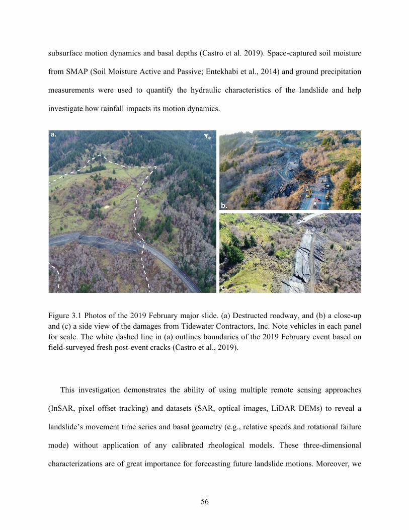
56
subsurface motion dynamics and basal depths (Castro et al. 2019). Space-captured soil moisture
from SMAP (Soil Moisture Active and Passive; Entekhabi et al., 2014) and ground precipitation
measurements were used to quantify the hydraulic characteristics of the landslide and help
investigate how rainfall impacts its motion dynamics.
Figure 3.1 Photos of the 2019 February major slide. (a) Destructed roadway, and (b) a close-up and (c) a side view of the damages from Tidewater Contractors, Inc. Note vehicles in each panel for scale. The white dashed line in (a) outlines boundaries of the 2019 February event based on field-surveyed fresh post-event cracks (Castro et al., 2019).
This investigation demonstrates the ability of using multiple remote sensing approaches
(InSAR, pixel offset tracking) and datasets (SAR, optical images, LiDAR DEMs) to reveal a
landslide’s movement time series and basal geometry (e.g., relative speeds and rotational failure
mode) without application of any calibrated rheological models. These three-dimensional
characterizations are of great importance for forecasting future landslide motions. Moreover, we
57
successfully developed a threefold hydrological threshold to forecast the timing of the deep-seated
landslide’s seasonal onsets and moderate/major movements, by integrating shallow soil moisture
from SMAP and daily/hourly ground precipitation. In contrast to the demanding and sometimes
unreliable pore-pressure thresholds (Angeli et al., 1996; Massey et al., 2013; Gasparitto et al.,
1996), our hydrological thresholds do not require any expensive, potentially dangerous or
impossible subsurface exploration and monitoring of pore-water pressures, and therefore can be
easily adapted for other similar landslides.
3.2 Geological Setting and Historical Activities
3.2.1 Geographical and Geological Settings
The Hooskanaden landslide is located in Curry County, Oregon (Figure 3.2). It is crossed near
its center by U.S. Highway 101, and its toe reaches the Pacific Ocean (Figure 3.2b). The landslide
crown is located at about 200 m in elevation, and the currently active body is about 1,300 m long
and 600 m wide, with an average slope of 17 . Moderate surface vegetation consisting of grasses
and deciduous and coniferous trees covers the lower half of the slide below the road, while sparse
vegetation grows on the upper half (Figure 3.1a). The regional topography from the hillshade map
(Figure 3.2b) indicates that the landslide at Hooskanaden may have experienced a large ancient
event, along with subsequent fluvial erosions and mass wasting that have significantly modified
the original landforms.
Materials of the slide are derived from the Otter Point Formation of late Jurassic geologic age
(Walker and Macleod, 1991), which consists of a matrix of sheared sandstone, mudstone,
conglomerate, and interbedded sandstone and shale, with scattered BIMs (blocks-in-matrix,
composed of more resistant sandstone, greenstones, chert and blueschist). These materials,
geologically referred to as mélange (Castro et al., 2019), were accumulated as an accretionary
58
wedge along the Cascadia subduction zone during tectonic displacement and formed the accreted
western margin of the Klamath Mountains region (Orr and Orr, 2012). Stratigraphically, the slide
consists of harder upper layers with predominantly sandstone and softer lower layers of mixed
shale and siltstone, as indicated by samples collected from four boreholes drilled between
September 1978 and January 1979 (Boreholes 1-4 in Figure 3.2a; Parker, 1979) and one borehole
drilled in December 2017 (BH-5 in Figure 3.2a, ODOT drilling logs [Hole No. SPR808-H1]).
Rocks in the borehole are either moderately weathered or highly fractured with numerous joints
and slickensides. Depths of the main mass vary from 30 to 45 meters (Parker, 1979).
Surface deformation patterns including localized slumps, compression ridges, transverse/semi-
transverse internal cracks and closed depressions (Figure 3.2b) indicate that the whole landslide
comprises several compartmentalized zones of movement rather than a single mass moving as a
coherent block. Individual compartment masses partly move along discrete basal shear zones but
together contribute to the overall movement of the slide mass by alternatively providing and
removing passive resistance and/or driving force to the compartments above and below. Lateral
slide boundaries are potentially constrained by large BIMs present along the flanks of the landslide
(Castro et al. 2019).
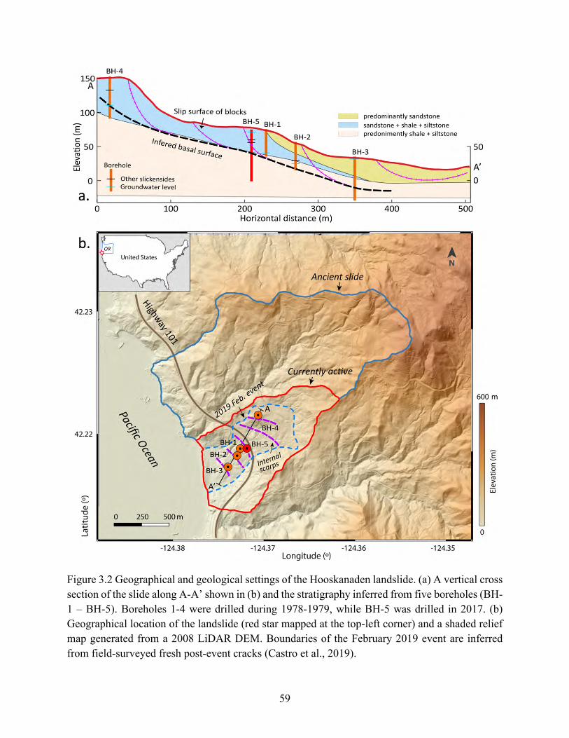
59
Figure 3.2 Geographical and geological settings of the Hooskanaden landslide. (a) A vertical cross section of the slide along A-A’ shown in (b) and the stratigraphy inferred from five boreholes (BH-1 – BH-5). Boreholes 1-4 were drilled during 1978-1979, while BH-5 was drilled in 2017. (b) Geographical location of the landslide (red star mapped at the top-left corner) and a shaded relief map generated from a 2008 LiDAR DEM. Boundaries of the February 2019 event are inferred from field-surveyed fresh post-event cracks (Castro et al., 2019).
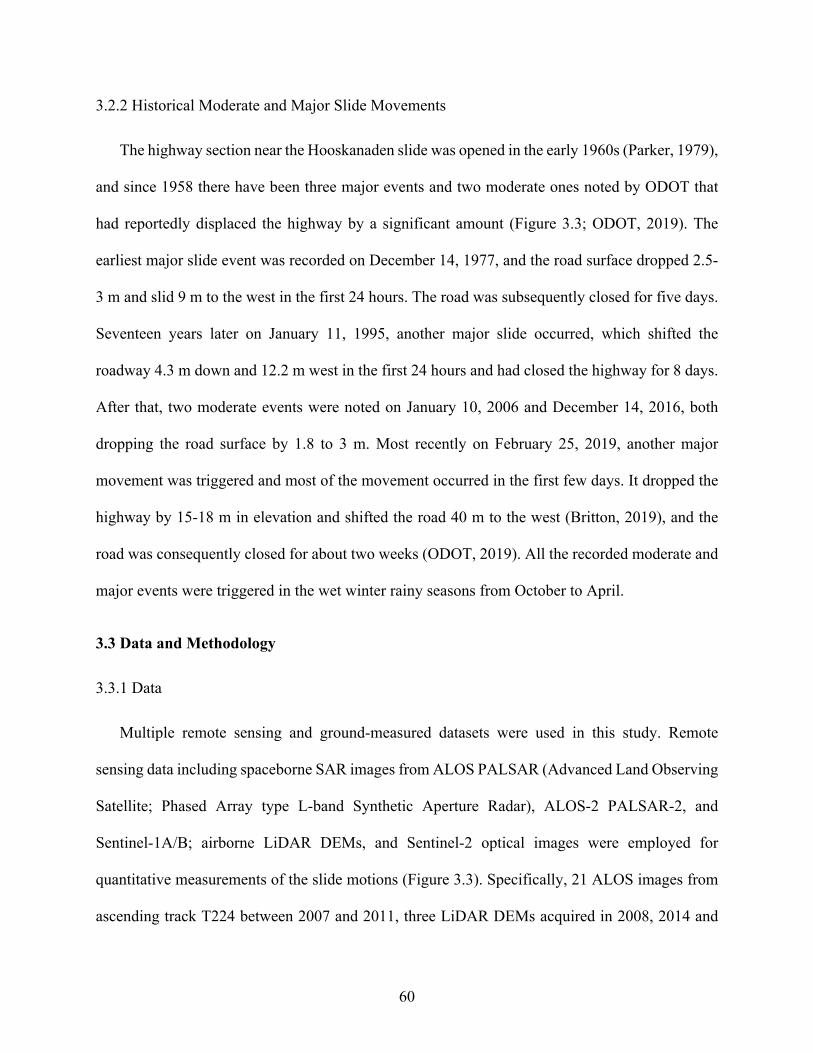
60
3.2.2 Historical Moderate and Major Slide Movements
The highway section near the Hooskanaden slide was opened in the early 1960s (Parker, 1979),
and since 1958 there have been three major events and two moderate ones noted by ODOT that
had reportedly displaced the highway by a significant amount (Figure 3.3; ODOT, 2019). The
earliest major slide event was recorded on December 14, 1977, and the road surface dropped 2.5-
3 m and slid 9 m to the west in the first 24 hours. The road was subsequently closed for five days.
Seventeen years later on January 11, 1995, another major slide occurred, which shifted the
roadway 4.3 m down and 12.2 m west in the first 24 hours and had closed the highway for 8 days.
After that, two moderate events were noted on January 10, 2006 and December 14, 2016, both
dropping the road surface by 1.8 to 3 m. Most recently on February 25, 2019, another major
movement was triggered and most of the movement occurred in the first few days. It dropped the
highway by 15-18 m in elevation and shifted the road 40 m to the west (Britton, 2019), and the
road was consequently closed for about two weeks (ODOT, 2019). All the recorded moderate and
major events were triggered in the wet winter rainy seasons from October to April.
3.3 Data and Methodology
3.3.1 Data
Multiple remote sensing and ground-measured datasets were used in this study. Remote
sensing data including spaceborne SAR images from ALOS PALSAR (Advanced Land Observing
Satellite; Phased Array type L-band Synthetic Aperture Radar), ALOS-2 PALSAR-2, and
Sentinel-1A/B; airborne LiDAR DEMs, and Sentinel-2 optical images were employed for
quantitative measurements of the slide motions (Figure 3.3). Specifically, 21 ALOS images from
ascending track T224 between 2007 and 2011, three LiDAR DEMs acquired in 2008, 2014 and
61
2016 (OLC, 2020), and 84 Sentinel-1A/B images from ascending track T35 between 2016 and
2019 were used altogether to retrieve the long-term displacement history of the Hooskanaden slide
from February 2007 to November 2019. Two Sentinel-2 images acquired on January 2019 and
March 2019, and 10 Sentinel-1A/B images between January 2019 and March 2019 were used to
reconstruct the three-dimensional displacement field of the February 2019 major movement. The
68-meter-deep borehole inclinometer observations with 0.5 m vertical intervals between December
2017 and January 2018 were used to reveal the subsurface motion dynamics of the slide before the
inclinometer was destroyed by slide movement (Castro et al., 2019). In addition, space-captured
SMAP level-4 soil moisture with 9×9 km grid size from 2015 to 2019 (Entekhabi et al. 2014) and
daily precipitation from a ground station located 12 km southwest of the slide from December
1994 to March 2020 (WRCC, 2020) were used to provide hydrological observations.
Figure 3.3 Historical moderate (smaller star) and major movements (bigger star), and time spans of remote sensing and ground-based data as shown by the timeline and corresponding data processing methods.
62
3.3.2 InSAR
The InSAR method incorporate the phase information of SAR imagery to allow millimeter-
scale displacement measurements along the LOS (line-of-sight) direction, and we used this
technique to quantify the long-term time-series of slide displacement. The LiDAR DEM acquired
in 2008 was used during interferogram generation using the GAMMA software (Werner et al.,
2000), and the stratified tropospheric artifacts associated with surface topography were removed
before phase unwrapping. Potential artifacts sourcing from regional soil moisture change and
turbulent troposphere in each interferogram were removed by subtracting the InSAR phase of a
common reference region (16×16 pixels after multi-looking). This reference region is stable, very
close to the landslide (within one kilometer), and has constantly high coherence (greater than 0.7).
The InSAR method was applied to the ALOS and Sentinel-1A/B SAR datasets, and the multi-
looking factors were set as 3×7 (range by azimuth) and 5×2, respectively. Accuracy of InSAR
measurement can be quantified based on the coherence (Rodriguez and Martin, 1992; Lu and
Dzurisin, 2014):
σ =λ4:
ó1
2òâ(1 − P*)P*
(3.1)
where - is the uncertainty of InSAR measurements, 1 the radar wavelength, ò and â the window
sizes for the coherence estimation, and P the coherence. Time-series measurements were achieved
by using a coherence-weighted small baseline subset (SBAS) method (Tarantola, 2005; Tong and
Schmidt, 2013). In matrix form, the time-series inversion problem can be expressed as ôö = õ,
where ô is a matrix in the size of [Z × D + 1] entailing InSAR observations and physical
constraints, ö a matrix containing incremental displacements, and õ the displacement
63
observations of every interferogram. Z is the number of interferograms and D the number of
temporal increments. The equation can be expanded as:
⎣⎢⎢⎢⎡1 1 0 … †%)0 1 1 … †%*… … … … …
1/∆X) −1/∆X) 0 … 00 1/∆X* −1/∆X* … 0 ⎦
⎥⎥⎥⎤
§
!)!*…!3∆ℎ
• =
⎣⎢⎢⎡â)â*…00 ⎦⎥⎥⎤(3.2)
where %$ and ∆X$ is the perpendicular baseline and time interval of the 6th interferogram,
respectively. † is a scaling factor determined by radar wavelength and the relative location between
the satellite and ground targets. By introducing a weight matrix ¶ = .6Yä{P), P*, P7, … , P2}, the
incremental displacements can be solved as:
ö = (ô@¶ô);)ô@¶õ(3.3)
where ô@denotes the transpose of ô. The covariance matrix of ö can be estimated as:
ß = (ô@¶ô);)-®*(3.4)
where -®* is the variance of the InSAR measurements. The small-baseline interferograms used for
time-series inversion were selected by setting a minimum coherence threshold of 0.4 for the L-
band ALOS-1/2 SAR images and 0.2 for the C-band Sentinel-1A/B images before any filtering. A
32×32 moving window was used for coherence estimation, which corresponds to a minimum
measurement uncertainty of ~1.4 mm for ALOS/ALOS-2 and ~0.7 mm for Sentinel-1A/B
interferograms.
3.3.3 Pixel Offset Tracking
Pixel offset tracking that uses the normalized cross correlation (Bernstein and Colby, 1983;
Scambos et al., 1992) to identify matched features and track the offsets between the features is
another method to quantitatively measure landslide movements from remote sensing data. The
64
achievable accuracy -LM of offset estimation via cross correlation is given as equation (3.5) based
on the Cramer-Rao bound (Bamler and Eineder, 2005):
-LM = ó3
2òâS1 − ã*
:ã∙ -/$=(3.5)
where ò and â are window sizes for cross correlation. ã is the cross-correlation coefficient, and
-/$= the pixel resolution. A 32 × 32 window was used for cross correlation of all data (note that
the window size must be two times greater than the to-be-measured displacement), and thresholds
of cross-correlation coefficient were set to 0.2 for Sentinel-1 images, and 0.4 for Sentinel-2 and
LiDAR data. Hence, the measurement accuracy ranges from 0.01 m for the 0.35-meter-resolution
LiDAR DEMs, 0.28 m for the 10-meter-resolution Sentinel-2 images, to 0.8 m for the 14-meter-
resolution Sentinel-1 images in azimuth direction.
Offset tracking was applied to LiDAR DEMs, Sentinel-1A/B SAR images, and Sentinel-2
optical images in this investigation. In contrast to the high-accuracy InSAR that uses phase
information, pixel offset tracking of SAR data uses backscattered intensities and provides a rather
lower accuracy. However, SAR offset tracking works better for measuring high-gradient
displacement that could potentially cause decorrelation and phase unwrapping errors for InSAR.
To enhance the performance of pixel offset tracking, varied preprocessing was implemented on
Sentinel-1A/B SAR data, Sentinel-2 optical images, and LiDAR DEMs.
3.3.3.1 Preprocessing of Sentinel-1/2 images
We averaged multiple Sentinel-1A/B SAR images to reduce the speckle noises and applied
oversampling on the azimuth direction. The 10-m-resolution Sentinel-2 images were oversampled
65
on both northing and easting directions, and both red and near-infrared bands of the multi-band
Sentinel-2 images were combined to enhance ground features by calculating ÄG (simple ratio):
ÄG = ò©G/G(3.6)
where ò©G and G denote the near-infrared and red band respectively. The simple ratio takes
advantage of the relationship between high absorption by chlorophyll of red radiant energy and
high reflectance of near-infrared energy for healthy leaves and plant canopies (Ollinger, 2011),
and can therefore particularly highlight ground features composed of healthy vegetation and
augment the performance of offset tracking.
Specifically, five Sentinel-1A/B SAR images acquired before the event between January 1,
2019 and February 18, 2019 were averaged to form one SAR intensity image named 20190218.ave
(Figure 3.4a), while another five acquired after the event between March 14, 2019 and May 1,
2019 were averaged to form an image named 20190314.ave (Figure 3.4b). Original 2.3 m × 14 m
(range by azimuth) pixel-sized Sentinel-1A/B images were oversampled in the range direction to
2.3 m × 2.8 m pixel size before offset tracking. Pixel offset tracking was implemented on the
simple ratio (equation 3.6) of Sentinel-2 images acquired on January 31, 2019 and March 2, 2019.
An oversampling factor of four was applied to both northing and easting directions (Figures 3.4d,
e).
3.3.3.2 Preprocessing of LiDAR DEMs
We applied pixel offset tracking of LiDAR DEMs on the elevation gradients instead of the
elevations, as elevation gradient can better preserve topographical features than the elevation itself
when vertical deformation exists. No oversampling was applied to the LiDAR DEM gradients
before offset tracking. The elevation gradient ™ was calculated as:
66
™ = óF´Ñ´iL*
+ F´Ñ´jL*
(3.7)
where Ñ denotes the elevation, and i and j represent the easting and northing directions,
respectively. The pixelwise finite difference approximations of elevation gradient for pixel Ñ(6, 8)
are expressed as:
™(6, 8) = óFÑ$J),9 − Ñ$;),9
2ΔiL*
+ FÑ$,9J) − Ñ$,9;)
2ΔjL*
(3.8)
where Δi and Δj are pixel size in i and j directions, respectively. The gradient along the edges
of the matrix is calculated with single-sided differences.
3.3.4 Reconstruction of Three-dimensional Displacement Field
Three-dimensional displacement field of major slides can be reconstructed by combining pixel
offset tracking results from both Sentinel-1A/B SAR data and Sentinel-2 optical images. Defining
K as the radar incidence angle, 5 the satellite heading angle and ¨ = [R,ò, ≠]@ as the pixelwise
displacement vector consisting of northing, easting, and upward components, respectively, ¨ is
related to the measured offsets as:
o ∙ ¨ = r(3.9)
where o is the unit vector of pixel offsets in the Rò≠ coordinate, and r is the measured pixel offsets
from both Sentinel-1A/B and Sentinel-2 images. Equation (3.9) can be expanded as:
§
−sin K cos5 sin K sin5 cos Ksin5 cos5 00 1 01 0 0
• ∙ }Rò≠~ =
⎣⎢⎢⎢⎡É3))É3)*+É3*,É3*- ⎦
⎥⎥⎥⎤(3.10)
67
where É3)_M, É3)_OP, É3*_G, and É3*_Q denote offset measurements from Sentinel-1A/B images in
azimuth and range directions, and that from Sentinel-2 images on northing and easting directions,
respectively. A weighted least squares solution was employed to solve equation (3.10). Similar to
equations (3.3) and (3.4), the 3D vector components can be obtained as ¨ = (o@Æo);)o@Ær by
introducing a diagonal weight matrix Æ based on varied accuracy of the offset measurements. The
covariance matrix of ¨ can be estimated as Ø = (o@Æo);)$∞*, where $∞
* is the variance of the
offset tracking measurements.
As to LiDAR DEMs, the horizontal displacement vectors can be directly obtained from pixel
offset tracking of two LiDAR DEMs while the vertical deformation is attainable from the elevation
changes of DEM based on the measured horizontal offsets. A three-dimensional deformation field
can therefore be reconstructed.
3.4 Results
3.4.1 Three-dimensional Displacement Field of the February 2019 Event
Reconstructing the three-dimensional displacement field of the major movement on February
25, 2019 was achieved by integrating pixel offset tracking of both Sentinel-1A/B SAR images
from Descending track T13 and Sentinel-2 images. Specifically, the three-dimensional movement
vectors (Figure 3.4c) were calculated by constructing and solving equation (3.10) using the four
independent observations from Sentinel-1/2 data. The associated uncertainties of the inverted 3D
motion vectors are depicted in Figure 3.5. Note that each arrow in Figure 3.4c represents the
average horizontal displacement of a 14×14 array of adjacent pixels, which corresponds to a 32 m
× 39 m area on the ground surface. The results show that the 2019 February major slide mainly
moved along the downslope direction with an aspect of 229˚ (clockwise from north), though the
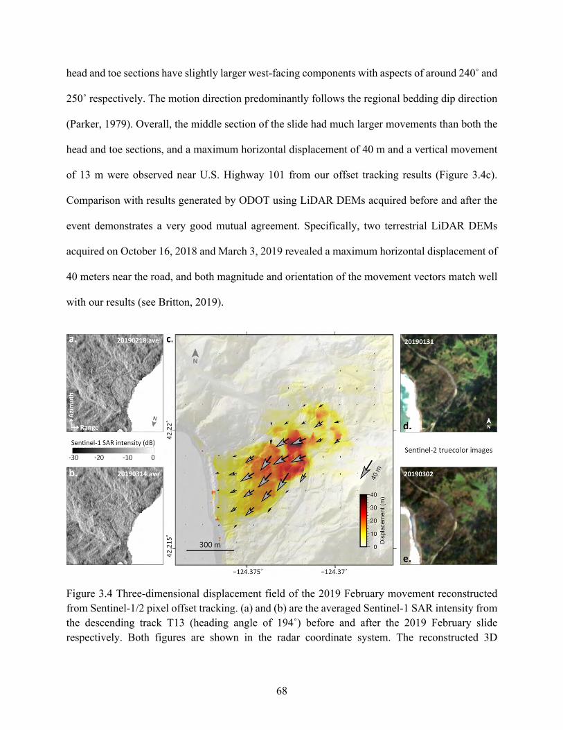
68
head and toe sections have slightly larger west-facing components with aspects of around 240˚ and
250˚ respectively. The motion direction predominantly follows the regional bedding dip direction
(Parker, 1979). Overall, the middle section of the slide had much larger movements than both the
head and toe sections, and a maximum horizontal displacement of 40 m and a vertical movement
of 13 m were observed near U.S. Highway 101 from our offset tracking results (Figure 3.4c).
Comparison with results generated by ODOT using LiDAR DEMs acquired before and after the
event demonstrates a very good mutual agreement. Specifically, two terrestrial LiDAR DEMs
acquired on October 16, 2018 and March 3, 2019 revealed a maximum horizontal displacement of
40 meters near the road, and both magnitude and orientation of the movement vectors match well
with our results (see Britton, 2019).
Figure 3.4 Three-dimensional displacement field of the 2019 February movement reconstructed from Sentinel-1/2 pixel offset tracking. (a) and (b) are the averaged Sentinel-1 SAR intensity from the descending track T13 (heading angle of 194˚) before and after the 2019 February slide respectively. Both figures are shown in the radar coordinate system. The reconstructed 3D
69
displacement field is illustrated in (c) with arrows showing movement direction and relative magnitude. (d) and (e) are the two Sentinel-2 truecolor images used for pixel offset tracking.
3.4.2 Movement Rate from Airborne LiDAR DEMs
We applied pixel offset tracking to the three publicly accessible LiDAR DEMs from the
Oregon Lidar Consortium (OLC, 2020) to reveal the long-term movement rate of the Hooskanaden
slide. The three freely downloadable LiDAR DEMs with a vertical RSME (Root-mean-square
error) of 4.6 mm were acquired on 20081017 (YYYYMMDD), 20140730, and 20160501.
However, the three DEMs can only form two pairs (2008-2014 and 2008-2016) for pixel offset
tracking as the 2014 and 2016 LiDAR DEMs barely overlap (Figures 3.6a, b, c).
As shown in Fig 3.6d, the slide section above the road had moved downslope at about 35 cm/yr
from 2008 to 2014, and the movement direction resembles that of the 2019 February event. Across
the data-missing area below the highway, the displacement rate starts from 30 cm/yr and gradually
decreases towards the coastline. A similar movement pattern was also observed from the 2008-
2016 LiDAR DEM offsets (Figure 3.6e), and much larger motion rates of 45 cm/yr were captured
slightly below the road. The displacement directions remain almost identical during both the 2008-
2014 and 2008-2016 periods. In contrast, the 2019 February event has much smaller south-
orientating components at the slide toe than the slow motions between 2008 and 2016 (Figures
3.4c, 3.6), which suggest that the 2019 major event and the slow motions might have occurred on
different slip surfaces. Various slickensides found in the borehole samples had confirmed the
existence of multiple slip surfaces within the slide body (Figure 3.2a). Moreover, it is also indicated
by the varied vertical slip angles primarily near the road (Figures 3.6f, g, h). The slip angle is
defined as the angle between the displacement vector and the horizontal plane:
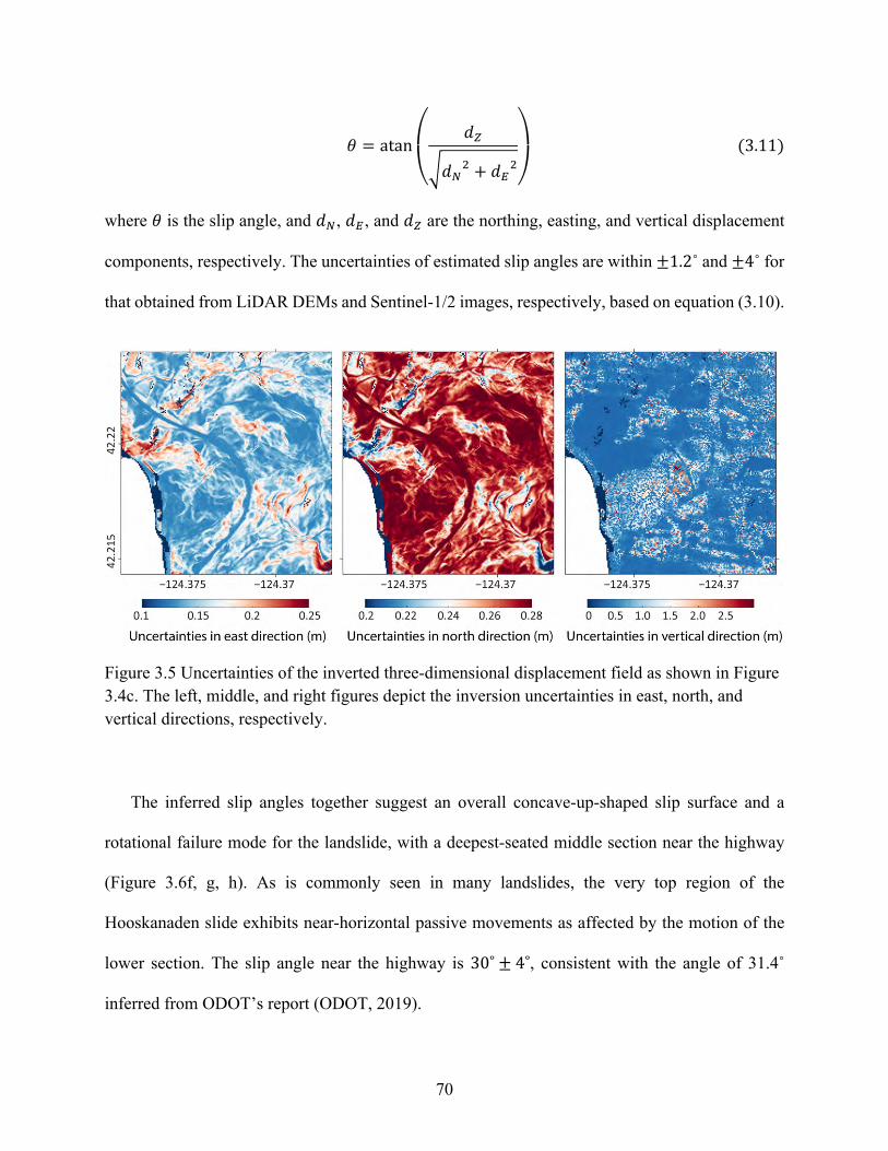
70
K = atan
⎝
⎛ .P
≥.G* + .Q
*⎠
⎞(3.11)
where K is the slip angle, and .G, .Q, and .P are the northing, easting, and vertical displacement
components, respectively. The uncertainties of estimated slip angles are within ±1.2˚ and ±4˚ for
that obtained from LiDAR DEMs and Sentinel-1/2 images, respectively, based on equation (3.10).
Figure 3.5 Uncertainties of the inverted three-dimensional displacement field as shown in Figure 3.4c. The left, middle, and right figures depict the inversion uncertainties in east, north, and vertical directions, respectively.
The inferred slip angles together suggest an overall concave-up-shaped slip surface and a
rotational failure mode for the landslide, with a deepest-seated middle section near the highway
(Figure 3.6f, g, h). As is commonly seen in many landslides, the very top region of the
Hooskanaden slide exhibits near-horizontal passive movements as affected by the motion of the
lower section. The slip angle near the highway is 30˚ ± 4˚, consistent with the angle of 31.4˚
inferred from ODOT’s report (ODOT, 2019).
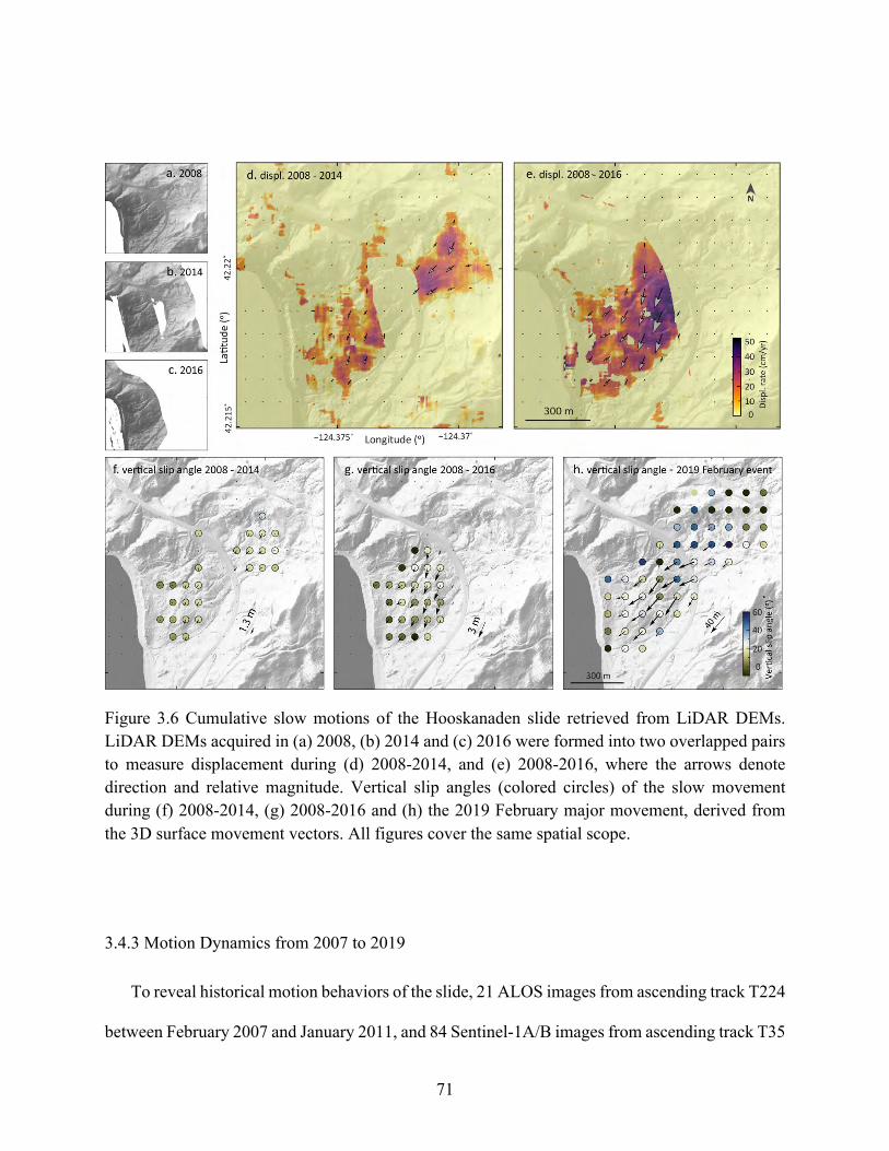
71
Figure 3.6 Cumulative slow motions of the Hooskanaden slide retrieved from LiDAR DEMs. LiDAR DEMs acquired in (a) 2008, (b) 2014 and (c) 2016 were formed into two overlapped pairs to measure displacement during (d) 2008-2014, and (e) 2008-2016, where the arrows denote direction and relative magnitude. Vertical slip angles (colored circles) of the slow movement during (f) 2008-2014, (g) 2008-2016 and (h) the 2019 February major movement, derived from the 3D surface movement vectors. All figures cover the same spatial scope.
3.4.3 Motion Dynamics from 2007 to 2019
To reveal historical motion behaviors of the slide, 21 ALOS images from ascending track T224
between February 2007 and January 2011, and 84 Sentinel-1A/B images from ascending track T35
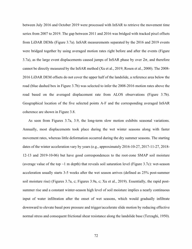
72
between July 2016 and October 2019 were processed with InSAR to retrieve the movement time
series from 2007 to 2019. The gap between 2011 and 2016 was bridged with tracked pixel offsets
from LiDAR DEMs (Figure 3.7a). InSAR measurements separated by the 2016 and 2019 events
were bridged together by using averaged motion rates right before and after the events (Figure
3.7a), as the large event displacements caused jumps of InSAR phase by over 2:, and therefore
cannot be directly measured by the InSAR method (Xu et al., 2019; Rosen et al., 2000). The 2008-
2016 LiDAR DEM offsets do not cover the upper half of the landslide, a reference area below the
road (blue dashed box in Figure 3.7b) was selected to infer the 2008-2016 motion rates above the
road based on the averaged displacement rate from ALOS observations (Figure 3.7b).
Geographical location of the five selected points A-F and the corresponding averaged InSAR
coherence are shown in Figure 3.8.
As seen from Figures 3.7a, 3.9, the long-term slow motion exhibits seasonal variations.
Annually, most displacements took place during the wet winter seasons along with faster
movement rates, whereas little deformation occurred during the dry summer seasons. The starting
dates of the winter acceleration vary by years (e.g., approximately 2016-10-27, 2017-11-27, 2018-
12-13 and 2019-10-06) but have good correspondences to the root-zone SMAP soil moisture
(average value of the top ~1 m depth) that reveals soil saturation level (Figure 3.7c): wet-season
acceleration usually starts 3-5 weeks after the wet season arrives (defined as 25% post-summer
soil moisture rise) (Figures 3.7a, c; Figures 3.9a, c; Xu et al., 2019). Essentially, the rapid post-
summer rise and a constant winter-season high level of soil moisture implies a nearly continuous
input of water infiltration after the onset of wet seasons, which would gradually infiltrate
downward to elevate basal pore pressure and trigger/accelerate slide motion by reducing effective
normal stress and consequent frictional shear resistance along the landslide base (Terzaghi, 1950).
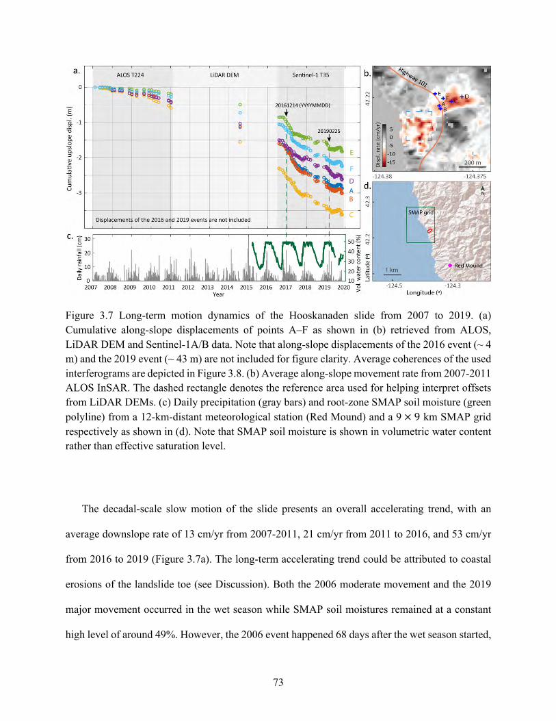
73
Figure 3.7 Long-term motion dynamics of the Hooskanaden slide from 2007 to 2019. (a) Cumulative along-slope displacements of points A–F as shown in (b) retrieved from ALOS, LiDAR DEM and Sentinel-1A/B data. Note that along-slope displacements of the 2016 event (~ 4 m) and the 2019 event (~ 43 m) are not included for figure clarity. Average coherences of the used interferograms are depicted in Figure 3.8. (b) Average along-slope movement rate from 2007-2011 ALOS InSAR. The dashed rectangle denotes the reference area used for helping interpret offsets from LiDAR DEMs. (c) Daily precipitation (gray bars) and root-zone SMAP soil moisture (green polyline) from a 12-km-distant meteorological station (Red Mound) and a 9× 9 km SMAP grid respectively as shown in (d). Note that SMAP soil moisture is shown in volumetric water content rather than effective saturation level.
The decadal-scale slow motion of the slide presents an overall accelerating trend, with an
average downslope rate of 13 cm/yr from 2007-2011, 21 cm/yr from 2011 to 2016, and 53 cm/yr
from 2016 to 2019 (Figure 3.7a). The long-term accelerating trend could be attributed to coastal
erosions of the landslide toe (see Discussion). Both the 2006 moderate movement and the 2019
major movement occurred in the wet season while SMAP soil moistures remained at a constant
high level of around 49%. However, the 2006 event happened 68 days after the wet season started,
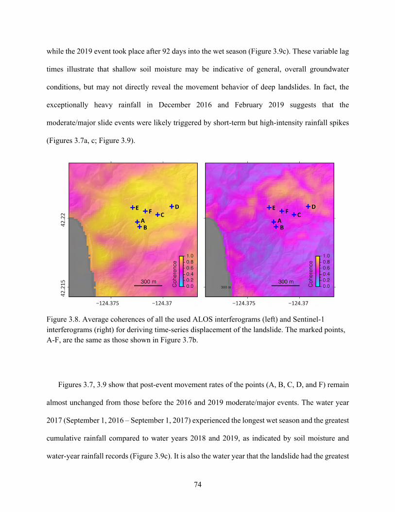
74
while the 2019 event took place after 92 days into the wet season (Figure 3.9c). These variable lag
times illustrate that shallow soil moisture may be indicative of general, overall groundwater
conditions, but may not directly reveal the movement behavior of deep landslides. In fact, the
exceptionally heavy rainfall in December 2016 and February 2019 suggests that the
moderate/major slide events were likely triggered by short-term but high-intensity rainfall spikes
(Figures 3.7a, c; Figure 3.9).
Figure 3.8. Average coherences of all the used ALOS interferograms (left) and Sentinel-1 interferograms (right) for deriving time-series displacement of the landslide. The marked points, A-F, are the same as those shown in Figure 3.7b.
Figures 3.7, 3.9 show that post-event movement rates of the points (A, B, C, D, and F) remain
almost unchanged from those before the 2016 and 2019 moderate/major events. The water year
2017 (September 1, 2016 – September 1, 2017) experienced the longest wet season and the greatest
cumulative rainfall compared to water years 2018 and 2019, as indicated by soil moisture and
water-year rainfall records (Figure 3.9c). It is also the water year that the landslide had the greatest
75
annual displacements and non-stop movements even during summer (Figures 3.7a, 3.9a). In
contrast, all six points (A-F) had lower total displacements in both water years 2018 and 2019 and
had temporary movement stoppages in both 2018 and 2019 summers. All the above observations
indicate a strong correlation between precipitation and the landslide’s slow motions.
Figure 3.9 A close-up of the landslide motion dynamics between 2016 and 2019. (a) Cumulative along-slope displacements of three points (A, D, and E as shown in Figure 3.7b), and time lags between arrival of wet seasons and seasonal accelerations from 2016 to 2019. (b) Movement rates of the three points (in consistent colors) obtained from displacement time series using forward difference approximations. (c) Daily rainfall (gray bars), cumulative water-year rainfall starting
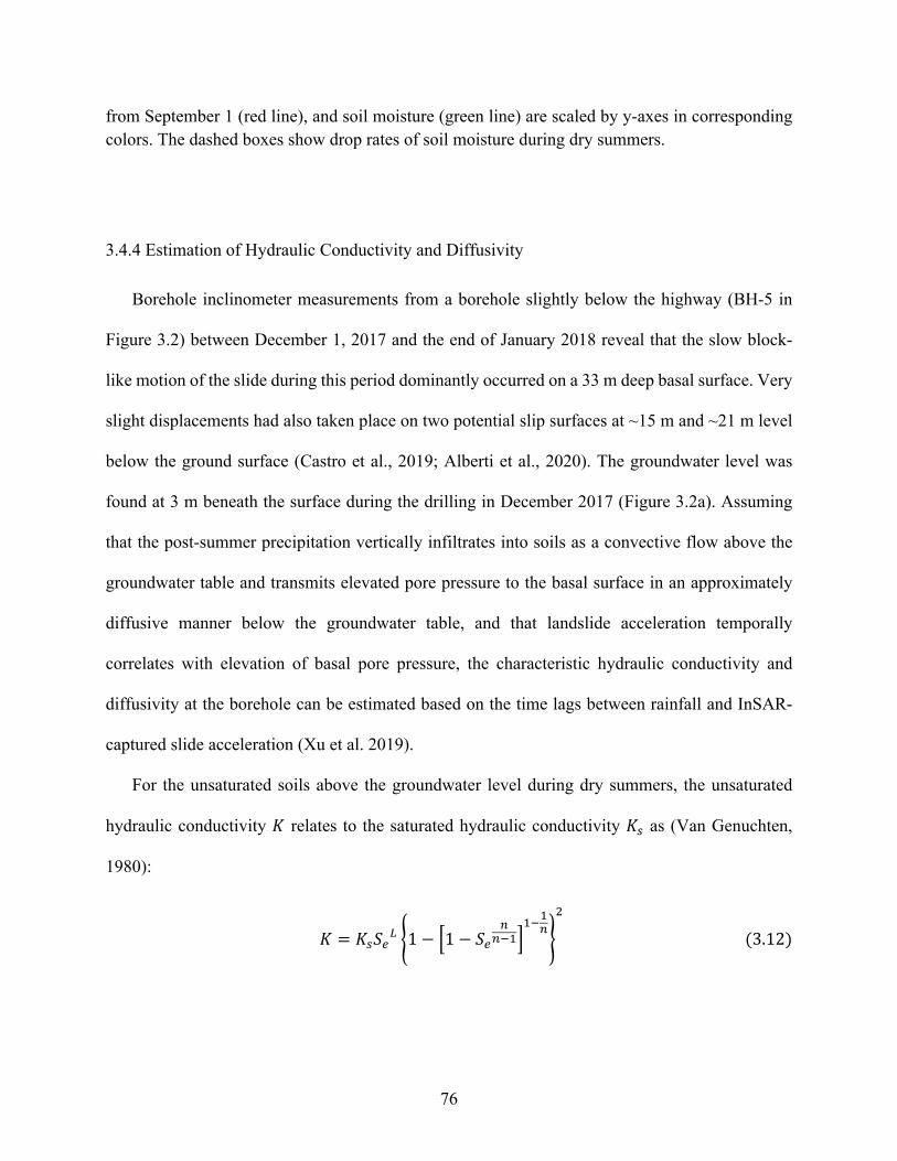
76
from September 1 (red line), and soil moisture (green line) are scaled by y-axes in corresponding colors. The dashed boxes show drop rates of soil moisture during dry summers.
3.4.4 Estimation of Hydraulic Conductivity and Diffusivity
Borehole inclinometer measurements from a borehole slightly below the highway (BH-5 in
Figure 3.2) between December 1, 2017 and the end of January 2018 reveal that the slow block-
like motion of the slide during this period dominantly occurred on a 33 m deep basal surface. Very
slight displacements had also taken place on two potential slip surfaces at ~15 m and ~21 m level
below the ground surface (Castro et al., 2019; Alberti et al., 2020). The groundwater level was
found at 3 m beneath the surface during the drilling in December 2017 (Figure 3.2a). Assuming
that the post-summer precipitation vertically infiltrates into soils as a convective flow above the
groundwater table and transmits elevated pore pressure to the basal surface in an approximately
diffusive manner below the groundwater table, and that landslide acceleration temporally
correlates with elevation of basal pore pressure, the characteristic hydraulic conductivity and
diffusivity at the borehole can be estimated based on the time lags between rainfall and InSAR-
captured slide acceleration (Xu et al. 2019).
For the unsaturated soils above the groundwater level during dry summers, the unsaturated
hydraulic conductivity � relates to the saturated hydraulic conductivity �3 as (Van Genuchten,
1980):
� = �3Ä,C Å1 − q1 − Ä,
22;)u
);)2Ç
*
(3.12)
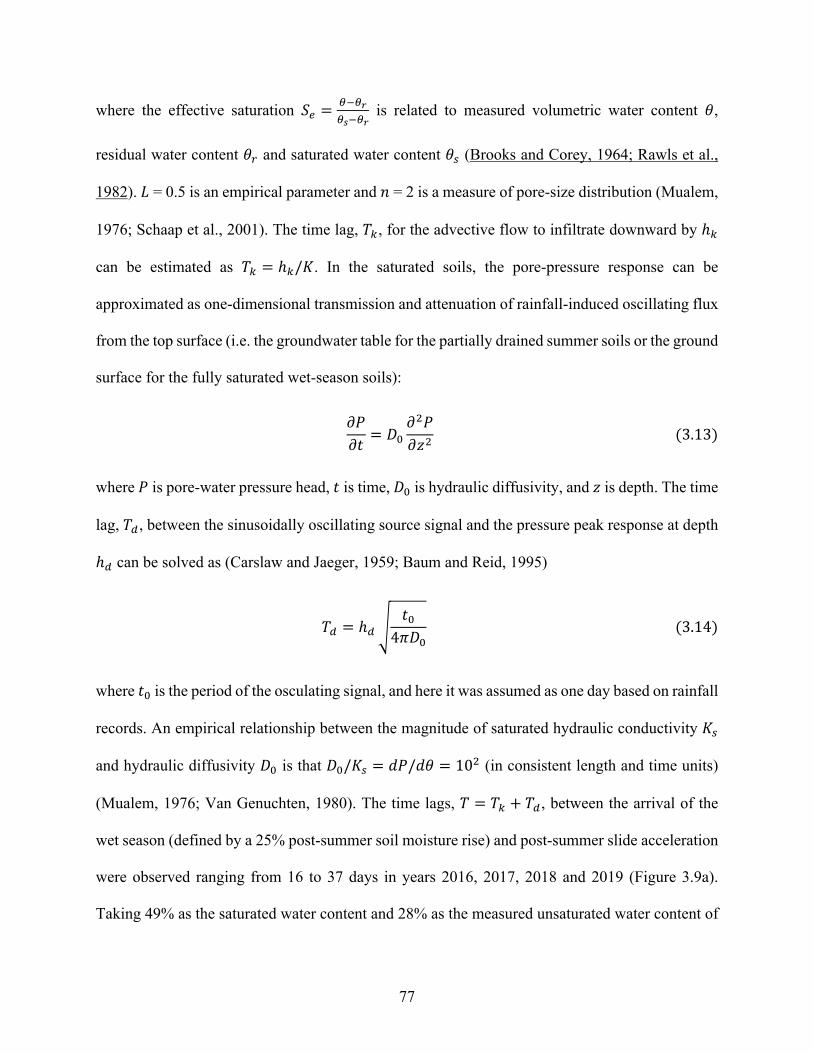
77
where the effective saturation Ä, =R;R.R(;R.
is related to measured volumetric water content K,
residual water content K# and saturated water content K3 (Brooks and Corey, 1964; Rawls et al.,
1982). É = 0.5 is an empirical parameter and Z = 2 is a measure of pore-size distribution (Mualem,
1976; Schaap et al., 2001). The time lag, /B, for the advective flow to infiltrate downward by ℎB
can be estimated as /B = ℎB/�. In the saturated soils, the pore-pressure response can be
approximated as one-dimensional transmission and attenuation of rainfall-induced oscillating flux
from the top surface (i.e. the groundwater table for the partially drained summer soils or the ground
surface for the fully saturated wet-season soils):
´e´X
= Ü!´*e´∑*
(3.13)
where e is pore-water pressure head, X is time, Ü! is hydraulic diffusivity, and ∑ is depth. The time
lag, /+, between the sinusoidally oscillating source signal and the pressure peak response at depth
ℎ+ can be solved as (Carslaw and Jaeger, 1959; Baum and Reid, 1995)
/+ = ℎ+ óX!
4:Ü!(3.14)
where X! is the period of the osculating signal, and here it was assumed as one day based on rainfall
records. An empirical relationship between the magnitude of saturated hydraulic conductivity �3
and hydraulic diffusivity Ü! is that Ü!/�3 = .e/.K = 10* (in consistent length and time units)
(Mualem, 1976; Van Genuchten, 1980). The time lags, / = /B + /+, between the arrival of the
wet season (defined by a 25% post-summer soil moisture rise) and post-summer slide acceleration
were observed ranging from 16 to 37 days in years 2016, 2017, 2018 and 2019 (Figure 3.9a).
Taking 49% as the saturated water content and 28% as the measured unsaturated water content of
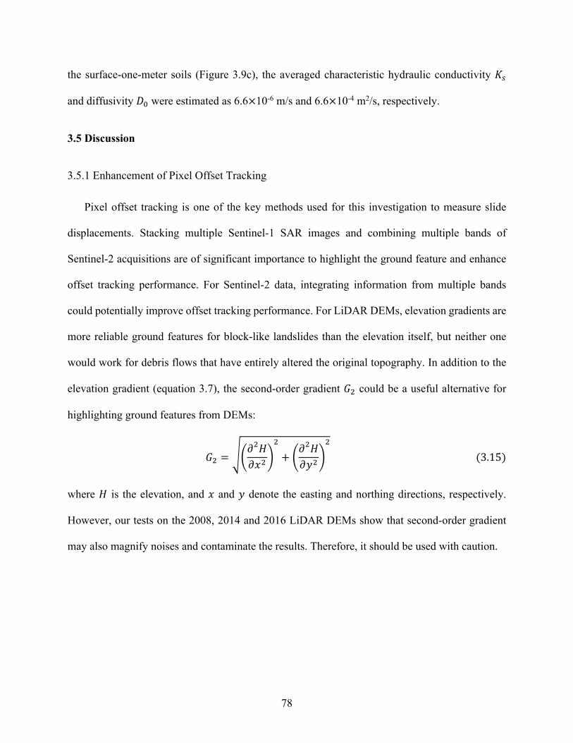
78
the surface-one-meter soils (Figure 3.9c), the averaged characteristic hydraulic conductivity �3
and diffusivity Ü! were estimated as 6.6×10⁻⁶ m/s and 6.6×10⁻⁴ m2/s, respectively.
3.5 Discussion
3.5.1 Enhancement of Pixel Offset Tracking
Pixel offset tracking is one of the key methods used for this investigation to measure slide
displacements. Stacking multiple Sentinel-1 SAR images and combining multiple bands of
Sentinel-2 acquisitions are of significant importance to highlight the ground feature and enhance
offset tracking performance. For Sentinel-2 data, integrating information from multiple bands
could potentially improve offset tracking performance. For LiDAR DEMs, elevation gradients are
more reliable ground features for block-like landslides than the elevation itself, but neither one
would work for debris flows that have entirely altered the original topography. In addition to the
elevation gradient (equation 3.7), the second-order gradient ™* could be a useful alternative for
highlighting ground features from DEMs:
™* = ó∏´*Ñ´i*
π*
+ ∏´*Ñ´j*
π*
(3.15)
where Ñ is the elevation, and i and j denote the easting and northing directions, respectively.
However, our tests on the 2008, 2014 and 2016 LiDAR DEMs show that second-order gradient
may also magnify noises and contaminate the results. Therefore, it should be used with caution.
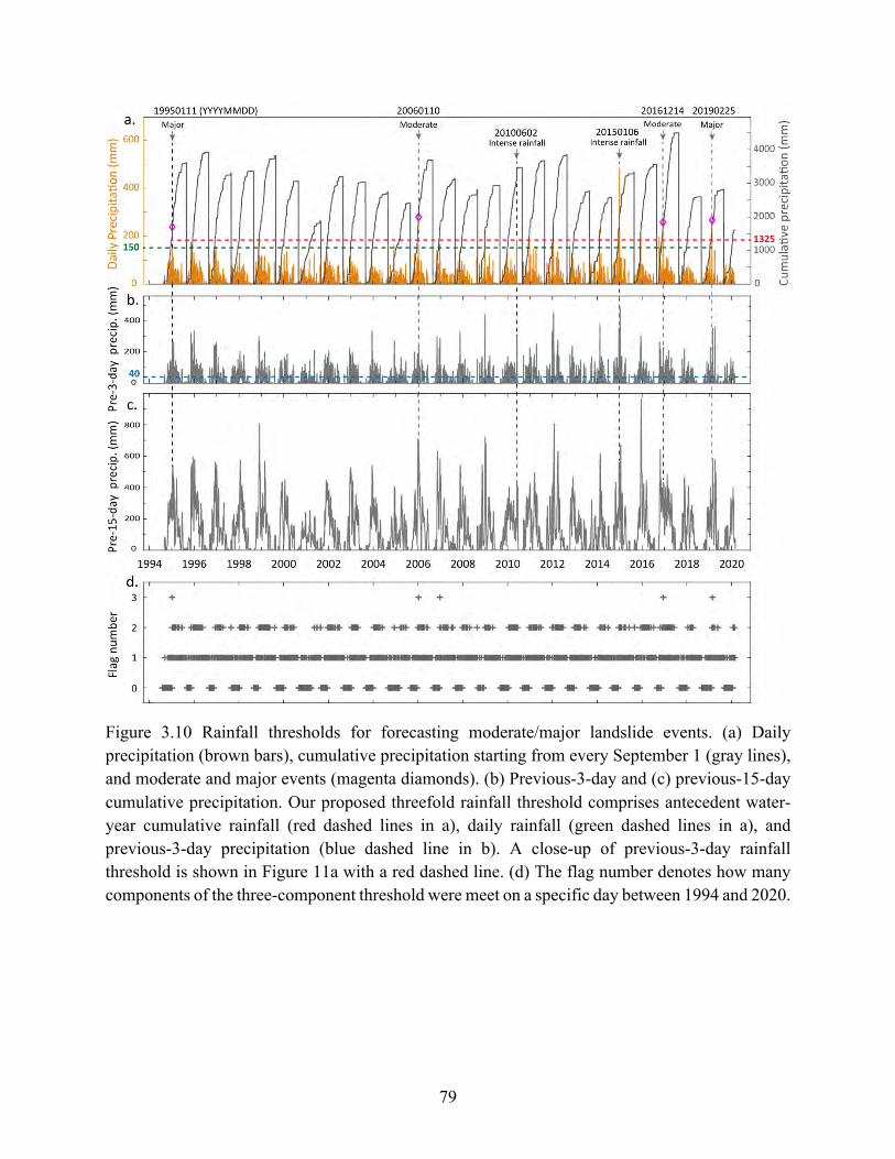
79
Figure 3.10 Rainfall thresholds for forecasting moderate/major landslide events. (a) Daily precipitation (brown bars), cumulative precipitation starting from every September 1 (gray lines), and moderate and major events (magenta diamonds). (b) Previous-3-day and (c) previous-15-day cumulative precipitation. Our proposed threefold rainfall threshold comprises antecedent water-year cumulative rainfall (red dashed lines in a), daily rainfall (green dashed lines in a), and previous-3-day precipitation (blue dashed line in b). A close-up of previous-3-day rainfall threshold is shown in Figure 11a with a red dashed line. (d) The flag number denotes how many components of the three-component threshold were meet on a specific day between 1994 and 2020.
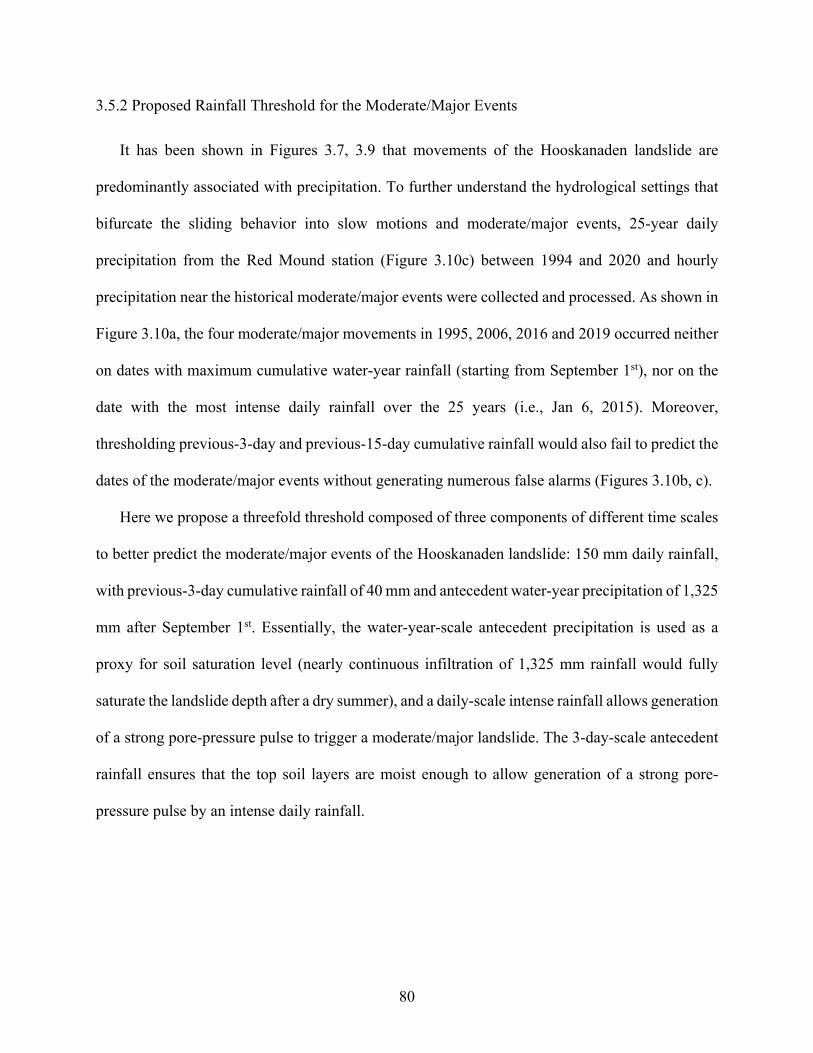
80
3.5.2 Proposed Rainfall Threshold for the Moderate/Major Events
It has been shown in Figures 3.7, 3.9 that movements of the Hooskanaden landslide are
predominantly associated with precipitation. To further understand the hydrological settings that
bifurcate the sliding behavior into slow motions and moderate/major events, 25-year daily
precipitation from the Red Mound station (Figure 3.10c) between 1994 and 2020 and hourly
precipitation near the historical moderate/major events were collected and processed. As shown in
Figure 3.10a, the four moderate/major movements in 1995, 2006, 2016 and 2019 occurred neither
on dates with maximum cumulative water-year rainfall (starting from September 1st), nor on the
date with the most intense daily rainfall over the 25 years (i.e., Jan 6, 2015). Moreover,
thresholding previous-3-day and previous-15-day cumulative rainfall would also fail to predict the
dates of the moderate/major events without generating numerous false alarms (Figures 3.10b, c).
Here we propose a threefold threshold composed of three components of different time scales
to better predict the moderate/major events of the Hooskanaden landslide: 150 mm daily rainfall,
with previous-3-day cumulative rainfall of 40 mm and antecedent water-year precipitation of 1,325
mm after September 1st. Essentially, the water-year-scale antecedent precipitation is used as a
proxy for soil saturation level (nearly continuous infiltration of 1,325 mm rainfall would fully
saturate the landslide depth after a dry summer), and a daily-scale intense rainfall allows generation
of a strong pore-pressure pulse to trigger a moderate/major landslide. The 3-day-scale antecedent
rainfall ensures that the top soil layers are moist enough to allow generation of a strong pore-
pressure pulse by an intense daily rainfall.
81
Figure 3.11 Daily and hourly precipitation near special dates. (a) Daily and (b) hourly rainfall near the moderate and major landslide events, where negative x-axis values represent days/hours before the event. (c) Daily and (d) hourly rainfall for two special dates when intense rainfall did not trigger larger landslide movement. Blue lines in (a) and (c) represent previous-3-day cumulative rainfall, while those in (b) and (d) denote previous-48-hour cumulative precipitation. The red dashed line in (a) marks the minimum previous-3-day cumulative precipitation in our proposed threefold rainfall threshold.
The proposed threefold threshold can accurately predict the dates for the four moderate/major
events between 1995 and 2020 with only one false alarm on 20061215 [YYYYMMDD] (Figures
3.10a,d, 3.11a). Worth mentioning is that the 3-day-scale rainfall threshold of 40 mm successfully
82
eliminated two potential false alarms on dates with over 150 mm daily rainfall (i.e., 20100602 and
20150106). A detailed look of the daily and hourly rainfall records reveals that the intense
precipitation on 20100602 occurred after seven consecutive dry days, and the extremely intense
precipitation on 20150106 (481.58 mm of rainfall fell within one hour) also occurred after 12
continuously dry days (Figures 3.11c, d). The real pore-pressure pulse caused by the storms could
have been significantly reduced by what might be expected due to rainwater absorption within the
upper, drier part of the landslide and due to overland flows (rainfall rate exceeds K), and
consequently was not able to trigger a moderate/major movement. Using the averaged drop rate of
soil moisture during summers (see black dashed boxes in Figure 3.9c), we estimated that soil
moisture would drop from 0.49 to 0.484 after three consecutive dry days, and the corresponding
unsaturated hydraulic conductivity � would drop by 30% from 6.6×10⁻⁶ m/s to 4.64×10⁻⁶ m/s
(Figure 3.12c) based on equation 3.12. An empirical 40 mm threshold of previous-3-day
cumulative rainfall was therefore set to avoid false alarms caused by dried upper soil layers, based
on historical pre-3-day rainfall records (Figures 3.11a, c).
The threshold of the antecedent water-year rainfall is tied to the antecedent groundwater level
and summer soil moisture. Borehole drilling on December 1, 2017 revealed a groundwater level
of 3 m below the surface at the Hooskanaden landslide (Figure 3.2a), and daily logs of a
groundwater well (CURR 819) 23.5 km southeast of the landslide show that groundwater levels
increased from 16.1 m above sea level (water-year low) on September 1, 2017 to 18.4 m (water-
year peak) on April 9, 2018 at the site. It implies a lower bound of groundwater level of -5.3 m at
the landslide site in 2017 summer, and consequently a ~1,325 mm cumulative precipitation to fully
saturate the landslide materials, as SMAP data shows that average soil moisture of the top-one-
meter soils bottoms at 25% during the 2017 summer (Figure 3.9c). The daily rainfall threshold
83
was set empirically based on daily rainfall records of the first moderate/major event (the 1995 one)
shown in Figure 3.10a and can yield accurate forecasting, as validated by the other three later
events in 2006, 2016, and 2019. Note that the moderate/major slides may have been triggered by
an extremely short-term rainfall spike in a rainy day, which may require rainfall records with finer
time scale such as every 5 minutes to be better understood.
Determining the proposed threefold rainfall threshold requires precipitation time-series,
landslide thickness and groundwater depth, hydraulic parameters of the landslide material, and
past landslide motion records (or soil mechanical parameters). These data and parameters can be
obtained through variable means depending on the specific case. Here for the Hooskanaden
landslide we employed primarily remote sensing data and ground-based hydrological
observations, and our methods can be easily adapted for other similar landslides globally to serve
for landslide movement forecasting. Overall, the concept of the “three-component” threshold that
accounts for various hydrological processes could be applicable to many deep-seated landslides,
but the exact threshold for each component must be site-specific and could be derived from field
observations and/or empirical values.
3.5.3 Mechanism of Landslide Motions Modulated by Precipitation and Coastal Erosion
Overall, our analysis has confirmed that both slow motions and moderate/major events of the
Hooskanaden landslide are controlled by precipitation, though the exact processes differ. The slow
motion usually starts 3-5 weeks after the wet season arrives (defined by a 25% post-summer soil
moisture rise), and is controlled by both rainwater infiltration of the top dry layers (unsaturated
during summer) and pore pressure transmission in saturated soils (Figures 3.7a, 3.9a; Xu at al.,
2019). In contrast, moderate/major slide events respond much faster to rainfall pulses, for example,
in approximately 2 days, as the soils are almost saturated in the midst of a wet season and the slide
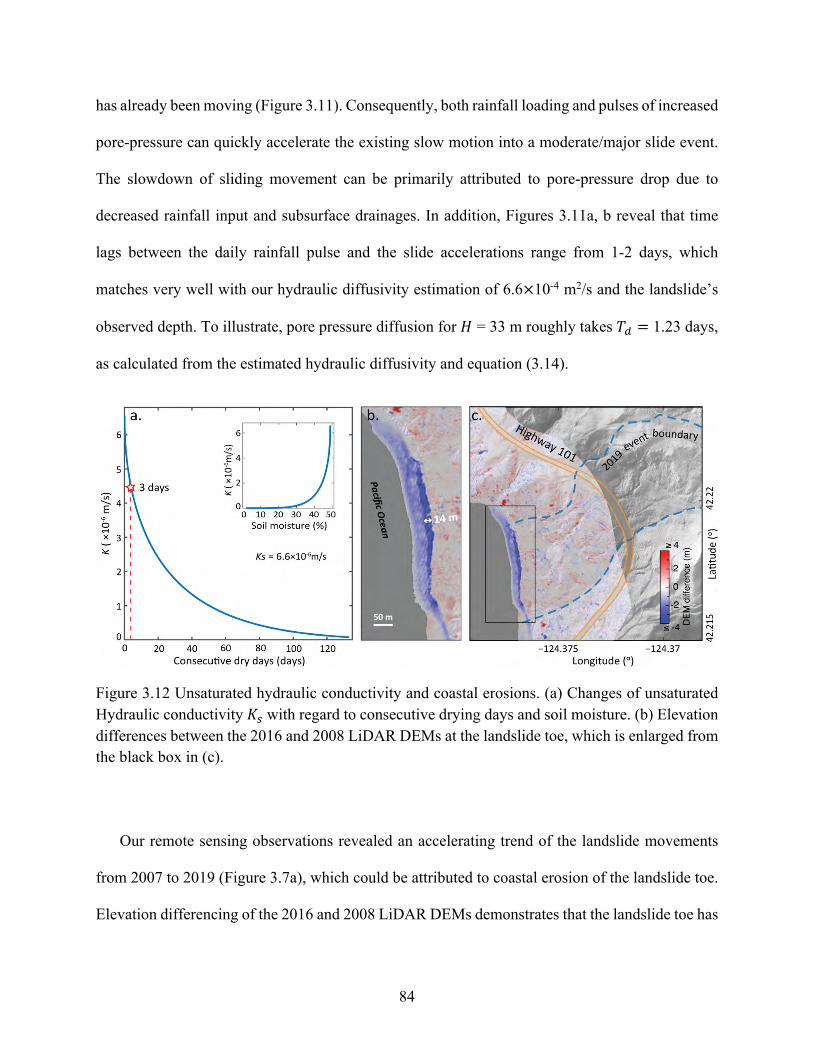
84
has already been moving (Figure 3.11). Consequently, both rainfall loading and pulses of increased
pore-pressure can quickly accelerate the existing slow motion into a moderate/major slide event.
The slowdown of sliding movement can be primarily attributed to pore-pressure drop due to
decreased rainfall input and subsurface drainages. In addition, Figures 3.11a, b reveal that time
lags between the daily rainfall pulse and the slide accelerations range from 1-2 days, which
matches very well with our hydraulic diffusivity estimation of 6.6×10⁻⁴ m2/s and the landslide’s
observed depth. To illustrate, pore pressure diffusion for Ñ = 33 m roughly takes /+ = 1.23 days,
as calculated from the estimated hydraulic diffusivity and equation (3.14).
Figure 3.12 Unsaturated hydraulic conductivity and coastal erosions. (a) Changes of unsaturated Hydraulic conductivity �3 with regard to consecutive drying days and soil moisture. (b) Elevation differences between the 2016 and 2008 LiDAR DEMs at the landslide toe, which is enlarged from the black box in (c).
Our remote sensing observations revealed an accelerating trend of the landslide movements
from 2007 to 2019 (Figure 3.7a), which could be attributed to coastal erosion of the landslide toe.
Elevation differencing of the 2016 and 2008 LiDAR DEMs demonstrates that the landslide toe has
85
undergone significant erosions from 2009 to 2016: ~14 m wide of the coast has elevation drops of
over 4 m. The annual coastline retreat rate at the landslide toe is ~1.9 m/yr, which might have led
to the long-term acceleration of landslide motions by reducing passive resistances.
3.6 Conclusions
Multiple remote sensing datasets and processing methods, borehole measurements, and
hydrological observations have been used in this investigation to understand 12-year motion
dynamics of the Hooskanaden landslide that exhibited both long-term slow movements and short-
term moderate/major slide events. Pixel offset tracking of both Sentinel-1 SAR images and
Sentinel-2 optical images was carried out to reconstruct the three-dimensional displacement field
of the 2019 February major movement. Offsets of LiDAR DEMs were obtained by using elevation
gradients to reveal the 3D motion rates of the landslide between 2008 and 2016. Together with
InSAR processing of ALOS and Sentinel-1 SAR images, a 12-year displacement history of the
Hooskanaden landslide has been retrieved.
Movement rates of the landslide exhibit substantial seasonal variations on an annual scale with
dominating wet-season displacements, and an overall accelerating trend can be seen over the past
decade potentially due to coastal erosion. Pixel offset tracking was successfully applied to the
Sentinel-1/2 images and LiDAR DEMs to recover the three-dimensional displacement field of the
2019 February major movement, and to reveal that the rapid movement and slow motions may
have occurred on slightly different slip surfaces. By using satellite captured SMAP soil moisture
and InSAR derived time lags for post-summer rainfall to trigger the first seasonal sliding
acceleration, the averaged characteristic hydraulic conductivity �3 and diffusivity Ü! of the
landslide materials were estimated as 6.6×10⁻⁶ m/s and 6.6×10⁻⁴ m2/s, respectively. These produce
timing estimations that agree with the observed 2-day time lag for rainfall pulses to trigger the
86
1995, 2016 and 2019 moderate/major movements. Comparison between the motion history and
ground rainfall records demonstrates that thresholding pre-3-day and pre-15-day cumulative
precipitation cannot lead to effective prediction of dates for moderate/major events. In contrast,
more accurate prediction can be achieved by using our proposed threefold threshold of 150 mm
daily rainfall, with previous-3-day cumulative rainfall of 40 mm and antecedent water-year
precipitation of 1,325 mm after September 1st.
Our study demonstrates the utility of integrating multiple remote sensing methods (InSAR and
pixel offset tracking) and datasets (ALOS and Sentinel-1 SAR, Sentinel-2 optical images, and
LiDAR DEMs) to retrieve long-term displacement time series and achieve 3D characterizations of
a landslide, which are of great significance for forecasting the landslide’s future motions (e.g.,
seasonal accelerations and decelerations, the rotation failure mode, and the long-term acceleration
associated with coastal erosion). Furthermore, we propose a new threefold rainfall threshold based
on shallow soil moisture from SMAP and 15-year ground precipitation records to forecast both the
seasonal onsets of creeping motion as well as moderate/major events of the Hooskanaden
landslide. The ability of the proposed threshold has been explained with hydrological modeling
and remote sensing observations. Our approaches for developing the threshold predominantly rely
on remote sensing data and ground precipitation and does not require expensive and labor-
intensive pore-pressure monitoring, and therefore can be easily adapted for other similar landslides
worldwide.
87
ACKNOWLEDGEMENTS
This study benefited from the support provided by Jill DeKoekkoek, Dan Latham, Ben
Leshchinsky, Pete Castro, Audrey Britton, and Tidewater Contractors, Inc. This research was
financially supported by NASA Interdisciplinary Research (IDS) in Earth Science Program
(80NSSC17K0022) and the Shuler-Foscue Endowment at Southern Methodist University. ALOS
PALSAR datasets were copyrighted by the Japan Aerospace Exploration Agency (JAXA) and
provided by Alaska Satellite Facility (ASF). Copernicus Sentinel data 2016-2019 processed by
European Space Agency (ESA) were retrieved from ASF Distributed Active Archive Center
(DAAC). SMAP soil moisture data were provided by the National Aeronautics and Space
Administration (NASA). LiDAR DEMs were accessed from Oregon Lidar Consortium. We thank
Jonathan Perkins, Estelle Chaussard, Noah Finnegan, and one anonymous reviewer for providing
suggestions that improved this manuscript. Data that support this study are available at
https://smu.box.com/v/HooskanadenSlide
88
REFERENCES
Alberti, S., Senogles, A., Kingen, K., Booth, A., Castro, P., DeKoekkoek, J., Glover-Cutter, K., Mohney, C., Olsen, M. and Leshchinsky, B. (2020). The Hooskanaden Landslide: historic and recent surge behavior of an active earthflow on the Oregon Coast. Landslides, 17, 2589–2602.
Angeli, M. G., Gasparetto, P., Menotti, R. M., Pasuto, A., and Silvano, S. (1996). A visco-plastic model for slope analysis applied to a mudslide in Cortina d'Ampezzo, Italy. Quarterly Journal of Engineering Geology and Hydrogeology, 29(3), 233-240.
Bamler, R., and Eineder, M. (2005). Accuracy of differential shift estimation by correlation and split-bandwidth interferometry for wideband and delta-k SAR systems. IEEE Geoscience and Remote Sensing Letters, 2(2), 151-155.
Baum, R. L., and Reid, M.E. (1995). Geology, hydrology, and mechanics of a slow-moving. Clay Shale Slope Instability, 10, 79.
Bernstein, R., and Colby, C. (1983). Image geometry and rectification. Manual of remote sensing, 1, 873-922.
Britton, M. A. (2019). Study of the Hooskanaden Slide Using LiDAR Technology. 2019 Symposium by the Sea. Retrieved from https://www.orurisa.org/resources/Audrey%20McHugh-Britton%20OregonDOT%20Hooskanaden%20Slide.pdf
Brooks, R. H., and Corey, A. T. (1964). Hydraulic properties of porous media. Hydrology Paper, Vol. 3, Colorado State University, Fort Collins.
Carslaw, H. S., and Jaeger, J. C. (1959). Conduction of heat in solids. Clarendon press.
Castro, P., Mohney, C., DeKoekkoek, J., and Cunningham, C. (2019). Hooskanaden Landslide Reconnaissance in Response to 2019 Episodic Movement; Oregon Coast Hwy (US 101) (Hwy. 9, M.P. 343.5), Curry County, Oregon.
Entekhabi, D., Yueh, S., and De Lannoy, G. (2014). SMAP handbook.
Froude, M. J., and Petley, D. (2018). Global fatal landslide occurrence from 2004 to 2016. Natural Hazards and Earth System Sciences, 18, 2161-2181. https://doi.org/10.5194/nhess-18-2161-2018
89
Gasparetto, P., Mosselman, M., and Van Asch, T. W. (1996). The mobility of the Alvera landslide (Cortina d'Ampezzo, Italy). Geomorphology, 15(3-4), 327-335. https://doi.org/10.1016/0169-555X(95)00078-J
Lu, Z., and Dzurisin, D. (2014). InSAR Imaging of Aleutian Volcanoes: Monitoring a Volcanic Arc from Space. Springer: Berlin/Heidelberg, Germany.
Mackey, B. H., and Roering, J. J. (2011). Sediment yield, spatial characteristics, and the long-term evolution of active earthflows determined from airborne LiDAR and historical aerial photographs, Eel River, California. Bulletin, 123(7-8), 1560-1576.
Massey, C. I., Petley, D. N., and McSaveney, M. J. (2013). Patterns of movement in reactivated landslides. Engineering Geology, 159, 1-19.
Mualem, Y. (1976). A new model for predicting the hydraulic conductivity of unsaturated porous media. Water resources research, 12(3), 513-522.
ODOT (Oregon Department of Transportation). (2019). Hooskanaden Slide Update. Retrieved from http://www.co.curry.or.us/2019_05_%20Hooskanaden%20Slide%20Update%20ODOT.pdf
OLC (Oregon Lidar Consortium). (2020). LiDAR Data Viewer. https://gis.dogami.oregon.gov/maps/lidarviewer/
Ollinger, S. V. (2011). Sources of variability in canopy reflectance and the convergent properties of plants. New Phytologist, 189(2), 375-394.
Orr, E. L., and Orr, W. N. (2012). Oregon Geology. Oregon State University Press, Corvalis. 6th edition.
Parker, E. (1979). Progress report – Hooskanaden Creek slide drilling, Oregon Coast Highway/ Curry County.
PYLES, M. R., Mills, K., and Saunders, G. (1987). Mechanics and stability of the Lookout Creek earth flow. Bulletin of the Association of Engineering Geologists, 24(2), 267-280.
Rawls, W. J., Brakensiek, D. L., and Saxtonn, K. E. (1982). Estimation of soil water properties. Transactions of the ASAE, 25(5), 1316-1320.
Rodriguez, E., and Martin, J. M. (1992). Theory and design of interferometric synthetic aperture radars. In IEE Proceedings F (Radar and Signal Processing), 139(2), 147-159.
Rosen, P. A., Hensley, S., Joughin, I. R., Li, F. K., Madsen, S. N., Rodriguez, E., and Goldstein, R. M. (2000). Synthetic aperture radar interferometry. Proceedings of the IEEE, 88(3), 333-382.
90
Scambos, T. A., Dutkiewicz, M. J., Wilson, J. C., and Bindschadler, R. A. (1992). Application of image cross-correlation to the measurement of glacier velocity using satellite image data. Remote Sensing of Environment, 42(3), 177-186.
Schaap, M. G., Leij, F. J., and Van Genuchten, M. T. (2001). Rosetta: A computer program for estimating soil hydraulic parameters with hierarchical pedotransfer functions. Journal of hydrology, 251(3-4), 163-176.
Schulz, W. H., McKenna, J. P., Kibler, J. D., and Biavati, G. (2009). Relations between hydrology and velocity of a continuously moving landslide—evidence of pore-pressure feedback regulating landslide motion?. Landslides, 6(3), 181-190.
Schulz, W. H., Smith, J. B., Wang, G., Jiang, Y., and Roering, J. J. (2018). Clayey landslide initiation and acceleration strongly modulated by soil swelling. Geophysical Research Letters, 45(4), 1888-1896.
Simoni, A., Ponza, A., Picotti, V., Berti, M., and Dinelli, E. (2013). Earthflow sediment production and Holocene sediment record in a large Apennine catchment. Geomorphology, 188, 42-53.
Spiker, E. C., and Gori, P. (2003). National landslide hazards mitigation strategy, a framework for loss reduction (No. 1244). US Geological Survey.
Tarantola, A. (2005). Inverse problem theory and methods for model parameter estimation (Vol. 89). SIAM.
Tong, X., and Schmidt, D. (2016). Active movement of the Cascade landslide complex in Washington from a coherence-based InSAR time series method. Remote Sensing of Environment, 186, 405-415.
T Terzaghi, K. (1950). Mechanism of landslides. Application of geology to engineering practice (Berkey volume). Paige, Chairman, Geological Society of America, 83.
Van Genuchten, M. T. (1980). A closed-form equation for predicting the hydraulic conductivity of unsaturated soils. Soil Science Society of America Journal, 44(5), 892-898.
Walker, G. W., and MacLeod, N. S. (1991). Geologic map of Oregon. U.S. Geological Survey. Map Scale: 1:500,000
Werner, C., Wegmüller, U., Strozzi, T., and Wiesmann, A. (2000, October). Gamma SAR and interferometric processing software. In Proceedings of the ERS-Envisat symposium, Gothenburg, Sweden (Vol. 1620, p. 1620).
WRCC (Western Regional Climate Center). (2020). Remote Automatic Weather Stations.
Xu, Y., Kim, J., George, D. L., and Lu, Z. (2019). Characterizing Seasonally Rainfall-Driven Movement of a Translational Landslide using SAR Imagery and SMAP Soil Moisture. Remote Sensing, 11(20), 2347.
91
CHAPTER 4
MOVEMENT MONITORING AND RUNOUT HAZARD ASSESSMENT OF
THE GOLD BASIN LANDSLIDE, WASHIGNTON
Xu, Y., George, D. L., Kim, J., Lu, Z., Riley, M., Griffin, T., and de la Fuente, J. (2020). Landslide monitoring and runout hazard assessment by integrating multi-source remote sensing and numerical models: an application to the Gold Basin landslide complex, northern Washington. Landslides, 18, 1131–1141.
4.1 Introduction
The gold Basin landslide in Washington has been drawing considerable attention from
officials and local residents after the devastating 2014 landslide at Oso, Washington (Wartman et
al., 2016; Iverson et al., 2015) that damaged 49 houses down the slope and caused 43 fatalities.
The two landslides are separated by only 23 kilometers (Figure 4.1a) and have measurable
similarities in terms of terrain setting, slope angle, and historical failures. Both slides have rivers
flowing through the toes that influence landslide processes by eroding the landslide toe, and could
potentially increase flow mobility and inundation extent in the event of a failure. An important
distinction between these two landslides is their morphological settings. The landslide complex at
Gold Basin is comprised by three separate stream valleys with deeply incised channels (Figure
4.1b). The valleys contain deep seated landslide deposits which form moderately sized landslide
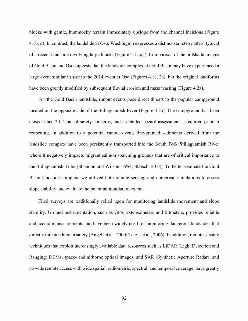
92
blocks with gentle, hummocky terrain immediately upslope from the channel incisions (Figure
4.1b, d). In contrast, the landslide at Oso, Washington expresses a distinct stairstep pattern typical
of a recent landslide involving large blocks (Figure 4.1c,e,f). Comparison of the hillshade images
of Gold Basin and Oso suggests that the landslide complex at Gold Basin may have experienced a
large event similar in size to the 2014 event at Oso (Figures 4.1c, 2a), but the original landforms
have been greatly modified by subsequent fluvial erosion and mass wasting (Figure 4.2a).
For the Gold Basin landslide, runout events pose direct threats to the popular campground
located on the opposite side of the Stillaguamish River (Figure 4.2a). The campground has been
closed since 2014 out of safety concerns, and a detailed hazard assessment is required prior to
reopening. In addition to a potential runout event, fine-grained sediments derived from the
landslide complex have been persistently transported into the South Fork Stillaguamish River
where it negatively impacts migrant salmon spawning grounds that are of critical importance to
the Stillaguamish Tribe (Shannon and Wilson, 1954; Staisch, 2018). To better evaluate the Gold
Basin landslide complex, we utilized both remote sensing and numerical simulations to assess
slope stability and evaluate the potential inundation extent.
Filed surveys are traditionally relied upon for monitoring landslide movement and slope
stability. Ground instrumentation, such as GPS, extensometers and tiltmeters, provides reliable
and accurate measurements and have been widely used for monitoring dangerous landslides that
directly threaten human safety (Angeli et al., 2000; Terzis et al., 2006). In addition, remote sensing
techniques that exploit increasingly available data resources such as LiDAR (Light Detection and
Ranging) DEMs, space- and airborne optical images, and SAR (Synthetic Aperture Radar), and
provide remote access with wide spatial, radiometric, spectral, and temporal coverage, have greatly
93
improved the efficiency of landslide detection and mapping (e.g. Fruneau et al., 1996; Squarzoni
et al., 2003; Colesanti and Wasowski, 2006; Xu et al., 2019).
Figure 4.1 Comparison between the Gold Basin landslide and the Oso slide. (a) Geographic locations of the Gold Basin landslide complex (red square) and the Oso slide (red triangle), with the annotation WA=Washington. Hillshade images of (b) Gold Basin landslide complex (red polygon) and (c) Oso slide. Cyan polylines in (b) represent stream valleys and the yellow square outlines the headscarps shown in (d). True-color images of Oso slide (e) before and (f) after the 2014 runout event. Images were obtained from Google Earth. LiDAR DEMs were accessed from the Washington State Department of Natural Resources.
However, despite multiple available data sources, remote sensing surveillance of slopes in
particular terrains and at certain times still presents challenges due to current technical limitations.
The effectiveness of utilizing SAR images for landslide studies depends on their spatial resolution,
wavelength of the SAR signal, the revisit cycle of SAR satellites, the look angle of SAR sensors,
and the motion rate of landslides (e.g. the InSAR method may not be effective for rapidly moving
94
slides), while that of LiDAR is primarily affected by available repeated acquisitions. For the free
or low-cost optical images from satellite platforms such as Landsat and Sentinel-2, coarse spatial
resolution and cloud coverage are the two key limiting factors. Consequently, a single remote
sensing device might not be adequate to detect and monitor some landslide scenarios (e.g. a small
localized collapse of a steep slope at a particular time). Nevertheless, integrating multiple remotely
sensed datasets and employing suitable interpretation methods provides a potential solution for
certain difficult cases.
In order to evaluate the potential runout and inundation extent, should a slope failure lead to a
rapidly flowing landslide and debris flow, we employed numerical modeling using the D-claw
package (George and Iverson, 2014) D-claw is a depth-averaged two-phase model that simulates
the flow dynamics based on conservation of mass and momentum, and accounting for the
important feedbacks between solid grain concentrations and the basal pore-fluid pressure that
regulate flow resistance and mobility, based in part on the theory of granular dilatancy for shearing
soils (Iverson and George, 2014). Running a D-claw model requires a hypothetical landslide basal
slip surface that defines the initial landslide volume and geometry (George and Iverson, 2014;
Iverson et al., 2015).
This investigation focuses on using multiple remote sensing datasets to monitor movement of
the Gold Basin landslide complex, which also helps constrain initial, hypothetical landslide source
geometries as an input for the D-claw simulations of runout scenarios. Due to the steep slopes and
large yet localized deformation, multiple SAR processing methods are employed to characterize
the landslide motions. D-claw simulations are subsequently performed to evaluate the potential
hazard zone. Our methodology of evaluating landslide runout hazards developed for this case study
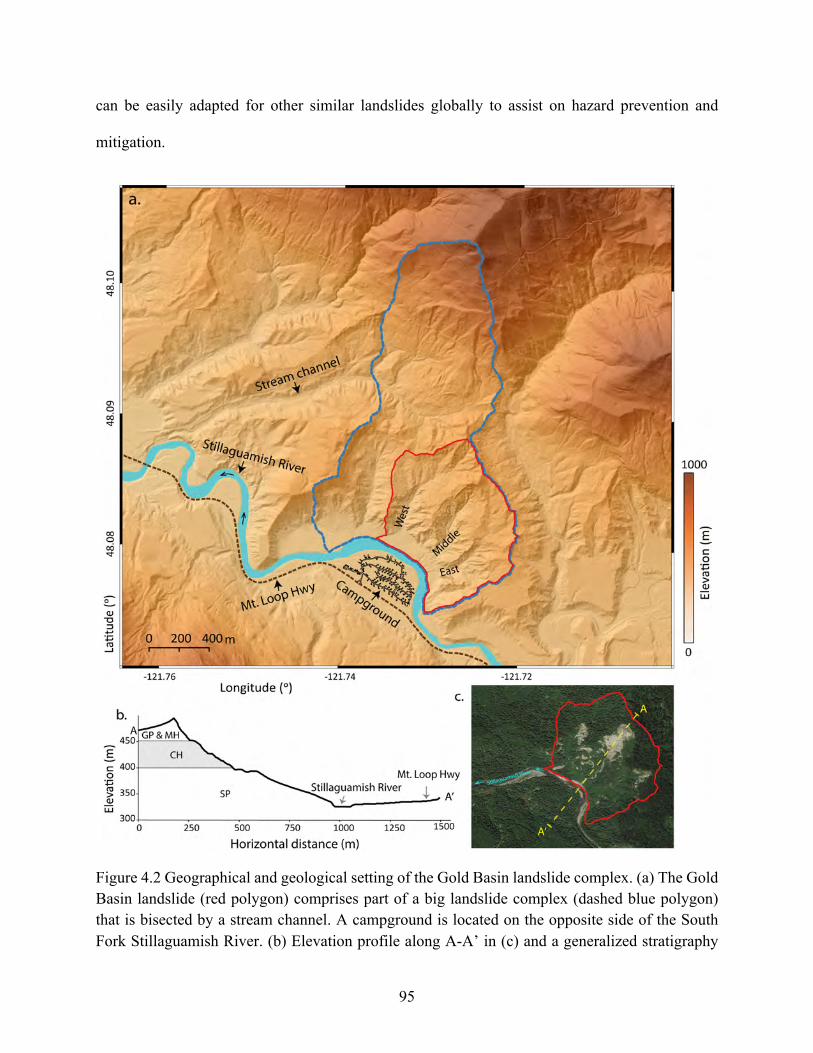
95
can be easily adapted for other similar landslides globally to assist on hazard prevention and
mitigation.
Figure 4.2 Geographical and geological setting of the Gold Basin landslide complex. (a) The Gold Basin landslide (red polygon) comprises part of a big landslide complex (dashed blue polygon) that is bisected by a stream channel. A campground is located on the opposite side of the South Fork Stillaguamish River. (b) Elevation profile along A-A’ in (c) and a generalized stratigraphy
96
obtained by McCabe (2016). Soil types were classified following the Unified Soil Classification System (USCS) with GP=poorly graded gravel, MH=silt of high plasticity and elastic silt, CH=clay of high plasticity and fat clay, and SP=poorly graded sand. (c) A true-color image of the slide obtained in July 2018 from Google Earth.
4.2 Geological Setting and History
4.2.1 Regional Setting
The Gold Basin landslide complex, located in Snohomish County, Washington (Figure
4.1a,b), lies above the South Fork of the Stillaguamish River in the Cascade Range (Figure 4.2a).
The landslide complex’s elevation ranges from 325 m to 495 m above sea level, and consists of
three small, steep tributary valleys that form three separate lobes on the north valley wall and
transport landslide debris and sediment downstream to the Stillaguamish River through valley
channels (Figure 4.1b). The valleys at Gold Basin were originally filled with recessional glacial
deposits to a substantial depth of 175 m. The river has cut through deposits (Benda and Collins,
1992; Staisch, 2018) and form steep-sided valley walls exposing the glacial stratigraphy (Miller
and Miller, 1999; Miller, 2019). Stratigraphy is vertically and laterally heterogeneous with
discontinuous lenses of silt and clay interspersed in sandy river deposits. Field observations and
lab tests indicate that there is a 52.6 m water-perching layer (400.9–453.5 m above sea level) of
silt sand clays between strata of poorly sorted gravels and sands in the stratigraphy of the middle
lobe (Figure 4.2b; McCabe, 2016).
4.2.2 Historical Landslide Activity
Three large historical runout events have been recorded at Gold Basin, though the involved
lobes varied over time. Cycles of small, localized collapses and erosion have been occurring
intermittently over many decades, followed by subsequent revegetation. The earliest recoded
landslide activity can be traced back to 1942 (Benda and Collins, 1992). The landslide source was
97
confined to the lower portions of the middle lobe and the eastern-most lobe, and the active area
was approximately a quarter of the much larger 1964 landslide. The 1964 event occurred in the
eastern-most lobe and formed a fan at the mouth of that lobe, as indicated by the exposed bare
ground in aerial images (Figure 4.3; Miller and Miller, 1999). Subsequent vegetation regrowth
eventually obscured the fan, and by 1983 the river had eroded back the toe of the eastern-most
lobe (Miller, 2019). The most recent debris flow occurred in 1996, in the middle and western-most
lobes. Debris deposits blocked the river and had shifted the channel to the south where it currently
remains. The evolution of the channel course is apparent from comparing the 1995 and 2007
images of the site (Figure 4.3).
4.3 Methodology and Data
4.3.1 Measuring Landslide Movement Using Remote Sensing
4.3.1.1 LiDAR DEM differencing
LiDAR DEMs have proven to be an effective tool for landslide detection because of their high
spatial resolution and high measurement accuracy (e.g. Hodgson et al., 2003; Roering et al., 2009).
The sub-meter-level spatial resolution and the centimeter-level absolute accuracy provide for
reliable and accurate measurements of landslide motions, ranging from localized small
displacements to large runout events. Moreover, landslide detection with LiDAR point clouds is
largely impervious to the influence of vegetation, slope angle, and ground features. However, at
the state level there is presently only limited LiDAR spatial coverage, and typically the datasets
are very sparse in terms of repeated temporal sampling. Considering the Gold Basin region for
example, LiDAR DEMs are only available for years 2005, 2006, 2013, and 2016 and lack full
spatial continuity for the project area, which is essential for differencing. Nevertheless, hillshade
98
images produced from high resolution DEMs facilitate interpretation of landforms and provide
insights into the landslide processes (Figure 4.2a). In this investigation, we applied DEM
differencing to all available LiDAR DEMs in the Gold Basin region to quantify the deformation
rates and landslide volumes from 2005 to 2016.
4.3.1.2 InSAR
InSAR (Interferometric Synthetic Aperture Radar) methods are focused on the phase
information of SAR backscattering and can optimally provide up to millimeter-level measurement
accuracy along the LOS (line of sight) direction (e.g. Hanssen, 2001). However, substantial pixel
displacements can present coherence degradation and unwrapping problems (e.g. Lu and Dzurisin,
2014). Consequently, applying InSAR to measure landslide movements with high deformation
gradients (phase difference between two adjacent pixels exceeds :/2) requires additional data
inputs or assumptions of displacement patterns (e.g. Xu et al., 2019). The long-wavelength L-band
data generally maintains better coherence in vegetated terrains and yields better interferometric
results than the shorter-wavelength C-band and X-band SAR images (Xu et al., 2019).
As LiDAR DEMs are unavailable after 2016, we processed all available SAR data from the
L-band ALOS-2 PALSAR-2, the C-band Sentinel-1A/B, and the X-band TerraSAR-X to detect
recent landslide activities between 2017 and 2019 using the InSAR method.
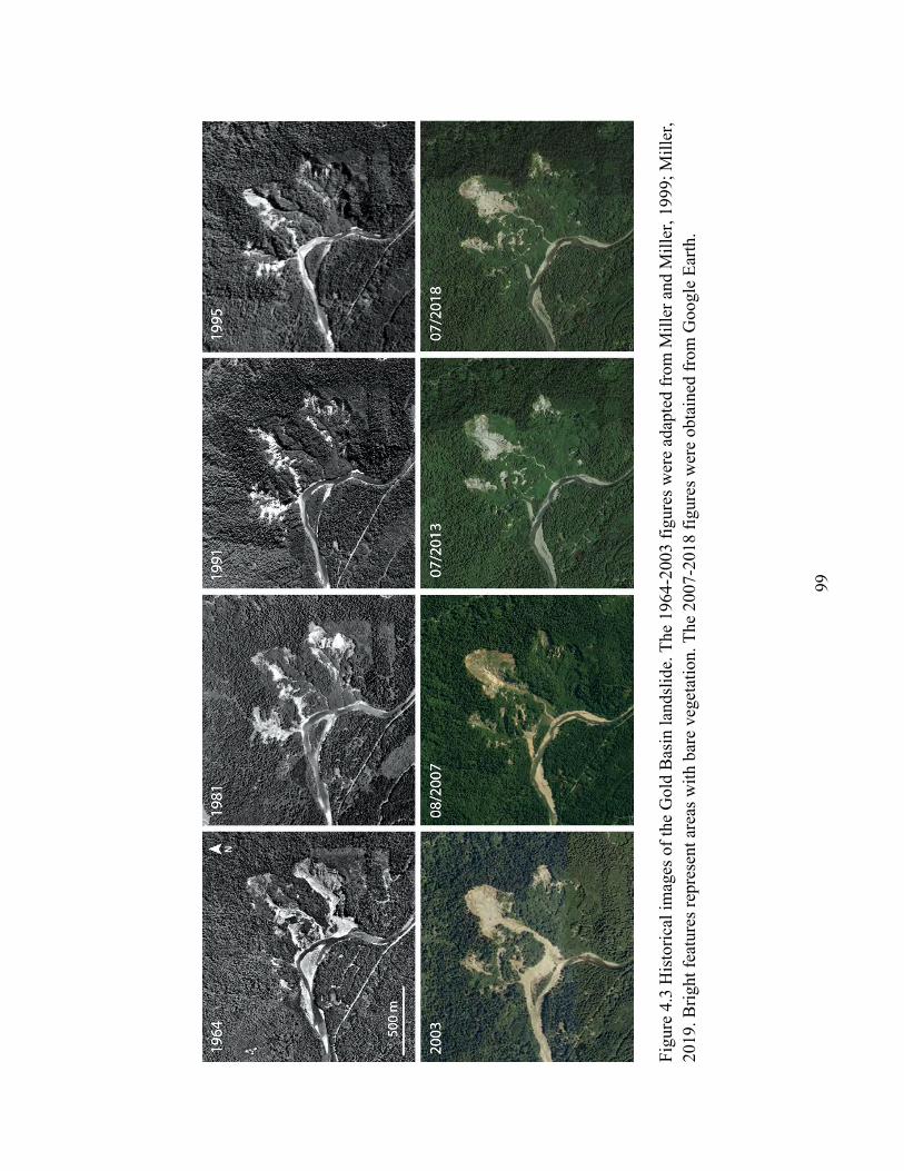
99
Figu
re 4
.3 H
isto
rical
imag
es o
f the
Gol
d B
asin
land
slid
e. T
he 1
964-
2003
figu
res w
ere
adap
ted
from
Mill
er a
nd M
iller
, 199
9; M
iller
, 20
19. B
right
feat
ures
repr
esen
t are
as w
ith b
are
vege
tatio
n. T
he 2
007-
2018
figu
res w
ere
obta
ined
from
Goo
gle
Earth
.

100
4.3.1.3 SAR intensity differencing and pixel offset tracking
SAR intensity refers to the strength of the reflected signal from ground objects. Landslide
activity that causes measurable changes of the backscattering signal can be detected by
differencing SAR intensity images (e.g. Plank et al., 2016). However, solely differencing SAR
intensity changes cannot confirm a landslide activity, as other factors, such as changes in soil
moisture and variations in forest-cover density (associated with wildfire, disease, or silvicultural
activities such as timber harvest thinning or fuel management), also cause fluctuation of
backscattering signals. An alternate approach is to track pixel offsets between two SAR intensity
images using cross correlation (e.g. Strozzi et al., 2002; Singleton et al., 2014). The offset tracking
accuracy can reach 1/20 to 1/10 pixels (Hanssen, 2001). We applied both SAR intensity
differencing and pixel offset tracking to detect recent landslide activity at Gold Basin.
First, we implemented intensity change detection methods on the high-spatial-resolution
TerraSAR-X data from Jan 2017 to March 2019 to detect the existence of highly localized
deformations. As a single-look SAR image generally contains significant speckle noises (e.g.
Hassen, 2001), we multi-looked every image with a 3×3 multilook factor and averaged five images
acquired in the same season to form one image for detecting intensity changes. Three SAR
intensity images of years 2017, 2018 and 2019 were generated by averaging SAR images acquired
between January and March in corresponding years (~ 5 images for each year), and then utilized
to calculate intensity changes.
Second, we applied the pixel offset tracking method to the same Tandem-X datasets from
2017 to 2019. Unlike the intensity change detection, pixel offset tracking can provide quantitative
measurements of landslide movement. Similarly, we averaged five SAR intensity images between
January and March of each year, before conducting offset tracking. Here we did not employ multi-
101
looking, because multi-looking would increase pixel size and consequently reduce offset-tracking
accuracy. Pixel offset tracking was carried out twice iteratively with downscaling window sizes.
A window size of 64×64 pixels was set for the first round of offset tracking, and the output was
used as the input for the second-round of offset tracking after eliminating offset anomalies. The
second round started with a smaller window size of 32×32 pixels, and the final results were
smoothed using a moving window of 2×2 pixels.
4.3.2 Runout Scenario Simulation
4.3.2.1 D-claw model
D-claw is a depth-averaged two-phase model that combines concepts of critical-state soil
mechanics, grain-flow mechanics, and fluid dynamics (Iverson and George, 2014; George and
Iverson, 2014). The model’s five balance equations describe coupled evolution of the solid volume
fraction, basal pore-fluid pressure, flow thickness, and two components of flow velocity are given
as:
"ℎ"$+"(ℎ')")
+"(ℎ*)"+
=- − -!-
/(4.14)
"(ℎ')"$
+"")(ℎ'") + 5
"")6128#ℎ"9 +
"(ℎ'*)"+
+ℎ(1 − 5)
-":$")
= ℎ8% + '/- − -!-
−;&,% + ;!,%
-(4.1<)
"(ℎ')"$
+"(ℎ'*)")
+""+(ℎ*") + 5
""+6128#ℎ"9 +
ℎ(1 − 5)-
":$"+
= ℎ8( + */- − -!-
−;&,( + ;!,(
-(4.1=)
102
"(ℎ>)"$
+"(ℎ'>)")
+"(ℎ*>)"+
= −/>-!-(4.1?)
":$"$
− -8#@'"ℎ")
+ -8#@"(ℎ')")
+ '":$")
− -8#@*"ℎ"+
+ -8#@"(ℎ*)"+
+ *":$"+
= A/ −3C)ℎ
‖(', *)*‖ tanI+ (4.1J)
where ℎ is the height normal to the bed of a virtual free surface, ' and * are the depth-averaged
flow velocities in the ) and + directions, respectively, > is the depth-averaged solid volume
fraction and :$ denotes the pore-fluid pressure at the basal boundary, 8# is the gravitational
acceleration in the bed-normal direction (i.e. K = L8% , 8( , 8#M*), 5 is the lateral pressure
coefficient, C) is the elastic compressibility, I+ is the granular dilatancy angle, the terms N& =
L;&,% , ;&,(M*
and N! = L;!,% , ;!,(M*
are the basal shear traction exerted by the solid phase and fluid
phase, respectively, and - is the depth-averaged bulk density, which is a function of the solid
volume fraction
- = -&> + (1 −>)-!(4.2)
where -& and -! are the intrinsic material densities of the solid and fluid constituencies,
respectively, which are assumed to be constant. The variable coefficient @ is given by
@ =-! + 3-4-
(4.3)
The variable A is introduced in equation 4.1e for notational convenience and is given by
A =3
2C)ℎ+8#-!L- − -!M
4-(4.4)
103
/ is the depth-averaged granular dilation rate, equal to the depth integral of the divergence of the
solid-phase velocity field and is proportional to the difference between basal pore-fluid pressure
and hydrostatic pressure
/ = −2OℎPL:$ − :!8#ℎM(4.5)
where O is the hydraulic permeability and P is the pore-fluid viscosity.
The dilatancy angle I+ depending on > is defined as
tanI = > −>-. (4.6)
where
>-. =>)/011 + √T
(4.7)
Here >)/01 is the critical-state solid volume fraction commonly employed in soil mechanics (i.e.
the quasi-static equilibrium solid volume fraction such that there is no change in > during
shearing, with V- constant). The quantity T is a dimensionless state parameter defined as
T =PW
-&W"Y" + V-′
(4.8)
where W = 2‖', *‖* is an estimate of the depth-averaged shear rate, V- is the effective stress, and
Y is a length scale associated with grain collisions (Iverson and George, 2014). In the USGS
plume experiments, >)/01 ranges from 0.56 to 0.64, and δ was set as 1mm.
The D-claw model incorporates the theory of soil dilatancy in order to mediate the feedback
effects of soil-shearing and fluid-pressure-dependent mobility and resistance. Adjustable
parameters in the model are based on well-established and measurable material quantities (e.g.
initial porosity, hydraulic permeability, solid-matrix elastic compressibility, etc.) In lieu of site-
104
specific studies of these parameters, they are constrained to reasonable bounds by sediment tests
of materials in analogous studies or geologically similar regions (see e.g. Iverson et al., 2010,
2015).
The predicted debris-flow behavior is influenced by several non-dimensional quantities
identified by Iverson and George (2014) and depends on landslide initial conditions and evolving
material properties. These quantities include the difference between the initial sediment porosity
and an evolving equilibrium porosity, >2 −>-.3. The evolving equilibrium volume fraction
>-.3, depends on the state of flow variables and an initial, or critical equilibrium >)/01, which
represents the quasi-static equilibrium volume fraction prior to motion. The sign of >2 −>-.3
determines whether soils are in a contractive state in which initial shearing leads to increased
mobility, or a dilative state in which shearing decreases mobility. The two alternative states of the
material lead to either positive feedbacks and flow acceleration or negative feedbacks and flow
stabilization and deposition. For characterizing hazards that may result from high-mobility
landslides, the former, generally contractive initial state of debris is assumed.
4.3.2.2 Log-spiral basal surfaces
To simulate hypothetical runout scenarios using the D-claw package, landslide basal slip
surfaces are required. In lieu of additional site-specific data, basal surfaces are typically assumed
to have longitudinal transects that conform to a logarithmic-spiral shape, a commonly assumed
feature of idealized landslide scarps. For a homogeneous slope and assuming a visco-elastic
rheology of shearing soils, the Mohr-Coulomb yield criterion leads to a logarithmic-spiral failure
surface (Baker and Garber, 1978; Chen, 2013). In the polar coordinate, the log-spiral is described
as
\ = \2J4 5678(4.9)
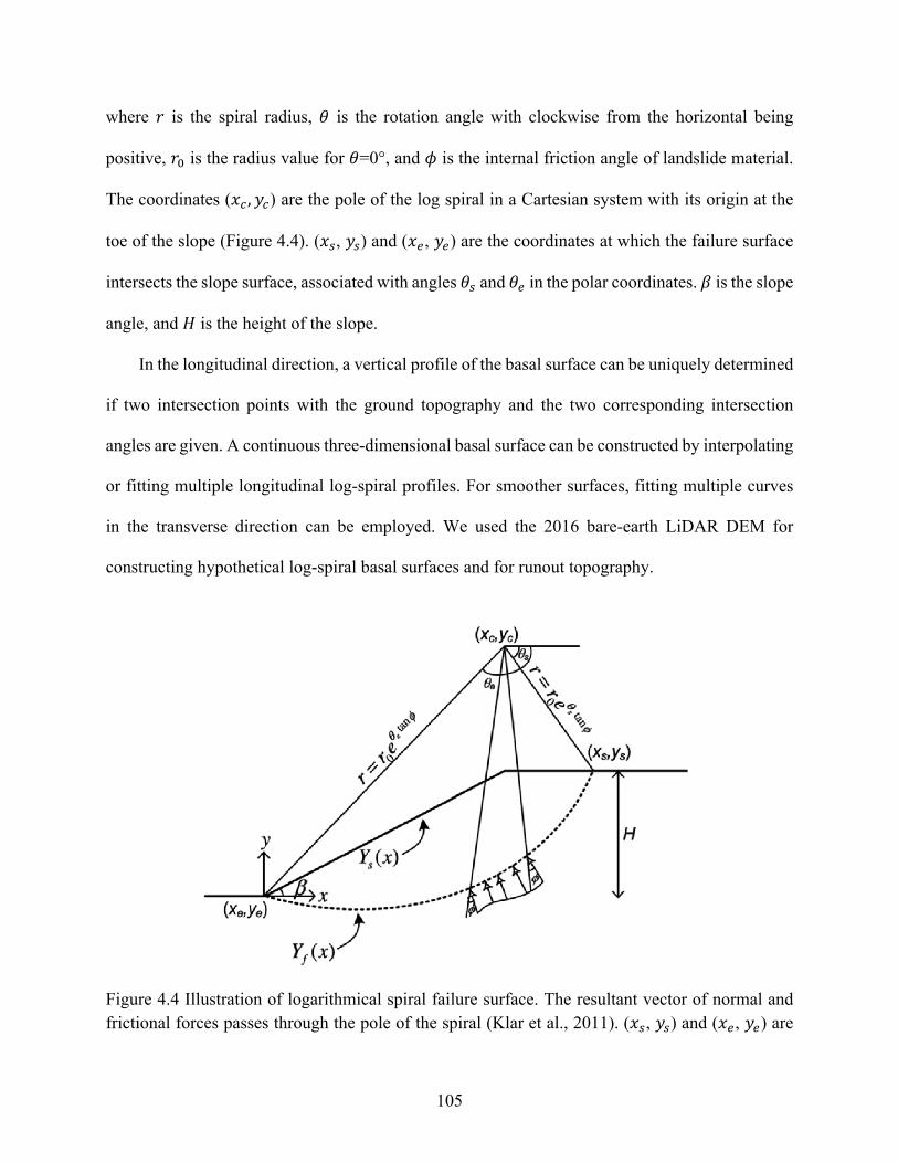
105
where \ is the spiral radius, ^ is the rotation angle with clockwise from the horizontal being
positive, \2 is the radius value for ^=0°, and _ is the internal friction angle of landslide material.
The coordinates ()) , +)) are the pole of the log spiral in a Cartesian system with its origin at the
toe of the slope (Figure 4.4). ()&, +&) and ()-, +-) are the coordinates at which the failure surface
intersects the slope surface, associated with angles & and - in the polar coordinates. is the slope
angle, and a is the height of the slope.
In the longitudinal direction, a vertical profile of the basal surface can be uniquely determined
if two intersection points with the ground topography and the two corresponding intersection
angles are given. A continuous three-dimensional basal surface can be constructed by interpolating
or fitting multiple longitudinal log-spiral profiles. For smoother surfaces, fitting multiple curves
in the transverse direction can be employed. We used the 2016 bare-earth LiDAR DEM for
constructing hypothetical log-spiral basal surfaces and for runout topography.
Figure 4.4 Illustration of logarithmical spiral failure surface. The resultant vector of normal and frictional forces passes through the pole of the spiral (Klar et al., 2011). ()&, +&) and ()-, +-) are
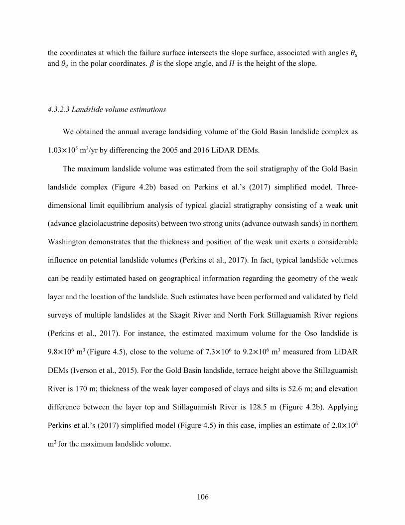
106
the coordinates at which the failure surface intersects the slope surface, associated with angles & and - in the polar coordinates. ` is the slope angle, and a is the height of the slope.
4.3.2.3 Landslide volume estimations
We obtained the annual average landsiding volume of the Gold Basin landslide complex as
1.03×10⁵ m3/yr by differencing the 2005 and 2016 LiDAR DEMs.
The maximum landslide volume was estimated from the soil stratigraphy of the Gold Basin
landslide complex (Figure 4.2b) based on Perkins et al.’s (2017) simplified model. Three-
dimensional limit equilibrium analysis of typical glacial stratigraphy consisting of a weak unit
(advance glaciolacustrine deposits) between two strong units (advance outwash sands) in northern
Washington demonstrates that the thickness and position of the weak unit exerts a considerable
influence on potential landslide volumes (Perkins et al., 2017). In fact, typical landslide volumes
can be readily estimated based on geographical information regarding the geometry of the weak
layer and the location of the landslide. Such estimates have been performed and validated by field
surveys of multiple landslides at the Skagit River and North Fork Stillaguamish River regions
(Perkins et al., 2017). For instance, the estimated maximum volume for the Oso landslide is
9.8×10⁶ m3 (Figure 4.5), close to the volume of 7.3×10⁶ to 9.2×10⁶ m3 measured from LiDAR
DEMs (Iverson et al., 2015). For the Gold Basin landslide, terrace height above the Stillaguamish
River is 170 m; thickness of the weak layer composed of clays and silts is 52.6 m; and elevation
difference between the layer top and Stillaguamish River is 128.5 m (Figure 4.2b). Applying
Perkins et al.’s (2017) simplified model (Figure 4.5) in this case, implies an estimate of 2.0×10⁶
m3 for the maximum landslide volume.
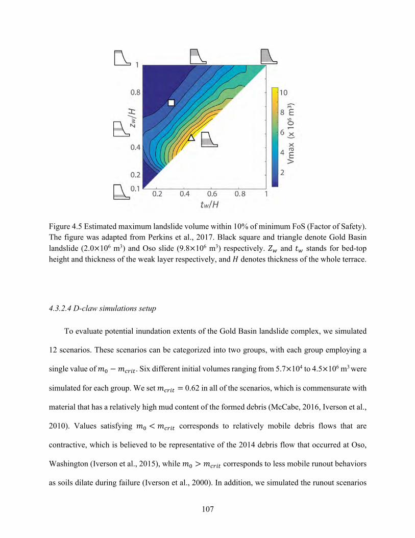
107
Figure 4.5 Estimated maximum landslide volume within 10% of minimum FoS (Factor of Safety). The figure was adapted from Perkins et al., 2017. Black square and triangle denote Gold Basin landslide (2.0×10⁶ m3) and Oso slide (9.8×10⁶ m3) respectively. b9 and $9 stands for bed-top height and thickness of the weak layer respectively, and a denotes thickness of the whole terrace.
4.3.2.4 D-claw simulations setup
To evaluate potential inundation extents of the Gold Basin landslide complex, we simulated
12 scenarios. These scenarios can be categorized into two groups, with each group employing a
single value of >2 −>)/01. Six different initial volumes ranging from 5.7×10⁴ to 4.5×10⁶ m3 were
simulated for each group. We set >)/01 =0.62 in all of the scenarios, which is commensurate with
material that has a relatively high mud content of the formed debris (McCabe, 2016, Iverson et al.,
2010). Values satisfying >2 < >)/01 corresponds to relatively mobile debris flows that are
contractive, which is believed to be representative of the 2014 debris flow that occurred at Oso,
Washington (Iverson et al., 2015), while >2 > >)/01 corresponds to less mobile runout behaviors
as soils dilate during failure (Iverson et al., 2000). In addition, we simulated the runout scenarios
108
with a flowing river presented at the landslide toe for the case of landslide volume e = 2.1×10⁶
m3. The water depth was set as two meters for the entire river segment near the landslide.
4.4 Results
4.4.1 Remote Sensing of Landslide Activity
4.4.1.1 LiDAR DEM differencing
Differencing of 2005 and 2016 DEMs reveals that substantial localized deformation of the
western-most and middle lobes occurred, with a maximum displacement of ~ 30 meters, while
only slight deformation was observed at the eastern-most lobe (Figure 4.6a). From 2013 to 2016,
some localized yet substantial collapses (about 20 m in displacement) appeared at the head scarp
of the middle lobe (Figure 4.6b). Similar substantial deformation was also captured by terrestrial
LiDAR from July 2015 to January 2016 (McCabe, 2016). As the overlap region of the 2013 and
2016 DEMs only covers the head section of the slope, it is not clear whether localized movements
also occurred at the lower sections from 2013 to 2016. Nearly no deformation occurred between
June 2005 and March 2006.
4.4.1.2 InSAR
We processed all available SAR acquisitions from ALOS-2 PALSAR-2, Sentinel-1A/B, and
TerraSAR-X. However, only the L-band ALOS-2 imagery produced useful interferograms for
identifying ground deformation due to severe coherence loss of the shorter-wavelength C-band
Sentinel-1A/B and X-band TerraSAR-X images. Five active landslides nearby Gold Basin were
detected by an ALOS-2 interferogram spanning from 2016 to 2017 (Figure 4.7), yet deformation
signals at the Gold Basin landslide complex were not distinguishable due to poor coherence there.
The most likely reason is that the relatively coarse spatial resolution (~10 m) and look angle (~35˚)
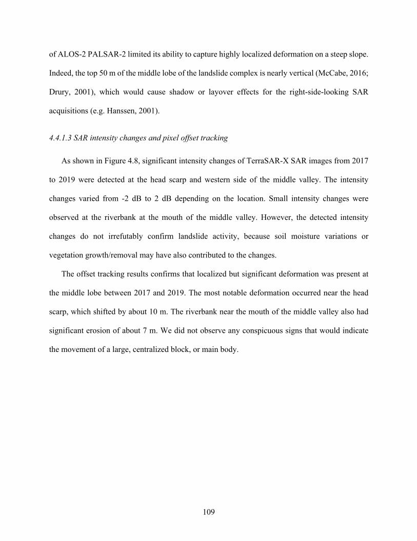
109
of ALOS-2 PALSAR-2 limited its ability to capture highly localized deformation on a steep slope.
Indeed, the top 50 m of the middle lobe of the landslide complex is nearly vertical (McCabe, 2016;
Drury, 2001), which would cause shadow or layover effects for the right-side-looking SAR
acquisitions (e.g. Hanssen, 2001).
4.4.1.3 SAR intensity changes and pixel offset tracking
As shown in Figure 4.8, significant intensity changes of TerraSAR-X SAR images from 2017
to 2019 were detected at the head scarp and western side of the middle valley. The intensity
changes varied from -2 dB to 2 dB depending on the location. Small intensity changes were
observed at the riverbank at the mouth of the middle valley. However, the detected intensity
changes do not irrefutably confirm landslide activity, because soil moisture variations or
vegetation growth/removal may have also contributed to the changes.
The offset tracking results confirms that localized but significant deformation was present at
the middle lobe between 2017 and 2019. The most notable deformation occurred near the head
scarp, which shifted by about 10 m. The riverbank near the mouth of the middle valley also had
significant erosion of about 7 m. We did not observe any conspicuous signs that would indicate
the movement of a large, centralized block, or main body.
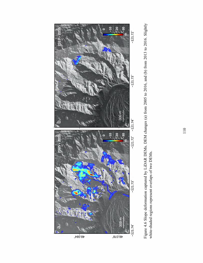
110
Fig
ure
4.6
Slo
pe d
efor
mat
ion
capt
ured
by
LiD
AR
DE
Ms.
DE
M c
hang
es (
a) f
rom
200
5 to
201
6, a
nd (
b) f
rom
201
3 to
201
6. S
ligh
tly
whi
te-s
hade
d re
gion
s re
pres
ent o
verl
aps
of tw
o D
EM
s.
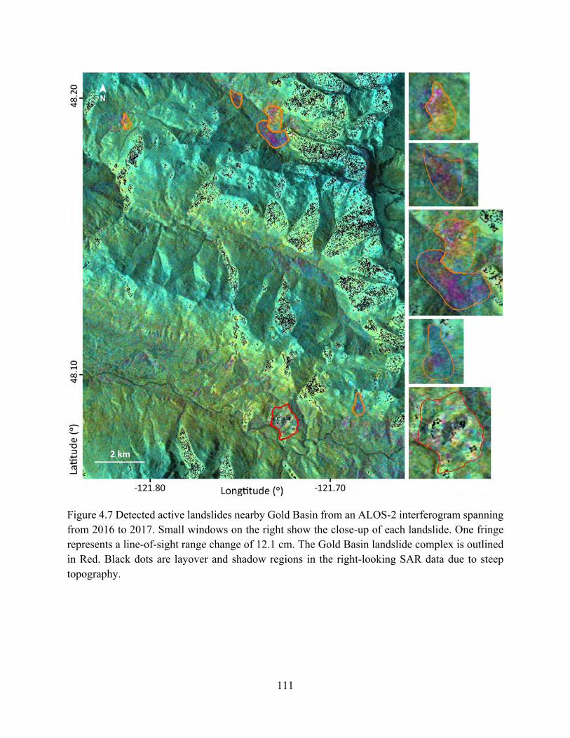
111
Figure 4.7 Detected active landslides nearby Gold Basin from an ALOS-2 interferogram spanning from 2016 to 2017. Small windows on the right show the close-up of each landslide. One fringe represents a line-of-sight range change of 12.1 cm. The Gold Basin landslide complex is outlined in Red. Black dots are layover and shadow regions in the right-looking SAR data due to steep topography.
112
Figu
re 4
.8 In
tens
ity c
hang
es a
nd tr
acke
d di
spla
cem
ents
of T
erra
SAR
-X im
ages
span
ning
201
7–20
18 (l
eft c
olum
n), 2
018–
2019
(mid
dle
colu
mn)
, and
201
7–20
19 (r
ight
col
umn)
.
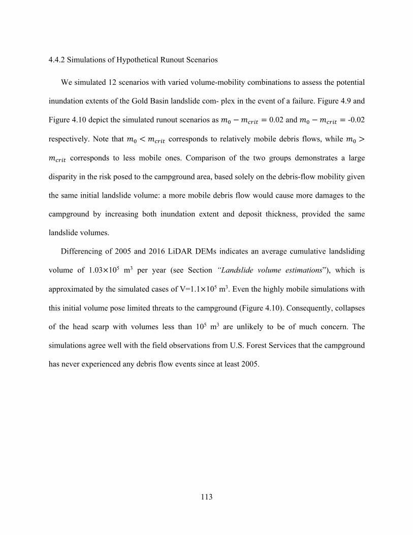
113
4.4.2 Simulations of Hypothetical Runout Scenarios
We simulated 12 scenarios with varied volume-mobility combinations to assess the potential
inundation extents of the Gold Basin landslide com- plex in the event of a failure. Figure 4.9 and
Figure 4.10 depict the simulated runout scenarios as !! −!"#$% = 0.02 and !! −!"#$% = -0.02
respectively. Note that !! < !"#$% corresponds to relatively mobile debris flows, while !! >
!"#$% corresponds to less mobile ones. Comparison of the two groups demonstrates a large
disparity in the risk posed to the campground area, based solely on the debris-flow mobility given
the same initial landslide volume: a more mobile debris flow would cause more damages to the
campground by increasing both inundation extent and deposit thickness, provided the same
landslide volumes.
Differencing of 2005 and 2016 LiDAR DEMs indicates an average cumulative landsliding
volume of 1.03×10⁵ m3 per year (see Section “Landslide volume estimations”), which is
approximated by the simulated cases of V=1.1×10⁵ m3. Even the highly mobile simulations with
this initial volume pose limited threats to the campground (Figure 4.10). Consequently, collapses
of the head scarp with volumes less than 105 m3 are unlikely to be of much concern. The
simulations agree well with the field observations from U.S. Forest Services that the campground
has never experienced any debris flow events since at least 2005.
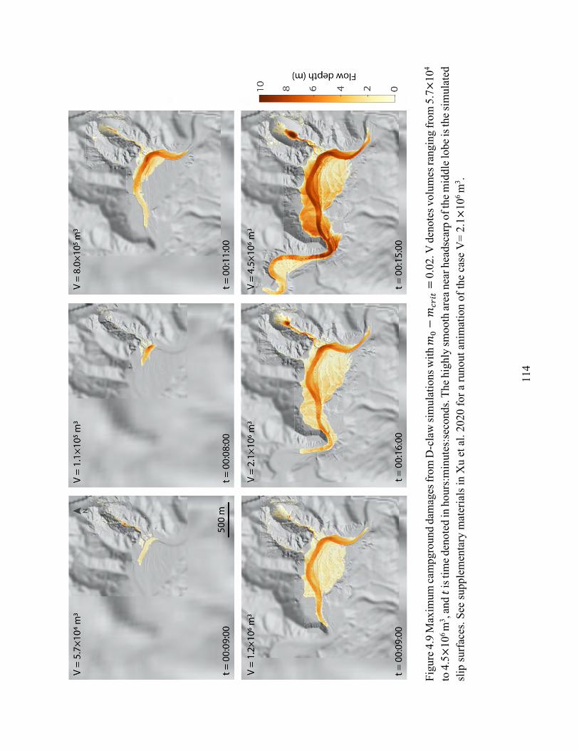
114
Figu
re 4
.9 M
axim
um ca
mpg
roun
d da
mag
es fr
om D
-cla
w si
mul
atio
ns w
ith !
!−! "
#$%=
0.02
. V d
enot
es v
olum
es ra
ngin
g fr
om 5
.7×1
04
to 4
.5×1
06 m
3 , an
d % i
s tim
e den
oted
in h
ours
:min
utes
:sec
onds
. The
hig
hly
smoo
th ar
ea n
ear h
eads
carp
of t
he m
iddl
e lob
e is t
he si
mul
ated
sl
ip su
rfac
es. S
ee su
pple
men
tary
mat
eria
ls in
Xu
et a
l. 20
20 fo
r a ru
nout
ani
mat
ion
of th
e ca
se V
= 2.
1×10
6 m
3 .
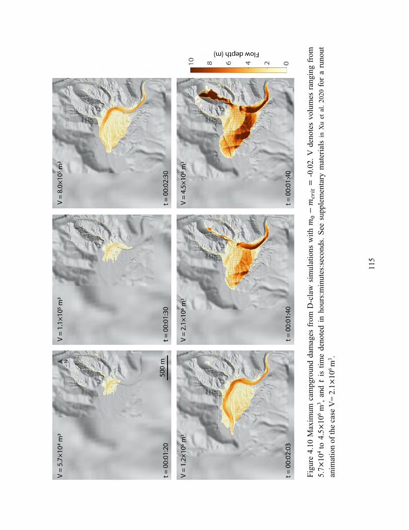
115
Figu
re 4
.10
Max
imum
cam
pgro
und
dam
ages
fro
m D
-cla
w s
imul
atio
ns w
ith !
!−! "
#$%=
-0.0
2. V
den
otes
vol
umes
ran
ging
fro
m
5.7×
104
to 4
.5×1
06 m
3 , an
d % i
s tim
e de
note
d in
hou
rs:m
inut
es:s
econ
ds. S
ee s
uppl
emen
tary
mat
eria
ls in
Xu
et a
l. 20
20 fo
r a
runo
ut
anim
atio
n of
the
case
V=
2.1×
106 m
3 .
116
However, once landslide volumes exceed 106 m3, the simulated debris flows run over the entire
campground under both mobility assumptions. As expected, larger volumes tend to increase the
runout extent as well as the thickness of deposits on the campground. The estimated maximum
landslide volume of 2.0×10⁶ m3 (see Section “Landslide volume estimations”) is most closely
represented by our simulations with V= 2.1×10⁶ m3. As shown in Figure 4.9 and Figure 4.10, our
simulations with initial volumes of V=2.1×10⁶ m3 produce debris flows which invariably inundate
the entire campground, regardless of their simulated mobility (see supplementary materials in Xu
et al. 2020 for runout animations). The highly mobile debris flow with this initial volume crosses
the campground with an 8 m high flow front. The simulations also suggest that camp sites near the
mouth of the middle valley are the most vulnerable to potential runout events.
4.4.3 Simulations of Interactions with the Stillaguamish River
In order to evaluate how the Stillaguamish River located at the landslide toe could affect the
mobility and inundation hazards of the landslide-initiated debris flow upon a catastrophic failure,
we added a flowing river at the landslide toe and simulated corresponding runout scenarios for
both the dilative and contractive cases with landslide volume fixed at 2.1×10⁶ m3. As depicted in
Figure 4.11, the simulated results show that clearly observable debris flow fronts which are
primarily comprised of water (solid fraction ≈ 0) are generated when the landslide-initiated debris
flows move downslope and hit the Stillaguamish River for both the dilative and contractive cases.
Such scenarios can be explained by the horizontal momentum exchange between the running
debris flow front and the waterbody. However, adding the river leads to similar inundation extents
in comparison to cases without the river. Potentially, the Stillaguamish River increases the debris
volume, but such volume growth (~ 6×10⁴ m3) remains relatively small compared to the landslide
source volume (2.1×10⁶ m3) and therefore does not enlarge the inundation area considerably.
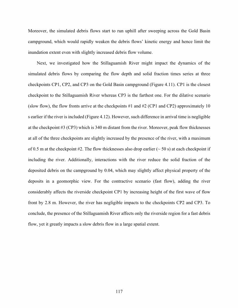
117
Moreover, the simulated debris flows start to run uphill after sweeping across the Gold Basin
campground, which would rapidly weaken the debris flows’ kinetic energy and hence limit the
inundation extent even with slightly increased debris flow volume.
Next, we investigated how the Stillaguamish River might impact the dynamics of the
simulated debris flows by comparing the flow depth and solid fraction times series at three
checkpoints CP1, CP2, and CP3 on the Gold Basin campground (Figure 4.11). CP1 is the closest
checkpoint to the Stillaguamish River whereas CP3 is the farthest one. For the dilative scenario
(slow flow), the flow fronts arrive at the checkpoints #1 and #2 (CP1 and CP2) approximately 10
s earlier if the river is included (Figure 4.12). However, such difference in arrival time is negligible
at the checkpoint #3 (CP3) which is 340 m distant from the river. Moreover, peak flow thicknesses
at all of the three checkpoints are slightly increased by the presence of the river, with a maximum
of 0.5 m at the checkpoint #2. The flow thicknesses also drop earlier (~ 50 s) at each checkpoint if
including the river. Additionally, interactions with the river reduce the solid fraction of the
deposited debris on the campground by 0.04, which may slightly affect physical property of the
deposits in a geomorphic view. For the contractive scenario (fast flow), adding the river
considerably affects the riverside checkpoint CP1 by increasing height of the first wave of flow
front by 2.8 m. However, the river has negligible impacts to the checkpoints CP2 and CP3. To
conclude, the presence of the Stillaguamish River affects only the riverside region for a fast debris
flow, yet it greatly impacts a slow debris flow in a large spatial extent.
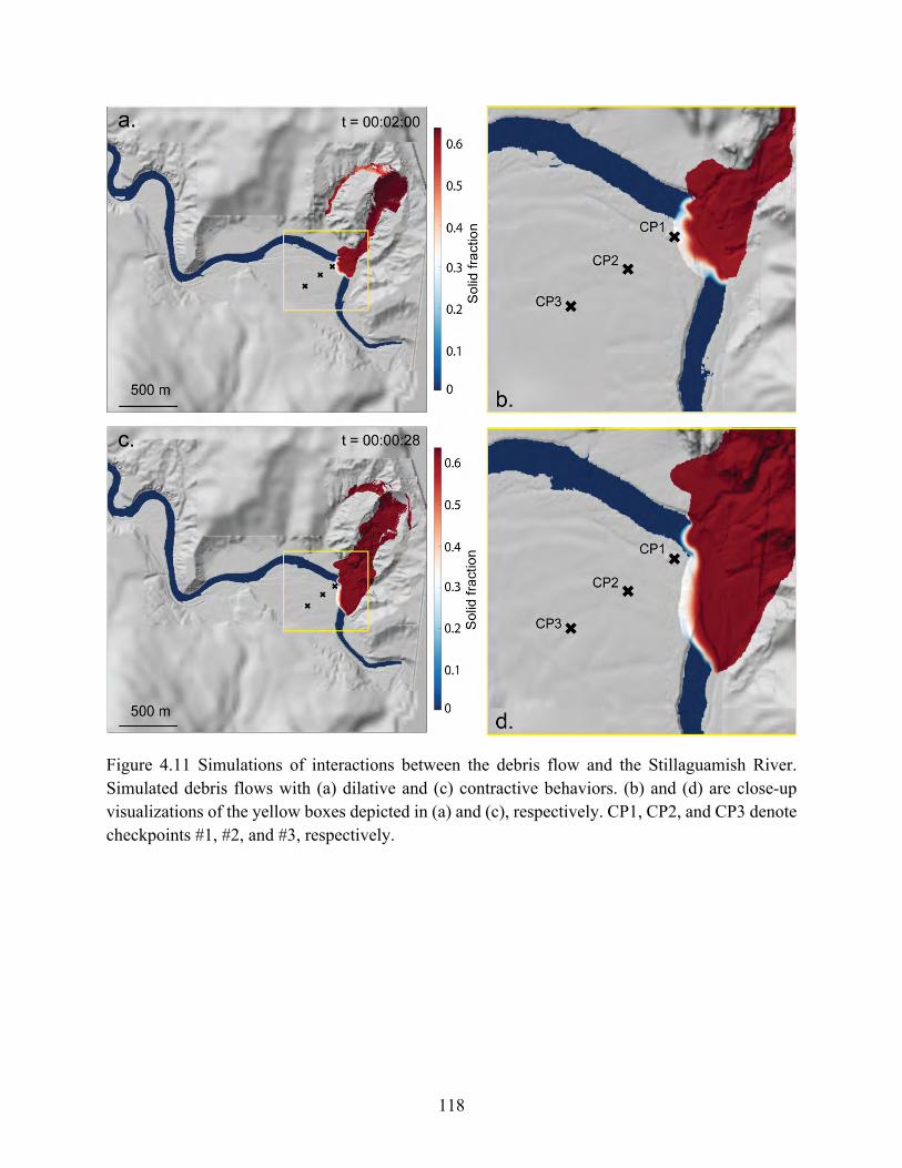
118
Figure 4.11 Simulations of interactions between the debris flow and the Stillaguamish River. Simulated debris flows with (a) dilative and (c) contractive behaviors. (b) and (d) are close-up visualizations of the yellow boxes depicted in (a) and (c), respectively. CP1, CP2, and CP3 denote checkpoints #1, #2, and #3, respectively.
119
Figure 4.12 Impacts of the river on landslide runout at different geographical locations. Geographical locations of the checkpoints #1, #2, and #3 are depicted in Figure 4.11. The first and the second rows of the figure show the evolution of flow depth and solid fraction with time for the simulated dilative flow at the checkpoints #1, #2, and #3, respectively. The third and the fourth rows show the simulations for the contractive flow.
120
4.5 Discussion
Remotely sensed data such as LiDAR DEMs and SAR provide a means for monitoring
landslide motion, at a large scale, in an efficient and cost-effective manner. However, these
methods may also present technical and practical challenges for particular difficult cases. For
instance, available LiDAR DEMs are typically temporally sparse, while the side-looking angle
and spatial resolution of SAR data limit their effectiveness for small landslides in steep or heavily
vegetated areas.
Different SAR datasets have varied advantages and disadvantages in terms of landslide
mapping. For instance, the L-band ALOS and ALOS-2 SAR sensors have great vegetation
penetration but temporally sparse acquisitions. The Sentinel-1A/B datasets provide temporally
dense sampling yet coarse resolution in azimuth direction (Xu et al., 2019). The TerraSAR-X
images have high spatial resolution but poor vegetation-penetrating capability. While using phase
information through InSAR provides the best displacement measurement accuracy, it has limited
applicability to cases with severe coherence loss. Such decorrelation might be induced by large
displacement, long spatial/temporal baselines, or ground feature changes. In contrast, offset
tracking of SAR intensity images is more tolerant to large deformation and temporal/spatial
baselines despite of the lower accuracy of 1/20 – 1/10 pixels (Hanssen, 2001). Overall, by
combining multiple sources of SAR datasets and employing optimal data processing strategies, we
have found that it is possible to maximally harness their combined attributes for landslide
monitoring.
LiDAR DEMs are able to provide reliable measurements of landslide activity with small spatial
extent, such as headscarp collapses of the Gold Basin landslide complex, but the high cost of
repeated LiDAR acquisitions and the low sensitivity to slow-moving slides comprise its primary
121
disadvantages. Nevertheless, we have shown that the challenges with individual remote sensing
technologies can largely be overcome through the simultaneous use of multiple data sources and
comprehensive data corroboration.
Modeling of landslide dynamics and inundation given an initial mass failure still presents
challenges as well, largely resulting from uncertainties about site-specific subsurface conditions
and material properties. However, by considering a range of possibilities, inundation bounds can
be approximated to a reasonable degree of certainty, at least for general hazard awareness and
effective mitigation strategies.
4.6 Conclusions
Applying complementary remote sensing data including LiDAR DEMs and SAR images to
surveil stability of the Gold Basin landslide demonstrates that only substantial and localized
displacements have occurred at the Gold Basin area between 2005 and 2019. The middle lobe has
been the most active, while the eastern-most lobe has been primarily stable during this period. The
head scarp of the middle lobe underwent a maximum displacement of approximately 40 m during
the past decade, and the western-most lobe has also experienced displacements of about 20 m at
the head scarp. Significant erosion was observed at the riverbank near the middle valley after 2017.
Average cumulative landsliding volume of the Gold basin landslide complex is 1.03×10⁵ m3 per
year. Nevertheless, from 2005 to 2019 there is no evidence indicating movement of a large central
block or single deep-seated landslide body.
Our practice of interpreting SAR with multiple approaches demonstrates that offset tracking
of high-resolution SAR is an effective alternate approach to detect landslide activity if InSAR
cannot yield reasonable results due to coherence loss induced by vegetation or steep slope angles.
122
D-claw runout simulations with multiple landslide volumes and varied runout behaviors shows
that small collapses of the head scarp with volumes less than 105 cubic meters will most likely
pose a low threat to the campground, while severely hazardous runout might occur if the initial
slide is over 106 m3. The estimated maximum volume of the Gold Basin landslide is 2.0×10⁶ m3,
indicating a significant hazard to the nearby campground should slope failure induce a mobile
landslide. The runout potential of such a landslide would depend on the landslide mobility, which
is dependent on material parameters that are difficult to constrain due to uncertainties about the
subsurface conditions. Nevertheless, flow simulations provide evidence about the range of possible
outcomes and inform hazard mitigation. In addition, our simulations demonstrate that interactions
between debris flow and waterbodies may impact the flow dynamics significantly depending on
the flow speed, waterbody volume, and the topographical settings.
In this investigation, we have proven the possibility of using remotely sensed data to measure
deformations occurred on a difficult terrain by integrating multiple data sources and
comprehensive data processing strategies. Furthermore, we have presented a means of evaluating
runout hazards of a landslide by employing the numerical model D-claw. Most importantly, these
methods developed for this case study can be easily adapted for other similar landslides globally
to assist on landslide hazards prevention and mitigation.
123
ACKNOWLEDGEMENTS
ALOS PALSAR-2 data are copyrighted by JAXA and provided under JAXA 6th Research
Announcement (3114) and JAXA 2nd Research Announcement on the Earth Observations
(ER2A2N100). This project was financially supported by NASA Interdisciplinary Research (IDS)
in Earth Science Program (80NSSC17K0022), U.S. Forest Service (16-CR-11062761-035), and
the Shuler-Foscue Endowment at Southern Methodist University.
124
REFERENCES
Angeli, M. G., Pasuto, A., and Silvano, S. (2000). A critical review of landslide monitoring experiences. Engineering Geology, 55(3), 133-147.
Baker, R., and Garber, M. (1978). Theoretical analysis of the stability of slopes. Geotechnique, 28(4), 395-411.
Benda, L., and Collins, B. (1992) Slope Stability Investigation of the Crown Pacific Property in the South Fork of the Stillaguamish River Basin, unpublished report, 37
Chen, W. F. (Ed.). (2013). Limit analysis and soil plasticity. Elsevier.
Colesanti, C., and Wasowski, J. (2006). Investigating landslides with space-borne Synthetic Aperture Radar (SAR) interferometry. Engineering geology, 88(3-4), 173-199.
Drury, A. T. (2001) Gold Basin Landslide Remediation Feasibility Study, Alternatives development and analysis, and preliminary project designs, RM 48, SF Stillaguamish River, Prepared for The Stillaguamish Tribe of Indians, 45
Fruneau, B., Achache, J., and Delacourt, C. (1996). Observation and modelling of the Saint-Etienne-de-Tinée landslide using SAR interferometry. Tectonophysics, 265(3-4), 181-190.
George, D. L., and Iverson, R. M. (2014). A depth-averaged debris-flow model that includes the effects of evolving dilatancy. II. Numerical predictions and experimental tests. Proceedings of the Royal Society A: Mathematical, Physical and Engineering Sciences, 470(2170), 20130820.
Hanssen, R. F. (2001). Radar interferometry: data interpretation and error analysis (Vol. 2). Springer Science and Business Media.
Hodgson, M. E., Jensen, J. R., Schmidt, L., Schill, S., and Davis, B. (2003). An evaluation of LIDAR-and IFSAR-derived digital elevation models in leaf-on conditions with USGS Level 1 and Level 2 DEMs. Remote sensing of environment, 84(2), 295-308.
Iverson, R. M., and George, D. L. (2014). A depth-averaged debris-flow model that includes the effects of evolving dilatancy. I. Physical basis. Proceedings of the Royal Society A: Mathematical, Physical and Engineering Sciences, 470(2170), 20130819.
125
Iverson, R. M., George, D. L., Allstadt, K., Reid, M. E., Collins, B. D., Vallance, J. W., ... and Bower, J. B. (2015). Landslide mobility and hazards: implications of the 2014 Oso disaster. Earth and Planetary Science Letters, 412, 197-208.
Iverson, R. M., Logan, M., LaHusen, R. G., and Berti, M. (2010). The perfect debris flow? Aggregated results from 28 large‐scale experiments. Journal of Geophysical Research: Earth Surface, 115(F3).
Iverson, R. M., Reid, M. E., Iverson, N. R., LaHusen, R. G., Logan, M., Mann, J. E., and Brien, D. L. (2000). Acute sensitivity of landslide rates to initial soil porosity. science, 290(5491), 513-516.
Lu, Z., and Dzurisin, D. (2014) InSAR Imaging of Aleutian Volcanoes: Monitoring a Volcanic Arc from Space: Springer Praxis Books, Geophysical Sciences, ISBN 978-3-642-00347-9, Springer, 390.
McCabe, C. (2016). Using Terrestrial LiDAR to Monitor Erosion within the Gold Basin Landslide Complex, Verlot, WA.
Miller, D. J. (2019) Gold Basin and Steelhead Haven: Landslides on the Stillaguamish, 37.
Miller, D. J., and Miller, L. R. (1999) Hazel/Gold Basin Landslides: Geomorphic Review Draft Report: M2 Environmental Services on behalf of the US Army Corps of Engineers, 26.
Perkins, J. P., Reid, M. E., and Schmidt, K. M. (2017). Control of landslide volume and hazard by glacial stratigraphic architecture, northwest Washington State, USA. Geology, 45(12), 1139-1142.
Plank, S., Twele, A., and Martinis, S. (2016). Landslide mapping in vegetated areas using change detection based on optical and polarimetric SAR data. Remote Sensing, 8(4), 307.
Roering, J. J., Stimely, L. L., Mackey, B. H., and Schmidt, D. A. (2009). Using DInSAR, airborne LiDAR, and archival air photos to quantify landsliding and sediment transport. Geophysical Research Letters, 36(19).
Shannon Wilson Engineers (1954) Report on slide on South Fork Stillaguamish River at Gold Basin Forest Camp, to the State of Washington Departments of Fisheries, 14.
Singleton, A., Li, Z., Hoey, T., and Muller, J. P. (2014). Evaluating sub-pixel offset techniques as an alternative to D-InSAR for monitoring episodic landslide movements in vegetated terrain. Remote Sensing of Environment, 147, 133-144.
Squarzoni, C., Delacourt, C., and Allemand, P. (2003). Nine years of spatial and temporal evolution of the La Valette landslide observed by SAR interferometry. Engineering Geology, 68(1-2), 53-66.
Staish, L. M. (2018). Bedrock Mapping and Seismic Hazard Assessment at Gold Basin Landslide, Washington. US Department of the Interior, US Geological Survey.
126
Strozzi, T., Luckman, A., Murray, T., Wegmuller, U., and Werner, C. L. (2002). Glacier motion estimation using SAR offset-tracking procedures. IEEE Transactions on Geoscience and Remote Sensing, 40(11), 2384-2391.
Terzis, A., Anandarajah, A., Moore, K., and Wang, I. J. (2006, April). Slip surface localization in wireless sensor networks for landslide prediction. In 2006 5th International Conference on Information Processing in Sensor Networks (pp. 109-116). IEEE.
Wartman, J., Montgomery, D. R., Anderson, S. A., Keaton, J. R., Benoît, J., dela Chapelle, J., and Gilbert, R. (2016). The 22 March 2014 Oso landslide, Washington, USA. Geomorphology, 253, 275-288.
Xu, Y., George, D. L., Kim, J., Lu, Z., Riley, M., Griffin, T., and de la Fuente, J. (2020). Landslide monitoring and runout hazard assessment by integrating multi-source remote sensing and numerical models: an application to the Gold Basin landslide complex, northern Washington. Landslides, 18, 1131–1141.
Xu, Y., Kim, J., George, D. L., and Lu, Z. (2019). Characterizing seasonally rainfall-driven movement of a translational landslide using SAR imagery and SMAP soil moisture. Remote Sensing, 11(20), 2347.
127
CHAPTER 5
GEOLOGIC CONTROLS OF SLOW-MOVING LANDSLIDES
HIDDEN NEAR THE U.S. WEST COAST
Xu, Y., Schulz, H. W., Lu, Z., Kim, J. W., and Baxstrom, K. (2021) Geologic controls of slow-moving landslides hidden near the U.S. west coast. In revision.
5.1 Introduction
Landslides are a geologic process crucial for landscape evolution and hydrologic change
(Burbank et al., 1996; Kesley and Bockheim, 1994; Roering et al., 2009; Simoni et al., 2013), and
as a natural hazard, landslides annually cause 3.5 billion dollars of property loss and 25–50
casualties in the United States alone (Spiker and Gori, 2003). Locating presently active landslides
is a critical step towards preventing their future hazards and forecasting their impact on the
landscape. However, conventional landslide-identifying approaches that rely on geologic maps
and citizen-reported events (Guzzetti et al., 2012; Jones et al., 2019; Highland and Bobrowsky,
2008), could easily miss numerous active yet slowly moving slides that lack readily identifiable
features (e.g., fresh headscarps) or occur in rarely accessed lands. Slow-moving landslides
persistently damage infrastructure and imply a force imbalance of the hillslope (Highland and
Bobrowsky, 2008). Additional forces such as earthquake shaking, coastal and stream erosion,
128
intense rainfall, and other natural or anthropogenic disturbance could shift their present creeping
behavior into rapid movement and cause catastrophic damages (e.g., Kilburn and Petley, 2003;
Schulz and Wang, 2014; Intrieri et al., 2018; Xu et al., 2020b). Discovering presently slow-moving
landslides for future hazard prevention particularly requires approaches with high measurement
accuracy and wide spatial coverage. However, few tools were available until the InSAR
(Interferometric Synthetic Aperture Radar) method evolved into an effective means in the last two
decades (Intrieri et al., 2018; Xu at al., 2020; Squarzoni et al., 2003; Ye et al., 2004; Xu et al.,
2019). InSAR utilizes interferometry of satellite-captured radar images (frequent repeated
acquisitions since 1992) to achieve maximal millimeter-level measurements of ground
displacement (Ferretti et al., 2007; Nishiguchi et al., 2017).
Multiple recent studies have focused on the precipitation-driven short-timescale dynamics of
presently active, slow-moving landslides (e.g., Squarzoni et al., 2003; Ye et al., 2004; Xu et al.,
2019); however, knowledge of their geologic controls is still poorly known owing to a lack of
detailed, large-scale evidence, but such knowledge is essential for deciphering their characteristics
and for preventing future hazards. Spatially large, slow-moving landslides are generally deep-
seated (meters to hundreds of meters) (Highland and Bobrowsky, 2008; Larson et al., 2010;
Bonzanigo et al., 2007) and may have been active for hundreds to thousands of years (Kesley and
Bockheim, 1994; Bonzanigo et al., 2007; Bovis and Jones ,1992; Varnes and Savage, 1996;
Mackey et al., 2009). Hence, their occurrence could be controlled by the lithology and structure of
the underlying bedrock and by geologic processes (Clarke and Burbank, 2010; Roering et al., 2005;
Cruden and Varnes, 1996; Lambe and Whitman, 1969). In addition, vertical uplift (i.e., any upward
movement of the land surface) in a geologic time scale (103–105 years) could deliberately alter the
force balance of hillslopes and regulate the denudation process (Burbank et al., 1996; Larsen and
129
Montgomery, 2012; Bennett et al., 2016a; Roering et al., 2015), thereby potentially modulating
occurrence and kinematics of long-term creeping landslides.
Here we apply the high-accuracy InSAR method over the entire U.S. west coast states
(~8.6×10⁵ km2) to discover large, presently active landslides hidden in both the high mountains
and coastal neighborhoods inhabited by 47.8 million people (2019 census; USCB, 2019). Based
on the large-scale observations, we tested our hypotheses that the spatial density and size of slow-
moving landslides are significantly controlled by bedrock type and that their occurrence and
persistent motion reflect long-term land uplift.
5.2 Materials and Methods
5.2.1 SAR Interferogram Generation and Unwrapping
We used radar interferometry of both the ALOS PALSAR (Advanced Land Observing
Satellite–Phased Array type L-band Synthetic Aperture Radar) images from 2007 to 2011 and
ALOS-2 PALSAR-2 images from 2015 to 2019 for identifying landslides near the U.S. west coast.
SAR interferograms were generated by differencing the phase measurements of two SAR images.
For each SAR interferogram, the interferometric phase of a SAR resolution element, #, is
composed of multiple independent components:
# = %&#!"# + #!"$ + #%&' + #()$ + #*((5.1)
where #!"# is the phase change due to movement of the pixel in the satellite radar line-of-sight
(LOS) direction; #!"$ is the DEM error sourcing from the difference between the DEM height
and the elevation of average scatterers in the resolution element; #%&' is the residual phase due to
orbit errors; #()$ is the difference in atmospheric phase delay between passes; #* is the phase
noise due to both temporal variability in scattering and thermal noise; and W{⋅} is the wrapping
130
operator that drops whole phase cycles (2π), as only a fractional part of a cycle can be measured
with SAR interferometry. In order to obtain #!"#, other contributing terms including #!"$, #%&',
#()$, and #*must be removed or reduced.
We set multi-looking factors of 3×7 (range by azimuth) and 2×4 for ALOS PALSAR and
ALOS-2 PALSAR-2 images, respectively, in order to reduce the approximately Gaussian-
distributed data noise #* (Hanssen, 2001). We also minimized the DEM contributions #!"$ by
using the 1-arcsec SRTM DEMs (Farr et al., 2007) and reduced the orbit-related artifacts #%&'
using the quadratic fitting (Fattahi and Amelung, 2014). The stratified atmospheric artifacts related
to regional topography were reduced by using a linear fitting, and other large-spatial-scale phase
artifacts such as tropospheric noises were largely reduced by selecting localized, stable, and highly
coherent reference regions near the landslides. We unwrapped the SAR interferograms using the
minimum cost flow approach (Costantini, 1998) and set a coherence threshold of 0.4 for both
ALOS and ALOS-2 interferograms. Accuracy of the InSAR measurement can be quantified based
on the Cramer-Rao bound (Rodriguez and Martin, 1992):
0 = 1434
1267
(1 − 9+)9+ (5.2)
where 0 is the uncertainty of InSAR measurements, 1 the radar wavelength, 6 and7 the window
sizes for the coherence estimation, and 9 the coherence. We used a 32×32 moving window for the
coherence estimation, which consequently corresponds to a minimum measurement uncertainty of
~1.4 mm for both ALOS and ALOS-2 data.
131
5.2.2 Identification of Active Landslides
Active landslides were identified based on the ground motion captured by SAR
interferograms. All of the interferograms with good coherence (greater than 0.4) and various
temporal (maximal two years) and perpendicular baselines were utilized to cross-validate the
identified landslides. We also used the 10-meter-resolution DEMs (USGS, 2020b) from the U.S.
Geological Survey and the high-resolution true color image time series from Google Earth to
exclude non-landsliding displacement signals dominated by processes such as vegetation regrowth
after clear cut, water level change in wetlands, underground oil exploitation, and urban
construction. Note that rapid landslide activities such as rock avalanche and debris flow that alter
original ground features significantly leading to complete coherence loss are not identifiable from
SAR interferograms.
5.2.3 Bedrock of the Landslides
Bedrock formations of the identified landslides were derived from the State Geologic Map
Compilation (SGMC) geodatabase of the conterminous United States (ver. 1.1, August 2017)
(Horton et al., 2017). We combined the results for essentially repeated geologic formations (e.g.,
multiple “basalts”) and used adjacent hillslope material to revise the formation for eleven
landslides that were supposedly in alluvium but actually appeared to have deposited thereon (Table
5.1).
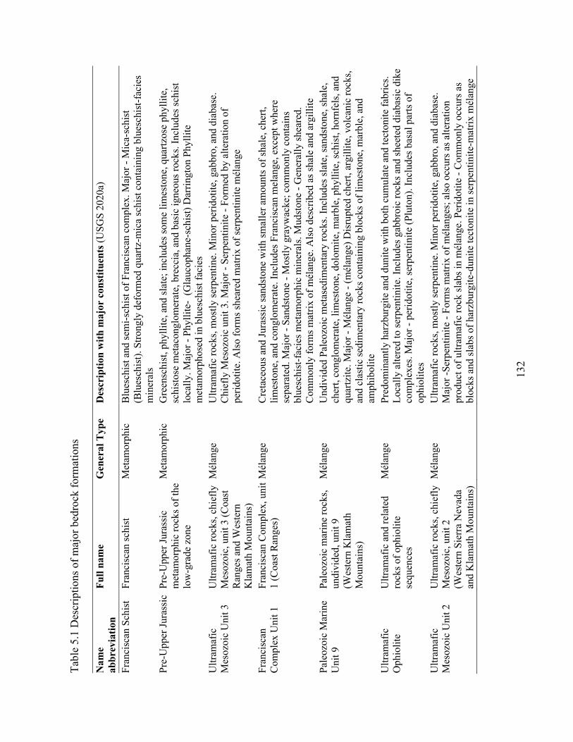
132
Tabl
e 5.
1 D
escr
iptio
ns o
f maj
or b
edro
ck fo
rmat
ions
Nam
e ab
brev
iatio
n Fu
ll na
me
Gen
eral
Typ
e D
escr
iptio
n w
ith m
ajor
con
stitu
ents
(USG
S 20
20a)
Fran
cisc
an S
chis
t Fr
anci
scan
sch
ist
Met
amor
phic
B
lues
chis
t and
sem
i-sc
hist
of
Fran
cisc
an c
ompl
ex. M
ajor
- M
ica-
schi
st
(Blu
esch
ist)
. Str
ongl
y de
form
ed q
uart
z-m
ica
schi
st c
onta
inin
g bl
uesc
hist
-fac
ies
min
eral
s Pr
e-U
pper
Jur
assi
c Pr
e-U
pper
Jur
assi
c m
etam
orph
ic r
ocks
of
the
low
-gra
de z
one
Met
amor
phic
G
reen
schi
st, p
hylli
te, a
nd s
late
; inc
lude
s so
me
limes
tone
, qua
rtzo
se p
hylli
te,
schi
stos
e m
etac
ongl
omer
ate,
bre
ccia
, and
bas
ic ig
neou
s ro
cks.
Inc
lude
s sc
hist
lo
cally
. Maj
or -
Phy
llite
- (
Gla
ucop
hane
-sch
ist)
Dar
ring
ton
Phyl
lite
met
amor
phos
ed in
blu
esch
ist f
acie
s U
ltram
afic
M
esoz
oic
Uni
t 3
Ultr
amaf
ic r
ocks
, chi
efly
M
esoz
oic,
uni
t 3 (
Coa
st
Ran
ges
and
Wes
tern
K
lam
ath
Mou
ntai
ns)
Mél
ange
U
ltram
afic
roc
ks, m
ostly
ser
pent
ine.
Min
or p
erid
otite
, gab
bro,
and
dia
base
. C
hief
ly M
esoz
oic
unit
3. M
ajor
- S
erpe
ntin
ite -
For
med
by
alte
ratio
n of
pe
rido
tite.
Als
o fo
rms
shea
red
mat
rix
of s
erpe
ntin
ite m
élan
ge
Fran
cisc
an
Com
plex
Uni
t 1
Fran
cisc
an C
ompl
ex, u
nit
1 (C
oast
Ran
ges)
M
élan
ge
Cre
tace
ous
and
Jura
ssic
san
dsto
ne w
ith s
mal
ler
amou
nts
of s
hale
, che
rt,
limes
tone
, and
con
glom
erat
e. I
nclu
des
Fran
cisc
an m
elan
ge, e
xcep
t whe
re
sepa
rate
d. M
ajor
- S
ands
tone
- M
ostly
gra
ywac
ke; c
omm
only
con
tain
s bl
uesc
hist
-fac
ies
met
amor
phic
min
eral
s. M
udst
one
- G
ener
ally
she
ared
. C
omm
only
for
ms
mat
rix
of m
élan
ge. A
lso
desc
ribe
d as
sha
le a
nd a
rgill
ite
Pale
ozoi
c M
arin
e U
nit 9
Pa
leoz
oic
mar
ine
rock
s,
undi
vide
d, u
nit 9
(W
este
rn K
lam
ath
Mou
ntai
ns)
Mél
ange
U
ndiv
ided
Pal
eozo
ic m
etas
edim
enta
ry r
ocks
. Inc
lude
s sl
ate,
san
dsto
ne, s
hale
, ch
ert,
cong
lom
erat
e, li
mes
tone
, dol
omite
, mar
ble,
phy
llite
, sch
ist,
horn
fels
, and
qu
artz
ite. M
ajor
- M
élan
ge -
(m
élan
ge)
Dis
rupt
ed c
hert
, arg
illite
, vol
cani
c ro
cks,
an
d cl
astic
sed
imen
tary
roc
ks c
onta
inin
g bl
ocks
of
limes
tone
, mar
ble,
and
am
phib
olite
U
ltram
afic
O
phio
lite
Ultr
amaf
ic a
nd r
elat
ed
rock
s of
oph
iolit
e se
quen
ces
Mél
ange
Pr
edom
inan
tly h
arzb
urgi
te a
nd d
unite
with
bot
h cu
mul
ate
and
tect
onite
fab
rics
. L
ocal
ly a
ltere
d to
ser
pent
inite
. Inc
lude
s ga
bbro
ic r
ocks
and
she
eted
dia
basi
c di
ke
com
plex
es. M
ajor
- p
erid
otite
, ser
pent
inite
(Pl
uton
). I
nclu
des
basa
l par
ts o
f op
hiol
ites
Ultr
amaf
ic
Mes
ozoi
c U
nit 2
U
ltram
afic
roc
ks, c
hief
ly
Mes
ozoi
c, u
nit 2
(W
este
rn S
ierr
a N
evad
a an
d K
lam
ath
Mou
ntai
ns)
Mél
ange
U
ltram
afic
roc
ks, m
ostly
ser
pent
ine.
Min
or p
erid
otite
, gab
bro,
and
dia
base
. M
ajor
-Se
rpen
tinite
- F
orm
s m
atri
x of
mél
ange
s; a
lso
occu
rs a
s al
tera
tion
prod
uct o
f ul
tram
afic
roc
k sl
abs
in m
élan
ge. P
erid
otite
- C
omm
only
occ
urs
as
bloc
ks a
nd s
labs
of
harz
burg
ite-d
unite
tect
onite
in s
erpe
ntin
ite-m
atri
x m
élan
ge
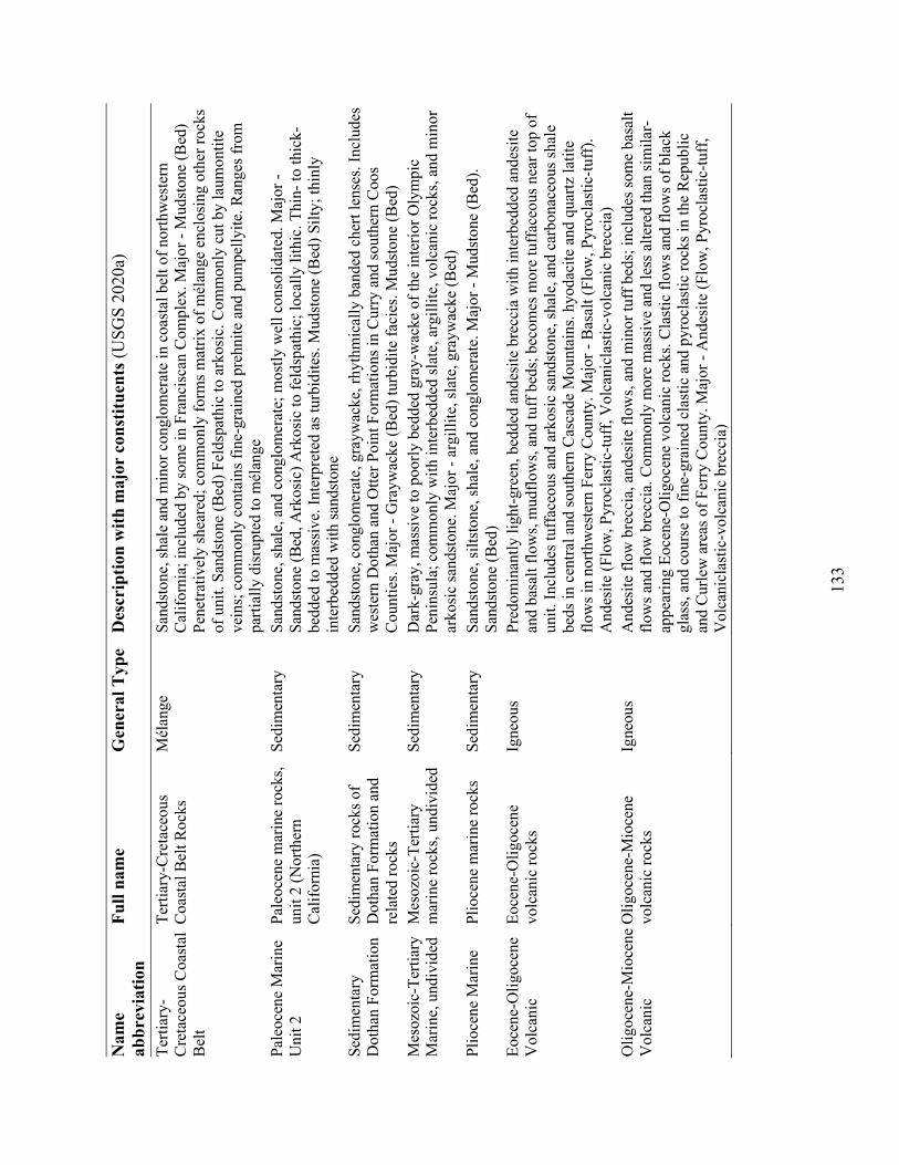
133
Nam
e ab
brev
iatio
n Fu
ll na
me
Gen
eral
Typ
e D
escr
iptio
n w
ith m
ajor
con
stitu
ents
(USG
S 20
20a)
Ter
tiary
-C
reta
ceou
s C
oast
al
Bel
t
Ter
tiary
-Cre
tace
ous
Coa
stal
Bel
t Roc
ks
Mél
ange
Sa
ndst
one,
sha
le a
nd m
inor
con
glom
erat
e in
coa
stal
bel
t of
nort
hwes
tern
C
alif
orni
a; in
clud
ed b
y so
me
in F
ranc
isca
n C
ompl
ex. M
ajor
- M
udst
one
(Bed
) Pe
netr
ativ
ely
shea
red;
com
mon
ly f
orm
s m
atri
x of
mél
ange
enc
losi
ng o
ther
roc
ks
of u
nit.
Sand
ston
e (B
ed)
Feld
spat
hic
to a
rkos
ic. C
omm
only
cut
by
laum
ontit
e ve
ins;
com
mon
ly c
onta
ins
fine
-gra
ined
pre
hnite
and
pum
pelly
ite. R
ange
s fr
om
part
ially
dis
rupt
ed to
mél
ange
Pa
leoc
ene
Mar
ine
Uni
t 2
Pale
ocen
e m
arin
e ro
cks,
un
it 2
(Nor
ther
n C
alif
orni
a)
Sedi
men
tary
Sa
ndst
one,
sha
le, a
nd c
ongl
omer
ate;
mos
tly w
ell c
onso
lidat
ed. M
ajor
-
Sand
ston
e (B
ed, A
rkos
ic)
Ark
osic
to f
elds
path
ic; l
ocal
ly li
thic
. Thi
n- to
thic
k-be
dded
to m
assi
ve. I
nter
pret
ed a
s tu
rbid
ites.
Mud
ston
e (B
ed)
Silty
; thi
nly
inte
rbed
ded
with
san
dsto
ne
Sedi
men
tary
D
otha
n Fo
rmat
ion
Sedi
men
tary
roc
ks o
f D
otha
n Fo
rmat
ion
and
rela
ted
rock
s
Sedi
men
tary
Sa
ndst
one,
con
glom
erat
e, g
rayw
acke
, rhy
thm
ical
ly b
ande
d ch
ert l
ense
s. I
nclu
des
wes
tern
Dot
han
and
Otte
r Po
int F
orm
atio
ns in
Cur
ry a
nd s
outh
ern
Coo
s C
ount
ies.
Maj
or -
Gra
ywac
ke (
Bed
) tu
rbid
ite f
acie
s. M
udst
one
(Bed
) M
esoz
oic-
Ter
tiary
M
arin
e, u
ndiv
ided
M
esoz
oic-
Ter
tiary
m
arin
e ro
cks,
und
ivid
ed
Sedi
men
tary
D
ark-
gray
, mas
sive
to p
oorl
y be
dded
gra
y-w
acke
of
the
inte
rior
Oly
mpi
c Pe
nins
ula;
com
mon
ly w
ith in
terb
edde
d sl
ate,
arg
illite
, vol
cani
c ro
cks,
and
min
or
arko
sic
sand
ston
e. M
ajor
- a
rgill
ite, s
late
, gra
ywac
ke (
Bed
) Pl
ioce
ne M
arin
e Pl
ioce
ne m
arin
e ro
cks
Sedi
men
tary
Sa
ndst
one,
silt
ston
e, s
hale
, and
con
glom
erat
e. M
ajor
- M
udst
one
(Bed
).
Sand
ston
e (B
ed)
Eoc
ene-
Olig
ocen
e V
olca
nic
Eoc
ene-
Olig
ocen
e vo
lcan
ic r
ocks
Ig
neou
s Pr
edom
inan
tly li
ght-
gree
n, b
edde
d an
desi
te b
recc
ia w
ith in
terb
edde
d an
desi
te
and
basa
lt fl
ows,
mud
flow
s, a
nd tu
ff b
eds;
bec
omes
mor
e tu
ffac
eous
nea
r to
p of
un
it. I
nclu
des
tuff
aceo
us a
nd a
rkos
ic s
ands
tone
, sha
le, a
nd c
arbo
nace
ous
shal
e be
ds in
cen
tral
and
sou
ther
n C
asca
de M
ount
ains
. hyo
daci
te a
nd q
uart
z la
tite
flow
s in
nor
thw
este
rn F
erry
Cou
nty.
Maj
or -
Bas
alt (
Flow
, Pyr
ocla
stic
-tuf
f).
And
esite
(Fl
ow, P
yroc
last
ic-t
uff,
Vol
cani
clas
tic-v
olca
nic
brec
cia)
O
ligoc
ene-
Mio
cene
V
olca
nic
Olig
ocen
e-M
ioce
ne
volc
anic
roc
ks
Igne
ous
And
esite
flo
w b
recc
ia, a
ndes
ite f
low
s, a
nd m
inor
tuff
bed
s; in
clud
es s
ome
basa
lt fl
ows
and
flow
bre
ccia
. Com
mon
ly m
ore
mas
sive
and
less
alte
red
than
sim
ilar-
appe
arin
g E
ocen
e-O
ligoc
ene
volc
anic
roc
ks. C
last
ic f
low
s an
d fl
ows
of b
lack
gl
ass,
and
cou
rse
to f
ine-
grai
ned
clas
tic a
nd p
yroc
last
ic r
ocks
in th
e R
epub
lic
and
Cur
lew
are
as o
f Fe
rry
Cou
nty.
Maj
or -
And
esite
(Fl
ow, P
yroc
last
ic-t
uff,
V
olca
nicl
astic
-vol
cani
c br
ecci
a)
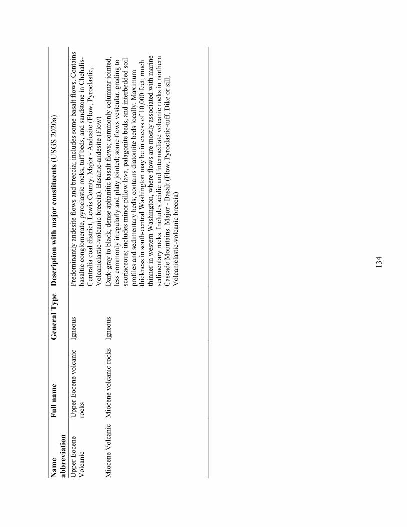
134
Nam
e ab
brev
iatio
n Fu
ll na
me
Gen
eral
Typ
e D
escr
iptio
n w
ith m
ajor
con
stitu
ents
(USG
S 20
20a)
Upp
er E
ocen
e V
olca
nic
Upp
er E
ocen
e vo
lcan
ic
rock
s Ig
neou
s Pr
edom
inan
tly a
ndes
ite f
low
s an
d br
ecci
a; in
clud
es s
ome
basa
lt fl
ows.
Con
tain
s ba
salti
c co
nglo
mer
ate,
pyr
ocla
stic
roc
ks, t
uff
beds
, and
san
dsto
ne in
Che
halis
-C
entr
alia
coa
l dis
tric
t, L
ewis
Cou
nty.
Maj
or -
And
esite
(Fl
ow, P
yroc
last
ic,
Vol
cani
clas
tic-v
olca
nic
brec
cia)
. Bas
altic
-and
esite
(Fl
ow)
Mio
cene
Vol
cani
c M
ioce
ne v
olca
nic
rock
s Ig
neou
s D
ark-
gray
to b
lack
, den
se a
phan
itic
basa
lt fl
ows;
com
mon
ly c
olum
nar
join
ted,
le
ss c
omm
only
irre
gula
rly
and
plat
y jo
inte
d; s
ome
flow
s ve
sicu
lar,
gra
ding
to
scor
iace
ous;
incl
udes
min
or p
illow
lava
, pal
agon
ite b
eds,
and
inte
rbed
ded
soil
prof
iles
and
sedi
men
tary
bed
s; c
onta
ins
diat
omite
bed
s lo
cally
. Max
imum
th
ickn
ess
in s
outh
-cen
tral
Was
hing
ton
may
be
in e
xces
s of
10,
000
feet
; muc
h th
inne
r in
wes
tern
Was
hing
ton,
whe
re f
low
s ar
e m
ostly
ass
ocia
ted
with
mar
ine
sedi
men
tary
roc
ks. I
nclu
des
acid
ic a
nd in
term
edia
te v
olca
nic
rock
s in
nor
ther
n C
asca
de M
ount
ains
. Maj
or -
Bas
alt (
Flow
, Pyr
ocla
stic
-tuf
f, D
ike
or s
ill,
Vol
cani
clas
tic-v
olca
nic
brec
cia)
135
5.2.4 Landslide Area-volume Scaling and Average Slope Angle
A power-law relationship between landslide volume, !, and landslide surface area, ", was
used to estimate landslide volumes in varied bedrock (Larson et al., 2010):
! ∝ "!(5.3)
where * is a scaling exponent. We used * = 1.6 for the identified large, deep-seated landslides
(Larson et al., 2010). Surface areas of landslides were computed from the landslide boundary (Xu
et al., 2020b) outlined from SAR interferograms.
The slope angle of each DEM cell element was derived from the 10-meter-resolution DEMs.
Each identified landslide spatially covers multiple DEM cell elements, and we define the average
slope angle of a landslide as the arithmetic mean of all cell elements within the landslide boundary.
5.2.5 Land Uplift Rate
Land uplift rates in the U.S. west coast states were obtained by evaluating published literature
on geologically and historically recent vertical land movement. This literature (Table 5.2) includes
studies emphasizing land surface surveying (Amos et al., 2014; Hammond et al., 2016; Levy, 2019;
Yousefi et al., 2020) during recent times, or geologic studies generally extending from recent times
into the Quaternary and Neogene Periods (Bennett et al., 2016a; Amos et al., 2014; Levy, 2019;
Yousefi et al., 2020; Anderson, 2008; Barth and May, 1992; Hellwig, 2010; House, 1999; Jones,
1987; Kesley and Bockheim, 1994; Kobor and Roering, 2004; Lock et al., 2006; Machette et al.,
1984; Muhs et al., 1992; Pazzaglia and Brandon, 2001; Penserini et al., 2017; Reiners et al., 2002;
Schweickert, 2009; Spotila et al., 1998; Unruh, 1991). Longer-term studies emphasized fluvial and
coastal geomorphology, often with cosmogenic nuclide and/or radionuclide dating,
thermochronology, and modeling. We interpolated these pointwise uplift data into a gridded raster
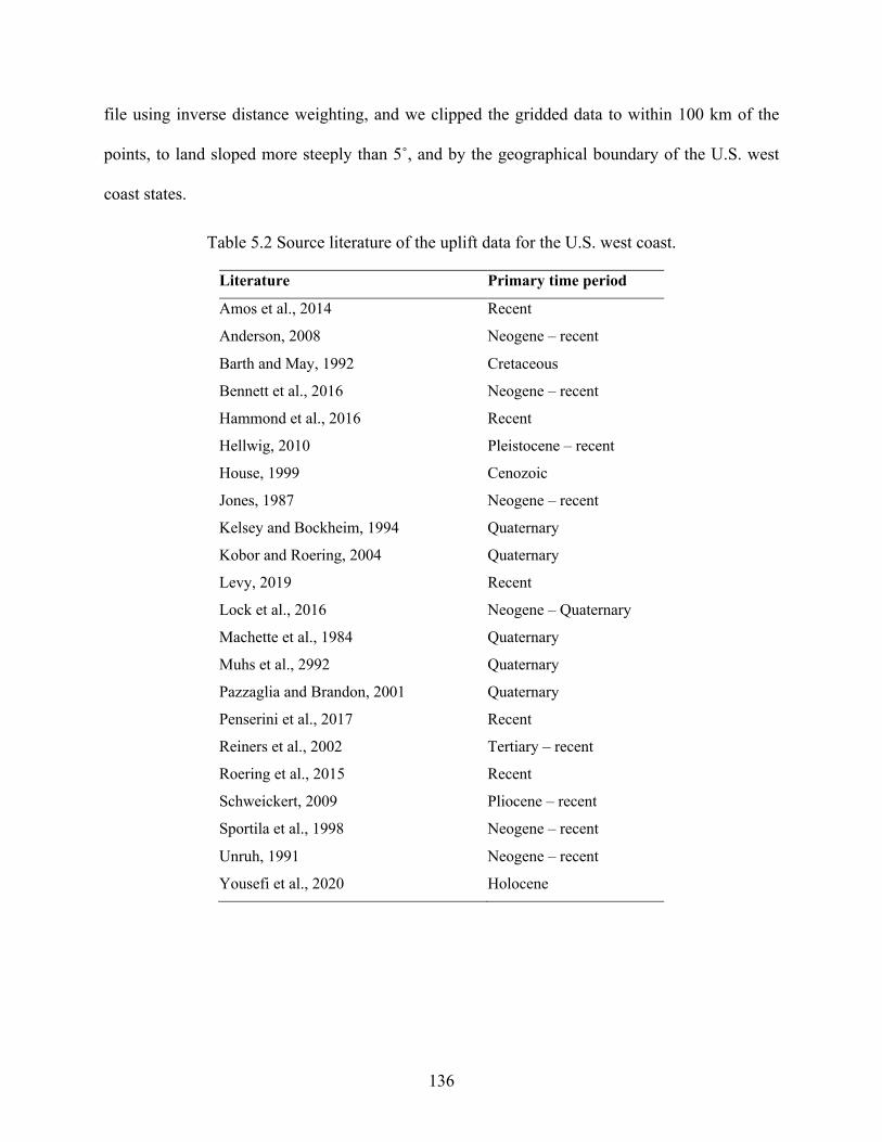
136
file using inverse distance weighting, and we clipped the gridded data to within 100 km of the
points, to land sloped more steeply than 5˚, and by the geographical boundary of the U.S. west
coast states.
Table 5.2 Source literature of the uplift data for the U.S. west coast.
Literature Primary time period
Amos et al., 2014 Recent
Anderson, 2008 Neogene – recent
Barth and May, 1992 Cretaceous
Bennett et al., 2016 Neogene – recent
Hammond et al., 2016 Recent
Hellwig, 2010 Pleistocene – recent
House, 1999 Cenozoic
Jones, 1987 Neogene – recent
Kelsey and Bockheim, 1994 Quaternary
Kobor and Roering, 2004 Quaternary
Levy, 2019 Recent
Lock et al., 2016 Neogene – Quaternary
Machette et al., 1984 Quaternary
Muhs et al., 2992 Quaternary
Pazzaglia and Brandon, 2001 Quaternary
Penserini et al., 2017 Recent
Reiners et al., 2002 Tertiary – recent
Roering et al., 2015 Recent
Schweickert, 2009 Pliocene – recent
Sportila et al., 1998 Neogene – recent
Unruh, 1991 Neogene – recent
Yousefi et al., 2020 Holocene
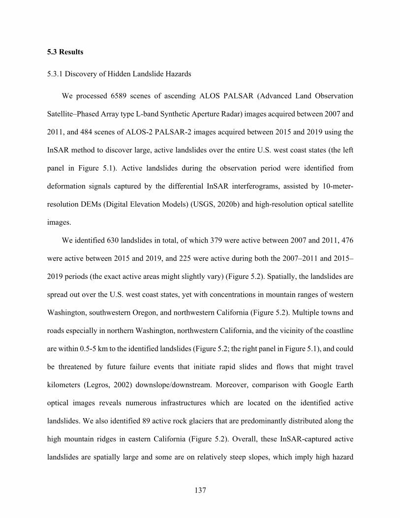
137
5.3 Results
5.3.1 Discovery of Hidden Landslide Hazards
We processed 6589 scenes of ascending ALOS PALSAR (Advanced Land Observation
Satellite–Phased Array type L-band Synthetic Aperture Radar) images acquired between 2007 and
2011, and 484 scenes of ALOS-2 PALSAR-2 images acquired between 2015 and 2019 using the
InSAR method to discover large, active landslides over the entire U.S. west coast states (the left
panel in Figure 5.1). Active landslides during the observation period were identified from
deformation signals captured by the differential InSAR interferograms, assisted by 10-meter-
resolution DEMs (Digital Elevation Models) (USGS, 2020b) and high-resolution optical satellite
images.
We identified 630 landslides in total, of which 379 were active between 2007 and 2011, 476
were active between 2015 and 2019, and 225 were active during both the 2007–2011 and 2015–
2019 periods (the exact active areas might slightly vary) (Figure 5.2). Spatially, the landslides are
spread out over the U.S. west coast states, yet with concentrations in mountain ranges of western
Washington, southwestern Oregon, and northwestern California (Figure 5.2). Multiple towns and
roads especially in northern Washington, northwestern California, and the vicinity of the coastline
are within 0.5-5 km to the identified landslides (Figure 5.2; the right panel in Figure 5.1), and could
be threatened by future failure events that initiate rapid slides and flows that might travel
kilometers (Legros, 2002) downslope/downstream. Moreover, comparison with Google Earth
optical images reveals numerous infrastructures which are located on the identified active
landslides. We also identified 89 active rock glaciers that are predominantly distributed along the
high mountain ridges in eastern California (Figure 5.2). Overall, these InSAR-captured active
landslides are spatially large and some are on relatively steep slopes, which imply high hazard
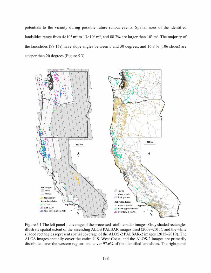
138
potentials to the vicinity during possible future runout events. Spatial sizes of the identified
landslides range from 4×10⁴ m2 to 13×106 m2, and 88.7% are larger than 105 m2. The majority of
the landslides (97.1%) have slope angles between 5 and 30 degrees, and 16.8 % (106 slides) are
steeper than 20 degrees (Figure 5.3).
Figure 5.1 The left panel – coverage of the processed satellite radar images. Gray shaded rectangles illustrate spatial extent of the ascending ALOS PALSAR images used (2007–2011), and the white shaded rectangles represent spatial coverage of the ALOS-2 PALSAR-2 images (2015–2019). The ALOS images spatially cover the entire U.S. West Coast, and the ALOS-2 images are primarily distributed over the western regions and cover 97.6% of the identified landslides. The right panel
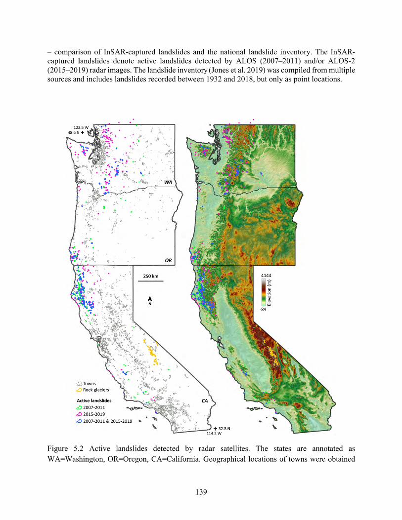
139
– comparison of InSAR-captured landslides and the national landslide inventory. The InSAR-captured landslides denote active landslides detected by ALOS (2007–2011) and/or ALOS-2 (2015–2019) radar images. The landslide inventory (Jones et al. 2019) was compiled from multiple sources and includes landslides recorded between 1932 and 2018, but only as point locations.
Figure 5.2 Active landslides detected by radar satellites. The states are annotated as WA=Washington, OR=Oregon, CA=California. Geographical locations of towns were obtained
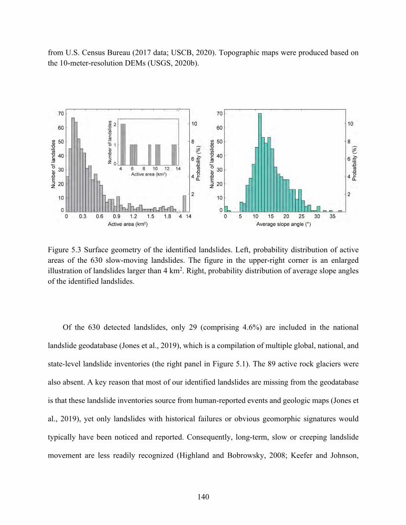
140
from U.S. Census Bureau (2017 data; USCB, 2020). Topographic maps were produced based on the 10-meter-resolution DEMs (USGS, 2020b).
Figure 5.3 Surface geometry of the identified landslides. Left, probability distribution of active areas of the 630 slow-moving landslides. The figure in the upper-right corner is an enlarged illustration of landslides larger than 4 km2. Right, probability distribution of average slope angles of the identified landslides.
Of the 630 detected landslides, only 29 (comprising 4.6%) are included in the national
landslide geodatabase (Jones et al., 2019), which is a compilation of multiple global, national, and
state-level landslide inventories (the right panel in Figure 5.1). The 89 active rock glaciers were
also absent. A key reason that most of our identified landslides are missing from the geodatabase
is that these landslide inventories source from human-reported events and geologic maps (Jones et
al., 2019), yet only landslides with historical failures or obvious geomorphic signatures would
typically have been noticed and reported. Consequently, long-term, slow or creeping landslide
movement are less readily recognized (Highland and Bobrowsky, 2008; Keefer and Johnson,
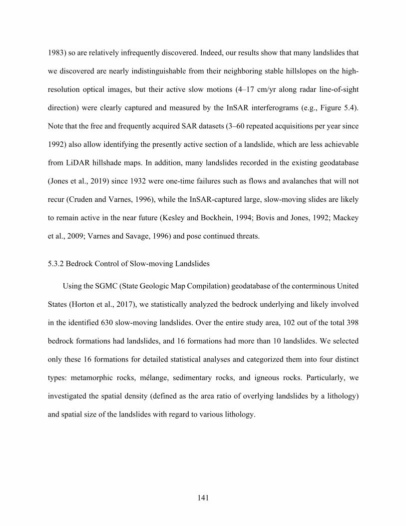
141
1983) so are relatively infrequently discovered. Indeed, our results show that many landslides that
we discovered are nearly indistinguishable from their neighboring stable hillslopes on the high-
resolution optical images, but their active slow motions (4–17 cm/yr along radar line-of-sight
direction) were clearly captured and measured by the InSAR interferograms (e.g., Figure 5.4).
Note that the free and frequently acquired SAR datasets (3–60 repeated acquisitions per year since
1992) also allow identifying the presently active section of a landslide, which are less achievable
from LiDAR hillshade maps. In addition, many landslides recorded in the existing geodatabase
(Jones et al., 2019) since 1932 were one-time failures such as flows and avalanches that will not
recur (Cruden and Varnes, 1996), while the InSAR-captured large, slow-moving slides are likely
to remain active in the near future (Kesley and Bockhein, 1994; Bovis and Jones, 1992; Mackey
et al., 2009; Varnes and Savage, 1996) and pose continued threats.
5.3.2 Bedrock Control of Slow-moving Landslides
Using the SGMC (State Geologic Map Compilation) geodatabase of the conterminous United
States (Horton et al., 2017), we statistically analyzed the bedrock underlying and likely involved
in the identified 630 slow-moving landslides. Over the entire study area, 102 out of the total 398
bedrock formations had landslides, and 16 formations had more than 10 landslides. We selected
only these 16 formations for detailed statistical analyses and categorized them into four distinct
types: metamorphic rocks, mélange, sedimentary rocks, and igneous rocks. Particularly, we
investigated the spatial density (defined as the area ratio of overlying landslides by a lithology)
and spatial size of the landslides with regard to various lithology.
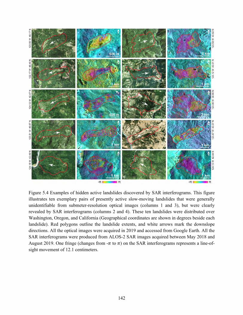
142
Figure 5.4 Examples of hidden active landslides discovered by SAR interferograms. This figure illustrates ten exemplary pairs of presently active slow-moving landslides that were generally unidentifiable from submeter-resolution optical images (columns 1 and 3), but were clearly revealed by SAR interferograms (columns 2 and 4). These ten landslides were distributed over Washington, Oregon, and California (Geographical coordinates are shown in degrees beside each landslide). Red polygons outline the landslide extents, and white arrows mark the downslope directions. All the optical images were acquired in 2019 and accessed from Google Earth. All the SAR interferograms were produced from ALOS-2 SAR images acquired between May 2018 and August 2019. One fringe (changes from -. to .) on the SAR interferograms represents a line-of-sight movement of 12.1 centimeters.
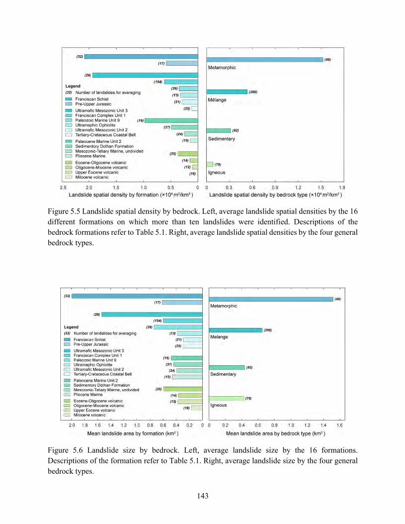
143
Figure 5.5 Landslide spatial density by bedrock. Left, average landslide spatial densities by the 16 different formations on which more than ten landslides were identified. Descriptions of the bedrock formations refer to Table 5.1. Right, average landslide spatial densities by the four general bedrock types.
Figure 5.6 Landslide size by bedrock. Left, average landslide size by the 16 formations. Descriptions of the formation refer to Table 5.1. Right, average landslide size by the four general bedrock types.
144
Our results demonstrate that both spatial density and size of the identified slow-moving
landslides were strongly controlled by their lithology. By bedrock type, the greatest spatial density
was found in metamorphic rocks (15,300 m2/km2), followed by mélange (5400 m2/km2),
sedimentary rocks (3200 m2/km2), and igneous rocks (1300 m2/km2) (Figure 4). Similar trends
were also found in their spatial sizes. The largest mean size was in metamorphic rocks (1.52 km2),
then mélange (0.6 km2), and similar in sedimentary (0.44 km2) and igneous rocks (0.43 km2)
(Figure 5). Overall, landslides were largest and most frequent in metamorphic rocks followed by
mélange, and the spatial density and mean size were 3 to 12 times greater in metamorphic rocks
than in sedimentary and igneous rocks. The results also indicate that these presently active
landslides are presenting hazards from and modifying landscapes of mélange bedrock to the
greatest extent. Assuming similar area-volume scaling (Larson et al., 2010) for landslides in each
of the bedrock types, the results indicate that slow-moving landslides in mélange have mobilized
1.4, 8.6, and 10.6 times the sediment of landslides in metamorphic, igneous, and sedimentary
rocks, respectively.
The greater size and density of slow-moving landslides in metamorphic rocks and mélange
compared to igneous and sedimentary rocks may partly result from generally lower rock mass
strength due to pervasive discontinuities in foliated and tectonically sheared metamorphic rocks
and mélange (Cruden and Varnes, 1996), as well as the relatively high abundance of clay minerals
in these altered rocks (Lambe and Whitman, 1969; Schmidt and Montgomery, 1995). In addition,
igneous rocks in which landslides were identified were mostly andesite and basalt flows (Table
5.1). Flows and sedimentary rock are likely to have spatially extensive discontinuities between
beds and flow units, and relatively high anisotropy of material properties because of their layered
nature (Jaeger et al., 2009). Such discontinuities and anisotropy are relatively lacking from most
145
metamorphic and mélange rock formations (Jaeger et al., 2009). Shallower and therefore smaller
landslides are more likely in materials with such anisotropy (Cruden and Varnes, 1996), whereas
deeper and therefore larger landslides are more likely in more isotropic materials (Cruden and
Varnes, 2996), such as mélange and metamorphic rocks.
5.3.3 Landsliding Contributed by Land Uplift
We investigated how vertical land motion may relate to the identified slow-moving landslides
by incorporating vertical motion data for the study area from radioisotope dating, modeling and
recent observations (Table 5.2). We expect that land uplift results in and sustains continuous
landsliding because uplift creates topographic relief resulting in stream downcutting and hillslope
instability (Burbank et al., 1996; Roering et al., 2005; Cruden and Varnes, 1996; Lambe and
Whitman, 1969; Larson and Montgometry, 2012; Bennett et al., 2016a). Slow-moving landslides
identifiable from InSAR may be very long lived (102–104 years) (Bovis and Jones, 1992; Varnes
and Savage, 1996; Mackey et al., 2009; Keefer and Johnson, 1983) and usually continue moving
during dry periods or reactivate thereafter (Bovis and Jones, 1992; Bennett et al., 2016b; Skempton
et al., 1989; Coe, 2012), thus their occurrence and persistent long-term creeping motions most
likely have been greatly contributed to and/or sustained by geologically recent (103–105 years)
uplift. However, although less sensitive to recent rainfall than small landslides, large landslides
are strongly modulated by precipitation on a short timescale such as seasonal movement (Coe,
2012; Bennett et al., 2016b). Here we only focus on the potential contributions from long-term
land uplift, and the short-timescale hydrological contributions are detailed in the Discussion
section.
146
Land surface uplift measurements from a total of 79 sites over the study area were converted
to gridded data using the inverse distance weighted interpolation in order to compare uplift rates
at landslide locations to those at stable regions. We excluded the regions with slope angle less than
5˚ in the analysis as our observations show that landslides barely occur in such flat terrain (Figure
2). Our analyses reveal that the 630 landslides and the 89 rock glaciers were geographically related
to geologic uplift. Overall, the rapidly uplifting northwestern Washington, southwestern Oregon,
northwestern California, coastal regions of southern California, and high mountains of middle-east
California all saw a great number of active landslides or rock glaciers, while the subsiding middle-
west Oregon, middle-west California, and the southern end of Sierra Nevada Mountains (middle-
east California) were barely involved with any identified landslides (Figure 6). Quantitatively, the
uplift rates at the active landslides and rock glaciers average 0.83 mm/yr, three times higher than
the mean rate of 0.27 mm/yr for the whole region (Table 5.3). The results are also insensitive to
the excluded flat regions: thresholding slope angles at 0˚, 10˚, and 16˚ would yield mean uplift
rates of 0.79 mm/yr over 0.12 mm/yr (landslides versus the whole region), 0.83 mm/yr over 0.30
mm/yr, and 0.82 mm/yr over 0.32 mm/yr, respectively (Table 5.3). All of the results provide
evidence that the identified slow-moving landslides were preferentially located in areas with
accelerated geologically recent uplift. We expect that rapid and/or small landslides similarly
collocate with accelerated uplift, but InSAR does not well resolve rapid and/or small landslides.
147
Table 5.3 Uplift rates by excluding flat regions. Regions with slope less steep than the slope angle threshold were excluded from the corresponding results.
Slope angle
threshold (˚)
Regions Minimum rate
(mm/yr)
Maximum
rate (mm/yr)
Mean rate
(mm/yr)
Standard deviation
(mm/yr)
0 Landslides -0.62 2.86 0.79 0.59
All regions -3 5 0.12 0.65
5 Landslides -0.62 2.86 0.83 0.58
All regions -2.99 4.72 0.27 0.57
10 Landslides -0.62 2.86 0.83 0.56
All regions -2.96 4.72 0.3 0.56
16 Landslides -0.62 2.86 0.82 0.53
All regions -2.95 4.72 0.32 0.55
5.4 Discussion and Conclusions
5.4.1 Landslide Identification Using Radar Interferometry
We revealed 630 active, large, potentially dangerous landslides hidden in the U.S. west coast
states, 601 of which are missing from existing landslide inventories that source from geologic
maps and citizen reports (Jones et al. 2019). These actively moving landslides are the most
significant agents for regional landscape modification and are potential hazards to residents and
infrastructure in the vicinity. We found that the high-accuracy InSAR tool could be effective in
uncovering their locations, boundaries, and motions.
InSAR is relatively less sensitive to landslide motions that are orientated perpendicular to the
radar look direction. However, mountain ranges near the U.S. west coast are dominantly north-
south orientated and has formed landslides which are mostly visible from the approximately
west/east looking radar sensor. Moreover, we utilized SAR interferograms spanning as long as two
148
years for landslide identification, and such long timespan allow landslides to accumulate a large
displacement that is clearly identifiable on SAR interferograms.
Figure 5.7 Vertical land motions near the U.S. west coast. Left, vertical uplift (green) and subsidence (red) rates of the 79 sites shown in solid circles. Right, an interpolated map produced from the point-wise measurements. Only hillslopes steeper than 5˚ and within 100 km distant from the measurement sites are shown in the figure.
149
5.4.2 Geologic Impacts on Landslide Character and Kinematics
We found that bedrock lithology exerts significant control on both the spatial density and size
of the slow-moving landslides. Metamorphic rocks and mélange that have relatively homogeneous
composition, discontinuity distribution, and high clay content, while also having relatively low
shear strength, are most likely to bear widespread, deep, and large slow-moving landslides. In
contrast, sedimentary and igneous flow rocks that have strength and hydrologic anisotropy and
relatively high shear strength tend to produce relatively sparse, shallow, and small slow-moving
landslides.
Our observations also provide evidence that geologic uplift is a crucial contributor to the
occurrence and long-term creeping behavior of the slow-moving landslides. Both the identified
active rock glaciers and slow-moving landslides are predominantly distributed over hillslopes with
geologically recent (103–105 years), accelerated uplift, but barely observed in geologically
subsiding terrains, implying a fundamental control from vertical land motion. The contributions
from land uplift are a gradually cumulative effect, and such signal could be overwhelmed and
clouded by other short-timescale factors (particularly precipitation). Long-term land uplift creates
mountains resulting in hillslope instability, and landslide is the process to restabilize a hillslope.
Hence, it is essentially land uplift that results in mountain landslides, though precipitation is often
seen being the “trigger” for landslide initiation and seasonal acceleration.
5.4.3 Hydrological Impacts on Landslide Motion
On an annual scale, precipitation is widely recognized as the driver for seasonal acceleration
and deceleration of slow-moving landslides (Xu at al., 2020; Squarzoni et al., 2003; Ye et al., 2004;
Xu et al., 2019; Bennett et al., 2016b; Handwerger et al., 2019). However, precipitation may not
be the only reason to initiate a landslide or keep a slow-moving landslide constantly active for
150
hundreds of years (Kesley and Bockheim, 1994; Bonzanigo et al., 2007; Roering et al., 2015). We
compared 30-year average precipitation (1981-2010) relative to observed landslide locations
(Figure 5.8) and found that precipitation amount at those locations is highly variable. Overall, 75%
of the identified large and slowly moving landslides are located in the mountain ranges that receive
relatively rich rainfall (≥ 2000 mm). However, numerous exceptions were found in central
Washington and south-western California, where relatively dry lands (approximately 400 mm
annual rainfall) produced about 90 landslides. Moreover, the rainfall-abundant (over 2500 mm)
southern Cascade ranges and northern coastal ranges of Oregon only included 12 landslides, far
fewer than the north-western California where 1800 mm of annual rainfall produced 484 landslides
(Figure 5.8). In addition, we compared the identified landslides with the average excess
precipitation between 2016 and 2019 (the right panel in Figure 5.8). Here excess precipitation is
defined as the difference between annual precipitation and the 30-year average. The results show
that numerous landslides in particularly southern Washington and southwestern Oregon were
captured active during even the historically dry years between 2016 and 2019. Therefore,
precipitation alone cannot well explain the spatial distribution of the identified slow-moving
landslides.
The precipitation distribution near the U.S. west coast is not independent from land uplift. In
fact, annual precipitation positively correlates with elevation (Daly et al., 2017) because the warm
air coming from Pacific Ocean condenses to form cloud droplets while climbing up the high
mountains and produces precipitation. As evidenced in Figure 5.8, heavy precipitation dominantly
falls on the high mountains of the coastal ranges, Cascade Ranges, and the Sierra-Nevada Ranges.
Consequently, land uplift not only leads to landsliding by creating high relief, but also contributes
to hillslope instability by increasing precipitation over a geological timescale. In addition, the
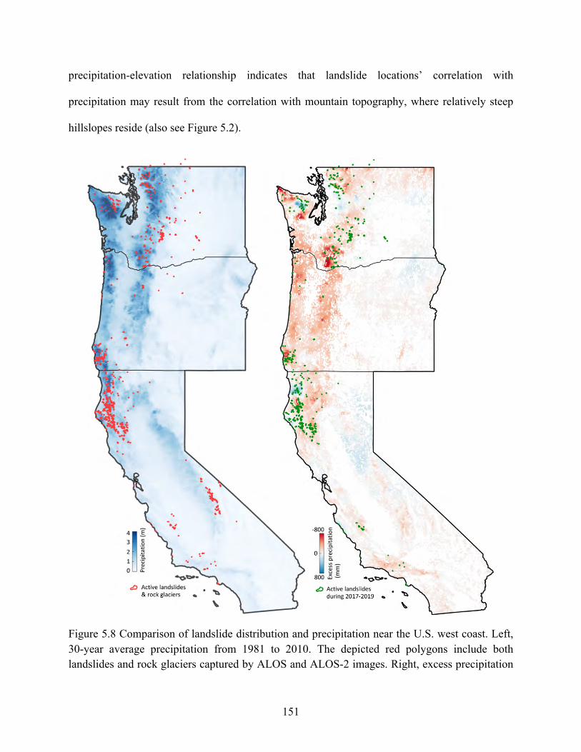
151
precipitation-elevation relationship indicates that landslide locations’ correlation with
precipitation may result from the correlation with mountain topography, where relatively steep
hillslopes reside (also see Figure 5.2).
Figure 5.8 Comparison of landslide distribution and precipitation near the U.S. west coast. Left, 30-year average precipitation from 1981 to 2010. The depicted red polygons include both landslides and rock glaciers captured by ALOS and ALOS-2 images. Right, excess precipitation
152
(average annual precipitation subtracts the 30-year average) from 2017 to 2019. The green polygons only depict landslides which were active between 2017 and 2019.
5.4.4 Implication on Landslide and Geomorphic Studies
Failure events initiated from slow-moving landslides have caused considerable
socioeconomic loss globally in recent decades (Schuster and Highland, 2001; Froude and Petley,
2018; Kilburn and Petley, 2003; Intrieri et al., 2018; Xu et al., 2020b), and many damages
(especially casualties) could have been avoided if the precursory slow motions were revealed prior
to the catastrophes. The routinely acquired (optimal every 6 days; ESA, 2020) and globally
covered satellite radar images could prove valuable in uncovering such hidden landslides for
mitigating future hazards, especially in response to the predicted increasingly frequent landslide
activities owing to global climate change and expanding anthropogenic activities (Gariano and
Guzzetti, 2016; Froude and Petley, 2018). In addition, the fundamental controls of slow-moving
landslides by bedrock and vertical land motion could offer novel insights for landslide
susceptibility forecasting and landform evolution studies. Globally, the geologically recent uplifts
in the Himalayan mountains (Asia) (Ader et al., 2012), Alps mountains (Europe) (Sternai, 2019),
Pacific West Coast (North America) (Muhs et al., 1992), and Andes mountains (South America)
(Armijo et al., 2015) are expected to fuel continued landslide hazards and intensify
geomorphological change. However, regional tectonic subsidence within these mountain ranges
may conversely attenuate local landslide activities.
153
ACKNOWLEDGEMENTS
We acknowledge the Japan Aerospace Exploration Agency for acquiring the ALOS PALSAR
and ALOS-2 PALSAR-2 images, and we thank the 3D Elevation Program Group of the United
States Geological Survey for producing and making available the 10-meter-resolution DEMs. We
also thank the authors listed in Table 5.2 for producing the uplift data. This study was funded by
NASA Interdisciplinary Research (IDS) in Earth Science Program (80NSSC17K0022), NASA
Earth Surface and Interior Focus Area (80NSSC19K1491), and the USGS Landslide Hazards
Program. Any use of trade, firm, or product names is for descriptive purposes only and does not
imply endorsement by the U.S. Government.
The ALOS PALSAR data are freely accessible from the Alaska Satellite Facility
(https://asf.alaska.edu/), and the ALOS-2 PALSAR-2 data are obtainable from Japan Aerospace
Exploration Agency (https://auig2.jaxa.jp/). The 10-meter-resolution DEMs covering the U.S.
west coast states are freely available from U.S. Geological Survey
(http://usgs.gov/NationalMap/data/), and the high-resolution true color images are available from
Google Earth. Shapefiles of towns and state boundaries of the U.S. west coast states are
downloadable from U.S. Census Bureau (https://www.census.gov/cgi-bin/geo/shapefiles/). The
State Geologic Map Compilation (SGMC) geodatabase of the conterminous United States is
available from U.S. Geological Survey (USGS, 2020a). The PRISM precipitation data are freely
available from the PRISM Cimate Group (https://prism.oregonstate.edu/). Shapefiles depicting

154
landslides identified during this study are available from the U.S. Geological Survey ScienceBase
repository (Xu et al. 2020a).
155
REFERENCES
Ader, T., Avouac, J. P., Liu‐Zeng, J., Lyon‐Caen, H., Bollinger, L., Galetzka, J., ... and Flouzat, M. (2012). Convergence rate across the Nepal Himalaya and interseismic coupling on the Main Himalayan Thrust: Implications for seismic hazard. Journal of Geophysical Research: Solid Earth, 117(B4).
Amos, C. B., Audet, P., Hammond, W. C., Bürgmann, R., Johanson, I. A., and Blewitt, G. (2014). Uplift and seismicity driven by groundwater depletion in central California. Nature, 509(7501), 483-486.
Anderson, T. K. (2008). Inferring bedrock uplift in the Klamath Mountains Province from river profile analysis and digital topography (Doctoral dissertation, Texas Tech University).
Armijo, R., Lacassin, R., Coudurier-Curveur, A., and Carrizo, D. (2015). Coupled tectonic evolution of Andean orogeny and global climate. Earth-Science Reviews, 143, 1-35.
Barth, A. P., and May, D. J. (1992). Mineralogy and pressure–temperature–time path of Cretaceous granulite gneisses, south‐eastern San Gabriel Mountains, southern California. Journal of Metamorphic Geology, 10(4), 529-544.
Bennett, G. L., Miller, S. R., Roering, J. J., and Schmidt, D. A. (2016). Landslides, threshold slopes, and the survival of relict terrain in the wake of the Mendocino Triple Junction. Geology, 44(5), 363-366.
Bonzanigo, L., Eberhardt, E., and Loew, S. (2007). Long-term investigation of a deep-seated creeping landslide in crystalline rock. Part I. Geological and hydromechanical factors controlling the Campo Vallemaggia landslide. Canadian Geotechnical Journal, 44(10), 1157-1180.
Bovis, M. J., and Jones, P. (1992). Holocene history of earthflow mass movements in south-central British Columbia: the influence of hydroclimatic changes. Canadian Journal of Earth Sciences, 29(8), 1746-1755.
Burbank, D. W., Leland, J., Fielding, E., Anderson, R. S., Brozovic, N., Reid, M. R., and Duncan, C. (1996). Bedrock incision, rock uplift and threshold hillslopes in the northwestern Himalayas. Nature, 379(6565), 505-510.
Clarke, B. A., and Burbank, D. W. (2010). Bedrock fracturing, threshold hillslopes, and limits to the magnitude of bedrock landslides. Earth and Planetary Science Letters, 297(3-4), 577-586.
156
Coe, J. A. (2012). Regional moisture balance control of landslide motion: Implications for landslide forecasting in a changing climate. Geology, 40(4), 323-326.
Costantini, M. (1998). A novel phase unwrapping method based on network programming. IEEE Transactions on geoscience and remote sensing, 36(3), 813-821.
Cruden, D. M., Varnes, D. J. (1996) in Landslides, Investigation and Mitigation: Transportation Research Board Special Report Vol. 247 (eds Turner A, Schuster R) (National Research Council)
Daly, C., Slater, M. E., Roberti, J. A., Laseter, S. H., and Swift Jr, L. W. (2017). High‐resolution precipitation mapping in a mountainous watershed: ground truth for evaluating uncertainty in a national precipitation dataset. International Journal of Climatology, 37, 124-137.
ESA (European Space Agency) (2020) Sentinel-1 SAR user guide introduction – revisit and coverage. https://sentinel.esa.int/web/sentinel/user-guides/sentinel-1-sar/revisit-and-coverage
Farr, T. G., Rosen, P. A., Caro, E., Crippen, R., Duren, R., Hensley, S., ... and Alsdorf, D. (2007). The shuttle radar topography mission. Reviews of geophysics, 45(2).
Fattahi, H., and Amelung, F. (2014). InSAR uncertainty due to orbital errors. Geophysical Journal International, 199(1), 549-560.
Ferretti, A., Savio, G., Barzaghi, R., Borghi, A., Musazzi, S., Novali, F., ... and Rocca, F. (2007). Submillimeter accuracy of InSAR time series: Experimental validation. IEEE Transactions on Geoscience and Remote Sensing, 45(5), 1142-1153.
Froude, M. J., and Petley, D. N. (2018). Global fatal landslide occurrence from 2004 to 2016. Natural Hazards and Earth System Sciences, 18(8), 2161-2181.
Gariano, S. L., and Guzzetti, F. (2016). Landslides in a changing climate. Earth-Science Reviews, 162, 227-252.
Guzzetti, F., Mondini, A. C., Cardinali, M., Fiorucci, F., Santangelo, M., and Chang, K. T. (2012). Landslide inventory maps: New tools for an old problem. Earth-Science Reviews, 112(1-2), 42-66.
Hammond, W. C., Blewitt, G., and Kreemer, C. (2016). GPS imaging of vertical land motion in California and Nevada: Implications for Sierra Nevada uplift. Journal of Geophysical Research: Solid Earth, 121(10), 7681-7703.
Handwerger, A. L., Fielding, E. J., Huang, M. H., Bennett, G. L., Liang, C., and Schulz, W. H. (2019). Widespread initiation, reactivation, and acceleration of landslides in the northern California Coast Ranges due to extreme rainfall. Journal of Geophysical Research: Earth Surface, 124(7), 1782-1797.
157
Hanssen, R. F. (2001). Radar interferometry: data interpretation and error analysis (Vol. 2). Springer Science and Business Media.
Hellwig, J. L. (2010). The interaction of climate, tectonics, and topography in the Olympic Mountains of Washington State: the influence of erosion on tectonic steady-state and the synthesis of the alpine glacial history.
Highland, L., and Bobrowsky, P. T. (2008). The landslide handbook: a guide to understanding landslides (p. 129). Reston: US Geological Survey.
Horton, J. D. (2017). The State Geologic Map Compilation (SGMC) geodatabase of the conterminous United States.
House, M. A. (1999) Bedrock uplift of the San Gabriel Mountains: Linking long-term rates to modern observations. SCEC Annual Report.
Intrieri, E., Raspini, F., Fumagalli, A., Lu, P., Del Conte, S., Farina, P., ... and Casagli, N. (2018). The Maoxian landslide as seen from space: detecting precursors of failure with Sentinel-1 data. Landslides, 15(1), 123-133.
Jaeger, J. C., Cook, N. G., and Zimmerman, R. (2009). Fundamentals of rock mechanics. John Wiley and Sons.
Jones, C. H. (1987). Is extension in Death Valley accommodated by thinning of the mantle lithosphere beneath the Sierra Nevada, California?. Tectonics, 6(4), 449-473.
Jones, E.S., Mirus, B.B, Schmitt, R.G., Baum, R.L., Burns, W.J., Crawford, M., Godt, J.W., Kirschbaum, D.B., Lancaster, J.T., Lindsey, K.O., McCoy, K.E., Slaughter, S., and Stanley, T.A. (2019) Summary Metadata – Landslide Inventories across the United States: U.S. Geological Survey data release, https://doi.org/10.5066/P9E2A37P.
Keefer, D. K., and Johnson, A. M. (1983). Earth flows: morphology, mobilization, and movement. US Geological Survey Professional Paper 1264.
Kelsey, H. M., and Bockheim, J. G. (1994). Coastal landscape evolution as a function of eustasy and surface uplift rate, Cascadia margin, southern Oregon. Geological Society of America Bulletin, 106(6), 840-854.
Kilburn, C. R., and Petley, D. N. (2003). Forecasting giant, catastrophic slope collapse: lessons from Vajont, Northern Italy. Geomorphology, 54(1-2), 21-32.
Kobor, J. S., and Roering, J. J. (2004). Systematic variation of bedrock channel gradients in the central Oregon Coast Range: implications for rock uplift and shallow landsliding. Geomorphology, 62(3-4), 239-256.
Lambe, T. W., and Whitman, R. V. (1991). Soil mechanics (Vol. 10). John Wiley and Sons.
158
Larsen, I. J., and Montgomery, D. R. (2012). Landslide erosion coupled to tectonics and river incision. Nature Geoscience, 5(7), 468-473.
Larsen, I. J., Montgomery, D. R., and Korup, O. (2010). Landslide erosion controlled by hillslope material. Nature Geoscience, 3(4), 247-251.
Legros, F. (2002). The mobility of long-runout landslides. Engineering geology, 63(3-4), 301-331.
Levy, Y. (2019). Structural architecture of the Western and Central Transverse Ranges, California, USA (Doctoral dissertation, UC San Diego).
Lock, J., Kelsey, H., Furlong, K., and Woolace, A. (2006). Late Neogene and Quaternary landscape evolution of the northern California Coast Ranges: Evidence for Mendocino triple junction tectonics. Geological Society of America Bulletin, 118(9-10), 1232-1246.
Machette, M. N., Slate, J. L., and Phillips, F. M. (2008). Terrestrial cosmogenic-nuclide dating of alluvial fans in Death Valley, California (No. 1755). Geological Survey (US).
Mackey, B. H., Roering, J. J., and McKean, J. A. (2009). Long-term kinematics and sediment flux of an active earthflow, Eel River, California. Geology, 37(9), 803-806.
Muhs, D. R., Rockwell, T. K., and Kennedy, G. L. (1992). Late Quaternary uplift rates of marine terraces on the Pacific coast of North America, southern Oregon to Baja California Sur. Quaternary International, 15, 121-133.
Nishiguchi, T., Tsuchiya, S., and Imaizumi, F. (2017). Detection and accuracy of landslide movement by InSAR analysis using PALSAR-2 data. Landslides, 14(4), 1483-1490.
Pazzaglia, F. J., and Brandon, M. T. (2001). A fluvial record of long-term steady-state uplift and erosion across the Cascadia forearc high, western Washington State. American Journal of Science, 301(4-5), 385-431.
Penserini, B. D., Roering, J. J., and Streig, A. (2017). A morphologic proxy for debris flow erosion with application to the earthquake deformation cycle, Cascadia Subduction Zone, USA. Geomorphology, 282, 150-161.
PRISM Climate Group, PRISM Climate Data. https://prism.oregonstate.edu.
Reiners, P. W., Ehlers, T. A., Garver, J. I., Mitchell, S. G., Montgomery, D. R., Vance, J. A., and Nicolescu, S. (2002). Late Miocene exhumation and uplift of the Washington Cascade Range. Geology, 30(9), 767-770.
Rodriguez, E., and Martin, J. M. (1992, April). Theory and design of interferometric synthetic aperture radars. In IEE Proceedings F (Radar and Signal Processing) (Vol. 139, No. 2, pp. 147-159). IET Digital Library.
Roering, J. J., Mackey, B. H., Handwerger, A. L., Booth, A. M., Schmidt, D. A., Bennett, G. L., and Cerovski-Darriau, C. (2015). Beyond the angle of repose: A review and synthesis of
159
landslide processes in response to rapid uplift, Eel River, Northern California. Geomorphology, 236, 109-131.
Roering, J. J., Kirchner, J. W., and Dietrich, W. E. (2005). Characterizing structural and lithologic controls on deep-seated landsliding: Implications for topographic relief and landscape evolution in the Oregon Coast Range, USA. Geological Society of America Bulletin, 117(5-6), 654-668.
Roering, J. J., Stimely, L. L., Mackey, B. H., and Schmidt, D. A. (2009). Using DInSAR, airborne LiDAR, and archival air photos to quantify landsliding and sediment transport. Geophysical Research Letters, 36(19).
Schmidt, K. M., and Montgomery, D. R. (1995). Limits to relief. Science, 270(5236), 617-620.
Schulz, W. H., and Wang, G. (2014). Residual shear strength variability as a primary control on movement of landslides reactivated by earthquake‐induced ground motion: Implications for coastal Oregon, US. Journal of Geophysical Research: Earth Surface, 119(7), 1617-1635.
Schuster, R. L., and Highland, L. (2001). Socioeconomic and environmental impacts of landslides in the western hemisphere (pp. 1-50). Denver (CO): US Department of the Interior, US Geological Survey.
Schweickert, R. A. (2009). Beheaded west-flowing drainages in the Lake Tahoe region, northern Sierra Nevada: Implications for timing and rates of normal faulting, landscape evolution and mechanism of Sierran uplift. International Geology Review, 51(9-11), 994-1033.
Simoni, A., Ponza, A., Picotti, V., Berti, M., and Dinelli, E. (2013). Earthflow sediment production and Holocene sediment record in a large Apennine catchment. Geomorphology, 188, 42-53.
Skempton, A. W., Leadbeater, A. D., and Chandler, R. J. (1989). The mam tor landslide, north Derbyshire. Philosophical Transactions of the Royal Society of London. Series A, Mathematical and Physical Sciences, 329(1607), 503-547.
Spiker, E. C., and Gori, P. (2003). National landslide hazards mitigation strategy, a framework for loss reduction (No. 1244). US Geological Survey.
Spotila, J. A., Farley, K. A., and Sieh, K. (1998). Uplift and erosion of the San Bernardino Mountains associated with transpression along the San Andreas fault, California, as constrained by radiogenic helium thermochronometry. Tectonics, 17(3), 360-378.
Spotila JA, Farley KA, Sieh K (1998) Uplift and erosion of the San Bernardino Mountains associated with transpression along the San Andreas fault, California, as constrained by radiogenic helium thermochronometry. Tectonics 17:360-378
Squarzoni, C., Delacourt, C., and Allemand, P. (2003). Nine years of spatial and temporal evolution of the La Valette landslide observed by SAR interferometry. Engineering Geology, 68(1-2), 53-66.
160
Sternai, P., Sue, C., Husson, L., Serpelloni, E., Becker, T. W., Willett, S. D., ... and Castelltort, S. (2019). Present-day uplift of the European Alps: Evaluating mechanisms and models of their relative contributions. Earth-Science Reviews, 190, 589-604.
USCB (U.S. Census Bureau) (2020) Topologically Integrated Geographic Encoding and Referencing (TIGER)/Line Shapefiles, https://www.census.gov/cgi-bin/geo/shapefiles/.
USCB (U.S. Census Bureau) (2019). Annual Estimates of the Resident Population for the United States, Regions, States, and Puerto Rico: April 1, 2010 to July 1, 2019. Retrieved from https://www.census.gov/data/tables/time-series/demo/popest/2010s-state-total.html
USGS (U.S. Geological Survey) (2020a) U.S. Geological Survey Mineral Resources bedrock geologic units online database, https://mrdata.usgs.gov/catalog/science.php?thcode=2andterm=84.
USGS (U.S. Geological Survey) (2020b) National Elevation Datasets –1/3 arc-second DEM, http://usgs.gov/NationalMap/data.
Unruh, J. R. (1991). The uplift of the Sierra Nevada and implications for late Cenozoic epeirogeny in the western Cordillera. Geological Society of America Bulletin, 103(11), 1395-1404.
Varnes, D. J., and Savage, W. Z. (Eds.). (1996). The Slumgullion earth flow: a large-scale natural laboratory (No. 2130). US Government Printing Office.
Xu, Y., Kim, J., George, D. L., and Lu, Z. (2019). Characterizing seasonally rainfall-driven movement of a translational landslide using SAR imagery and SMAP soil moisture. Remote Sensing, 11(20), 2347.
Xu Y, Lu Z, Kim J, Schulz WH (2020a) Slow-moving landslides near the U.S. West Coast mapped from ALOS and ALOS-2 InSAR, 2007-2019. US Geological Survey data release, https://doi.org/10.5066/P9OY7FZK
Xu, Y., Lu, Z., Schulz, W. H., and Kim, J. (2020b). Twelve‐Year Dynamics and Rainfall Thresholds for Alternating Creep and Rapid Movement of the Hooskanaden Landslide From Integrating InSAR, Pixel Offset Tracking, and Borehole and Hydrological Measurements. Journal of Geophysical Research: Earth Surface, 125(10), e2020JF005640.
Ye, X., Kaufmann, H., and Guo, X. F. (2004). Landslide monitoring in the Three Gorges area using D-InSAR and corner reflectors. Photogrammetric Engineering and Remote Sensing, 70(10), 1167-1172.
Yousefi, M., Milne, G., Li, S., Wang, K., and Bartholet, A. (2020). Constraining interseismic deformation of the Cascadia subduction zone: new insights from estimates of vertical land motion over different timescales. Journal of Geophysical Research: Solid Earth, 125(3), e2019JB018248.
161
CHAPTER 6
KINEMATICS OF IRRIGATION-INDUCED LADSLIDES IN A WASHINGTON
DESERT: PRELIMINARY RESULTS
Xu, Y., and Lu, Z. (2021) Kinematics of irrigation-induced landslides in a Washington desert: impacts of basal topography. In preparation.
6.1 Introduction
Landslides are a natural gravity-driven geomorphic process that transports unstable materials
from hills downslope and modifies landscape in both short and long timescales depending on
landslide motion rate (Highland and Bobrowsky, 2008; Mackey and Roering, 2011; Simoni et al.,
2013). Moreover, landslides as a frequent natural hazard in mountainous regions annually claim
thousands of human lives and cause billion dollars of property loss on a global basis (Froude and
Petley, 2018; Spiker and Gori, 2003). Common natural triggers of landslides include seasonal
precipitation, earthquakes, and coastal and stream erosion (Highland and Bobrowsky, 2008);
however, anthropogenic activities are becoming an increasingly frequent trigger for slope failures
in the recent decades (Froude and Petley, 2018). Particularly, agricultural irrigation has emerged
into a new activator to many large landslides in arid and semi-arid regions due to increased
popularity of irrigation farming since 1950s (Garcia-Chevesich et al. 2021). Monitoring
162
irrigation-triggered landslides helps to evaluate how irrigation water impacts slope stability and
provide insights for mitigating such landslide hazards.
Post-failure behaviors of landslides significantly affects their hazard level. Slow landslides
consistently damage infrastructures in their near vicinity, whereas catastrophic landslides pose
escalated hazards to both infrastructures and human lives with extended spatial extents. For
instance, landslide-initiated debris flows may travel several kilometers downstream/downslope
and cause a catastrophe along its path (Legros, 2002). Deciphering the main factors that control
landslide post-failure kinematics is critical for understanding and mitigating landslide hazards.
Landslide kinematics are potentially regulated by multiple hydrogeological factors such as rainfall
infiltration, soil dilation and contraction, and basal geometry, which modulate landslide basal pore
pressure (Terzaghi, 1950); however, isolating and quantifying the contribution of each element for
a natural landslide have always been challenging. Unlike landslides in wet climates whose motion
dynamics are complicated by delayed basal pore-pressure variation from seasonal precipitation
(Handwerger et al., 2013; Xu et al., 2019; Xu et al., 2020), landslides in arid climates offer a unique
opportunity to naturally exclude the impacts of rainfall and enable examining other independent
factors such as basal geometry. Consequently, a desert with irrigation-induced landslides provides
such a natural laboratory for assessing impacts of basal geometry.
This investigation is focused on landslides induced by agricultural irrigation in a desert near
Hanford, Washington. Satellite optical and radar images are utilized to identify both creeping and
catastrophic landslides in the study region and to measure their post-failure motion dynamics. Filed
photos and compiled soil laboratory tests data help to explain how excessive irrigation water led
to widespread landslide activities along the desert valley. The life cycle of both slow landslides
and catastrophic landslide are characterized by capturing and integrating concurrent landslides in
163
variable life stages. Moreover, by incorporating groundwater and basal topography data of
multiple landslides, the critical impacts of basal topography on landslide post-failure motions are
evaluated from integrating satellite observations and numerical modeling.
Our investigation provides important understandings on how agricultural irrigation
destabilizes hillslopes, how groundwater level modulates landslide motions, and how basal
topography regulates landslide post-failure kinematics. The knowledge can be widely applied to
not only irrigation-triggered landsides but also many natural hillslope failures globally for future
landslide hazard reduction.
6.2 Study Area
Prior to 1950, the arid lands near Hanford, south-central Washington with an annual rainfall
of ~180 mm (Figure 6.1) was dominated by dryland farming (Schuster et al., 1989; Peel et al.,
2007). Since 1950, continuous development of the Columbia Basin Project has transformed this
region into one of the most productive agricultural fields in the United States (Drost, 1993) by
importing irrigation water from the upstream Columbia River to the arid lands through dams and
canals. About 1500 mm of irrigation water was diverted annually to the farmlands east of the
Columbia River (Schuster et al., 1989; Figure 6.1). However, such successful agricultural
transformation had unforeseen consequences: widespread landslides were triggered along the
desert valley near Hanford (Figure 6.1) which damage roads and houses near the desert valley and
harm salmon spawning in the Columbia River by transporting considerable amount of sediments
downstream (Drost, 1993).
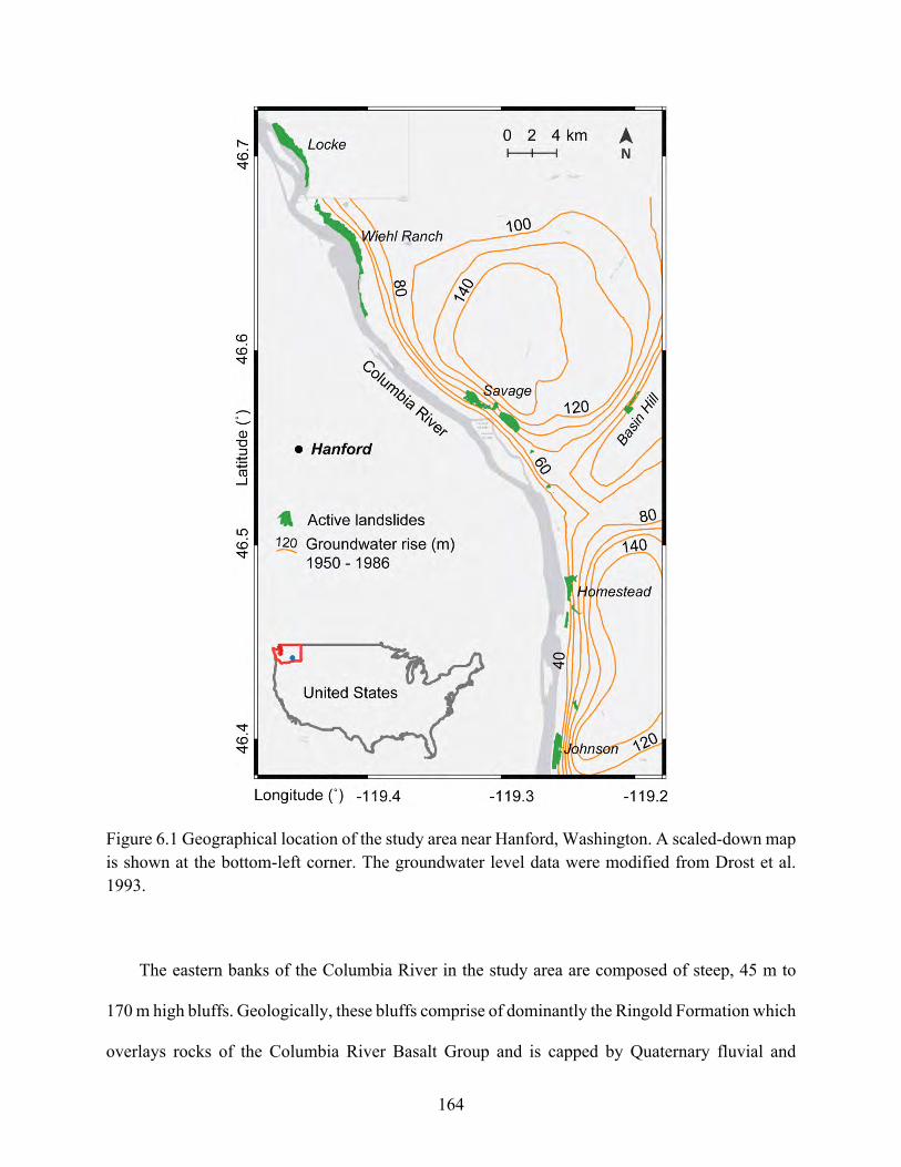
164
Figure 6.1 Geographical location of the study area near Hanford, Washington. A scaled-down map is shown at the bottom-left corner. The groundwater level data were modified from Drost et al. 1993.
The eastern banks of the Columbia River in the study area are composed of steep, 45 m to
170 m high bluffs. Geologically, these bluffs comprise of dominantly the Ringold Formation which
overlays rocks of the Columbia River Basalt Group and is capped by Quaternary fluvial and
165
windblown sediments (Schuster et al., 1989). The Ringold Formation is termed for the nearly
horizontal, soft rock layers (locally dipped towards the Columbia River by 1˚) composed of weakly
indurated claystone, siltstones, and sandstones near Hanford (Schuster et al., 1989). Mechanically,
the soft rocks of the Ringold Formation are relatively strong when dry yet becomes weak when
wetted. Laboratory tests of undisturbed soil samples from the bluff (Bareither et al., 2012) show
that saturating the soil sample decreases the friction angle from 32.9˚ to 19.8˚ and the cohesion
from 274 kPa to 46 kPa in the vertical orientation. Along the horizontal orientation, it reduces the
friction angle from 22.7˚ to 21˚ and the cohesion from 368 kPa to 16.7 kPa.
From 1950 to March 1983, excessive agricultural irrigation elevated the groundwater level of
the study area by 40 to 140 m (Figure 6.1) from unlined canal leakage and wastewater drainage
(Drost, 1993). In addition, the irrigation water vertically infiltrates into the farmland subsurface
and evolves into horizontal flows along the fine-grained, low-permeability layers to produce
extensive water seepage on the bluffs (Bjornstad and Peterson, 2019). Elevated basal pore pressure
and weakened soil shear strength together contributed to widespread landslide activities at the
steep bluffs along the Columbia River and other hillslopes in the study region (Figure 6.1).
6.3 Data and Methods
This investigation was aimed at mapping active landslides and measuring their time-series
displacements using satellite optical and radar images and the Interferometric Synthetic Aperture
Radar (InSAR) technique. Moreover, numerical modeling and topographical maps were
incorporated to decipher mechanisms of the contrasting post-failure slow and rapid motions of the
observed variable types of landslides.
166
6.3.1 Data
The Sentinel-1 SAR images from the ascending track A166 (January 2016 – September 2020)
and the descending track D42 (August 2015 – September 2020) were used to discover slow
landslides and measure their time-series displacements. Google Earth images from 1996 to 2020
were utilized to identify catastrophic landslides and measuring time-series motion of a fast
landslide. A 1924 topographical map and the National Elevation Datasets (USGS, 2021a) and a
2010 lidar DEM from Washington Department of Natural Resources were employed to produce
pre-landslide and/or post-landslide topography of selected landslides. Daily water level of the
Columbia River was obtained from a river gauge located immediately below the Priest Rapids
Dam (38 km upstream of the Locke landslide in Figure 6.2b) (USGS, 2021b). Daily precipitation
data of the study area were obtained from a meteorological station at the Saddle Mountain (18 km
west of the Locke landslide in Figure 6.2b) (WRCC, 2021). Groundwater records from 1964 to
1983 were collected at a well 1 km east of the Johnson landslide by U.S. Bureau of Reclamation.
(Figure 6.2b; Schuster et al., 1989).
6.3.2 Multitemporal InSAR Processing
SAR interferometry is a technique that utilizes the phase information in satellite radar images
to achieve displacement measurement of ground objects in millimeter-level accuracy (e.g., Ferretti
et al., 2007). A SAR interferogram is produced from two repeat-path SAR images that are usually
separated by several days. Multiple SAR interferograms spanning varied observation periods can
be used to generate time-series measurements of a ground target.
In this investigation, we utilized both ascending and descending Sentinel-1 SAR images from
2015 to 2020 to obtain InSAR time-series measurement of the target slow landslides. The National
Elevation Datasets (USGS, 2021a) covering the study area were used during SAR interferogram
167
generation from the GAMMA software (Werner et al., 2000), and the stratified tropospheric
artifacts associated with surface topography were removed before phase unwrapping. Stable, high-
coherence (coherence > 0.7) reference regions (300 m × 300 m) within 1 km distant from each
target landslide were selected to remove potential artifacts sourcing from regional soil moisture
changes and turbulent troposphere in the interferograms. The Sentinel-1 SAR images were multi-
looked using factors of 5×2 (range by azimuth) before interferometric processing, and the
generated interferograms were unwrapped with the minimum cost flow method (Costantini, 1998).
Measurement accuracy of each pixel in an individual SAR interferogram can be quantified from
the estimated coherence (Rodriguez and Martin, 1992):
σ =λ4.
41
267
(1 − *")*"
(6.1)
where 9 is the uncertainty of InSAR measurements, : the radar wavelength, 6 and 7 the window
sizes for the coherence estimation, and * the coherence.
Multitemporal InSAR processing was achieved by using a coherence-weighted small baseline
subset (SBAS) method (see details in Section 3.3.2 or Xu et al., 2020). We selected only
interferograms spanning the two closest dates for the time-series inversion and set the minimum
coherence threshold as 0.4, which consequently leads to a minimum measurement uncertainty of
~ 0.35 mm for the time-series displacements.
6.3.3 Forced Water Circulation on A Wavy Sliding Surface
Field and laboratory evidence shows that many clayey, slow-moving landslides deform with
dominant displacements (commonly > 70%) concentrated on the millimeters to centimeters thick
basal shear zones (Hutchinson, 1983; Skempton and Petley, 1968; Morgenstern and Tchalenko,
168
1968; Collin, 1846; Keefer and Johnson, 1983; Ter-Stepanian, 1965; Zaruba and Mencl, 1982;
Gould, 1960). Slow landslides commonly move in steady rates accompanied by very short periods
of acceleration and deceleration, and sustained acceleration resulting in rapid motion never occurs
(Keefer and Johnson, 1983; Baum and Johnson, 1993). The steady movements could be explained
using the forced pore fluid circulation (Baum and Johnson, 1993) on an irregular basal surface
which reduces basal pore pressure and obstructs downslope landslide movement (Figure 6.2).
Physically, it can be understood as that water is squeezed out of soil on upstream side of bumps
(; > 0) whereas sucked into swelling soil on downstream sides of bumps (; < 0). The forced
water circulation model simplifies slow landslides as a porous elastic solid sliding over a wavy,
impermeable, rigid surface with an average rate ?# along the x direction (Figure 6.2), and the stress
and pore water movement in the landslide materials are governed by four equations (Baum and
Johnson, 1993; Rice and Cleary, 1976):
AB##AC
+AB$#AE
+ *% sin I = 0(6.2)
AB$#AC
+AB$$AE
+ *% cos I = 0(6.3)
∇" MB## + B$$ +1 − 2N1 − N
OP = 0(6.4)
2QR(1 − N)
*&(1 − 2N)∇"(B## + B$$ + 2O) =
AAS(B## + B$$ + 2O)(6.5)
where B##, B$$, B$# are the stresses as shown in Figure 6.2. *% is the unit weight of the saturated
soils, I is the slope angle, N is the Poisson’s ratio for drained deformation, O is the pore-water
pressure, Q is the hydraulic conductivity, R is the shear modulus, and *& is the unit weight of
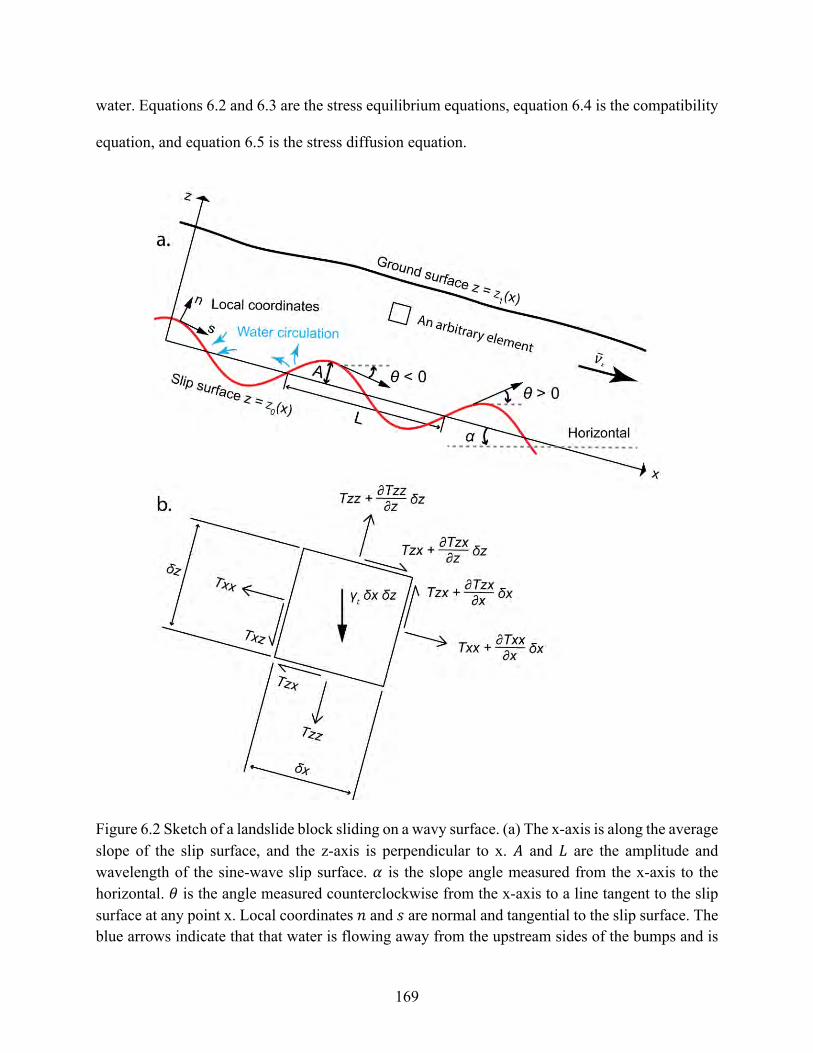
169
water. Equations 6.2 and 6.3 are the stress equilibrium equations, equation 6.4 is the compatibility
equation, and equation 6.5 is the stress diffusion equation.
Figure 6.2 Sketch of a landslide block sliding on a wavy surface. (a) The x-axis is along the average slope of the slip surface, and the z-axis is perpendicular to x. " and T are the amplitude and wavelength of the sine-wave slip surface. I is the slope angle measured from the x-axis to the horizontal. ; is the angle measured counterclockwise from the x-axis to a line tangent to the slip surface at any point x. Local coordinates U and V are normal and tangential to the slip surface. The blue arrows indicate that that water is flowing away from the upstream sides of the bumps and is
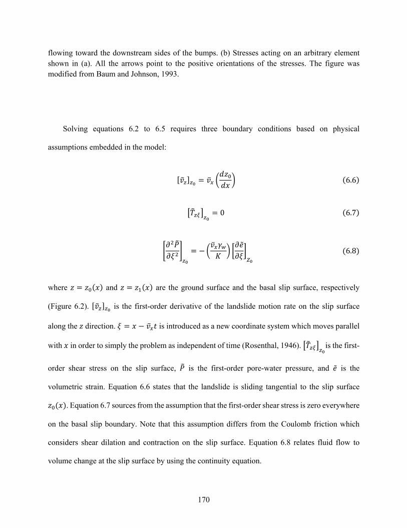
170
flowing toward the downstream sides of the bumps. (b) Stresses acting on an arbitrary element shown in (a). All the arrows point to the positive orientations of the stresses. The figure was modified from Baum and Johnson, 1993.
Solving equations 6.2 to 6.5 requires three boundary conditions based on physical
assumptions embedded in the model:
[?X$]$! = ?# MZE'ZC
P(6.6)
[B\$(]$!= 0(6.7)
_A"O\
A`"a$!= −M
?#*&Q
P bAcA`e)!(6.8)
where E = E'(C) and E = E*(C) are the ground surface and the basal slip surface, respectively
(Figure 6.2). [?X$]$! is the first-order derivative of the landslide motion rate on the slip surface
along the E direction. ` = C − ?#S is introduced as a new coordinate system which moves parallel
with C in order to simply the problem as independent of time (Rosenthal, 1946). [B\$(]$!is the first-
order shear stress on the slip surface, O\ is the first-order pore-water pressure, and c is the
volumetric strain. Equation 6.6 states that the landslide is sliding tangential to the slip surface
E'(C). Equation 6.7 sources from the assumption that the first-order shear stress is zero everywhere
on the basal slip boundary. Note that this assumption differs from the Coulomb friction which
considers shear dilation and contraction on the slip surface. Equation 6.8 relates fluid flow to
volume change at the slip surface by using the continuity equation.
171
Using the above three boundary conditions to solve equations 6.2 to 6.5 and drop several non-
significant high-order terms, the average resistance g which results from the slip surface roughness
and acts parallel to C can be obtained (Baum and Johnson, 1993):
g = −?#("h)"*&(1 − 2N)"
4Qh(1 − N)"(6.9)
where h = 2./T is the wave number, L is the wavelength of sinusoidal bumps on the slip surface,
"h, the product of the amplitude and the wave number, is the maximum local slope of the slip
surface with respect to C. Equation 6.9 shows that the sliding resistance g resulting from forced
water circulation increases linearly with the average landslide motion rate ?#. It would
consequently contribute to stopping slow landslides from infinite acceleration after the shearing
failure instigates.
6.4 Preliminary Results
6.4.1 Mapping Slow and Catastrophic Landslides
Using SAR interferograms from both the ascending Sentinel-1 track A166 and the descending
track D42 between August 2015 to September 2020 as well as satellite optical images from the
Google Earth between 1996 to 2020, we identified 12 concurrently active slow large landslide
complexes and 13 catastrophic landslides in the study region near Hanford, Washington (Figure
6.3). These identified landslides dominantly occurred at the bluffs along the eastern bank of the
Columbia River. Currently, active landslide regions (31.3 km) occupy 50.2 % of the eastern
Columbia River bank in the study region (62.1 km).
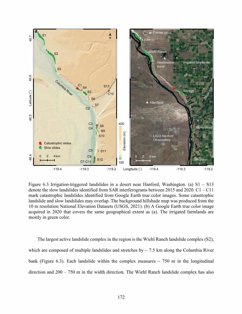
172
Figure 6.3 Irrigation-triggered landslides in a desert near Hanford, Washington. (a) S1 – S13 denote the slow landslides identified from SAR interferograms between 2015 and 2020. C1 – C11 mark catastrophic landslides identified from Google Earth true color images. Some catastrophic landslide and slow landslides may overlap. The background hillshade map was produced from the 10 m resolution National Elevation Datasets (USGS, 2021). (b) A Google Earth true color image acquired in 2020 that covers the same geographical extent as (a). The irrigated farmlands are mostly in green color.
The largest active landslide complex in the region is the Wiehl Ranch landslide complex (S2),
which are composed of multiple landslides and stretches by ~ 7.5 km along the Columbia River
bank (Figure 6.3). Each landslide within the complex measures ~ 750 m in the longitudinal
direction and 200 – 750 m in the width direction. The Wiehl Ranch landslide complex has also
173
been rapidly expanding south from 1996 to 2020 which potentially resulted from water infiltration
from the wastewater pond 4 km east of the landslide headscarp (Figure 6.3b). The largest
catastrophic runout landslide (C1) occurred near the Savage landslide complex in June 2017,
which inundated a 940 m by 830 m (length by width) region along the hillslope. The formed earth
flows remain active with slow motions by September 2020 (Figures 6.3 and 6.4). This also explains
the overlaps among polygons of the identified slow and catastrophic landslides in Figure 6.3.
Moreover, the 2020 true color image (Figure 6.3b) illustrates that vast farmlands in green colors
exist on the eastern side of the Columbia River where the active landslides reside. In contrast, the
dry lands in the western side of the Columbia River were not irrigated and did not include any
identified landslides.
Annual movement rates at different locations within a same landslide complex vary
significantly, which indicates that the landslide complexes are composed of multiple relatively
independent landslides moving towards the Columbia River. For example, the northernmost
section of the Locke landslide complex (S1) had a 3.3 cm/year Line-of-Sight (LOS) motion rate
between 2015 and 2020 from the ascending Sentinel-1 SAR images, whereas the central section
moved at 1.5 cm/year and some sections remained almost stable (Figure 6.4a). Similarly, the
Savage landslide complex (S5) experienced most deformation (2 – 3 cm/year along A166 LOS
direction) at the northernmost and the southernmost sections, whereas the central section only
moved at 0.4 cm/year (Figure 6.4a). The individual landslides within a complex are also
distinguishable from their separate, curve-shaped headscarps ((Figure 6.4). The identified large
catastrophic landslides (e.g., C1, C6, C12) were commonly initiated at their steep headscarps
beside the irrigated farmlands (Figure 6.4b) and were instigated in irrigation seasons (April to
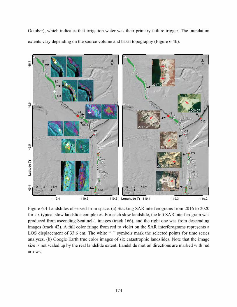
174
October), which indicates that irrigation water was their primary failure trigger. The inundation
extents vary depending on the source volume and basal topography (Figure 6.4b).
Figure 6.4 Landslides observed from space. (a) Stacking SAR interferograms from 2016 to 2020 for six typical slow landslide complexes. For each slow landslide, the left SAR interferogram was produced from ascending Sentinel-1 images (track 166), and the right one was from descending images (track 42). A full color fringe from red to violet on the SAR interferograms represents a LOS displacement of 33.6 cm. The white “+” symbols mark the selected points for time series analyses. (b) Google Earth true color images of six catastrophic landslides. Note that the image size is not scaled up by the real landslide extent. Landslide motion directions are marked with red arrows.
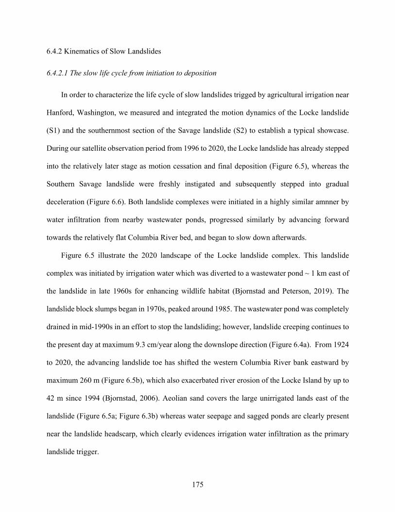
175
6.4.2 Kinematics of Slow Landslides
6.4.2.1 The slow life cycle from initiation to deposition
In order to characterize the life cycle of slow landslides trigged by agricultural irrigation near
Hanford, Washington, we measured and integrated the motion dynamics of the Locke landslide
(S1) and the southernmost section of the Savage landslide (S2) to establish a typical showcase.
During our satellite observation period from 1996 to 2020, the Locke landslide has already stepped
into the relatively later stage as motion cessation and final deposition (Figure 6.5), whereas the
Southern Savage landslide were freshly instigated and subsequently stepped into gradual
deceleration (Figure 6.6). Both landslide complexes were initiated in a highly similar amnner by
water infiltration from nearby wastewater ponds, progressed similarly by advancing forward
towards the relatively flat Columbia River bed, and began to slow down afterwards.
Figure 6.5 illustrate the 2020 landscape of the Locke landslide complex. This landslide
complex was initiated by irrigation water which was diverted to a wastewater pond ~ 1 km east of
the landslide in late 1960s for enhancing wildlife habitat (Bjornstad and Peterson, 2019). The
landslide block slumps began in 1970s, peaked around 1985. The wastewater pond was completely
drained in mid-1990s in an effort to stop the landsliding; however, landslide creeping continues to
the present day at maximum 9.3 cm/year along the downslope direction (Figure 6.4a). From 1924
to 2020, the advancing landslide toe has shifted the western Columbia River bank eastward by
maximum 260 m (Figure 6.5b), which also exacerbated river erosion of the Locke Island by up to
42 m since 1994 (Bjornstad, 2006). Aeolian sand covers the large unirrigated lands east of the
landslide (Figure 6.5a; Figure 6.3b) whereas water seepage and sagged ponds are clearly present
near the landslide headscarp, which clearly evidences irrigation water infiltration as the primary
landslide trigger.
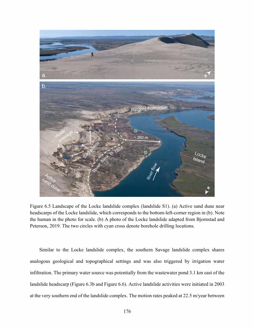
176
Figure 6.5 Landscape of the Locke landslide complex (landslide S1). (a) Active sand dune near headscarps of the Locke landslide, which corresponds to the bottom-left-corner region in (b). Note the human in the photo for scale. (b) A photo of the Locke landslide adapted from Bjornstad and Peterson, 2019. The two circles with cyan cross denote borehole drilling locations.
Similar to the Locke landslide complex, the southern Savage landslide complex shares
analogous geological and topographical settings and was also triggered by irrigation water
infiltration. The primary water source was potentially from the wastewater pond 3.1 km east of the
landslide headscarp (Figure 6.3b and Figure 6.6). Active landslide activities were initiated in 2003
at the very southern end of the landslide complex. The motion rates peaked at 22.5 m/year between
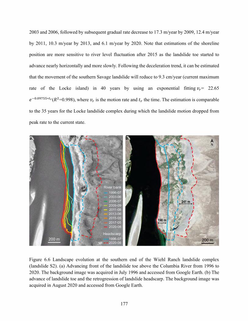
177
2003 and 2006, followed by subsequent gradual rate decrease to 17.3 m/year by 2009, 12.4 m/year
by 2011, 10.3 m/year by 2013, and 6.1 m/year by 2020. Note that estimations of the shoreline
position are more sensitive to river level fluctuation after 2015 as the landslide toe started to
advance nearly horizontally and more slowly. Following the deceleration trend, it can be estimated
that the movement of the southern Savage landslide will reduce to 9.3 cm/year (current maximum
rate of the Locke island) in 40 years by using an exponential fitting?+= 22.65
c,'.'./00∗2"(g"=0.998), where ?+ is the motion rate and S+ the time. The estimation is comparable
to the 35 years for the Locke landslide complex during which the landslide motion dropped from
peak rate to the current state.
Figure 6.6 Landscape evolution at the southern end of the Wiehl Ranch landslide complex (landslide S2). (a) Advancing front of the landslide toe above the Columbia River from 1996 to 2020. The background image was acquired in July 1996 and accessed from Google Earth. (b) The advance of landslide toe and the retrogression of landslide headscarp. The background image was acquired in August 2020 and accessed from Google Earth.
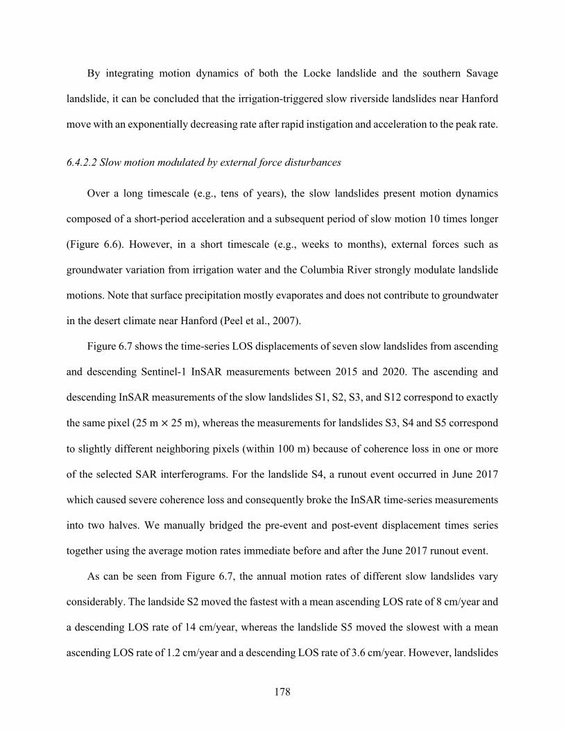
178
By integrating motion dynamics of both the Locke landslide and the southern Savage
landslide, it can be concluded that the irrigation-triggered slow riverside landslides near Hanford
move with an exponentially decreasing rate after rapid instigation and acceleration to the peak rate.
6.4.2.2 Slow motion modulated by external force disturbances
Over a long timescale (e.g., tens of years), the slow landslides present motion dynamics
composed of a short-period acceleration and a subsequent period of slow motion 10 times longer
(Figure 6.6). However, in a short timescale (e.g., weeks to months), external forces such as
groundwater variation from irrigation water and the Columbia River strongly modulate landslide
motions. Note that surface precipitation mostly evaporates and does not contribute to groundwater
in the desert climate near Hanford (Peel et al., 2007).
Figure 6.7 shows the time-series LOS displacements of seven slow landslides from ascending
and descending Sentinel-1 InSAR measurements between 2015 and 2020. The ascending and
descending InSAR measurements of the slow landslides S1, S2, S3, and S12 correspond to exactly
the same pixel (25 m × 25 m), whereas the measurements for landslides S3, S4 and S5 correspond
to slightly different neighboring pixels (within 100 m) because of coherence loss in one or more
of the selected SAR interferograms. For the landslide S4, a runout event occurred in June 2017
which caused severe coherence loss and consequently broke the InSAR time-series measurements
into two halves. We manually bridged the pre-event and post-event displacement times series
together using the average motion rates immediate before and after the June 2017 runout event.
As can be seen from Figure 6.7, the annual motion rates of different slow landslides vary
considerably. The landside S2 moved the fastest with a mean ascending LOS rate of 8 cm/year and
a descending LOS rate of 14 cm/year, whereas the landslide S5 moved the slowest with a mean
ascending LOS rate of 1.2 cm/year and a descending LOS rate of 3.6 cm/year. However, landslides
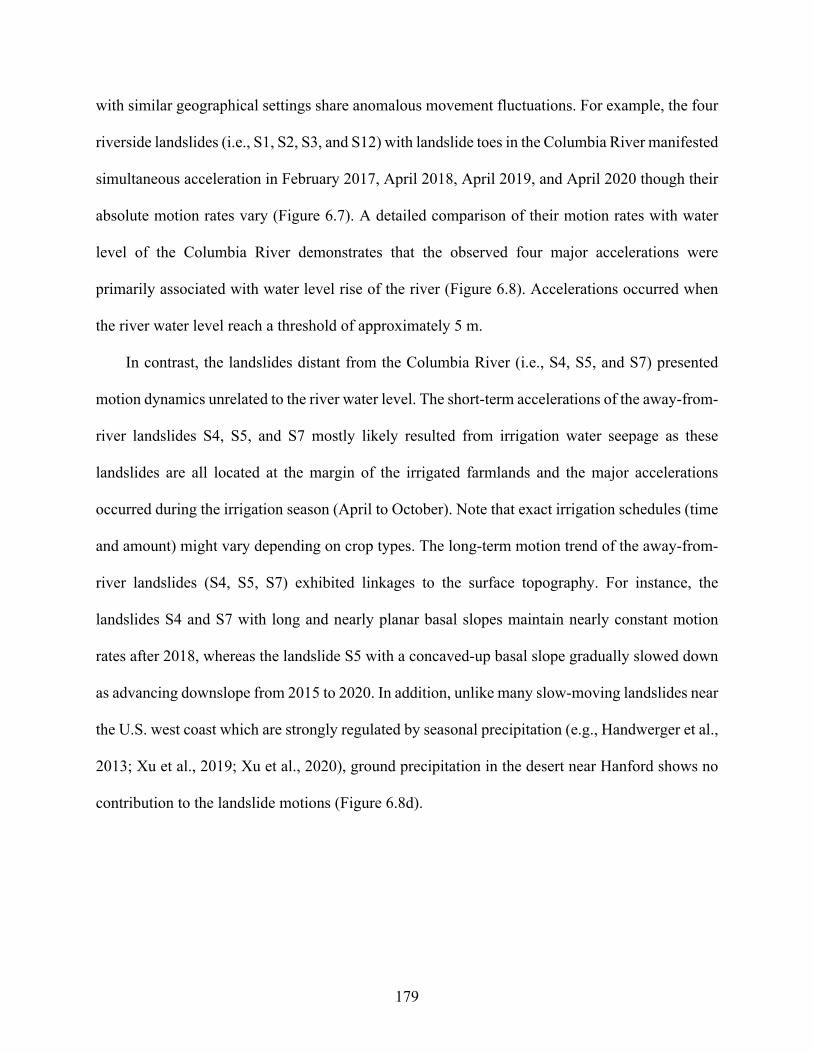
179
with similar geographical settings share anomalous movement fluctuations. For example, the four
riverside landslides (i.e., S1, S2, S3, and S12) with landslide toes in the Columbia River manifested
simultaneous acceleration in February 2017, April 2018, April 2019, and April 2020 though their
absolute motion rates vary (Figure 6.7). A detailed comparison of their motion rates with water
level of the Columbia River demonstrates that the observed four major accelerations were
primarily associated with water level rise of the river (Figure 6.8). Accelerations occurred when
the river water level reach a threshold of approximately 5 m.
In contrast, the landslides distant from the Columbia River (i.e., S4, S5, and S7) presented
motion dynamics unrelated to the river water level. The short-term accelerations of the away-from-
river landslides S4, S5, and S7 mostly likely resulted from irrigation water seepage as these
landslides are all located at the margin of the irrigated farmlands and the major accelerations
occurred during the irrigation season (April to October). Note that exact irrigation schedules (time
and amount) might vary depending on crop types. The long-term motion trend of the away-from-
river landslides (S4, S5, S7) exhibited linkages to the surface topography. For instance, the
landslides S4 and S7 with long and nearly planar basal slopes maintain nearly constant motion
rates after 2018, whereas the landslide S5 with a concaved-up basal slope gradually slowed down
as advancing downslope from 2015 to 2020. In addition, unlike many slow-moving landslides near
the U.S. west coast which are strongly regulated by seasonal precipitation (e.g., Handwerger et al.,
2013; Xu et al., 2019; Xu et al., 2020), ground precipitation in the desert near Hanford shows no
contribution to the landslide motions (Figure 6.8d).
180
Figure 6.7 Time-series displacements of seven slow-moving landslides between July 2015 to October 2020 from Sentinel-1 InSAR measurements. Geographical locations of the selected
181
measurement points for the landslides are depicted in Figure 6.3. (a), (b), (c), and (g) show displacement measurements of a same geographical point from ascending (A166) and descending (D42) SAR data for each individual landslide. (d), (e), and (f) show measurements at slightly different locations (within 100 m) on a landslide from ascending and descending data because of coherence loss in one of the SAR datasets. Positive LOS displacements denote distance shortening between ground targets and the satellite.
Figure 6.8 Relationship of landslide movement with regard to rainfall and groundwater level for the riverside slow landslides S1 and S2. (a) Orange circles denote LOS displacements of the landslide S2 from the Sentinel-1 descending track D42. The green polyline shows the corresponding movement velocity as scaled by the green labeling on the right. (b) Movement measurements of the landslide S1, with same labeling rules as (a). (c) Water level of the Columbia
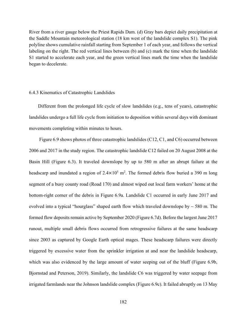
182
River from a river gauge below the Priest Rapids Dam. (d) Gray bars depict daily precipitation at the Saddle Mountain meteorological station (18 km west of the landslide complex S1). The pink polyline shows cumulative rainfall starting from September 1 of each year, and follows the vertical labeling on the right. The red vertical lines between (b) and (c) mark the time when the landslide S1 started to accelerate each year, and the green vertical lines mark the time when the landslide began to decelerate.
6.4.3 Kinematics of Catastrophic Landslides
Different from the prolonged life cycle of slow landslides (e.g., tens of years), catastrophic
landslides undergo a full life cycle from initiation to deposition within several days with dominant
movements completing within minutes to hours.
Figure 6.9 shows photos of three catastrophic landslides (C12, C1, and C6) occurred between
2006 and 2017 in the study region. The catastrophic landslide C12 failed on 20 August 2008 at the
Basin Hill (Figure 6.3). It traveled downslope by up to 580 m after an abrupt failure at the
headscarp and inundated a region of 2.4×10⁵ m2. The formed debris flow buried a 390 m long
segment of a busy county road (Road 170) and almost wiped out local farm workers’ home at the
bottom-right corner of the debris in Figure 6.9a. Landslide C1 occurred in early June 2017 and
evolved into a typical “hourglass” shaped earth flow which traveled downslope by ~ 580 m. The
formed flow deposits remain active by September 2020 (Figure 6.7d). Before the largest June 2017
runout, multiple small debris flows occurred from retrogressive failures at the same headscarp
since 2003 as captured by Google Earth optical mages. These headscarp failures were directly
triggered by excessive water from the sprinkler irrigation at and near the landslide headscarp,
which was also evidenced by the large amount of water seeping out of the bluff (Figure 6.9b,
Bjornstad and Peterson, 2019). Similarly, the landslide C6 was triggered by water seepage from
irrigated farmlands near the Johnson landslide complex (Figure 6.9c). It failed abruptly on 13 May
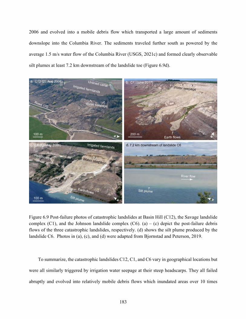
183
2006 and evolved into a mobile debris flow which transported a large amount of sediments
downslope into the Columbia River. The sediments traveled further south as powered by the
average 1.5 m/s water flow of the Columbia River (USGS, 2021c) and formed clearly observable
silt plumes at least 7.2 km downstream of the landslide toe (Figure 6.9d).
Figure 6.9 Post-failure photos of catastrophic landslides at Basin Hill (C12), the Savage landslide complex (C1), and the Johnson landslide complex (C6). (a) – (c) depict the post-failure debris flows of the three catastrophic landslides, respectively. (d) shows the silt plume produced by the landslide C6. Photos in (a), (c), and (d) were adapted from Bjornstad and Peterson, 2019.
To summarize, the catastrophic landslides C12, C1, and C6 vary in geographical locations but
were all similarly triggered by irrigation water seepage at their steep headscarps. They all failed
abruptly and evolved into relatively mobile debris flows which inundated areas over 10 times
184
larger than the landslide source. Compared to the prolonged life cycle of slow landslides, these
catastrophic landslides completed the process from initiation to deposition within one day
(potentially in a few hours but no temporally dense observations are available for the verification).
6.4.4 Landslide Motion Regulated by Basal Topography
6.4.4.1 Basal topography regulates slow landslides by forced water circulation
Here we take the Loke landslide complex as a typical example to investigate the potential
regulation of slow landslide motions by forced water circulation on a wavy surface. As introduced
in Section 6.4.2.1, the Locke landslide complex was initiated by water infiltration from a
wastewater pond which was later completely drained in mid-1990s. Ground precipitation is also
not a factor that contributes to groundwater in the desert climate (Peel et al., 2007). Hence, the
groundwater level within the Locke landslide complex was dominantly controlled by water level
of the Columbia River where 44% of the landslide body resides (approximately 250 m long). This
was also verified by piezometer measurements from ten boreholes drilled on and near the landslide
complex in 1998 and 1999 (Bennett et al., 2002). Four boreholes were drilled in 1998 along a
north-south orientated line approximately 500 m east of the landslide headscarps, four were drilled
much farther east of the landslide complex (over 1 km) in 1998, and two others were drilled on the
landslide toe (Figure 6.5b). The borehole piezometer measurements suggest that the far east side
of the landslide were completely dry from 1988 to 2002, whereas the groundwater level within
500 m east of the landslide complex was almost the same as the Columbia River surface at 114.6
m above sea level. Moreover, the borehole drilling revealed that landslide thicknesses at the toe
were 16.6 m (the northern one) and 14.8 m (the southern one), respectively (Bennett et al., 2002).
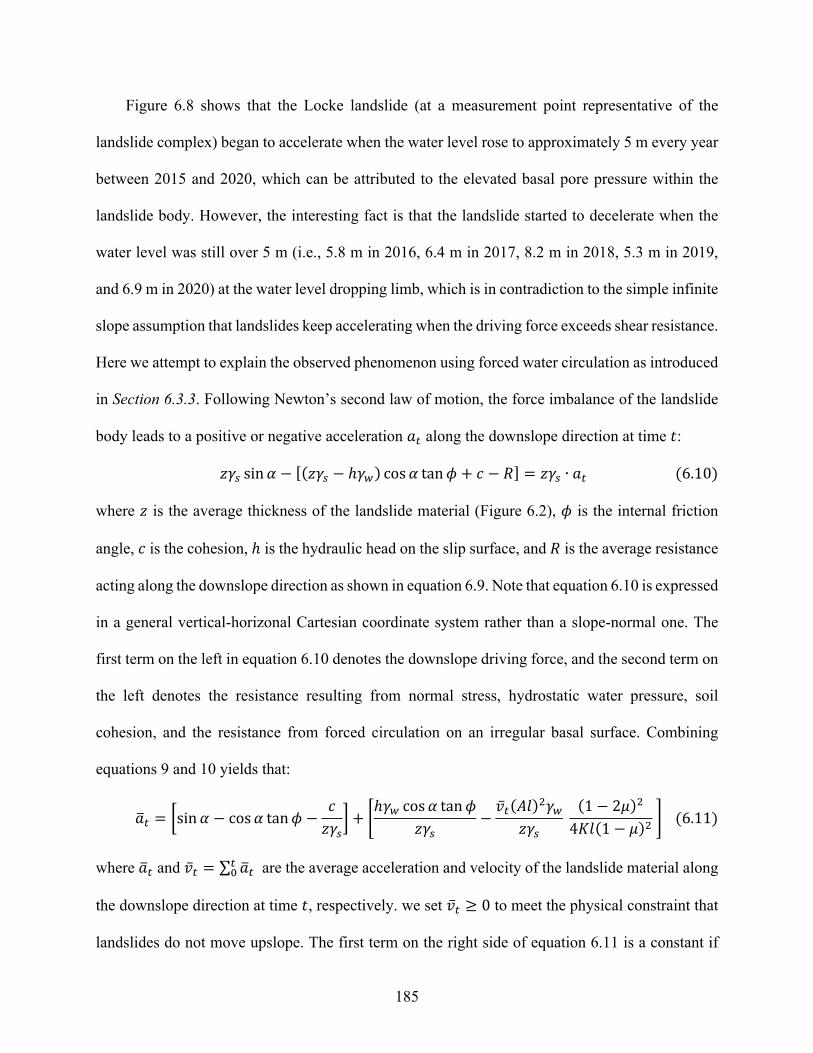
185
Figure 6.8 shows that the Locke landslide (at a measurement point representative of the
landslide complex) began to accelerate when the water level rose to approximately 5 m every year
between 2015 and 2020, which can be attributed to the elevated basal pore pressure within the
landslide body. However, the interesting fact is that the landslide started to decelerate when the
water level was still over 5 m (i.e., 5.8 m in 2016, 6.4 m in 2017, 8.2 m in 2018, 5.3 m in 2019,
and 6.9 m in 2020) at the water level dropping limb, which is in contradiction to the simple infinite
slope assumption that landslides keep accelerating when the driving force exceeds shear resistance.
Here we attempt to explain the observed phenomenon using forced water circulation as introduced
in Section 6.3.3. Following Newton’s second law of motion, the force imbalance of the landslide
body leads to a positive or negative acceleration k2 along the downslope direction at time S:
E*% sin I − [(E*% − ℎ*&) cos I tano + p − g] = E*% ∙ k2(6.10)
where E is the average thickness of the landslide material (Figure 6.2), o is the internal friction
angle, p is the cohesion, ℎ is the hydraulic head on the slip surface, and g is the average resistance
acting along the downslope direction as shown in equation 6.9. Note that equation 6.10 is expressed
in a general vertical-horizonal Cartesian coordinate system rather than a slope-normal one. The
first term on the left in equation 6.10 denotes the downslope driving force, and the second term on
the left denotes the resistance resulting from normal stress, hydrostatic water pressure, soil
cohesion, and the resistance from forced circulation on an irregular basal surface. Combining
equations 9 and 10 yields that:
kr2 = bsin I − cos I tano −pE*%
e + _ℎ*& cos I tano
E*%−?2("h)"*&
E*%(1 − 2N)"
4Qh(1 − N)"a(6.11)
where kr2 and ?2 = ∑ kr22' are the average acceleration and velocity of the landslide material along
the downslope direction at time S, respectively. we set ?2 ≥ 0 to meet the physical constraint that
landslides do not move upslope. The first term on the right side of equation 6.11 is a constant if
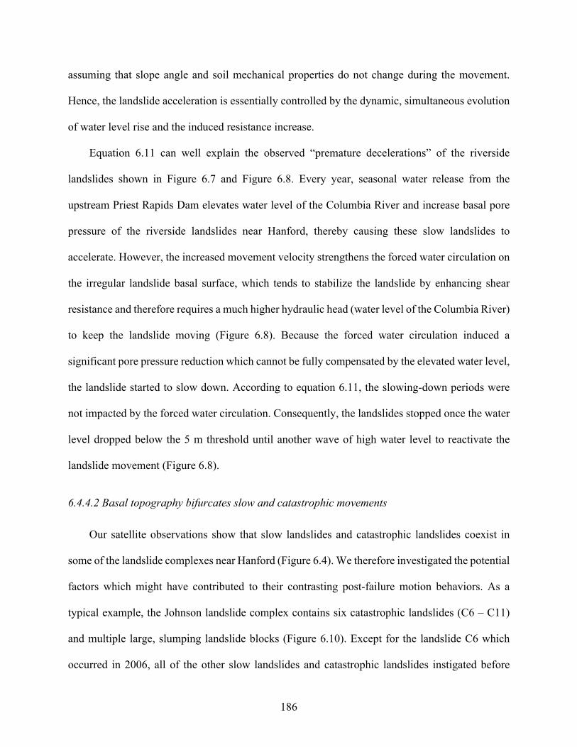
186
assuming that slope angle and soil mechanical properties do not change during the movement.
Hence, the landslide acceleration is essentially controlled by the dynamic, simultaneous evolution
of water level rise and the induced resistance increase.
Equation 6.11 can well explain the observed “premature decelerations” of the riverside
landslides shown in Figure 6.7 and Figure 6.8. Every year, seasonal water release from the
upstream Priest Rapids Dam elevates water level of the Columbia River and increase basal pore
pressure of the riverside landslides near Hanford, thereby causing these slow landslides to
accelerate. However, the increased movement velocity strengthens the forced water circulation on
the irregular landslide basal surface, which tends to stabilize the landslide by enhancing shear
resistance and therefore requires a much higher hydraulic head (water level of the Columbia River)
to keep the landslide moving (Figure 6.8). Because the forced water circulation induced a
significant pore pressure reduction which cannot be fully compensated by the elevated water level,
the landslide started to slow down. According to equation 6.11, the slowing-down periods were
not impacted by the forced water circulation. Consequently, the landslides stopped once the water
level dropped below the 5 m threshold until another wave of high water level to reactivate the
landslide movement (Figure 6.8).
6.4.4.2 Basal topography bifurcates slow and catastrophic movements
Our satellite observations show that slow landslides and catastrophic landslides coexist in
some of the landslide complexes near Hanford (Figure 6.4). We therefore investigated the potential
factors which might have contributed to their contrasting post-failure motion behaviors. As a
typical example, the Johnson landslide complex contains six catastrophic landslides (C6 – C11)
and multiple large, slumping landslide blocks (Figure 6.10). Except for the landslide C6 which
occurred in 2006, all of the other slow landslides and catastrophic landslides instigated before
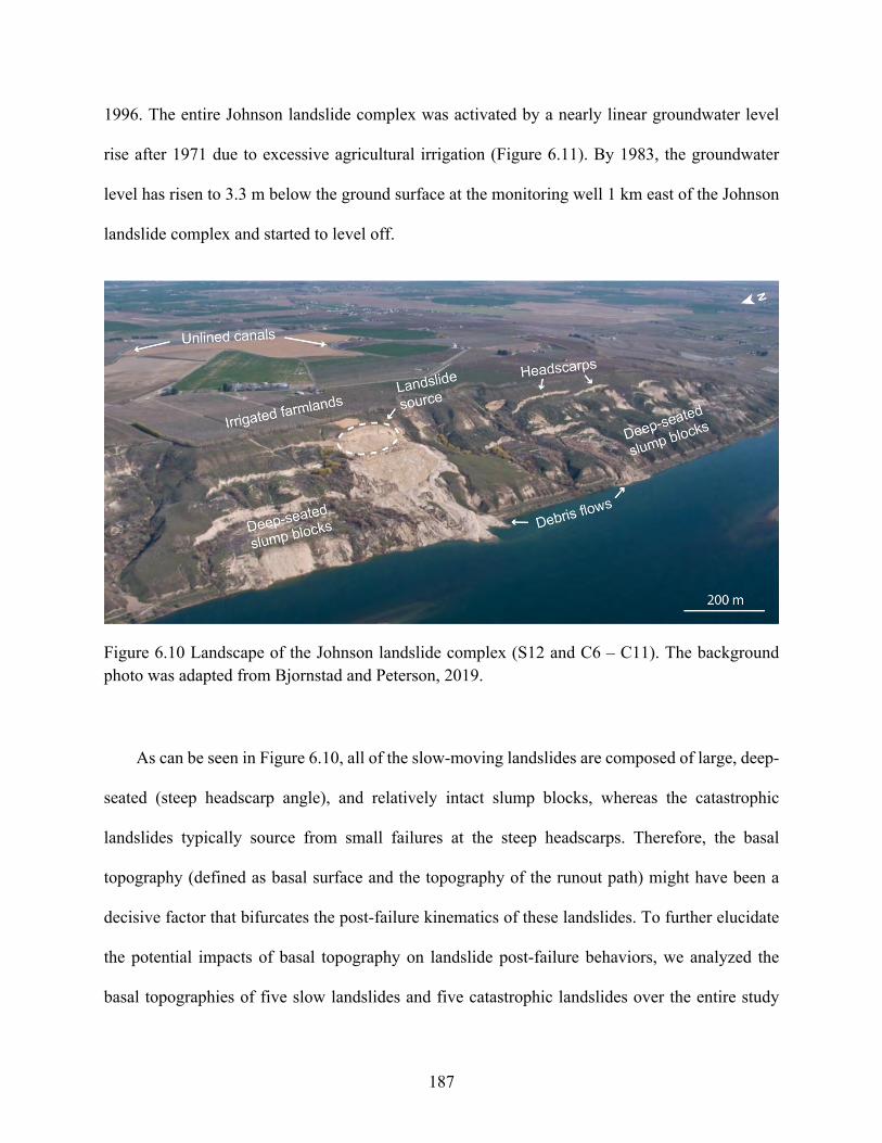
187
1996. The entire Johnson landslide complex was activated by a nearly linear groundwater level
rise after 1971 due to excessive agricultural irrigation (Figure 6.11). By 1983, the groundwater
level has risen to 3.3 m below the ground surface at the monitoring well 1 km east of the Johnson
landslide complex and started to level off.
Figure 6.10 Landscape of the Johnson landslide complex (S12 and C6 – C11). The background photo was adapted from Bjornstad and Peterson, 2019.
As can be seen in Figure 6.10, all of the slow-moving landslides are composed of large, deep-
seated (steep headscarp angle), and relatively intact slump blocks, whereas the catastrophic
landslides typically source from small failures at the steep headscarps. Therefore, the basal
topography (defined as basal surface and the topography of the runout path) might have been a
decisive factor that bifurcates the post-failure kinematics of these landslides. To further elucidate
the potential impacts of basal topography on landslide post-failure behaviors, we analyzed the
basal topographies of five slow landslides and five catastrophic landslides over the entire study
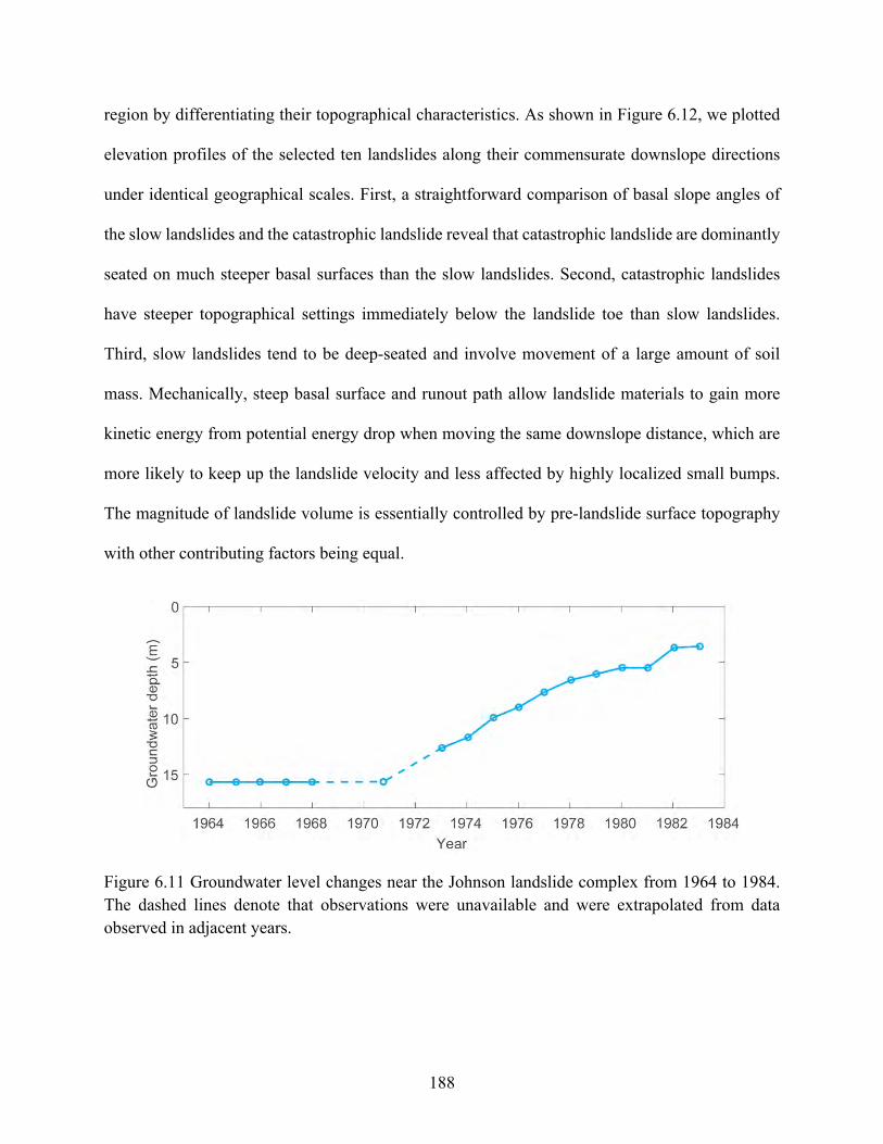
188
region by differentiating their topographical characteristics. As shown in Figure 6.12, we plotted
elevation profiles of the selected ten landslides along their commensurate downslope directions
under identical geographical scales. First, a straightforward comparison of basal slope angles of
the slow landslides and the catastrophic landslide reveal that catastrophic landslide are dominantly
seated on much steeper basal surfaces than the slow landslides. Second, catastrophic landslides
have steeper topographical settings immediately below the landslide toe than slow landslides.
Third, slow landslides tend to be deep-seated and involve movement of a large amount of soil
mass. Mechanically, steep basal surface and runout path allow landslide materials to gain more
kinetic energy from potential energy drop when moving the same downslope distance, which are
more likely to keep up the landslide velocity and less affected by highly localized small bumps.
The magnitude of landslide volume is essentially controlled by pre-landslide surface topography
with other contributing factors being equal.
Figure 6.11 Groundwater level changes near the Johnson landslide complex from 1964 to 1984. The dashed lines denote that observations were unavailable and were extrapolated from data observed in adjacent years.
189
Figure 6.12 Comparison between basal topography of slow landslides and catastrophic landslides near Hanford. Pre-slide topography of the three transects at landslide complex S1 were obtained from USGS topographical maps in 1924. Post-slide topography of the three transects were from lidar DEM acquired in 2010. Surface topography of other landslides are obtained from either the 2010 lidar DEM or the National Elevation Datasets (USGS, 2021). The headscarp location of each landslide was used as the reference point (x=0, y=0) for each panel, and the absolute elevation of the headscarp above sea level was given in the top-right corner of each panel.
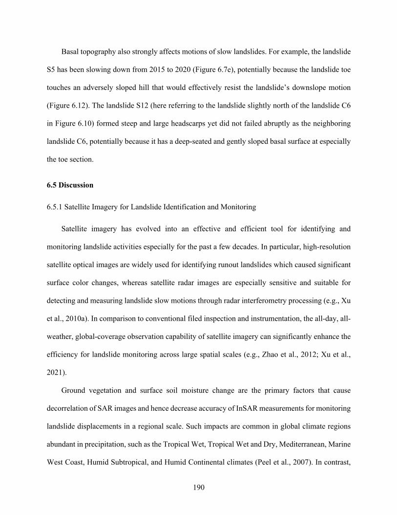
190
Basal topography also strongly affects motions of slow landslides. For example, the landslide
S5 has been slowing down from 2015 to 2020 (Figure 6.7e), potentially because the landslide toe
touches an adversely sloped hill that would effectively resist the landslide’s downslope motion
(Figure 6.12). The landslide S12 (here referring to the landslide slightly north of the landslide C6
in Figure 6.10) formed steep and large headscarps yet did not failed abruptly as the neighboring
landslide C6, potentially because it has a deep-seated and gently sloped basal surface at especially
the toe section.
6.5 Discussion
6.5.1 Satellite Imagery for Landslide Identification and Monitoring
Satellite imagery has evolved into an effective and efficient tool for identifying and
monitoring landslide activities especially for the past a few decades. In particular, high-resolution
satellite optical images are widely used for identifying runout landslides which caused significant
surface color changes, whereas satellite radar images are especially sensitive and suitable for
detecting and measuring landslide slow motions through radar interferometry processing (e.g., Xu
et al., 2010a). In comparison to conventional filed inspection and instrumentation, the all-day, all-
weather, global-coverage observation capability of satellite imagery can significantly enhance the
efficiency for landslide monitoring across large spatial scales (e.g., Zhao et al., 2012; Xu et al.,
2021).
Ground vegetation and surface soil moisture change are the primary factors that cause
decorrelation of SAR images and hence decrease accuracy of InSAR measurements for monitoring
landslide displacements in a regional scale. Such impacts are common in global climate regions
abundant in precipitation, such as the Tropical Wet, Tropical Wet and Dry, Mediterranean, Marine
West Coast, Humid Subtropical, and Humid Continental climates (Peel et al., 2007). In contrast,
191
InSAR measurements are less affected in the Semiarid or Desert climates due to the lack of
precipitation and rain clouds. Consequently, the arid region near Hanford in this study offered a
great opportunity for obtaining accurate InSAR measurements to characterize the landslide
movements. Moreover, the diverse types of landslides occurred near Hanford, Washington further
allowed the possibility to decipher impacts of other factors such as topography through mutual
comparisons by naturally excluding the influence of precipitation.
6.5.2 Human-Induced Landslides and Potential Prevention Measures
Landslides are a natural geomorphic process driven by gravity (Highland and Bobrowsky,
2008); however, recent decades have witnessed increasingly frequent landslide activities resulting
from global climate change and expanding anthropogenic activities (Gariano and Guzzetti, 2016;
Froude and Petley, 2018). Urban expansion, underground and surface mining, road and reservoir
construction, and irrigation farming are typical human activities that have caused numerous
landslides worldwide in the latest decades (Froude and Petley, 2018). In particular, intensive
irrigation farming which gained increased popularity in semiarid and arid regions since 1950s has
brought in considerable unexpected landslide problems besides the expected agricultural
production (Garcia-Chevesich et al., 2021). Moreover, seasonal water release from dammed rivers
and reservoirs which support the irrigation systems significantly controls the dynamics of riverside
landslides. Widespread landslide activities exacerbate soil erosion and farmland loss, transport
sediments to streams harming aquatic lives, and endanger life and property safety of local
residents. However, irrigation-induced landslide activities could be largely reduced with improved
irrigation measures.
We found in this investigation that landslides in the Washington desert near Hanford were
primarily triggered by excessive irrigation water which was not fully absorbed by crops and
192
therefore infiltrated into the subsurface layers. Water leakage from unlined canal and wastewater
ponds is another major factor that triggered landslides distant from the irrigated landslides.
Consequently, practicing efficient crop irrigation using controlled sprinkler systems is a potential
way to save water and reduce irrigation-induced landslide activities. Furthermore, canal lining
could be an effective measure to prevent water leakage and therefore the triggered landslides.
6.5.3 Implications of Basal Topography Control on Landslide Behaviors
Landslides initiate from basal shearing failure and may present diverse motion dynamics at
the post-failure stage. Deciphering what impacts landslide post-failure mobility could offer critical
understanding for mitigating life and property loss from a highly mobile landslide. In this study,
we found that basal topography exerts fundamental controls on landslide kinematics in three
distinct ways. First, an irregular basal slip surface could produce significant resistance through
forced water circulation to obstruct slow landslide motion after failures instigate on a relatively
gentle slope. Second, steep basal surface and runout path are more likely to produce catastrophic
landslides due to the rapid kinetic energy gain from potential energy drop during the downslope
movement. Landslide blocks breaking apart and forming debris flows under large deformation are
another potential factor to enhance the landslide mobility. Third, slow landslides could source from
debris deposits from a previous catastrophic landslide, and the dynamics of their slow motions are
strongly regulated by the basal topography in particularly the toe section. These fundamental
controls on landslide motion from basal topography apply to not only the irrigation-induced
landslides, but also many other slow and catastrophic landslides around the globe.
193
6.6 Conclusions
Landslides in the dry climate triggered by agricultural irrigation is a typical type of human-
induced geohazard. Monitoring the dynamics of these landslides and decipher their kinematic
controls are essential for understanding and reducing their potential hazards. In this investigation,
we utilized both satellite optical and radar imagery to discover both slow and catastrophic
landslides from 1996 to 2020 in a Washington desert near Hanford.
We retrieved the time-series displacement of seven slow landslides in the study region using
radar interferometry of both ascending and descending Sentinel-1 SAR images between 2015 and
2020. Our analyses reveal that the riverside landslides were triggered by agricultural irrigation yet
were strongly regulated by water level variation of the Columbia River where the landslide toes
reside. Moreover, the seasonal instigation and cessation of the riverside landslides were not
controlled by a single fix threshold of groundwater level, which can be explained by the forced
water circulation on an irregular slip surface where accelerated landslide velocity enhances basal
resistance and in turn contributes to slowing down the landslide movement. By integrating of
satellite observations of two highly similar irrigation-triggered slow landslides, we revealed the
prolonged life cycle of a typical slow landslide in the study region: a rapid acceleration to the peak
rate within 3 years followed by slow decelerations with exponentially decreasing rates for about
40 years.
We further investigated how basal topography could bifurcate the identified slow landslides
and catastrophic landslides. By comparing longitudinal topographical profiles of five typical slow
landslides and five catastrophic landslides in the study region, we found that steep basal slip
surface and runout path are more likely to produce catastrophic landslides with a long runout

194
distance, whereas gentle surface and basal slopes at particularly the toe region tend to produce
deep-seated, slow landslides.
Our findings in this study could contribute to understanding and mitigation of irrigation-
induced landslide around the globe. Moreover, the impacts of basal topography on landslide post-
failure kinematics are widely applicable to many slow and catastrophic landslides globally for
future hazard mitigation.
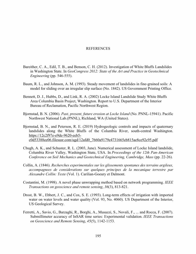
195
REFERENCES
Bareither, C. A., Edil, T. B., and Benson, C. H. (2012). Investigation of White Bluffs Landslides in Washington State. In GeoCongress 2012: State of the Art and Practice in Geotechnical Engineering (pp. 546-555).
Baum, R. L., and Johnson, A. M. (1993). Steady movement of landslides in fine-grained soils: A model for sliding over an irregular slip surface (No. 1842). US Government Printing Office.
Bennett, D. J., Hubbs, D., and Link, R. A. (2002) Locke Island Landslide Study White Bluffs Area Columbia Basin Project, Washington. Report to U.S. Department of the Interior Bureau of Reclamation, Pacific Northwest Region.
Bjornstad, B. N. (2006). Past, present, future erosion at Locke Island (No. PNNL-15941). Pacific Northwest National Lab.(PNNL), Richland, WA (United States).
Bjornstad, B. N., and Peterson, R. E. (2019) Hydrogeologic controls and impacts of quaternary landslides along the White Bluffs of the Columbia River, south-central Washington. https://12c2f97e-e9de-9620-eeb5-c0d53388ee06.filesusr.com/ugd/12afd0_7660a9179e4731665eb815ae8ce92c95.pdf
Chugh, A. K., and Schuster, R. L. (2003, June). Numerical assessment of Locke Island landslide, Columbia River Valley, Washington State, USA. In Proceedings of the 12th Pan-American Conference on Soil Mechanics and Geotechnical Engineering, Cambridge, Mass (pp. 22-26).
Collin, A. (1846). Recherches experimentales sur les glissements spontanes des terrains argileux, accompagnees de considerations sur quelques principes de la mecanique terrestre par Alexandre Collin: Texte (Vol. 1). Carilian-Goeury et Dalmont.
Costantini, M. (1998). A novel phase unwrapping method based on network programming. IEEE Transactions on geoscience and remote sensing, 36(3), 813-821.
Drost, B. W., Ebbert, J. C., and Cox, S. E. (1993). Long-term effects of irrigation with imported water on water levels and water quality (Vol. 93, No. 4060). US Department of the Interior, US Geological Survey.
Ferretti, A., Savio, G., Barzaghi, R., Borghi, A., Musazzi, S., Novali, F., ... and Rocca, F. (2007). Submillimeter accuracy of InSAR time series: Experimental validation. IEEE Transactions on Geoscience and Remote Sensing, 45(5), 1142-1153.
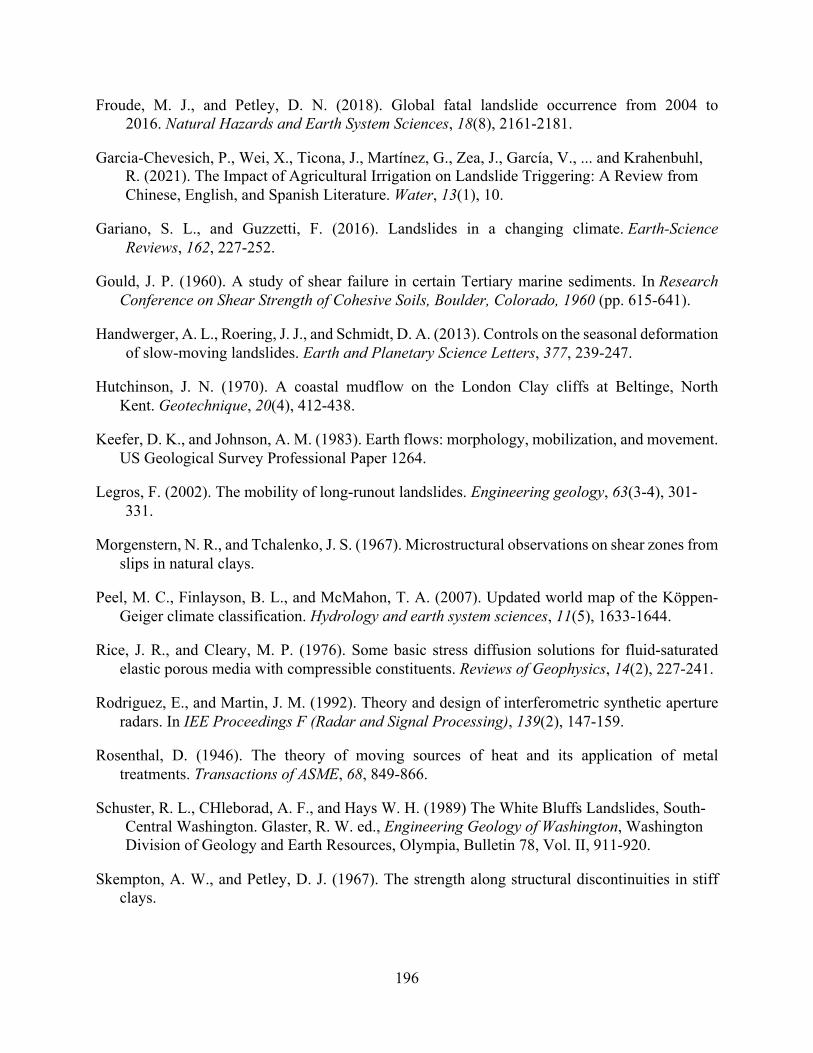
196
Froude, M. J., and Petley, D. N. (2018). Global fatal landslide occurrence from 2004 to 2016. Natural Hazards and Earth System Sciences, 18(8), 2161-2181.
Garcia-Chevesich, P., Wei, X., Ticona, J., Martínez, G., Zea, J., García, V., ... and Krahenbuhl, R. (2021). The Impact of Agricultural Irrigation on Landslide Triggering: A Review from Chinese, English, and Spanish Literature. Water, 13(1), 10.
Gariano, S. L., and Guzzetti, F. (2016). Landslides in a changing climate. Earth-Science Reviews, 162, 227-252.
Gould, J. P. (1960). A study of shear failure in certain Tertiary marine sediments. In Research Conference on Shear Strength of Cohesive Soils, Boulder, Colorado, 1960 (pp. 615-641).
Handwerger, A. L., Roering, J. J., and Schmidt, D. A. (2013). Controls on the seasonal deformation of slow-moving landslides. Earth and Planetary Science Letters, 377, 239-247.
Hutchinson, J. N. (1970). A coastal mudflow on the London Clay cliffs at Beltinge, North Kent. Geotechnique, 20(4), 412-438.
Keefer, D. K., and Johnson, A. M. (1983). Earth flows: morphology, mobilization, and movement. US Geological Survey Professional Paper 1264.
Legros, F. (2002). The mobility of long-runout landslides. Engineering geology, 63(3-4), 301-331.
Morgenstern, N. R., and Tchalenko, J. S. (1967). Microstructural observations on shear zones from slips in natural clays.
Peel, M. C., Finlayson, B. L., and McMahon, T. A. (2007). Updated world map of the Köppen-Geiger climate classification. Hydrology and earth system sciences, 11(5), 1633-1644.
Rice, J. R., and Cleary, M. P. (1976). Some basic stress diffusion solutions for fluid‐saturated elastic porous media with compressible constituents. Reviews of Geophysics, 14(2), 227-241.
Rodriguez, E., and Martin, J. M. (1992). Theory and design of interferometric synthetic aperture radars. In IEE Proceedings F (Radar and Signal Processing), 139(2), 147-159.
Rosenthal, D. (1946). The theory of moving sources of heat and its application of metal treatments. Transactions of ASME, 68, 849-866.
Schuster, R. L., CHleborad, A. F., and Hays W. H. (1989) The White Bluffs Landslides, South-Central Washington. Glaster, R. W. ed., Engineering Geology of Washington, Washington Division of Geology and Earth Resources, Olympia, Bulletin 78, Vol. II, 911-920.
Skempton, A. W., and Petley, D. J. (1967). The strength along structural discontinuities in stiff clays.
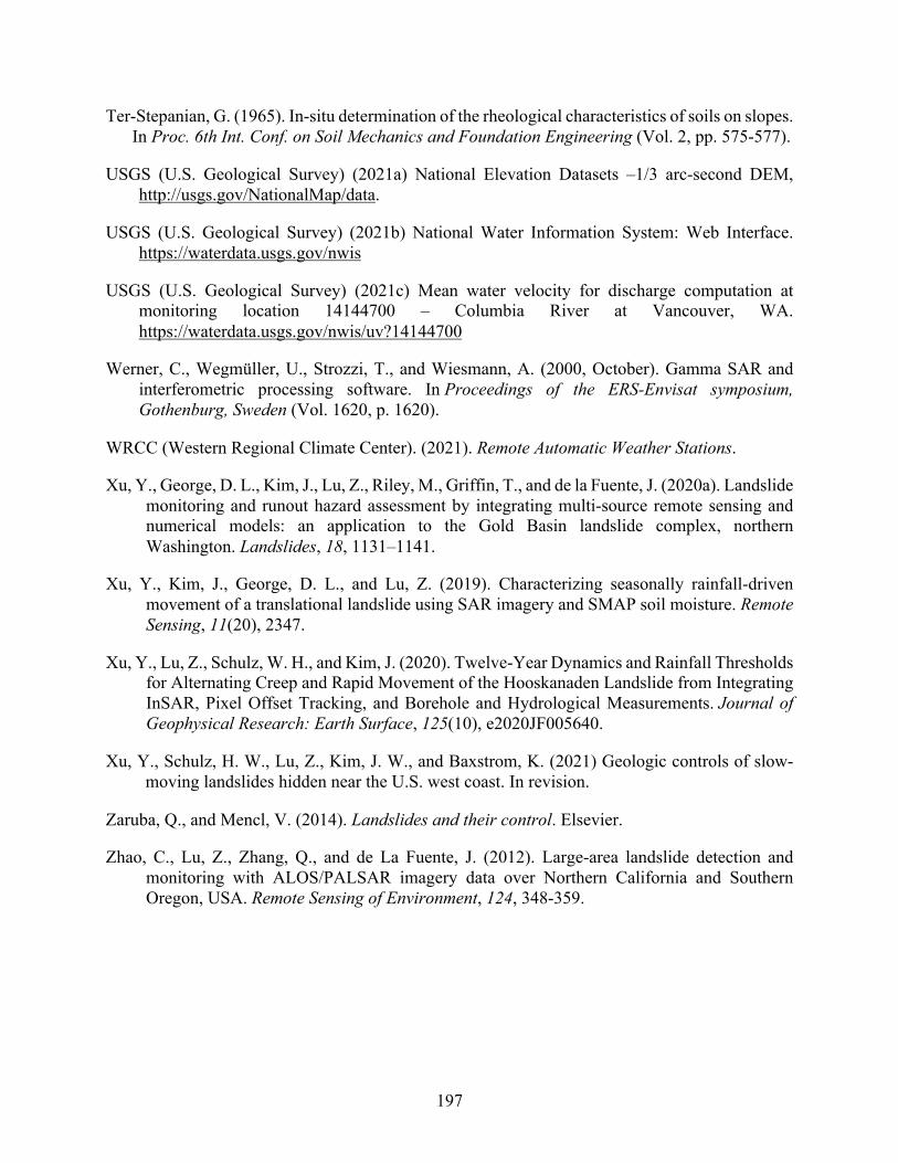
197
Ter-Stepanian, G. (1965). In-situ determination of the rheological characteristics of soils on slopes. In Proc. 6th Int. Conf. on Soil Mechanics and Foundation Engineering (Vol. 2, pp. 575-577).
USGS (U.S. Geological Survey) (2021a) National Elevation Datasets –1/3 arc-second DEM, http://usgs.gov/NationalMap/data.
USGS (U.S. Geological Survey) (2021b) National Water Information System: Web Interface. https://waterdata.usgs.gov/nwis
USGS (U.S. Geological Survey) (2021c) Mean water velocity for discharge computation at monitoring location 14144700 – Columbia River at Vancouver, WA. https://waterdata.usgs.gov/nwis/uv?14144700
Werner, C., Wegmüller, U., Strozzi, T., and Wiesmann, A. (2000, October). Gamma SAR and interferometric processing software. In Proceedings of the ERS-Envisat symposium, Gothenburg, Sweden (Vol. 1620, p. 1620).
WRCC (Western Regional Climate Center). (2021). Remote Automatic Weather Stations.
Xu, Y., George, D. L., Kim, J., Lu, Z., Riley, M., Griffin, T., and de la Fuente, J. (2020a). Landslide monitoring and runout hazard assessment by integrating multi-source remote sensing and numerical models: an application to the Gold Basin landslide complex, northern Washington. Landslides, 18, 1131–1141.
Xu, Y., Kim, J., George, D. L., and Lu, Z. (2019). Characterizing seasonally rainfall-driven movement of a translational landslide using SAR imagery and SMAP soil moisture. Remote Sensing, 11(20), 2347.
Xu, Y., Lu, Z., Schulz, W. H., and Kim, J. (2020). Twelve‐Year Dynamics and Rainfall Thresholds for Alternating Creep and Rapid Movement of the Hooskanaden Landslide from Integrating InSAR, Pixel Offset Tracking, and Borehole and Hydrological Measurements. Journal of Geophysical Research: Earth Surface, 125(10), e2020JF005640.
Xu, Y., Schulz, H. W., Lu, Z., Kim, J. W., and Baxstrom, K. (2021) Geologic controls of slow-moving landslides hidden near the U.S. west coast. In revision.
Zaruba, Q., and Mencl, V. (2014). Landslides and their control. Elsevier.
Zhao, C., Lu, Z., Zhang, Q., and de La Fuente, J. (2012). Large-area landslide detection and monitoring with ALOS/PALSAR imagery data over Northern California and Southern Oregon, USA. Remote Sensing of Environment, 124, 348-359.
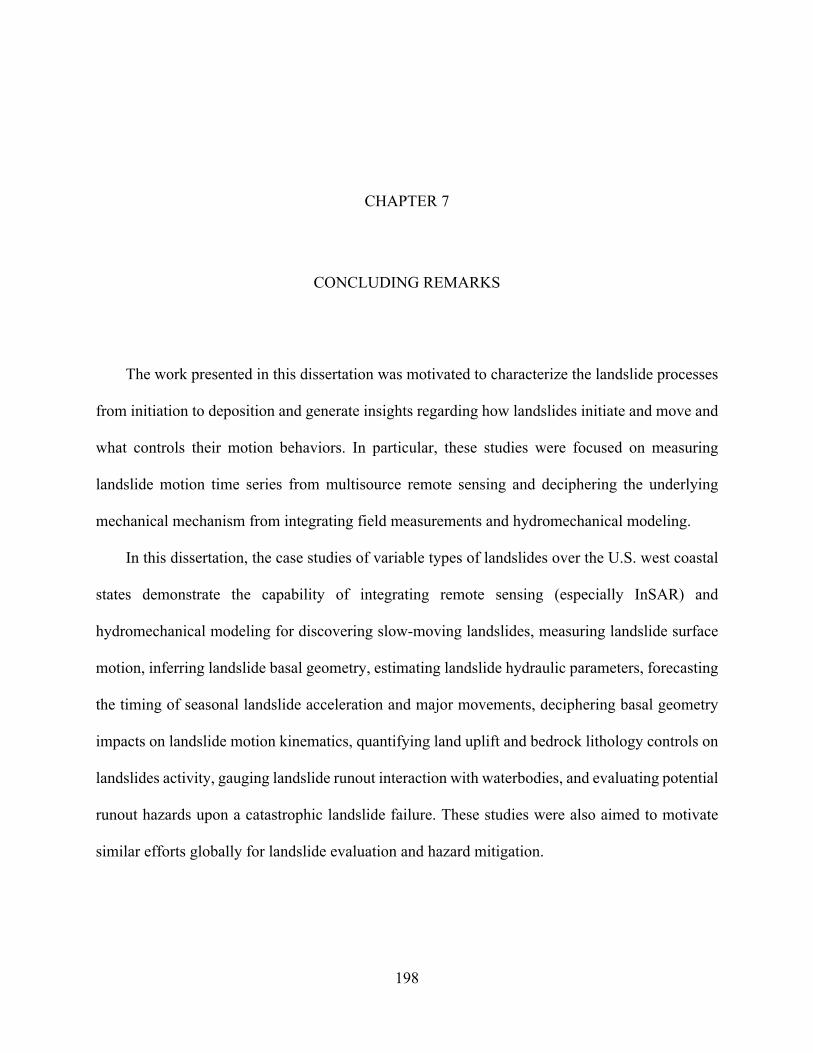
198
CHAPTER 7
CONCLUDING REMARKS
The work presented in this dissertation was motivated to characterize the landslide processes
from initiation to deposition and generate insights regarding how landslides initiate and move and
what controls their motion behaviors. In particular, these studies were focused on measuring
landslide motion time series from multisource remote sensing and deciphering the underlying
mechanical mechanism from integrating field measurements and hydromechanical modeling.
In this dissertation, the case studies of variable types of landslides over the U.S. west coastal
states demonstrate the capability of integrating remote sensing (especially InSAR) and
hydromechanical modeling for discovering slow-moving landslides, measuring landslide surface
motion, inferring landslide basal geometry, estimating landslide hydraulic parameters, forecasting
the timing of seasonal landslide acceleration and major movements, deciphering basal geometry
impacts on landslide motion kinematics, quantifying land uplift and bedrock lithology controls on
landslides activity, gauging landslide runout interaction with waterbodies, and evaluating potential
runout hazards upon a catastrophic landslide failure. These studies were also aimed to motivate
similar efforts globally for landslide evaluation and hazard mitigation.
199
7.1 Highlights
Chapter 2: This chapter was focused on a constantly (2007-2019) slow moving landslide in
Oregon. 1) Retrieving landslide motion time series from 2007 to 2011 and from 2016 to 2019 by
combining InSAR processing of both the L-band ALOS and the C-band Sentinel-1 SAR datasets.
2) Inverting pseudo-3D surface motion vectors of the landslide from both ascending and
descending InSAR measurements by assuming a dominant downslope direction (azimuth angle
only) at each SAR pixel. 3) Estimating landslide thickness from the pseudo-3D surface motions
based on volume conservation by assuming a subsurface rheology. 4) Employing an independent
limit equilibrium analysis to validate the estimated landslide thickness from surface motion
vectors. 5) Integrating landslide motion time series and satellite-sensed shallow soil moisture to
obtain time lags between the onset of wet season and the seasonal acceleration of landslide
movement. 6) Incorporating rainfall infiltration and pore-pressure diffusion models to estimate
hydraulic conductivity and diffusivity.
Chapter 3: This chapter was focused on a coastal landslide in Oregon with alternating slow
and rapid motions. 1) Combining sub-pixel offset tracking measurements of both the Sentinel-1
SAR images and the Sentinel-2 optical images to reconstruct 3D surface motion vectors of a 2019
major landslide movement. 2) Integrating InSAR processing of the ALOS and Sentinel-1 imagery
and sub-pixel offset tracking of LiDAR DEM gradients to retrieve a 12-year motion time series of
the landslide. 3) Proposing a novel three-factor threshold that relies on water-year and previous
3-day and daily precipitation to temporally forecast major landslide movements. 4) Revealing that
coastal erosion has been accelerating the landslide motion from 2007 to 2019 by eroding the
landslide toe.
200
Chapter 4: This chapter was focused on a potentially catastrophic landslide near a popular
campground in northern Washington. 1) Integrating multisource remote sensing datasets (LiDAR
DEM, SAR, optical images) and techniques (DEM differencing, sub-pixel offset tracking, radar
interferometry) to monitor recent landslide activity. 2) Combining remote sensing measurements
and 3D limit equilibrium analyses to constrain the potential landslide volume. 3) Incorporating the
D-claw runout model to evaluate potential landslide runout hazards. 4) Simulating a naturally
flowing river at the landslide tor and evaluating the river’s impacts on landslide mobility and the
corresponding runout hazards.
Chapter 5: This chapter was focused on discovering slow-moving landslides over the entire
U.S. west coastal states and deciphering their geologic controls. 1) Discovering 601 active, large
landslides that were previously unknown in Washington, Oregon, and California using SAR
interferometry from 2007 to 2011 and from 2015 to 2019. 2) Revealing that bedrock lithology
controls size and spatial density of the identified active landslides. 3) Discovering that land uplift
in a geologic scale might contribute to landslide occurrence and activity.
Chapter 6: This chapter was focused on landslides in a Washington desert induced by
agricultural irrigation. 1) Uncovering 13 active, slow-moving landslide complex and 12
catastrophic landslides along a Washington dessert valley from satellite radar and optical images.
2) Verifying that agricultural irrigation induces landslides by reducing soil shearing strength and
elevating groundwater level. 3) Discovering that landslides with toes in the Columbia River were
strongly impacted by water level of the river, whereas the landslides far away from the river
primarily depended on irrigation water seepage and the induced groundwater changes. 4)
Revealing that basal topography fundamentally impacts motion kinematics of slow landslides
through forced water circulation, and affects catastrophic landslides through kinetic energy gain.
201
7.1 Future Work
Based on the knowledge and experience gained from the completed landslide case studies,
my future research work will be focused on the following five aspects:
1) Discovering active landslides over the entire conterminous United States using
InSAR. Active landslides consistently damage infrastructures such as highways and buildings and
cause constant repair and maintenance costs to state and federal agencies and homeowners.
Moreover, active landslides indicate a force imbalance of the hillslopes and could evolve into a
future catastrophic disaster under disturbances from such as earthquake shaking, intense rainfall,
and anthropogenic activities. Locating these unstable slopes is the first step and a critical step to
reduce their future hazards. I will use InSAR processing of primarily the free L-band ALOS SAR
images to identify active landslides over the conterminous United States.
2) Using P-band SAR for uncovering landslides hidden under dense forests. Our multiple
case studies of mapping landslides near the U.S. west coast show that the data acquired by SAR
sensors with longer wavelength perform better in discovering landslides in densely vegetated
regions. For example, the L-band (~ 23.6 cm wavelength) ALOS and ALOS-2 images were able
to produce SAR interferograms with lower background noises than the C-band (5.6 cm
wavelength) Sentinel-1 images, because the longer-wavelength SAR sensor possesses better
vegetation penetration capability. However, the spaceborne L-band SAR data still suffer from
considerable coherence loss in very densely forested regions near the U.S. west coast, which could
potentially render some landslides undetectable. To address this problem, we are collaborating
with National Aeronautics and Space Administration (NASA) to fly airborne P-band SAR (70 cm
wavelength) over multiple selected densely vegetated areas in Washington, Oregon, and California
202
to investigate if P-band SAR could be an effective solution for discovering landslides hidden under
the dense forest canopy.
3) Assessing impacts of the interaction between debris flow and waterbodies. Our case
study at the Gold Basin landslide complex show that the interaction between landslide-initiated
debris flow and a flowing river could affect landslide mobility and hence the runout hazards. Such
interactions may have variable implications depending on the geological, hydrological, and
topographical settings of a specific landslide. For example, a giant landslide failing into a lake
could generate a tsunami and propagate the hazard by tens of kilometers to the other side of the
lake bank. A failed landslide body interacting with a reservoir could cause a dam breach and lead
to disastrous flooding down the stream. Consequently, it is critical to evaluate not only the
landslide failure itself but also the potential secondary hazards from interacting with waterbodies.
I will continue to work with Dr. David George to understand and numerically simulate how the
interactions between landslide-initiated debris flow and variable waterbodies could affect landslide
post-failure hazards.
4) Deciphering the length of the precursory motion period for variable landslides. My
recent InSAR studies of multiple catastrophic landslides show that some landslides underwent
months-long continuous precursory slow motion preceding the catastrophic failure (e.g., the 2013
Cape Meares landslide in Oregon, the 2020 Elliot Creek landslide in Canada, and the 2021 Chunchi
landslide in Ecuador), whereas some experienced no precursory motion within 12 days ahead of
the failure (e.g., the 2019 Brumadinho dam failure in Brazil). Deciphering why variable landslides
have different time length of precursory motion is critical for establishing effective landslide early
warning systems. I will retrieve precursory motion time series of multiple catastrophic landslides
203
occurred after 2016 around the globe, and utilize mechanical models to understand what potential
factors determine the precursory time length of different catastrophic landslides.
5) Developing a pipeline for landslide early warning from InSAR derived precursory 3D
motions. For catastrophic landslide with continuous precursory motions for at least 24 days
preceding the final failure, I will develop a pipeline to evaluate their post-failure runout hazards
from InSAR derived 3D precursory motion. Note that I have discovered at least three catastrophic
landslides with months-long precursory motions (e.g., the 2013 Cape Meares landslide in Oregon,
the 2020 Elliot Creek landslide in Canada, and the 2021 Chunchi landslide in Ecuador). In
particular, I will use both ascending and descending InSAR to derive 3D surface motion vectors
of a landslide, and then estimate the active landslide volume from precursory surface motions
using thickness inversion models, and then input the inverted landslide basal surface into the D-
claw runout model to estimate its potential runout hazards. Moreover, another line of this work
will be focused on temporally forecasting landslide failures based on their precursory motion time
series. Mechanical modeling will be incorporated to interpret and predict the failure time.