UPTEC Q 18014

Examensarbete 30 hpJuni 2018

Characterization of a refractory cement and sensor development for temperature measurements in molten steel

Pierre Sandin

Teknisk- naturvetenskaplig fakultet UTH-enheten Besöksadress: Ångströmlaboratoriet Lägerhyddsvägen 1 Hus 4, Plan 0 Postadress: Box 536 751 21 Uppsala Telefon: 018 – 471 30 03 Telefax: 018 – 471 30 00 Hemsida: http://www.teknat.uu.se/student

Abstract

Characterization of a refractory cement and sensordevelopment for temperature measurements inmolten steelPierre Sandin

In steel manufacturing, temperature control is a critical parameter, as it is extremely important for the steel quality. In general, disposable sensors are regularly immersed in the melt for temperature measurements. There are commercially available sensors for continuous temperature measurements.

In this study, a refractory cement is used for encapsulation and carrier of a resistive temperature detector, for continuous temperature measurements in molten steel. This cement is normally used for manufacturing of steel melt crucibles. The work in this study is mostly experimental and consist of characterization of the cement and development of the sensor. The characterization includes the mechanical properties, the thermal shock resistance, the steel melt resistance and obtainable surface roughness, for different powder fractions, water-to-cement ratio, firings and mixing method. Process developments were also done for the manufacturing of the sensor element and its carrier system.

The end goal for continuous temperature measurement in molten steel for more than 60 minutes was not reached. However, functional sensors were developed where temperatures up to 1000 °C were measured during calibrations, and the cement was well characterized.

This work has been carried out within the Strategic innovation program "Smartare Elektroniksystem", a joint investment of Vinnova, Formas and Energimyndigheten.

ISSN: 1401-5773, UPTEC Q 18014Examinator: Åsa Kassman RudolphiÄmnesgranskare: Klas HjortHandledare: Greger Thornell och Lena Klintberg

Karakterisering av ett eldfast cement och framtagningav en sensor för temperaturmätningar i smält stål

Pierre Sandin

Att ha koll på temperaturen vid ståltillverkning är mycket kritiskt då det påverkar stålkvaliteten.Ett senare steg vid tillverkning av rostfritt stål tillverkning är avkolning. Här hälls smältan med enkolhalt på cirka 1 vikt% kol och en temperatur på 1600 C ner i en AOD–konverter (argon–syre–avkolning, fr. eng. Argon–Oxygen–Decarburization). I AOD–konvertern kan temperaturen gå upptill 1800 C när ämnen med hög syreaffinitet oxideras, en raffinering av stålet. Normalt så mäts tem-peraturen med engångssensorer som förs ner i smältan då och då. Kontinuerlig temperaturmätningär eftertraktat då det ger en bättre bild av hela förloppet. Det finns idag sensorer som kan användasi kontinuerlig drift, vare sig det är sensorer som är i direkt kontakt med smältan eller de som inteär det. De sensorer som är i direkt kontakt med smältan behöver vara skyddade av material sombåde tål hög temperatur och den kemiskt aggresiva miljön. I detta arbete används ett eldfast cementmed en maximal användningstemperatur på 1800 C, som skyddande hölje och hållare till en utveck-lad resistiv temperaturgivare. Det eldfasta cementet används till deglar för smält stål. Arbetet ärmestadels experimentellt, där karakterisering av cementet görs i form av hållfasthet, motstånd motstålsmälta, mikrostruktur, ytfinhet och gjutbarhet för olika recept. Dessutom igår framtagning avsensorelementet och dess interaktion med cementet.

Olika pulverfraktioner, vattenmängder och eldningar testades för cementet. Här analyserades hållfas-theten före och efter termisk chock i form av trepunkts balkböjning på gjutna balkar. Vissa av receptentestades i olika stålsmältor med temperaturer över 1500 C, i form av stavar. Sensorn består av deteldfasta cementet, en tunn platina struktur och trådar av platina. Metallstrukturen skapades med enmetod kallad screentryckning, vilket är en fungerande metod för högtemperatur–sambrändakeramer.Denna process utvecklades för att fungera med cementsystemet. De olika stegen för framtagningav olika gjutprocesser var sensorkroppen och dess hållarsystem, ingjutningar av kontakteringstrådar,samt de olika former som används vid materialkaratäriseringen.

Böjhållfastheten och böjmodulen var bäst för cementet med ett pulver bestående av de minsta partik-larna. Alla recept klarade termochock–testerna, där de icke–eldade balkarna därefter fick en förhöjdhållfasthet. Bränningen gav i de flesta fall cementet en högre böjhållfasthet och böjmodul.

Ytfinheten var som bäst för cementet då det göts i en Petri–skål. Där uppnådes en ytfinhet som bästpå hundradels mikrometer i Ra–värde. Från göt i PDMS formar var Ra–värdet i tiondels mikrometer.

Ingen av teststavarna överlevde i mer än 5 minuter i stålsmältorna. Endast en var hel efter att ha bliviturtagen ur smältan efter 5 minuter. Tvärsnitt analyserades där det observerades att stål–material hadetagit sig in i staven.

Av de framtagna sensorerna fungerade initialt ∼33 % och efter reparationer ∼66 %. Två av sensorernakalibrerades, vid uppmätt temperatur upp till 1000 C. Dessa testades sedan i stålsmälta. Sensorernasattes i två olika hållarlansar. En Sialon– och en cementlans. Sialon–lansen höll ca 16 minuter ochcementlansen höll kortare tid. Uppmätt signal kunde bara fås från Sialon–lansen, då en kontakter-ingstråd gick av i cementlansen vid nedföring i smältan.

Arbetet har utförts inom Strategiska innovationsprogrammet "Smartare Elektroniksystem" en gemen-sam satsning av Vinnova, Formas och Energimyndigheten.

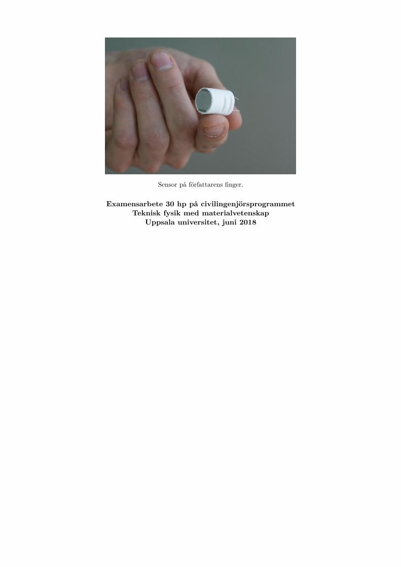
Sensor på författarens finger.

Examensarbete 30 hp på civilingenjörsprogrammetTeknisk fysik med materialvetenskap

Uppsala universitet, juni 2018

Acknowledgments

Many thanks to Greger and Lena for being such supportive and helpful supervisors. Thank youGreger for guiding me through the jungle of interesting experiments and for all the shared ideas withthe process developments. Thank you Lena for all the laboratory work you have helped me with andthe positive spirit you brought when I was in despair. I would also like to thank all of the microsystem technology department, mostly Erika, Peter and Ragnar for all the interesting discussions andhelp, whether it was experimental work or just a ride to the hardware store. Many thanks to Andersfrom the tribology group for the SEM images you helped me with. This project was introduced tome by Klas which I’m grateful for. Finally, I would like to extend my gratitude to Sandvik MaterialTechnologies, especially Fredrik for involving me in an very interesting and real project.

Contents

1 Introduction 1

2 Background 22.1 Steel refinement and temperature sensing . . . . . . . . . . . . . . . . . . . . . . . . . 22.2 Cement and refractory castables . . . . . . . . . . . . . . . . . . . . . . . . . . . . . . 22.3 Screen printing . . . . . . . . . . . . . . . . . . . . . . . . . . . . . . . . . . . . . . . . 3

3 Theory 43.1 Solid mechanics . . . . . . . . . . . . . . . . . . . . . . . . . . . . . . . . . . . . . . . . 43.2 Thermal sensors . . . . . . . . . . . . . . . . . . . . . . . . . . . . . . . . . . . . . . . 5

4 Materials and methods 64.1 Moulds . . . . . . . . . . . . . . . . . . . . . . . . . . . . . . . . . . . . . . . . . . . . 74.2 Casting . . . . . . . . . . . . . . . . . . . . . . . . . . . . . . . . . . . . . . . . . . . . 84.3 Metallization process development . . . . . . . . . . . . . . . . . . . . . . . . . . . . . 10

4.3.1 Thick film characteristics . . . . . . . . . . . . . . . . . . . . . . . . . . . . . . 114.4 Material characterization . . . . . . . . . . . . . . . . . . . . . . . . . . . . . . . . . . 12

4.4.1 Thermal shock . . . . . . . . . . . . . . . . . . . . . . . . . . . . . . . . . . . . 124.4.2 Three–point beam bending . . . . . . . . . . . . . . . . . . . . . . . . . . . . . 124.4.3 Corrosion test . . . . . . . . . . . . . . . . . . . . . . . . . . . . . . . . . . . . . 134.4.4 Surface analysis . . . . . . . . . . . . . . . . . . . . . . . . . . . . . . . . . . . . 13

4.5 Sensor design . . . . . . . . . . . . . . . . . . . . . . . . . . . . . . . . . . . . . . . . . 144.5.1 Sensor body . . . . . . . . . . . . . . . . . . . . . . . . . . . . . . . . . . . . . . 144.5.2 Sensor element . . . . . . . . . . . . . . . . . . . . . . . . . . . . . . . . . . . . 15

4.6 Lance systems . . . . . . . . . . . . . . . . . . . . . . . . . . . . . . . . . . . . . . . . . 164.6.1 Sialon lance . . . . . . . . . . . . . . . . . . . . . . . . . . . . . . . . . . . . . . 164.6.2 Cement lance . . . . . . . . . . . . . . . . . . . . . . . . . . . . . . . . . . . . . 18

4.7 Sensor calibration . . . . . . . . . . . . . . . . . . . . . . . . . . . . . . . . . . . . . . . 194.8 Field testing of sensors . . . . . . . . . . . . . . . . . . . . . . . . . . . . . . . . . . . . 20

5 Results 215.1 Evaluation of metallization process . . . . . . . . . . . . . . . . . . . . . . . . . . . . . 215.2 Material properties . . . . . . . . . . . . . . . . . . . . . . . . . . . . . . . . . . . . . . 22

5.2.1 Bending strength . . . . . . . . . . . . . . . . . . . . . . . . . . . . . . . . . . . 225.2.2 Corrosion test of rods . . . . . . . . . . . . . . . . . . . . . . . . . . . . . . . . 25

5.2.2.1 First test rods . . . . . . . . . . . . . . . . . . . . . . . . . . . . . . . 255.2.2.2 Second test rods . . . . . . . . . . . . . . . . . . . . . . . . . . . . . . 285.2.2.3 Third test rods . . . . . . . . . . . . . . . . . . . . . . . . . . . . . . . 28

5.2.3 Surface roughness . . . . . . . . . . . . . . . . . . . . . . . . . . . . . . . . . . 295.3 Sensor element yield . . . . . . . . . . . . . . . . . . . . . . . . . . . . . . . . . . . . . 305.4 Temperature measurements . . . . . . . . . . . . . . . . . . . . . . . . . . . . . . . . . 31

5.4.1 Sensor calibration . . . . . . . . . . . . . . . . . . . . . . . . . . . . . . . . . . 315.4.2 Field testing . . . . . . . . . . . . . . . . . . . . . . . . . . . . . . . . . . . . . 32

6 Discussion 346.1 Processing . . . . . . . . . . . . . . . . . . . . . . . . . . . . . . . . . . . . . . . . . . . 346.2 The material properties . . . . . . . . . . . . . . . . . . . . . . . . . . . . . . . . . . . 34

6.2.1 Mechanical and thermal shock properties . . . . . . . . . . . . . . . . . . . . . 346.2.2 Cement and melt interaction . . . . . . . . . . . . . . . . . . . . . . . . . . . . 35

6.3 Metallization and sensor yield . . . . . . . . . . . . . . . . . . . . . . . . . . . . . . . . 356.4 Sensor functionality . . . . . . . . . . . . . . . . . . . . . . . . . . . . . . . . . . . . . 366.5 Final discussion . . . . . . . . . . . . . . . . . . . . . . . . . . . . . . . . . . . . . . . . 36

7 Future work 37

8 Conclusions 37

List of Figures1 Screen and paste example . . . . . . . . . . . . . . . . . . . . . . . . . . . . . . . . . . 32 Force deflection cruve . . . . . . . . . . . . . . . . . . . . . . . . . . . . . . . . . . . . 43 Casting moulds . . . . . . . . . . . . . . . . . . . . . . . . . . . . . . . . . . . . . . . . 74 Firing profiles . . . . . . . . . . . . . . . . . . . . . . . . . . . . . . . . . . . . . . . . . 95 Test pattern for screen printing . . . . . . . . . . . . . . . . . . . . . . . . . . . . . . . 106 Firing profile at 1400 C of the Pt paste . . . . . . . . . . . . . . . . . . . . . . . . . . 107 Probe station . . . . . . . . . . . . . . . . . . . . . . . . . . . . . . . . . . . . . . . . . 118 Bending setup . . . . . . . . . . . . . . . . . . . . . . . . . . . . . . . . . . . . . . . . . 129 Dipping test . . . . . . . . . . . . . . . . . . . . . . . . . . . . . . . . . . . . . . . . . . 1310 Sensor body casting . . . . . . . . . . . . . . . . . . . . . . . . . . . . . . . . . . . . . 1411 Sensor element structure . . . . . . . . . . . . . . . . . . . . . . . . . . . . . . . . . . . 1512 Sensor body and element assembly . . . . . . . . . . . . . . . . . . . . . . . . . . . . . 1513 Point welding . . . . . . . . . . . . . . . . . . . . . . . . . . . . . . . . . . . . . . . . . 1614 Technical drawing of the sialon lance . . . . . . . . . . . . . . . . . . . . . . . . . . . . 1715 Sensor insertion in the lance . . . . . . . . . . . . . . . . . . . . . . . . . . . . . . . . . 1716 Casting of the cement lance . . . . . . . . . . . . . . . . . . . . . . . . . . . . . . . . . 1817 Sensor calibration set–up . . . . . . . . . . . . . . . . . . . . . . . . . . . . . . . . . . 1918 First sensor calibration . . . . . . . . . . . . . . . . . . . . . . . . . . . . . . . . . . . . 2019 Lances in field test . . . . . . . . . . . . . . . . . . . . . . . . . . . . . . . . . . . . . . 2020 Metallization evaluation . . . . . . . . . . . . . . . . . . . . . . . . . . . . . . . . . . . 2121 Flexural strength before and after thermal shock . . . . . . . . . . . . . . . . . . . . . 2222 Flexural modulus before and after thermal shock . . . . . . . . . . . . . . . . . . . . . 2323 EDS mapping of test beam C1 . . . . . . . . . . . . . . . . . . . . . . . . . . . . . . . 2324 EDS mapping of test beam A1 . . . . . . . . . . . . . . . . . . . . . . . . . . . . . . . 2325 Joint beam strenght . . . . . . . . . . . . . . . . . . . . . . . . . . . . . . . . . . . . . 2426 C1F4 rod cross section . . . . . . . . . . . . . . . . . . . . . . . . . . . . . . . . . . . . 2527 First EDS line scan . . . . . . . . . . . . . . . . . . . . . . . . . . . . . . . . . . . . . . 2628 Second EDS line scan . . . . . . . . . . . . . . . . . . . . . . . . . . . . . . . . . . . . 2729 Corrosion and cross section of A1 rods . . . . . . . . . . . . . . . . . . . . . . . . . . . 2830 Surface profile over connection wires . . . . . . . . . . . . . . . . . . . . . . . . . . . . 2931 Surface compairson . . . . . . . . . . . . . . . . . . . . . . . . . . . . . . . . . . . . . . 3032 Sensor repair example . . . . . . . . . . . . . . . . . . . . . . . . . . . . . . . . . . . . 3033 Heating and resistance cycle in sensor calibration . . . . . . . . . . . . . . . . . . . . . 3134 Resistance stabilization between calibration iterations . . . . . . . . . . . . . . . . . . 3135 Sensor calibration fit . . . . . . . . . . . . . . . . . . . . . . . . . . . . . . . . . . . . . 3236 Wire fracture in the cement lance . . . . . . . . . . . . . . . . . . . . . . . . . . . . . . 3237 Sampled data from the Sialon lance . . . . . . . . . . . . . . . . . . . . . . . . . . . . . 3338 Cross section of cement lance . . . . . . . . . . . . . . . . . . . . . . . . . . . . . . . . 33

List of Tables1 Part of MiMix technical data sheet . . . . . . . . . . . . . . . . . . . . . . . . . . . . . 82 Castings for material characterization . . . . . . . . . . . . . . . . . . . . . . . . . . . 93 Electrical characteristics and thickness of the prints . . . . . . . . . . . . . . . . . . . . 214 Thermo mechanical porperties of beams . . . . . . . . . . . . . . . . . . . . . . . . . . 225 Joint beams strength . . . . . . . . . . . . . . . . . . . . . . . . . . . . . . . . . . . . . 246 Surface rougness results . . . . . . . . . . . . . . . . . . . . . . . . . . . . . . . . . . . 29

Nomenclature

AbbreviationsAOD Argon–Oxygen–DecarburizationCAC Calcium aluminate cementDAQ Data acquisitionEDS Energy–dispersive X–ray spectroscopyHTCC High temperature co–fired ceramicLCC Low cement castablePDMS PolydimethylsiloxanePVC Polyvinyl chlorideRTD Resistive temperature detectorSEM Scanning electron microscopeTs1 Thermal shock 1Ts2 Thermal shock 2ULCC Ultra low cement castableUV Ultraviolet

1 IntroductionOne of the later process steps in stainless steel manufacturing is decarburization. Here the 1600 Cmelt is poured into a converter. A common converter is the AOD (Argon–Oxygen–Decarburization)converter. Here the steel melt has initially about 1 wt% of C. By blowing Ar and O into the melt,elements with high oxygen affinity, such as C, Si, Cr and Mn, oxidise. The temperature of the meltrises since the oxidation processes are exothermical. Pb, Zn and Bi evaporate in the process, relievingthe melt of unwanted trace elements. After the decarburization, the slag is reduced with the additionof ferrosilicon and lime under mixing with Ar, reducing the CrO and MgO. Refining of the melt isdone after the reduction process. This is also done under mixing with argon and addition of reductionelements, e.g., Al [1].

The steel melt spends about 60 to 90 minutes in the converter. During this time, it would be preferableto be able to monitor parameters such as temperature, flow and chemical composition continuously.In this project, a refractory cement is investigated for use as a carrier and encapsulation for a metallictemperature sensing device, for immersion in molten steel. The refractory cement is the same materialas is used in the manufacturing of steel melt crucibles. The project is a cooperation between UppsalaUniversity and Sandvik Material Technology, where the goal is to provide new ideas and informationthat could benefit the company in the production.

The device is first of all intended to be a temperature sensor, but as the manufacturing gives muchroom for design changes, there are possibilities to measure also, e.g., flow. To prepare for this, therefractory cement has to be studied both on its own and in combination with the sensor device. Aprocessing method for making the sensor is also needed.

The studies in this project are mostly experimental, and consist of mechanical, thermomechanical,chemical and casting characterization of a refractory cement as well as the investigation of the in-teraction between the castable and sensor. The end goal of the project is to perform a continuoustemperature measurement in a melt for over 60 minutes.

1

2 Background

2.1 Steel refinement and temperature sensing

Sandvik Materials Technology is a world–leading company that develops advanced stainless steel andspecial alloys for applications in demanding environments. Development of these materials requiresgreat process control. At the test facility, where new stainless steel and special alloys are developed,new techniques of measuring temperature, element concentration and flow characteristics are needed.In this project, the focus has been on measuring the temperature of the metal melt for long timeperiods. The vision is that a similar system later is to be used in the AOD converter.

In general, disposable thermocouples are regularly immersed in the melt to measure the temperature,as the molten steel temperature is extremely important for the steel quality [2]. Commercial technolo-gies for measurement of temperature, oxygen and carbon content are provided by many companies.For example, the company Mekinor metall AB provides combi–sensors that can measure the oxygenactivity, carbon concentration, temperature and extract a sample from the melt, for use in LD (Linz—Donawitz) converters a.k.a. basic oxygen converters. The accuracy of these probes are in the order of±0.01 % C, in the ranges of 0.2 – 1 % C within a time of 3 to 6 seconds to measure the temperature[3]. The temperature and O content range and accuracy are not specified. Another company thatprovides disposable sensors is Karrich industries inc. Available products are thermocouples, oxygenprobes, immersion samplers and carbon/temperature sensors. Their oxygen probe are designed tomeasure oxygen levels from 1 ppm to 2599 ppm [4]. The company Ferrotron can provide immersionprobes that can measure temperatures >1520 C and also have an immersion sensor, FOXTM (Fer-rotron Oxygen activity measurement probe), which can measure temperatures up to 1800 C. Theseprobes have a response time of 1–3 seconds [5, 6].

Continuous temperature measurement in molten steel can be provided by the company HeraeusElectro–Nite with their CastempR© sensor. This sensor probe consists of a type B thermocouplehoused in a robust refractory sheet, resistant to thermal shock, and gives a fast temperature response.Displayed usage temperature is at 1550 C. [7] Non–contact temperature measuring from 0 to 3000C can be provided by the company Keller ITS, as pyrometers [8].

Recent studies for continuous temperature measurement at these high melt temperatures are mostlyfocused on the use of black body radiation, [9, 10], as thermocouple prices are high, [11]. Electricalsystems are though interesting at lower temperature as they have the potential to be constructed forsimultaneous measurements of different physical parameters, e.g., temperature and flow, [12].

2.2 Cement and refractory castables

Joseph Aspdin patented a cement in 1824 and called it Portland cement, where the name comes froma stone called Portland stone. The patent was entitled "An Improvement in the Mode of Producing anArtificial Stone" [13]. Generally, cement is a binder substance and can be characterised as hydraulicor non–hydraulic depending on if addition of water is needed for curing. Non–hydraulic cements needcarbon dioxide for carbonation, where water is produced. Hydraulic cements cure with the additionof water, called hydration. The mass of added water to cement mass is called the water–to–cement(w/c) ratio. The w/c ratio is typically ≥0.38 wt% to achieve full hydration for construction cement.Adding too much water can cause incomplete hydration, leaving water–filled capillary pores behind.The strength of Portland cement comes mostly from alite (tricalcium silicate, Ca3SiO5) and belite (di-calcium silicate, Ca2SiO4) [14]. When mixing the cement and water, air bubbles are usually trapped.These are usually removed by vibration. In macro scale casting of constructional cement, trapped airis removed by immersing a hand–held vibrating rod.

2

In 1908, Jules Bied patented cement containing a mixture of limestone and aluminous substances. Itbecame known as "ciment fondu", which roughly translates to fused cement. It was developed to with-stand chemical attacks by sulphates. Mixed with appropriate refractory aggregates, calcium aluminatecements can be made to withstand temperatures up to 2000 C. They are not only heat resistance butalso very resistant to thermal shock.[14] The basic difference between Portland cement and calciumaluminate cements (CACs) is the active phase leading to curing. As Portland cement contains CaOand SiO2 in the forms of alite and belite, the addition of water creates the hydrates, calcium silicatehydrate and calcium hydroxide. As for CACs, there is little to no SiO2 content. The main oxides areCaO and Al2O3, which with the addition of water create calcium aluminate hydrates.[15] Refractorycastables are dry granulated materials which require water addition for curing [16], i.e., hydraulic.Refracory castables can be categorised by their cement content, more exactly their CaO and SiO2content, for example ultra low cement castables (ULCC) and low cement castable (LCC) [17, 18].Compared to Portland cement, the w/c ratio is typically much lower. The refractory castable used inthis study, MiMix CA 97 GK, could be categorised as an ULCC. It is based on the alumina mineralCorundum. For simplicity, this refractory castable will be refereed to simply as cement from now on.

For continuous contact measurements, the active sensor device has to be protected by a refractory andchemically inert material. The refractory cement, Mimix Ca 97 GK, will be evaluated in this studyas the encapsulation to a resistive temperature device for measurements in molten steel.

2.3 Screen printing

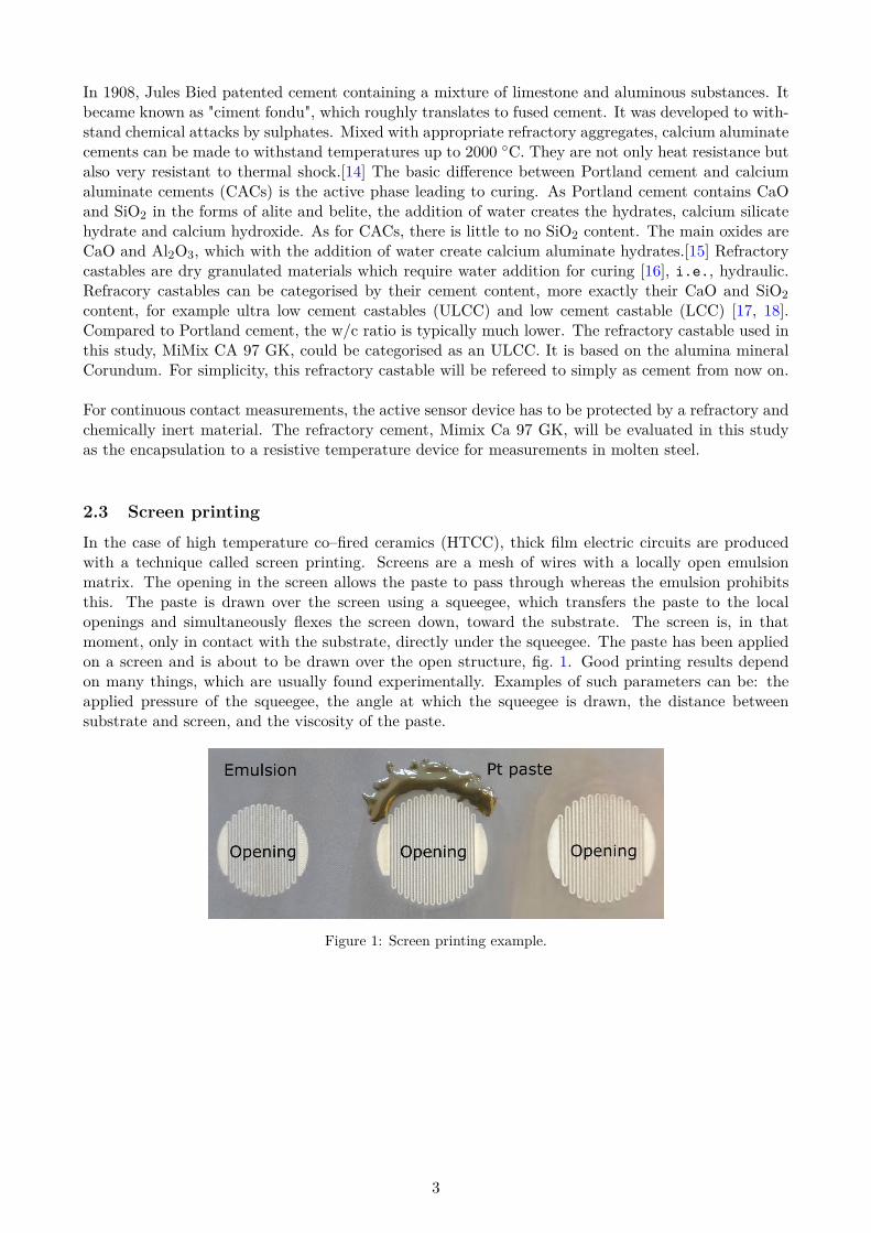
In the case of high temperature co–fired ceramics (HTCC), thick film electric circuits are producedwith a technique called screen printing. Screens are a mesh of wires with a locally open emulsionmatrix. The opening in the screen allows the paste to pass through whereas the emulsion prohibitsthis. The paste is drawn over the screen using a squeegee, which transfers the paste to the localopenings and simultaneously flexes the screen down, toward the substrate. The screen is, in thatmoment, only in contact with the substrate, directly under the squeegee. The paste has been appliedon a screen and is about to be drawn over the open structure, fig. 1. Good printing results dependon many things, which are usually found experimentally. Examples of such parameters can be: theapplied pressure of the squeegee, the angle at which the squeegee is drawn, the distance betweensubstrate and screen, and the viscosity of the paste.

Figure 1: Screen printing example.

3

3 Theory

3.1 Solid mechanics

To characterize the mechanical strength of ceramics, different tests can be done. A common propertyis cold compression strength (CCS), where a cube of specified size is crushed between two pistons.Another common mechanical strength property is flexural strength, which is a property obtained fromfour–point or three–point beam bending. Flexural strength, σf , is the maximum stress just beforethe material fractures. In three–point bending, the beam rests on a support in each end, and a forceis applied in the middle. These test are performed with help of the American Society for TestingMaterials (ASTM) standard [19]. The ASTM standard C1161–13 handles testing methods for flexuralstrength of advanced ceramics at ambient temperatures. The obtained properties are flexural strengthand flexural modulus [20]. The flexural strength (σf ), depends on the applied force, the beams crosssection dimensions and the distance between the supports as,

σf = 3FmaxL

2wt2 , (1)

where Fmax is the maximum force before the material fractures, L is the length of between supportsand w is the width and t is the thickness of the beam. The 2nd moment of inertia of a rectangularcross section is

I = wt3

12 . (2)

The flexural modulus (Ef ), depends on the 2nd moment on inertia, the distance between the supportsand the slope of most linear part of the force vs. deflection curve as,

Ef = L3m

48I , (3)

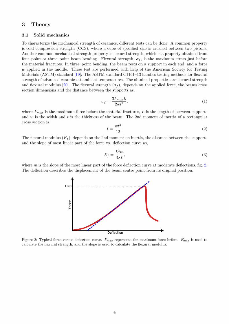
where m is the slope of the most linear part of the force deflection curve at moderate deflections, fig. 2.The deflection describes the displacement of the beam centre point from its original position.

Figure 2: Typical force versus deflection curve. Fmax represents the maximum force before. Fmax is used tocalculate the flexural strength, and the slope is used to calculate the flexural modulus.

4

3.2 Thermal sensors

Thermocouples are well known temperature sensors consisting of two different fused metal wires, wherethe Seebeck effect correlates the electrical potential to temperature according to

V = β∆T, (4)

where V is the generated voltage, β is the Seebeck coefficient and ∆T it the temperature differencebetween the hot and cold junctions [21]. The two different metal wires are fused together at their endsand may consist of W and Re for measurements at high temperatures [22]. The joint which is placedat the measurement point is called the hot junction. The other end, the cold junction is kept at aconstant temperature, usually 0 C. The temperature difference will induce a proportional electricalpotential in the wires.

Thermistors are a type of temperature sensors where the resistivity of the material changes withtemperature. Thermistors are usually ceramics or polymers and are not to be confused with resistancetemperature detectors (RTD), which are metal based. Thermistors are semiconductors, where theresistance–to–temperature dependence can be described by

RT = R0 · exp[1 −B

( 1T

− 1T0

)], (5)

where R0 is the resistance at the reference temperature T0, and B is a constant [22]. Thermistors caneither have a positive or negative temperature coefficient, depending on the semiconductor materials,meaning a decrease or increase of resistivity with increasing temperature, respectively. Thermistorsare usually good choices when accuracy is not critical [22].

RTDs are a good choice for large temperature ranges and are usually made with platinum due toits almost linear dependence. RTD sensors can also be produced with accuracies of µK [22]. Thetemperature dependence follows

ρ(T ) = ρ0 · [1 + α(T − T0)], (6)

where ρ0 is the resistivity at the fixed reference temperature T0, and α is the temperature coefficientof resistivity [23]. This equation is often only valid for a narrow temperature range and for precisemeasurements higher–order terms are needed.

Contact resistance can cause noisy and inaccurate measurements if the resistance is of the same mag-nitude as the sensor element. It is therefore important to minimise the influence of contact resistance.This can be done by designing the sensor element so that the resistance is much larger than theconnection resistance, or by using four–point measuring. Four–point measuring minimises the inter-ference of contact resistance in the measured signal by separating the current and voltage contacts [24].

5

4 Materials and methodsIn this chapter the method will be described for the different procedures and manufacturing, coveringthe different casting recipes, casting moulds, material characterization of the Mimix cement, metal-lization process, sensor development and its carrier lance system, sensor calibration and field testingthe sensor.

The material characterization consists of the mechanical properties before and after thermal shock,resistance to molten steel and surface roughness of the casted cement. The quality of the metallizationis also studied. The mechanical properties were evaluated with casted test beams and the resistance tothe steel melt with casted test rods. Casted substrates were manufactured for the metallization process.

Instruments for analysis consist of optical microscopy, SEM with EDS, surface profilometry, electricalprobe station and universal testing machine. Experiments involving steel melts are done at SandvikMaterial Technology in Sandviken, Sweden.

6

4.1 Moulds

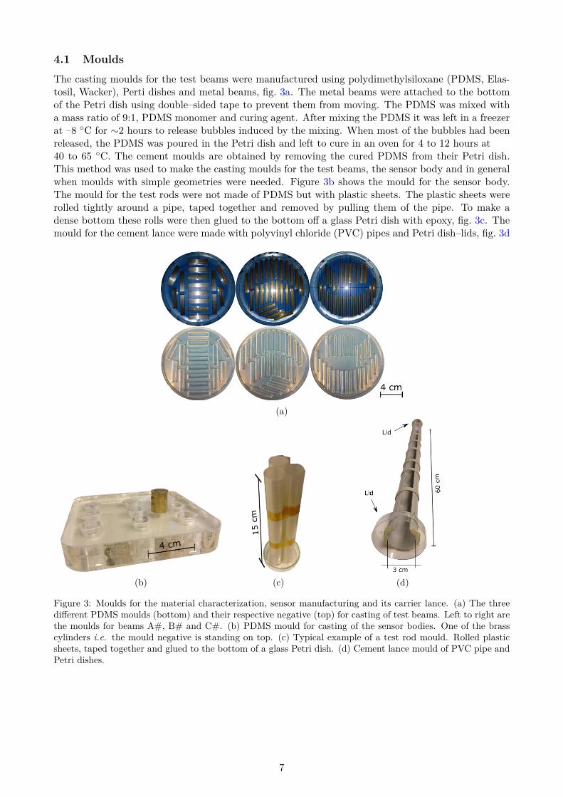
The casting moulds for the test beams were manufactured using polydimethylsiloxane (PDMS, Elas-tosil, Wacker), Perti dishes and metal beams, fig. 3a. The metal beams were attached to the bottomof the Petri dish using double–sided tape to prevent them from moving. The PDMS was mixed witha mass ratio of 9:1, PDMS monomer and curing agent. After mixing the PDMS it was left in a freezerat –8 C for ∼2 hours to release bubbles induced by the mixing. When most of the bubbles had beenreleased, the PDMS was poured in the Petri dish and left to cure in an oven for 4 to 12 hours at40 to 65 C. The cement moulds are obtained by removing the cured PDMS from their Petri dish.This method was used to make the casting moulds for the test beams, the sensor body and in generalwhen moulds with simple geometries were needed. Figure 3b shows the mould for the sensor body.The mould for the test rods were not made of PDMS but with plastic sheets. The plastic sheets wererolled tightly around a pipe, taped together and removed by pulling them of the pipe. To make adense bottom these rolls were then glued to the bottom off a glass Petri dish with epoxy, fig. 3c. Themould for the cement lance were made with polyvinyl chloride (PVC) pipes and Petri dish–lids, fig. 3d

(a)

(b) (c) (d)

Figure 3: Moulds for the material characterization, sensor manufacturing and its carrier lance. (a) The threedifferent PDMS moulds (bottom) and their respective negative (top) for casting of test beams. Left to right arethe moulds for beams A#, B# and C#. (b) PDMS mould for casting of the sensor bodies. One of the brasscylinders i.e. the mould negative is standing on top. (c) Typical example of a test rod mould. Rolled plasticsheets, taped together and glued to the bottom of a glass Petri dish. (d) Cement lance mould of PVC pipe andPetri dishes.

7

4.2 Casting

Since the properties and processing of this cement is partly unknown, several recipes needed to bedeveloped and evaluated. Parameters of interest, correlated to the particle size of the cement, aresurface roughness, mechanical properties and thermal shock resistance. The MiMix cement consists ofa mixture of particles of different sizes, where the largest particles are fairly large compared to normalcement. Portland cement has a particle size of 1.5 to 160 µm [25]. The largest particles of the Mimixcement are about 3 mm and the smallest as well as the and particle size distribution is unknown.For simplicity, the maximum particle size will be denoted pm from now on. To analyse the impact ofthe particle size, the original powder was divided into three separate batches. Batch A is the originalpowder with pm ≤3 mm, batch B has pm ≤1 mm and batch C has pm ≤0.4 mm.

A data sheet was provided with information about, e.g., the required water amount, table 1. Therewas little to no information about the mixing method which led to the development of own methods.The mixing was done by hand with a spoon in a plastic cup and with a food processor with 1200 Wof power (Electrolux Ultramix Professional EKM 9000). Batch A, B and C were mixed by hand witha w/c ratio of 8.05 wt%, 10.05 wt% and 13.30 wt%, respectively. Here, half of the cement powderwas added along with all the water, and mixed together until a homogeneous slurry was achieved.The rest of the cement was then added and mixed. The total cement amount varied from 50 to 100g. With the food processor, all the cement and water was added at once and mixed vigorously for 3minutes. Only batch A was mixed with the food processor and had a w/c ratio of 6.7 wt%. With thefood processor the total cement amount were 1 kg.

Table 1: Technical data of MiMix CA 97 Gk∗.

Product description Ceramic casting mix based on corundum withhydraulic bond

Application field Refractory lining of melting aggregates of high thermaland/or erosive attack

Chemical composition Material Amount [wt%]Alumina 97–98Lime and Magnesia 2.0–2.2Iron oxide < 0.1Alkali < 0.3

Water requirement Vibrating: 5.8–6.2 wt% Casting: 6.5–7.0 wt%Limiting application temperature 1800 CCold crushing strength 800 C/5h 57 N/mm2

1000 C/5h 52 N/mm2

1200 C/5h 73 N/mm2

1350 C/5h 130 N/mm2

Material requirement 2.9–3.0 t/m3

∗Part of data sheet from the manufacturer.

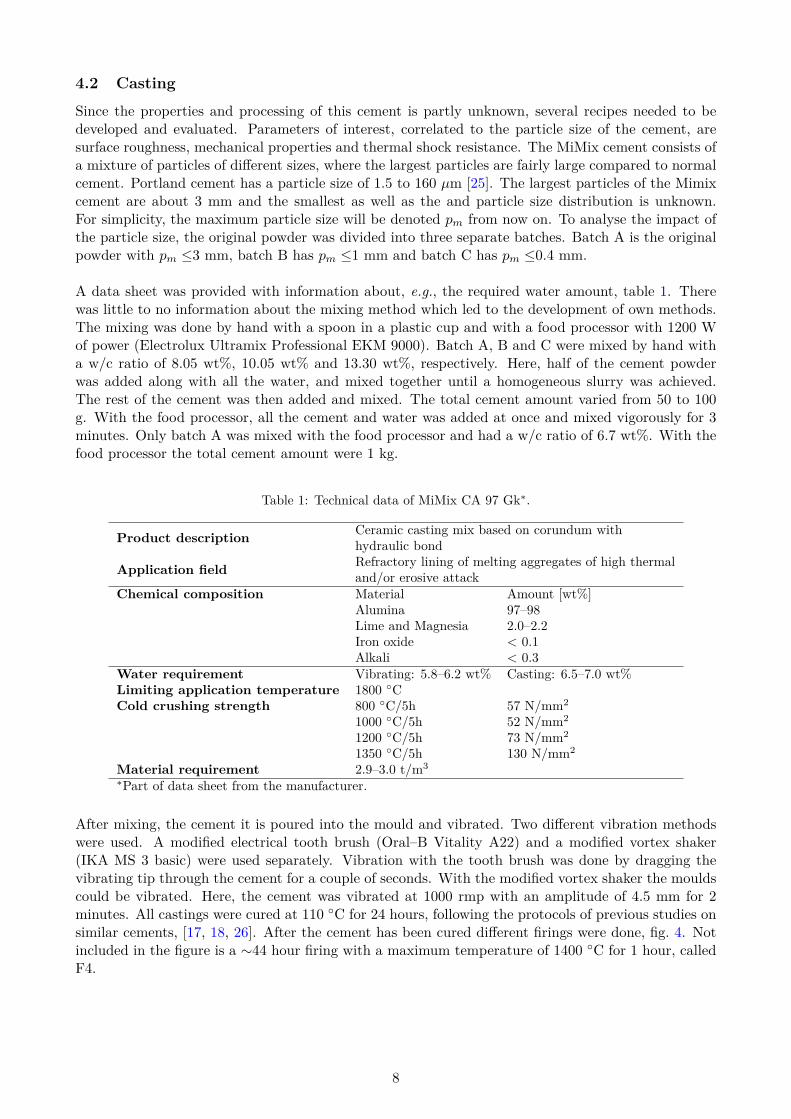
After mixing, the cement it is poured into the mould and vibrated. Two different vibration methodswere used. A modified electrical tooth brush (Oral–B Vitality A22) and a modified vortex shaker(IKA MS 3 basic) were used separately. Vibration with the tooth brush was done by dragging thevibrating tip through the cement for a couple of seconds. With the modified vortex shaker the mouldscould be vibrated. Here, the cement was vibrated at 1000 rmp with an amplitude of 4.5 mm for 2minutes. All castings were cured at 110 C for 24 hours, following the protocols of previous studies onsimilar cements, [17, 18, 26]. After the cement has been cured different firings were done, fig. 4. Notincluded in the figure is a ∼44 hour firing with a maximum temperature of 1400 C for 1 hour, calledF4.

8

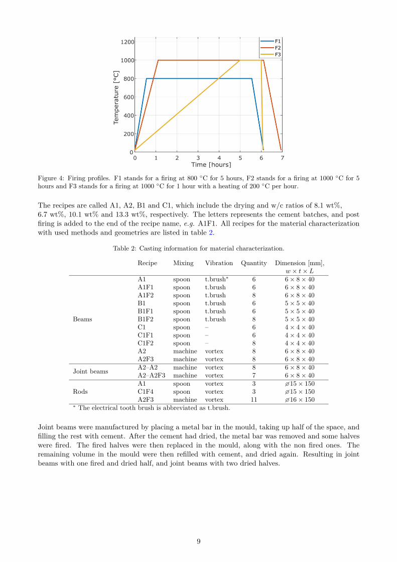
Figure 4: Firing profiles. F1 stands for a firing at 800 C for 5 hours, F2 stands for a firing at 1000 C for 5hours and F3 stands for a firing at 1000 C for 1 hour with a heating of 200 C per hour.

The recipes are called A1, A2, B1 and C1, which include the drying and w/c ratios of 8.1 wt%,6.7 wt%, 10.1 wt% and 13.3 wt%, respectively. The letters represents the cement batches, and postfiring is added to the end of the recipe name, e.g. A1F1. All recipes for the material characterizationwith used methods and geometries are listed in table 2.

Table 2: Casting information for material characterization.

Recipe Mixing Vibration Quantity Dimension [mm],w × t× L

Beams

A1 spoon t.brush∗ 6 6 × 8 × 40A1F1 spoon t.brush 6 6 × 8 × 40A1F2 spoon t.brush 8 6 × 8 × 40B1 spoon t.brush 6 5 × 5 × 40B1F1 spoon t.brush 6 5 × 5 × 40B1F2 spoon t.brush 8 5 × 5 × 40C1 spoon – 6 4 × 4 × 40C1F1 spoon – 6 4 × 4 × 40C1F2 spoon – 8 4 × 4 × 40A2 machine vortex 8 6 × 8 × 40A2F3 machine vortex 8 6 × 8 × 40

Joint beams A2–A2 machine vortex 8 6 × 8 × 40A2–A2F3 machine vortex 7 6 × 8 × 40

RodsA1 spoon vortex 3 15 × 150C1F4 spoon vortex 3 15 × 150A2F3 machine vortex 11 16 × 150

∗ The electrical tooth brush is abbreviated as t.brush.

Joint beams were manufactured by placing a metal bar in the mould, taking up half of the space, andfilling the rest with cement. After the cement had dried, the metal bar was removed and some halveswere fired. The fired halves were then replaced in the mould, along with the non fired ones. Theremaining volume in the mould were then refilled with cement, and dried again. Resulting in jointbeams with one fired and dried half, and joint beams with two dried halves.

9

4.3 Metallization process development

Printing on high–purity alumina tape, an HTCC material, with platinum paste (ESL 5571, ElectroScience Laboratories, USA) is well known from previous studies. When firing this system, it shrinksabout 20% at 1550 C. This is mostly due to the fact that the alumina tape contains organic compo-nents, which are burned away during firing. [27–29] As for the cement, this shrinkage will not occur.This fact, among other things, require a new metallization process to be developed.

As a first test, a left–over test beam was used as a substrate. The patterns chosen for printing wereof microthrusters, fig. 5, which had been used in a separate study at the university.

Figure 5: Microthruster pattern used in the metallization development.

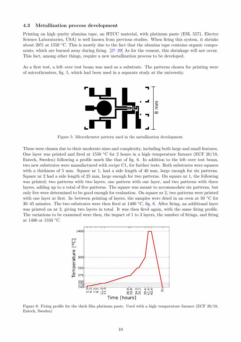
These were chosen due to their moderate sizes and complexity, including both large and small features.One layer was printed and fired at 1550 C for 2 hours in a high–temperature furnace (ECF 20/18,Entech, Sweden) following a profile much like that of fig. 6. In addition to the left–over test beam,two new substrates were manufactured with recipe C1, for further tests. Both substrates were squareswith a thickness of 5 mm. Square nr 1, had a side length of 40 mm, large enough for six patterns.Square nr 2 had a side length of 25 mm, large enough for two patterns. On square nr 1, the followingwas printed; two patterns with two layers, one pattern with one layer, and two patterns with threelayers, adding up to a total of five patterns. The square was meant to accommodate six patterns, butonly five were determined to be good enough for evaluation. On square nr 2, two patterns were printedwith one layer at first. In–between printing of layers, the samples were dried in an oven at 50 C for30–45 minutes. The two substrates were then fired at 1400 C, fig. 6. After firing, an additional layerwas printed on nr 2, giving two layers in total. It was then fired again, with the same firing profile.The variations to be examined were then, the impact of 1 to 3 layers, the number of firings, and firingat 1400 or 1550 C.

Figure 6: Firing profile for the thick film platinum paste. Used with a high–temperature furnace (ECF 20/18,Entech, Sweden)

10

4.3.1 Thick film characteristics

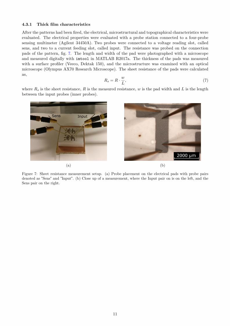
After the patterns had been fired, the electrical, microstructural and topographical characteristics wereevaluated. The electrical properties were evaluated with a probe station connected to a four-probesensing multimeter (Agilent 34450A). Two probes were connected to a voltage reading slot, calledsens, and two to a current feeding slot, called input. The resistance was probed on the connectionpads of the pattern, fig. 7. The length and width of the pad were photographed with a microscopeand measured digitally with imtool in MATLAB R2017a. The thickness of the pads was measuredwith a surface profiler (Veeco, Dektak 150), and the microstructure was examined with an opticalmicroscope (Olympus AX70 Research Microscope). The sheet resistance of the pads were calculatedas,

Rs = R · wL, (7)

where Rs is the sheet resistance, R is the measured resistance, w is the pad width and L is the lengthbetween the input probes (inner probes).

(a) (b)

Figure 7: Sheet resistance measurement setup. (a) Probe placement on the electrical pads with probe pairsdenoted as "Sens" and "Input". (b) Close up of a measurement, where the Input pair on is on the left, and theSens pair on the right.

11

4.4 Material characterization

4.4.1 Thermal shock

It is hard to thermally shock a material from hundreds of degrees to room temperature in a quick andcontrolled manner. A common way is to quench the specimen in water, with a known temperature[30]. Here, the beams were heated in two different ways but thermally shocked in the same way. TheA1, B1 and C1 beams were heated together with the furnace, to 1000 C, whereas the A1F1, A1F2,B1F1, B1F2, C1F1 and C1F2 ones were put in the furnace at 1000 C. It takes about 1 hour and45 minutes to heat the furnace to 1000 C. The temperatures was for the furnace between 1000 and1019 C, and the water bath of 16.0 and 22.5 C during the tests. All beams were put standing upin cylindrical crucibles with a depth of 4.5 cm, one crucible for each recipe. The crucible is mainly asample holder but also a heat shield, preventing inhomogeneous cooling on the beams upon extractionfrom the furnace. The crucibles were extracted one at a time with a pair of tongs and the beamswere quickly tipped out, down in a ∼2 litre container of water, from a hight of about 5 cm. Afterthe first crucible had been emptied, the furnace was closed again to be reheated, to acquire the sametemperature for the remaining beams. The A1F1, A1F2, B1F1, B1F2, C1F1 and C1F2 beams wereput in the hot furnace for 15, 7 and 5 minutes, respectively, before quenching. The thermal shockmethods are abbreviated as Ts1 and Ts2 for future referencing. Ts1 corresponds to a heating of thebeams with the furnace, and Ts2 corresponds to the beams being placed in a hot furnace.

4.4.2 Three–point beam bending

The casted and treated beams were analysed with a universal testing machine (SHIMADZU autographAGS–X) to obtain σf and Ef without and after thermal chock. A total of 91 beams were tested intotal, where 15 of them were the joint beams. The set–up of the experiment, fig. 8, was done withthe aid of ASTM C1161–13 standard. The span length was set to 22.5 mm on cylindrical supportswith a radius of 4.98 mm. The radius of the load cylinder was 4.00 mm and the displacement speedwas set to 0.2 mm per minute. Before placing the beams on the supports, the width and thicknessat the middle was measured. Before the measurement began, the loading arm was lowered to a pointwhere it was in contact with the beam, giving the beam a small pre–load. This was done to avoiddata points at the start which correspond to the movements in the test rig. For the joint beams theload cylinder was placed directly above the joint, at least within a fraction of the cylinder’s radius.

The mechanical properties, σf and Ef were calculated with the raw data, using eqs. (1) and (3) anda cross section of a A1 and C1 beam were analysed with EDS in SEM.

Figure 8: Close–up of the typical bending setup for one of the beams.

12

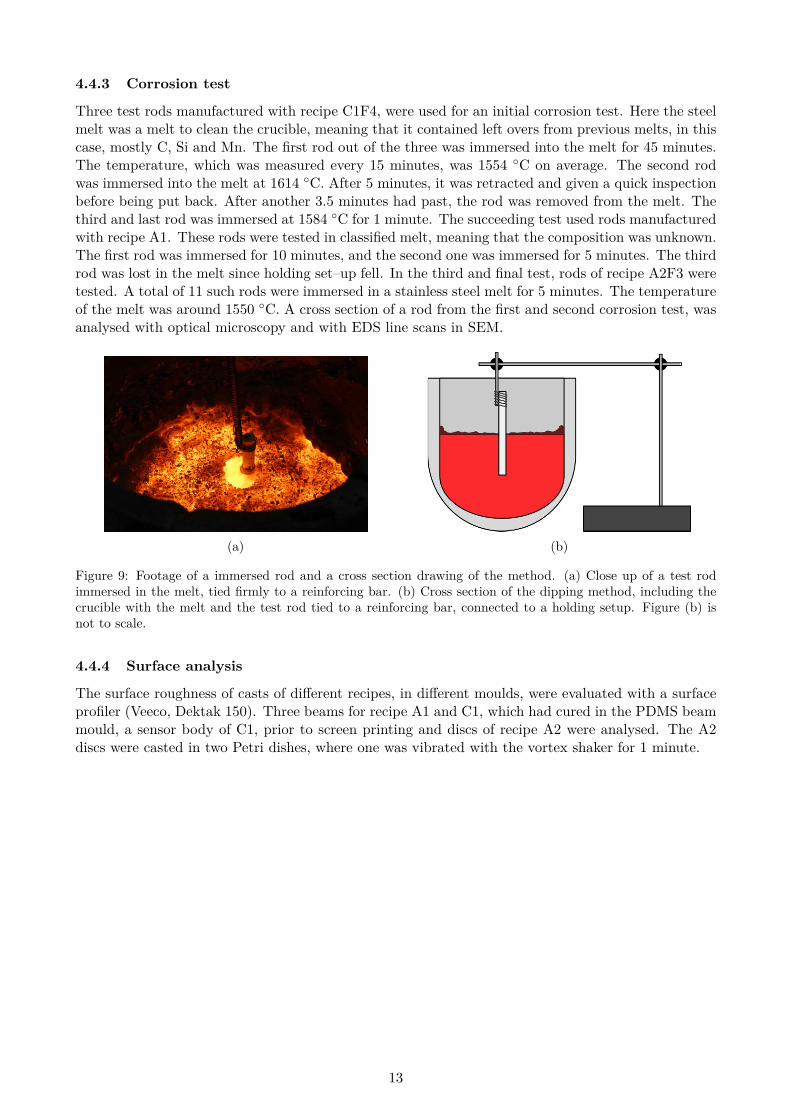
4.4.3 Corrosion test

Three test rods manufactured with recipe C1F4, were used for an initial corrosion test. Here the steelmelt was a melt to clean the crucible, meaning that it contained left overs from previous melts, in thiscase, mostly C, Si and Mn. The first rod out of the three was immersed into the melt for 45 minutes.The temperature, which was measured every 15 minutes, was 1554 C on average. The second rodwas immersed into the melt at 1614 C. After 5 minutes, it was retracted and given a quick inspectionbefore being put back. After another 3.5 minutes had past, the rod was removed from the melt. Thethird and last rod was immersed at 1584 C for 1 minute. The succeeding test used rods manufacturedwith recipe A1. These rods were tested in classified melt, meaning that the composition was unknown.The first rod was immersed for 10 minutes, and the second one was immersed for 5 minutes. The thirdrod was lost in the melt since holding set–up fell. In the third and final test, rods of recipe A2F3 weretested. A total of 11 such rods were immersed in a stainless steel melt for 5 minutes. The temperatureof the melt was around 1550 C. A cross section of a rod from the first and second corrosion test, wasanalysed with optical microscopy and with EDS line scans in SEM.

(a) (b)

Figure 9: Footage of a immersed rod and a cross section drawing of the method. (a) Close up of a test rodimmersed in the melt, tied firmly to a reinforcing bar. (b) Cross section of the dipping method, including thecrucible with the melt and the test rod tied to a reinforcing bar, connected to a holding setup. Figure (b) isnot to scale.

4.4.4 Surface analysis

The surface roughness of casts of different recipes, in different moulds, were evaluated with a surfaceprofiler (Veeco, Dektak 150). Three beams for recipe A1 and C1, which had cured in the PDMS beammould, a sensor body of C1, prior to screen printing and discs of recipe A2 were analysed. The A2discs were casted in two Petri dishes, where one was vibrated with the vortex shaker for 1 minute.

13

4.5 Sensor design

4.5.1 Sensor body

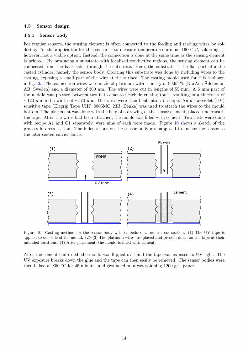
For regular sensors, the sensing element is often connected to the feeding and reading wires by sol-dering. As the application for this sensor is to measure temperatures around 1600 C, soldering is,however, not a viable option. Instead, the connection is done at the same time as the sensing elementis printed. By producing a substrate with localized conductive regions, the sensing element can beconnected from the back side, through the substrate. Here, the substrate is the flat part of a thecasted cylinder, namely the sensor body. Creating this substrate was done by including wires to thecasting, exposing a small part of the wire at the surface. The casting mould used for this is shownin fig. 3b. The connection wires were made of platinum with a purity of 99.95 % (KarAna ÄdelmetalAB, Sweden) and a diameter of 300 µm. The wires were cut in lengths of 55 mm. A 5 mm part ofthe middle was pressed between two flat cemented carbide cutting tools, resulting in a thickness of∼120 µm and a width of ∼570 µm. The wires were then bent into a U shape. An ultra–violet (UV)sensitive tape (Elegrip Tape UHP–0805MC–23B, Denka) was used to attach the wires to the mouldbottom. The placement was done with the help of a drawing of the sensor element, placed underneaththe tape. After the wires had been attached, the mould was filled with cement. Two casts were donewith recipe A1 and C1 separately, were nine of each were made. Figure 10 shows a sketch of theprocess in cross section. The indentations on the sensor body are supposed to anchor the sensor tothe later casted carrier lance.

Figure 10: Casting method for the sensor body with embedded wires in cross section. (1) The UV tape isapplied to one side of the mould. (2)–(3) The platinum wires are placed and pressed down on the tape at theirintended locations. (4) After placement, the mould is filled with cement.

After the cement had dried, the mould was flipped over and the tape was exposed to UV light. TheUV exposure breaks down the glue and the tape can then easily be removed. The sensor bodies werethen baked at 850 C for 45 minutes and grounded on a wet spinning 1200 grit paper.

14

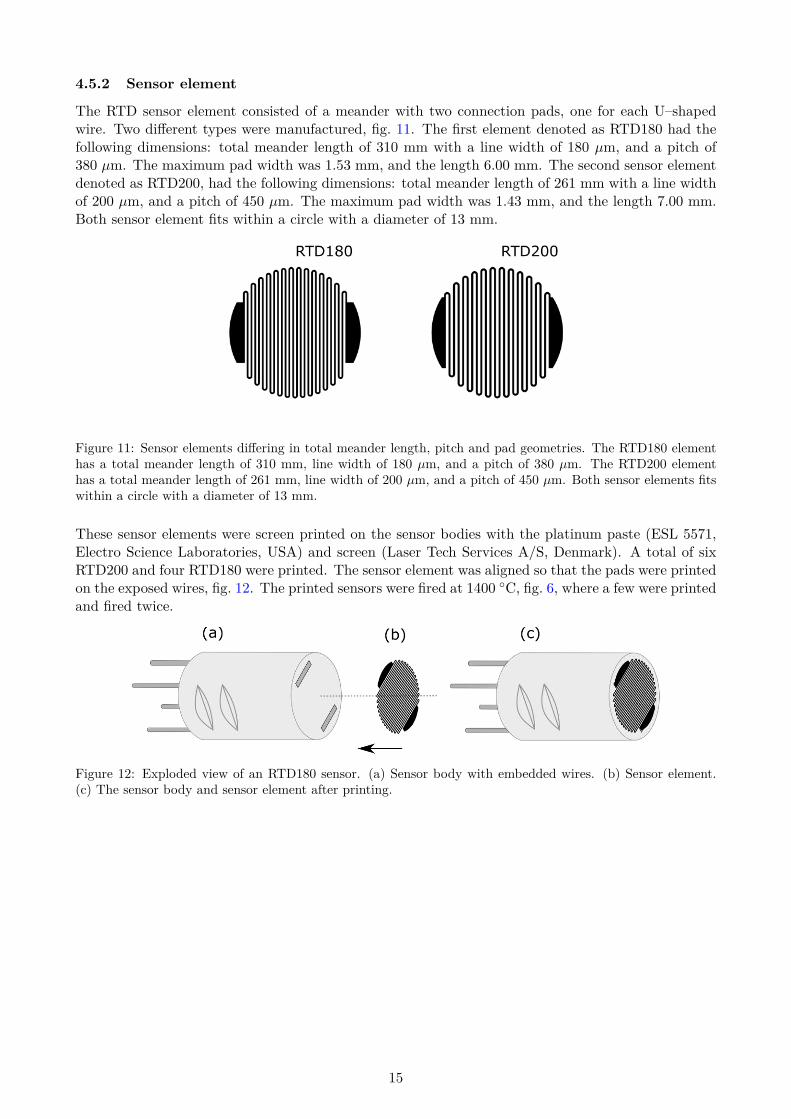
4.5.2 Sensor element

The RTD sensor element consisted of a meander with two connection pads, one for each U–shapedwire. Two different types were manufactured, fig. 11. The first element denoted as RTD180 had thefollowing dimensions: total meander length of 310 mm with a line width of 180 µm, and a pitch of380 µm. The maximum pad width was 1.53 mm, and the length 6.00 mm. The second sensor elementdenoted as RTD200, had the following dimensions: total meander length of 261 mm with a line widthof 200 µm, and a pitch of 450 µm. The maximum pad width was 1.43 mm, and the length 7.00 mm.Both sensor element fits within a circle with a diameter of 13 mm.

Figure 11: Sensor elements differing in total meander length, pitch and pad geometries. The RTD180 elementhas a total meander length of 310 mm, line width of 180 µm, and a pitch of 380 µm. The RTD200 elementhas a total meander length of 261 mm, line width of 200 µm, and a pitch of 450 µm. Both sensor elements fitswithin a circle with a diameter of 13 mm.

These sensor elements were screen printed on the sensor bodies with the platinum paste (ESL 5571,Electro Science Laboratories, USA) and screen (Laser Tech Services A/S, Denmark). A total of sixRTD200 and four RTD180 were printed. The sensor element was aligned so that the pads were printedon the exposed wires, fig. 12. The printed sensors were fired at 1400 C, fig. 6, where a few were printedand fired twice.

Figure 12: Exploded view of an RTD180 sensor. (a) Sensor body with embedded wires. (b) Sensor element.(c) The sensor body and sensor element after printing.

15

4.6 Lance systems

Two lance systems were manufactured. Firstly, a hollow Sialon lance was used, in which the sensorbody was placed, and lastly a solid cement lance was manufactured, where the sensor body wasembedded in the lance.

4.6.1 Sialon lance

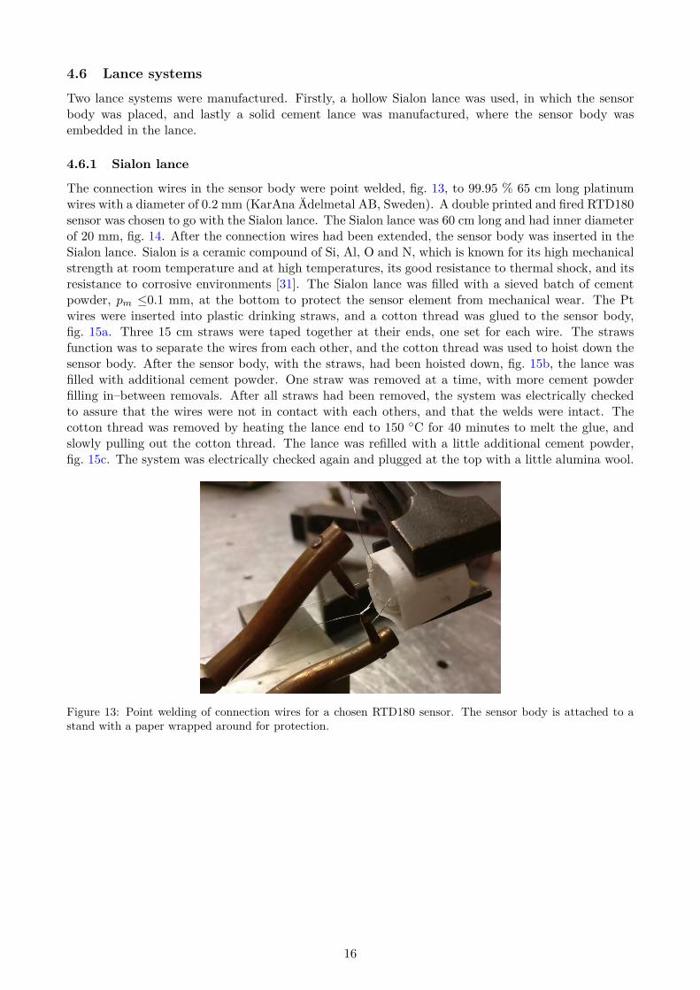
The connection wires in the sensor body were point welded, fig. 13, to 99.95 % 65 cm long platinumwires with a diameter of 0.2 mm (KarAna Ädelmetal AB, Sweden). A double printed and fired RTD180sensor was chosen to go with the Sialon lance. The Sialon lance was 60 cm long and had inner diameterof 20 mm, fig. 14. After the connection wires had been extended, the sensor body was inserted in theSialon lance. Sialon is a ceramic compound of Si, Al, O and N, which is known for its high mechanicalstrength at room temperature and at high temperatures, its good resistance to thermal shock, and itsresistance to corrosive environments [31]. The Sialon lance was filled with a sieved batch of cementpowder, pm ≤0.1 mm, at the bottom to protect the sensor element from mechanical wear. The Ptwires were inserted into plastic drinking straws, and a cotton thread was glued to the sensor body,fig. 15a. Three 15 cm straws were taped together at their ends, one set for each wire. The strawsfunction was to separate the wires from each other, and the cotton thread was used to hoist down thesensor body. After the sensor body, with the straws, had been hoisted down, fig. 15b, the lance wasfilled with additional cement powder. One straw was removed at a time, with more cement powderfilling in–between removals. After all straws had been removed, the system was electrically checkedto assure that the wires were not in contact with each others, and that the welds were intact. Thecotton thread was removed by heating the lance end to 150 C for 40 minutes to melt the glue, andslowly pulling out the cotton thread. The lance was refilled with a little additional cement powder,fig. 15c. The system was electrically checked again and plugged at the top with a little alumina wool.

Figure 13: Point welding of connection wires for a chosen RTD180 sensor. The sensor body is attached to astand with a paper wrapped around for protection.

16

Figure 14: Drawing of Sialon lance.

(a) (b) (c)

Figure 15: Wire separation and sensor body insertion. (a) Sensor body with plastic drinking straws coveringthe platinum wires and the red cotton thread glued to the sensor. (b) The sensor body has been hoisted downto the end of the lance. (c) Cross section after straws and thread have been removed.

17

4.6.2 Cement lance

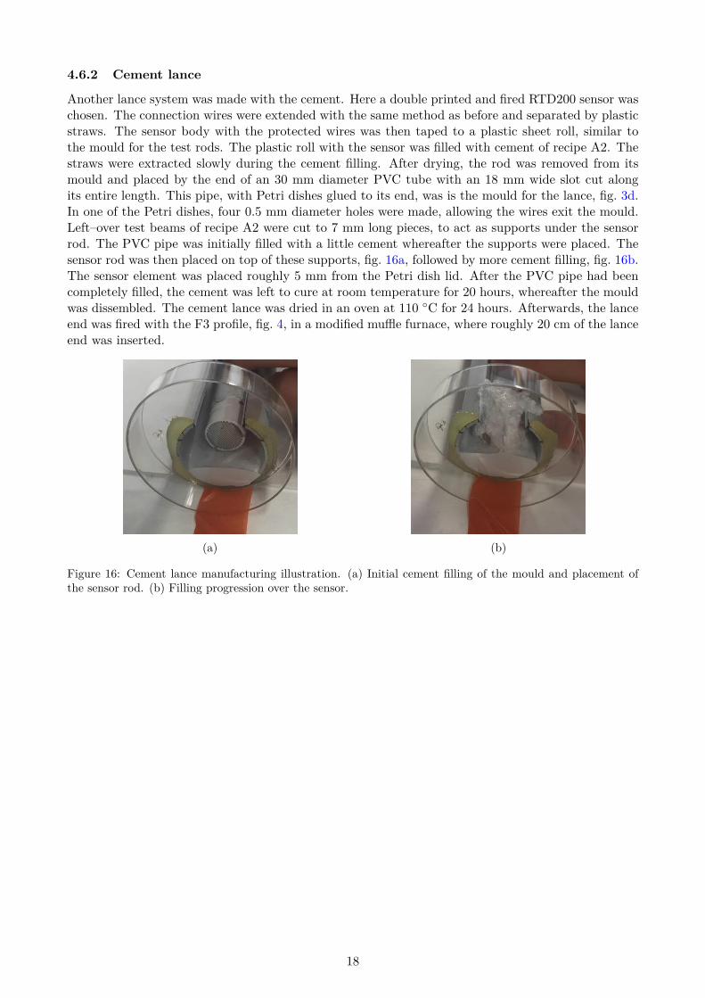
Another lance system was made with the cement. Here a double printed and fired RTD200 sensor waschosen. The connection wires were extended with the same method as before and separated by plasticstraws. The sensor body with the protected wires was then taped to a plastic sheet roll, similar tothe mould for the test rods. The plastic roll with the sensor was filled with cement of recipe A2. Thestraws were extracted slowly during the cement filling. After drying, the rod was removed from itsmould and placed by the end of an 30 mm diameter PVC tube with an 18 mm wide slot cut alongits entire length. This pipe, with Petri dishes glued to its end, was is the mould for the lance, fig. 3d.In one of the Petri dishes, four 0.5 mm diameter holes were made, allowing the wires exit the mould.Left–over test beams of recipe A2 were cut to 7 mm long pieces, to act as supports under the sensorrod. The PVC pipe was initially filled with a little cement whereafter the supports were placed. Thesensor rod was then placed on top of these supports, fig. 16a, followed by more cement filling, fig. 16b.The sensor element was placed roughly 5 mm from the Petri dish lid. After the PVC pipe had beencompletely filled, the cement was left to cure at room temperature for 20 hours, whereafter the mouldwas dissembled. The cement lance was dried in an oven at 110 C for 24 hours. Afterwards, the lanceend was fired with the F3 profile, fig. 4, in a modified muffle furnace, where roughly 20 cm of the lanceend was inserted.

(a) (b)

Figure 16: Cement lance manufacturing illustration. (a) Initial cement filling of the mould and placement ofthe sensor rod. (b) Filling progression over the sensor.

18

4.7 Sensor calibration

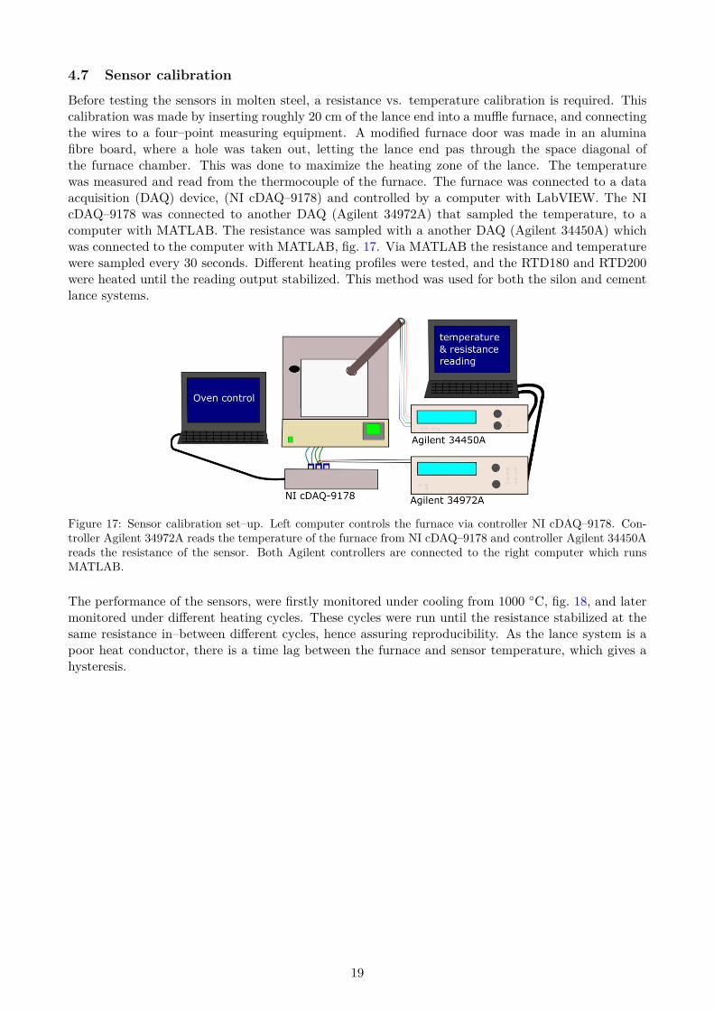
Before testing the sensors in molten steel, a resistance vs. temperature calibration is required. Thiscalibration was made by inserting roughly 20 cm of the lance end into a muffle furnace, and connectingthe wires to a four–point measuring equipment. A modified furnace door was made in an aluminafibre board, where a hole was taken out, letting the lance end pas through the space diagonal ofthe furnace chamber. This was done to maximize the heating zone of the lance. The temperaturewas measured and read from the thermocouple of the furnace. The furnace was connected to a dataacquisition (DAQ) device, (NI cDAQ–9178) and controlled by a computer with LabVIEW. The NIcDAQ–9178 was connected to another DAQ (Agilent 34972A) that sampled the temperature, to acomputer with MATLAB. The resistance was sampled with a another DAQ (Agilent 34450A) whichwas connected to the computer with MATLAB, fig. 17. Via MATLAB the resistance and temperaturewere sampled every 30 seconds. Different heating profiles were tested, and the RTD180 and RTD200were heated until the reading output stabilized. This method was used for both the silon and cementlance systems.

Figure 17: Sensor calibration set–up. Left computer controls the furnace via controller NI cDAQ–9178. Con-troller Agilent 34972A reads the temperature of the furnace from NI cDAQ–9178 and controller Agilent 34450Areads the resistance of the sensor. Both Agilent controllers are connected to the right computer which runsMATLAB.

The performance of the sensors, were firstly monitored under cooling from 1000 C, fig. 18, and latermonitored under different heating cycles. These cycles were run until the resistance stabilized at thesame resistance in–between different cycles, hence assuring reproducibility. As the lance system is apoor heat conductor, there is a time lag between the furnace and sensor temperature, which gives ahysteresis.

19

(a) (b)

Figure 18: Data acquired from first calibration cycle. (a) Resistance and temperature profile over a time of∼14 hours. (b) Resistance versus temperature hysteresis. Obtained by plotting the resistance against thetemperature from (a).

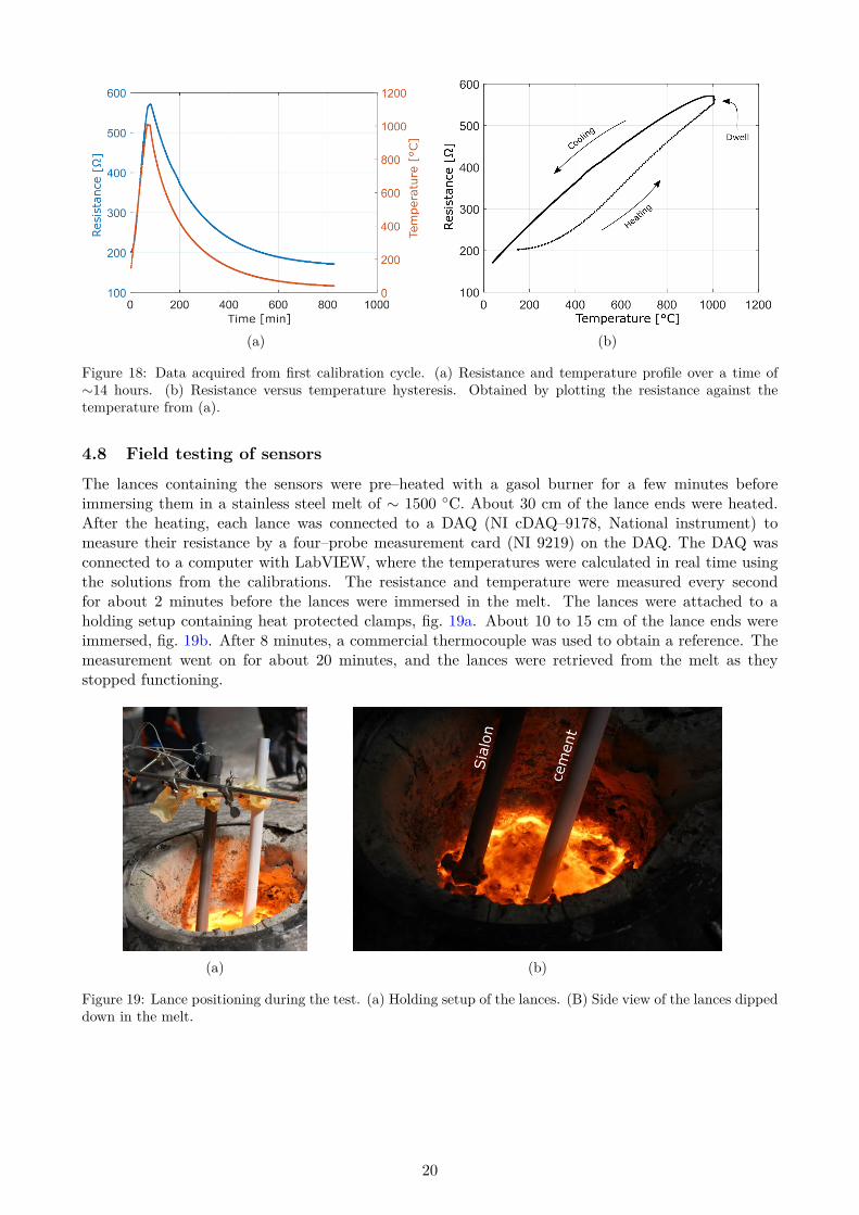
4.8 Field testing of sensors

The lances containing the sensors were pre–heated with a gasol burner for a few minutes beforeimmersing them in a stainless steel melt of ∼ 1500 C. About 30 cm of the lance ends were heated.After the heating, each lance was connected to a DAQ (NI cDAQ–9178, National instrument) tomeasure their resistance by a four–probe measurement card (NI 9219) on the DAQ. The DAQ wasconnected to a computer with LabVIEW, where the temperatures were calculated in real time usingthe solutions from the calibrations. The resistance and temperature were measured every secondfor about 2 minutes before the lances were immersed in the melt. The lances were attached to aholding setup containing heat protected clamps, fig. 19a. About 10 to 15 cm of the lance ends wereimmersed, fig. 19b. After 8 minutes, a commercial thermocouple was used to obtain a reference. Themeasurement went on for about 20 minutes, and the lances were retrieved from the melt as theystopped functioning.

(a) (b)

Figure 19: Lance positioning during the test. (a) Holding setup of the lances. (B) Side view of the lances dippeddown in the melt.

20

5 Results

5.1 Evaluation of metallization process

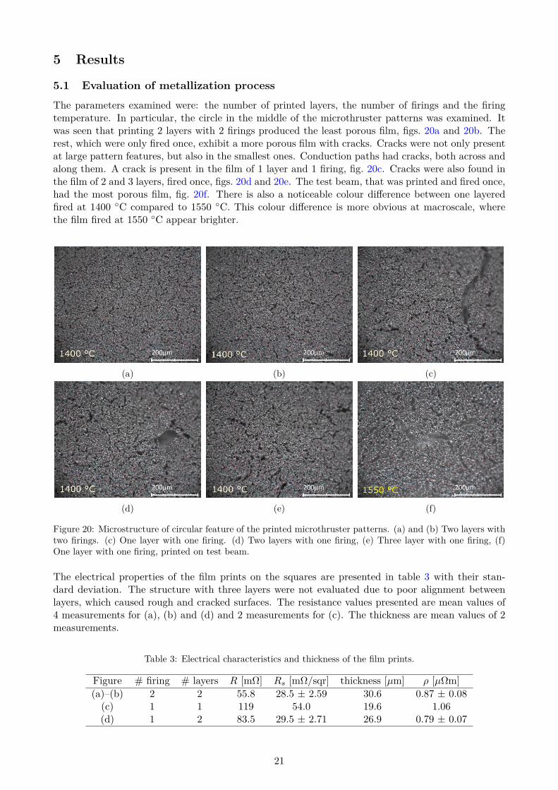
The parameters examined were: the number of printed layers, the number of firings and the firingtemperature. In particular, the circle in the middle of the microthruster patterns was examined. Itwas seen that printing 2 layers with 2 firings produced the least porous film, figs. 20a and 20b. Therest, which were only fired once, exhibit a more porous film with cracks. Cracks were not only presentat large pattern features, but also in the smallest ones. Conduction paths had cracks, both across andalong them. A crack is present in the film of 1 layer and 1 firing, fig. 20c. Cracks were also found inthe film of 2 and 3 layers, fired once, figs. 20d and 20e. The test beam, that was printed and fired once,had the most porous film, fig. 20f. There is also a noticeable colour difference between one layeredfired at 1400 C compared to 1550 C. This colour difference is more obvious at macroscale, wherethe film fired at 1550 C appear brighter.

(a) (b) (c)

(d) (e) (f)

Figure 20: Microstructure of circular feature of the printed microthruster patterns. (a) and (b) Two layers withtwo firings. (c) One layer with one firing. (d) Two layers with one firing, (e) Three layer with one firing, (f)One layer with one firing, printed on test beam.

The electrical properties of the film prints on the squares are presented in table 3 with their stan-dard deviation. The structure with three layers were not evaluated due to poor alignment betweenlayers, which caused rough and cracked surfaces. The resistance values presented are mean values of4 measurements for (a), (b) and (d) and 2 measurements for (c). The thickness are mean values of 2measurements.

Table 3: Electrical characteristics and thickness of the film prints.

Figure # firing # layers R [mΩ] Rs [mΩ/sqr] thickness [µm] ρ [µΩm](a)–(b) 2 2 55.8 28.5 ± 2.59 30.6 0.87 ± 0.08(c) 1 1 119 54.0 19.6 1.06(d) 1 2 83.5 29.5 ± 2.71 26.9 0.79 ± 0.07

21

5.2 Material properties

5.2.1 Bending strength

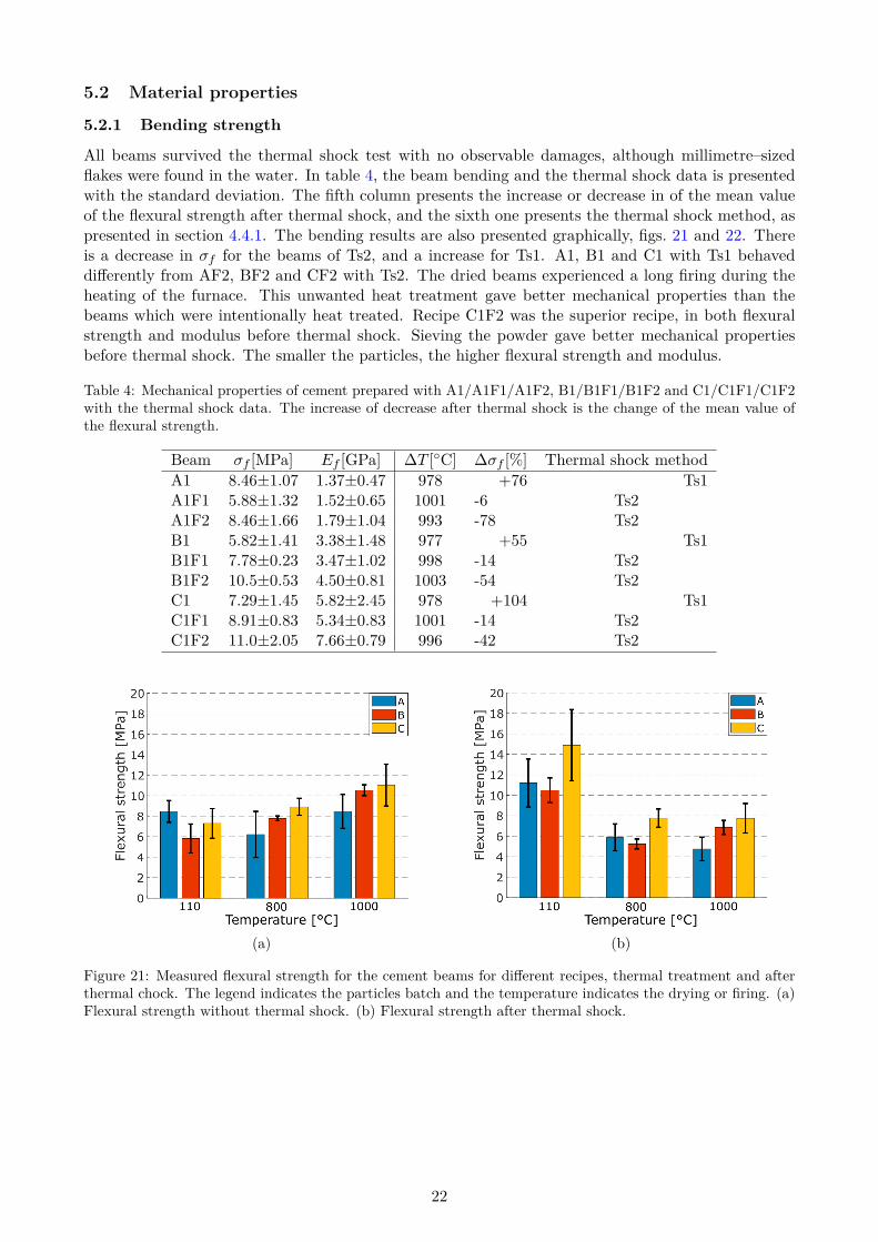
All beams survived the thermal shock test with no observable damages, although millimetre–sizedflakes were found in the water. In table 4, the beam bending and the thermal shock data is presentedwith the standard deviation. The fifth column presents the increase or decrease in of the mean valueof the flexural strength after thermal shock, and the sixth one presents the thermal shock method, aspresented in section 4.4.1. The bending results are also presented graphically, figs. 21 and 22. Thereis a decrease in σf for the beams of Ts2, and a increase for Ts1. A1, B1 and C1 with Ts1 behaveddifferently from AF2, BF2 and CF2 with Ts2. The dried beams experienced a long firing during theheating of the furnace. This unwanted heat treatment gave better mechanical properties than thebeams which were intentionally heat treated. Recipe C1F2 was the superior recipe, in both flexuralstrength and modulus before thermal shock. Sieving the powder gave better mechanical propertiesbefore thermal shock. The smaller the particles, the higher flexural strength and modulus.

Table 4: Mechanical properties of cement prepared with A1/A1F1/A1F2, B1/B1F1/B1F2 and C1/C1F1/C1F2with the thermal shock data. The increase of decrease after thermal shock is the change of the mean value ofthe flexural strength.

Beam σf [MPa] Ef [GPa] ∆T [C] ∆σf [%] Thermal shock methodA1 8.46±1.07 1.37±0.47 978 +76 Ts1A1F1 5.88±1.32 1.52±0.65 1001 -6 Ts2A1F2 8.46±1.66 1.79±1.04 993 -78 Ts2B1 5.82±1.41 3.38±1.48 977 +55 Ts1B1F1 7.78±0.23 3.47±1.02 998 -14 Ts2B1F2 10.5±0.53 4.50±0.81 1003 -54 Ts2C1 7.29±1.45 5.82±2.45 978 +104 Ts1C1F1 8.91±0.83 5.34±0.83 1001 -14 Ts2C1F2 11.0±2.05 7.66±0.79 996 -42 Ts2

(a) (b)

Figure 21: Measured flexural strength for the cement beams for different recipes, thermal treatment and afterthermal chock. The legend indicates the particles batch and the temperature indicates the drying or firing. (a)Flexural strength without thermal shock. (b) Flexural strength after thermal shock.

22

(a) (b)

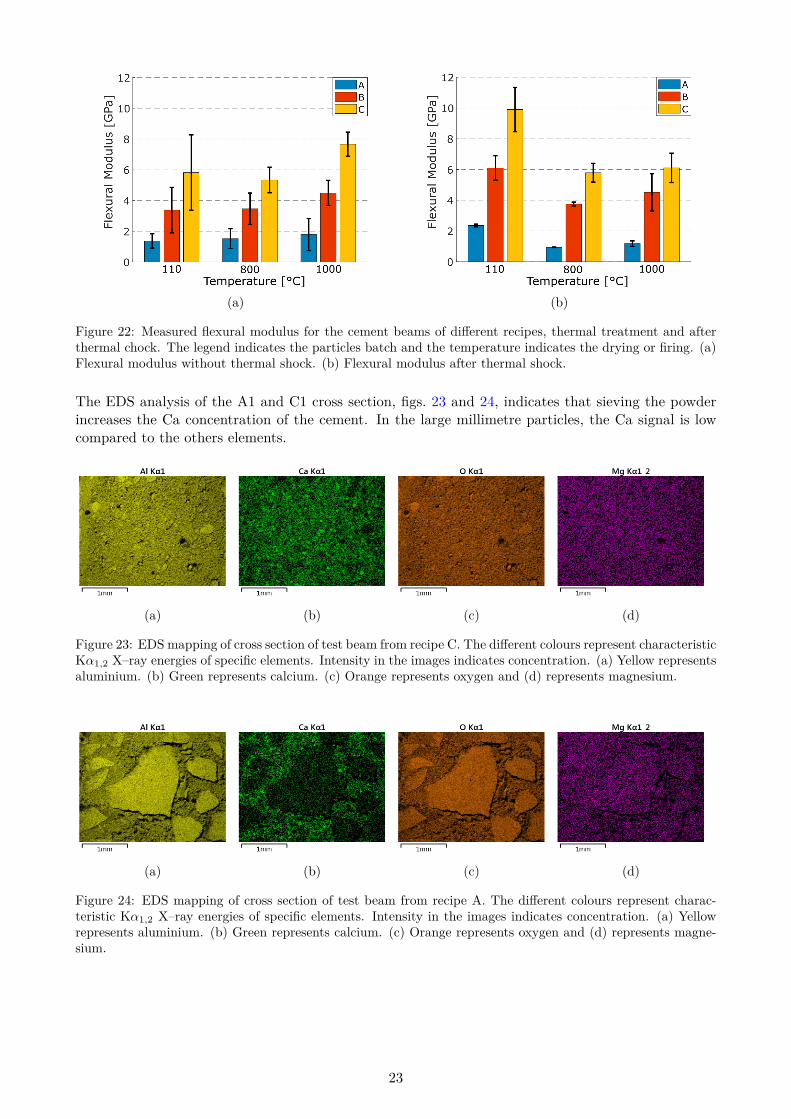
Figure 22: Measured flexural modulus for the cement beams of different recipes, thermal treatment and afterthermal chock. The legend indicates the particles batch and the temperature indicates the drying or firing. (a)Flexural modulus without thermal shock. (b) Flexural modulus after thermal shock.

The EDS analysis of the A1 and C1 cross section, figs. 23 and 24, indicates that sieving the powderincreases the Ca concentration of the cement. In the large millimetre particles, the Ca signal is lowcompared to the others elements.

(a) (b) (c) (d)

Figure 23: EDS mapping of cross section of test beam from recipe C. The different colours represent characteristicKα1,2 X–ray energies of specific elements. Intensity in the images indicates concentration. (a) Yellow representsaluminium. (b) Green represents calcium. (c) Orange represents oxygen and (d) represents magnesium.

(a) (b) (c) (d)

Figure 24: EDS mapping of cross section of test beam from recipe A. The different colours represent charac-teristic Kα1,2 X–ray energies of specific elements. Intensity in the images indicates concentration. (a) Yellowrepresents aluminium. (b) Green represents calcium. (c) Orange represents oxygen and (d) represents magne-sium.

23

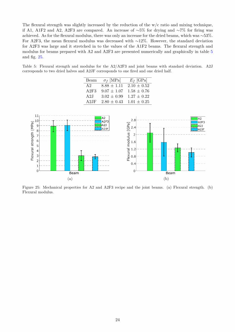
The flexural strength was slightly increased by the reduction of the w/c ratio and mixing technique,if A1, A1F2 and A2, A2F3 are compared. An increase of ∼5% for drying and ∼7% for firing wasachieved. As for the flexural modulus, there was only an increase for the dried beams, which was ∼53%.For A2F3, the mean flexural modulus was decreased with ∼12%. However, the standard deviationfor A2F3 was large and it stretched in to the values of the A1F2 beams. The flexural strength andmodulus for beams prepared with A2 and A2F3 are presented numerically and graphically in table 5and fig. 25.

Table 5: Flexural strength and modulus for the A2/A2F3 and joint beams with standard deviation. A2Jcorresponds to two dried halves and A2JF corresponds to one fired and one dried half.

Beam σf [MPa] Ef [GPa]A2 8.88 ± 1.11 2.10 ± 0.52A2F3 9.07 ± 1.07 1.58 ± 0.76A2J 3.02 ± 0.99 1.27 ± 0.22A2JF 2.80 ± 0.43 1.01 ± 0.25

(a) (b)

Figure 25: Mechanical properties for A2 and A2F3 recipe and the joint beams. (a) Flexural strength. (b)Flexural modulus.

24

5.2.2 Corrosion test of rods

This section presents the results of the corrosion tests described in section 4.4.3 for the test rods.Seventeen rods in total were tested at Sandvik, each recipe at different times and in different steelmelts. Afterwards, the rods were either cracked or cut open for observation of the cross section.

5.2.2.1 First test rods

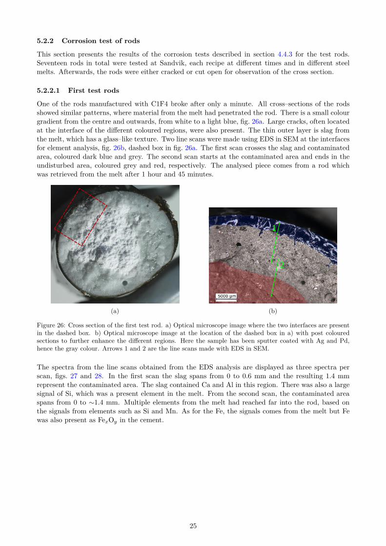
One of the rods manufactured with C1F4 broke after only a minute. All cross–sections of the rodsshowed similar patterns, where material from the melt had penetrated the rod. There is a small colourgradient from the centre and outwards, from white to a light blue, fig. 26a. Large cracks, often locatedat the interface of the different coloured regions, were also present. The thin outer layer is slag fromthe melt, which has a glass–like texture. Two line scans were made using EDS in SEM at the interfacesfor element analysis, fig. 26b, dashed box in fig. 26a. The first scan crosses the slag and contaminatedarea, coloured dark blue and grey. The second scan starts at the contaminated area and ends in theundisturbed area, coloured grey and red, respectively. The analysed piece comes from a rod whichwas retrieved from the melt after 1 hour and 45 minutes.

(a) (b)

Figure 26: Cross section of the first test rod. a) Optical microscope image where the two interfaces are presentin the dashed box. b) Optical microscope image at the location of the dashed box in a) with post colouredsections to further enhance the different regions. Here the sample has been sputter coated with Ag and Pd,hence the gray colour. Arrows 1 and 2 are the line scans made with EDS in SEM.

The spectra from the line scans obtained from the EDS analysis are displayed as three spectra perscan, figs. 27 and 28. In the first scan the slag spans from 0 to 0.6 mm and the resulting 1.4 mmrepresent the contaminated area. The slag contained Ca and Al in this region. There was also a largesignal of Si, which was a present element in the melt. From the second scan, the contaminated areaspans from 0 to ∼1.4 mm. Multiple elements from the melt had reached far into the rod, based onthe signals from elements such as Si and Mn. As for the Fe, the signals comes from the melt but Fewas also present as FexOy in the cement.

25

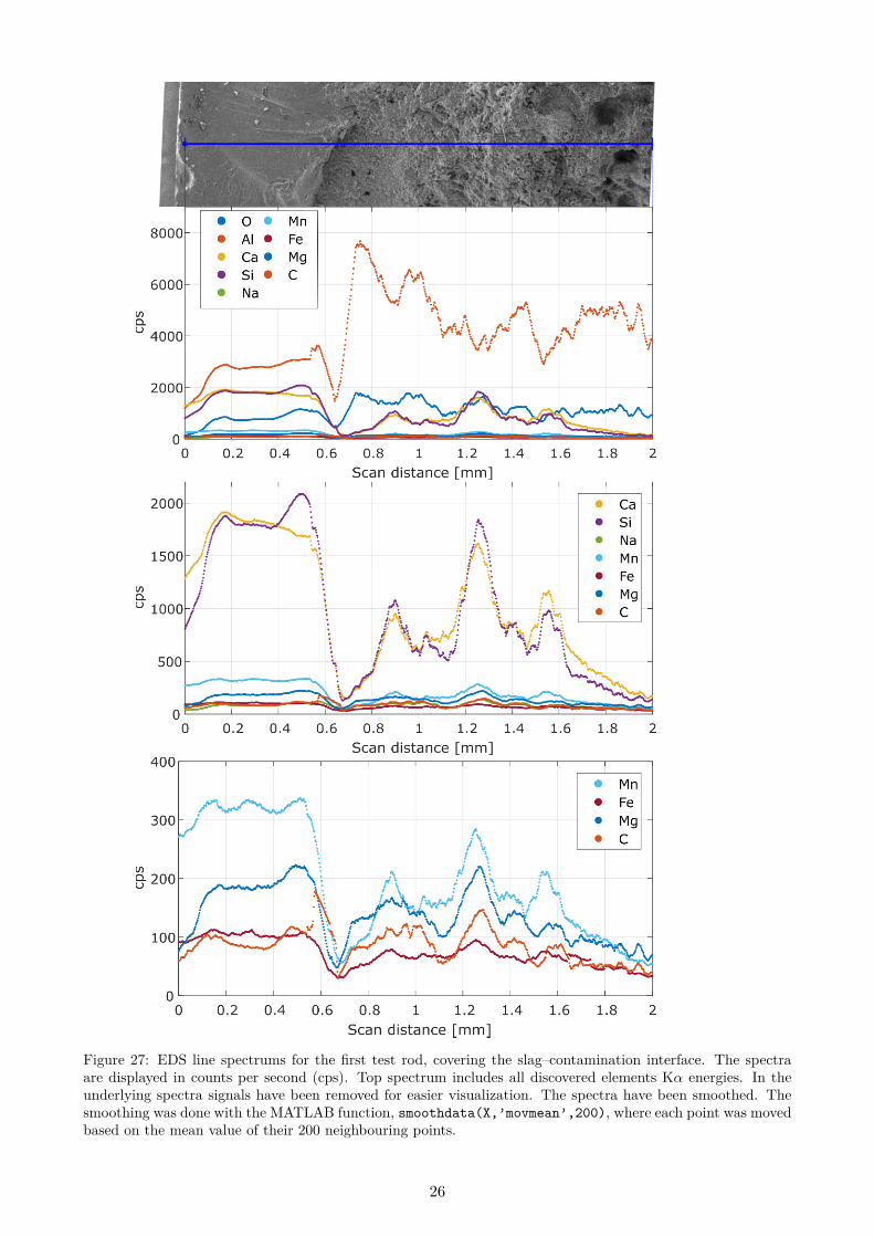
Figure 27: EDS line spectrums for the first test rod, covering the slag–contamination interface. The spectraare displayed in counts per second (cps). Top spectrum includes all discovered elements Kα energies. In theunderlying spectra signals have been removed for easier visualization. The spectra have been smoothed. Thesmoothing was done with the MATLAB function, smoothdata(X,’movmean’,200), where each point was movedbased on the mean value of their 200 neighbouring points.

26

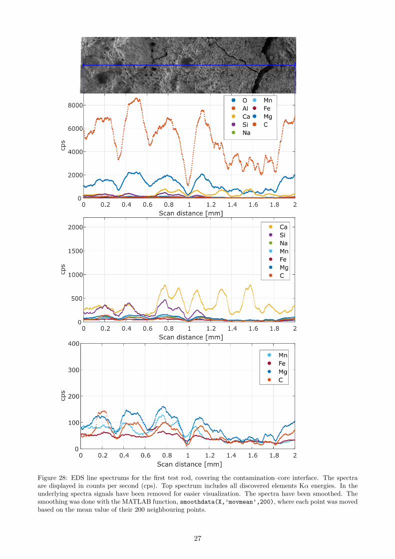
Figure 28: EDS line spectrums for the first test rod, covering the contamination–core interface. The spectraare displayed in counts per second (cps). Top spectrum includes all discovered elements Kα energies. In theunderlying spectra signals have been removed for easier visualization. The spectra have been smoothed. Thesmoothing was done with the MATLAB function, smoothdata(X,’movmean’,200), where each point was movedbased on the mean value of their 200 neighbouring points.

27

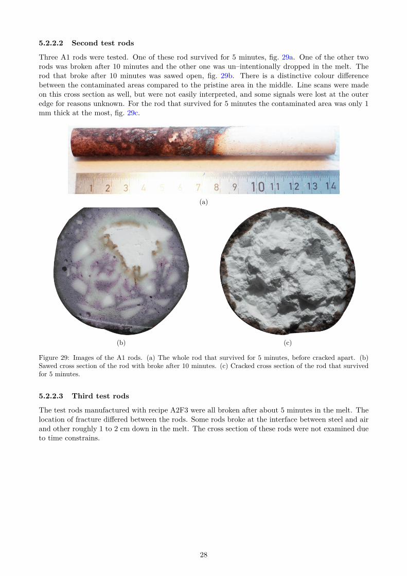
5.2.2.2 Second test rods

Three A1 rods were tested. One of these rod survived for 5 minutes, fig. 29a. One of the other tworods was broken after 10 minutes and the other one was un–intentionally dropped in the melt. Therod that broke after 10 minutes was sawed open, fig. 29b. There is a distinctive colour differencebetween the contaminated areas compared to the pristine area in the middle. Line scans were madeon this cross section as well, but were not easily interpreted, and some signals were lost at the outeredge for reasons unknown. For the rod that survived for 5 minutes the contaminated area was only 1mm thick at the most, fig. 29c.

(a)

(b) (c)

Figure 29: Images of the A1 rods. (a) The whole rod that survived for 5 minutes, before cracked apart. (b)Sawed cross section of the rod with broke after 10 minutes. (c) Cracked cross section of the rod that survivedfor 5 minutes.

5.2.2.3 Third test rods

The test rods manufactured with recipe A2F3 were all broken after about 5 minutes in the melt. Thelocation of fracture differed between the rods. Some rods broke at the interface between steel and airand other roughly 1 to 2 cm down in the melt. The cross section of these rods were not examined dueto time constrains.

28

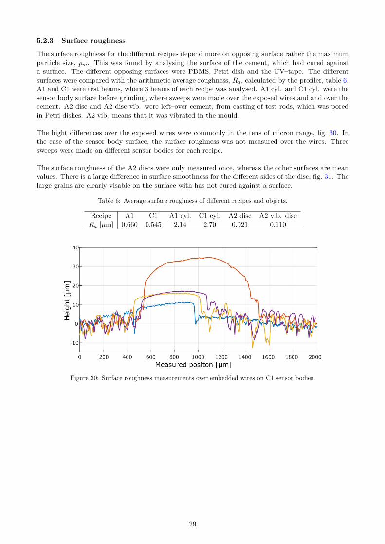
5.2.3 Surface roughness

The surface roughness for the different recipes depend more on opposing surface rather the maximumparticle size, pm. This was found by analysing the surface of the cement, which had cured againsta surface. The different opposing surfaces were PDMS, Petri dish and the UV–tape. The differentsurfaces were compared with the arithmetic average roughness, Ra, calculated by the profiler, table 6.A1 and C1 were test beams, where 3 beams of each recipe was analysed. A1 cyl. and C1 cyl. were thesensor body surface before grinding, where sweeps were made over the exposed wires and and over thecement. A2 disc and A2 disc vib. were left–over cement, from casting of test rods, which was poredin Petri dishes. A2 vib. means that it was vibrated in the mould.

The hight differences over the exposed wires were commonly in the tens of micron range, fig. 30. Inthe case of the sensor body surface, the surface roughness was not measured over the wires. Threesweeps were made on different sensor bodies for each recipe.

The surface roughness of the A2 discs were only measured once, whereas the other surfaces are meanvalues. There is a large difference in surface smoothness for the different sides of the disc, fig. 31. Thelarge grains are clearly visable on the surface with has not cured against a surface.

Table 6: Average surface roughness of different recipes and objects.

Recipe A1 C1 A1 cyl. C1 cyl. A2 disc A2 vib. discRa [µm] 0.660 0.545 2.14 2.70 0.021 0.110

Figure 30: Surface roughness measurements over embedded wires on C1 sensor bodies.

29

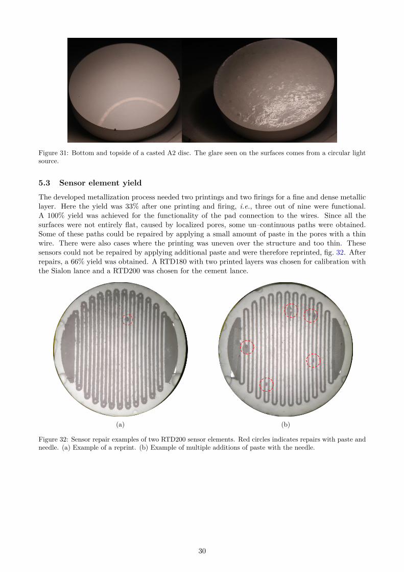
Figure 31: Bottom and topside of a casted A2 disc. The glare seen on the surfaces comes from a circular lightsource.

5.3 Sensor element yield

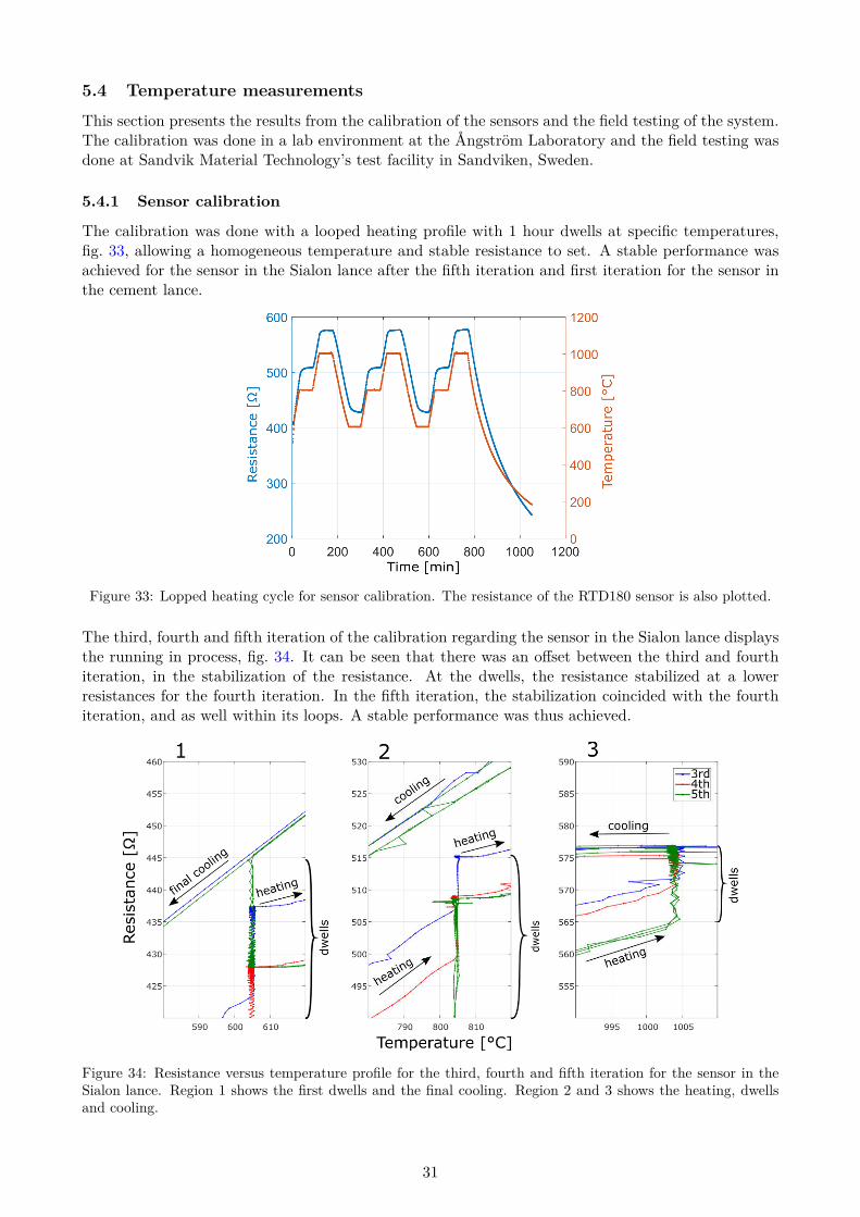
The developed metallization process needed two printings and two firings for a fine and dense metalliclayer. Here the yield was 33% after one printing and firing, i.e., three out of nine were functional.A 100% yield was achieved for the functionality of the pad connection to the wires. Since all thesurfaces were not entirely flat, caused by localized pores, some un–continuous paths were obtained.Some of these paths could be repaired by applying a small amount of paste in the pores with a thinwire. There were also cases where the printing was uneven over the structure and too thin. Thesesensors could not be repaired by applying additional paste and were therefore reprinted, fig. 32. Afterrepairs, a 66% yield was obtained. A RTD180 with two printed layers was chosen for calibration withthe Sialon lance and a RTD200 was chosen for the cement lance.

(a) (b)

Figure 32: Sensor repair examples of two RTD200 sensor elements. Red circles indicates repairs with paste andneedle. (a) Example of a reprint. (b) Example of multiple additions of paste with the needle.

30

5.4 Temperature measurements

This section presents the results from the calibration of the sensors and the field testing of the system.The calibration was done in a lab environment at the Ångström Laboratory and the field testing wasdone at Sandvik Material Technology’s test facility in Sandviken, Sweden.

5.4.1 Sensor calibration

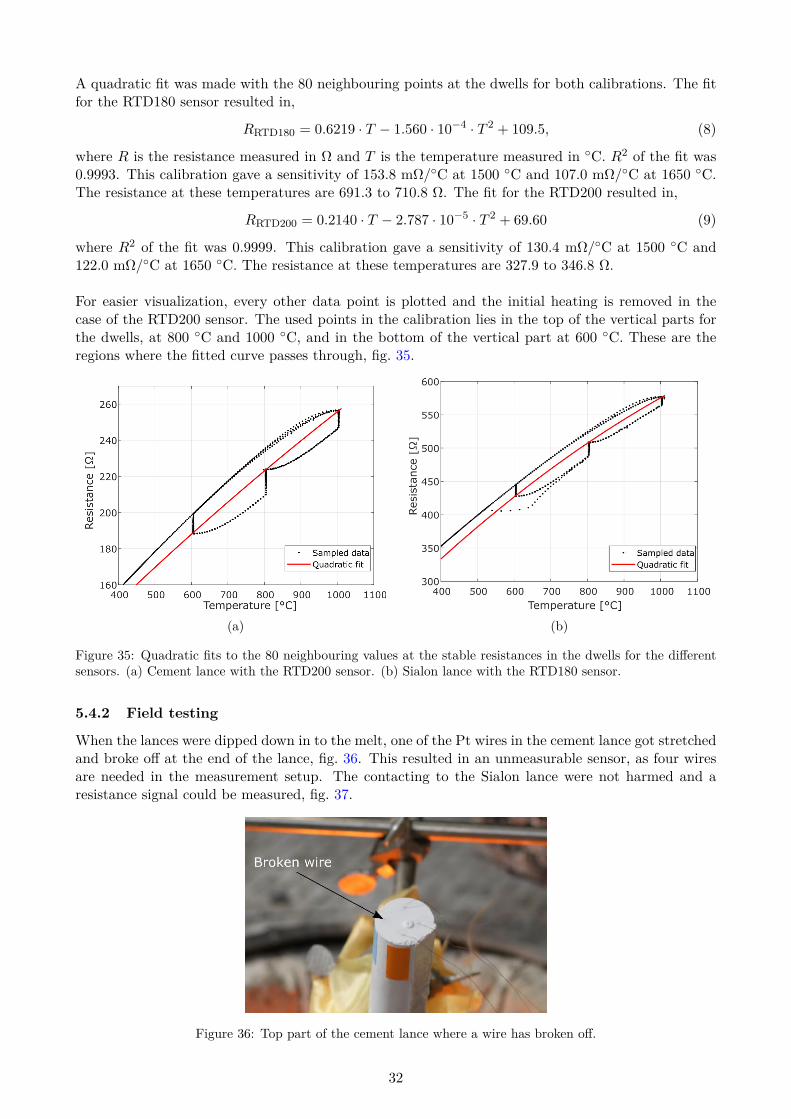
The calibration was done with a looped heating profile with 1 hour dwells at specific temperatures,fig. 33, allowing a homogeneous temperature and stable resistance to set. A stable performance wasachieved for the sensor in the Sialon lance after the fifth iteration and first iteration for the sensor inthe cement lance.

Figure 33: Lopped heating cycle for sensor calibration. The resistance of the RTD180 sensor is also plotted.

The third, fourth and fifth iteration of the calibration regarding the sensor in the Sialon lance displaysthe running in process, fig. 34. It can be seen that there was an offset between the third and fourthiteration, in the stabilization of the resistance. At the dwells, the resistance stabilized at a lowerresistances for the fourth iteration. In the fifth iteration, the stabilization coincided with the fourthiteration, and as well within its loops. A stable performance was thus achieved.

Figure 34: Resistance versus temperature profile for the third, fourth and fifth iteration for the sensor in theSialon lance. Region 1 shows the first dwells and the final cooling. Region 2 and 3 shows the heating, dwellsand cooling.

31

A quadratic fit was made with the 80 neighbouring points at the dwells for both calibrations. The fitfor the RTD180 sensor resulted in,

RRTD180 = 0.6219 · T − 1.560 · 10−4 · T 2 + 109.5, (8)

where R is the resistance measured in Ω and T is the temperature measured in C. R2 of the fit was0.9993. This calibration gave a sensitivity of 153.8 mΩ/C at 1500 C and 107.0 mΩ/C at 1650 C.The resistance at these temperatures are 691.3 to 710.8 Ω. The fit for the RTD200 resulted in,

RRTD200 = 0.2140 · T − 2.787 · 10−5 · T 2 + 69.60 (9)

where R2 of the fit was 0.9999. This calibration gave a sensitivity of 130.4 mΩ/C at 1500 C and122.0 mΩ/C at 1650 C. The resistance at these temperatures are 327.9 to 346.8 Ω.

For easier visualization, every other data point is plotted and the initial heating is removed in thecase of the RTD200 sensor. The used points in the calibration lies in the top of the vertical parts forthe dwells, at 800 C and 1000 C, and in the bottom of the vertical part at 600 C. These are theregions where the fitted curve passes through, fig. 35.

(a) (b)

Figure 35: Quadratic fits to the 80 neighbouring values at the stable resistances in the dwells for the differentsensors. (a) Cement lance with the RTD200 sensor. (b) Sialon lance with the RTD180 sensor.

5.4.2 Field testing

When the lances were dipped down in to the melt, one of the Pt wires in the cement lance got stretchedand broke off at the end of the lance, fig. 36. This resulted in an unmeasurable sensor, as four wiresare needed in the measurement setup. The contacting to the Sialon lance were not harmed and aresistance signal could be measured, fig. 37.

Figure 36: Top part of the cement lance where a wire has broken off.

32

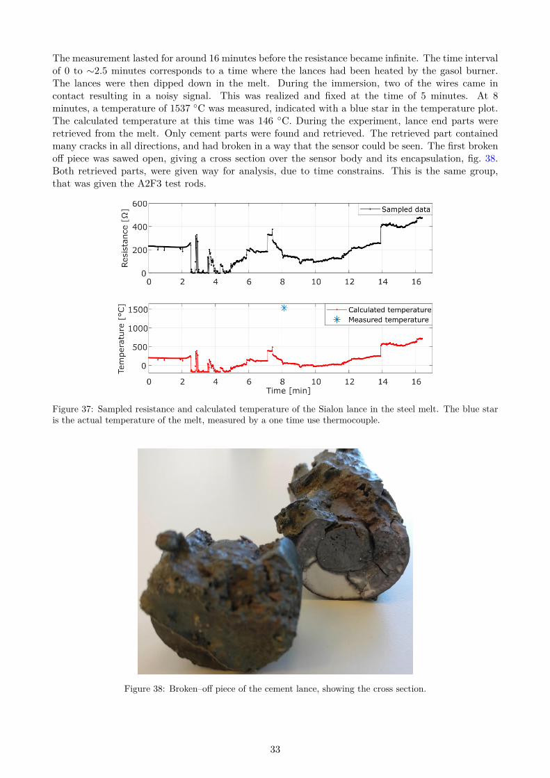
The measurement lasted for around 16 minutes before the resistance became infinite. The time intervalof 0 to ∼2.5 minutes corresponds to a time where the lances had been heated by the gasol burner.The lances were then dipped down in the melt. During the immersion, two of the wires came incontact resulting in a noisy signal. This was realized and fixed at the time of 5 minutes. At 8minutes, a temperature of 1537 C was measured, indicated with a blue star in the temperature plot.The calculated temperature at this time was 146 C. During the experiment, lance end parts wereretrieved from the melt. Only cement parts were found and retrieved. The retrieved part containedmany cracks in all directions, and had broken in a way that the sensor could be seen. The first brokenoff piece was sawed open, giving a cross section over the sensor body and its encapsulation, fig. 38.Both retrieved parts, were given way for analysis, due to time constrains. This is the same group,that was given the A2F3 test rods.

Figure 37: Sampled resistance and calculated temperature of the Sialon lance in the steel melt. The blue staris the actual temperature of the melt, measured by a one time use thermocouple.

Figure 38: Broken–off piece of the cement lance, showing the cross section.

33

6 Discussion

6.1 Processing

The casting of the cement proved to be more sensitive to the mixing method than expected. To achievethe recommended w/c ratios a powerful mixer was required. Mixing the cement by hand was not aviable option. To get a homogeneous mixture, the w/c ratio was increased stepwise from 5.8 to 13.3wt%. At too low w/c ratios, the cement was only partially wetted. The cement mixed with waterbehaves as a dilatant fluid, which is the main reason why it is so difficult to mix. As well as that thew/c ratios were small.

It was believed that the reduction of the w/c ratio and the new F4 firing profile would give the cementa better chemical resistance to the melt and better mechanical properties, causing it not to fracture, asthis cement is normally used in these environments. In previous experiments, parts of cement cruciblesfrom the manufacturer have been tested in steel melts with good results. It is difficult to determinewhich critical part in the processing is. The only known difference is that the manufacturer directlyheat treats the cement after casting, whereas here it was first dried and then fired. Moreover, thecement has recently expired. The porosity of the cement is probably most critical. A denser materialwould probably prevent penetration of the melt.

Achieving smooth surfaces seems to mostly depend on the surface of the mould. Even for the orig-inal cement powder, where roughly 30 vol% contained 1 to 3 mm particles, smooth surfaces couldbe achieved, with Ra in the sub micrometer range. The particle size distribution of the cement isunknown, but about 50 vol% of the powder contains particles with pm ≤0.1 mm. The volumetric per-centages were estimated from the left over particles during sieving. To achieve surfaces without poresthere is a possibility that the surface chemistry is important and not only the roughness. Casting in aPetri dish resulted in mostly pore–free surfaces with the help of vibration. As PDMS is hydrophobic,the cement may have trouble flowing over the surface, hence not releasing trapped air easily when thematerial is used for the mould.

6.2 The material properties

6.2.1 Mechanical and thermal shock properties

All the beams survived the thermal shock test. Millimetre–sized flakes were though found in the watertank though, which could be surface parts, de–attached from the beams during the quenching. Themanufacturer claimed that the cement has a high thermal shock resistance, and estimated that it canbe shocked the same way for about 10 times before fracturing. It was still unknown how the beamswould react if they had been directly put in a hot furnace from room temperature. This is why thedried beams were heated together with the furnace, Ts1. As the furnace took well over an hour toreach 1000 C it was assumed that the beams could have gotten an additional heat treatment. It wastherefore decided that for the other beams, the heating for the thermal shock should not be with thefurnace, hence Ts2.

Independent of firing, the mechanical properties proved to be best for the sieved batch C. Here thew/c ratio was rather high, 13.3 wt%, and the composition may be very different from the originalbatch A as larger particles were removed. Comparing A1 and A2, there is not a big difference in themechanical properties with the difference of 17% of added water. As ceramics are brittle materialsand the mechanical properties are much dependent on the presence of defects, it is expected that thestandard deviation would be large. A factor which could influence the mechanical properties, is thatmost of the beams had a small curvature after drying. These beams were placed on the supports withthe convex curvature facing the supports. Compared to 99.8% pure sintered alumina with σf up to357.5 MPa [32] and hydraulic cements based on calcium–silicate, aluminate and sulphate with σf from3 to 10 MPa [33], the results are reasonable. The flexural strength is far from that of high–purity

34

alumina but similar to hydraulic cements. As the C batch was sieved, the large particles were removed,resulting in a change in composition. From the EDS analysis in figs. 23 and 24 it can be suspected thatCaO concentration is larger for recipe C1 than for A1. This increase in CaO changed the hydrationof the cement and therefore the curing chemistry, which can lead to differences in mechanical andchemical properties. The intensity from Mg was similar in both cases, which could mean that it issupplied by the small particles in the cement powder.

6.2.2 Cement and melt interaction

The tests were supposed to analyse the corrosivity of the melt. However, the rods broke after just afew minutes. The first test rods were manufactured with C1 as it gave the best mechanical properties.The manufacturer claims that sieving the powder complete destroys the grain structure. Cement pro-duced by the manufacturer is resistant to molten steel and is not contaminated after immersions. Rodsof A2, where the powder has not been sieved, were therefore manufactured. These rods performedsimilarly, with one rod being intact after 5 minutes and the other one braking within 10 minutes. Asthese results where not desirable either, additional contact was made with the manufacturer. Now,they described their mixing method which resulted in recipe A2. The A2 rod did not perform anybetter even though the w/c ratio was significantly decreased.

After the second corrosion test, one of the test rods had a purple cross section. There were Mn andSi in the melt, which could explain the purple colour as it is believed that MnO2 at high temperaturecan react with SiO2, producing a purple colour in the absences of alumina. Hence, it could be thatthe concentration of alumina was not high enough in the purple regions. It can be assumed that aphenomenon has occurred as it matches the pattern, fig. 29b. The penetration of the melt could becaused by a high porosity of the cement. If materials flows in, compressive stresses in the outsideof the rod will induce tensile stresses in the centre, which could be why the rods broke. Capillarypores can be left behind if the w/c ratio is to high, which was the first assumption of what causedpenetration. However, this penetration of materials was also seen on the A2 rods, where the w/c ratiowas within the recommendations, table 1.

6.3 Metallization and sensor yield

Printing larger structures on the cement required two printings and firings. Reducing the firing tem-perature from 1550 to 1400 C, decreased the porosity of the thick film and reduced the number ofcracks. For smaller structures, it seems that one printing and firing was enough, as the sensor elementyield was only affected by pores in the substrate, resulting in non–continuous conduction paths. Firingat 1400 C was recommended by the manufacturer of the Pt paste whereas the 1550 C firing is donewith HTCC. Metallizing a substrate moulded in a Petri dish mould have behaved differently, due toits much lower surface roughness.

Printing of the sensor elements required a docking system, holding the sensor body in place under thescreen. If this docking system could be improved, the initial sensor yield could increase even more.With the current setup the only surface in contact with the screen is the sensor body surface. If thisarea could be made much larger the printing would be more stable. As of now, the wires in the screenhas been slightly deformed caused by the force being so localized. It has been showed, though, thatscreen printing on the cement is possible with the method developed.

Embedding of the connection wires proved to be a reliable connection method. The UV tape workedas intended for the attachment of the wires. After removal of the UV tape, however, there were glueresidues at the surface. To remove these, the sensor bodies were baked at 850 C for 45 minutes. Afterthis treatment, the wires had expanded a bit, resulting in a small elevation from the cement surface,fig. 30. As the printed paste has a thickness of a few tens of micrometers, the sensor bodies had tobe grounded, which was done on a wet 1200 grit paper. If this process could be avoided, the surface

35

could be even smoother, giving better printing possibilities. It not, polishing could be tested.

6.4 Sensor functionality

The sensors did not perform well in the melt. This is mostly because of the poor performances ofthe lances. It was unfortunate that a wire broke in the cement lance, making it unmeasurable by thesetup. During the calibration up to 1000 C, the sensors performed well after a few heating cycleshad been run. It would be interesting to expose the sensors in a gaseous environments at the sametemperatures as the melt. This was a plan in the beginning, to evaluate the sensors before the fieldtesting. Unfortunately, time ran out and there was no available furnace where this could be done in.The sensors could probably be used to measure temperatures in other environments where tempera-tures are high but where the environment is not as chemically aggressive.

It is unknown why the measured signal in the field test was noisy and oscillated around temperaturesmuch lower then the melts. It is possible that the Sialon lance cracked when it was immersed in themelt, at the beginning of the measurement, allowing melt to penetrate. This assumption is basedon the fact that the temperature readings before immersion were reasonable and that no pieces werefound of the Sialon lance. The part of the cement lance which was casted first, the layer on which thesensor rod was placed, was the least contaminated part, fig. 38. It could be that a large crack occurredat the opposite side, allowing material to penetrate the lance from that end. Both retrieved part fromthe melt belonged to the cement lance. There are reasons to believe that the cement is ion conductinghence calcium aluminate is at temperatures above 1200 C [34]. A large drop in the resistivity was ob-served during a calibration of sensor where the oven malfunctioned and heated the sensor to over 1200C. This observation was mainly made by the other group and this sensor was never used in this study.

Regarding the calibration, the sensor was only calibrated from dwells at three temperatures as thetime required for stabilization at lower temperatures was very long. A dwell of 1.5 hours was notenough for temperatures below 600 C. If more longer dwells had been used, the fitted equationswould differ. However, temperatures of 1000 C were measured during the calibration.

6.5 Final discussion

During this experiment several processes have been developed and much have been learned about thecement and the possibility of integrating with solid wires and printed paste. It is unfortunate thatthe cement could not be processed in a way so that it could resist the steel melt as good as it wasintended.

36

7 Future workFurther discussions with the manufacturer of the cement are needed as the cement performs poorly.If the cement can be produced with expected properties in the future, optimisation can be made inseveral areas. The sensor body mould could be made without UV tape, giving the possibility of sensorbody with much lower surface roughness. This could maybe increase the sensor yield and give finersensor element prints. A better setup is also needed for the lances when they are to be put in themelt. The setup used in this experiment was unstable and resulted in the braking of a connection wire.Analysis of different shapes of the sensor system could also be interesting as it could affect the stressdistribution during thermal shock. As the powder was sieved in this work, the overall composition ofthe cement changed. If the original powder could be milled, casting of thin layers and the mechanicalproperties could be studied.

8 Conclusions• Smooth surfaces can be achieved even with the original powder batch with maximum particle

size of 3 mm if casted in a smooth mould. Vibrating the cement during casting increases theflow of the slurry, minimizing the quantity of air pockets. This, with the addition of a smoothmould, should enable high quality printing.

• Sieving the powder changes the composition of the cement as different materials are present indifferent particle sizes. Increase of the mechanical properties can be done by sieving the powderand firing after curing. Total fracture after the thermal shock was not seen for any recipe, as-suring good thermal shock resistance for the developed recipes in this study.

• With the processing of the cement in this study, the expected chemical resistance are not met.Casted products from the manufacturer can resist the melt and are not contaminated afterwards.New processing methods and refractory moulds are needed to achieve this goal.

• The main goal of continuous measurement of more than 60 minutes in molten steel was notreached. However, sensors could be manufactured and used at high temperatures in air. Duringcalibration the sensors were functional at 1000 C.

To conclude, even though the main goal was not reached, the good thermal shock resistance of thecement and functionally of the sensor at 1000 gives possibilities for usages in other high temperatureapplications.

37

References

[1] Jernkontoret. Järn- och stålframställning, utbildningspaket del 3. 2000.[2] Masato Sugiura et al. “Development of New Technique for Continuous Molten Steel Temperature Mea-

surement”. In: Nippon STEEL Tech. Rep. 89 (2004), pp. 23–27.[3] Mekinor Metall AB. Combi-Sensors, quick and reliable steel production with help from Combi-Sensor.[4] Karrich Industries Inc. Steel mill products, Sensors for molten metals.[5] Ferrotron Minteq Divison. Immersion temperature measurement probes. 2010.[6] Ferrotron Minteq Divison. FOX Ferrotron Oxygen activity measurement probe. 2010.[7] Heraeus Electro-Nite International N.V. CasTemp R© Continous temperature measurment in liquid steel.

2015.[8] Keller ITS infrared temperature solutions. Pyrometer CellaTemp PA. 2017.[9] Shu Mao Zhao, Guo Hui Mei, and Zhi Xie. “Effect of MgO critical particle size on properties of MgO-C

continuous temperature-measuring sensor for liquid steel”. In: J. Iron Steel Res. Int. 18.12 (2011), pp. 12–21. doi: 10.1016/S1006-706X(12)60003-X.

[10] Masato S Ugiura et al. “Continuous Temperature Measurement of Liquid Iron and Slag Tapped from aBlast Furnace”. In: SICE J. Control. Meas. Syst. Integr. 7.3 (2014), pp. 147–151.

[11] Zhi Xie et al. “A Novel Structure of Blackbody Cavity Sensor for Continuous Measurement of Molten SteelTemperature”. In: ISIJ Int. 54.8 (2014), pp. 1849–1855. doi: 10.2355/isijinternational.54.1849.

[12] A. Persson et al. “A high-temperature calorimetric flow sensor employing ion conduction in zirconia”. In:Appl. Phys. Lett. 106.19 (2015). doi: 10.1063/1.4921051.

[13] Robert Courland. Concrete planet: the strange and fascinating story of the world’s most common man-made material. Vol. 49. 09. American Library Association, 2012, pp. 49–5025–49–5025. doi: 10.5860/CHOICE.49-5025.

[14] Harold F W Taylor. Cement Chemistry. London: Academic press, 1990.[15] Karen L. Scrivener, Jean Louis Cabiron, and Roger Letourneux. “High-performance concretes from cal-

cium aluminate cements”. In: Cem. Concr. Res. 29.8 (1999), pp. 1215–1223. doi: 10.1016/S0008-8846(99)00103-9.

[16] W.E. Lee et al. “Castable refractory concretes”. In: Int. Mater. Rev. 46.3 (Mar. 2001), pp. 145–167. doi:10.1179/095066001101528439.

[17] A. Gungor, O. Celikcioglu, and S. Sahin. “The physical and mechanical properties of alumina-basedultralow cement castable refractories”. In: Ceram. Int. 38.5 (2012), pp. 4189–4194. doi: 10.1016/j.ceramint.2012.02.001.

[18] M. Ghassemi Kakroudi et al. “Effect of thermal treatment on damage mechanical behaviour of refractorycastables: Comparison between bauxite and andalusite aggregates”. In: J. Eur. Ceram. Soc. 28.13 (2008),pp. 2471–2478. doi: 10.1016/j.jeurceramsoc.2008.03.048.

[19] ASTM International. “ASTM C1161-13 Standard Test Method for Flexural Strength of Advanced Ce-ramics at Ambient Temperature”. In: ASTM Stand. B. C.121817 (2013), pp. 1–19. doi: 10.1520/C1161.

[20] William D Callister 1940 and David G Rethwisch. Materials science and engineering: SI version. Hoboken,NJ, 2011.

[21] Tai-Ran Hsu. MEMS and microsystems: design, manufacture, and nanoscale engineering. Hoboken, N.J,2008.

[22] P. R. N. Childs, J. R. Greenwood, and C. A. Long. “Review of temperature measurement”. In: Rev. Sci.Instrum. 71.8 (Aug. 2000), pp. 2959–2978. doi: 10.1063/1.1305516.

[23] Carl Nordling 1931-2016 and Jonny Osterman 1952. Physics handbook for science and engineering. Lund,2006.

[24] Deborah D L Chung. Functional materials: electrical, dielectric, electromagnetic, optical and magneticapplications. Hackensack, NJ;Singapore; 2010.

[25] Takashi Komabayashi and Larz S.W. Spångberg. “Comparative Analysis of the Particle Size and Shape ofCommercially Available Mineral Trioxide Aggregates and Portland Cement: A Study with a Flow ParticleImage Analyzer”. In: J. Endod. 34.1 (2008), pp. 94–98. doi: 10.1016/j.joen.2007.10.013.

38

[26] Jerzy Czechowski and Izabela Majchrowicz. “Microwave and conventional treatment of low-cement high-alumina castables with different water to cement ratios; Part I. Drying”. In: Ceram. Int. 44.1 (Jan. 2018),pp. 65–70. doi: 10.1016/j.ceramint.2017.09.065.

[27] P. Sturesson et al. “Thermomechanical properties and performance of ceramic resonators for wireless pres-sure reading at high temperatures”. In: J. Micromechanics Microengineering 25.9 (Sept. 2015), p. 095016.doi: 10.1088/0960-1317/25/9/095016.

[28] Z. Khaji et al. “Manufacturing and characterization of a ceramic microcombustor with integrated oxygenstorage and release element”. In: J. Micromechanics Microengineering 25.10 (2015), p. 104006. doi:10.1088/0960-1317/25/10/104006.

[29] Z. Khaji, L. Klintberg, and G. Thornell. “Manufacturing and characterization of a ceramic single-usemicrovalve”. In: J. Micromechanics Microengineering 26.9 (2016). doi: 10.1088/0960- 1317/26/9/095002.

[30] James W. Zimmermann, Greg E. Hilmas, and William G. Fahrenholtz. “Thermal shock resistance ofZrB2 and ZrB2–30% SiC”. In: Mater. Chem. Phys. 112.1 (Nov. 2008), pp. 140–145. doi: 10.1016/j.matchemphys.2008.05.048.

[31] G. Z. Cao and R. Metselaar. “.alpha.’-Sialon ceramics: a review”. In: Chem. Mater. 3.2 (Mar. 1991),pp. 242–252. doi: 10.1021/cm00014a009.

[32] Lidija Ćurković et al. “Flexural strength of alumina ceramics: Weibull analysis”. In: Trans. Famena 34.1(2010), pp. 13–18.

[33] J. D. Birchall, A. J. Howard, and K. Kendall. “Flexural strength and porosity of cements”. In: Nature289.5796 (1981), pp. 388–390. doi: 10.1038/289388a0.

[34] R. Metselaar and A. M. Hoefsloot. “Electrical transport properties of calcium and barium aluminates”.In: Solid State Ionics 24.4 (1987), pp. 305–314. doi: 10.1016/0167-2738(87)90137-8.

39