Embed Size (px)
Citation preview
NANOINDENTATION INVESTIGATION IN POLYMERS WITH CYLINDRICAL
CURVATURE AND PLANAR SURFACE AREA FOR ENHANCED MECHANICAL
CHARACTERIZATION
By
HINAL R. PATEL
A thesis submitted to the
School of Graduate Studies
Rutgers, The State University of New Jersey
In partial fulfillment of the requirements
For the degree of
Master of Science
Graduate Program in Mechanical and Aerospace Engineering
Written under the direction of
Assimina A. Pelegri
And approved by
_____________________________________
_____________________________________
_____________________________________
New Brunswick, New Jersey
May, 2019
ii
ABSTRACT OF THE THESIS
NANOINDENTATION INVESTIGATION IN POLYMERS WITH CYLINDRICAL
CURVATURE AND PLANAR SURFACE AREA FOR ENHANCED MECHANICAL
CHARACTERIZATION
by HINAL R. PATEL
Thesis Director:
Dr. Assimina A. Pelegri
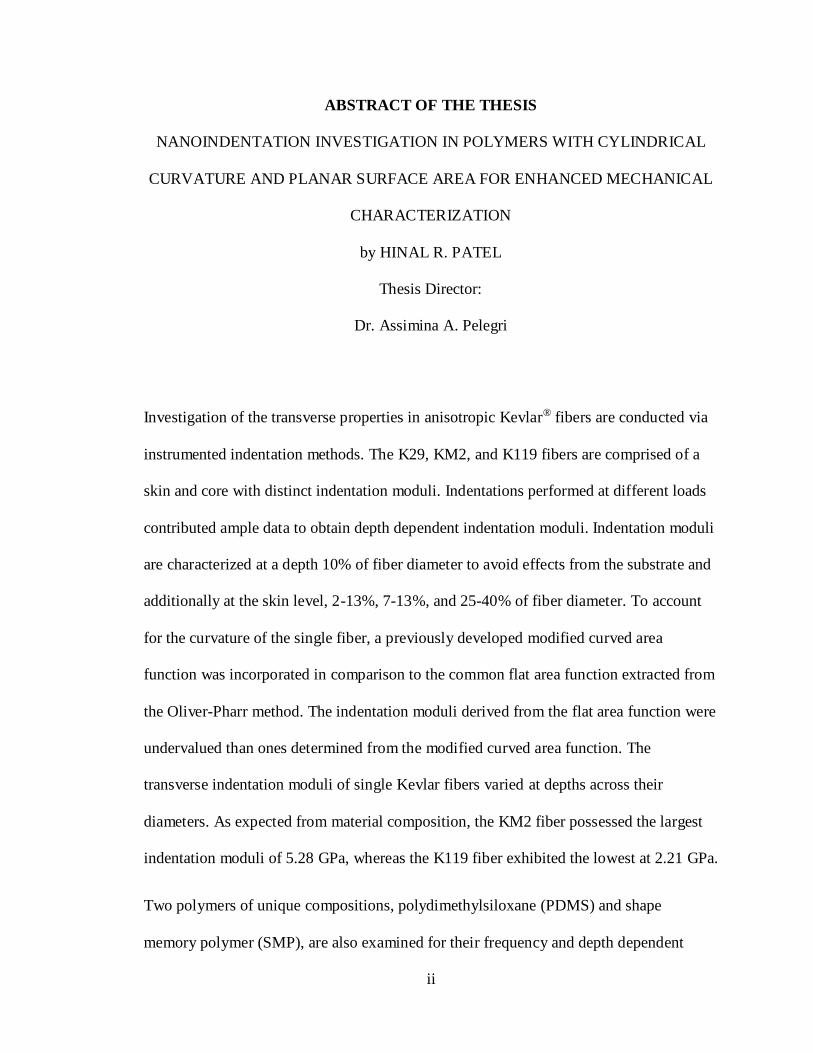
Investigation of the transverse properties in anisotropic Kevlar® fibers are conducted via
instrumented indentation methods. The K29, KM2, and K119 fibers are comprised of a
skin and core with distinct indentation moduli. Indentations performed at different loads
contributed ample data to obtain depth dependent indentation moduli. Indentation moduli
are characterized at a depth 10% of fiber diameter to avoid effects from the substrate and
additionally at the skin level, 2-13%, 7-13%, and 25-40% of fiber diameter. To account
for the curvature of the single fiber, a previously developed modified curved area
function was incorporated in comparison to the common flat area function extracted from
the Oliver-Pharr method. The indentation moduli derived from the flat area function were
undervalued than ones determined from the modified curved area function. The
transverse indentation moduli of single Kevlar fibers varied at depths across their
diameters. As expected from material composition, the KM2 fiber possessed the largest
indentation moduli of 5.28 GPa, whereas the K119 fiber exhibited the lowest at 2.21 GPa.
Two polymers of unique compositions, polydimethylsiloxane (PDMS) and shape
memory polymer (SMP), are also examined for their frequency and depth dependent

iii
mechanical properties via single and multiple cycle loading. PDMS is a hydrophobic
elastomer and exhibits greater elasticity than the hydrophilic SMP, but similarities in
material response were distinguished. During single cycle nanoindentation, both planar
polymers exhibited smoother loading curves at the lowest frequency as opposed to the
higher frequencies. At 3mN load-controlled tests, PDMS and SMP had an average
indentation modulus value of 3.94 ± 0.06 MPa and 2.07 ± 0.08 GPa, respectively. Their
indentation moduli differed by a factor of 525, supporting the conclusion that PDMS is
physically softer than the SMP. As loads and maximum depths increased, the mechanical
properties decreased for both materials.
To study periodic response behavior in both polymers, the frequencies for multiple cycle
tests were varied at 1, 0.5, and 0.033 Hz for different cycles. During these small-scale
fatigue tests on PDMS, 5 and 50 cycle experiments demonstrated a linear trend with a
negative slope for indentation moduli, whereas 100 cycle experimental data conformed to
power law curves. Contrarily, all cycles and frequencies tested on SMP followed power
law curve fitting. As the frequencies decreased, the change in maximum depths increased
along with a further depreciation of indentation modulus for both materials. The multiple
cycle indentation tests confirmed the consistent trends identified in the single cycle
indentations. Overall, the two polymers experienced comparable trends in mechanical
properties despite their extensive disparity in chemical composition, indentation modulus,
and hardness.

iv
ACKNOWLEDGEMENTS
I would like to proclaim my sincere gratitude for my thesis advisor and role model, Dr.
Mina Pelegri, who has generously supported and granted me the opportunity to conduct
research with her since 2015 as an undergraduate student. Her words of encouragement
guided me throughout my research and motivated me to obtain my MS at Rutgers
University.
Additionally, I want to thank Dr. Pelegri’s research group, especially Max Tenorio and
Hermise Raju, for their assistance in nanoindentation whenever I needed it. I am grateful
for Professor Howon Lee’s research group permitting me to test and analyze their
polymer specimens in conjunction for my thesis paper. Special thanks to Chen Yang for
assisting with sample preparation and analysis feedback. I would also like to
acknowledge my thesis committee: Prof. Mina Pelegri, Prof. Howon Lee, and Prof. Rajiv
Malhotra, for their time during the defense.
Finally, I want to thank my family, especially my mother and father, for their continuous
emotional and financial support. I would not be able to continue my education without
their encouragement and appreciation. I am so thankful for their unconditional love and
support.

v
TABLE OF CONTENTS
ABSTRACT OF THE THESIS ....................................................................................... ii
ACKNOWLEDGEMENTS ............................................................................................ iv
LIST OF TABLES .......................................................................................................... vii
LIST OF FIGURES ......................................................................................................... ix
LIST OF ACRONYMS AND SYMBOLS ................................................................... xiv
Chapter 1 – INTRODUCTION ....................................................................................... 1
Chapter 2 – BACKGROUND .......................................................................................... 5
2.1 – Indentation Theory .............................................................................................. 5
2.2 – Indentation Theory for Polymers ..................................................................... 10
2.3 – Berkovich Tip ..................................................................................................... 13
2.4 – Area functions..................................................................................................... 14
Chapter 3 – EXPERIMENTAL SETUP ....................................................................... 16
3.1 - Specimen Preparation ........................................................................................ 16
3.2 – Single and Multiple Cycle Loading Experimental Setup ............................... 18
3.3 – Table of Experiments ......................................................................................... 21
Chapter 4 – RESULTS AND DISCUSSION ................................................................ 24
4.1 – Indentation Moduli at 10% Kevlar Fiber Diameter ....................................... 25
4.1.1 Kevlar K29 Fiber.............................................................................................. 27
4.1.2 Kevlar KM2 Fiber ............................................................................................ 30
4.1.3 Kevlar K119 Fiber............................................................................................ 32
4.2 – Indentation Moduli at Various Percentages of Fiber Diameter .................... 34
4.2.1 Kevlar K29 Fiber.............................................................................................. 36
vi
4.2.2 Kevlar KM2 Fiber ............................................................................................ 38
4.2.3 Kevlar K119 Fiber............................................................................................ 39
4.3 PDMS Experimental Results ................................................................................ 40
4.3.1 PDMS – Single Cycle Loading ........................................................................ 41
4.3.2 PDMS – Multiple Cycle Loading .................................................................... 44
4.4 SMP Experimental Results................................................................................... 60
4.4.1 SMP – Single Cycle Loading ........................................................................... 60
4.4.2 SMP – Multiple Cycle Loading ....................................................................... 66
Chapter 5 – CONCLUSION .......................................................................................... 81
APPENDICES ................................................................................................................. 83
Appendix A – Kevlar 29 Supplementary Graphs .................................................... 83
Appendix B – Kevlar KM2 Supplementary Graphs ................................................ 85
Appendix C – Kevlar K119 Supplementary Graphs ............................................... 87
Appendix D – PDMS Supplementary Graphs .......................................................... 89
Appendix E – SMP Supplementary Graphs ............................................................. 97
REFERENCES .............................................................................................................. 105
vii
LIST OF TABLES
Table 3.1: Experiments on specimens of significant curvature (Kevlar fibers). .............. 21
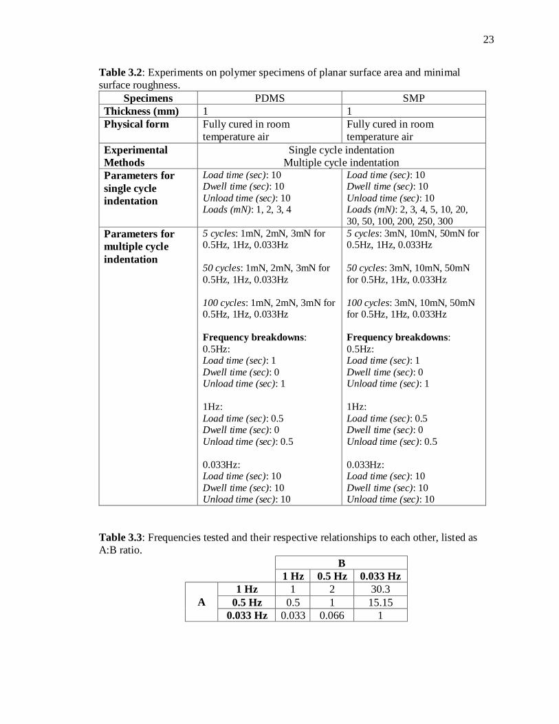
Table 3.2: Experiments on polymer specimens of planar surface area and minimal
surface roughness. ............................................................................................................. 23
Table 3.3: Frequencies tested and their respective relationships to each other, listed as
A:B ratio............................................................................................................................ 23
Table 4.1: The loads tested on three different types of fibers. The symbol (*) denotes the
load tested which reached 10% of fiber diameter. ............................................................ 26
Table 4.2: Average indentation moduli computed from both mCAF and FAF at 10% of
Kevlar fiber diameter. ....................................................................................................... 26
Table 4.3: Indentation modulus computed with mCAF at skin, 2-13%, 7-13%, and 25-
40% of fiber diameter for Kevlar fibers. ........................................................................... 35
Table 4.4: Indentation modulus computed with FAF at skin, 2-13%, 7-13%, and 25-40%
of fiber diameter for Kevlar fibers. ................................................................................... 35
Table 4.5: Two nanoindentation methods listed with the load-controlled tests on PDMS.
........................................................................................................................................... 40
Table 4.6: PDMS characterization of indentation modulus and hardness over a range of
depths through 1mm specimen thickness. ........................................................................ 42
Table 4.7: Multiple cycle indentation load-controlled tests for PDMS at frequencies of 1,
0.5, and 0.033Hz. Each frequency test was performed with 5, 50, and 100 cycles. Each
test had a corresponding maximum and minimum indentation modulus. ........................ 45
Table 4.8: Two nanoindentation methods listed with the load-controlled tests on SMP. 60

viii
Table 4.9: SMP characterization of indentation modulus and hardness over a range of
depths through 1mm specimen thickness. ........................................................................ 64
Table 4.10: Multiple cycle indentation load-controlled tests for SMP at frequencies of 1,
0.5, and 0.033Hz. Each frequency test was performed with 5, 50, and 100 cycles. Each
test had a corresponding maximum and minimum indentation modulus. ........................ 66
ix
LIST OF FIGURES
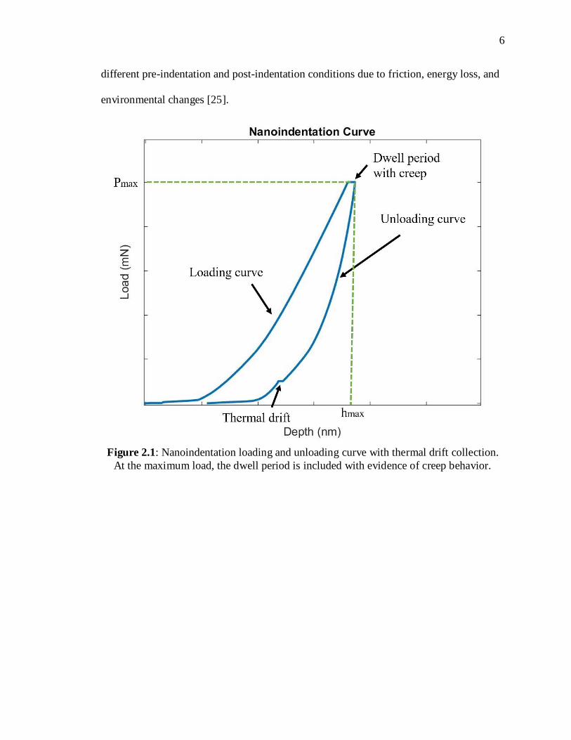
Figure 2.1: Nanoindentation loading and unloading curve with thermal drift collection.
At the maximum load, the dwell period is included with evidence of creep behavior. ...... 6
Figure 2.2: Stiffness is extrapolated from the slope of the unloading curve. The stiffness
is used in the calculation of the reduced modulus material property. ................................. 7
Figure 2.3: Specimen profile before, during, and after loading from the indenter tip. A
depression from the indenter tip is typically left after the maximum load is applied. ........ 8
Figure 2.4: Schematic of indentation marks from Berkovich indenter with (a) pile-up, (b)
no pile-up or sink-in, and (c) sink-in. The pile-up and sink-in effects can cause
inaccuracies in mechanical property calculations. ............................................................ 11
Figure 2.5: Multiple cycle loading hysteresis curve with five cycles. Each cycle has the
same frequency although the displacements between the cycles may vary...................... 12
Figure 2.6: The Berkovich indenter tip with a face half angle of 65.3°. The indenter tip is
made of diamond with a three-sided pyramidal geometry................................................ 13
Figure 2.7: Circled in red is an indent made by the Berkovich indenter. Its size is in the
same order of magnitude of the Kevlar fiber diameter; thus, incorporation of fiber
curvature is paramount to the accuracy of measurements. ............................................... 14
Figure 3.1: The single Kevlar fiber was carefully hang between two notches where the
adhesive was applied. In order for the steel washers to hang freely, pliers were utilized to
suspend the SEM puck stem on the edge of a table. ......................................................... 17
Figure 3.2: The pendulum components from the low load head in the Vantage. The
depth-sensing capacitor and electromagnetic coils provide precise control of the load and

x
depth. The balance weight is used for load calibration, which needs to be done whenever
the pendulum is removed from the low load head. ........................................................... 19
Figure 3.3: SMP mounted on Vantage in front of the Berkovich indenter. ..................... 20
Figure 4.1: Indentation moduli from the mCAF measured at indentation depth equal to
10% of the fiber diameter. ................................................................................................ 27
Figure 4.2: SEM picture of K29 fiber before treatment in denatured alcohol. The fiber
has a rough surface, which is clearly visible..................................................................... 28
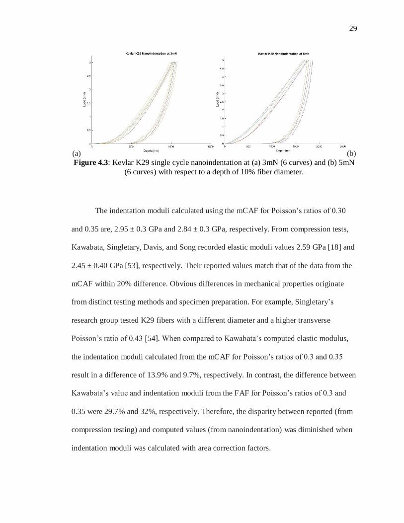
Figure 4.3: Kevlar K29 single cycle nanoindentation at (a) 3mN (6 curves) and (b) 5mN
(6 curves) with respect to a depth of 10% fiber diameter. ................................................ 29
Figure 4.4: SEM picture of KM2 fiber with clear distinction of a smoother surface than
the K29 fiber. .................................................................................................................... 31
Figure 4.5: Kevlar KM2 single cycle nanoindentation at 5mN (7 curves) with respect to a
depth of 10% fiber diameter. ............................................................................................ 32
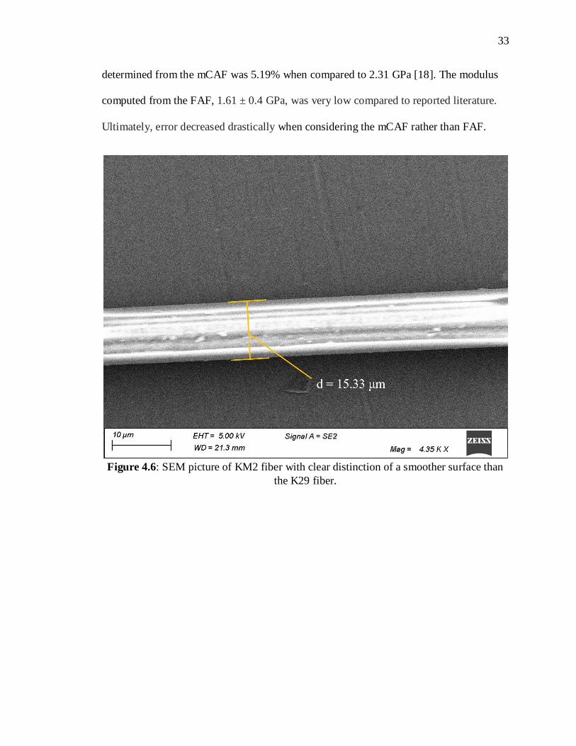
Figure 4.6: SEM picture of KM2 fiber with clear distinction of a smoother surface than
the K29 fiber. .................................................................................................................... 33
Figure 4.7: Kevlar K119 single cycle nanoindentation at 5mN (4 curves) with respect to
a depth of 10% fiber diameter. .......................................................................................... 34
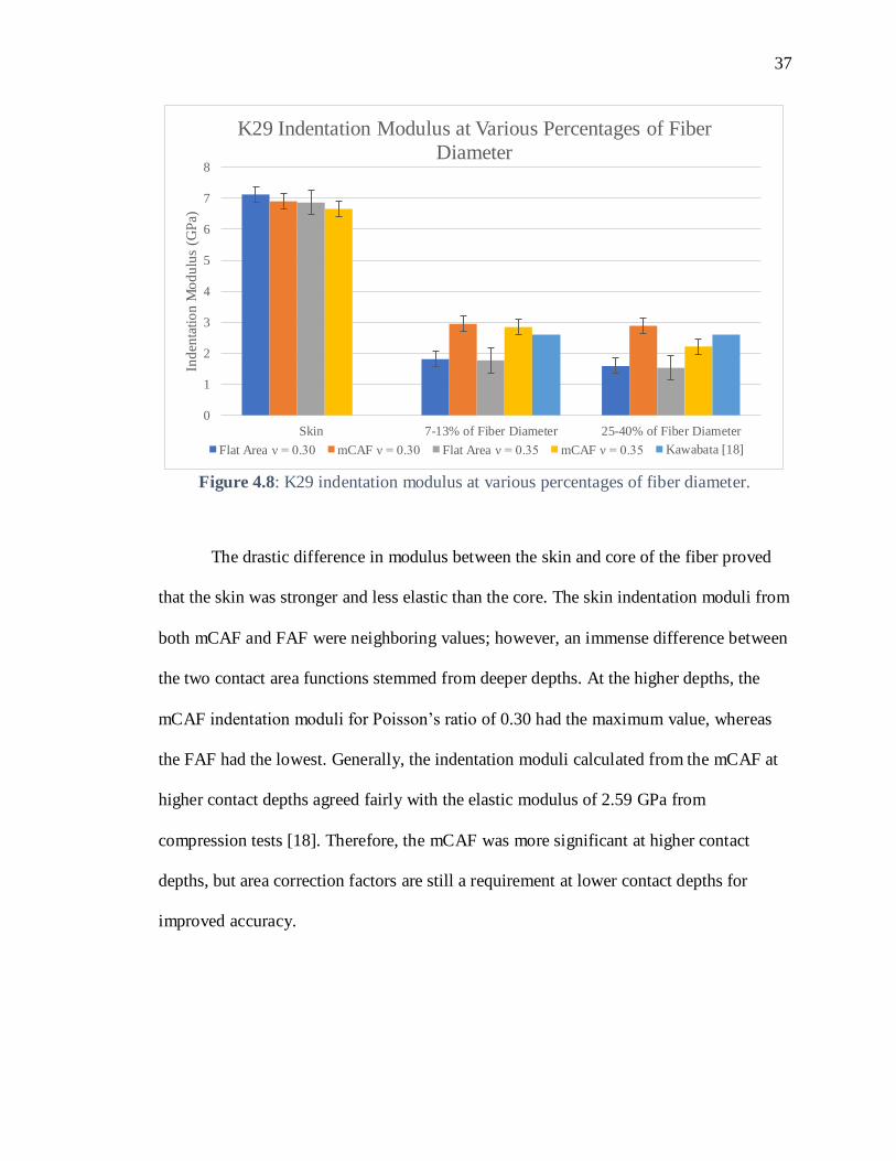
Figure 4.8: K29 indentation modulus at various percentages of fiber diameter. ............. 37
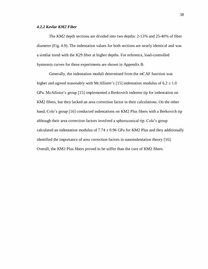
Figure 4.9: KM2 indentation modulus at various percentages of fiber diameter. ........... 39
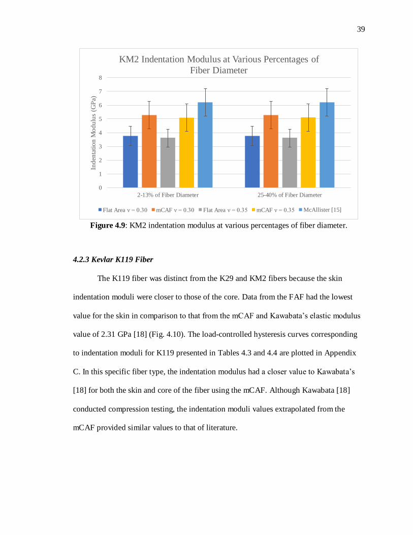
Figure 4.10: K119 indentation modulus at various percentages of fiber diameter. ......... 40
Figure 4.11: PDMS single cycle nanoindentation at (a) 1mN (8 curves), (b) 2mN (10
curves), (c) 3mN (10 curves), and (d) 4mN (10 curves). .................................................. 41
xi
Figure 4.12: Behavior of PDMS indentation modulus across a range of average
maximum depths. .............................................................................................................. 43
Figure 4.13: Behavior of PDMS hardness across a range of average maximum depths. 44
Figure 4.14: PDMS multiple cycle nanoindentation at 1mN and 5 cycles with varying
frequencies of (a) 1Hz (5 curves), (b) 0.5Hz (5 curves), (c) 0.033Hz (5 curves). ............ 46
Figure 4.15: PDMS indentation modulus graphs at 1mN with various frequencies at (a) 5
cycles, (b) 50 cycles, and (c) 100 cycles. .......................................................................... 48
Figure 4.16: PDMS indentation modulus graphs at 1mN with various cycles at (a) 1Hz,
(b) 0.5Hz, and (c) 0.033Hz. .............................................................................................. 49
Figure 4.17: PDMS hardness graphs at 1mN with various frequencies at (a) 5 cycles, (b)
50 cycles, and (c) 100 cycles. ........................................................................................... 50
Figure 4.18: PDMS hardness graphs at 1mN with various cycles at (a) 1Hz, (b) 0.5Hz,
and (c) 0.033Hz. ................................................................................................................ 51
Figure 4.19: PDMS indentation modulus graphs at 2mN with various frequencies at (a) 5
cycles, (b) 50 cycles, and (c) 100 cycles. .......................................................................... 52
Figure 4.20: PDMS indentation modulus graphs at 2mN with various cycles at (a) 1Hz,
(b) 0.5Hz, and (c) 0.033Hz. .............................................................................................. 53
Figure 4.21: PDMS hardness graphs at 2mN with various frequencies at (a) 5 cycles, (b)
50 cycles, and (c) 100 cycles. ........................................................................................... 54
Figure 4.22: PDMS hardness graphs at 2mN with various cycles at (a) 1Hz, (b) 0.5Hz,
and (c) 0.033Hz. ................................................................................................................ 55
Figure 4.23: PDMS indentation modulus graphs at 3mN with various frequencies at (a) 5
cycles, (b) 50 cycles, and (c) 100 cycles. .......................................................................... 56
xii
Figure 4.24: PDMS indentation modulus graphs at 3mN with various cycles at (a) 1Hz,
(b) 0.5Hz, and (c) 0.033Hz. .............................................................................................. 57
Figure 4.25: PDMS hardness graphs at 3mN with various frequencies at (a) 5 cycles, (b)
50 cycles, and (c) 100 cycles. ........................................................................................... 58
Figure 4.26: PDMS hardness graphs at 3mN with various cycles at (a) 1Hz, (b) 0.5Hz,
and (c) 0.033Hz. ................................................................................................................ 59
Figure 4.27: SMP single cycle nanoindentation at (a) 2mN (9 curves), (b) 3mN (8
curves), (c) 4mN (6 curves), and (d) 5mN (7 curves). ...................................................... 61
Figure 4.28: SMP single cycle nanoindentation at (a) 10mN (5 curves), (b) 20mN (10
curves), (c) 30mN (10 curves), and (d) 50mN (9 curves). ................................................ 62
Figure 4.29: SMP single cycle nanoindentation at (a) 100mN (6 curves), (b) 200mN (10
curves), (c) 250mN (10 curves), and (d) 300mN (8 curves). ............................................ 63
Figure 4.30: Behavior of SMP indentation modulus across a range of average maximum
depths. ............................................................................................................................... 65
Figure 4.31: Behavior of SMP hardness across a range of average maximum depths. ... 65
Figure 4.32: SMP multiple cycle nanoindentation at 3mN and 5 cycles with varying
frequencies of (a) 1Hz (7 curves), (b) 0.5Hz (7 curves), (c) 0.033Hz (7 curves). ............ 67
Figure 4.33: SMP indentation modulus graphs at 3mN with various frequencies at (a) 5
cycles, (b) 50 cycles, and (c) 100 cycles. .......................................................................... 69
Figure 4.34: SMP indentation modulus graphs at 3mN with various cycles at (a) 1Hz, (b)
0.5Hz, and (c) 0.033Hz. .................................................................................................... 70
Figure 4.35: SMP hardness graphs at 3mN with various frequencies at (a) 5 cycles, (b)
50 cycles, and (c) 100 cycles. ........................................................................................... 71

xiii
Figure 4.36: SMP hardness graphs at 3mN with various cycles at (a) 1Hz, (b) 0.5Hz, and
(c) 0.033Hz. ...................................................................................................................... 72
Figure 4.37: SMP indentation modulus graphs at 10mN with various frequencies at (a) 5
cycles, (b) 50 cycles, and (c) 100 cycles. .......................................................................... 73
Figure 4.38: SMP indentation modulus graphs at 10mN with various cycles at (a) 1Hz,
(b) 0.5Hz, and (c) 0.033Hz. .............................................................................................. 74
Figure 4.39: SMP hardness graphs at 10mN with various frequencies at (a) 5 cycles, (b)
50 cycles, and (c) 100 cycles. ........................................................................................... 75
Figure 4.40: SMP hardness graphs at 10mN with various cycles at (a) 1Hz, (b) 0.5Hz,
and (c) 0.033Hz. ................................................................................................................ 76
Figure 4.41: SMP indentation modulus graphs at 50mN with various frequencies at (a) 5
cycles, (b) 50 cycles, and (c) 100 cycles. .......................................................................... 77
Figure 4.42: SMP indentation modulus graphs at 50mN with various cycles at (a) 1Hz,
(b) 0.5Hz, and (c) 0.033Hz. .............................................................................................. 78
Figure 4.43: SMP hardness graphs at 50mN with various frequencies at (a) 5 cycles, (b)
50 cycles, and (c) 100 cycles. ........................................................................................... 79
Figure 4.44: SMP hardness graphs at 50mN with various frequencies at (a) 1Hz, (b)
0.5Hz, and (c) 0.033Hz. .................................................................................................... 80

xiv
LIST OF ACRONYMS AND SYMBOLS
PDMS Polydimethylsiloxane
SMP Shape memory polymer
BMA Benzyl methacrylate
BPA Bisphenol A ethoxylate dimethacrylate
FEM Finite element method
Pmax Maximum load
hmax Maximum depth
S Stiffness
P Load
h Depth
A Contact area
H Hardness
m Dimensionless constant for power law curve fitting
α Dimensionless constant for power law curve fitting
hf Final indentation depth
hc Contact depth
ε Geometric constant for the indenter tip
Er Reduced modulus
β Beta factor for the indenter tip
A(hc) Contact area as a function of contact depth
Es Indentation modulus of specimen
νs Poisson’s ratio of specimen

xv
νi Poisson’s ratio of indenter tip
Y Initial yield stress
E Elastic modulus
FAF Flat area function
d Average diameter
mCAF Modified curved area function
AmCAF(hc) Modified curved area function as a function of contact depth
DMA Dynamic mechanical analysis
1
Chapter 1 – INTRODUCTION
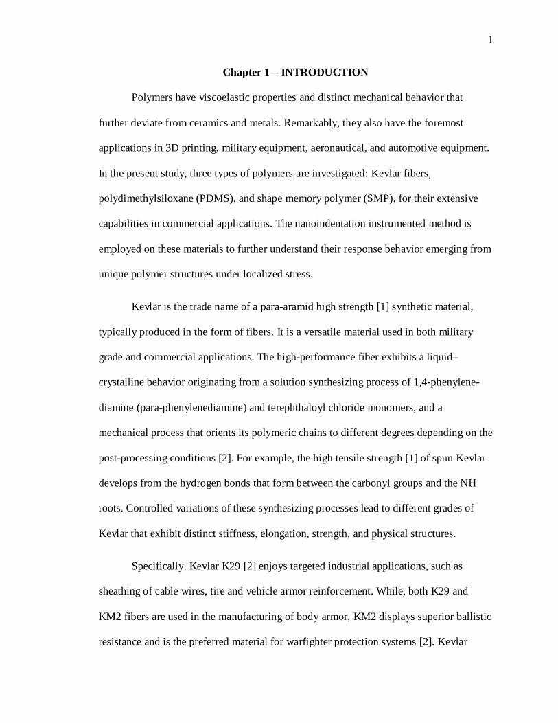
Polymers have viscoelastic properties and distinct mechanical behavior that
further deviate from ceramics and metals. Remarkably, they also have the foremost
applications in 3D printing, military equipment, aeronautical, and automotive equipment.
In the present study, three types of polymers are investigated: Kevlar fibers,
polydimethylsiloxane (PDMS), and shape memory polymer (SMP), for their extensive
capabilities in commercial applications. The nanoindentation instrumented method is
employed on these materials to further understand their response behavior emerging from
unique polymer structures under localized stress.
Kevlar is the trade name of a para-aramid high strength [1] synthetic material,
typically produced in the form of fibers. It is a versatile material used in both military
grade and commercial applications. The high-performance fiber exhibits a liquid–
crystalline behavior originating from a solution synthesizing process of 1,4-phenylene-
diamine (para-phenylenediamine) and terephthaloyl chloride monomers, and a
mechanical process that orients its polymeric chains to different degrees depending on the
post-processing conditions [2]. For example, the high tensile strength [1] of spun Kevlar
develops from the hydrogen bonds that form between the carbonyl groups and the NH
roots. Controlled variations of these synthesizing processes lead to different grades of
Kevlar that exhibit distinct stiffness, elongation, strength, and physical structures.
Specifically, Kevlar K29 [2] enjoys targeted industrial applications, such as
sheathing of cable wires, tire and vehicle armor reinforcement. While, both K29 and
KM2 fibers are used in the manufacturing of body armor, KM2 displays superior ballistic
resistance and is the preferred material for warfighter protection systems [2]. Kevlar

2
K119 is incorporated into clothing to protect against abrasions and heat. Fatigue resistant
K119 fibers elongate significantly and are a viable material for protective clothing [2].
Overall, the practical application of Kevlar, for both military and commercial uses,
confirms the need for continued research on the deformation of individual fibers as they
are exposed to concentrated forces.
As a well-known elastomer, PDMS, exhibits rubbery elasticity and is commonly
used in contact lenses [4] and biomechanical devices due to its nonbiodegradability [3].
This material’s unique viscoelastic properties are correlated with the combination of
silicone compounds and polymeric chains [3]. PDMS is incredibly soft, even the slightest
force causes major deformations. Conventionally, this material is a baseline comparison
with polymer behavior because of its chemical and mechanical stability and low loss
modulus [5].
The smart material, SMP, conforms temporarily upon external forces until an
external stimulus, such as heat, causes the polymer to restore its original form [6]. This
mechanical restoration response is a unique attribute of SMPs. Urinary catheters and
orthopedic braces require materials like SMPs that designate the medical device as
mendable and custom fit for a patient [7, 8]. Ge’s research group studied 4D printing
applications with SMPs in manufacturing of polymer grippers and springs [9]. These
mechanical tools adjust to a variety of sizes and prove crucial in systems that require soft
materials to maintain form. Yang et al. further investigated the viability of shock
absorbance on SMPs for aerospace structures and biomedical devices [10]. Evidently,
SMPs provide an extensive list of medical and commercial applications.
3
Experimental and computational techniques have been proposed to explore the
complex behavior and mechanical response of polymers. Compression and indentation
tests are few of the numerous methods employed to understand material behavior.
Indentation testing evaluates the indentation moduli of specimen at specified loads and
depths. Pressure from applied load is localized on the contact area between the specimen
and indenter tip. Meanwhile, compression testing relies on globally deforming the
specimen to find stress and strain relations. The procedure is generally performed with
two flat plates pushing together on both sides of the specimen to induce elastic
deformation. The stress is globalized on the surface area of the specimen that is in contact
with the plates. The specimen may yield causing plastic deformation and ultimately lead
to fracture in both testing methods if loads are increased. These methods offer valid
techniques for measuring mechanical properties of polymers and their unconventional
behavior.
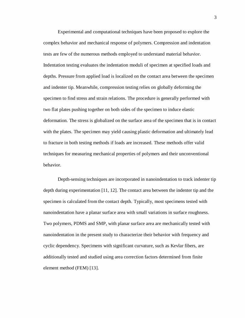
Depth-sensing techniques are incorporated in nanoindentation to track indenter tip
depth during experimentation [11, 12]. The contact area between the indenter tip and the
specimen is calculated from the contact depth. Typically, most specimens tested with
nanoindentation have a planar surface area with small variations in surface roughness.
Two polymers, PDMS and SMP, with planar surface area are mechanically tested with
nanoindentation in the present study to characterize their behavior with frequency and
cyclic dependency. Specimens with significant curvature, such as Kevlar fibers, are
additionally tested and studied using area correction factors determined from finite
element method (FEM) [13].
4
McAllister, Gillespie, VanLandingham, Cole, Strawhecker, Bencomo-Cisneros,
Tejeda-Ochoa, García-Estrada, Herrera-Ramírez, Hurtado-Macías, Martínez-Sánchez,
and Herrera-Ramírez have similarly tested Kevlar’s mechanical performance via
nanoindentation testing methods [14, 15, 16, 17]. However, their analysis lacked a proper
area correction function. Likewise, Kawabata, Wollbrett-Blitz, Joannès, Bruant, Le Clerc,
De La Osa, Bunsell, and Marcellan [18, 19] employed compression testing on single
Kevlar fibers to calculate their elastic modulus. Mechanical response, specifically for
Kevlar, from these two testing methods are compared with the findings from the newly
identified area correction factor. Although compression tests are a distinct method of
determining the elastic modulus of a material, they provide adequate comparisons to the
indentation modulus. The indentation modulus and elastic modulus are equivalent in most
materials where pile-up and sink-in are not present [20]. Caution must be taken when
comparing the same mechanical property measured from indentation and compression
testing because the specimens are distinctly compressed in each method.
Carillo’s research group analyzed the wet and fully cured states of PDMS via
nanoindentation testing [21]. Their research group additionally studied the different
variations between base to crosslinker ratios. The indentation moduli differences between
cracked and pristine PDMS elastomers was studied by Maji’s research group examined
with nanoindentation [22]. The present study of PDMS nanoindentation is compared to
these literature reports. Subsequently, the mechanical behavior of PDMS is additionally
compared to the newly formulated SMP specimen as a baseline comparison for polymer
behavior. Although these two polymers have distinct differences in softness, their
comparison provides further insight in material strength and applications.
5
Chapter 2 – BACKGROUND
2.1 – Indentation Theory
Indentation measurements rely on an applied load and contact depth between the
tip and the specimen to determine hardness and indentation modulus. This applied load
on the specimen results in elastic-plastic deformation that depends on the material
properties, load, and the depth. During the process of a single indent, the user inputs
either a maximum load or depth for the indenter tip to apply on a small specimen. Small
volume specimens are typically tested via nanoindentation at the sub-micron scale. The
indentations completed on thin films must provide that the indentation depth does not
surpass 10% of the specimen thickness to avoid the substrate effect [23]. The substrate
effect can influence the indentation modulus measurements and cause them to deviate
from their true values.
During the indentation test, the indenter tip applies a load on the specimen at a
single point and unloads after it reaches the maximum load. Each indent corresponds to a
loading and unloading curve (Fig. 2.1) and provides information of the maximum load,
Pmax, and the maximum depth, hmax. It also displays the dwell period, or the holding time,
when the indenter tip reaches the maximum load. During the dwell period, creep takes
place in the material and is physically represented by the increase of depth as the load
remains constant. A small holding time may lead to little or no creep depending on the
material [24]. Located on the unloading curve, the thermal drift correction exhibits creep
behavior and measures the change in thermal effects as the depth decreases and the load
is held constant. It is crucial to collect thermal drift data because the material may exhibit
6
different pre-indentation and post-indentation conditions due to friction, energy loss, and
environmental changes [25].
Figure 2.1: Nanoindentation loading and unloading curve with thermal drift collection.
At the maximum load, the dwell period is included with evidence of creep behavior.

7
Figure 2.2: Stiffness is extrapolated from the slope of the unloading curve. The stiffness
is used in the calculation of the reduced modulus material property.
The most common methods governing indentation theory are Oliver-Pharr [26] and
Doerner-Nix [27]. Regarding these methods, the slope of the unloading curve is equal to
the stiffness, S, of the specimen at the indentation location (Fig. 2.2). The formula for the
stiffness in terms of the load, P, and the indentation depth, h, is expressed as
𝑆 =𝑑𝑃
𝑑ℎ (1)

8
The hardness, H, is calculated with the maximum load and the contact area, A
from
𝐻 =𝑃𝑚𝑎𝑥
𝐴 (2)
The specimen is assumed to be completely flat and comparable to a semi-infinite plane in
both Oliver-Pharr [26] and Doerner-Nix [27] analysis. During an experiment, the indenter
tip depresses the specimen surface and an indent mark is formed (Fig. 2.3). Typically,
higher loads and indentation depths are correlated with larger contact areas and indent
sizes. Ultimately, indent size yielded from the localized plastic deformation process
depends on the maximum depth, load, and material properties.
Figure 2.3: Specimen profile before, during, and after loading from the indenter tip. A
depression from the indenter tip is typically left after the maximum load is applied.

9
The Oliver-Pharr method [26] relies on a power law function
𝑃 = 𝛼(ℎ − ℎ𝑓)𝑚
(3)
for characterization of the unloading curve in which m and α are dimensionless constants.
The final indentation depth, hf, is assumed to be zero only at elastic loads.
Depth-sensing techniques are necessary to calculate contact depth, hc, from
ℎ𝑐 = ℎ𝑚𝑎𝑥 − 𝜀𝑃𝑚𝑎𝑥
𝑆
(4)
where the geometric constant, ε, is unique to the indenter tip shape. The contact depth
refers to the deformation that occurs on the specimen’s surface during indentation (Fig
2.3). The indentation stiffness, S, is directly proportional to the material’s reduced
modulus, Er, and its relationship is given by
𝐸𝑟 =𝑆
2𝛽√
𝜋
𝐴(ℎ𝑐) (5)
This relationship was discovered from the extended Hertzian theory and nanoindentation
elastic field analysis [28]. Beta factor, β, is distinct for each indenter tip geometry and is
required to calculate the reduced modulus of the material. The contact area, A(hc), is
evaluated at the specific contact depth for that individual indent. Furthermore, reduced
modulus of the specimen is converted to the indentation modulus of the specimen, Es,
[29] from
1
𝐸𝑟=1 − 𝜈𝑠
2
𝐸𝑠+1 − 𝜈𝑖
2
𝐸𝑖 (6)
The Poisson’s ratios of the specimen, νs, and the indenter tip, νi, are necessary to convert
between the reduced and indentation moduli. The Poisson’s ratio for the Berkovich
diamond indenter tip is 0.07 and its elastic modulus, Ei, is 1141 GPa [30].
10
2.2 – Indentation Theory for Polymers
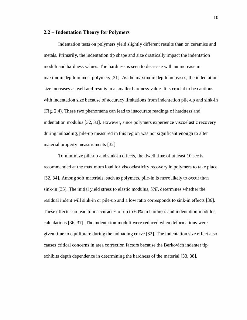
Indentation tests on polymers yield slightly different results than on ceramics and
metals. Primarily, the indentation tip shape and size drastically impact the indentation
moduli and hardness values. The hardness is seen to decrease with an increase in
maximum depth in most polymers [31]. As the maximum depth increases, the indentation
size increases as well and results in a smaller hardness value. It is crucial to be cautious
with indentation size because of accuracy limitations from indentation pile-up and sink-in
(Fig. 2.4). These two phenomena can lead to inaccurate readings of hardness and
indentation modulus [32, 33]. However, since polymers experience viscoelastic recovery
during unloading, pile-up measured in this region was not significant enough to alter
material property measurements [32].
To minimize pile-up and sink-in effects, the dwell time of at least 10 sec is
recommended at the maximum load for viscoelasticity recovery in polymers to take place
[32, 34]. Among soft materials, such as polymers, pile-in is more likely to occur than
sink-in [35]. The initial yield stress to elastic modulus, Y/E, determines whether the
residual indent will sink-in or pile-up and a low ratio corresponds to sink-in effects [36].
These effects can lead to inaccuracies of up to 60% in hardness and indentation modulus
calculations [36, 37]. The indentation moduli were reduced when deformations were
given time to equilibrate during the unloading curve [32]. The indentation size effect also
causes critical concerns in area correction factors because the Berkovich indenter tip
exhibits depth dependence in determining the hardness of the material [33, 38].

11
Figure 2.4: Schematic of indentation marks from Berkovich indenter with (a) pile-up, (b)
no pile-up or sink-in, and (c) sink-in. The pile-up and sink-in effects can cause
inaccuracies in mechanical property calculations.
Typically, the indentation modulus for most materials is acknowledged to be
identical to the elastic modulus [39]. Elastic modulus and indentation modulus are
comparable, but effects of pile-up and sink-in must be carefully examined when referring
to the indentation modulus as the elastic modulus. It is preferred to consider differences
in moduli based on testing methods that include globally and locally compressing the
specimens. Compression and tensile testing globally test the specimen, whereas
indentation tests locally compresses the specimen. Pile-up can cause an overestimation of
indentation modulus but permitting for an adequate dwell time for a steady strain rate can
mitigate the problem [32, 34, 39]. Specifically, the indentation modulus of polymers is a
combination of the elastic and the viscous response of the material [40]. Even though
time-dependent viscoelastic recoveries of the polymer are not isolated in nanoindentation,
the indentation modulus unequivocally bestows practical information about the quasi
static material behavior response.
12
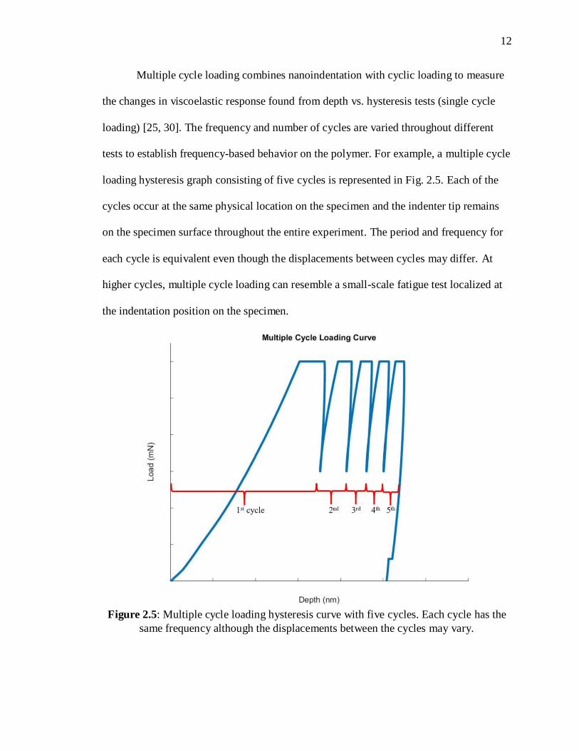
Multiple cycle loading combines nanoindentation with cyclic loading to measure
the changes in viscoelastic response found from depth vs. hysteresis tests (single cycle
loading) [25, 30]. The frequency and number of cycles are varied throughout different
tests to establish frequency-based behavior on the polymer. For example, a multiple cycle
loading hysteresis graph consisting of five cycles is represented in Fig. 2.5. Each of the
cycles occur at the same physical location on the specimen and the indenter tip remains
on the specimen surface throughout the entire experiment. The period and frequency for
each cycle is equivalent even though the displacements between cycles may differ. At
higher cycles, multiple cycle loading can resemble a small-scale fatigue test localized at
the indentation position on the specimen.
Figure 2.5: Multiple cycle loading hysteresis curve with five cycles. Each cycle has the
same frequency although the displacements between the cycles may vary.
13
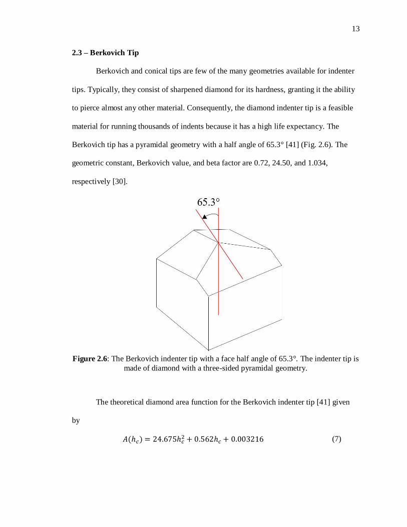
2.3 – Berkovich Tip
Berkovich and conical tips are few of the many geometries available for indenter
tips. Typically, they consist of sharpened diamond for its hardness, granting it the ability
to pierce almost any other material. Consequently, the diamond indenter tip is a feasible
material for running thousands of indents because it has a high life expectancy. The
Berkovich tip has a pyramidal geometry with a half angle of 65.3° [41] (Fig. 2.6). The
geometric constant, Berkovich value, and beta factor are 0.72, 24.50, and 1.034,
respectively [30].
Figure 2.6: The Berkovich indenter tip with a face half angle of 65.3°. The indenter tip is
made of diamond with a three-sided pyramidal geometry.
The theoretical diamond area function for the Berkovich indenter tip [41] given
by
𝐴(ℎ𝑐) = 24.675ℎ𝑐2 + 0.562ℎ𝑐 + 0.003216 (7)

14
is necessary for determining area contact between the specimen and tip. Commonly, the
diamond area function is calibrated on quartz since Berkovich tips may vary in shapes
after a plethora of indents.
The radius of the indenter tip is comparable to both the nanometer scale and
Kevlar fiber diameter of micrometers [20, 39]. For comparison, a Berkovich indent on a
SEM stub next to a single Kevlar K29 fiber is displayed in Fig. 2.7. The indent size is
commensurable to the fiber diameter; therefore, indicating the importance of an area
correction factor between the fiber’s significant curvature and the indenter tip.
Figure 2.7: Circled in red is an indent made by the Berkovich indenter. Its size is in the
same order of magnitude of the Kevlar fiber diameter; thus, incorporation of fiber
curvature is paramount to the accuracy of measurements.
2.4 – Area functions
Accuracy in applying proper area functions is crucial to calculate the correct
contact area and reduced modulus. The contact area depends on the contact depth,

15
constants relative to the geometry of the indenter tip, and the specimen surface
roughness. Area correction is necessary for specimens, such as a single Kevlar fiber, with
significant curvature and diameter comparable to the indent size (Fig. 2.7).
The standard Oliver-Pharr analysis considers the specimen to be a perfect semi-
infinite plane and is applicable for planar specimens with small changes in surface
roughness [26]. In cases where the specimen contains significant curvature, a modified
user-defined area function must be determined to correctly calculate mechanical
properties of the specimen.
The area function corresponding to the standard Oliver-Pharr method uses Eq. (7)
and a fitted diamond area polynomial function (calibrated with quartz). The combined
function is referred to as the flat area function (FAF) because it assumes that the surface
geometry of the specimen is a semi-infinite plane. The order of the polynomial depends
on the depth; if the maximum depth is less than 1,000nm, the order used is five,
otherwise the order used is two. The FAF calculates the correct contact area for the SMP
and PMDS (planar) specimens, but not the Kevlar samples due to significant curvature.
The modified user-defined function was developed with finite element analysis by
considering the curvature of the fiber and Berkovich tip shape to establish the modified
curved area function (mCAF) [13] as
𝐴𝑚𝐶𝐴𝐹(ℎ𝑐) = [2.791 ln(𝑑)− 1.9447]ℎ𝑐2 + [1.547 ln(𝑑) + 1.9323]103ℎ𝑐 (8)
where the mCAF depends on the average diameter, d. Therefore, each type of Kevlar
fiber tested will have its own unique mCAF coefficients. The indentation moduli,
specifically for Kevlar fibers, found from both the mCAF and FAF are compared to
literature to provide insight on the significance of modified contact area.

16
Chapter 3 – EXPERIMENTAL SETUP
3.1 - Specimen Preparation
Three different types of specimens were prepared: single Kevlar fibers (K29,
KM2, and K119), polydimethylsiloxane (PDMS), and shape memory polymer (SMP). All
single Kevlar fiber specimens were primed in the same methods, except Kevlar K29.
Prior to mounting, the K29 fiber was pretreated in denatured alcohol for 12 hours to
smoothen its uneven surface roughness. PDMS and SMP specimens were fabricated in
the laboratory, while the Kevlar fibers were obtained directly from DuPont.
Preparing the Kevlar fiber specimens required the SEM stub to be prepped before
the fibers were attached. A hand file was used to create two notches on the SEM stub
which were located 180° apart from each other. The SEM stub was roughly sanded using
a metallographic manual wheel polisher. After the SEM stub surface was leveled, the
SEM stub was attached to a hand drill to be polished on 1000, 1500, 2000, and 2500 grit
sandpaper. Sanding pads with higher grit of 3200, 3600, 4000, 6000, and 12000 were
used for fine sanding. To provide a smooth surface for the fiber to lay, the SEM stub was
finished with polishing compound and a Dremel.
Each type of Kevlar fiber yarn (K29, KM2, and K119) was cut to five inches in
length and a single fiber was diligently extracted using tweezers. Each ends of the single
fiber were adhered to two 1.1g steel washers with Loctite 495 Super Bond Instant
Adhesive glue. Approximately after 24 hours, the fiber was placed between the notches
on the SEM stub with the two washers suspended off each side. The same adhesive was
used to glue the fiber to the SEM stub near the notches (Fig. 3.1). The washers were

17
clipped off when the adhesive dried in 24 hours. This method was adopted from the
nanoindentation Kevlar studies by Turla, Raju, and Pelegri [13, 42].
Figure 3.1: The single Kevlar fiber was carefully hung between two notches where the
adhesive was applied. In order for the steel washers to hang freely, pliers were utilized to
suspend the SEM puck stem on the edge of a table.
The polydimethylsiloxane (PDMS, (C2H6OSi)n) specimen was cured with a
Sylgard 184 silicone elastomer base and silicone elastomer crosslinker (10:1 weight ratio)
[43]. The mixed polymer was degassed for 30 minutes to remove air bubbles trapped during
mixing. Then the mixture was injected between two glass microscope slides separated by
1mm spacers and was heated at 70˚C for 5 hours. The cured elastomer was carefully
extracted from the glass slides using a razor blade and cut into a square with a length of
1cm. It was mounted on a polished SEM stub with Loctite 495 Super Bond Instant
Adhesive glue and left to dry for 12 hours.

18
The shape memory polymer (SMP) was prepared with a 4:1 (weight ratio) mixture
of Benzyl-methacrylate (BMA, C11H12O2) and Bisphenol A ethoxylate dimethacrylate
(BPA, [H2C=C(CH3)CO2(CH2CH2O)nC6H4-4-]2C(CH3)2). The SMP precursor resin was
injected between two glass slides separated by 1mm spacers. The solution was set to cure
in 365 nm UV oven for 20 minutes, similarly done by Safranski and Gall [44]. The glass
slides were removed using a razor blade and cut to an identical size as the PDMS specimens
to be mounted on a SEM stub with the same adhesive.
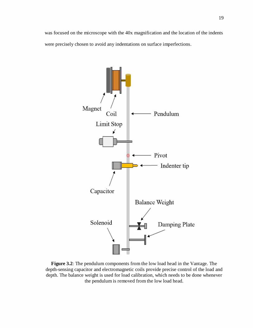
3.2 – Single and Multiple Cycle Loading Experimental Setup
The Micro Materials NanoTest Vantage was operated to investigate the
mechanical properties of the polymer specimens via nanoindentation. The Vantage
contains three main components: a microscope (with lenses of 5x, 10x, 20x, and 40x
magnification), sample stage, and low load head (contains the pendulum and indenter
tip). A depth-sensing capacitor near the indenter tip measures the indentation depth and
the load is applied using an electromagnetic force from the magnet and coils (Fig. 3.2).
The load limits for the Vantage range from 0.5mN to 500mN and the maximum available
depth is around 20,000nm.
The environmental testing chamber was held at a constant temperature of 28°C
with 20% humidity and the Berkovich diamond indenter tip was fitted in the indenter
shaft for all indentation tests. The focal plane and cross hair calibrations were performed
for nanoindentation accuracy. Before each experiment, a pendulum balance test was
conducted to ensure the pendulum had a full-range of motion. Before data collection, the
specimen on the SEM stub was mounted to the Vantage’s sample stage. The specimen
19
was focused on the microscope with the 40x magnification and the location of the indents
were precisely chosen to avoid any indentations on surface imperfections.
Figure 3.2: The pendulum components from the low load head in the Vantage. The
depth-sensing capacitor and electromagnetic coils provide precise control of the load and
depth. The balance weight is used for load calibration, which needs to be done whenever
the pendulum is removed from the low load head.
20
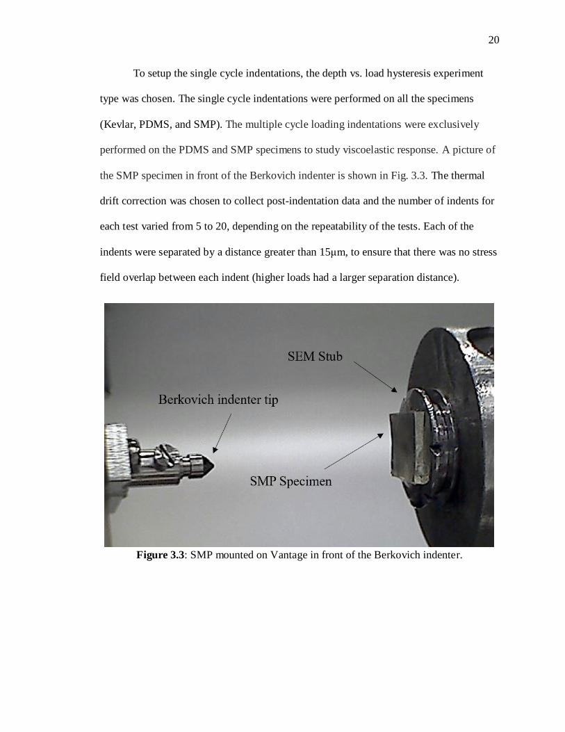
To setup the single cycle indentations, the depth vs. load hysteresis experiment
type was chosen. The single cycle indentations were performed on all the specimens
(Kevlar, PDMS, and SMP). The multiple cycle loading indentations were exclusively
performed on the PDMS and SMP specimens to study viscoelastic response. A picture of
the SMP specimen in front of the Berkovich indenter is shown in Fig. 3.3. The thermal
drift correction was chosen to collect post-indentation data and the number of indents for
each test varied from 5 to 20, depending on the repeatability of the tests. Each of the
indents were separated by a distance greater than 15μm, to ensure that there was no stress
field overlap between each indent (higher loads had a larger separation distance).
Figure 3.3: SMP mounted on Vantage in front of the Berkovich indenter.

21
3.3 – Table of Experiments
Single cycle loading was the only method tested on the Kevlar fibers to study the
variation of indentation modulus along the fiber diameter (Table 3.1). The parameters
used for each single cycle loading test included loading and unloading periods of 50 sec.
The extended loading and unloading times encouraged adjustments within fiber
dislocations to prevent slipping. The dwell time at maximum load and thermal drift
correction were 10 sec and 30 sec, respectively for all fibers. Kevlar K29 fibers were
tested at the following loads: 1mN through 3mN (increments of 1mN) and 5mN through
40mN (increments of 5mN). The KM2 fiber was tested at the same loads at the K29 fiber
excluding any loads greater than 25mN. Finally, loads ranging from 3mN through 40mN
were tested on the K119 fibers. Caution was taken with loads exceeding 50mN to prevent
breaking the fiber. The reduced modulus was calculated with the mCAF for cylindrical
area correction.
Table 3.1: Experiments on specimens of significant curvature (Kevlar fibers).
Specimens K29 KM2 K119
Diameter (μm) 14.6 12 15.33
Physical form Single fiber extracted
from yarn and treated
in denatured alcohol
Single fiber extracted from yarn
Experimental
Methods
Single cycle indentation
Parameters for
single cycle
indentation
Load time (sec): 50
Dwell period (sec): 10 Unload time (sec): 50
Loads (mN): 1, 2, 3, 5, 10, 15, 20, 25, 30, 35,
40
Load time (sec): 50
Dwell period (sec): 10
Unload time (sec): 50
Loads (mN): 1, 2, 3, 5, 10, 15, 20, 25
Load time (sec): 50
Dwell period (sec): 10
Unload time (sec): 50 Loads (mN): 3, 5, 10,
20, 25, 30, 35, 40
Caution Loads exceeding over 50mN may cause the fiber to break
Area correction is needed for all fibers in analysis

22
The experimental methods employed on specimens of planar surface geometry
were single and multiple cycle loading to study the significance of frequency dependence
(Table 3.2). The loading, unloading, and dwell times during the single cycle loading tests
were 10 sec to prevent ‘nosing’ in the hysteresis graphs [34]. These parameters resulted
in smoother unloading curves because the viscoelastic effects developed within that time
interval. Lower loads from 1 to 4mN were tested on the PDMS because it was very soft.
Contrarily, the SMP specimens were tested at a larger range of loads from 2mN through
300mN because it was able to maintain its form at higher loads.
Multiple cycle loading on the planar specimens were necessary to determine the
changes in viscoelastic response found in the hardness and indentation modulus values
[25]. During the multiple cycle indentation tests, the frequency ranges were varied at 1,
0.5, and 0.033Hz to examine the influence of frequency on the polymer specimens.
During 0.5Hz tests, the loading and unloading portions ran for 2 sec each with no hold
time at maximum load. Similarly, the 1Hz tests consisted of a loading and unloading time
of 0.5 sec each and no dwell period. Finally, the 0.033Hz tests carried out loading,
unloading, and hold time for 10 sec each. The comparison between frequencies for ease
are provided in Table 3.3, where the frequencies in column A are compared to those from
row B (A:B ratio). The cycles tested were 5, 50, and 100 for both specimens to study
cyclic dependency on polymers. The loads tested on PDMS with multiple cycle loading
were 1, 2, and 3mN, while SMP specimens were tested with 3, 10, and 50mN loads.
23
Table 3.2: Experiments on polymer specimens of planar surface area and minimal
surface roughness.
Specimens PDMS SMP
Thickness (mm) 1 1
Physical form Fully cured in room
temperature air
Fully cured in room
temperature air
Experimental
Methods
Single cycle indentation
Multiple cycle indentation
Parameters for
single cycle
indentation
Load time (sec): 10 Dwell time (sec): 10
Unload time (sec): 10 Loads (mN): 1, 2, 3, 4
Load time (sec): 10 Dwell time (sec): 10
Unload time (sec): 10 Loads (mN): 2, 3, 4, 5, 10, 20,
30, 50, 100, 200, 250, 300
Parameters for
multiple cycle
indentation
5 cycles: 1mN, 2mN, 3mN for 0.5Hz, 1Hz, 0.033Hz
50 cycles: 1mN, 2mN, 3mN for
0.5Hz, 1Hz, 0.033Hz
100 cycles: 1mN, 2mN, 3mN for 0.5Hz, 1Hz, 0.033Hz
Frequency breakdowns:
0.5Hz: Load time (sec): 1
Dwell time (sec): 0 Unload time (sec): 1
1Hz:
Load time (sec): 0.5 Dwell time (sec): 0
Unload time (sec): 0.5
0.033Hz: Load time (sec): 10
Dwell time (sec): 10 Unload time (sec): 10
5 cycles: 3mN, 10mN, 50mN for 0.5Hz, 1Hz, 0.033Hz
50 cycles: 3mN, 10mN, 50mN
for 0.5Hz, 1Hz, 0.033Hz
100 cycles: 3mN, 10mN, 50mN for 0.5Hz, 1Hz, 0.033Hz
Frequency breakdowns:
0.5Hz: Load time (sec): 1
Dwell time (sec): 0 Unload time (sec): 1
1Hz:
Load time (sec): 0.5 Dwell time (sec): 0
Unload time (sec): 0.5
0.033Hz: Load time (sec): 10
Dwell time (sec): 10 Unload time (sec): 10
Table 3.3: Frequencies tested and their respective relationships to each other, listed as
A:B ratio.
B
1 Hz 0.5 Hz 0.033 Hz
A
1 Hz 1 2 30.3
0.5 Hz 0.5 1 15.15
0.033 Hz 0.033 0.066 1

24
Chapter 4 – RESULTS AND DISCUSSION
For completeness of fiber characterization, the Kevlar single fibers are reported at
10% and up to 40% of the single fiber diameter in the present study. The fiber is treated
as a thin film because surface roughness is not comparable to the magnitude of its
diameter [15, 45, 46] and 0.1 ratio (depth to fiber diameter) rule was the basis for
assessing indentation moduli, originating from the substrate effect [45, 46]. Indentation
moduli corresponding to depths greater than 10% of fiber diameter were included in the
analysis, but the reliability of these results were taken with caution.
Two different area functions defined for fiber characterization, flat area function
(FAF) and modified curved area function (mCAF), were applied to compute the Kevlar
fiber indentation moduli. Error comparison was the sole purpose of tabulating the fiber
moduli yielded from the FAF. The polydimethylsiloxane (PDMS) and shape memory
polymer (SMP) planar specimens solely required the FAF for calculating indentation
moduli because they were relatively flat specimens with miniscule changes in surface
roughness.
Literature results from compression tests were compared to those of indentation
tests in the present study, but data was loosely considered because of differences in
methodology [20, 39, 47]. Studies indicating moduli results from indentation were also
examined for differences in material type, specimen preparation, and analysis. For
instance, some literature reports did not include area correction factors for their
indentation analysis of fibers [15]. Small discrepancies may arise between data with
variations in testing methods and analysis, hence they must be acknowledged as
approximations.
25
The transverse Poisson’s ratio for Kevlar fibers that did not have reported values
in literature were closely assessed based on bond composition. The estimation of this
ratio in anisotropic fibers is derived from the transverse angles formed between bonds
and crystalline geometry. Cheng, Chen, Weerasooriya, Muhammed, and Ismaeel reported
the transverse Poisson’s ratio of 0.35 for Kevlar KM2 [48] and K29 [49]. In respect to
their crystalline geometry, it is commonly estimated that both KM2 and K29 have a
Poisson’s ratio of 0.30 and K119 embodies a lower ratio of 0.27 [50]. Both ratios for
KM2 and K29 fibers are included for analysis to determine the importance of accuracy in
Poisson’s ratio. Conceptually, the requirement of exact Poisson’s ratios for Eq. (6)
proved to be insignificant in FEM analysis [13]. Similar trends with Poisson’s ratio
insignificance were observed in compression tests on single monofilament fibers [51, 52].
4.1 – Indentation Moduli at 10% Kevlar Fiber Diameter
Single cycle loading indentation method was performed on Kevlar fibers at
varying loads (Table 4.1). The asterisk (*) in Table 4.1 indicates that the corresponding
load-controlled test achieved a maximum depth neighboring 10% of fiber diameter. The
indentation tests designated with asterisks in Table 4.1 are separately examined for each
fiber at 10% diameter, while the rest of the loads are discussed from skin depth to 40% of
fiber diameter.

26
Table 4.1: The loads tested on three different types of fibers. The symbol (*) denotes the
load tested which reached 10% of fiber diameter.
Loads (mN) K29 KM2 K119
1 X X
2 X X
3 X* X X
5 X* X* X*
10 X X X
15 X X
20 X X X
25 X X X
30 X X
35 X X
40 X X
The two Poisson’s ratios of 0.30 and 0.35 (for KM2 and K29) are tabulated with
their corresponding indentation moduli computed from the mCAF and FAF in Table 4.2.
It was a common trend of 5mN load reaching a depth around 10% of fiber diameter
across all types of Kevlar tested, except 3mN was an additional load for K29. The
indentation moduli values analyzed from the FAF strayed further away from literature
values presented in Table 4.2. Rather, moduli computed with the mCAF were closer in
respect to reported literature and also larger in value than the ones calculated with the
FAF.
Table 4.2: Average indentation moduli computed from both mCAF and FAF at 10% of
Kevlar fiber diameter.
Fiber Fiber
Diameter
(μm)
Poisson’s
Ratio, ν
Es from
mCAF
(GPa)
Es from
FAF(GPa)
Literature
Modulus (GPa)
KM2 12 0.30 [50] 5.10 ± 0.4 3.34 ± 0.3 6.2 ± 1.0 [15]
0.35 [48,49] 4.91 ± 0.4 3.22 ± 0.3
K29 14.6 0.30 [50] 2.95 ± 0.3 1.82 ± 0.3 2.59 [18]
0.35 [48,49] 2.84 ± 0.3 1.76 ± 0.3
K119 15.33 0.27 [50] 2.43 ± 0.4 1.61 ± 0.4 2.31 [18]
27
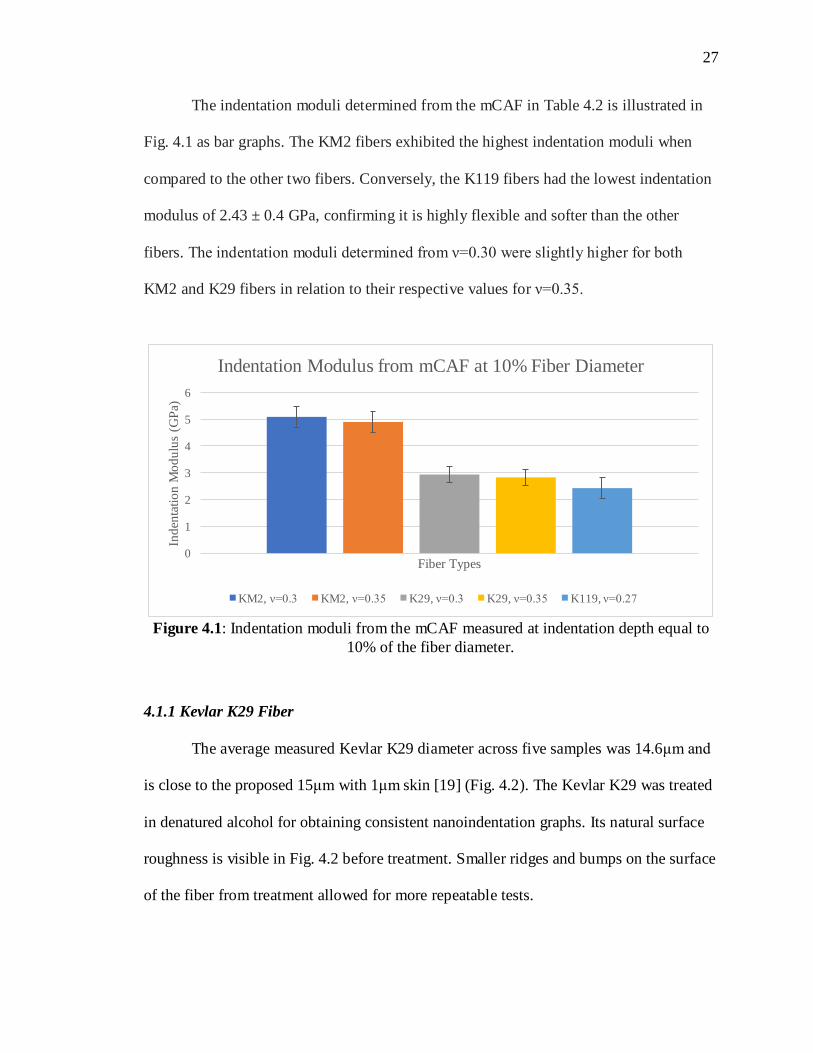
The indentation moduli determined from the mCAF in Table 4.2 is illustrated in
Fig. 4.1 as bar graphs. The KM2 fibers exhibited the highest indentation moduli when
compared to the other two fibers. Conversely, the K119 fibers had the lowest indentation
modulus of 2.43 ± 0.4 GPa, confirming it is highly flexible and softer than the other
fibers. The indentation moduli determined from ν=0.30 were slightly higher for both
KM2 and K29 fibers in relation to their respective values for ν=0.35.
Figure 4.1: Indentation moduli from the mCAF measured at indentation depth equal to
10% of the fiber diameter.
4.1.1 Kevlar K29 Fiber
The average measured Kevlar K29 diameter across five samples was 14.6μm and
is close to the proposed 15μm with 1μm skin [19] (Fig. 4.2). The Kevlar K29 was treated
in denatured alcohol for obtaining consistent nanoindentation graphs. Its natural surface
roughness is visible in Fig. 4.2 before treatment. Smaller ridges and bumps on the surface
of the fiber from treatment allowed for more repeatable tests.
0
1
2
3
4
5
6
Ind
enta
tio
n M
od
ulu
s (G
Pa)
Fiber Types
Indentation Modulus from mCAF at 10% Fiber Diameter
KM2, ν=0.3 KM2, ν=0.35 K29, ν=0.3 K29, ν=0.35 K119, ν=0.27

28
Figure 4.2: SEM picture of K29 fiber before treatment in denatured alcohol. The fiber
has a rough surface, which is clearly visible.
At 3 and 5mN loads, 20 indents were performed under load-controlled conditions
on single K29 fibers, out of which, the six most representative are presented in Fig. 4.3.
The indentation depth for 3mN was slightly below 10% fiber diameter, while the depth at
5mN was just above 10% fiber diameter. Evidently, both sets of data are incorporated in
the indentation modulus of K29 at 10% of the fiber diameter in Table 4.2.
29
(a) (b)
Figure 4.3: Kevlar K29 single cycle nanoindentation at (a) 3mN (6 curves) and (b) 5mN
(6 curves) with respect to a depth of 10% fiber diameter.
The indentation moduli calculated using the mCAF for Poisson’s ratios of 0.30
and 0.35 are, 2.95 ± 0.3 GPa and 2.84 ± 0.3 GPa, respectively. From compression tests,
Kawabata, Singletary, Davis, and Song recorded elastic moduli values 2.59 GPa [18] and
2.45 ± 0.40 GPa [53], respectively. Their reported values match that of the data from the
mCAF within 20% difference. Obvious differences in mechanical properties originate
from distinct testing methods and specimen preparation. For example, Singletary’s
research group tested K29 fibers with a different diameter and a higher transverse
Poisson’s ratio of 0.43 [54]. When compared to Kawabata’s computed elastic modulus,
the indentation moduli calculated from the mCAF for Poisson’s ratios of 0.3 and 0.35
result in a difference of 13.9% and 9.7%, respectively. In contrast, the difference between
Kawabata’s value and indentation moduli from the FAF for Poisson’s ratios of 0.3 and
0.35 were 29.7% and 32%, respectively. Therefore, the disparity between reported (from
compression testing) and computed values (from nanoindentation) was diminished when
indentation moduli was calculated with area correction factors.

30
4.1.2 Kevlar KM2 Fiber
The measured average diameter of KM2 fibers across four samples was 12μm
with a skin thickness of 200 nm [14, 42]. The KM2 fiber, shown in Fig. 4.4, was
generally smoother than the K29 fiber. McAllister’s research group concluded KM2’s
indentation modulus was 6.2 ± 1.0 GPa using a Berkovich tip without any area correction
factors [15]. Although their values largely diverged from FAF values reported in Table
4.2, the mCAF results displayed substantial compliance with their findings. The
calculated indentation modulus of KM2 Plus from Cole’s research group was 7.74 ± 0.96
GPa [16]. Although KM2 Plus was not a specimen examined in the present study, it was
clearly stiffer than the original KM2. Cole’s study additionally implemented a Berkovich
indenter, but their area correction analysis assumed the indenter to have a spheroconical
geometry [16]. The differences between the contact area of spheroconical and Berkovich
geometry are noticeably different arising from their distinct area functions [41]. Hence,
the mCAF accurately incorporates the Berkovich indenter’s pyramidal geometry for
modulus calculation.

31
Figure 4.4: SEM picture of KM2 fiber with clear distinction of a smoother surface than
the K29 fiber.
The indentation moduli for 10% KM2 fiber diameter in Table 4.2 originate from
the 5mN hysteresis curves (Fig 4.5). The indentation moduli computed from the mCAF
for Poisson’s ratios of 0.3 and 0.35 are 5.10 ± 0.4 GPa and 4.91 ± 0.4 GPa, respectively.
Comparing these values to 6.2 ± 1.0 GPa [15], the percent differences for the moduli with
Poisson’s ratios of 0.30 and 0.35 are 17.74% and 20.8%, respectively. Greater differences
in reported and computed values emerge from an absence of area correction factors in
McAllister’s study [15].

32
Figure 4.5: Kevlar KM2 single cycle nanoindentation at 5mN (7 curves) with respect to a
depth of 10% fiber diameter.
4.1.3 Kevlar K119 Fiber
Across five specimens, the average measured diameter for K119 was 15.33μm
with a skin of 3.5μm [55]. The surface for K119 (Fig. 4.6) was much smoother than
K29’s surface and further comparable to KM2’s surface roughness. Kawabata’s
compression test study reported that K119 has an elastic modulus of 2.31 GPa [18]. Table
4.2 depicts that the corrected indentation modulus at 10% of K119 fiber diameter was
2.43 ± 0.4 GPa. Load-controlled hysteresis graphs for single cycle indents at 10% of
K119 fiber diameter consisted of four representative load curves (Fig 4.7). Kawabata’s
compression tests differ from indentation experiments, resulting in minimal differences
from different testing methods. The percent difference for indentation modulus
33
determined from the mCAF was 5.19% when compared to 2.31 GPa [18]. The modulus
computed from the FAF, 1.61 ± 0.4 GPa, was very low compared to reported literature.
Ultimately, error decreased drastically when considering the mCAF rather than FAF.
Figure 4.6: SEM picture of KM2 fiber with clear distinction of a smoother surface than
the K29 fiber.

34
Figure 4.7: Kevlar K119 single cycle nanoindentation at 5mN (4 curves) with respect to
a depth of 10% fiber diameter.
4.2 – Indentation Moduli at Various Percentages of Fiber Diameter
All load-controlled tests marked in Table 4.1 characterize the indentation moduli
at various depths across fiber diameter. The hysteresis curves corresponding to the loads
not marked with asterisks are plotted in Appendices A (K29), B (KM2), and C (K119).
The maximum indentation depths corresponding to each load are split up in relation to
the fiber diameter ranging from the skin, 2-13%, 7-13%, and 25-40%. The indentation
moduli calculated from the mCAF and FAF are tabulated in Tables 4.3 and 4.4,
respectively, illustrating the drastic effect area correction functions have. Evidently, the
K29 and K119 skin was stiffer and less elastic than the fibers’ core. The lowest load of
1mN completely pierced the KM2 fiber’s skin, but the trends between skin and core were
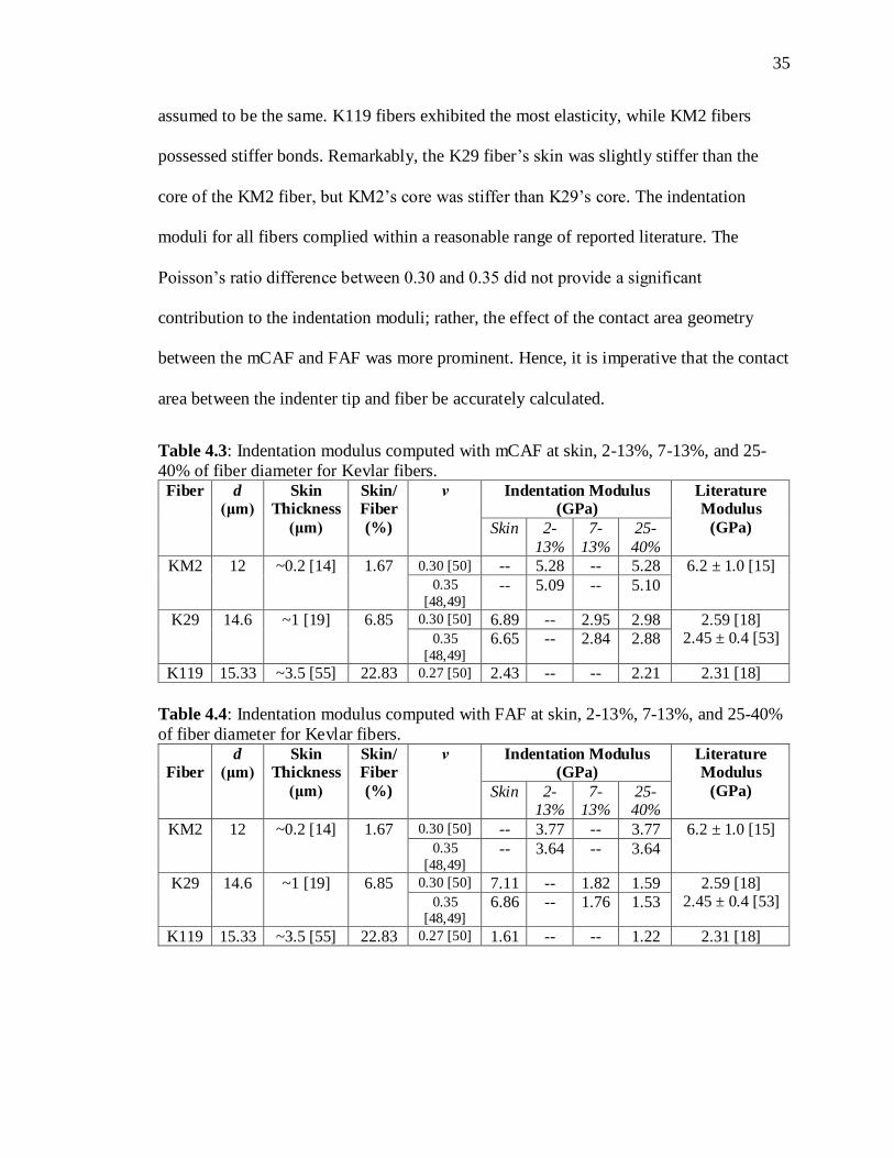
35
assumed to be the same. K119 fibers exhibited the most elasticity, while KM2 fibers
possessed stiffer bonds. Remarkably, the K29 fiber’s skin was slightly stiffer than the
core of the KM2 fiber, but KM2’s core was stiffer than K29’s core. The indentation
moduli for all fibers complied within a reasonable range of reported literature. The
Poisson’s ratio difference between 0.30 and 0.35 did not provide a significant
contribution to the indentation moduli; rather, the effect of the contact area geometry
between the mCAF and FAF was more prominent. Hence, it is imperative that the contact
area between the indenter tip and fiber be accurately calculated.
Table 4.3: Indentation modulus computed with mCAF at skin, 2-13%, 7-13%, and 25-
40% of fiber diameter for Kevlar fibers. Fiber d
(μm) Skin
Thickness
(μm)
Skin/Fiber
(%)
ν Indentation Modulus (GPa)
Literature Modulus
(GPa) Skin 2-
13%
7-
13%
25-
40%
KM2 12 ~0.2 [14] 1.67 0.30 [50] -- 5.28 -- 5.28 6.2 ± 1.0 [15] 0.35
[48,49] -- 5.09 -- 5.10
K29 14.6 ~1 [19] 6.85 0.30 [50] 6.89 -- 2.95 2.98 2.59 [18] 2.45 ± 0.4 [53] 0.35
[48,49] 6.65 -- 2.84 2.88
K119 15.33 ~3.5 [55] 22.83 0.27 [50] 2.43 -- -- 2.21 2.31 [18]
Table 4.4: Indentation modulus computed with FAF at skin, 2-13%, 7-13%, and 25-40%
of fiber diameter for Kevlar fibers.
Fiber d
(μm) Skin
Thickness
(μm)
Skin/Fiber
(%)
ν Indentation Modulus (GPa)
Literature Modulus
(GPa) Skin 2-13%
7-13%
25-40%
KM2 12 ~0.2 [14] 1.67 0.30 [50] -- 3.77 -- 3.77 6.2 ± 1.0 [15] 0.35
[48,49] -- 3.64 -- 3.64
K29 14.6 ~1 [19] 6.85 0.30 [50] 7.11 -- 1.82 1.59 2.59 [18] 2.45 ± 0.4 [53] 0.35
[48,49] 6.86 -- 1.76 1.53
K119 15.33 ~3.5 [55] 22.83 0.27 [50] 1.61 -- -- 1.22 2.31 [18]
36
4.2.1 Kevlar K29 Fiber
Using nanoindentation, Bencomo-Cisneros and their research group reported the
average hardness for K29 as 1.3 ± 0.7 GPa at a maximum depth of 100 nm [17]. This
value was suspected to be the hardness of the skin because the maximum depth of 100nm
does not exceed the 1μm thick skin [19]. Therefore, their research study concluded no
differences between the skin and core of the fiber [17]. According to Wollbrett-Blitz’s
research group, there was a clear difference in mechanical properties between the skin
and core of the K29 fiber [19]. The data, in Tables 4.3 and 4.4, supported Wollbrett-
Blitz’s conclusion of moduli differences between the skin and core of the K29 fiber.
From measurement results, the hardness of K29 skin was 0.68 GPa, which fell within the
range reported by Bencomo-Cisneros and their research group [17].
The FAF data for the K29 fiber yielded a slightly higher skin modulus than the
mCAF. Contrarily, the mCAF yielded a higher indentation modulus for the fiber core in
comparison to the FAF. The moduli for K29 in Tables 4.3 and 4.4 are illustrated in Fig.
4.8 for visual comparison at different percentages along the fiber diameter. The
corresponding load-controlled hysteresis curves are in Appendix A for reference. The
skin indentation modulus was roughly more than twice its core modulus. Kawabata’s
results clearly aligned with the moduli at 7-13% and 25-40% of fiber diameter.
37
Figure 4.8: K29 indentation modulus at various percentages of fiber diameter.
The drastic difference in modulus between the skin and core of the fiber proved
that the skin was stronger and less elastic than the core. The skin indentation moduli from
both mCAF and FAF were neighboring values; however, an immense difference between
the two contact area functions stemmed from deeper depths. At the higher depths, the
mCAF indentation moduli for Poisson’s ratio of 0.30 had the maximum value, whereas
the FAF had the lowest. Generally, the indentation moduli calculated from the mCAF at
higher contact depths agreed fairly with the elastic modulus of 2.59 GPa from
compression tests [18]. Therefore, the mCAF was more significant at higher contact
depths, but area correction factors are still a requirement at lower contact depths for
improved accuracy.
0
1
2
3
4
5
6
7
8
Skin 7-13% of Fiber Diameter 25-40% of Fiber Diameter
Ind
enta
tio
n M
od
ulu
s (G
Pa)
K29 Indentation Modulus at Various Percentages of Fiber
Diameter
Flat Area ν = 0.30 mCAF ν = 0.30 Flat Area ν = 0.35 mCAF ν = 0.35 Kawabata [18]
38
4.2.2 Kevlar KM2 Fiber
The KM2 depth sections are divided into two depths: 2-13% and 25-40% of fiber
diameter (Fig. 4.9). The indentation values for both sections are nearly identical and was
a similar trend with the K29 fiber at higher depths. For reference, load-controlled
hysteresis curves for these experiments are shown in Appendix B.
Generally, the indentation moduli determined from the mCAF function was
higher and agreed reasonably with McAllister’s [15] indentation modulus of 6.2 ± 1.0
GPa. McAllister’s group [15] implemented a Berkovich indenter tip for indentation on
KM2 fibers, but they lacked an area correction factor in their calculations. On the other
hand, Cole’s group [16] conducted indentations on KM2 Plus fibers with a Berkovich tip
although their area correction factors involved a spheroconical tip. Cole’s group
calculated an indentation modulus of 7.74 ± 0.96 GPa for KM2 Plus and they additionally
identified the importance of area correction factors in nanoindentation theory [16].
Overall, the KM2 Plus fibers proved to be stiffer than the core of KM2 fibers.
39
Figure 4.9: KM2 indentation modulus at various percentages of fiber diameter.
4.2.3 Kevlar K119 Fiber
The K119 fiber was distinct from the K29 and KM2 fibers because the skin
indentation moduli were closer to those of the core. Data from the FAF had the lowest
value for the skin in comparison to that from the mCAF and Kawabata’s elastic modulus
value of 2.31 GPa [18] (Fig. 4.10). The load-controlled hysteresis curves corresponding
to indentation moduli for K119 presented in Tables 4.3 and 4.4 are plotted in Appendix
C. In this specific fiber type, the indentation modulus had a closer value to Kawabata’s
[18] for both the skin and core of the fiber using the mCAF. Although Kawabata [18]
conducted compression testing, the indentation moduli values extrapolated from the
mCAF provided similar values to that of literature.
0
1
2
3
4
5
6
7
8
2-13% of Fiber Diameter 25-40% of Fiber Diameter
Ind
enta
tio
n M
od
ulu
s (G
Pa)
KM2 Indentation Modulus at Various Percentages of
Fiber Diameter
Flat Area ν = 0.30 mCAF ν = 0.30 Flat Area ν = 0.35 mCAF ν = 0.35 McAllister [15]

40
Figure 4.10: K119 indentation modulus at various percentages of fiber diameter.
4.3 PDMS Experimental Results
The PDMS specimen was tested with single and multiple cycle indentation
loading. The single cycle tests were necessary to determine the quasi static indentation
modulus for literature comparison. Multiple cycle loading was utilized to study frequency
dependency in the polymer. The surface roughness of this hydrophilic elastomer was very
little since it was molded with glass slides, but still varied at the nanoscale range. PDMS
is a very soft polymer with a Poisson’s ratio of 0.5 with incompressible characteristics at
room temperature [21, 56], hence very low loads were tested (Table 4.5).
Table 4.5: Two nanoindentation methods listed with the load-controlled tests on PDMS.
Load (mN) Single cycle
loading
Multiple cycle
loading
1 X X
2 X X
3 X X
4 X
0
0.5
1
1.5
2
2.5
3
Skin 25-40% of Fiber Diameter
Ind
enta
tio
n M
od
ulu
s (G
Pa)
K119 Indentation Modulus at Various Percentages of
Fiber Diameter
Flat Area mCAF Kawabata [18]

41
4.3.1 PDMS – Single Cycle Loading
Low loads of 1mN resulted in a high displacement of 8,310nm further proving
this material to be very soft with a low stiffness (Fig. 4.11(a)). This maximum depth was
significantly larger than the depth for K29 fibers at 1mN. PDMS was characterized to
have a very low indentation modulus compared to any of the Kevlar fibers. Specifically,
the average indentation modulus for PDMS was 5.45 ± 0.05 MPa at 1mN.
(a) (b)
(c) (d)
Figure 4.11: PDMS single cycle nanoindentation at (a) 1mN (8 curves), (b) 2mN (10
curves), (c) 3mN (10 curves), and (d) 4mN (10 curves).
The indenter tip reached a maximum average depth of 13,200nm at 2mN and the
average indentation modulus at this depth was a slight decrease from the average

42
indentation modulus at 1mN (Fig. 4.11(b)). The load-controlled indentations at 3mN had
an average maximum depth of 17,200nm, only at 1.72% of the specimen’s thickness. The
hysteresis curves at 3mN in Fig. 4.11(c) included 10 indents, which were used to
determine the stiffness. Similarly, the 4mN load-controlled indents reached an average
maximum depth of 20,300nm, which was 2.03% of the film thickness. The average
indentation modulus at this depth decreased to 3.76 ± 0.04 MPa and their hysteresis
curves are shown in Fig. 4.11(d).
Table 4.6: PDMS characterization of indentation modulus and hardness over a range of
depths through 1mm specimen thickness.
Load (mN)
Average
Maximum
Depth (nm)
Percentage of
Thickness (%)
Indentation
Modulus (MPa)
Hardness
(MPa)
1 8,310 ± 100 0.831 5.45 ± 0.05 2.1 ± 0.15
2 13,200 ± 109 1.32 4.37 ± 0.1 1.4 ± 0.12
3 17,200 ± 225 1.72 3.94 ± 0.06 1.2 ± 0.02
4 20,300 ± 250 2.03 3.76 ± 0.04 1.1 ± 0.04
The average indentation moduli at given loads are listed in Table 4.6 along with
corresponding depths and hardness. The maximum percentage of depth characterized for
PDMS was 2.03% of the thickness. A visual representation of the average maximum
depths plotted with their analogous indentation moduli from Table 4.6 are displayed in
Fig. 4.12. The indentation modulus decreased as the average maximum depth increased
up to 2.03% of the specimen thickness. Similar trends in reduced modulus of pristine
PDMS were seen in Maji’s research data [22]. Their study included reduced moduli data
on different forms of PDMS. The indentation modulus of 5.84 ± 1.76 MPa at 500nm was
measured with a Berkovich tip [22] and was approximately 5.45 ± 0.05 MPa in the
present study corresponding to a depth of 8,310nm (Table 4.6). Although the depths
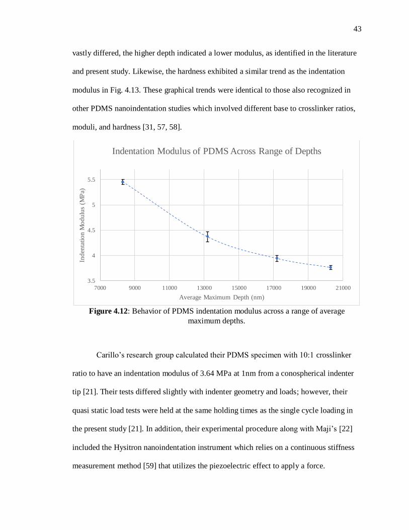
43
vastly differed, the higher depth indicated a lower modulus, as identified in the literature
and present study. Likewise, the hardness exhibited a similar trend as the indentation
modulus in Fig. 4.13. These graphical trends were identical to those also recognized in
other PDMS nanoindentation studies which involved different base to crosslinker ratios,
moduli, and hardness [31, 57, 58].
Figure 4.12: Behavior of PDMS indentation modulus across a range of average
maximum depths.
Carillo’s research group calculated their PDMS specimen with 10:1 crosslinker
ratio to have an indentation modulus of 3.64 MPa at 1nm from a conospherical indenter
tip [21]. Their tests differed slightly with indenter geometry and loads; however, their
quasi static load tests were held at the same holding times as the single cycle loading in
the present study [21]. In addition, their experimental procedure along with Maji’s [22]
included the Hysitron nanoindentation instrument which relies on a continuous stiffness
measurement method [59] that utilizes the piezoelectric effect to apply a force.
3.5
4
4.5
5
5.5
7000 9000 11000 13000 15000 17000 19000 21000
Ind
enta
tio
n M
od
ulu
s (M
Pa)
Average Maximum Depth (nm)
Indentation Modulus of PDMS Across Range of Depths

44
Conversely, the Vantage does not rely on this method because it uses a magnet and coils
to apply a force. These significant differences in experimental procedure explain small
discrepancies in data measurements. Overall, the data calculated from the Vantage at 3
and 4mN agree reasonably with the indentation modulus presented by literature [21].
Since data from Carillo [21] and Maji’s [22] group considerably agreed, indentation tests
validate data acquired on other specimens.
Figure 4.13: Behavior of PDMS hardness across a range of average maximum depths.
4.3.2 PDMS – Multiple Cycle Loading
During multiple cycle loading, the frequency was varied at three different load-
controlled experiments. At each frequency, the numbers of cycles were tabulated in Table
4.7 along with their corresponding indentation moduli minimum and maximum values.
Every frequency at a given load was tested with 5, 50, and 100 cycles each to study the
impact of varied cycles on indentation moduli and hardness. Three different frequencies
were tested to examine the influence of time dependency on the elastomer.
1
1.2
1.4
1.6
1.8
2
2.2
2.4
7000 9000 11000 13000 15000 17000 19000 21000
Har
dn
ess
(MP
a)
Average Maximum Depth (nm)
Hardness of PDMS Across Range of Depths

45
Table 4.7: Multiple cycle indentation load-controlled tests for PDMS at frequencies of 1,
0.5, and 0.033Hz. Each frequency test was performed with 5, 50, and 100 cycles. Each
test had a corresponding maximum and minimum indentation modulus.
Load
(mN)
Frequency
(Hz)
Cycles Es (MPa) Cycles Es (MPa) Cycles Es (MPa)
Min Max Min Max Min Max
1
1 5 6.34 6.64 50 5.64 6.20 100 5.28 6.14
0.5 5 6.42 6.70 50 5.38 5.96 100 4.98 6.10
0.033 5 5.26 5.68 50 2.60 5.40 100 1.58 5.28
2
1 5 5.02 5.26 50 4.64 5.10 100 4.34 4.94
0.5 5 4.92 5.12 50 4.38 4.86 100 4.12 4.94
0.033 5 4.08 4.48 50 2.24 4.4 100 1.50 4.50
3
1 5 4.48 4.72 50 4.20 4.56 100 4.02 4.52
0.5 5 4.38 4.56 50 3.96 4.36 100 3.70 4.40
0.033 5 3.72 4.02 50 2.14 4.06 100 1.38 3.88
Progressing from Fig. 4.14(a) to Fig 4.14(c), the loading and unloading curves
became smoother at 1mN load-controlled indents. This could be attributed by the
viscoelastic recovery which does not have time to stabilize at higher frequencies.
Although the bump (in Fig. 4.14(a) and (b)) from the loading curve between 0 and
1,000nm did not disappear in Fig 4.14(c), it still diminished and appeared stable. The
remainder of hysteresis multiple cycle loading curves are plotted in Appendix D and
exhibited similar trends in loading curves as those seen in Fig. 4.14.

46
(a) (b)
(c)
Figure 4.14: PDMS multiple cycle nanoindentation at 1mN and 5 cycles with varying
frequencies of (a) 1Hz (5 curves), (b) 0.5Hz (5 curves), (c) 0.033Hz (5 curves).
The maximum and minimum indentation moduli listed in Table 4.7 at 1mN for 5,
50, and 100 cycles were extracted from Fig. 4.15. The frequency decreased as the average
maximum depth increased and the relationship between this behavior was attributed to
creep. With a longer holding time, creep occurred and increased the maximum depth. In
higher frequencies, such as 1 and 0.5Hz, there was no dwell period at maximum load. A
lack of dwell period with a quick loading time prevented the polymer from viscoelastic
recovery and resulted in the jagged loading and unloading curves (Fig. 4.14(a) and (b)).
In Fig. 4.15, the 1 and 0.5Hz data were relatively at closer depths since large scale creep
did not occur as opposed to 0.033Hz loading tests. As the average maximum depth

47
increased, the indentation moduli slowly decreased in a power law trend. Increasing the
number of cycles increased the average maximum depth in the specimen. At 5 cycles,
most of the trends were linear since the difference in depths were not drastic. Conversely,
power law trends were clearly visible at 50 and 100 cycles.
The indentation moduli at 1mN were graphed for constant frequencies of 1, 0.5,
and 0.033Hz in Fig. 4.16. The lower cycles typically initiated at a lower average
maximum depth because it involved a combination of stress relaxation and surface
roughness. Indentation moduli also decreased with an increase in average maximum
depth in Fig. 4.16 because of energy loss. At smaller ranges in depth, indentation moduli
exhibited a linear trend with a negative slope (Fig. 4.16(a) and (b)). However, the larger
depths at 0.033Hz displayed a power law trend in respect to the indentation modulus, as
shown in Fig. 4.16(c). These patterns were also evident in the hardness in Fig. 4.17 (for
cycle trends) and 4.18 (for frequency trends). The load-controlled data yielded from 2
and 3mN indentations were graphed in the similar fashion as the 1mN load tests. The
indentation data at 2mN for constant cycles and frequencies are displayed in Fig. 4.19
and 4.20, respectively. The hardness graphs at 2mN are shown in Fig. 4.21 and 4.22.
Correspondingly, the 3mN load-controlled test data is depicted in Fig. 4.23 through 4.26.

48
(a)
(b)
(c)
Figure 4.15: PDMS indentation modulus graphs at 1mN with various frequencies at (a) 5
cycles, (b) 50 cycles, and (c) 100 cycles.
4.5
5
5.5
6
6.5
7
7400 7600 7800 8000 8200 8400 8600
Ind
enta
tio
n M
od
ulu
s (M
Pa)
Average Maximum Depth (nm)
PDMS Indentation Modulus at 1mN and 5 cycles
1Hz 0.5Hz 0.033Hz
2
2.5
3
3.5
4
4.5
5
5.5
6
6.5
7500 8500 9500 10500 11500 12500 13500
Ind
enta
tio
n M
od
ulu
s (M
Pa)
Average Maximum Depth (nm)
PDMS Indentation Modulus at 1mN and 50 cycles
1Hz 0.5Hz 0.033Hz
0
1
2
3
4
5
6
7
7000 9000 11000 13000 15000 17000 19000
Ind
enta
tio
n M
od
ulu
s (M
Pa)
Average Maximum Depth (nm)
PDMS Indentation Modulus at 1mN and 100 cycles
1Hz 0.5Hz 0.033Hz

49
(a)
(b)
(c) Figure 4.16: PDMS indentation modulus graphs at 1mN with various cycles at (a) 1Hz,
(b) 0.5Hz, and (c) 0.033Hz.
4
4.5
5
5.5
6
6.5
7
7400 7600 7800 8000 8200 8400 8600 8800
Ind
enta
tio
n M
od
ulu
s (M
Pa)
Average Maximum Depth (nm)
PDMS Indentation Modulus at 1mN and 1Hz
5 cycles 50 cycles 100 cycles
4
4.5
5
5.5
6
6.5
7
7400 7600 7800 8000 8200 8400 8600 8800 9000
Ind
enta
tio
n M
od
ulu
s (M
Pa)
Average Maximum Depth (nm)
PDMS Indentation Modulus at 1mN and 0.5Hz
5 cycles 50 cycles 100 cycles
1
1.5
2
2.5
3
3.5
4
4.5
5
5.5
6
8000 10000 12000 14000 16000 18000 20000
Ind
enta
tio
n M
od
ulu
s (M
Pa)
Average Maximum Depth (nm)
PDMS Indentation Modulus at 1mN and 0.033Hz
5 cycles 50 cycles 100 cycles
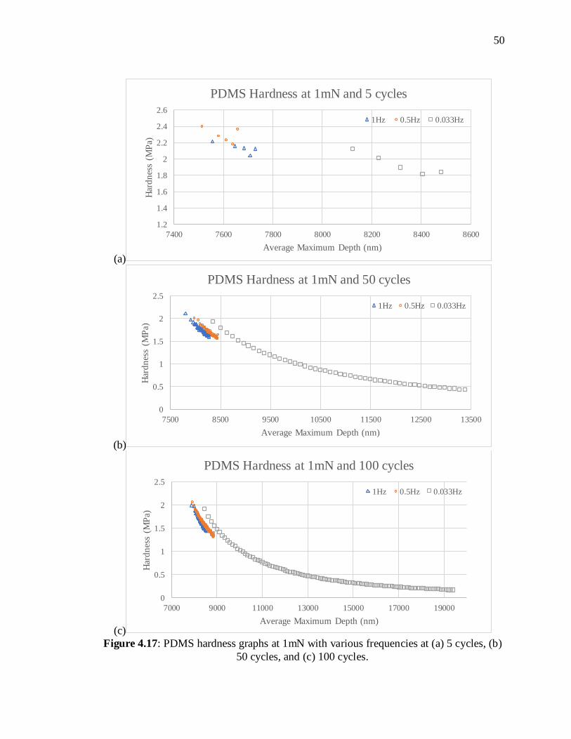
50
(a)
(b)
(c) Figure 4.17: PDMS hardness graphs at 1mN with various frequencies at (a) 5 cycles, (b)
50 cycles, and (c) 100 cycles.
1.2
1.4
1.6
1.8
2
2.2
2.4
2.6
7400 7600 7800 8000 8200 8400 8600
Har
dn
ess
(MP
a)
Average Maximum Depth (nm)
PDMS Hardness at 1mN and 5 cycles
1Hz 0.5Hz 0.033Hz
0
0.5
1
1.5
2
2.5
7500 8500 9500 10500 11500 12500 13500
Har
dn
ess
(MP
a)
Average Maximum Depth (nm)
PDMS Hardness at 1mN and 50 cycles
1Hz 0.5Hz 0.033Hz
0
0.5
1
1.5
2
2.5
7000 9000 11000 13000 15000 17000 19000
Har
dn
ess
(MP
a)
Average Maximum Depth (nm)
PDMS Hardness at 1mN and 100 cycles
1Hz 0.5Hz 0.033Hz

51
(a)
(b)
(c) Figure 4.18: PDMS hardness graphs at 1mN with various cycles at (a) 1Hz, (b) 0.5Hz,
and (c) 0.033Hz.
1
1.2
1.4
1.6
1.8
2
2.2
2.4
7400 7600 7800 8000 8200 8400 8600 8800
Har
dn
ess
(MP
a)
Average Maximum Depth (nm)
PDMS Hardness at 1mN and 1Hz
5 cycles 50 cycles 100 cycles
0
0.5
1
1.5
2
2.5
3
7400 7600 7800 8000 8200 8400 8600 8800 9000
Har
dn
ess
(MP
a)
Average Maximum Depth (nm)
PDMS Hardness at 1mN and 0.5Hz
5 cycles 50 cycles 100 cycles
0
0.5
1
1.5
2
2.5
7000 9000 11000 13000 15000 17000 19000
Har
dn
ess
(MP
a)
Average Maximum Depth (nm)
PDMS Hardness at 1mN and 0.033Hz
5 cycles 50 cycles 100 cycles
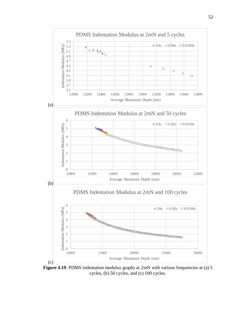
52
(a)
(b)
(c) Figure 4.19: PDMS indentation modulus graphs at 2mN with various frequencies at (a) 5
cycles, (b) 50 cycles, and (c) 100 cycles.
3.5
3.7
3.9
4.1
4.3
4.5
4.7
4.9
5.1
5.3
5.5
12000 12200 12400 12600 12800 13000 13200 13400 13600 13800
Ind
enta
tio
n M
od
ulu
s (M
Pa)
Average Maximum Depth (nm)
PDMS Indentation Modulus at 2mN and 5 cycles
1Hz 0.5Hz 0.033Hz
0
1
2
3
4
5
6
10000 12000 14000 16000 18000 20000 22000
Ind
enta
tio
n M
od
ulu
s (M
Pa)
Average Maximum Depth (nm)
PDMS Indentation Modulus at 2mN and 50 cycles
1Hz 0.5Hz 0.033Hz
0
1
2
3
4
5
6
10000 15000 20000 25000 30000
Ind
enta
tio
n M
od
ulu
s (M
Pa)
Average Maximum Depth (nm)
PDMS Indentation Modulus at 2mN and 100 cycles
1Hz 0.5Hz 0.033Hz

53
(a)
(b)
(c) Figure 4.20: PDMS indentation modulus graphs at 2mN with various cycles at (a) 1Hz,
(b) 0.5Hz, and (c) 0.033Hz.
4
4.2
4.4
4.6
4.8
5
5.2
5.4
12000 12200 12400 12600 12800 13000 13200 13400 13600
Ind
enta
tio
n M
od
ulu
s (M
Pa)
Average Maximum Depth (nm)
PDMS Indentation Modulus at 2mN and 1Hz
5 cycles 50 cycles 100 cycles
4
4.2
4.4
4.6
4.8
5
5.2
12000 12500 13000 13500 14000 14500
Ind
enta
tio
n M
od
ulu
s (M
Pa)
Average Maximum Depth (nm)
PDMS Indentation Modulus at 2mN and 0.5Hz
5 cycles 50 cycles 100 cycles
1
1.5
2
2.5
3
3.5
4
4.5
5
12000 14000 16000 18000 20000 22000 24000 26000 28000
Ind
enta
tio
n M
od
ulu
s (M
Pa)
Average Maximum Depth (nm)
PDMS Indentation Modulus at 2mN and 0.033Hz
5 cycles 50 cycles 100 cycles
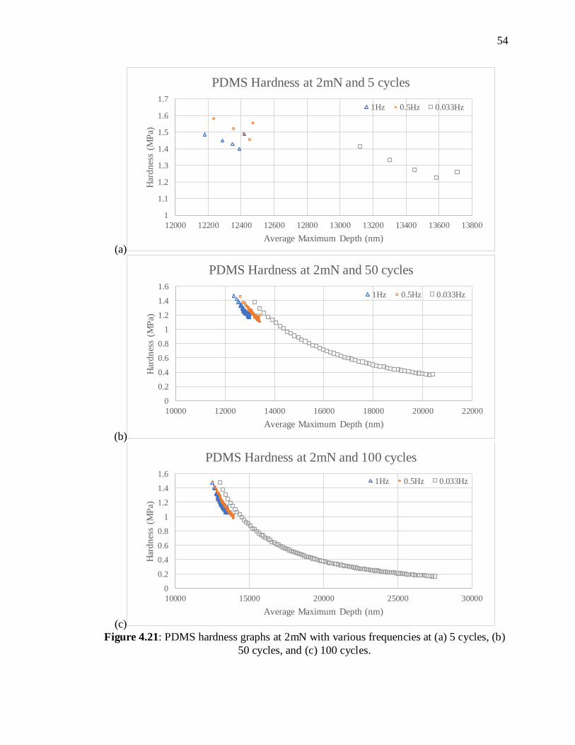
54
(a)
(b)
(c) Figure 4.21: PDMS hardness graphs at 2mN with various frequencies at (a) 5 cycles, (b)
50 cycles, and (c) 100 cycles.
1
1.1
1.2
1.3
1.4
1.5
1.6
1.7
12000 12200 12400 12600 12800 13000 13200 13400 13600 13800
Har
dn
ess
(MP
a)
Average Maximum Depth (nm)
PDMS Hardness at 2mN and 5 cycles
1Hz 0.5Hz 0.033Hz
0
0.2
0.4
0.6
0.8
1
1.2
1.4
1.6
10000 12000 14000 16000 18000 20000 22000
Har
dn
ess
(MP
a)
Average Maximum Depth (nm)
PDMS Hardness at 2mN and 50 cycles
1Hz 0.5Hz 0.033Hz
0
0.2
0.4
0.6
0.8
1
1.2
1.4
1.6
10000 15000 20000 25000 30000
Har
dn
ess
(MP
a)
Average Maximum Depth (nm)
PDMS Hardness at 2mN and 100 cycles
1Hz 0.5Hz 0.033Hz
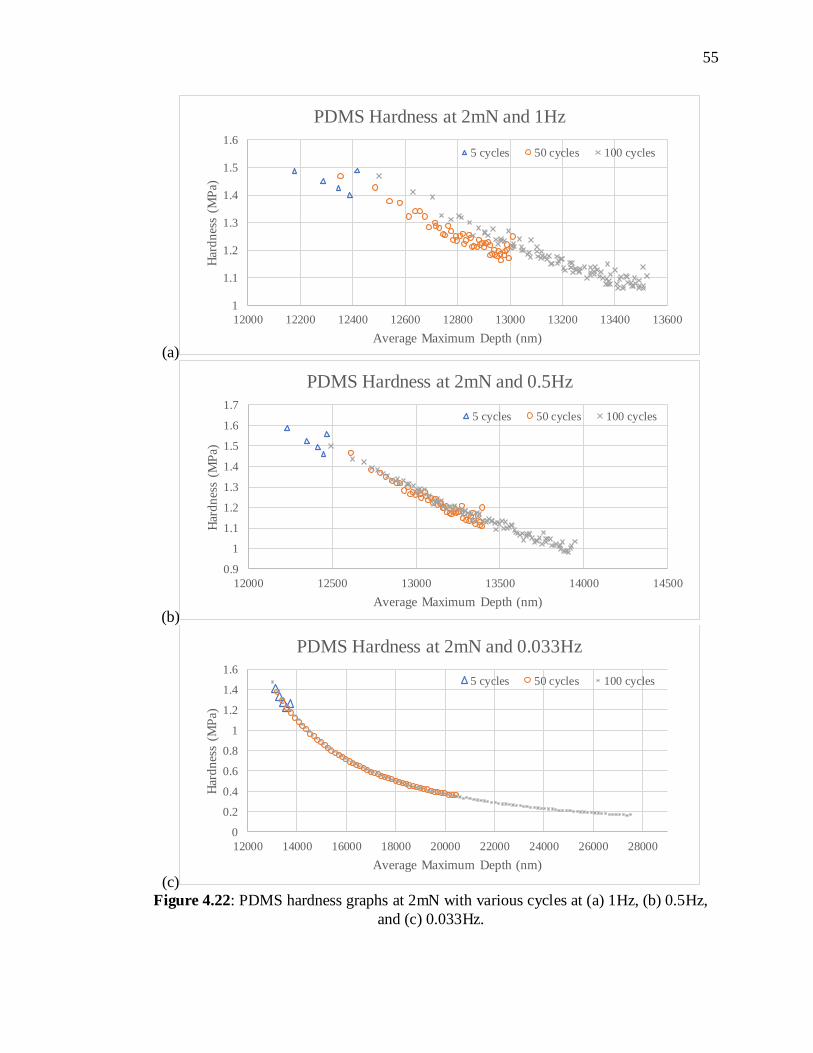
55
(a)
(b)
(c) Figure 4.22: PDMS hardness graphs at 2mN with various cycles at (a) 1Hz, (b) 0.5Hz,
and (c) 0.033Hz.
1
1.1
1.2
1.3
1.4
1.5
1.6
12000 12200 12400 12600 12800 13000 13200 13400 13600
Har
dn
ess
(MP
a)
Average Maximum Depth (nm)
PDMS Hardness at 2mN and 1Hz
5 cycles 50 cycles 100 cycles
0.9
1
1.1
1.2
1.3
1.4
1.5
1.6
1.7
12000 12500 13000 13500 14000 14500
Har
dn
ess
(MP
a)
Average Maximum Depth (nm)
PDMS Hardness at 2mN and 0.5Hz
5 cycles 50 cycles 100 cycles
0
0.2
0.4
0.6
0.8
1
1.2
1.4
1.6
12000 14000 16000 18000 20000 22000 24000 26000 28000
Har
dn
ess
(MP
a)
Average Maximum Depth (nm)
PDMS Hardness at 2mN and 0.033Hz
5 cycles 50 cycles 100 cycles

56
(a)
(b)
(c) Figure 4.23: PDMS indentation modulus graphs at 3mN with various frequencies at (a) 5
cycles, (b) 50 cycles, and (c) 100 cycles.
3.6
3.8
4
4.2
4.4
4.6
4.8
15500 16000 16500 17000 17500 18000
Ind
enta
tio
n M
od
ulu
s (M
Pa)
Average Maximum Depth (nm)
PDMS Indentation Modulus at 3mN and 5 cycles
1Hz 0.5Hz 0.033Hz
2
2.5
3
3.5
4
4.5
5
15000 17000 19000 21000 23000 25000 27000
Ind
enta
tio
n M
od
ulu
s (M
Pa)
Average Maximum Depth (nm)
PDMS Indentation Modulus at 3mN and 50 cycles
1Hz 0.5Hz 0.033Hz
0
0.5
1
1.5
2
2.5
3
3.5
4
4.5
5
15000 20000 25000 30000 35000 40000
Ind
enta
tio
n M
od
ulu
s (M
Pa)
Average Maximum Depth (nm)
PDMS Indentation Modulus at 3mN and 100 cycles
1Hz 0.5Hz 0.033Hz
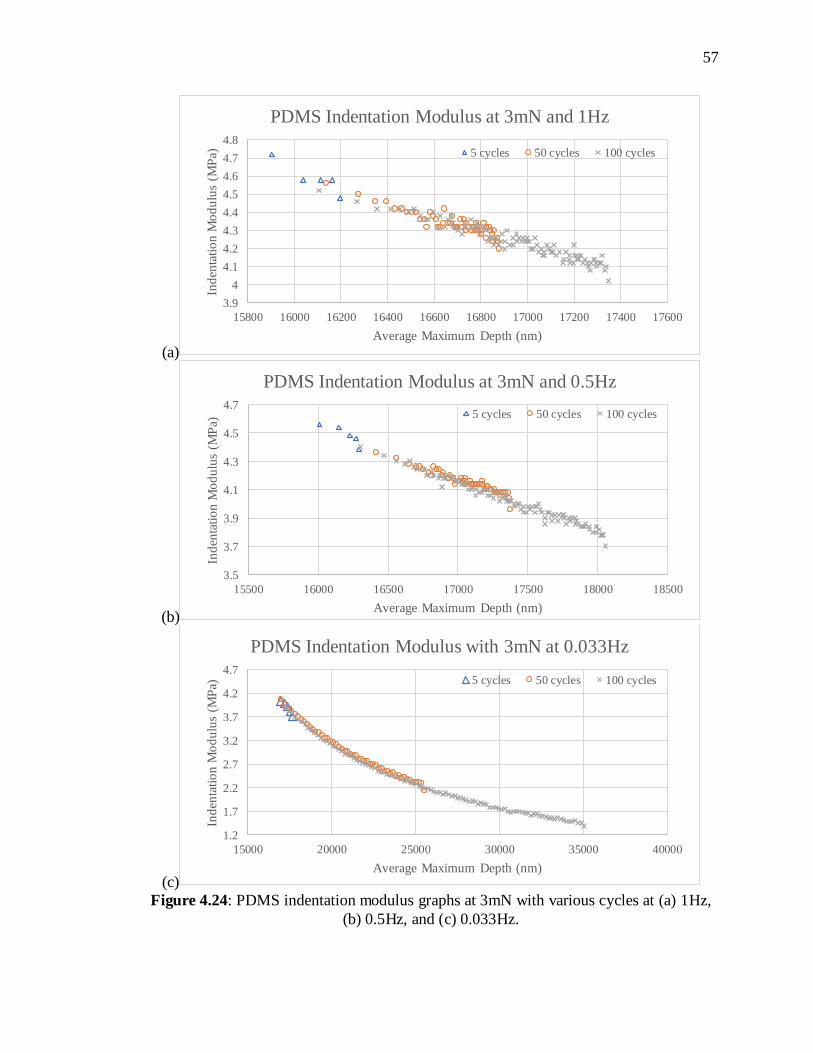
57
(a)
(b)
(c) Figure 4.24: PDMS indentation modulus graphs at 3mN with various cycles at (a) 1Hz,
(b) 0.5Hz, and (c) 0.033Hz.
3.9
4
4.1
4.2
4.3
4.4
4.5
4.6
4.7
4.8
15800 16000 16200 16400 16600 16800 17000 17200 17400 17600
Ind
enta
tio
n M
od
ulu
s (M
Pa)
Average Maximum Depth (nm)
PDMS Indentation Modulus at 3mN and 1Hz
5 cycles 50 cycles 100 cycles
3.5
3.7
3.9
4.1
4.3
4.5
4.7
15500 16000 16500 17000 17500 18000 18500
Ind
enta
tio
n M
od
ulu
s (M
Pa)
Average Maximum Depth (nm)
PDMS Indentation Modulus at 3mN and 0.5Hz
5 cycles 50 cycles 100 cycles
1.2
1.7
2.2
2.7
3.2
3.7
4.2
4.7
15000 20000 25000 30000 35000 40000
Ind
enta
tio
n M
od
ulu
s (M
Pa)
Average Maximum Depth (nm)
PDMS Indentation Modulus with 3mN at 0.033Hz
5 cycles 50 cycles 100 cycles

58
(a)
(b)
(c) Figure 4.25: PDMS hardness graphs at 3mN with various frequencies at (a) 5 cycles, (b)
50 cycles, and (c) 100 cycles.
1
1.05
1.1
1.15
1.2
1.25
1.3
1.35
15500 16000 16500 17000 17500 18000
Har
dn
ess
(MP
a)
Average Maximum Depth (nm)
PDMS Hardness at 3mN and 5 cycles
1Hz 0.5Hz 0.033Hz
0.2
0.4
0.6
0.8
1
1.2
1.4
15000 17000 19000 21000 23000 25000 27000
Har
dn
ess
(MP
a)
Average Maximum Depth (nm)
PDMS Hardness at 3mN and 50 cycles
1Hz 0.5Hz 0.033Hz
0
0.2
0.4
0.6
0.8
1
1.2
1.4
15000 20000 25000 30000 35000 40000
Har
dn
ess
(MP
a)
Average Maximum Depth (nm)
PDMS Hardness at 3mN and 100 cycles
1Hz 0.5Hz 0.033Hz

59
(a)
(b)
(c) Figure 4.26: PDMS hardness graphs at 3mN with various cycles at (a) 1Hz, (b) 0.5Hz,
and (c) 0.033Hz.
0.8
0.85
0.9
0.95
1
1.05
1.1
1.15
1.2
1.25
1.3
15800 16000 16200 16400 16600 16800 17000 17200 17400 17600
Har
dn
ess
(MP
a)
Average Maximum Depth (nm)
PDMS Hardness at 3mN and 1Hz
5 cycles 50 cycles 100 cycles
0.8
0.9
1
1.1
1.2
1.3
1.4
15500 16000 16500 17000 17500 18000 18500
Har
dn
ess
(MP
a)
Average Maximum Depth (nm)
PDMS Hardness at 3mN and 0.5Hz
5 cycles 50 cycles 100 cycles
0
0.2
0.4
0.6
0.8
1
1.2
1.4
15000 20000 25000 30000 35000 40000
Har
dn
ess
(MP
a)
Average Maximum Depth (nm)
PDMS Hardness at 3mN and 0.033Hz
5 cycles 50 cycles 100 cycles

60
4.4 SMP Experimental Results
Two types of indentation methods were tested on the SMP specimens. The first
method involved single cycle loading and was conducted at the following load-controlled
tests listed in Table 4.8. Three different loads: 3, 10, and 50mN were specifically selected
for studying frequency dependency in multiple cycle loading. The variety in loads
provided an assortment of data ranging from low to high loads. From laboratory dynamic
mechanical analysis (DMA) testing, the Poisson’s ratio was specifically estimated as 0.44
for this hydrophilic specimen.
Table 4.8: Two nanoindentation methods listed with the load-controlled tests on SMP.
Load (mN) Single cycle loading Multiple cycle loading
2 X
3 X X
4 X
5 X
10 X X
20 X
30 X
50 X X
100 X
200 X
250 X
300 X
4.4.1 SMP – Single Cycle Loading
Although its softness did not compare to the PDMS, the SMP was able to resist
higher loads to collect more load-controlled data. Indentations from 2 to 300mN were
completed on the SMP (Table 4.8) and single cycle loading curves at 2, 3, 4, and 5mN
are shown in Fig. 4.27.
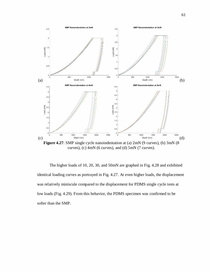
61
(a) (b)
(c) (d)
Figure 4.27: SMP single cycle nanoindentation at (a) 2mN (9 curves), (b) 3mN (8
curves), (c) 4mN (6 curves), and (d) 5mN (7 curves).
The higher loads of 10, 20, 30, and 50mN are graphed in Fig. 4.28 and exhibited
identical loading curves as portrayed in Fig. 4.27. At even higher loads, the displacement
was relatively miniscule compared to the displacement for PDMS single cycle tests at
low loads (Fig. 4.29). From this behavior, the PDMS specimen was confirmed to be
softer than the SMP.

62
(a) (b)
(c) (d)
Figure 4.28: SMP single cycle nanoindentation at (a) 10mN (5 curves), (b) 20mN (10
curves), (c) 30mN (10 curves), and (d) 50mN (9 curves).
The corresponding indentation moduli, hardness, and depths for each set of loads
was organized in Table 4.9. The depth was compared to the thickness of the specimen
and was provided as a percentage in that table. The maximum load of 300mN only
pierced about 1.937% of the specimen’s thickness, whereas only a 4mN load test reached
roughly the same percentage in the PDMS. This drastic comparison portrays the SMP as
a stronger and vigorous specimen which can resist higher loads. PDMS ultimately
exhibited more elasticity than the SMP because of its low indentation modulus.

63
(a) (b)
(c) (d)
Figure 4.29: SMP single cycle nanoindentation at (a) 100mN (6 curves), (b) 200mN (10
curves), (c) 250mN (10 curves), and (d) 300mN (8 curves).
At a range from 1,342nm to 4,108nm, the indentation modulus was relatively
constant around 2 GPa, but decreased as the depth increased. Although the decrease was
not as consistent as the behavior in PDMS, the SMP had its lowest measured indentation
modulus of 1.62 GPa at 19,374nm. The hardness did not display a similar decreasing
trend, instead it remained around 0.044 GPa. Small fluctuations in surface area and stress
relaxation were likely culprits of this discrepancy. The polymer was generally able to
creep and conform to the indentation load, displaying smooth loading and unloading
curves in Fig. 4.27 through 4.29.
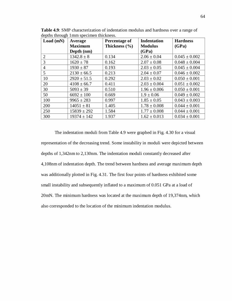
64
Table 4.9: SMP characterization of indentation modulus and hardness over a range of
depths through 1mm specimen thickness.
Load (mN) Average
Maximum
Depth (nm)
Percentage of
Thickness (%)
Indentation
Modulus
(GPa)
Hardness
(GPa)
2 1342.8 ± 8 0.134 2.06 ± 0.04 0.045 ± 0.002
3 1620 ± 78 0.162 2.07 ± 0.08 0.048 ± 0.004
4 1930 ± 87 0.193 2.03 ± 0.05 0.045 ± 0.004
5 2130 ± 66.5 0.213 2.04 ± 0.07 0.046 ± 0.002
10 2920 ± 51.5 0.292 2.03 ± 0.02 0.050 ± 0.001
20 4108 ± 66.7 0.411 2.03 ± 0.004 0.051 ± 0.002
30 5093 ± 39 0.510 1.96 ± 0.006 0.050 ± 0.001
50 6692 ± 100 0.669 1.9 ± 0.06 0.049 ± 0.002
100 9965 ± 283 0.997 1.85 ± 0.05 0.043 ± 0.003
200 14051 ± 81 1.405 1.78 ± 0.008 0.044 ± 0.001
250 15839 ± 292 1.584 1.77 ± 0.008 0.044 ± 0.001
300 19374 ± 142 1.937 1.62 ± 0.013 0.034 ± 0.001
The indentation moduli from Table 4.9 were graphed in Fig. 4.30 for a visual
representation of the decreasing trend. Some instability in moduli were depicted between
depths of 1,342nm to 2,130nm. The indentation moduli constantly decreased after
4,108nm of indentation depth. The trend between hardness and average maximum depth
was additionally plotted in Fig. 4.31. The first four points of hardness exhibited some
small instability and subsequently inflated to a maximum of 0.051 GPa at a load of
20mN. The minimum hardness was located at the maximum depth of 19,374nm, which
also corresponded to the location of the minimum indentation modulus.
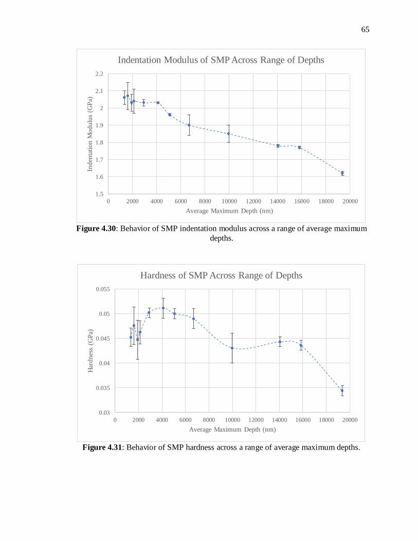
65
Figure 4.30: Behavior of SMP indentation modulus across a range of average maximum
depths.
Figure 4.31: Behavior of SMP hardness across a range of average maximum depths.
1.5
1.6
1.7
1.8
1.9
2
2.1
2.2
0 2000 4000 6000 8000 10000 12000 14000 16000 18000 20000
Ind
enta
tio
n M
od
ulu
s (G
Pa)
Average Maximum Depth (nm)
Indentation Modulus of SMP Across Range of Depths
0.03
0.035
0.04
0.045
0.05
0.055
0 2000 4000 6000 8000 10000 12000 14000 16000 18000 20000
Har
dn
ess
(GP
a)
Average Maximum Depth (nm)
Hardness of SMP Across Range of Depths
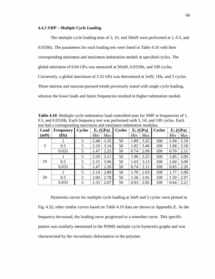
66
4.4.2 SMP – Multiple Cycle Loading
The multiple cycle loading tests of 3, 10, and 50mN were performed at 1, 0.5, and
0.033Hz. The parameters for each loading test were listed in Table 4.10 with their
corresponding minimum and maximum indentation moduli at specified cycles. The
global minimum of 0.64 GPa was measured at 50mN, 0.033Hz, and 100 cycles.
Conversely, a global maximum of 3.35 GPa was determined at 3mN, 1Hz, and 5 cycles.
These minima and maxima pursued trends previously stated with single cycle loading,
whereas the lower loads and faster frequencies resulted in higher indentation moduli.
Table 4.10: Multiple cycle indentation load-controlled tests for SMP at frequencies of 1,
0.5, and 0.033Hz. Each frequency test was performed with 5, 50, and 100 cycles. Each
test had a corresponding maximum and minimum indentation modulus.
Load
(mN)
Frequency
(Hz)
Cycles Es (GPa) Cycles Es (GPa) Cycles Es (GPa)
Min Max Min Max Min Max
3
1 5 2.48 3.35 50 1.89 3.25 100 1.94 3.19
0.5 5 2.19 3.14 50 1.82 3.40 100 1.68 3.18
0.033 5 1.47 2.25 50 0.74 2.09 100 0.70 2.11
10
1 5 2.29 3.11 50 1.90 3.25 100 1.85 3.09
0.5 5 2.15 3.06 50 1.63 3.13 100 1.60 3.09
0.033 5 1.47 2.20 50 0.74 2.11 100 0.65 2.26
50
1 5 2.14 2.89 50 1.70 2.93 100 1.77 3.00
0.5 5 2.00 2.78 50 1.56 2.91 100 1.50 2.97
0.033 5 1.33 2.07 50 0.93 2.82 100 0.64 2.21
Hysteresis curves for multiple cycle loading at 3mN and 5 cycles were plotted in
Fig. 4.32; other similar curves based on Table 4.10 data are shown in Appendix E. As the
frequency decreased, the loading curve progressed to a smoother curve. This specific
pattern was similarly mentioned in the PDMS multiple cycle hysteresis graphs and was
characterized by the viscoelastic deformation in the polymer.

67
(a) (b)
(c)
Figure 4.32: SMP multiple cycle nanoindentation at 3mN and 5 cycles with varying
frequencies of (a) 1Hz (7 curves), (b) 0.5Hz (7 curves), (c) 0.033Hz (7 curves).
The indentation moduli corresponding to 3mN load tests in Table 4.10 at each
cycle and frequency were plotted in Fig. 4.33 and 4.34, respectively. The surface
roughness of the SMP was more significant compared to PDMS due to the SMP’s
hydrophilic characteristics. Again, indentation moduli continued to decrease as maximum
depth increased because of energy loss associated with friction and loss modulus. This
was also analogous to the hardness trends at 3mN loads in Fig. 4.35 and 4.36. The
indentation moduli maxima and minima from Table 4.10 for 3, 10, and 50mN were
extracted from Fig. 4.33 through 4.44. The patterns for each of these graphs were
comparable to those from PDMS, except mechanical properties for the SMP were

68
measured at greater magnitudes and lower depths. Tests of 5 cycles typically had a linear
trend for PDMS, whereas it was not visible in the SMP tests (Fig. 4.33(a), 4.35(a),
4.37(a), 4.39(a), 4.41(a), and 4.43(a)). The 50 and 100 cycle tests exhibited power law
curves, similarly to the PDMS tests. All frequency consistent graphs (Fig. 4.34, 4.36,
4.38, 3.40, 3.42, and 3.44) portrayed power law or even exponential decay trends, as
opposed to the PDMS where the only graphs with power law trends were 0.033Hz tests.
For PDMS curves, the 1 and 0.5Hz graphs generally exhibited linearity in data points.
These differences in trends outline differences in both polymers, even though there were
similarities in viscoelastic behavior.

69
(a)
(b)
(c) Figure 4.33: SMP indentation modulus graphs at 3mN with various frequencies at (a) 5
cycles, (b) 50 cycles, and (c) 100 cycles.
1
1.5
2
2.5
3
3.5
1000 1500 2000 2500 3000
Ind
enta
tio
n M
od
ulu
s (G
Pa)
Average Maximum Depth (nm)
SMP Indentation Modulus at 3mN and 5 cycles
1Hz 0.5Hz 0.033Hz
0
0.5
1
1.5
2
2.5
3
3.5
4
0 1000 2000 3000 4000 5000 6000 7000 8000
Ind
enta
tio
n M
od
ulu
s (G
Pa)
Average Maximum Depth (nm)
SMP Indentation Modulus at 3mN and 50 cycles
1Hz 0.5Hz 0.033Hz
0
0.5
1
1.5
2
2.5
3
3.5
0 2000 4000 6000 8000 10000
Ind
enta
tio
n M
od
ulu
s (G
Pa)
Average Maximum Depth (nm)
SMP Indentation Modulus at 3mN and 100
cycles
1Hz 0.5Hz 0.033Hz

70
(a)
(b)
(c) Figure 4.34: SMP indentation modulus graphs at 3mN with various cycles at (a) 1Hz, (b)
0.5Hz, and (c) 0.033Hz.
1.5
1.7
1.9
2.1
2.3
2.5
2.7
2.9
3.1
3.3
3.5
1000 1200 1400 1600 1800 2000 2200
Ind
enta
tio
n M
od
ulu
s (G
Pa)
Average Maximum Depth (nm)
SMP Indentation Modulus at 3mN and 1Hz
5 cycles 50 cycles 100 cycles
1.5
1.7
1.9
2.1
2.3
2.5
2.7
2.9
3.1
3.3
3.5
1000 1200 1400 1600 1800 2000 2200 2400 2600
Ind
enta
tio
n M
od
ulu
s (G
Pa)
Average Maximum Depth (nm)
SMP Indentation Modulus at 3mN and 0.5Hz
5 cycles 50 cycles 100 cycles
0.5
0.7
0.9
1.1
1.3
1.5
1.7
1.9
2.1
2.3
2.5
1000 2000 3000 4000 5000 6000 7000 8000 9000
Ind
enta
tio
n M
od
ulu
s (G
Pa)
Average Maximum Depth (nm)
SMP Indentation Modulus at 3mN and 0.033Hz
5 cycles 50 cycles 100 cycles

71
(a)
(b)
(c) Figure 4.35: SMP hardness graphs at 3mN with various frequencies at (a) 5 cycles, (b)
50 cycles, and (c) 100 cycles.
0
0.02
0.04
0.06
0.08
0.1
0.12
0.14
1000 1200 1400 1600 1800 2000 2200 2400 2600 2800
Har
dn
ess
(GP
a)
Average Maximum Depth (nm)
SMP Hardness at 3mN and 5 cycles
1Hz 0.5Hz 0.033Hz
0
0.02
0.04
0.06
0.08
0.1
0.12
0.14
0 1000 2000 3000 4000 5000 6000 7000 8000
Har
dn
ess
(GP
a)
Average Maximum Depth (nm)
SMP Hardness at 3mN and 50 cycles
1Hz 0.5Hz 0.033Hz
0
0.02
0.04
0.06
0.08
0.1
0.12
0 1000 2000 3000 4000 5000 6000 7000 8000 9000
Har
dn
ess
(GP
a)
Average Maximum Depth (nm)
SMP Hardness at 3mN and 100 cycles
1Hz 0.5Hz 0.033Hz

72
(a)
(b)
(c) Figure 4.36: SMP hardness graphs at 3mN with various cycles at (a) 1Hz, (b) 0.5Hz, and
(c) 0.033Hz.
0
0.02
0.04
0.06
0.08
0.1
0.12
0.14
1000 1200 1400 1600 1800 2000 2200
Har
dn
ess
(GP
a)
Average Maximum Depth (nm)
SMP Hardness at 3mN and 1Hz
5 cycles 50 cycles 100 cycles
0
0.02
0.04
0.06
0.08
0.1
0.12
0.14
1000 1200 1400 1600 1800 2000 2200 2400 2600
Ind
enta
tio
n M
od
ulu
s (G
Pa)
Average Maximum Depth (nm)
SMP Hardness at 3mN and 0.5Hz
5 cycles 50 cycles 100 cycles
0
0.005
0.01
0.015
0.02
0.025
0.03
0.035
0.04
0.045
1000 2000 3000 4000 5000 6000 7000 8000 9000
Har
dn
ess
(GP
a)
Average Maximum Depth (nm)
SMP Hardness at 3mN and 0.033Hz
5 cycles 50 cycles 100 cycles
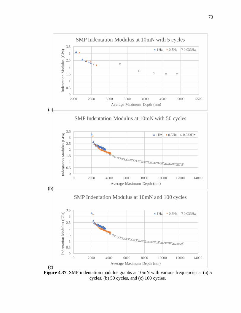
73
(a)
(b)
(c) Figure 4.37: SMP indentation modulus graphs at 10mN with various frequencies at (a) 5
cycles, (b) 50 cycles, and (c) 100 cycles.
0
0.5
1
1.5
2
2.5
3
3.5
2000 2500 3000 3500 4000 4500 5000 5500
Ind
enta
tio
n M
od
ulu
s (G
Pa)
Average Maximum Depth (nm)
SMP Indentation Modulus at 10mN with 5 cycles
1Hz 0.5Hz 0.033Hz
0
0.5
1
1.5
2
2.5
3
3.5
0 2000 4000 6000 8000 10000 12000 14000
Ind
enta
tio
n M
od
ulu
s (G
Pa)
Average Maximum Depth (nm)
SMP Indentation Modulus at 10mN with 50 cycles
1Hz 0.5Hz 0.033Hz
0
0.5
1
1.5
2
2.5
3
3.5
0 2000 4000 6000 8000 10000 12000 14000
Ind
enta
tio
n M
od
ulu
s (G
Pa)
Average Maximum Depth (nm)
SMP Indentation Modulus at 10mN and 100 cycles
1Hz 0.5Hz 0.033Hz
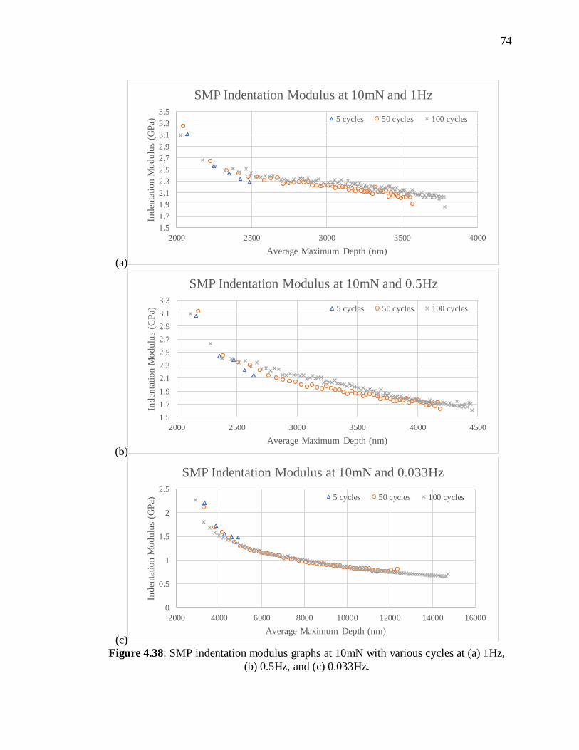
74
(a)
(b)
(c) Figure 4.38: SMP indentation modulus graphs at 10mN with various cycles at (a) 1Hz,
(b) 0.5Hz, and (c) 0.033Hz.
1.5
1.7
1.9
2.1
2.3
2.5
2.7
2.9
3.1
3.3
3.5
2000 2500 3000 3500 4000
Ind
enta
tio
n M
od
ulu
s (G
Pa)
Average Maximum Depth (nm)
SMP Indentation Modulus at 10mN and 1Hz
5 cycles 50 cycles 100 cycles
1.5
1.7
1.9
2.1
2.3
2.5
2.7
2.9
3.1
3.3
2000 2500 3000 3500 4000 4500
Ind
enta
tio
n M
od
ulu
s (G
Pa)
Average Maximum Depth (nm)
SMP Indentation Modulus at 10mN and 0.5Hz
5 cycles 50 cycles 100 cycles
0
0.5
1
1.5
2
2.5
2000 4000 6000 8000 10000 12000 14000 16000
Ind
enta
tio
n M
od
ulu
s (G
Pa)
Average Maximum Depth (nm)
SMP Indentation Modulus at 10mN and 0.033Hz
5 cycles 50 cycles 100 cycles

75
(a)
(b)
(c) Figure 4.39: SMP hardness graphs at 10mN with various frequencies at (a) 5 cycles, (b)
50 cycles, and (c) 100 cycles.
0
0.02
0.04
0.06
0.08
0.1
0.12
2000 2500 3000 3500 4000 4500 5000 5500
Har
dn
ess
(GP
a)
Average Maximum Depth (nm)
SMP Hardness at 10mN and 5 cycles
1Hz 0.5Hz 0.033Hz
0
0.02
0.04
0.06
0.08
0.1
0.12
0 2000 4000 6000 8000 10000 12000 14000
Har
dn
ess
(GP
a)
Average Maximum Depth (nm)
SMP Hardness at 10mN and 50 cycles
1Hz 0.5Hz 0.033Hz
0
0.5
1
1.5
2
2.5
3
3.5
0 2000 4000 6000 8000 10000 12000 14000
Ind
enta
tio
n M
od
ulu
s (G
Pa)
Average Maximum Depth (nm)
SMP Indentation Modulus at 10mN and 100 cycles
1Hz 0.5Hz 0.033Hz
76
(a)
(b)
(c) Figure 4.40: SMP hardness graphs at 10mN with various cycles at (a) 1Hz, (b) 0.5Hz,
and (c) 0.033Hz.
0.02
0.03
0.04
0.05
0.06
0.07
0.08
0.09
0.1
0.11
0.12
2000 2500 3000 3500 4000
Har
dn
ess
(GP
a)
Average Maximum Depth (nm)
SMP Hardness at 10mN and 1Hz
5 cycles 50 cycles 100 cycles
0
0.02
0.04
0.06
0.08
0.1
0.12
2000 2500 3000 3500 4000 4500
Har
dn
ess
(GP
a)
Average Maximum Depth (nm)
SMP Hardness at 10mN and 0.5Hz
5 cycles 50 cycles 100 cycles
0
0.01
0.02
0.03
0.04
0.05
0.06
2000 4000 6000 8000 10000 12000 14000 16000
Har
dn
ess
(GP
a)
Average Maximum Depth (nm)
SMP Hardness at 10mN and 0.033Hz
5 cycles 50 cycles 100 cycles
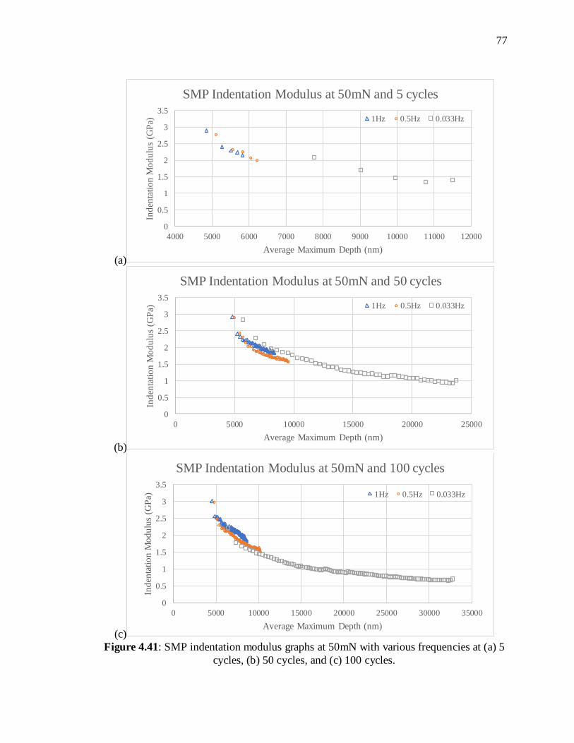
77
(a)
(b)
(c) Figure 4.41: SMP indentation modulus graphs at 50mN with various frequencies at (a) 5
cycles, (b) 50 cycles, and (c) 100 cycles.
0
0.5
1
1.5
2
2.5
3
3.5
4000 5000 6000 7000 8000 9000 10000 11000 12000
Ind
enta
tio
n M
od
ulu
s (G
Pa)
Average Maximum Depth (nm)
SMP Indentation Modulus at 50mN and 5 cycles
1Hz 0.5Hz 0.033Hz
0
0.5
1
1.5
2
2.5
3
3.5
0 5000 10000 15000 20000 25000
Ind
enta
tio
n M
od
ulu
s (G
Pa)
Average Maximum Depth (nm)
SMP Indentation Modulus at 50mN and 50 cycles
1Hz 0.5Hz 0.033Hz
0
0.5
1
1.5
2
2.5
3
3.5
0 5000 10000 15000 20000 25000 30000 35000
Ind
enta
tio
n M
od
ulu
s (G
Pa)
Average Maximum Depth (nm)
SMP Indentation Modulus at 50mN and 100 cycles
1Hz 0.5Hz 0.033Hz

78
(a)
(b)
(c) Figure 4.42: SMP indentation modulus graphs at 50mN with various cycles at (a) 1Hz,
(b) 0.5Hz, and (c) 0.033Hz.
1.5
1.7
1.9
2.1
2.3
2.5
2.7
2.9
3.1
4000 5000 6000 7000 8000 9000
Ind
enta
tio
n M
od
ulu
s (G
Pa)
Average Maximum Depth (nm)
SMP Indentation Modulus at 50mN and 1Hz
5 cycles 50 cycles 100 cycles
1
1.5
2
2.5
3
3.5
4000 5000 6000 7000 8000 9000 10000 11000
Ind
enta
tio
n M
od
ulu
s (G
Pa)
Average Maximum Depth (nm)
SMP Indentation Modulus at 50mN and 0.5Hz
5 cycles 50 cycles 100 cycles
0
0.5
1
1.5
2
2.5
3
0 5000 10000 15000 20000 25000 30000 35000
Ind
enta
tio
n M
od
ulu
s (G
Pa)
Average Maximum Depth (nm)
SMP Indentation Modulus at 50mN and 0.033Hz
5 cycles 50 cycles 100 cycles
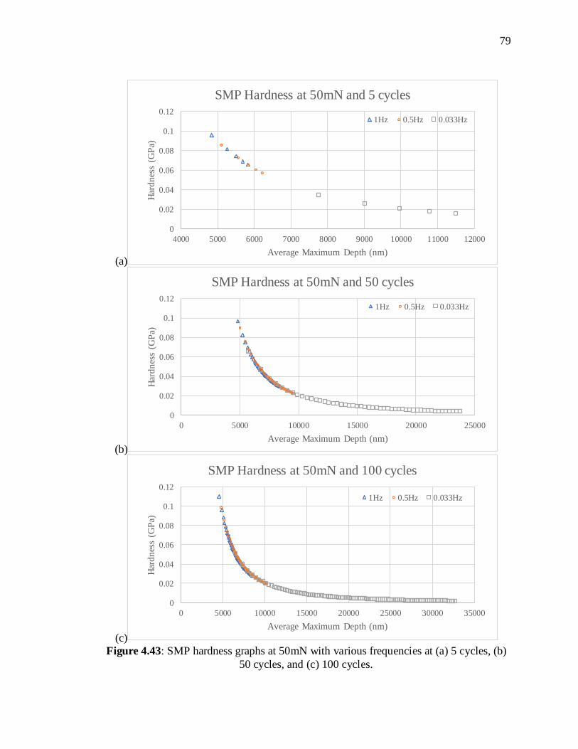
79
(a)
(b)
(c) Figure 4.43: SMP hardness graphs at 50mN with various frequencies at (a) 5 cycles, (b)
50 cycles, and (c) 100 cycles.
0
0.02
0.04
0.06
0.08
0.1
0.12
4000 5000 6000 7000 8000 9000 10000 11000 12000
Har
dn
ess
(GP
a)
Average Maximum Depth (nm)
SMP Hardness at 50mN and 5 cycles
1Hz 0.5Hz 0.033Hz
0
0.02
0.04
0.06
0.08
0.1
0.12
0 5000 10000 15000 20000 25000
Har
dn
ess
(GP
a)
Average Maximum Depth (nm)
SMP Hardness at 50mN and 50 cycles
1Hz 0.5Hz 0.033Hz
0
0.02
0.04
0.06
0.08
0.1
0.12
0 5000 10000 15000 20000 25000 30000 35000
Har
dn
ess
(GP
a)
Average Maximum Depth (nm)
SMP Hardness at 50mN and 100 cycles
1Hz 0.5Hz 0.033Hz

80
(a)
(b)
(c) Figure 4.44: SMP hardness graphs at 50mN with various frequencies at (a) 1Hz, (b)
0.5Hz, and (c) 0.033Hz.
0.02
0.03
0.04
0.05
0.06
0.07
0.08
0.09
0.1
0.11
0.12
4000 5000 6000 7000 8000 9000
Har
dn
ess
(GP
a)
Average Maximum Depth (nm)
SMP Hardness at 50mN and 1Hz
5 cycles 50 cycles 100 cycles
0
0.02
0.04
0.06
0.08
0.1
0.12
4000 5000 6000 7000 8000 9000 10000 11000
Har
dn
ess
(GP
a)
Average Maximum Depth (nm)
SMP Hardness at 50mN and 0.5Hz
5 cycles 50 cycles 100 cycles
0
0.01
0.02
0.03
0.04
0.05
0.06
0.07
0 5000 10000 15000 20000 25000 30000 35000
Har
dn
ess
(GP
a)
Average Maximum Depth (nm)
SMP Hardness at 50mN and 0.033Hz
5 cycles 50 cycles 100 cycles
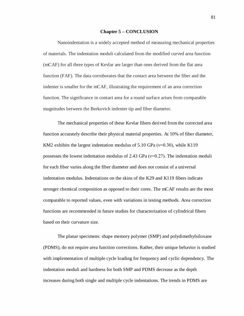
81
Chapter 5 – CONCLUSION
Nanoindentation is a widely accepted method of measuring mechanical properties
of materials. The indentation moduli calculated from the modified curved area function
(mCAF) for all three types of Kevlar are larger than ones derived from the flat area
function (FAF). The data corroborates that the contact area between the fiber and the
indenter is smaller for the mCAF, illustrating the requirement of an area correction
function. The significance in contact area for a round surface arises from comparable
magnitudes between the Berkovich indenter tip and fiber diameter.
The mechanical properties of these Kevlar fibers derived from the corrected area
function accurately describe their physical material properties. At 10% of fiber diameter,
KM2 exhibits the largest indentation modulus of 5.10 GPa (ν=0.30), while K119
possesses the lowest indentation modulus of 2.43 GPa (ν=0.27). The indentation moduli
for each fiber varies along the fiber diameter and does not consist of a universal
indentation modulus. Indentations on the skins of the K29 and K119 fibers indicate
stronger chemical composition as opposed to their cores. The mCAF results are the most
comparable to reported values, even with variations in testing methods. Area correction
functions are recommended in future studies for characterization of cylindrical fibers
based on their curvature size.
The planar specimens: shape memory polymer (SMP) and polydimethylsiloxane
(PDMS), do not require area function corrections. Rather, their unique behavior is studied
with implementation of multiple cycle loading for frequency and cyclic dependency. The
indentation moduli and hardness for both SMP and PDMS decrease as the depth
increases during both single and multiple cycle indentations. The trends in PDMS are
82
linear for 5 and 50 cycles, whereas 100 cycle tests for mechanical properties favor power
law curve fits. Linearity is displayed in PDMS at 1 and 0.5Hz controlled tests, while
0.033Hz tests follow power law curve fits. All three cycles and frequencies exhibit power
law trends in SMP specimens. The mechanical properties of PDMS measured in the
present study comply with reported literature, further affirming the precisions of
indentation results. When the loads are increased for indentation experiments on both
materials, the indentation moduli decrease as the maximum depth increases. A similar
pattern is also evident for the hardness of both materials. Typically, the depth increases
drastically at lower frequencies, indicating creep behavior. The tests from single cycle
indentation validate with ones from multiple cycle loading, confirming the accuracy of
data yielded from the two processes.
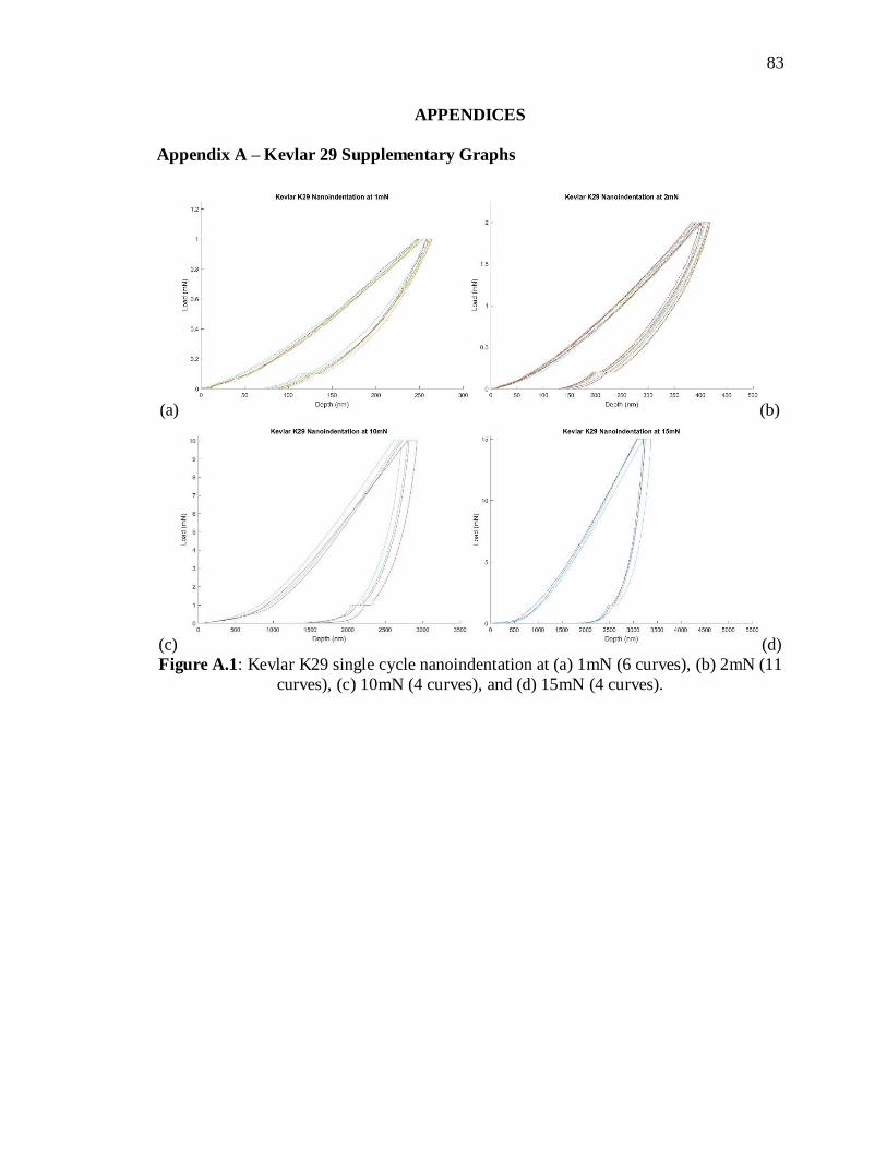
83
APPENDICES
Appendix A – Kevlar 29 Supplementary Graphs
(a) (b)
(c) (d)
Figure A.1: Kevlar K29 single cycle nanoindentation at (a) 1mN (6 curves), (b) 2mN (11
curves), (c) 10mN (4 curves), and (d) 15mN (4 curves).
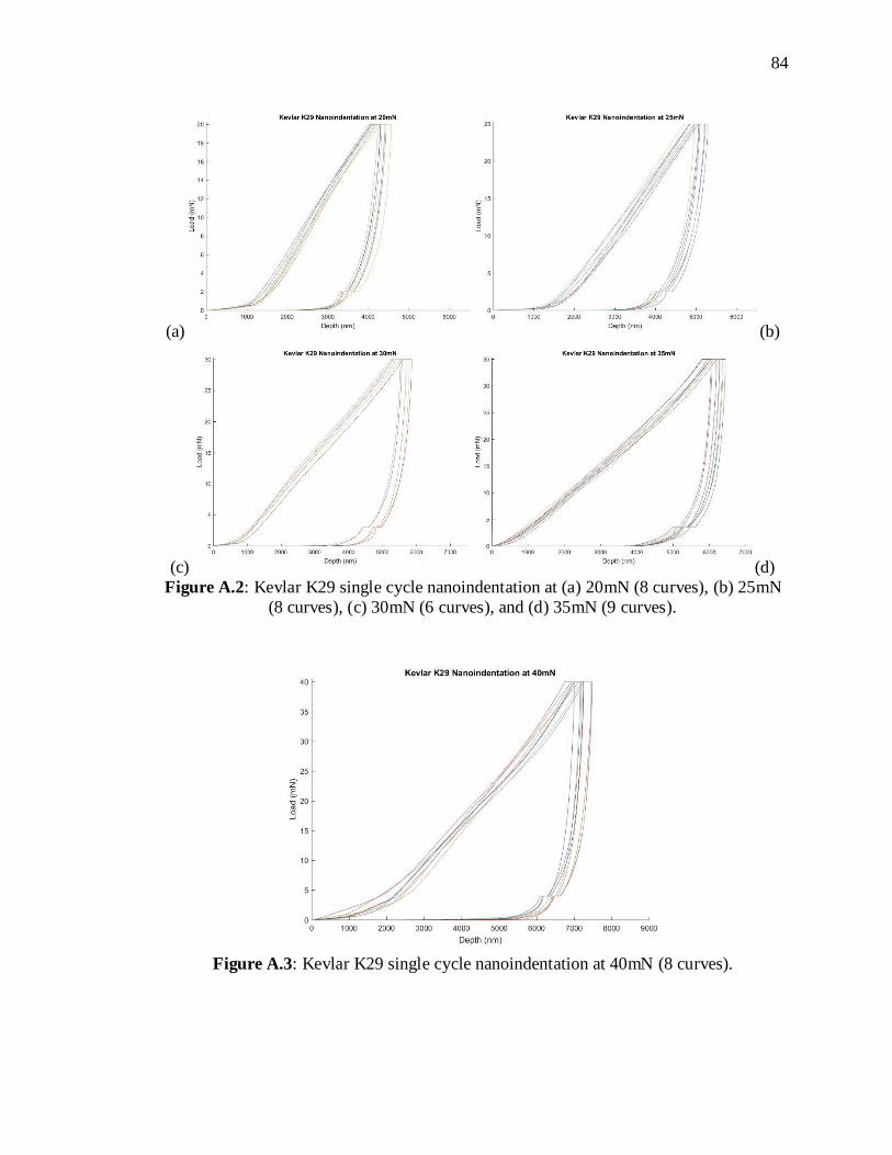
84
(a) (b)
(c) (d)
Figure A.2: Kevlar K29 single cycle nanoindentation at (a) 20mN (8 curves), (b) 25mN
(8 curves), (c) 30mN (6 curves), and (d) 35mN (9 curves).
Figure A.3: Kevlar K29 single cycle nanoindentation at 40mN (8 curves).

85
Appendix B – Kevlar KM2 Supplementary Graphs
(a) (b)
(c)
Figure B.1: Kevlar KM2 single cycle nanoindentation at (a) 1mN (3 curves), (b) 2mN (4
curves), and (c) 3mN (6 curves).
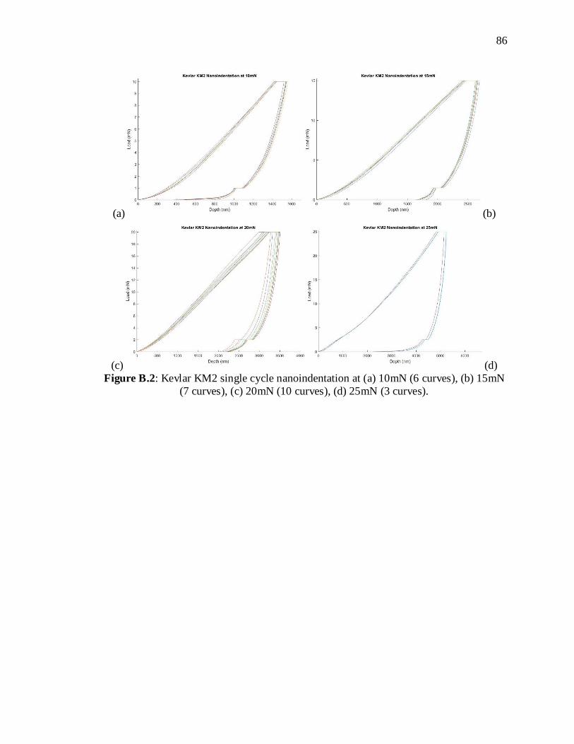
86
(a) (b)
(c) (d)
Figure B.2: Kevlar KM2 single cycle nanoindentation at (a) 10mN (6 curves), (b) 15mN
(7 curves), (c) 20mN (10 curves), (d) 25mN (3 curves).
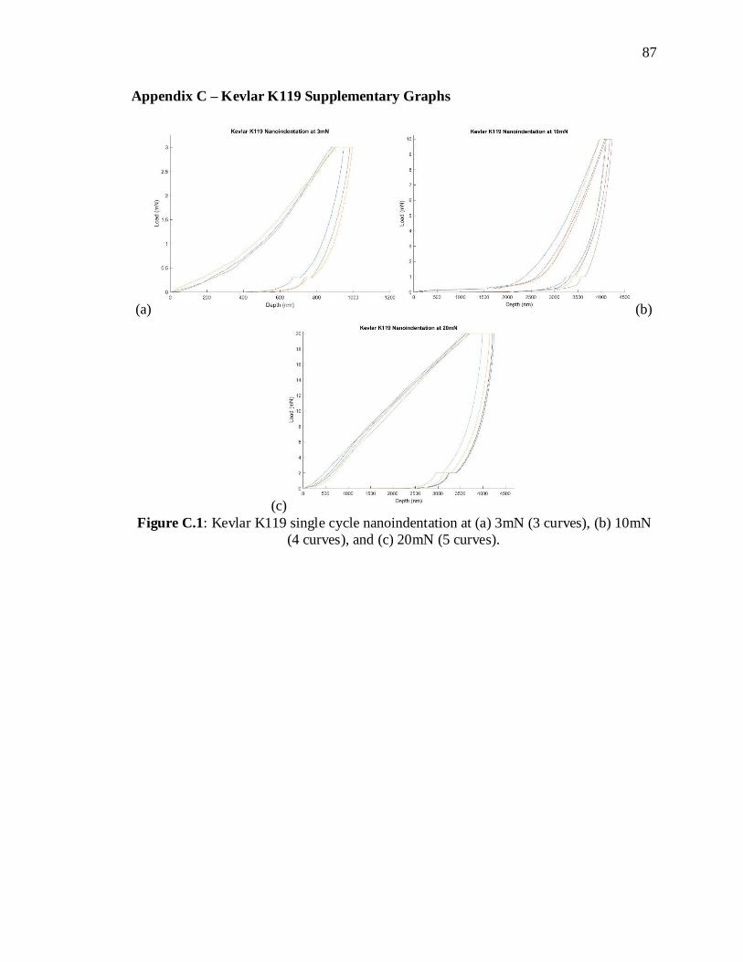
87
Appendix C – Kevlar K119 Supplementary Graphs
(a) (b)
(c)
Figure C.1: Kevlar K119 single cycle nanoindentation at (a) 3mN (3 curves), (b) 10mN
(4 curves), and (c) 20mN (5 curves).
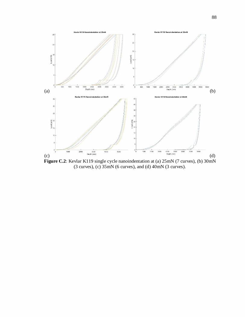
88
(a) (b)
(c) (d)
Figure C.2: Kevlar K119 single cycle nanoindentation at (a) 25mN (7 curves), (b) 30mN
(3 curves), (c) 35mN (6 curves), and (d) 40mN (3 curves).
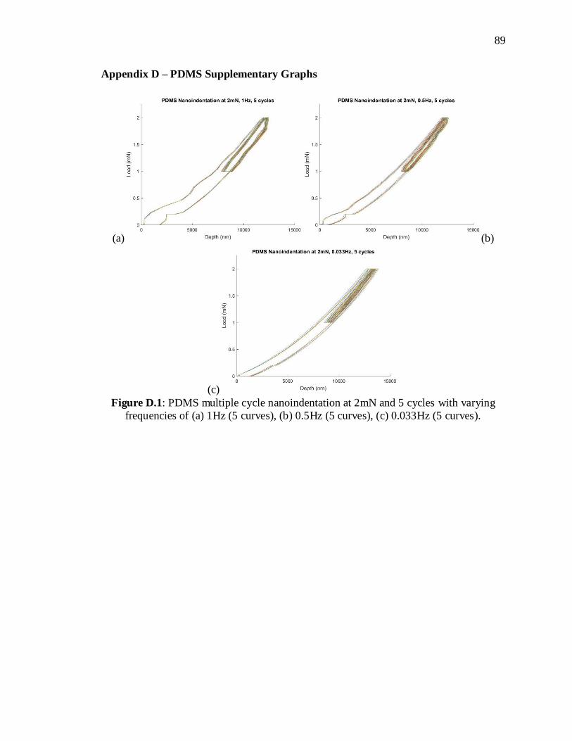
89
Appendix D – PDMS Supplementary Graphs
(a) (b)
(c)
Figure D.1: PDMS multiple cycle nanoindentation at 2mN and 5 cycles with varying
frequencies of (a) 1Hz (5 curves), (b) 0.5Hz (5 curves), (c) 0.033Hz (5 curves).
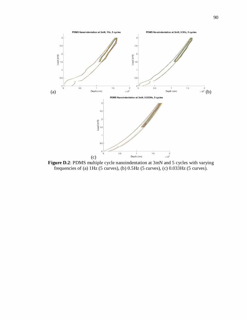
90
(a) (b)
(c)
Figure D.2: PDMS multiple cycle nanoindentation at 3mN and 5 cycles with varying
frequencies of (a) 1Hz (5 curves), (b) 0.5Hz (5 curves), (c) 0.033Hz (5 curves).

91
(a) (b)
(c)
Figure D.3: PDMS multiple cycle nanoindentation at 1mN and 50 cycles with varying
frequencies of (a) 1Hz (5 curves), (b) 0.5Hz (5 curves), (c) 0.033Hz (5 curves).
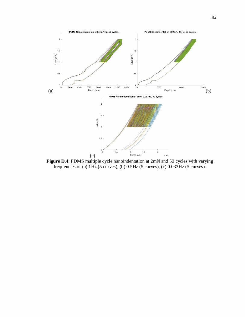
92
(a) (b)
(c)
Figure D.4: PDMS multiple cycle nanoindentation at 2mN and 50 cycles with varying
frequencies of (a) 1Hz (5 curves), (b) 0.5Hz (5 curves), (c) 0.033Hz (5 curves).
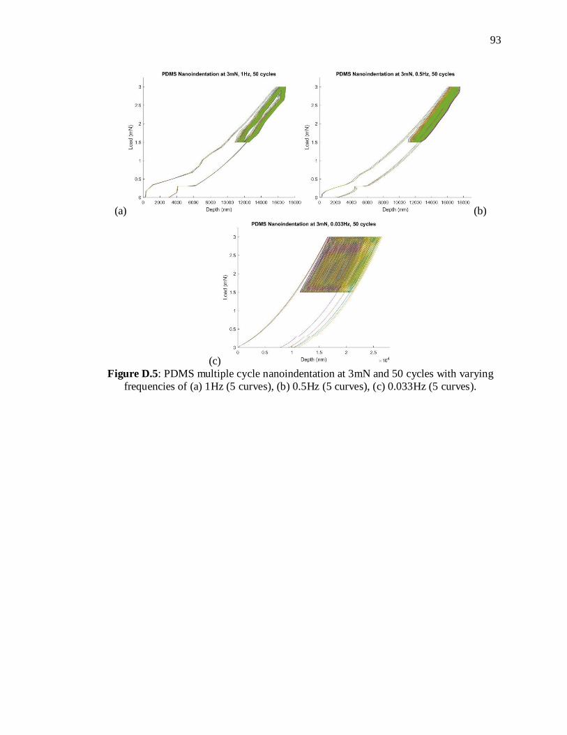
93
(a) (b)
(c)
Figure D.5: PDMS multiple cycle nanoindentation at 3mN and 50 cycles with varying
frequencies of (a) 1Hz (5 curves), (b) 0.5Hz (5 curves), (c) 0.033Hz (5 curves).
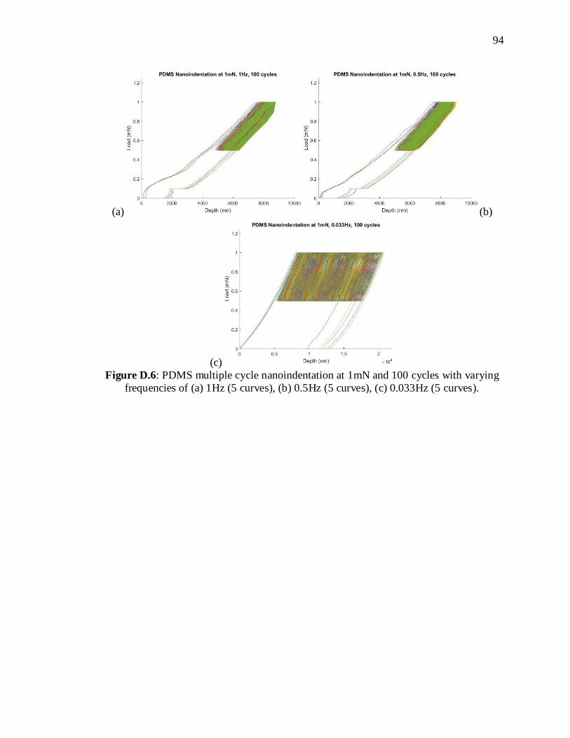
94
(a) (b)
(c)
Figure D.6: PDMS multiple cycle nanoindentation at 1mN and 100 cycles with varying
frequencies of (a) 1Hz (5 curves), (b) 0.5Hz (5 curves), (c) 0.033Hz (5 curves).
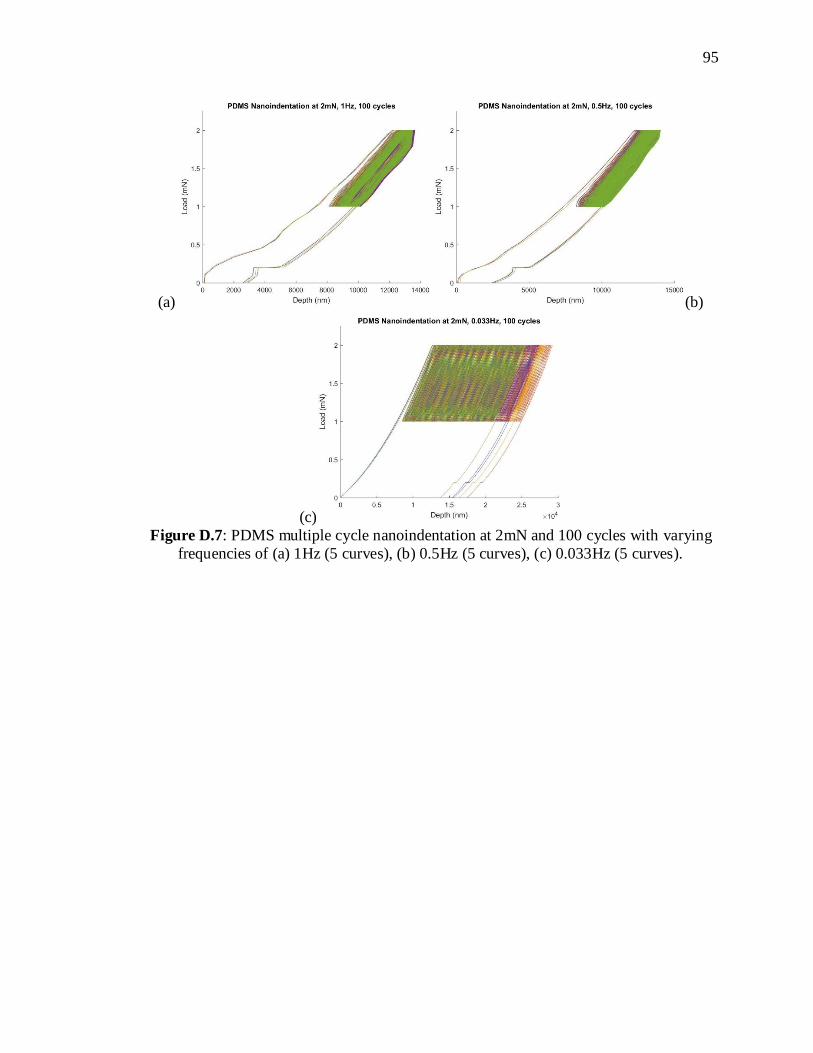
95
(a) (b)
(c)
Figure D.7: PDMS multiple cycle nanoindentation at 2mN and 100 cycles with varying
frequencies of (a) 1Hz (5 curves), (b) 0.5Hz (5 curves), (c) 0.033Hz (5 curves).
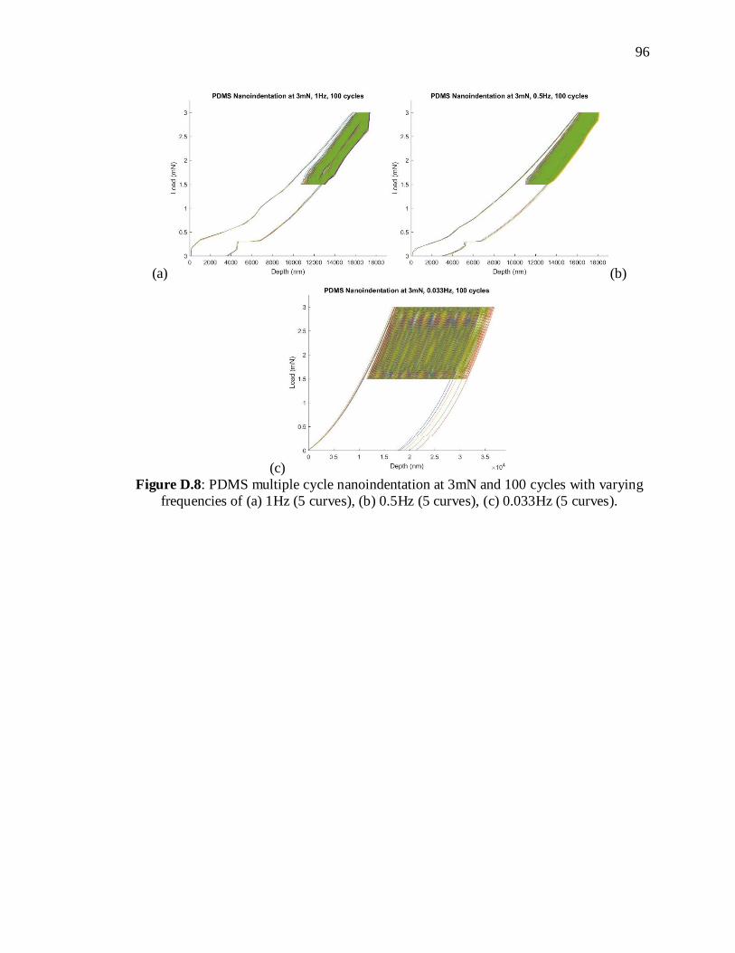
96
(a) (b)
(c)
Figure D.8: PDMS multiple cycle nanoindentation at 3mN and 100 cycles with varying
frequencies of (a) 1Hz (5 curves), (b) 0.5Hz (5 curves), (c) 0.033Hz (5 curves).
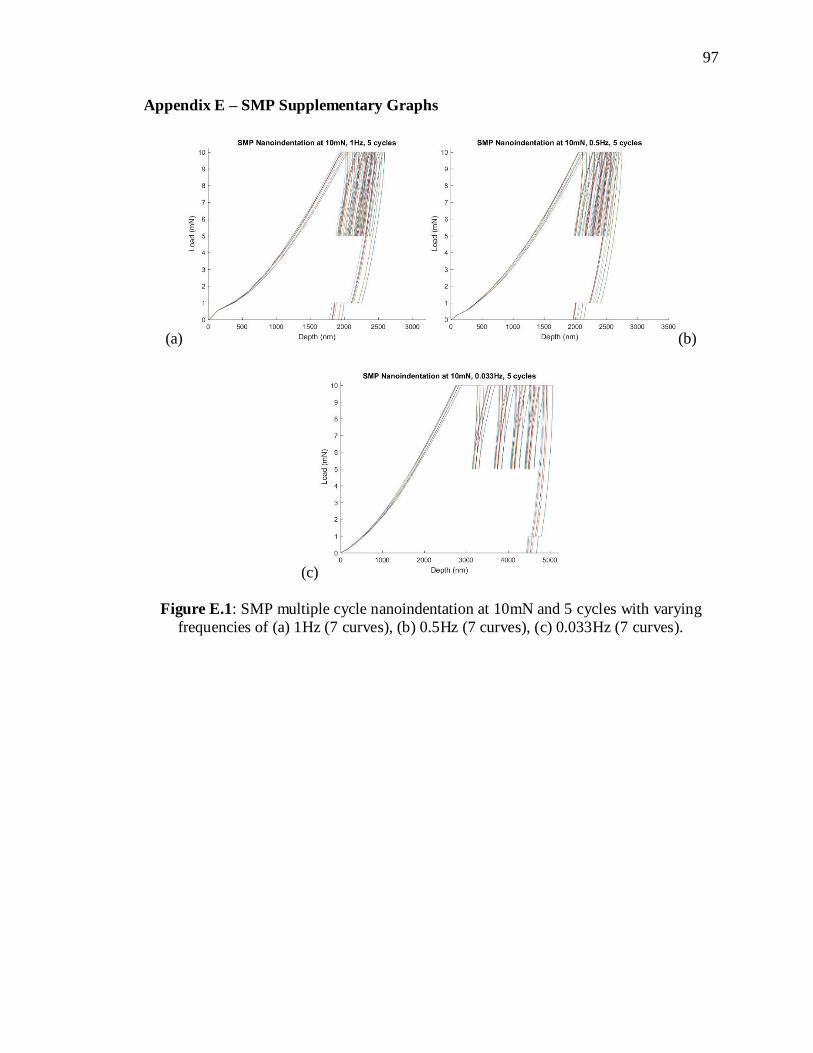
97
Appendix E – SMP Supplementary Graphs
(a) (b)
(c)
Figure E.1: SMP multiple cycle nanoindentation at 10mN and 5 cycles with varying
frequencies of (a) 1Hz (7 curves), (b) 0.5Hz (7 curves), (c) 0.033Hz (7 curves).
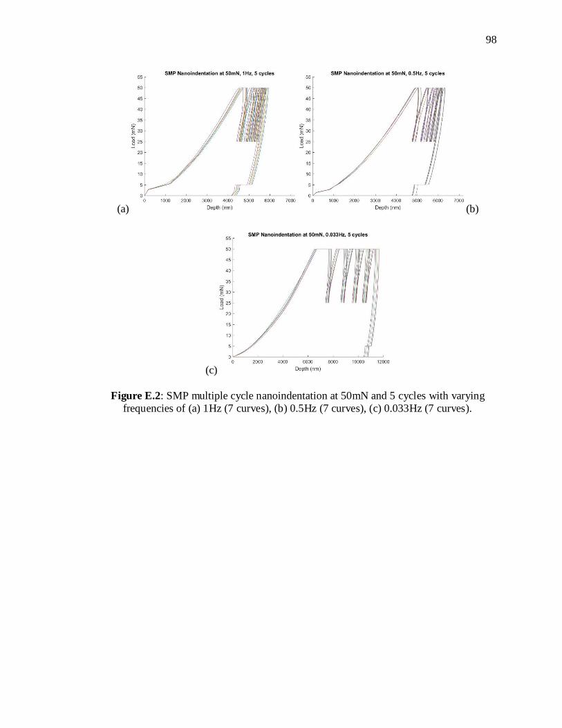
98
(a) (b)
(c)
Figure E.2: SMP multiple cycle nanoindentation at 50mN and 5 cycles with varying
frequencies of (a) 1Hz (7 curves), (b) 0.5Hz (7 curves), (c) 0.033Hz (7 curves).
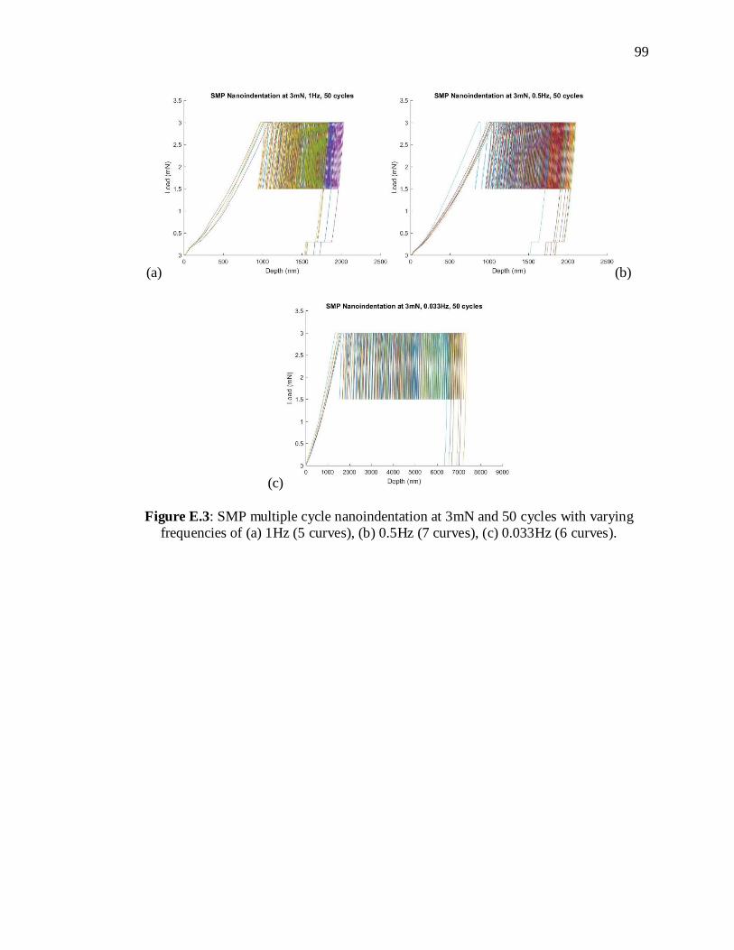
99
(a) (b)
(c)
Figure E.3: SMP multiple cycle nanoindentation at 3mN and 50 cycles with varying
frequencies of (a) 1Hz (5 curves), (b) 0.5Hz (7 curves), (c) 0.033Hz (6 curves).
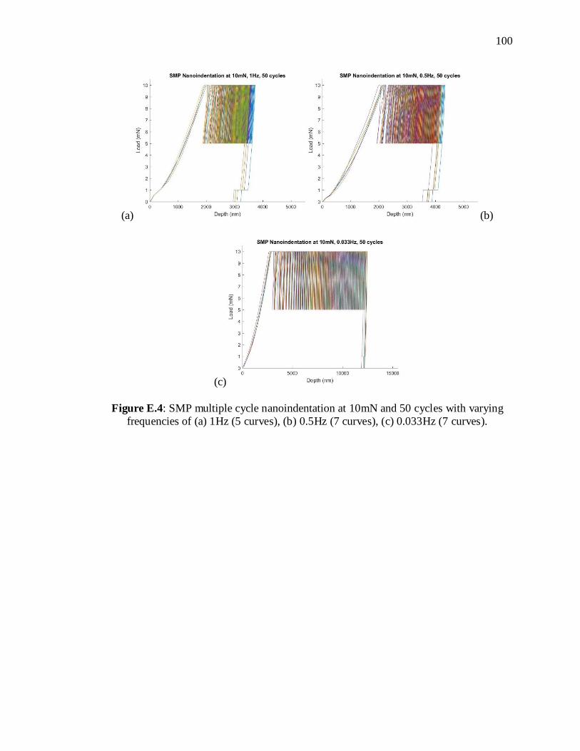
100
(a) (b)
(c)
Figure E.4: SMP multiple cycle nanoindentation at 10mN and 50 cycles with varying
frequencies of (a) 1Hz (5 curves), (b) 0.5Hz (7 curves), (c) 0.033Hz (7 curves).

101
(a) (b)
(c)
Figure E.5: SMP multiple cycle nanoindentation at 50mN and 50 cycles with varying
frequencies of (a) 1Hz (7 curves), (b) 0.5Hz (5 curves), (c) 0.033Hz (5 curves).
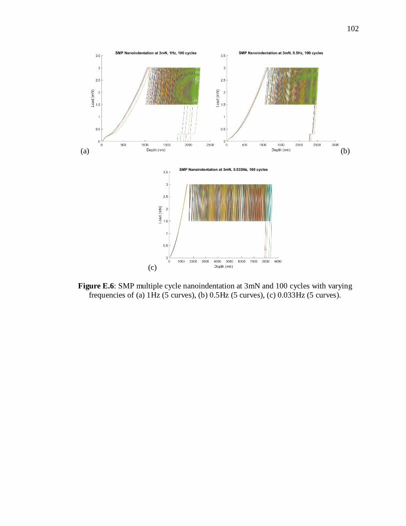
102
(a) (b)
(c)
Figure E.6: SMP multiple cycle nanoindentation at 3mN and 100 cycles with varying
frequencies of (a) 1Hz (5 curves), (b) 0.5Hz (5 curves), (c) 0.033Hz (5 curves).
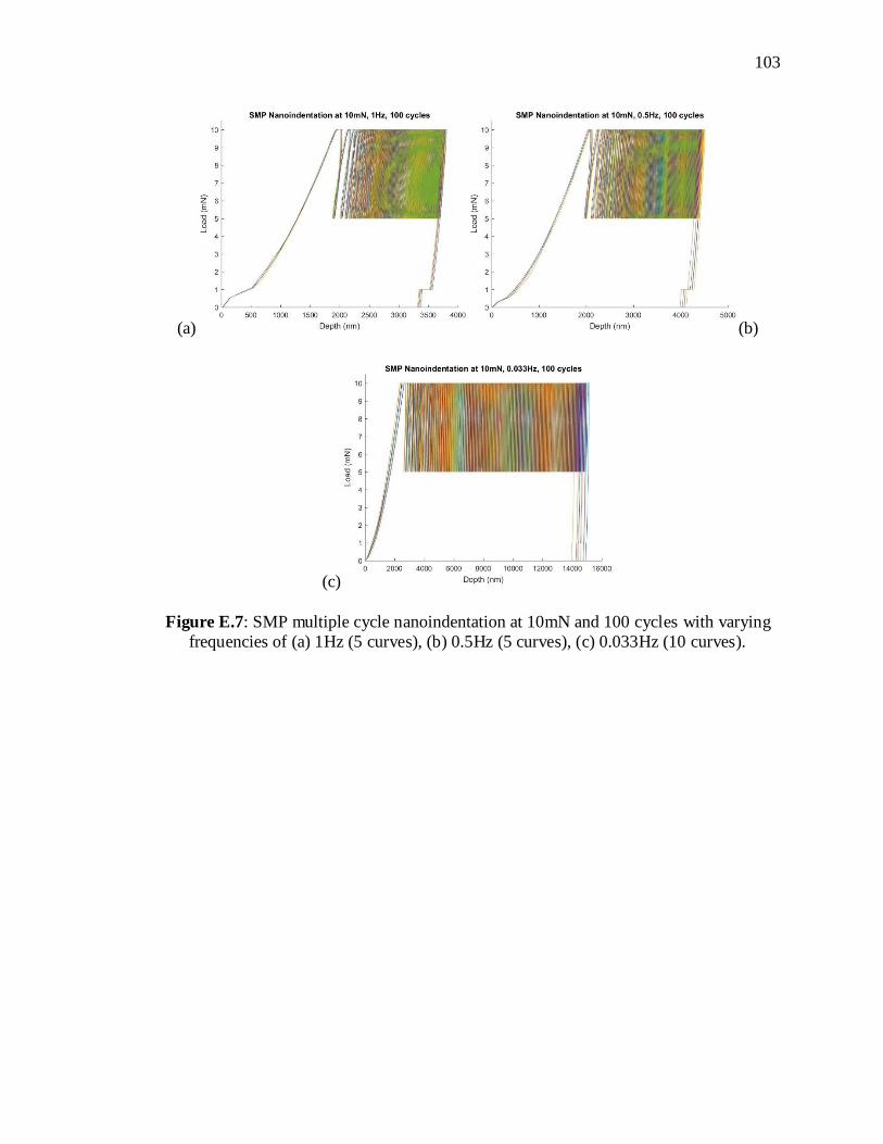
103
(a) (b)
(c)
Figure E.7: SMP multiple cycle nanoindentation at 10mN and 100 cycles with varying
frequencies of (a) 1Hz (5 curves), (b) 0.5Hz (5 curves), (c) 0.033Hz (10 curves).

104
(a) (b)
(c)
Figure E.8: SMP multiple cycle nanoindentation at 50mN and 100 cycles with varying
frequencies of (a) 1Hz (5 curves), (b) 0.5Hz (5 curves), (c) 0.033Hz (10 curves).
105
REFERENCES
[1] Quintanilla, J. “Microstructure and Properties of Random Heterogeneous Materials: a
Review of Theoretical Results.” Polymer Engineering and Science Vol. 39 No. 3 (1999):
pp. 559-585.
[2] Kabir, Reashad Bin and Ferdous, Nasrin. “Kevlar-The Super Tough Fiber.”
International Journal of Textile Science Vol. 1 No. 6 (2012): pp. 78-83. DOI
10.5923/j.textile.20120106.04.
[3] Carmichael, Neil. “Linear Polydimethylsiloxanes CAS No. 63148-62-9 (Second
Edition).” Technical Report No. JACC 55. European Centre for Ecotoxicology and
Toxicology of Chemicals, Brussels, Belgium. 2011.
[4] Lin, Chien-Hong, Yeh, Yi-Hsing, Lin, Wen-Ching, and Yang, Ming-Chien. “Novel
silicone hydrogel based on PDMS and PEGMA for contact lens application.” Colloids
and Surfaces B: Biointerfaces Vol. 123 (2014): pp. 986-994. DOI
10.1016/j.colsurfb.2014.10.053.
[5] Lotters, J.C., Olthuis, W., Veltink P.H., and Bergveld, P. “The mechanical properties
of the rubber elastic polymer polydimethylsiloxane for sensor applications.” J.
Micromech. Microeng. Vol. 7 No. 3 (1997): pp. 145-147. DOI 10.1088/0960-
1317/7/3/017.
[6] Mather, Patrick T., Luo, Xiaofan, and Rousseau, Ingrid A. “Shape Memory Polymer
Research.” Annu. Rev. Mater. Res. Vol. 39 (2009): pp. 445-471. DOI 10.1146/annurev-
matsci-082908-145419.
[7] Ratna, Debdatta and Karger-Kocsis, J. “Recent advances in shape memory polymers
and composites: a review.” J Mater Sci Vol. 43 No. 1 (2008): pp. 254-269. DOI
10.1007/s10853-007-2176-7.
[8] Sokolowski, Witold, Metcalfe, Annick, Hayashi, Shunichi, Yahia, L’Hocine, and
Raymond, Jean. “Medical applications of shape memory polymers.” Biomed. Mater. Vol.
2 No. 1 (2007): pp. S23-S27. DOI 10.1088/1748-6041/2/1/S04.
[9] Ge, Qi, Sakhaei, Amir Hosein, Lee, Howon, Dunn, Conner K., Fang, Nicholas X., and
Dunn, Martin L. “Multimaterial 4D Printing with Tailorable Shape Memory Polymers.”
Scientific Reports Vol. 6 No. 31110 (2016): pp. 1-11. DOI 10.1038/srep31110.
[10] Yang, Chen, Boorugu, Manish, Dopp, Andrew, Ren, Jie, Martin, Raymond, Han,
Daehoon, Choi, Wonjoon, and Lee, Howon. “4D Printing Reconfigurable, Deployable
and Mechanically Tunable Metamaterials.” Mater. Horiz. (2019): DOI
10.1039/C9MH00302A.
106
[11] Bhushan, Bharat. “Depth-sensing nanoindentation measurement techniques and
applications.” Microsyst Technol Vol. 23 No. 5 (2017): pp. 1595-1649. DOI
10.1007/s00542-017-3372-2.
[12] Wierenga, P.E. and Franken, A.J.J. “Ultramicroindentation apparatus for the
mechanical characterization of thin films.” Journal of Applied Physics Vol. 55 No. 12
(1984): pp. 4244-4247. DOI 10.1063/1.333026.
[13] Turla, Prashanth. “Updated Area Function Analysis for Nano Indentation of Micro
Fibers.” MS Thesis. Rutgers University, New Brunswick, NJ. 2017. DOI
10.7282/T3S185N6.
[14] McAllister, Quinn P., Gillespie, John W. Jr. and VanLandingham, Mark R. “The
sub-micron scale energy dissipative deformation mechanisms of Kevlar fibrils.” J Mater
Sci Vol. 48 No. 18 (2013): pp. 6245-6261. DOI 10.1007/s10853-013-7422-6.
[15] McAllister, Quinn P. and Gillespie, John W. Jr. “Evaluation of the three-dimensional
properties of Kevlar across length scales.” J. Mater. Res. Vol. 27 No. 14 (2012): pp.
1824-1837. DOI 10.1557/jmr.2012.80.
[16] Cole, Daniel P. and Strawhecker, Kenneth E. “An improved instrumented
indentation technique for single microfibers.” J. Mater. Res. Vol. 29 No. 9 (2014): pp.
1104-1112. DOI 10.1557/jmr.2014.83.
[17] Bencomo-Cisneros, J.A., Tejeda-Ochoa, A., García-Estrada, J.A., Herrera-Ramírez,
C.A., Hurtado-Macías, A., Martínez-Sánchez, R., and Herrera-Ramírez, J.M.
“Characterization of Kevlar-29 fibers by tensile tests and nanoindentation.” Journal of
Alloys and Compounds Vol. 536 No. 1 (2012): pp. S456-S459. DOI
10.1016/j.jallcom.2011.11.031.
[18] Kawabata, S. “Measurement of the Transverse Mechanical Properties of High-
performance Fibres.” J. Text. Inst. Vol. 81 No. 4 (1990): pp. 432-447.
[19] Wollbrett-Blitz, Judith, Joannès, Sébastien, Bruant, Rémi, Le Clerc, Christophe, De
La Osa, Marc Romero, Bunsell, Anthony, and Marcellan, Alba. “Multiaxial Mechanical
Behavior of Aramid Fibers and Identification of Skin/Core Structure from Single Fiber
Transverse Compression Testing.” Journal of Polymer Science, Part B: Polymer Physics
Vol. 54 No. 3 (2015): pp. 374-384. DOI 10.1002/polb.23763.
[20] Fisher-Cripps, Anthony C. “The sharpness of a Berkovich indenter.” J. Mater. Res.
Vol. 25 No. 5 (2010): pp. 927-934. DOI 10.1557/JMR.2010.0111.

107
[21] Carillo, Fernando, Gupta, Shikha, Balooch, Mehdi, Marshall, Sally J., Marshall,
Grayson W., Pruitt, Lisa, and Puttlitz, Christian M. “Nanoindentation of
polydimethylsiloxane elastomers: Effect of crosslinking, work of adhesion, and fluid
environment on elastic modulus.” J. Mater. Res. Vol. 20 No. 10 (2005): pp. 2820-2830.
DOI 10.1557/JMR.2005.0354.
[22] Maji, Debashis and Das, Soumen. “Atomic force microscopy and nanoindentation
investigation of polydimethylsiloxane elastomeric substrate compliancy for various
sputtered thin film morphologies.” J Biomed Mater Res A Vol. 106 No. 3 (2017): pp.
725-737. DOI 10.1002/jbm.a.36283.
[23] Saha, Ranjana and Nix, William D. “Effects of the substrate on the determination of
thin film mechanical properties by nanoindentation.” Acta Materialia Vol. 50 No. 1
(2002): pp. 23-38. DOI 10.1016/S1359-6454(01)00328-7.
[24] Chudoba, T. and Richter, F. “Investigation of creep behaviour under load during
indentation experiments and its influence on hardness and modulus results.” Surface and
Coatings Technology Vol. 148 No. 2-3 (2001): pp. 191-198. DOI 10.1016/S0257-
8972(01)01340-8.
[25] Rho, Jae-Young and Pharr, G.M. “Effects of drying on the mechanical properties of
bovine femur measured by nanoindentation.” Journal of Materials Science Vol. 10 No. 8
(1999): pp. 485-488.
[26] Oliver, W.C. and Pharr, G.M. “An improved technique for determining hardness and
elastic modulus using load and displacement sensing indentation experiments.” J. Mater.
Res. Vol. 7 No. 6 (1992): pp. 1564-1583. DOI 10.1557/JMR.1992.1564.
[27] Doerner, M.F. and Nix, W.D. “A method for interpreting the data from depth-
sensing indentation instruments.” J. Mater. Res. Vol. 1 No. 4 (1986): pp. 601-609. DOI
10.1557/JMR.1986.0601.
[28] Schwarzer, N. “The extended Hertzian theory and its uses in analyzing indentation
experiments.” Philosophical Magazine Vol. 86 No. 33-35 (2006): pp. 5179-5197. DOI
10.1080/14786430600690507.
[29] Vlassak, Joost J. and Nix, W. D. “Measuring the elastic properties of anisotropic
materials by means of indentation experiments.” J. Mech. Phys. Solids Vol. 42 No. 8
(1994): pp. 1223-1245. DOI 10.1016/0022-5096(94)90033-7.
[30] Nano Test User Manual. Micro Materials Excellence in Nano-mechanics. (2015)
[31] Alisafaei, F. and Han, Chung-Souk. “Indentation Depth Dependent Mechanical
Behavior in Polymers.” Advances in Condensed Matter Physics Vol. 2015 No. 391579
(2015) pp. 1-20. DOI 10.1155/2015/391579.
108
[32] Hardiman, M., Vaughan, T.J., and McCarthy, C.T. “The effects of pile-up,
viscoelasticity and hydrostatic stress on polymer matrix nanoindentation.” Polymer
Testing Vol. 52 (2016): pp. 157-166. DOI 10.1016/j.polymertesting.2016.04.003.
[33] Han, Chung-Souk. “Indentation Size Effect in Polymers.” Advances in Materials
Science Research Vol. 10 No. 15 (2011): pp. 393-413.
[34] Briscoe, B.J., Fiori, L., and Pelillo, E. “Nano-indentation of polymeric surfaces.” J.
Phys. D: Appl. Phys. Vol. 31 No. 19 (1998): pp. 2395-2405. DOI 10.1088/0022-
3727/31/19/006.
[35] Bandyopadhyay, P.P., Chicot, D., Kumar, C.S., Decoopman, X., and Lesage, J.
“Influence of sinking-in and piling-up on the mechanical properties determination by
indentation: A case study on rolled and DMLS stainless steel.” Materials Science &
Engineering A Vol. 576 (2013): pp. 126-133. DOI 10.1016/j.msea.2013.03.081.
[36] Cheng, Yang-Tse and Cheng, Che-Min. “Scaling approach to conical indentation in
elastic-plastic solids with work hardening.” Journal of Applied Physics Vol. 84 No. 3
(1998): pp. 1284-1291. DOI 10.1063/1.368196.
[37] Qu, Zhaoliang, Pei, Yongmao, He, Rujie, and Fang, Daining. “Investigation of Pile-
Up Behavior for Thermal Barrier Coatings Under Elevated-Temperature Indentation.”
Journal of Applied Mechanics Vol. 83 No. 4 (2016): pp. 1-6. DOI 10.1115/1.4032467.
[38] Swadener, J.G., George, E.P., and Pharr G.M. “The correlation of the indentation
size effect measured with indenters of various shapes.” Journal of the Mechanics and
Physics of Solids Vol. 50 No. 4 (2002): pp. 681-694. DOI 10.1016/S0022-
5096(01)00103-X.
[39] Fischer-Cripps, Anthony C. “Chapter 2 Nanoindentation Testing.” Nanoindentation.
Springer-Verlag, New York (2011): pp. 21-37.
[40] TI 750 Ubi User Manual, Hysitron. Revision 9.2.0311.
[41] Sakharova, N.A, Fernandes, J.V., Antunes, J.M., and Oliveira, M.C. “Comparison
between Berkovich, Vickers, and conical indentation tests: A three-dimensional
numerical simulation study.” International Journal of Solids and Structures Vol. 46 No.
5 (2009): pp. 1095-1104. DOI 10.1016/j.ijsolstr.2008.10.032.
[42] Raju, Hermise and Pelegri, Assimina A. “Experimental Investigation of Transverse
Mechanical Properties of High-Performance Kevlar KM2 Single Fiber.” ASME 2017
International Mechanical Engineering Congress and Exposition. IMECE2017-71724: pp.
V014T11A045. Tampa, Florida, November 3-9, 2017. DOI 10.1115/IMECE2017-71724.
109
[43] Wang, Zhixin, Volinsky, Alex A., Gallant, Nathan D. “Nanoindentation Study of
Polydimethylsiloxane Elastic Modulus Using Berkovich and Flat Punch Tips.” Journal of
Applied Polymer Science Vol. 132 No. 5 (2014): pp. 1-7. DOI 10.1002/app.41384.
[44] Safranski, David L. and Gall, Ken. “Effect of chemical structure and crosslinking
density on the thermo-mechanical properties and toughness of (meth)acrylate shape
memory polymer networks.” Polymer Vol. 49 No. 20 (2008): pp. 4446-4455. DOI
10.1016/j.polymer.2008.07.060.
[45] Wang, J.S., Zheng, X.J., Zheng, H., Zhu, Z., and Song, S.T. “Evaluation of the
substrate effect on indentation behavior of film/substrate system.” Applied Surface
Science Vol. 256 No. 20 (2010): pp. 5998-6002. DOI 10.1016/j.apsusc.2010.03.108.
[46] Jiang, Wu-Gui, Feng, Xi-Qiao, and Su, Jian-Jun. “Effect of surface roughness on
nanoindentation test of thin films.” Engineering Fracture Mechanics Vol. 75 No. 17
(2008): pp. 4965-4972. DOI 10.1016/j.engfracmech.2008.06.016.
[47] Jiroušek, Ondřej, Kytyr, Dan, Zlámal, Petr, Doktor, Tomáš, Šepitka, Josef, and
Lukeš, Jaroslav. “Use of Modulus Mapping Technique to Investigate Cross-sectional
Material Properties of Extracted Single Human Trabeculae.” Chem. Listy Vol. 106
(2012): pp. 442-445.
[48] Cheng, Ming, Chen, Weinong, and Weerasooriya, Tusit. “Experimental
investigation of the transverse mechanical properties of a single Kevlar® KM2 fiber.”
International Journal of Solids and Structures Vol. 41 No. 22-23 (2004): pp. 6215-6232.
DOI 10.1016/j.ijsolstr.2004.05.016.
[49] Muhammed, Luay and Ismaeel, Luay. “Effect of Shear Modular Ratio (G F /G M )
and Transverse Shear Modulus on the Twisting Strength of a Fiber- Reinforced
Composite Rod.” The Iraqi Journal for Mechanical and Material Engineering Vol. 13
No. 1 (2013): pp. 129-143.
[50] Şahin, Korhan, Clawson, Jan Kenneth, Singletary, James, Horner, Suzanne, Zheng,
James, Pelegri, Assimina, and Chasiotis, Ioannis. “Limiting role of crystalline domain
orientation on the modulus and strength of aramid fibers.” Polymer Vol. 140 (2018): pp.
96-106. DOI 10.1016/j.polymer.2018.02.018.
[51] Hadley, D.W., Ward, I.M., and Ward, J. “The transverse compression of anisotropic
fibre monofilaments.” Proceedings of the Royal Society A Mathematical Physical and
Engineering Sciences Vol. 285 No. 1401 (1965): pp. 275-286.
[52] Pinnock, P.R., Ward, I.M., and Wolfe, J.M. “The compression of anisotropic fibre
monofilaments. II.” Proceedings of the Royal Society A Mathematical Physical and
Engineering Sciences Vol. 291 No. 1425 (1966): pp. 267-278.
110
[53] Singletary, J., Davis, H., and Song, Y. “The transverse compression of PPTA fibers
Part II Fiber transverse structure.” Journal of Materials Science Vol. 35 No. 3 (2000): pp.
583-592. DOI 10.1023/A:1004716108638.
[54] Singletary, J. and Davis, H. “The transverse compression of PPTA fibers Part I
Single fiber transverse compression testing.” Journal of Materials Science Vol. 35 No. 3
(2000): pp. 573-581. DOI 10.1023/A:1004764024568.
[55] Roenbeck, Michael R., Sandoz-Rosado, Emil J., Cline, Julia, Wu, Vincent, Moy,
Paul, Afshari, Mehdi, Reichert, David, Lustig, Steven R., and Strawhecker, Kenneth E.
“Probing the internal structures of Kevlar® fibers and their impacts on mechanical
performance.” Polymer Vol. 128 (2017): pp. 200-210. DOI
10.1016/j.polymer.2017.09.039.
[56] Pritchard, Robyn H., Lava, Pascal, Debruyne, Dimitri, and Terentjev, Eugene M.
“Precise determination of the Poisson ratio in soft materials with 2D digital image
correlation.” Soft Matter Vol. 9 No. 26 (2013): pp. 6037-6045. DOI 10.1039/c3sm50901j.
[57] Costas, Charitidis. “Nanoscale Deformation and Nanomechanical Properties of Soft
Matter Study Cases: Polydimethylsiloxane, Cells and Tissues.” ISRN Nanotechnology
Vol. 2011 No. 719512 (2011): pp. 1-13. DOI 10.5402/2011/719512.
[58] Dragatogiannis, D.A., Tsikourkitoudi, V.P., and Charitidis, C.A. “Analysis of
nanoindentation creep of polydimethylsiloxane.” Plastics, Rubber, and Composites Vol.
41 No. 8 (2012): pp. 358-363. DOI 10.1179/1743289811Y.0000000062.
[59] Li, Xiaodong and Bhushan, Bharat. “A review of nanoindentation continuous
stiffness measurement technique and its applications.” Materials Characterization Vol.
48 No. 1 (2002): pp. 11-36. DOI. 10.1016/S1044-5803(02)00192-4.