Volume 23 Issue 6 Article 10

CHARACTERISTICS OF BOUNDARY LAYER FLOW INDUCED BY SOLITARY CHARACTERISTICS OF BOUNDARY LAYER FLOW INDUCED BY SOLITARY WAVE PROPAGATING OVER HORIZONTAL BOTTOM WAVE PROPAGATING OVER HORIZONTAL BOTTOM

Chang Lin Department of Civil Engineering, National Chung Hsing University, Taichung, Taiwan, R.O.C.

Shi-Min Yu Department of Civil Engineering, National Chung Hsing University, Taichung, Taiwan, R.O.C.

Po-Hung Yeh Department of Civil Engineering, National Chung Hsing University, Taichung, Taiwan, R.O.C.

Min-Hsuan Yu Department of Civil Engineering, National Chung Hsing University, Taichung, Taiwan, R.O.C.

Ching-Piao Tsai Department of Civil Engineering, National Chung Hsing University, Taichung, Taiwan, R.O.C., cptsai@nchu.edu.tw

See next page for additional authors

Follow this and additional works at: https://jmstt.ntou.edu.tw/journal

Part of the Engineering Commons

Recommended Citation Recommended Citation Lin, Chang; Yu, Shi-Min; Yeh, Po-Hung; Yu, Min-Hsuan; Tsai, Ching-Piao; Hsieh, Shih-Chun; Kao, Ming-Jer; Tzeng, Guang-Wei; and Raikar, Rajkumar (2015) "CHARACTERISTICS OF BOUNDARY LAYER FLOW INDUCED BY SOLITARY WAVE PROPAGATING OVER HORIZONTAL BOTTOM," Journal of Marine Science and Technology: Vol. 23 : Iss. 6 , Article 10. DOI: 10.6119/JMST-015-0610-9 Available at: https://jmstt.ntou.edu.tw/journal/vol23/iss6/10

This Research Article is brought to you for free and open access by Journal of Marine Science and Technology. It has been accepted for inclusion in Journal of Marine Science and Technology by an authorized editor of Journal of Marine Science and Technology.

CHARACTERISTICS OF BOUNDARY LAYER FLOW INDUCED BY SOLITARY WAVE CHARACTERISTICS OF BOUNDARY LAYER FLOW INDUCED BY SOLITARY WAVE PROPAGATING OVER HORIZONTAL BOTTOM PROPAGATING OVER HORIZONTAL BOTTOM

Acknowledgements Acknowledgements This work was performed under the support of National Science Council, Taiwan (Grant No. NSC 99-2221-E-005-117- MY3). The authors would like to express their sincere appreciation to UTOPIA Instruments Co., Ltd. for helping the test of high-speed digital camera.

Authors Authors Chang Lin, Shi-Min Yu, Po-Hung Yeh, Min-Hsuan Yu, Ching-Piao Tsai, Shih-Chun Hsieh, Ming-Jer Kao, Guang-Wei Tzeng, and Rajkumar Raikar

This research article is available in Journal of Marine Science and Technology: https://jmstt.ntou.edu.tw/journal/vol23/iss6/10

Journal of Marine Science and Technology, Vol. 23, No. 6, pp. 909-922 (2015 ) 909 DOI: 10.6119/JMST-015-0610-9

CHARACTERISTICS OF BOUNDARY LAYER FLOW INDUCED BY SOLITARY WAVE

PROPAGATING OVER HORIZONTAL BOTTOM

Chang Lin1, Shi-Min Yu1, Po-Hung Yeh1, Min-Hsuan Yu1, Ching-Piao Tsai1,

Shih-Chun Hsieh1, Ming-Jer Kao1, Guang-Wei Tzeng1, and Rajkumar Raikar2

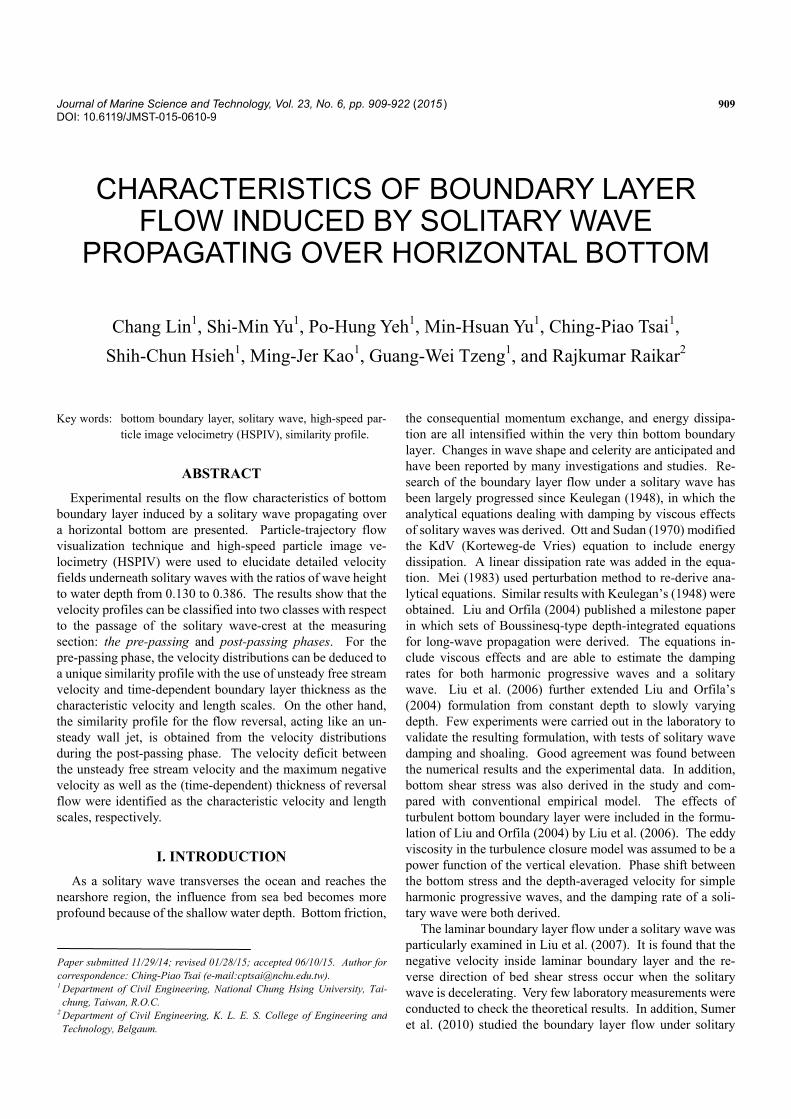
Key words: bottom boundary layer, solitary wave, high-speed par-ticle image velocimetry (HSPIV), similarity profile.

ABSTRACT

Experimental results on the flow characteristics of bottom boundary layer induced by a solitary wave propagating over a horizontal bottom are presented. Particle-trajectory flow visualization technique and high-speed particle image ve-locimetry (HSPIV) were used to elucidate detailed velocity fields underneath solitary waves with the ratios of wave height to water depth from 0.130 to 0.386. The results show that the velocity profiles can be classified into two classes with respect to the passage of the solitary wave-crest at the measuring section: the pre-passing and post-passing phases. For the pre-passing phase, the velocity distributions can be deduced to a unique similarity profile with the use of unsteady free stream velocity and time-dependent boundary layer thickness as the characteristic velocity and length scales. On the other hand, the similarity profile for the flow reversal, acting like an un-steady wall jet, is obtained from the velocity distributions during the post-passing phase. The velocity deficit between the unsteady free stream velocity and the maximum negative velocity as well as the (time-dependent) thickness of reversal flow were identified as the characteristic velocity and length scales, respectively.

I. INTRODUCTION

As a solitary wave transverses the ocean and reaches the nearshore region, the influence from sea bed becomes more profound because of the shallow water depth. Bottom friction,

the consequential momentum exchange, and energy dissipa-tion are all intensified within the very thin bottom boundary layer. Changes in wave shape and celerity are anticipated and have been reported by many investigations and studies. Re-search of the boundary layer flow under a solitary wave has been largely progressed since Keulegan (1948), in which the analytical equations dealing with damping by viscous effects of solitary waves was derived. Ott and Sudan (1970) modified the KdV (Korteweg-de Vries) equation to include energy dissipation. A linear dissipation rate was added in the equa-tion. Mei (1983) used perturbation method to re-derive ana-lytical equations. Similar results with Keulegan’s (1948) were obtained. Liu and Orfila (2004) published a milestone paper in which sets of Boussinesq-type depth-integrated equations for long-wave propagation were derived. The equations in-clude viscous effects and are able to estimate the damping rates for both harmonic progressive waves and a solitary wave. Liu et al. (2006) further extended Liu and Orfila’s (2004) formulation from constant depth to slowly varying depth. Few experiments were carried out in the laboratory to validate the resulting formulation, with tests of solitary wave damping and shoaling. Good agreement was found between the numerical results and the experimental data. In addition, bottom shear stress was also derived in the study and com-pared with conventional empirical model. The effects of turbulent bottom boundary layer were included in the formu-lation of Liu and Orfila (2004) by Liu et al. (2006). The eddy viscosity in the turbulence closure model was assumed to be a power function of the vertical elevation. Phase shift between the bottom stress and the depth-averaged velocity for simple harmonic progressive waves, and the damping rate of a soli-tary wave were both derived.

The laminar boundary layer flow under a solitary wave was particularly examined in Liu et al. (2007). It is found that the negative velocity inside laminar boundary layer and the re-verse direction of bed shear stress occur when the solitary wave is decelerating. Very few laboratory measurements were conducted to check the theoretical results. In addition, Sumer et al. (2010) studied the boundary layer flow under solitary

Paper submitted 11/29/14; revised 01/28/15; accepted 06/10/15. Author for correspondence: Ching-Piao Tsai (e-mail:cptsai@nchu.edu.tw). 1 Department of Civil Engineering, National Chung Hsing University, Tai-chung, Taiwan, R.O.C.

2 Department of Civil Engineering, K. L. E. S. College of Engineering and Technology, Belgaum.

910 Journal of Marine Science and Technology, Vol. 23, No. 6 (2015 )

wavemaker

solitary wave

8 m

14 m

Ar+ Laser

wave dissipator

12 cmFOV B

FOV A

O

Y

X1 cm

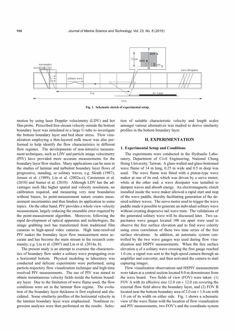
Fig. 1. Schematic sketch of experimental setup.

motion by using laser Doppler velocimetry (LDV) and hot film probe. Prescribed free-stream velocity outside the bottom boundary layer was simulated in a large U-tube to investigate the bottom boundary layer and bed shear stress. Flow visu-alization employing a thin-layered milk tracer was also per-formed to help identify the flow characteristics in different flow regimes. The developments of non-intrusive measure-ment techniques, such as LDV and particle image velocimetry (PIV) have provided more accurate measurements for the boundary layer flow studies. Many applications can be seen in the studies of laminar and turbulent boundary layer flows of progressive, standing, or solitary waves, e.g. Sleath (1987); Jensen et al. (1989); Lin et al. (2002a-c); Carstensen et al. (2010) and Sumer et al. (2010). Although LDV has the ad-vantages such like higher spatial and velocity resolution, no calibration required, and measuring very near boundaries without biases, its point-measurement nature creates meas-urement uncertainties and thus hinders its application to some topics. On the other hand, PIV provides a whole view velocity measurement, largely reducing the ensemble error required by the point-measurement algorithm. Moreover, following the rapid development of optical apparatus and technologies, the image grabbing tool has transformed from traditional film cameras to high-speed video cameras. High time-resolved PIV makes the boundary layer flow measurement more ac-curate and has become the main stream in the research com-munity, e.g. Liu et al. (2007) and Lin et al. (2014a, b).

The present study is an attempt to examine the characteris-tics of boundary flow under a solitary wave propagating over a horizontal bottom. Physical modeling in laboratory was conducted and delicate experiments were performed, using particle-trajectory flow visualization technique and high-time resolved PIV measurements. The use of PIV was aimed to obtain instantaneous velocity fields inside the bottom bound-ary layer. Due to the limitation of wave flume used, the flow conditions were set in the laminar flow regime. The evolu- tion of the boundary layer thickness is first explored and elu-cidated. Some similarity profiles of the horizontal velocity in the laminar boundary layer were emphasized. Nonlinear re-gression analyses were then performed on the results. Selec-

tion of suitable characteristic velocity and length scales amongst various alternatives was studied to derive similarity profiles in the bottom boundary layer.

II. EXPERIMENTATION

1. Experimental Setup and Conditions

The experiments were conducted in the Hydraulic Labo-ratory, Department of Civil Engineering, National Chung Hsing University, Taiwan. A glass-walled and glass-bottomed wave flume of 14 m long, 0.25 m wide and 0.5 m deep was used. The wave flume was fitted with a piston-type wave maker at one of its end, which was driven by a servo motor; while at the other end, a wave dissipater was installed to dampen waves and absorb energy. An electromagnetic clutch installed inside the wave maker allowed a rapid start and stop of the wave paddle, thereby facilitating generation of the de-sired solitary waves. The servo motor used to trigger the wave paddle made it possible to generate an individual solitary wave without creating dispersive tail wave train. The validations of the generated solitary wave will be discussed later. Two ca-pacitance wave gauges located 100 cm apart were used to observe the free surface elevation and to find wave celerity using cross correlation of these two time series of the free surface elevations. In addition, an automatic system con-trolled by the two wave gauges was used during flow visu-alization and HSPIV measurements. When the free surface elevation η of a solitary wave crossing the first gauge reached 1.0 cm, a signal was sent to the high-speed camera through an amplifier and converter, and then activated the camera to start capturing images.

Flow visualization observations and HSPIV measurements were taken at a central section located 8.0 m downstream from the wave board. Two fields of view (FOV) were taken: (1) FOV A with its effective size 12.0 cm 12.0 cm covering the external flow field above the boundary layer, and (2) FOV B located near the bottom boundary area of 2.0 cm 1.0 cm with 1.0 cm of its width on either side. Fig. 1 shows a schematic view of the wave flume with the location of flow visualization and PIV measurements, two FOV’s and the coordinate system

C. Lin et al.: Characteristics of Boundary Layer Flow Induced by Solitary Wave Propagating over Horizontal Bottom 911

Table 1. Details of experimental conditions.

Case Wave height

H (cm) Water depth

h (cm)

H

h Wave celerity

c (cm/s) Reynolds number

R1 Reynolds number

R2

A 1.3 10 0.130 104.9 1.1 104 4.6 103

B 1.2 7 0.171 90.1 8.9 103 4.2 103

C 1.5 7 0.214 90.9 1.1 104 5.6 103

D 2.1 8 0.263 98.0 1.6 104 8.9 103

E 1.9 7 0.271 93.5 1.4 104 8.0 103

F 2.9 8 0.363 102.0 1.9 104 1.1 104

G 2.7 7 0.386 99.0 1.8 104 1.1 104

used in the study. The origin of the coordinate system is lo-cated at the bottom center of FOV B with X along the bottom of the flume in the wave-motion direction, and Y normal to the bottom of the flume. The time t = 0 indicates the moment when the crest of the solitary wave crosses the position X = 0. Seven test cases were carried out with the ratio of wave height to water depth, H/h, ranging from 0.130 to 0.386.

Table 1 lists the wave condition and flow property of each tested case. The wave celerity in the table was measured value and to be compared with theoretical formula (discussed in the latter section). Two different Reynolds numbers are defined and listed in the table. The first Reynolds number is defined as R1 = hU/ν, where h represents the still water depth, U is the maximum free stream velocity at the edge of bottom boundary layer [= (u)max] and ν denotes the kinematic viscosity of water. Herein, the length scale a of the second Reynolds number R2 (= aU/ν) is half of the stroke of the water particle displacement in the free stream (Carstensen et al., 2010 and Sumer et al., 2010). The ranges of R1 and R2 in this study vary from 8.9 103 to 1.9 104 and from 4.2 103 to 1.1 104, respectively. As pointed out by Sumer et al. (2010), the boundary layer flow experiences three kinds of flow regimes as R2 increases: (1) laminar if R2 < 2 105; (2) laminar with vortex tube if 2 105 < R2 < 5 105; and (3) transitional if R2 > 5 105. Based on the R2 values in the classification of Sumer et al. (2010), flow regime in the present experiments is of the laminar boundary layer.

2. Particle-Trajectory Flow Visualization Technique

The flow structure within the wave field was visualized using particle trajectory flow visualization technique. Water in the wave flume was mixed with Titanium Dioxide particles of mean diameter 1.8 μm for illumination under laser light sheet. The settling velocity (i.e., fall velocity) of a spherical titanium dioxide particles determined by Stoke’s law is 4.5 10-4 cm/s, which is much smaller than the wave celerity c and the representative particle velocity in the present study. A 5 W argon-ion laser (Coherent Innova-90) was employed as a light source; laser beam was reflected by a glass cylinder of 0.57 cm diameter and spread into a fan-shaped light sheet of 1.5 mm thick, see Fig. 1.

The light sheet was directed upward into the flow region

through the glass bottom along the flume center line to illu-minate the 2-D motion of the tracing particles. An image recording system, which is a 10-bit complementary metal-oxide semiconductor (CMOS) high-speed digital camera (Phantom V5.1) with resolution of 1024 1024 pixels and maximum framing rate of 1200 Hz, was used to capture particle-laden images of the wave field. For FOV B, which is close to the bottom boundary area, the digital camera had 1024 1024 pixel resolution, 40 Hz framing rate, and focal length 200 mm; while in the external flow field (FOV A) the camera settings were 1024 512 pixel resolution, 20 Hz framing rate, and 60 mm focal length.

3. Velocity Measurements by HSPIV

A HSPIV system was employed to measure the two- dimensional velocity field in and near the bottom boundary layer induced by a solitary wave as it propagates over the horizontal bottom. The HSPIV system consists of an ar-gon-ion laser as light source and a high speed camera to cap-ture the images. The laser, optics for laser-light sheeting, seeding particles, and high speed camera used for the HSPIV measurements are all the same as those used in the flow visu-alization tests. A Nikon 200 mm lens was mounted on the camera to allow high resolution image-capturing and adequate magnification. Before performing the cross-correlation cal-culation for the velocity field, the following two procedures were used for the images captured by HSPIV. Firstly, all the images were processed via the Laplacian edge-enhancement technique (Adrain and Westerweel, 2011) to intensify the brightness of the particles. Secondly, following the image- processing steps described in the hybrid digital particle- tracking velocimetry technique (Cowen and Monismith, 1997), after contrast enhancement, the images were deducted from the background images to remove any constant noise source. Velocity fields in and near the boundary layer were then de-termined by cross-correlation analysis. The interrogation windows of 32 32 pixels with 50% overlap were used in the analysis. Note that 15 runs of test were completed repeatedly for each experimental case. Ensemble average was then used to average the data at the same time instant in each realization. The resulting averaged horizontal velocity is hereafter termed as horizontal velocity u.

912 Journal of Marine Science and Technology, Vol. 23, No. 6 (2015 )

(b)

0 0.1 0.2 0.3 0.4 0.51

1.1

1.2

1.3Present StudyYu (2011)Lin et al. (2005)Daily and Stephan (1953)Theory

c/ g

h

H/h

01086420-2-6-8-10 -4

0.25

0.5

T(a)

H/h = 0.263MeasurementsTheoretical profile

/H

η

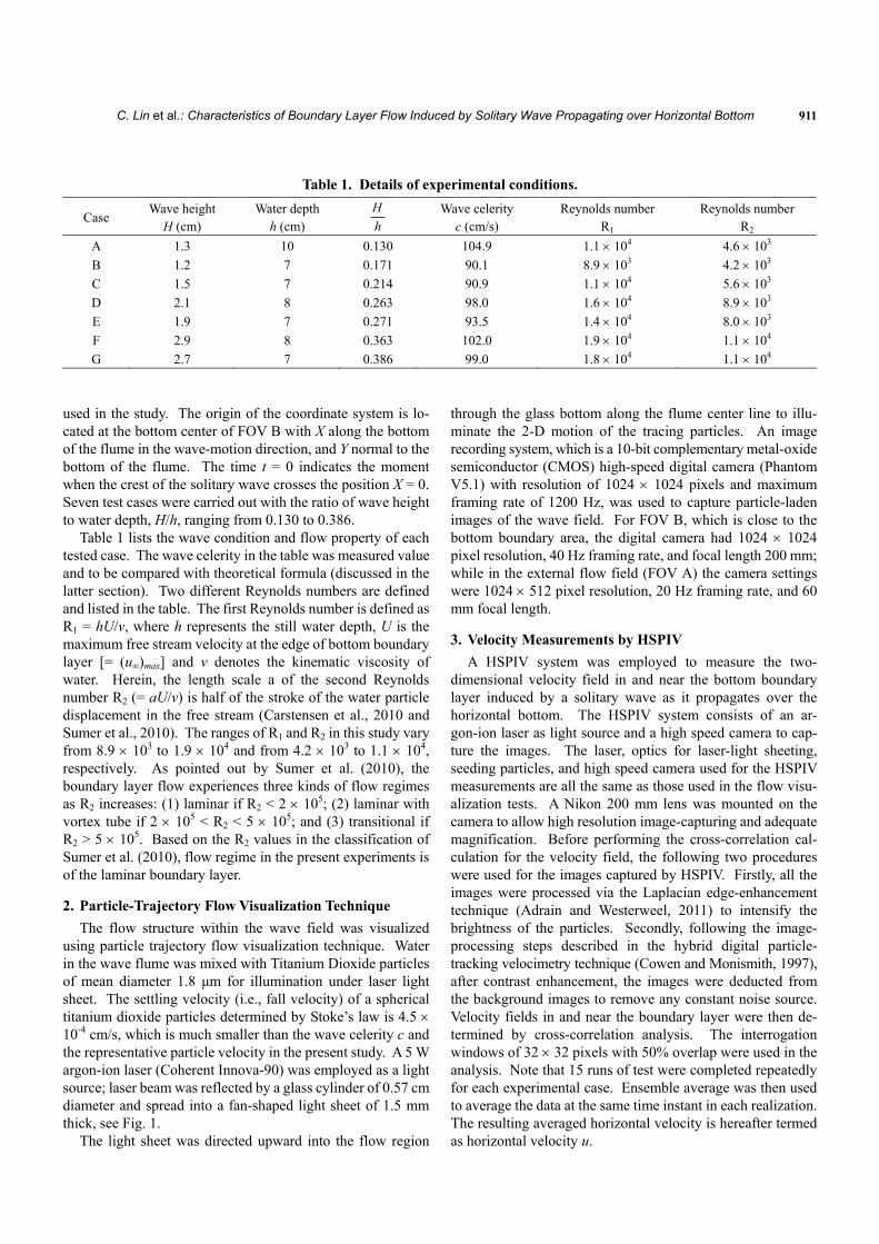
Fig. 2. (a) Free surface profile of Case D, and (b) validation of solitary

wave celerity.

III. VERIFICATIONS OF WAVE PROFILE AND VELOCITY

1. Validation of Solitary Wave Generation

The wave maker was fitted with high precision servo motor system, which could generate a solitary wave nearly without dispersive tail wave train. The generated solitary waves were generated by the procedure described in Goring (1978). Along with the generated solitary wave, its wave celerity was also assessed. Fig. 2(a) presents the comparison of non-dimensional time history of the free surface elevation between the gener-ated solitary wave and the theoretical wave profile given by

23

3( , ) sech ( )

4

HX t H X ct

h

(1)

where the wave celerity c can be obtained as [g(H + h)]1/2. It is interesting to observe a good conformity between these two. Besides, the comparison of wave celerity is also illustrated in Fig. 2(b). Satisfactory agreements can be clearly seen be-tween the generated waves in the present study and the data of Daily and Stephan (1953) and Lin et al. (2005, 2006).

2. Verification of Velocity Measured by HSPIV

Parallel to the HSPIV system, a fiber LDV was also used to verify the velocity measurements made by HSPIV. The LDV equipment was a two-component color burst-based, four-beam fiber-optic system (TSI System 90-3) with a 5 W argon-ion laser tube (Coherent Innova 90). Detailed descriptions of the LDV system can be referred to Lin et al. (2003, 2009). Herein,

0.4

Y (c

m)

0.3

0.2

0.1

0

12840−4 12840−4 12840−4 12840−412840−4 12840−4u (cm/s) u (cm/s) u (cm/s) u (cm/s) u (cm/s)u (cm/s)

0.4

0.3

0.2

0.1

0

Y (c

m)

T = 0 T = 5 T = 4 T = 3 T = 2 T = 1

T = −5 T = 0 T = −1 T = −2 T = −3 T = −4

16

12840−4 12840−4 12840−4 12840−412840−4 12840−4u(cm/s) u (cm/s) u (cm/s) u (cm/s) u (cm/s)u (cm/s)

16

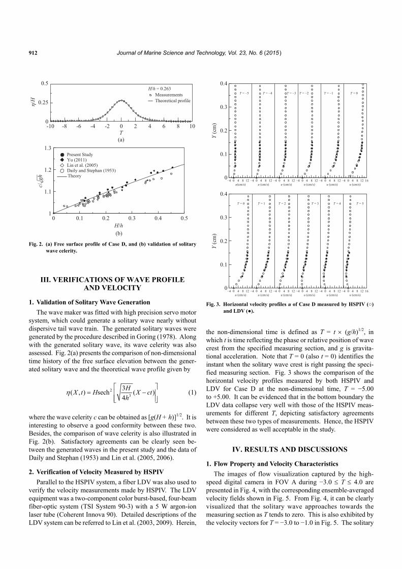
Fig. 3. Horizontal velocity profiles u of Case D measured by HSPIV (○)

and LDV (●).

the non-dimensional time is defined as T = t (g/h)1/2, in which t is time reflecting the phase or relative position of wave crest from the specified measuring section, and g is gravita-tional acceleration. Note that T = 0 (also t = 0) identifies the instant when the solitary wave crest is right passing the speci-fied measuring section. Fig. 3 shows the comparison of the horizontal velocity profiles measured by both HSPIV and LDV for Case D at the non-dimensional time, T = −5.00 to +5.00. It can be evidenced that in the bottom boundary the LDV data collapse very well with those of the HSPIV meas-urements for different T, depicting satisfactory agreements between these two types of measurements. Hence, the HSPIV were considered as well acceptable in the study.

IV. RESULTS AND DISCUSSIONS

1. Flow Property and Velocity Characteristics

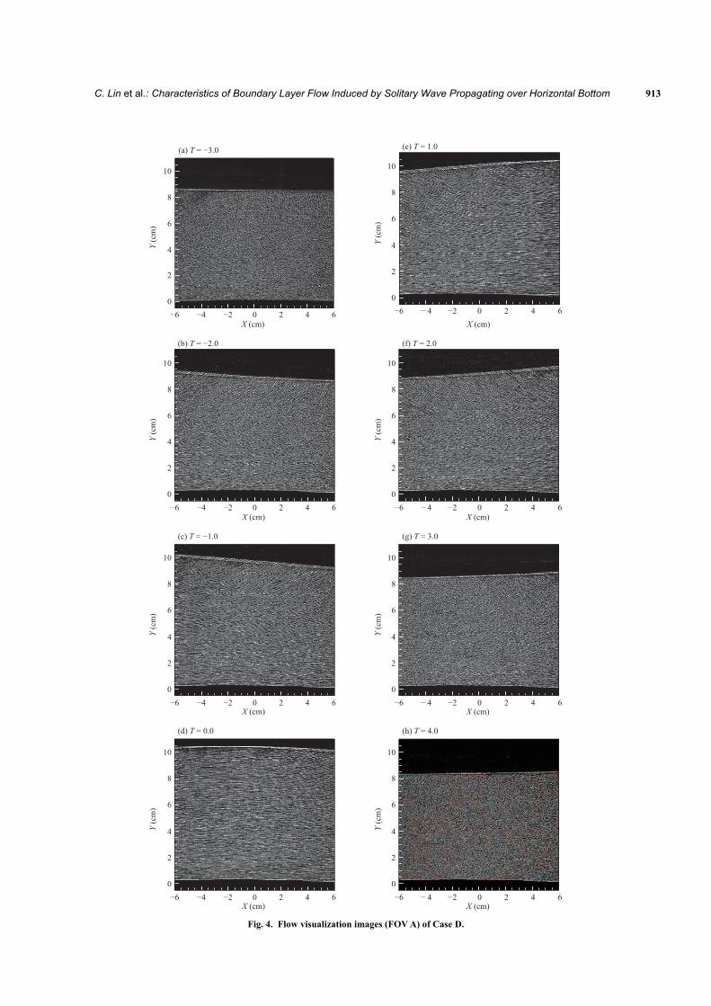
The images of flow visualization captured by the high- speed digital camera in FOV A during −3.0 T 4.0 are presented in Fig. 4, with the corresponding ensemble-averaged velocity fields shown in Fig. 5. From Fig. 4, it can be clearly visualized that the solitary wave approaches towards the measuring section as T tends to zero. This is also exhibited by the velocity vectors for T = −3.0 to −1.0 in Fig. 5. The solitary

C. Lin et al.: Characteristics of Boundary Layer Flow Induced by Solitary Wave Propagating over Horizontal Bottom 913

Y (c

m)

(f) T = 2.0

X (cm)

8

6

4

2

0

10

0−6 − 4 −2 2 4 6

Y (c

m)

(g) T = 3.0

X (cm)

8

6

4

2

0

10

0−6 − 4 −2 2 4 6

Y (c

m)

(h) T = 4.0

X (cm)

8

6

4

2

0

10

0−6 − 4 −2 2 4 6

Y (c

m)

(e) T = 1.0

8

6

4

2

0

X (cm)

10

0−6 − 4 −2 2 4 6

(c) T = −1.0

X (cm)

8

6

4

2

0

10

Y (c

m)

0−6 −4 −2 2 4 6

(d) T = 0.0

X (cm)

Y (c

m)

8

6

4

2

0

10

0−6 −4 −2 2 4 6

Y (c

m)

(a) T = −3.0

X (cm)

8

6

4

2

0

10

0−6 −4 −2 2 4 6

X (cm)

(b) T = −2.0

8

6

4

2

0

10

Y (c

m)

0−6 −4 −2 2 4 6

Fig. 4. Flow visualization images (FOV A) of Case D.

914 Journal of Marine Science and Technology, Vol. 23, No. 6 (2015 )

(a) T = −3.0

X (cm)

Y (c

m)

8

6

4

2

0

10

10 cm/s (e) T = 1.0

8

6

4

2

0

Y (c

m)

X (cm)

10

10 cm/s

0−6 −4 −2 2 4 6 0−6 −4 −2 2 4 6

54

12

109876

321

11

cm/s

54

12

109876

321

11

cm/s

10 cm/s 10 cm/s (b) T = −2.0

X (cm)

Y (c

m)

8

6

4

2

0

10

(f) T = 2.0

X (cm)

Y (c

m)

8

6

4

2

0

10

0−6 −4 −2 2 4 6 0−6 −4 −2 2 4 6

54

12

109876

321

11

cm/s

54

12

109876

321

11

cm/s

10 cm/s 10 cm/s (c) T = −1.0

X (cm)

Y (c

m)

8

6

4

2

0

10

(g) T = 3.0

X (cm)

Y (c

m)

8

6

4

2

0

10

0−6 −4 −2 2 4 6 0−6 −4 −2 2 4 6

54

12

109876

321

11

cm/s

54

12

109876

321

11

cm/s

10 cm/s 10 cm/s (d) T = 0.0

X (cm)

Y (c

m)

8

6

4

2

0

10

0−6 −4 −2 2 4 6 0−6 −4 −2 2 4 6

(h) T = 4.0

X (cm)

Y (c

m)

8

6

4

2

0

10

54

12

109876

321

11

cm/s

54

12

109876

321

11

cm/s

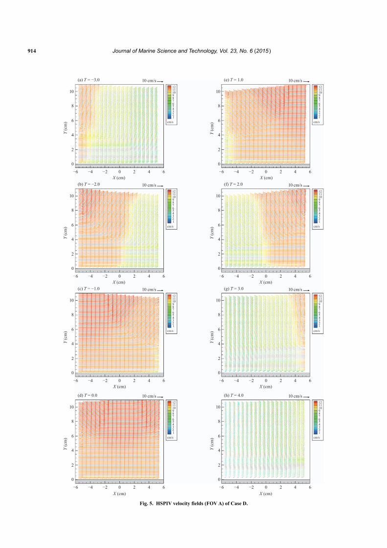
Fig. 5. HSPIV velocity fields (FOV A) of Case D.

C. Lin et al.: Characteristics of Boundary Layer Flow Induced by Solitary Wave Propagating over Horizontal Bottom 915

(e) T = 1.0

Y (c

m)

(a) T = −3.0

X (cm)

0.6

0.4

0.2

0

0.8

0−0.6−0.8 −0.4 −0.2 0.2 0.4 0.6X (cm)

0−0.6−0.8 −0.4 −0.2 0.2 0.4 0.6

(g) T = 3.0(c) T = −1.0

Y (c

m)

0.6

0.4

0.2

0

0.8

X (cm) 0−0.6−0.8 −0.4 −0.2 0.2 0.4 0.6

X (cm) 0−0.6−0.8 −0.4 −0.2 0.2 0.4 0.6

(h) T = 4.0(d) T = 0.0

Y (c

m)

0.6

0.4

0.2

0

0.8

X (cm) 0−0.6−0.8 −0.4 −0.2 0.2 0.4 0.6

X (cm) 0−0.6−0.8 −0.4 −0.2 0.2 0.4 0.6

(f) T = 2.0

Y (c

m)

0.6

0.4

0.2

0

0.8Y

(cm

)

0.6

0.4

0.2

0

0.8

Y (c

m)

0.6

0.4

0.2

0

0.8

Y (c

m)

0.6

0.4

0.2

0

0.8

Y (c

m)

0.6

0.4

0.2

0

0.8

X (cm) 0−0.6−0.8 −0.4 −0.2 0.2 0.4 0.6

X (cm) 0−0.6−0.8 −0.4 −0.2 0.2 0.4 0.6

(b) T = −2.0

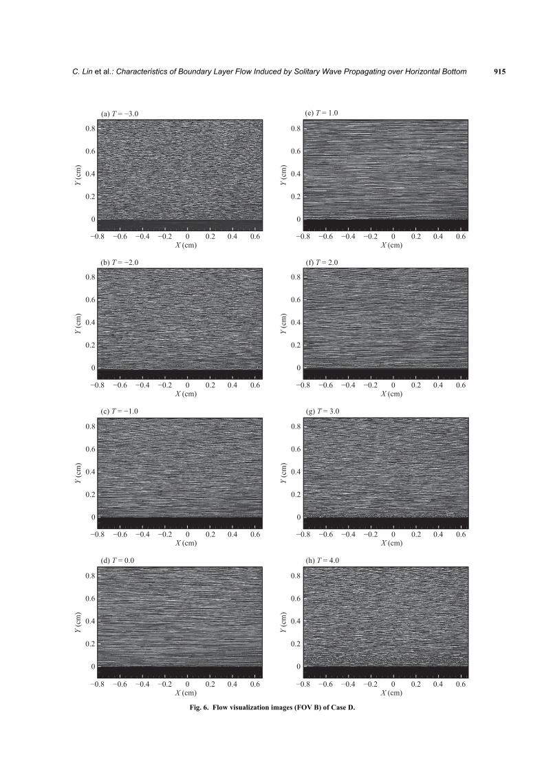
Fig. 6. Flow visualization images (FOV B) of Case D.

916 Journal of Marine Science and Technology, Vol. 23, No. 6 (2015 )

(a) T = −3.0 (e) T = 1.0

X (cm)

Y (c

m)

−0.8

0.8

0.6

0.4

0.2

0

Y (c

m)

0.8

0.6

0.4

0.2

0

−0.6 0.40.20−0.2−0.4 0.6X (cm)

−0.8 −0.6 0.40.20−0.2−0.4 0.6

10 cm/s 10 cm/s

54

12109876

321

11

cm/s

54

12109876

321

11

cm/s

(b) T = −2.0 (f) T = 2.0

Y (c

m)

0.8

0.6

0.4

0.2

0

Y (c

m)

0.8

0.6

0.4

0.2

0

X (cm) −0.8 −0.6 0.40.20−0.2−0.4 0.6

X (cm) −0.8 −0.6 0.40.20−0.2−0.4 0.6

10 cm/s 10 cm/s

54

12109876

321

11

cm/s

54

12109876

321

11

cm/s

(c) T = −1.0 (g) T = 3.0

Y (c

m)

0.8

0.6

0.4

0.2

0

Y (c

m)

0.8

0.6

0.4

0.2

0

X (cm) −0.8 −0.6 0.40.20−0.2−0.4 0.6

X (cm) −0.8 −0.6 0.40.20−0.2−0.4 0.6

10 cm/s 10 cm/s

54

12109876

321

11

cm/s

54

12109876

321

11

cm/s

(d) T = 0.0 (h) T = 4.0

Y (c

m)

0.8

0.6

0.4

0.2

0

Y (c

m)

0.8

0.6

0.4

0.2

0

X (cm) −0.8 −0.6 0.40.20−0.2−0.4 0.6

X (cm) −0.8 −0.6 0.40.20−0.2−0.4 0.6

10 cm/s 10 cm/s

54

12109876

321

11

cm/s

54

12109876

321

11

cm/s

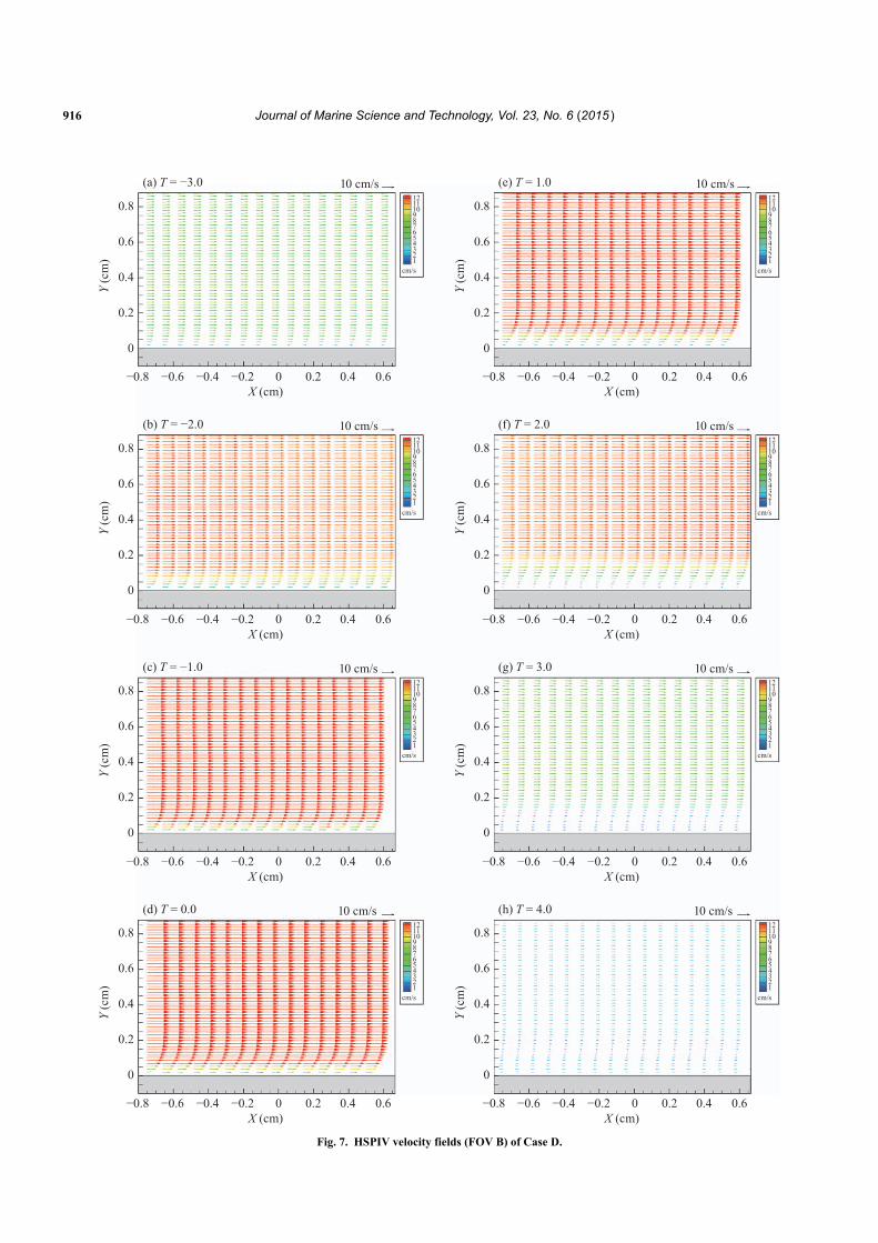
Fig. 7. HSPIV velocity fields (FOV B) of Case D.

C. Lin et al.: Characteristics of Boundary Layer Flow Induced by Solitary Wave Propagating over Horizontal Bottom 917

0.05(b)

5 4 3 2 1 0X/h

−1 −2 −3 −4 −5

−5 −4 −3 −2 −1 0T

1 2 3 4 5

0.04

Y/h

0.1

0.05

0

(a)

Y/h

0.03

0.02

0.01

0

T = 1.0 T = 2.0 T = 2.2T = 1.8 T = 1.6T = 1.4T = 1.2

12840−4u (cm/s) u (cm/s) u (cm/s) u (cm/s) u (cm/s) u (cm/s)u (cm/s)

1612840−4 1612840−4 1612840−4 1612840−4 1612840−4 1612840−4 16

5 cm/s

54

12

109876

321

11

cm/s

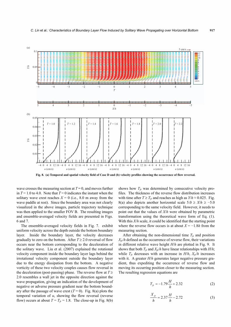
Fig. 8. (a) Temporal and spatial velocity field of Case D and (b) velocity profiles showing the occurrence of flow reversal.

wave crosses the measuring section at T = 0, and moves further in T = 1.0 to 4.0. Note that T = 0 indicates the instant when the solitary wave crest reaches X = 0 (i.e., 8.0 m away from the wave paddle at rest). Since the boundary area was not clearly visualized in the above images, particle trajectory technique was then applied to the smaller FOV B. The resulting images and ensemble-averaged velocity fields are presented in Figs. 6 and 7.

The ensemble-averaged velocity fields in Fig. 7. exhibit uniform velocity across the depth outside the bottom boundary layer. Inside the boundary layer, the velocity decreases gradually to zero on the bottom. After T 2.0 reversal of flow occurs near the bottom corresponding to the deceleration of the solitary wave. Liu et al. (2007) explained the rotational velocity component inside the boundary layer lags behind the irrotational velocity component outside the boundary layer due to the energy dissipation from the bottom. A negative vorticity of these two velocity couples causes flow reversal in the deceleration (post-passing) phase. The reverse flow at T 2.0 resembles a wall jet in the opposite direction against the wave propagation, giving an indication of the development of negative or adverse pressure gradient near the bottom bound-ary after the passage of wave crest (T = 0). Fig. 8(a) plots the temporal variation of u, showing the flow reversal (reverse flow) occurs at about T = Tfr = 1.8. The close-up in Fig. 8(b)

shows how Tfr was determined by consecutive velocity pro-files. The thickness of the reverse flow distribution increases with time after T Tfr and reaches as high as Y/h ≈ 0.025. Fig. 8(a) also depicts another horizontal scale 5.0 X/h −5.0 corresponding to the same velocity field. However, it needs to point out that the values of X/h were obtained by parametric transformation using the theoretical wave form of Eq. (1). With this X/h scale, it could be identified that the starting point where the reverse flow occurs is at about X = −1.8h from the measuring section.

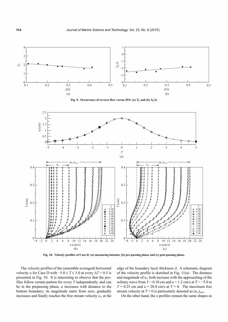
After obtaining the non-dimensional time Tfr and position Xfr/h defined as the occurrence of reverse flow, their variations in different relative wave height H/h are plotted in Fig. 9. It shows that both Tfr and Xfr/h have linear relationships with H/h; while Tfr decreases with an increase in H/h, Xfr/h increases with it. A greater H/h generates larger negative pressure gra-dient, thus expediting the occurrence of reverse flow and moving its occurring position closer to the measuring section. The resulting regression equations are

1.79 2.32fr

HT

h (2)

2.37 2.72frX H

h h (3)

918 Journal of Marine Science and Technology, Vol. 23, No. 6 (2015 )

(a)

00.1

1

2

4

3

0.2 0.3 0.4 0.5

T fr

H/h(b)

0.1 0.50.40.30.2

−3

−4

−2

−1

0

1

X fr/h

H/h

Fig. 9. Occurrence of reverse flow versus H/h: (a) Tfr and (b) Xfr/h.

−5 −4 −3 −2 −1 543210

2

0

0.5

1

1.5

2.5

T(a)

(cm

)η

Y (c

m)

Y (c

m)

0.4

0.1

0.2

0.3

0

(b)

u∞(u∞)max

−4 16 188−2 0 2 4 6 10 12 14 20 22 24u (cm/s)

0.00−0.50−1.00−1.50−2.00−2.50−3.00−3.50−4.00−4.50−5.00

0.4

0.1

0.2

0.3

0

(c)

u∞

−4 16 188−2 0 2 4 6 10 12 14 20 22 24u (cm/s)

5.004.504.003.503.002.502.001.501.000.500.00

TT

(u∞)max

Fig. 10. Velocity profiles of Case D: (a) measuring instants, (b) pre-passing phase and (c) post-passing phase.

The velocity profiles of the (ensemble-averaged) horizontal

velocity u for Case D with −5.0 T 5.0 at every T = 0.5 is presented in Fig. 10. It is interesting to observe that the pro-files follow certain pattern for every T independently, and can be in the prepassing phase, u increases with distance to the bottom boundary; its magnitude starts from zero, gradually increases and finally reaches the free stream velocity u at the

edge of the boundary layer thickness . A schematic diagram of the velocity profile is sketched in Fig. 11(a). The distance and magnitude of u both increase with the approaching of the solitary wave from Y = 0.10 cm and u = 1.2 cm/s at T = −5.0 to Y = 0.25 cm and u = 20.0 cm/s at T = 0. The maximum free stream velocity at T = 0 is particularly denoted as (u)max.

On the other hand, the u profiles remain the same shapes as

C. Lin et al.: Characteristics of Boundary Layer Flow Induced by Solitary Wave Propagating over Horizontal Bottom 919

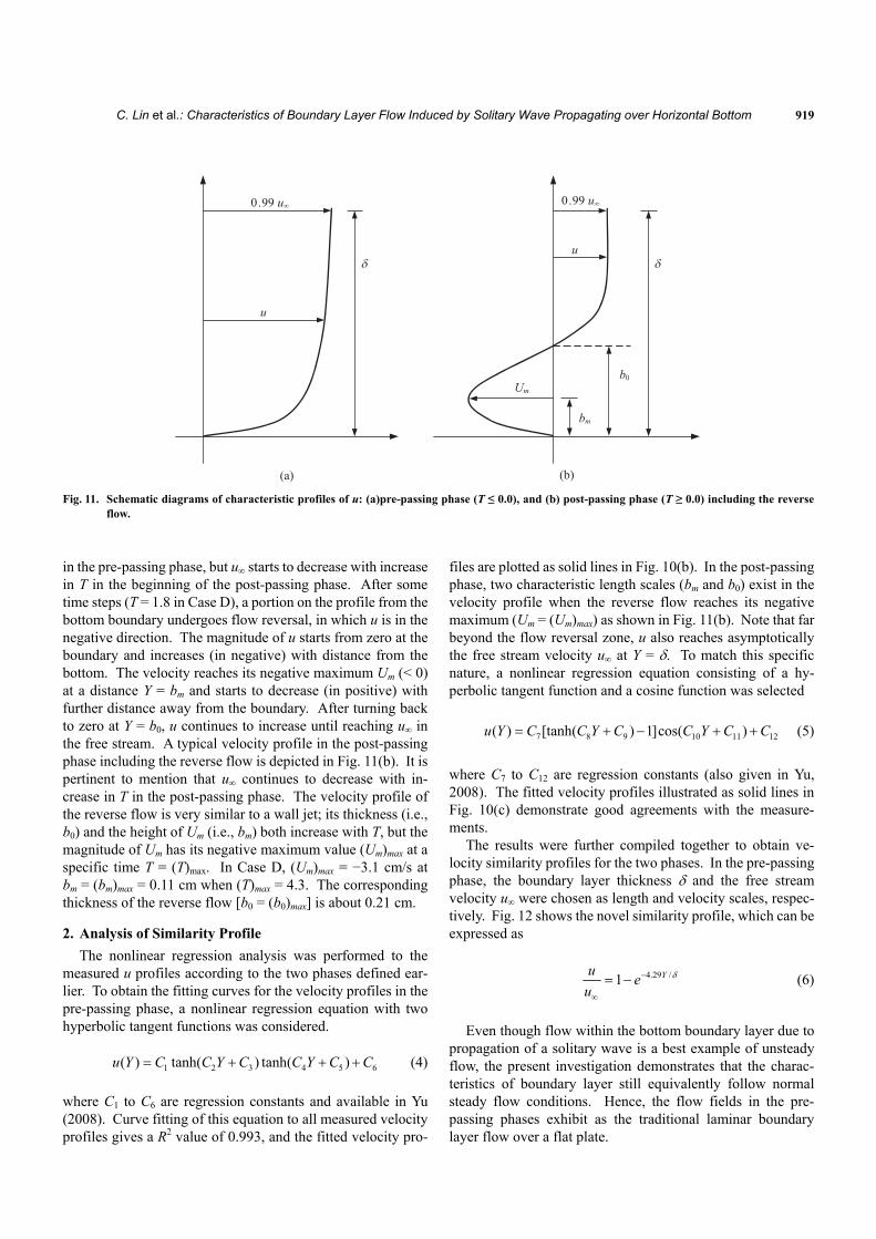
(a)

0.99 u∞

u

δ

0.99 u∞

uδ

b0

bm

Um

(b) Fig. 11. Schematic diagrams of characteristic profiles of u: (a)pre-passing phase (T ≤ 0.0), and (b) post-passing phase (T ≥ 0.0) including the reverse

flow.

in the pre-passing phase, but u starts to decrease with increase in T in the beginning of the post-passing phase. After some time steps (T = 1.8 in Case D), a portion on the profile from the bottom boundary undergoes flow reversal, in which u is in the negative direction. The magnitude of u starts from zero at the boundary and increases (in negative) with distance from the bottom. The velocity reaches its negative maximum Um (< 0) at a distance Y = bm and starts to decrease (in positive) with further distance away from the boundary. After turning back to zero at Y = b0, u continues to increase until reaching u in the free stream. A typical velocity profile in the post-passing phase including the reverse flow is depicted in Fig. 11(b). It is pertinent to mention that u continues to decrease with in-crease in T in the post-passing phase. The velocity profile of the reverse flow is very similar to a wall jet; its thickness (i.e., b0) and the height of Um (i.e., bm) both increase with T, but the magnitude of Um has its negative maximum value (Um)max at a specific time T = (T)max. In Case D, (Um)max = −3.1 cm/s at bm = (bm)max = 0.11 cm when (T)max = 4.3. The corresponding thickness of the reverse flow [b0 = (b0)max] is about 0.21 cm.

2. Analysis of Similarity Profile

The nonlinear regression analysis was performed to the measured u profiles according to the two phases defined ear-lier. To obtain the fitting curves for the velocity profiles in the pre-passing phase, a nonlinear regression equation with two hyperbolic tangent functions was considered.

1 2 3 4 5 6( ) tanh( ) tanh( )u Y C C Y C C Y C C (4)

where C1 to C6 are regression constants and available in Yu (2008). Curve fitting of this equation to all measured velocity profiles gives a R2 value of 0.993, and the fitted velocity pro-

files are plotted as solid lines in Fig. 10(b). In the post-passing phase, two characteristic length scales (bm and b0) exist in the velocity profile when the reverse flow reaches its negative maximum (Um = (Um)max) as shown in Fig. 11(b). Note that far beyond the flow reversal zone, u also reaches asymptotically the free stream velocity u at Y = . To match this specific nature, a nonlinear regression equation consisting of a hy-perbolic tangent function and a cosine function was selected

7 8 9 10 11 12( ) [tanh( ) 1]cos( )u Y C C Y C C Y C C (5)

where C7 to C12 are regression constants (also given in Yu, 2008). The fitted velocity profiles illustrated as solid lines in Fig. 10(c) demonstrate good agreements with the measure-ments.

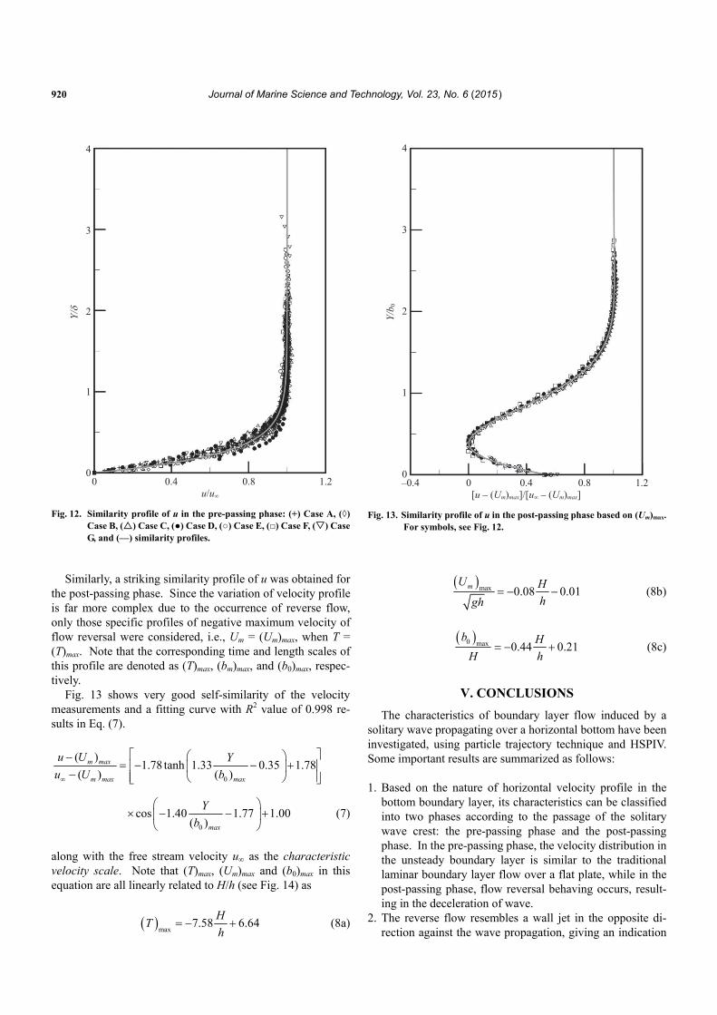
The results were further compiled together to obtain ve-locity similarity profiles for the two phases. In the pre-passing phase, the boundary layer thickness and the free stream velocity u were chosen as length and velocity scales, respec-tively. Fig. 12 shows the novel similarity profile, which can be expressed as

4.29 /1 Yue

u

(6)

Even though flow within the bottom boundary layer due to propagation of a solitary wave is a best example of unsteady flow, the present investigation demonstrates that the charac-teristics of boundary layer still equivalently follow normal steady flow conditions. Hence, the flow fields in the pre- passing phases exhibit as the traditional laminar boundary layer flow over a flat plate.

920 Journal of Marine Science and Technology, Vol. 23, No. 6 (2015 )

00

1

2

3

4

0.4u/u∞

0.8 1.2

Y/δ

Fig. 12. Similarity profile of u in the pre-passing phase: (+) Case A, (◊)

Case B, () Case C, (●) Case D, (○) Case E, (□) Case F, () Case G, and (—) similarity profiles.

Similarly, a striking similarity profile of u was obtained for

the post-passing phase. Since the variation of velocity profile is far more complex due to the occurrence of reverse flow, only those specific profiles of negative maximum velocity of flow reversal were considered, i.e., Um = (Um)max, when T = (T)max. Note that the corresponding time and length scales of this profile are denoted as (T)max, (bm)max, and (b0)max, respec-tively.

Fig. 13 shows very good self-similarity of the velocity measurements and a fitting curve with R2 value of 0.998 re-sults in Eq. (7).

0

( )1.78 tanh 1.33 0.35 1.78

( ) ( )m max

m max max

u U Y

u U b

0

cos 1.40 1.77 1.00( )max

Y

b

(7)

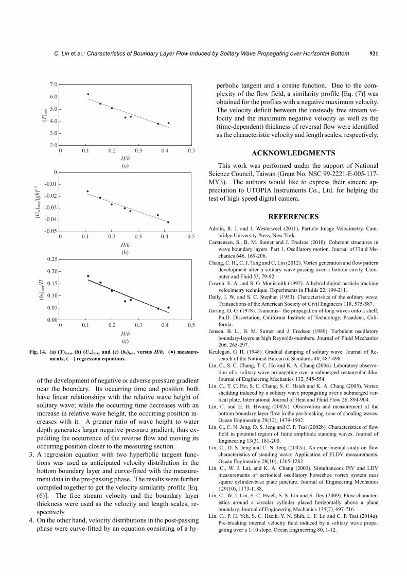
along with the free stream velocity u as the characteristic velocity scale. Note that (T)max, (Um)max and (b0)max in this equation are all linearly related to H/h (see Fig. 14) as

max7.58 6.64

HT

h

(8a)

–0.4 00

1

2

3

4

0.4[u – (Um)max]/[u∞ – (Um)max]

0.8 1.2

Y/b 0

Fig. 13. Similarity profile of u in the post-passing phase based on (Um)max.

For symbols, see Fig. 12.

max 0.08 0.01mU H

hgh

(8b)

0 max 0.44 0.21b H

H h

(8c)

V. CONCLUSIONS

The characteristics of boundary layer flow induced by a solitary wave propagating over a horizontal bottom have been investigated, using particle trajectory technique and HSPIV. Some important results are summarized as follows:

1. Based on the nature of horizontal velocity profile in the

bottom boundary layer, its characteristics can be classified into two phases according to the passage of the solitary wave crest: the pre-passing phase and the post-passing phase. In the pre-passing phase, the velocity distribution in the unsteady boundary layer is similar to the traditional laminar boundary layer flow over a flat plate, while in the post-passing phase, flow reversal behaving occurs, result-ing in the deceleration of wave.

2. The reverse flow resembles a wall jet in the opposite di-rection against the wave propagation, giving an indication

C. Lin et al.: Characteristics of Boundary Layer Flow Induced by Solitary Wave Propagating over Horizontal Bottom 921

2.0

3.0

4.0

5.0

6.0

7.0

0 0.1 0.2 0.3 0.4 0.5

-0.05

-0.04

-0.03

-0.02

-0.01

0

0 0.1 0.2 0.3 0.4 0.5H/h

0.00

0.05

0.10

0.15

0.20

0.25

0 0.1 0.2 0.3 0.4 0.5H/h

(b0) m

ax/H

(T) m

ax

(Um) m

ax/(g

h)0.

5

H/h

(b)

(c)

(a)

Fig. 14. (a) (T)max, (b) (Um)max and (c) (b0)max versus H/h. (●) measure-

ments, (—) regression equations. of the development of negative or adverse pressure gradient

near the boundary. Its occurring time and position both have linear relationships with the relative wave height of solitary wave; while the occurring time decreases with an increase in relative wave height, the occurring position in-creases with it. A greater ratio of wave height to water depth generates larger negative pressure gradient, thus ex-pediting the occurrence of the reverse flow and moving its occurring position closer to the measuring section.

3. A regression equation with two hyperbolic tangent func-tions was used as anticipated velocity distribution in the bottom boundary layer and curve-fitted with the measure-ment data in the pre-passing phase. The results were further compiled together to get the velocity similarity profile [Eq. (6)]. The free stream velocity and the boundary layer thickness were used as the velocity and length scales, re-spectively.

4. On the other hand, velocity distributions in the post-passing phase were curve-fitted by an equation consisting of a hy-

perbolic tangent and a cosine function. Due to the com-plexity of the flow field, a similarity profile [Eq. (7)] was obtained for the profiles with a negative maximum velocity. The velocity deficit between the unsteady free stream ve-locity and the maximum negative velocity as well as the (time-dependent) thickness of reversal flow were identified as the characteristic velocity and length scales, respectively.

ACKNOWLEDGMENTS

This work was performed under the support of National Science Council, Taiwan (Grant No. NSC 99-2221-E-005-117- MY3). The authors would like to express their sincere ap-preciation to UTOPIA Instruments Co., Ltd. for helping the test of high-speed digital camera.

REFERENCES

Adrain, R. J. and J. Westerweel (2011). Particle Image Velocimetry. Cam-bridge University Press, New York.

Carstensen, S., B. M. Sumer and J. Fredsøe (2010). Coherent structures in wave boundary layers. Part 1. Oscillatory motion. Journal of Fluid Me-chanics 646, 169-206.

Chang, C. H., C. J. Tang and C. Lin (2012). Vortex generation and flow pattern development after a solitary wave passing over a bottom cavity. Com-puter and Fluid 53, 79-92.

Cowen, E. A. and S. G. Monismith (1997). A hybrid digital particle tracking velocimetry technique. Experiments in Fluids 22, 199-211.

Daily, J. W. and S. C. Stephan (1953). Characteristics of the solitary wave. Transactions of the American Society of Civil Engineers 118, 575-58.

Goring, D. G. (1978). Tsunamis the propagation of long waves onto a shelf, Ph.D. Dissertation, California Institute of Technology, Pasadena, Cali-fornia.

Jensen, B. L., B. M. Sumer and J. Fredsoe (1989). Turbulent oscillatory boundary-layers at high Reynolds-numbers. Journal of Fluid Mechanics 206, 265-297.

Keulegan, G. H. (1948). Gradual damping of solitary wave. Journal of Re-search of the National Bureau of Standards 40, 48-498.

Lin, C., S. C. Chang, T. C. Ho and K. A. Chang (2006). Laboratory observa-tion of a solitary wave propagating over a submerged rectangular dike. Journal of Engineering Mechanics 132, 545-554.

Lin, C., T. C. Ho, S. C. Chang, S. C. Hsieh and K. A. Chang (2005). Vortex shedding induced by a solitary wave propagating over a submerged ver-tical plate. International Journal of Heat and Fluid Flow 26, 894-904.

Lin, C. and H. H. Hwung (2002a). Observation and measurement of the bottom boundary layer flow in the pre-breaking zone of shoaling waves. Ocean Engineering 29(12), 1479-1502.

Lin, C., C. N. Jeng, D. S. Jeng and C. P. Tsai (2002b). Characteristics of flow field in potential region of finite amplitude standing waves. Journal of Engineering 13(3), 181-200.

Lin, C., D. S. Jeng and C. N. Jeng (2002c). An experimental study on flow characteristics of standing wave: Application of FLDV measurements. Ocean Engineering 29(10), 1265-1282.

Lin, C., W. J. Lai, and K. A. Chang (2003). Simultaneous PIV and LDV measurements of periodical oscillatory horseshoe vortex system near square cylinder-base plate juncture. Journal of Engineering Mechanics 129(10), 1173-1188.

Lin, C., W. J. Lin, S. C. Hsieh, S. S. Lin and S. Dey (2009). Flow character-istics around a circular cylinder placed horizontally above a plane boundary. Journal of Engineering Mechanics 135(7), 697-716.

Lin, C., P. H. Yeh, S. C. Hseih, Y. N. Shih, L. F. Lo and C. P. Tsai (2014a). Pre-breaking internal velocity field induced by a solitary wave propa-gating over a 1:10 slope. Ocean Engineering 80, 1-12.

922 Journal of Marine Science and Technology, Vol. 23, No. 6 (2015 )

Lin, C., P. H. Yeh, M. J. Kao, M. H. Yu, S. C. Hseih, S. C. Chang, T. R. Wu and C. P. Tsai (2014b). Velocity fields inside near-bottom and boundary layer flow in pre-breaking zone of solitary wave propagating over a 1:10 slope. Journal of Waterways, Port, Coastal, and Ocean Engineering, ASCE.

Liu, P. L.-F. (2006). Turbulent boundary-layer effects on transient wave propagation in shallow water. Proceedings of the Royal Society A 462, 3481-3491.

Liu, P. L.-F. and A. Orfila (2004). Viscous effects on transient long-wave propagation. Journal of Fluid Mechanics 520, 83-92.

Liu, P. L.-F., G. Simarro, J. Vandever and A. Orfila (2006). Experimental and numerical investigation of viscous effects on solitary wave propagation in a wave tank. Coastal Engineering 53, 181-190.

Liu, P. L.-F., Y. S. Park and E. A. Cowen (2007). Boundary layer flow and bed shear stress under a solitary wave. Journal of Fluid Mechanics 54, 449-463.

Mei, C. C. (1983). The Applied Dynamics of Ocean Surface Waves, 2nd Ed., John Wiley and Sons.

Ott, E. and R. N. Sudan (1970). Damping of solitary waves. Physics of Fluids 13(6), 1432-1434.

Sleath, J. F. A. (1987). Turbulent oscillatory flow over rough beds. Journal of Fluid Mechanics 182, 369-409.

Sumer, B. M., P. M. Jensen, L. B. Sørensen, J. Fredsøe, P. L.-F. Liu and S. Carstensen (2010). Coherent structures in wave boundary layers-- Part 2. Solitary motion. Journal of Fluid Mechanics 646, 207-231.

Yu, S. M. (2008). The characteristics of bottom boundary layer flow induced by solitary wave. Master Thesis, National Chung Hsing University, Tai-wan. (in Chinese)

Yu, M. H. (2011). Study on the characteristics of bottom boundary layer flow induced by a solitary wave propagating over a sloping bottom. Master Thesis, National Chung Hsing University Taiwan. (in Chinese)