Characterisation of an electron source to ionize gasmolecules through electron ionization

Antonio BianchiUniversity of Torino, Italy

antonio.bianchi@studenti.unito.it

Supervisor: Andreas Przystawik

September 9, 2014DESY - Hamburg

Abstract

The electron ionization is a method to produce ions through the interactionbetween energetic electrons and gas molecules.The purposes of this project are to set up all necessary tools and to identify

the best operation parameters for the electron source in order to achieve optimalelectron ionization. A time-of-flight mass spectrometer is used to observe theionization of molecules hit with the electron beam.The characterisation of the electron source might be useful for testing the time-

of-flight spectrometer and all other devices, that are necessary for the next exper-iments in FLASH at DESY.

1

Contents

1 Introduction 3

2 Apparatus and experimental details 32.1 Vacuum chamber . . . . . . . . . . . . . . . . . . . . . . . . . . . . . . . 42.2 Electron source . . . . . . . . . . . . . . . . . . . . . . . . . . . . . . . . 52.3 Time-of-flight mass spectrometer . . . . . . . . . . . . . . . . . . . . . . 7

3 Data analysis 11

4 Results and discussion 18

5 Conclusions 20

6 Appendix 21

2

1 Introduction

Electron ionization (or electron impact ionization) is a useful method to produce ionsthrough the interaction between energetic electrons and gas molecules. The electronionization process is described by the following formula:

M + e− →Mn+ + n · e− with n = 1, 2, 3... (1)

where M is a gas molecule (in our case, argon gas) to analyze, e− is an electron whichinteracts with the gas molecule M and Mn+ is the resulting ion.

The purposes of the project, described in this report, are to set up all necessary toolsfor electron ionization and to identify the best operation parameters for the electronsource in order to achieve optimal electron ionization. The characterisation of the elec-tron source might be also useful for testing the time-of-flight spectrometer and all otherdevices for the next experiments at FLASH or other facilities.

2 Apparatus and experimental details

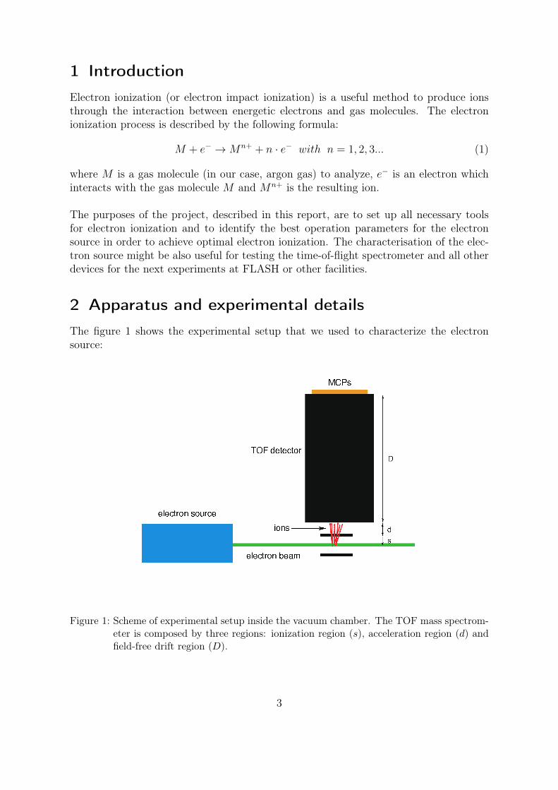
The figure 1 shows the experimental setup that we used to characterize the electronsource:

Figure 1: Scheme of experimental setup inside the vacuum chamber. The TOF mass spectrom-eter is composed by three regions: ionization region (s), acceleration region (d) andfield-free drift region (D).

3

An electron beam is used to ionize the gas molecules inside the vacuum chamber and thenthe ions are analyzed through a time-of-flight (TOF) mass spectrometer to determinatethe mass-to-charge ratio of each ion, formed by electron ionization.In the following paragraphs, we are going to discuss the vacuum chamber, the electronsource and the TOF mass spectrometer in detail.

2.1 Vacuum chamber

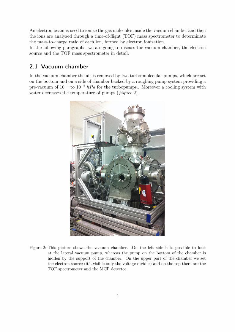
In the vacuum chamber the air is removed by two turbo-molecular pumps, which are seton the bottom and on a side of chamber backed by a roughing pump system providing apre-vacuum of 10−1 to 10−2 hPa for the turbopumps.. Moreover a cooling system withwater decreases the temperature of pumps (figure 2).

Figure 2: This picture shows the vacuum chamber. On the left side it is possible to lookat the lateral vacuum pump, whereas the pump on the bottom of the chamber ishidden by the support of the chamber. On the upper part of the chamber we setthe electron source (it’s visible only the voltage divider) and on the top there are theTOF spectrometer and the MCP detector.

4

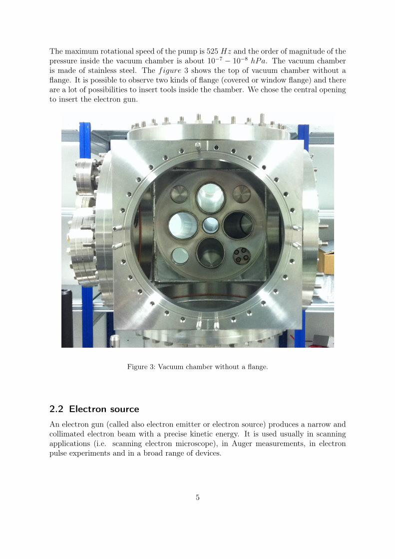
The maximum rotational speed of the pump is 525 Hz and the order of magnitude of thepressure inside the vacuum chamber is about 10−7 − 10−8 hPa. The vacuum chamberis made of stainless steel. The figure 3 shows the top of vacuum chamber without aflange. It is possible to observe two kinds of flange (covered or window flange) and thereare a lot of possibilities to insert tools inside the chamber. We chose the central openingto insert the electron gun.

Figure 3: Vacuum chamber without a flange.

2.2 Electron source

An electron gun (called also electron emitter or electron source) produces a narrow andcollimated electron beam with a precise kinetic energy. It is used usually in scanningapplications (i.e. scanning electron microscope), in Auger measurements, in electronpulse experiments and in a broad range of devices.

5

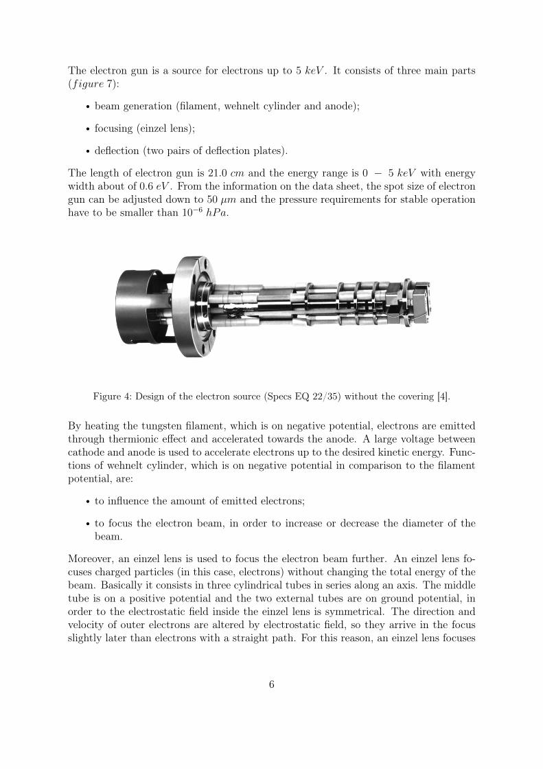
The electron gun is a source for electrons up to 5 keV . It consists of three main parts(figure 7):

beam generation (filament, wehnelt cylinder and anode);

focusing (einzel lens);

deflection (two pairs of deflection plates).

The length of electron gun is 21.0 cm and the energy range is 0 − 5 keV with energywidth about of 0.6 eV . From the information on the data sheet, the spot size of electrongun can be adjusted down to 50 µm and the pressure requirements for stable operationhave to be smaller than 10−6 hPa.

Figure 4: Design of the electron source (Specs EQ 22/35) without the covering [4].

By heating the tungsten filament, which is on negative potential, electrons are emittedthrough thermionic effect and accelerated towards the anode. A large voltage betweencathode and anode is used to accelerate electrons up to the desired kinetic energy. Func-tions of wehnelt cylinder, which is on negative potential in comparison to the filamentpotential, are:

to influence the amount of emitted electrons;

to focus the electron beam, in order to increase or decrease the diameter of thebeam.

Moreover, an einzel lens is used to focus the electron beam further. An einzel lens fo-cuses charged particles (in this case, electrons) without changing the total energy of thebeam. Basically it consists in three cylindrical tubes in series along an axis. The middletube is on a positive potential and the two external tubes are on ground potential, inorder to the electrostatic field inside the einzel lens is symmetrical. The direction andvelocity of outer electrons are altered by electrostatic field, so they arrive in the focusslightly later than electrons with a straight path. For this reason, an einzel lens focuses

6

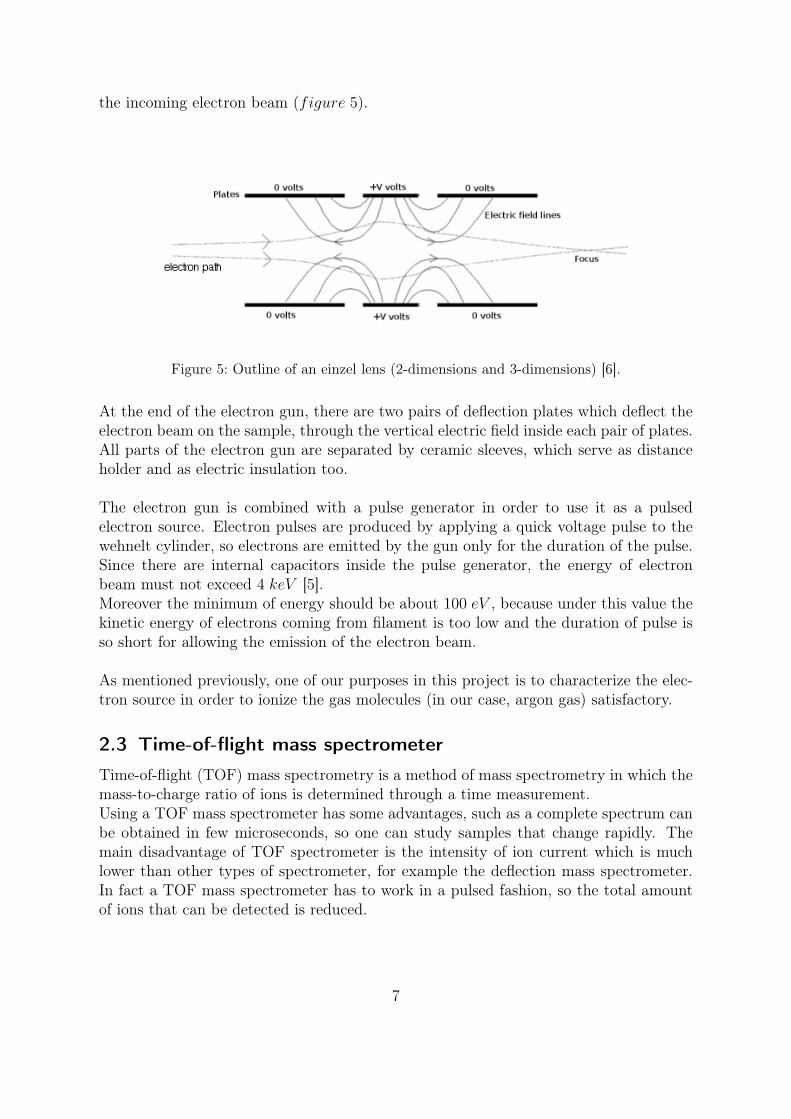
the incoming electron beam (figure 5).

Figure 5: Outline of an einzel lens (2-dimensions and 3-dimensions) [6].

At the end of the electron gun, there are two pairs of deflection plates which deflect theelectron beam on the sample, through the vertical electric field inside each pair of plates.All parts of the electron gun are separated by ceramic sleeves, which serve as distanceholder and as electric insulation too.

The electron gun is combined with a pulse generator in order to use it as a pulsedelectron source. Electron pulses are produced by applying a quick voltage pulse to thewehnelt cylinder, so electrons are emitted by the gun only for the duration of the pulse.Since there are internal capacitors inside the pulse generator, the energy of electronbeam must not exceed 4 keV [5].Moreover the minimum of energy should be about 100 eV , because under this value thekinetic energy of electrons coming from filament is too low and the duration of pulse isso short for allowing the emission of the electron beam.

As mentioned previously, one of our purposes in this project is to characterize the elec-tron source in order to ionize the gas molecules (in our case, argon gas) satisfactory.

2.3 Time-of-flight mass spectrometer

Time-of-flight (TOF) mass spectrometry is a method of mass spectrometry in which themass-to-charge ratio of ions is determined through a time measurement.Using a TOF mass spectrometer has some advantages, such as a complete spectrum canbe obtained in few microseconds, so one can study samples that change rapidly. Themain disadvantage of TOF spectrometer is the intensity of ion current which is muchlower than other types of spectrometer, for example the deflection mass spectrometer.In fact a TOF mass spectrometer has to work in a pulsed fashion, so the total amountof ions that can be detected is reduced.

7

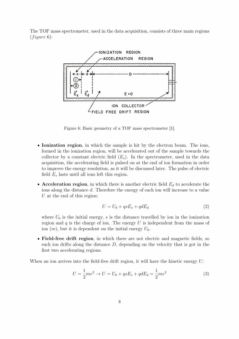
The TOF mass spectrometer, used in the data acquisition, consists of three main regions(figure 6):

Figure 6: Basic geometry of a TOF mass spectrometer [1].

Ionization region, in which the sample is hit by the electron beam. The ions,formed in the ionization region, will be accelerated out of the sample towards thecollector by a constant electric field (Es). In the spectrometer, used in the dataacquisition, the accelerating field is pulsed on at the end of ion formation in orderto improve the energy resolution, as it will be discussed later. The pulse of electricfield Es lasts until all ions left this region.

Acceleration region, in which there is another electric field Ed to accelerate theions along the distance d. Therefore the energy of each ion will increase to a valueU at the end of this region:

U = U0 + qsEs + qdEd (2)

where U0 is the initial energy, s is the distance travelled by ion in the ionizationregion and q is the charge of ion. The energy U is independent from the mass ofion (m), but it is dependent on the initial energy U0.

Field-free drift region, in which there are not electric and magnetic fields, soeach ion drifts along the distance D, depending on the velocity that is got in thefirst two accelerating regions.

When an ion arrives into the field-free drift region, it will have the kinetic energy U :

U =1

2mv2 → U = U0 + qsEs + qdEd =

1

2mv2 (3)

8

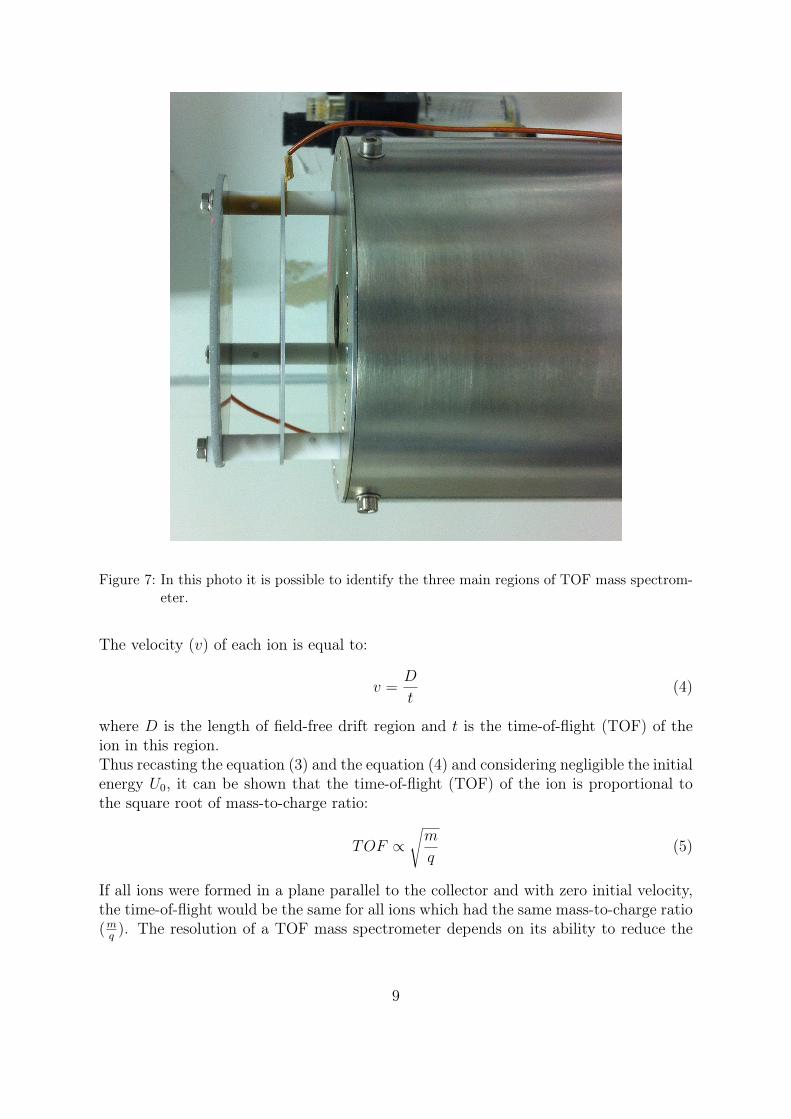
Figure 7: In this photo it is possible to identify the three main regions of TOF mass spectrom-eter.

The velocity (v) of each ion is equal to:

v =D

t(4)

where D is the length of field-free drift region and t is the time-of-flight (TOF) of theion in this region.Thus recasting the equation (3) and the equation (4) and considering negligible the initialenergy U0, it can be shown that the time-of-flight (TOF) of the ion is proportional tothe square root of mass-to-charge ratio:

TOF ∝√m

q(5)

If all ions were formed in a plane parallel to the collector and with zero initial velocity,the time-of-flight would be the same for all ions which had the same mass-to-charge ratio(mq). The resolution of a TOF mass spectrometer depends on its ability to reduce the

9

energy spread and the spatial distribution of the initial ion cloud. [1]

In the 1955 W.C.Wiley and I.H.McLaren developed a clever method to improve theenergy spread compensation, introducing a time-lag between the formation of ions andthe application of the first acceleration pulse (in this case, Es). During the time-lag, ionsmove to a new position because of their initial velocities, so the arrival time spread dueto initial kinetic energy differences is eliminated under proper experimental conditions.The TOF mass spectrometer, used for the data acquisition, is based exactly on time-lagprinciple.

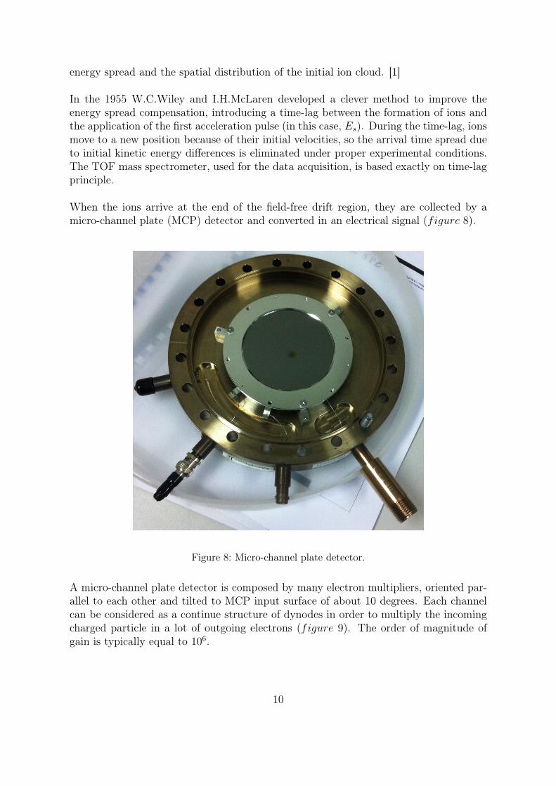
When the ions arrive at the end of the field-free drift region, they are collected by amicro-channel plate (MCP) detector and converted in an electrical signal (figure 8).

Figure 8: Micro-channel plate detector.

A micro-channel plate detector is composed by many electron multipliers, oriented par-allel to each other and tilted to MCP input surface of about 10 degrees. Each channelcan be considered as a continue structure of dynodes in order to multiply the incomingcharged particle in a lot of outgoing electrons (figure 9). The order of magnitude ofgain is typically equal to 106.

10

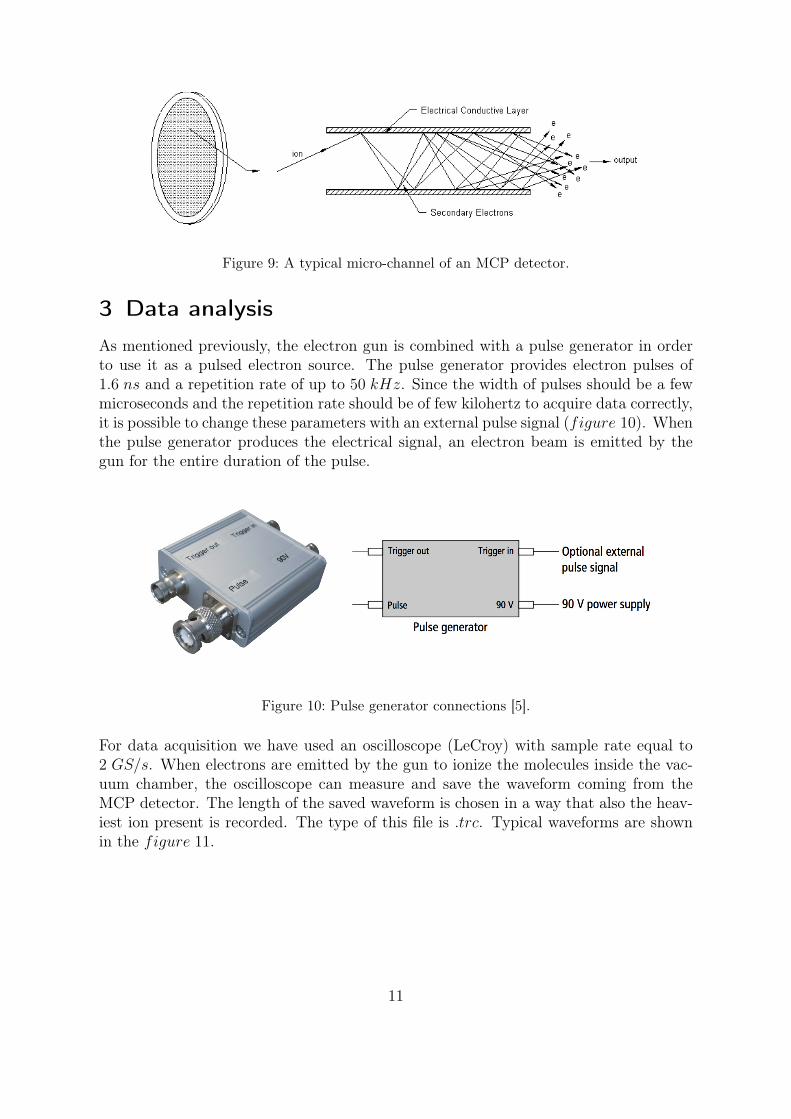
Figure 9: A typical micro-channel of an MCP detector.

3 Data analysis

As mentioned previously, the electron gun is combined with a pulse generator in orderto use it as a pulsed electron source. The pulse generator provides electron pulses of1.6 ns and a repetition rate of up to 50 kHz. Since the width of pulses should be a fewmicroseconds and the repetition rate should be of few kilohertz to acquire data correctly,it is possible to change these parameters with an external pulse signal (figure 10). Whenthe pulse generator produces the electrical signal, an electron beam is emitted by thegun for the entire duration of the pulse.

Figure 10: Pulse generator connections [5].

For data acquisition we have used an oscilloscope (LeCroy) with sample rate equal to2 GS/s. When electrons are emitted by the gun to ionize the molecules inside the vac-uum chamber, the oscilloscope can measure and save the waveform coming from theMCP detector. The length of the saved waveform is chosen in a way that also the heav-iest ion present is recorded. The type of this file is .trc. Typical waveforms are shownin the figure 11.

11

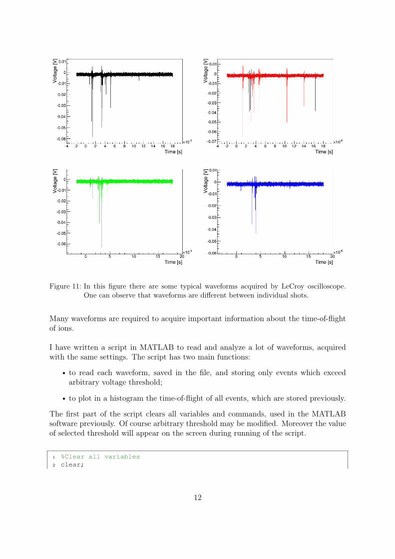
Figure 11: In this figure there are some typical waveforms acquired by LeCroy oscilloscope.One can observe that waveforms are different between individual shots.

Many waveforms are required to acquire important information about the time-of-flightof ions.

I have written a script in MATLAB to read and analyze a lot of waveforms, acquiredwith the same settings. The script has two main functions:

to read each waveform, saved in the file, and storing only events which exceedarbitrary voltage threshold;

to plot in a histogram the time-of-flight of all events, which are stored previously.

The first part of the script clears all variables and commands, used in the MATLABsoftware previously. Of course arbitrary threshold may be modified. Moreover the valueof selected threshold will appear on the screen during running of the script.

1 %Clear all variables2 clear;

12

3 clc;4

5 %Set the threshold to select the interesting events only6 threshold = -0.008;7 disp( strcat('Threshold: ', num2str(threshold), ' V') )

After setting some important variables, as for example the number of histogram´s bins(nbins), the function ReadLeCroyBinaryWaveform is called for each file inside the se-lected folder. The code of this function can be viewed on the Internet: [9]http://www.mathworks.com/matlabcentral/fileexchange/2114-readlecroybinarywaveform-m/content/ReadLeCroyBinaryWaveform.m.

The return value of this function is a record containing four elements:

ans.info: some information about waveform, for example oscilloscope ID, samplingtime and other settings;

ans.desc: in our case, this element is empty;

ans.y : voltage values sampled by the oscilloscope;

ans.x : array of time values corresponding to ans.y. It is important to underlinethat the time ”0” marks the trigger event (in our case, the leading edge of pulse).

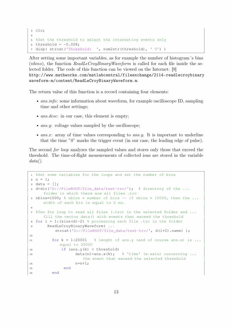
The second for loop analyzes the sampled values and stores only those that exceed thethreshold. The time-of-flight measurements of collected ions are stored in the variabledata().

1 %Set some variables for the loops and set the number of bins2 n = 1;3 data = [];4 d=dir('D://FileROOT/file_data/test-trc/'); % directory of the ...

folder in which there are all files .trc5 nbins=1000; % nbins = number of bins -- if nbins = 10000, then the ...

width of each bin is equal to 2 ns.6

7 %Two for loop to read all files (.trc) in the selected folder and ...fill the vector data() with events that exceed the threshold

8 for i = 1:(size(d)-2) % processing each file .trc in the folder9 ReadLeCroyBinaryWaveform( ...

strcat('D://FileROOT/file_data/test-trc/', d(i+2).name) );10

11 for k = 1:20001 % lenght of ans.y (and of course ans.x) is ...equal to 20000

12 if (ans.y(k) < threshold)13 data(n)=ans.x(k); % 'time' (x-axis) concerning ...

the event that exceed the selected threshold14 n=n+1;15 end16 end

13

17

18 %Clear the ans.x and ans.y, corresponding to the previous event19 clear ans.x20 clear ans.y21 end

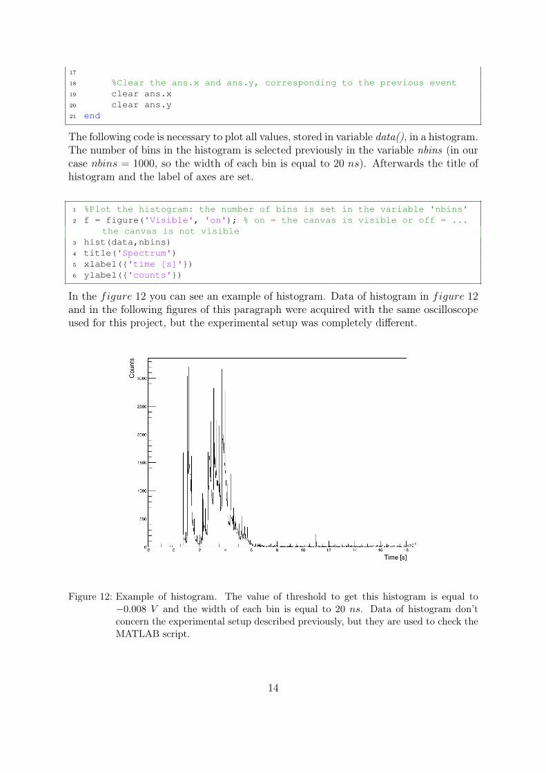
The following code is necessary to plot all values, stored in variable data(), in a histogram.The number of bins in the histogram is selected previously in the variable nbins (in ourcase nbins = 1000, so the width of each bin is equal to 20 ns). Afterwards the title ofhistogram and the label of axes are set.

1 %Plot the histogram: the number of bins is set in the variable 'nbins'2 f = figure('Visible', 'on'); % on = the canvas is visible or off = ...

the canvas is not visible3 hist(data,nbins)4 title('Spectrum')5 xlabel({'time [s]'})6 ylabel({'counts'})

In the figure 12 you can see an example of histogram. Data of histogram in figure 12and in the following figures of this paragraph were acquired with the same oscilloscopeused for this project, but the experimental setup was completely different.

Figure 12: Example of histogram. The value of threshold to get this histogram is equal to−0.008 V and the width of each bin is equal to 20 ns. Data of histogram don’tconcern the experimental setup described previously, but they are used to check theMATLAB script.

14

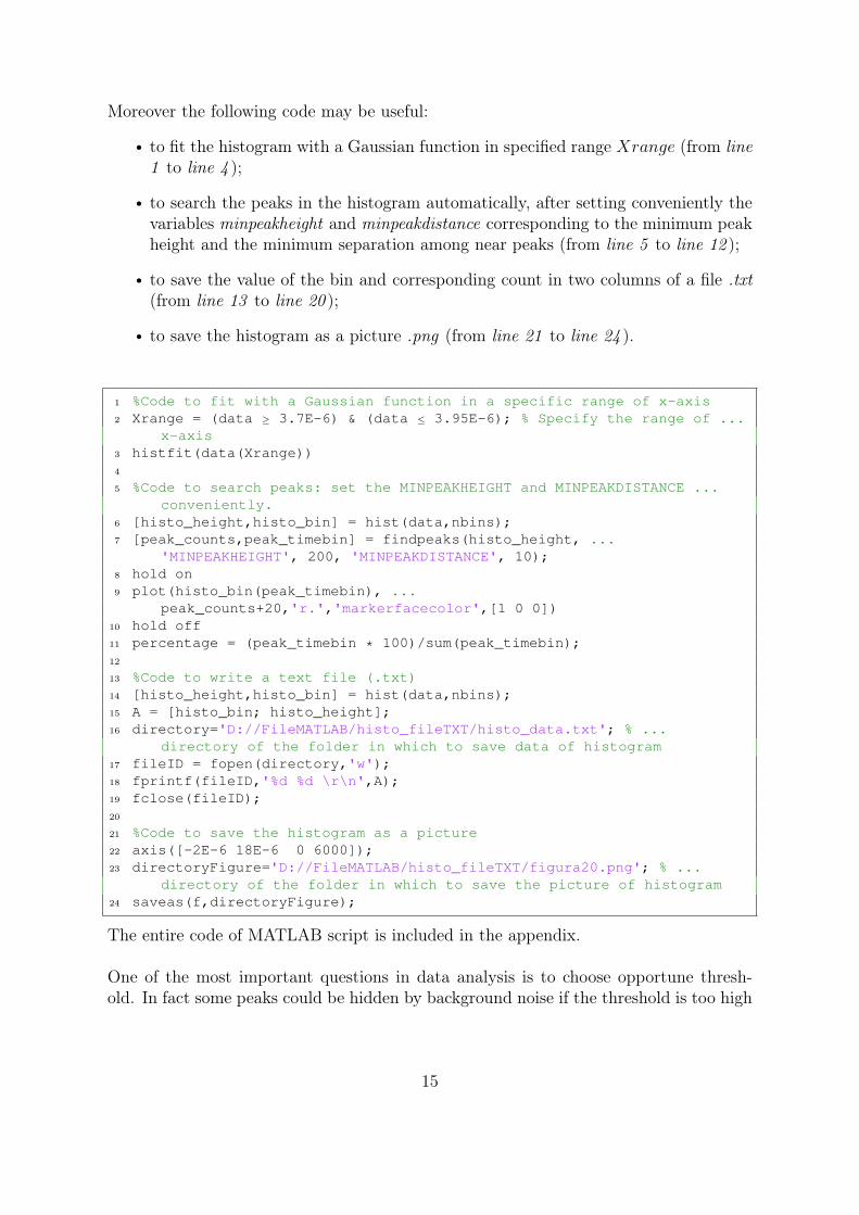
Moreover the following code may be useful:

to fit the histogram with a Gaussian function in specified range Xrange (from line1 to line 4 );

to search the peaks in the histogram automatically, after setting conveniently thevariables minpeakheight and minpeakdistance corresponding to the minimum peakheight and the minimum separation among near peaks (from line 5 to line 12 );

to save the value of the bin and corresponding count in two columns of a file .txt(from line 13 to line 20 );

to save the histogram as a picture .png (from line 21 to line 24 ).

1 %Code to fit with a Gaussian function in a specific range of x-axis2 Xrange = (data ≥ 3.7E-6) & (data ≤ 3.95E-6); % Specify the range of ...

x-axis3 histfit(data(Xrange))4

5 %Code to search peaks: set the MINPEAKHEIGHT and MINPEAKDISTANCE ...conveniently.

6 [histo_height,histo_bin] = hist(data,nbins);7 [peak_counts,peak_timebin] = findpeaks(histo_height, ...

'MINPEAKHEIGHT', 200, 'MINPEAKDISTANCE', 10);8 hold on9 plot(histo_bin(peak_timebin), ...

peak_counts+20,'r.','markerfacecolor',[1 0 0])10 hold off11 percentage = (peak_timebin * 100)/sum(peak_timebin);12

13 %Code to write a text file (.txt)14 [histo_height,histo_bin] = hist(data,nbins);15 A = [histo_bin; histo_height];16 directory='D://FileMATLAB/histo_fileTXT/histo_data.txt'; % ...

directory of the folder in which to save data of histogram17 fileID = fopen(directory,'w');18 fprintf(fileID,'%d %d \r\n',A);19 fclose(fileID);20

21 %Code to save the histogram as a picture22 axis([-2E-6 18E-6 0 6000]);23 directoryFigure='D://FileMATLAB/histo_fileTXT/figura20.png'; % ...

directory of the folder in which to save the picture of histogram24 saveas(f,directoryFigure);

The entire code of MATLAB script is included in the appendix.

One of the most important questions in data analysis is to choose opportune thresh-old. In fact some peaks could be hidden by background noise if the threshold is too high

15

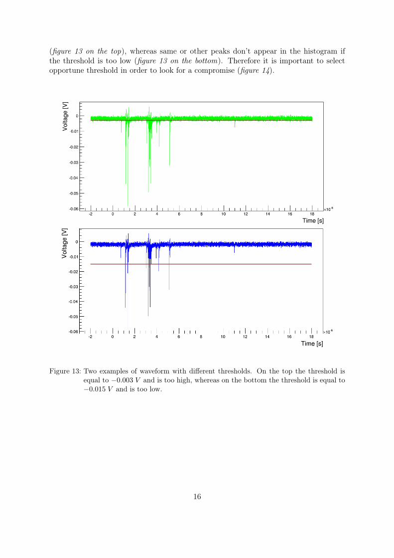
(figure 13 on the top), whereas same or other peaks don’t appear in the histogram ifthe threshold is too low (figure 13 on the bottom). Therefore it is important to selectopportune threshold in order to look for a compromise (figure 14).

Figure 13: Two examples of waveform with different thresholds. On the top the threshold isequal to −0.003 V and is too high, whereas on the bottom the threshold is equal to−0.015 V and is too low.

16

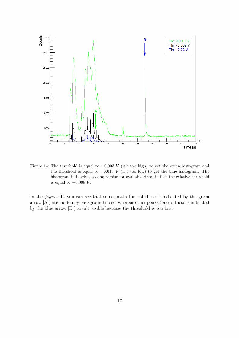
Figure 14: The threshold is equal to −0.003 V (it’s too high) to get the green histogram andthe threshold is equal to −0.015 V (it’s too low) to get the blue histogram. Thehistogram in black is a compromise for available data, in fact the relative thresholdis equal to −0.008 V .

In the figure 14 you can see that some peaks (one of these is indicated by the greenarrow [A]) are hidden by background noise, whereas other peaks (one of these is indicatedby the blue arrow [B]) aren’t visible because the threshold is too low.

17

4 Results and discussion

The most important purpose of this project is to characterize the electron source inorder to identify the best parameters for electron ionization inside the vacuum chamber.Other purposes of this project may be:

to verify the correctness of data measurements, for example to prove the repeata-bility of data measurements and to check that the time-of-flight of ions is reallyproportional to the square root of mass-to-charge ratio (TOF ∝

√mq);

to measure some ionization energies of argon gas and to compare them with otherand independent values, for example with the values of National Institute forStandards and Technologies (NIST) [10]. It is important to underline that theenergy range of electron beam is about 100 − 4000 eV (more information in theparagraph 2.2), so only a few ionization energies will be possible to measure;

to measure the energy resolution of time-of-flight mass spectrometer on varyingof some parameters, for example wehnelt voltage, focus voltage, pressure insidevacuum chamber, etc.

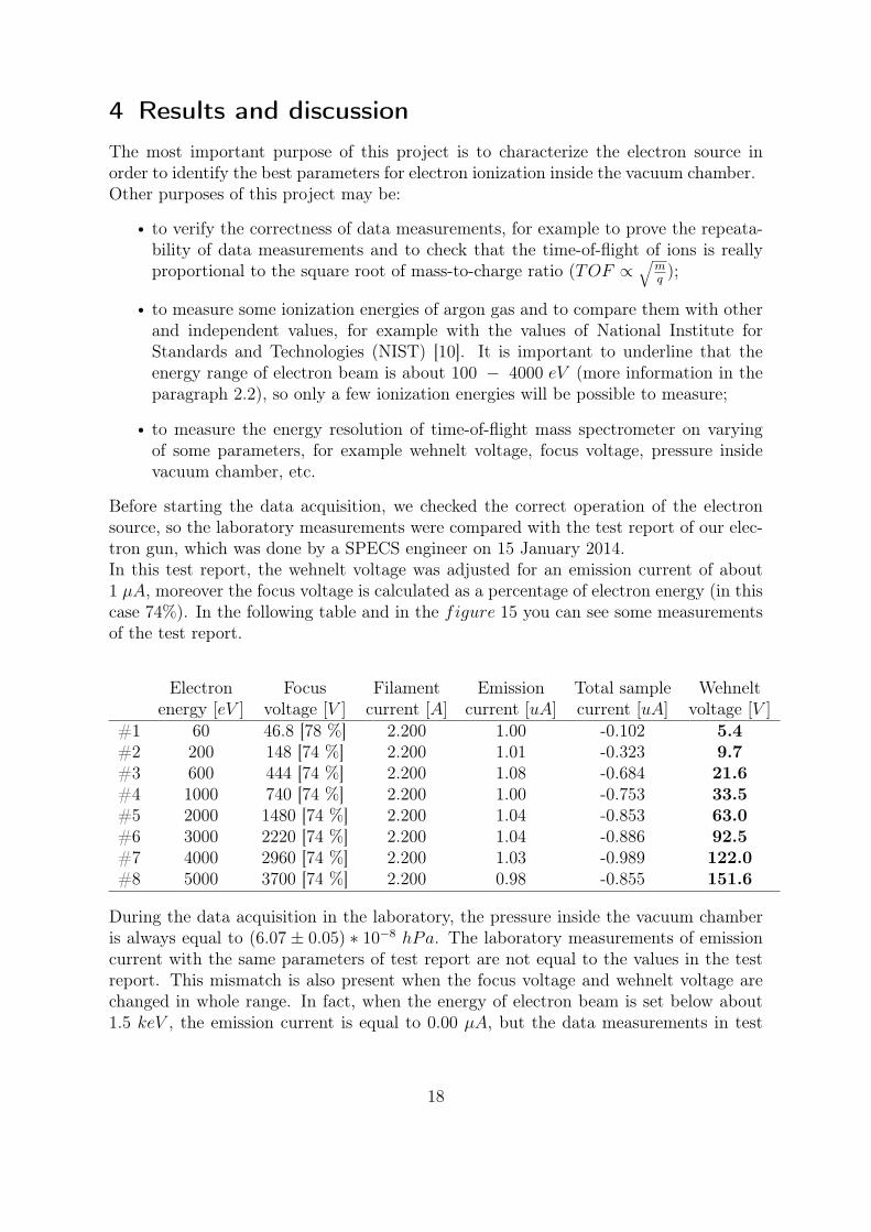
Before starting the data acquisition, we checked the correct operation of the electronsource, so the laboratory measurements were compared with the test report of our elec-tron gun, which was done by a SPECS engineer on 15 January 2014.In this test report, the wehnelt voltage was adjusted for an emission current of about1 µA, moreover the focus voltage is calculated as a percentage of electron energy (in thiscase 74%). In the following table and in the figure 15 you can see some measurementsof the test report.

Electron Focus Filament Emission Total sample Wehneltenergy [eV ] voltage [V ] current [A] current [uA] current [uA] voltage [V ]

#1 60 46.8 [78 %] 2.200 1.00 -0.102 5.4#2 200 148 [74 %] 2.200 1.01 -0.323 9.7#3 600 444 [74 %] 2.200 1.08 -0.684 21.6#4 1000 740 [74 %] 2.200 1.00 -0.753 33.5#5 2000 1480 [74 %] 2.200 1.04 -0.853 63.0#6 3000 2220 [74 %] 2.200 1.04 -0.886 92.5#7 4000 2960 [74 %] 2.200 1.03 -0.989 122.0#8 5000 3700 [74 %] 2.200 0.98 -0.855 151.6

During the data acquisition in the laboratory, the pressure inside the vacuum chamberis always equal to (6.07 ± 0.05) ∗ 10−8 hPa. The laboratory measurements of emissioncurrent with the same parameters of test report are not equal to the values in the testreport. This mismatch is also present when the focus voltage and wehnelt voltage arechanged in whole range. In fact, when the energy of electron beam is set below about1.5 keV , the emission current is equal to 0.00 µA, but the data measurements in test

18

report are completely different. Instead if the energy of electron beam is set above moreor less 1.5 keV , there are a lot of fluctuations of emission current: in fact this valuechanges in the entire range (0 − 250 µA) rapidly, without ever becoming stable. Thereare also a lot of fluctuations of electron energy.

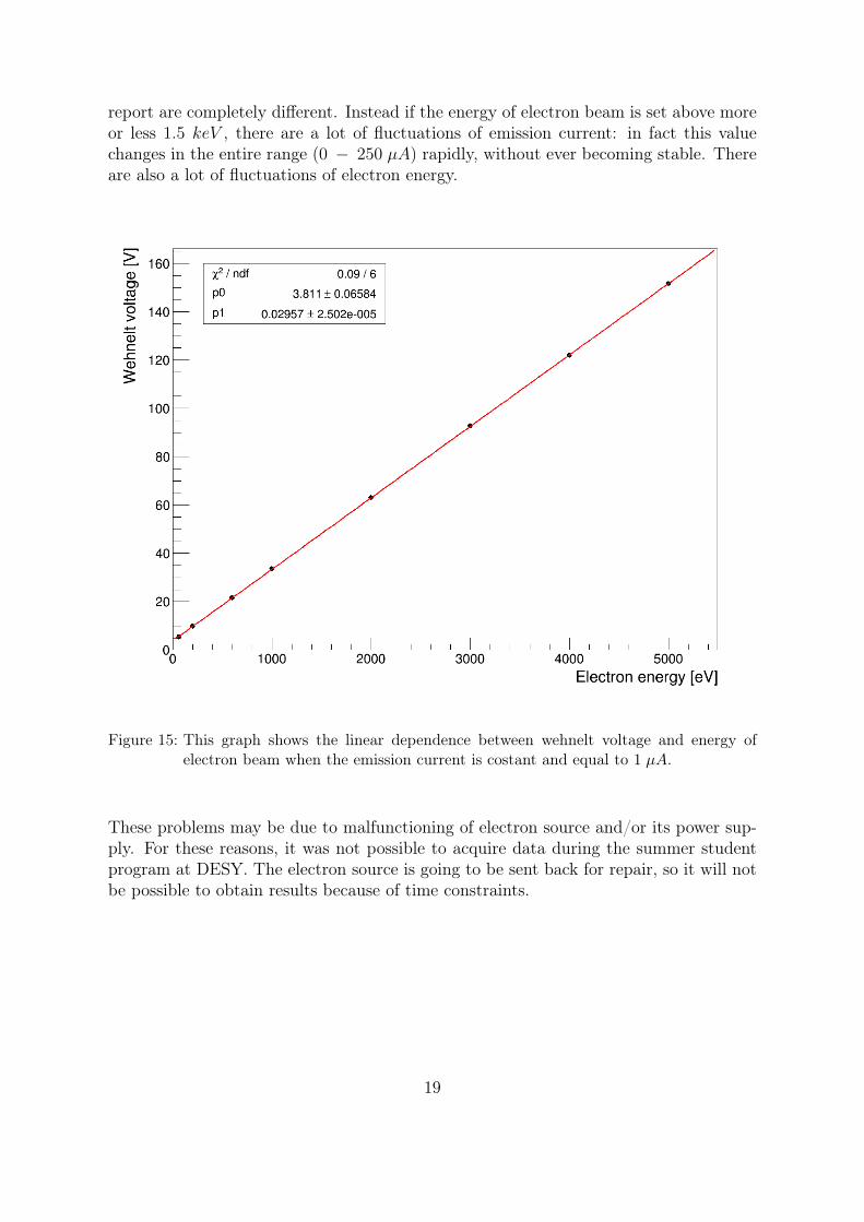
Figure 15: This graph shows the linear dependence between wehnelt voltage and energy ofelectron beam when the emission current is costant and equal to 1 µA.

These problems may be due to malfunctioning of electron source and/or its power sup-ply. For these reasons, it was not possible to acquire data during the summer studentprogram at DESY. The electron source is going to be sent back for repair, so it will notbe possible to obtain results because of time constraints.

19

5 Conclusions

The apparatus for data measurements is assembled, so all devices are adjusted and allelectronic connections are plugged. The pressure inside the vacuum chamber reaches thedesired value (< 10−6 hPa).A MATLAB script was written to analyse the waveforms coming from the time-of-flightmass spectrometer, in fact it is important to select the signals of ions from noise.During the summer student program at DESY, it was not possible to acquire datameasurements and to identify the best parameters for electron ionization because theelectron source does not operate correctly, so it absolutely needs to be repaired.

20

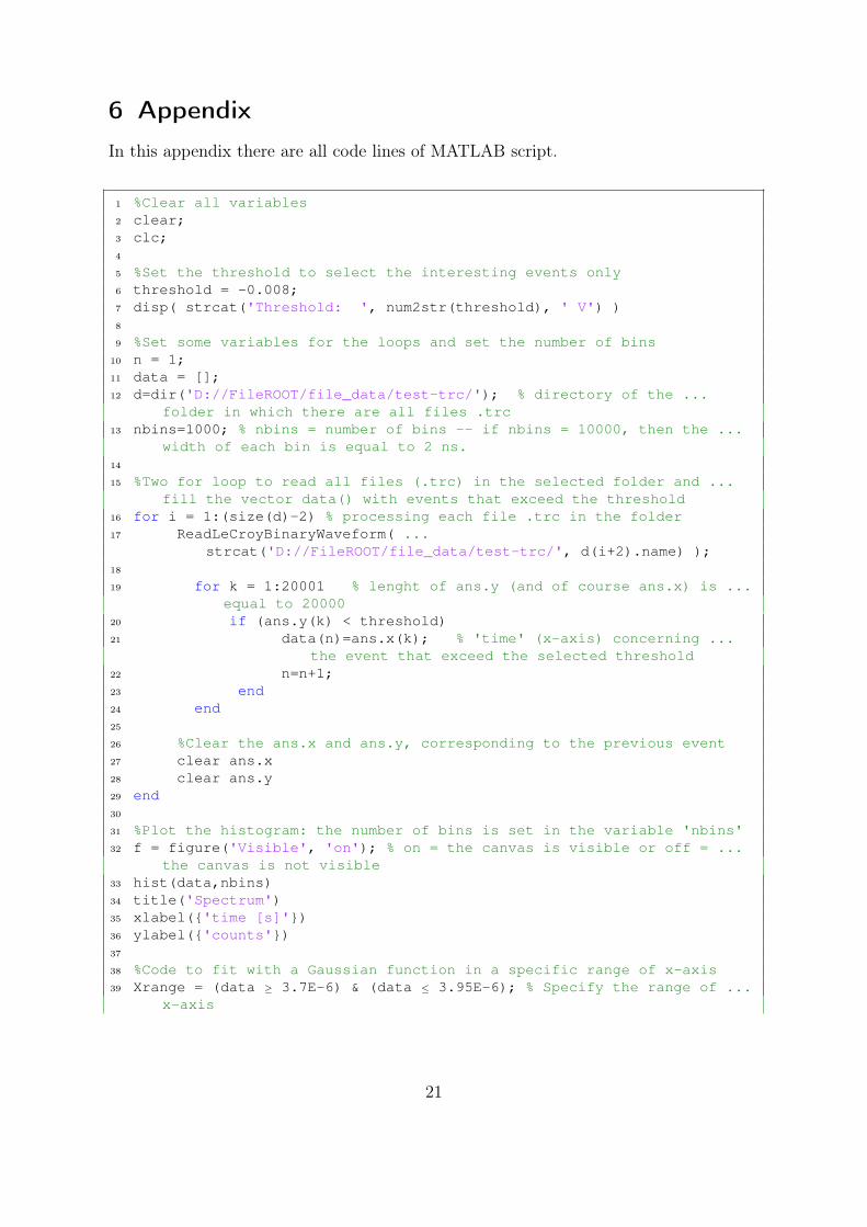
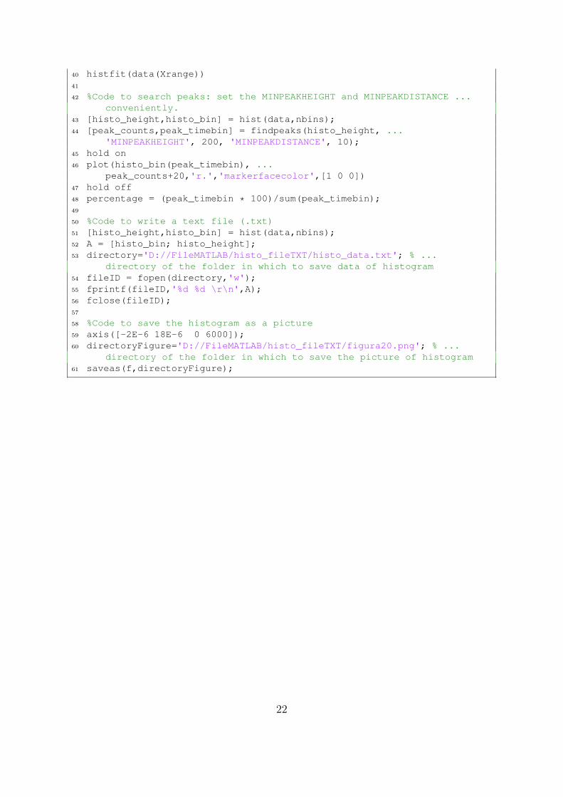
6 Appendix

In this appendix there are all code lines of MATLAB script.

1 %Clear all variables2 clear;3 clc;4

5 %Set the threshold to select the interesting events only6 threshold = -0.008;7 disp( strcat('Threshold: ', num2str(threshold), ' V') )8

9 %Set some variables for the loops and set the number of bins10 n = 1;11 data = [];12 d=dir('D://FileROOT/file_data/test-trc/'); % directory of the ...

folder in which there are all files .trc13 nbins=1000; % nbins = number of bins -- if nbins = 10000, then the ...

width of each bin is equal to 2 ns.14

15 %Two for loop to read all files (.trc) in the selected folder and ...fill the vector data() with events that exceed the threshold

16 for i = 1:(size(d)-2) % processing each file .trc in the folder17 ReadLeCroyBinaryWaveform( ...

strcat('D://FileROOT/file_data/test-trc/', d(i+2).name) );18

19 for k = 1:20001 % lenght of ans.y (and of course ans.x) is ...equal to 20000

20 if (ans.y(k) < threshold)21 data(n)=ans.x(k); % 'time' (x-axis) concerning ...

the event that exceed the selected threshold22 n=n+1;23 end24 end25

26 %Clear the ans.x and ans.y, corresponding to the previous event27 clear ans.x28 clear ans.y29 end30

31 %Plot the histogram: the number of bins is set in the variable 'nbins'32 f = figure('Visible', 'on'); % on = the canvas is visible or off = ...

the canvas is not visible33 hist(data,nbins)34 title('Spectrum')35 xlabel({'time [s]'})36 ylabel({'counts'})37

38 %Code to fit with a Gaussian function in a specific range of x-axis39 Xrange = (data ≥ 3.7E-6) & (data ≤ 3.95E-6); % Specify the range of ...

x-axis

21

40 histfit(data(Xrange))41

42 %Code to search peaks: set the MINPEAKHEIGHT and MINPEAKDISTANCE ...conveniently.

43 [histo_height,histo_bin] = hist(data,nbins);44 [peak_counts,peak_timebin] = findpeaks(histo_height, ...

'MINPEAKHEIGHT', 200, 'MINPEAKDISTANCE', 10);45 hold on46 plot(histo_bin(peak_timebin), ...

peak_counts+20,'r.','markerfacecolor',[1 0 0])47 hold off48 percentage = (peak_timebin * 100)/sum(peak_timebin);49

50 %Code to write a text file (.txt)51 [histo_height,histo_bin] = hist(data,nbins);52 A = [histo_bin; histo_height];53 directory='D://FileMATLAB/histo_fileTXT/histo_data.txt'; % ...

directory of the folder in which to save data of histogram54 fileID = fopen(directory,'w');55 fprintf(fileID,'%d %d \r\n',A);56 fclose(fileID);57

58 %Code to save the histogram as a picture59 axis([-2E-6 18E-6 0 6000]);60 directoryFigure='D://FileMATLAB/histo_fileTXT/figura20.png'; % ...

directory of the folder in which to save the picture of histogram61 saveas(f,directoryFigure);

22

References

[1] W.C.Wiley and I.H.McLaren (1955), Time-of-Flight Mass Spectrometer with Im-proved Resolution, The review of scientific instruments, vol. 26, no. 12, pp. 1150-1157

[2] D.S.Belic, J.Lecointre and P.Defrance (2010), Electron impact multiple ionizationof argon ions, J. Phys. B: At. Mol. Opt. Phys. 43 185203 (10pp)

[3] H. C. Straub, P. Renault, B. G. Lindsay, K. A. Smith, and R. F. Stebbings (1995),Absolute partial and total cross sections for electron-impact ionization of argon fromthreshold to 1000 eV, Physical Review A, vol. 52, no. 2, pp. 1115-1124

[4] Manual of electron source, Specs EQ 22/35, version 1.0

[5] EQ 22 pulsed electron source - application note, Specs EQ 22/35, version 1.0

[6] http://en.wikipedia.org/wiki/Einzel_lens

[7] http://en.wikipedia.org/wiki/Electron_gun

[8] http://www.photonis.com/attachment.php?id_attachment=142

[9] http://www.mathworks.com/matlabcentral/fileexchange/2114-readlecroybinarywaveform-m/content/ReadLeCroyBinaryWaveform.m

[10] http://physics.nist.gov/cgi-bin/ASD/ie.pl?spectra=Ar&units=1&at_num_out=on&el_name_out=on&seq_out=on&shells_out=on&level_out=on&e_out=0&unc_out=on&biblio=on

23