Chapter 5Risk-Aversion, Capital Asset Allocation, and MarkowitzPortfolio-Selection Model

Cheng-Few Lee, Joseph E. Finnerty, and Hong-Yi Chen

Abstract In this chapter, we first introduce utility functionand indifference curve. Based on utility theory, we derive theMarkowitz’s model and the efficient frontier through the cre-ation of efficient portfolios of varying risk and return. Wealso include methods of solving for the efficient frontier bothgraphically and mathematically, with and without explicitlyincorporating short selling.

Keywords Markowitz model � Utility theory � Utility func-tions � Indifference curve � Risk averse � Short selling � Dylmodel � Iso-return line � Iso-variance ellipse � Critical line �

Lagrange multipliers

5.1 Introduction

In this chapter, we address basic portfolio analysis conceptsand techniques discussed in the Markowitz portfolio-selection model and other related issues in portfolio anal-ysis. Before Harry Markowitz (1952, 1959) developed hisportfolio-selection technique into what is now modern port-folio theory (MPT), security-selection models focused pri-marily on the returns generated by investment opportunities.The Markowitz theory retained the emphasis on return, but itelevated risk to a coequal level of importance, and the con-cept of portfolio risk was born. Whereas risk had been con-sidered an important factor and variance an accepted way ofmeasuring risk, Markowitz was the first to clearly and rigor-ously show how the variance of a portfolio can be reducedthrough the impact of diversification. He demonstrated thatby combining securities that are not perfectly positively cor-related into a portfolio, the portfolio variance can be reduced.

The Markowitz model is based on several assumptionsconcerning the behavior of investors:

H.-Y. Chen (�) and C.-F. LeeRutgers University, New Brunswick, NJ, USAe-mail: hchen37@pegasus.rutgers.edu

J.E. FinnertyUniversity of Illinois, Urbana-Champaign, IL, USAe-mail: finnerty@illinois.edu

1. A probability distribution of possible returns over someholding period can be estimated by investors.

2. Investors have single-period utility functions in whichthey maximize utility within the framework of diminish-ing marginal utility of wealth.

3. Variability about the possible values of return is used byinvestors to measure risk.

4. Investors use only expected return and risk to makeinvestment decisions.

5. Expected return and risk as used by investors are mea-sured by the first two moments of the probability distribu-tion of returns-expected value and variance.

6. Return is desirable; risk is to be avoided.

It follows, then, that a security or portfolio is considered effi-cient if there is no other investment opportunity with a higherlevel of return at a given level of risk and no other opportu-nity with a lower level of risk at a given level of return.

5.2 Measurement of Return and Risk

This section focuses on the return and risk measurementsutilized in applying the Markowitz model to efficient port-folio selection.

5.2.1 Return

Using the probability distribution of expected returns for aportfolio, investors are assumed to measure the level of returnby computing the expected value of the distribution.

E.RP/ DnX

iD1WiE .Ri/ (5.1)

where:nX

iD1Wi D 1:0I

C.-F. Lee et al. (eds.), Handbook of Quantitative Finance and Risk Management,DOI 10.1007/978-0-387-77117-5_5, c� Springer Science+Business Media, LLC 2010

69

70 C.-F. Lee et al.

n D the number of securities;Wi D the proportion of the funds invested in security i ;Ri, RP D the return on i th security and portfolio p; andE . / D the expectation of the variable in the parentheses.

Thus, the return computation is nothing more than findingthe weighted average return of the securities included in theportfolio. The risk measurement to be discussed in the nextsection is not quite so simple, however. For only in the caseof perfect positive correlation among all its components isthe standard deviation of the portfolio equal to the weightedaverage standard deviation of its component securities.

5.2.2 Risk

Risk is assumed to be measurable by the variability aroundthe expected value of the probability distribution of returns.The most accepted measures of this variability are the vari-ance and standard deviation. The variance of a single secu-rity is the expected value of the sum of the squared deviationsfrom the mean, and the standard deviation is the square rootof the variance. The variance of a portfolio combination ofsecurities is equal to the weighted average covariance of thereturns on its individual securities:

Var�Rp� D

nX

iD1

nX

jD1WiWjCov

�Ri ;Rj

�(5.2)

Covariance can also be expressed in terms of the correlationcoefficient as follows:

Cov�Ri ;Rj

� D rij �i �j D �ij (5.3)

Where rij D correlation coefficient between the rates of re-turn on security i; Ri , and the rates of return on securityj; Rj , and �i , and �j represent standard deviations of Riand Rj respectively. Therefore:

Var�Rp� D

nX

iD1

nX

jD1WiWj rij �i�j (5.4)

For a portfolio with two securities, A and B, the followingexpression can be developed:

Var�Rp� D

BX

iDA

BX

jDAWiWj rij �i �j

D WAWArAA�A�A CWAWBrAB�A�B

CWBWArBA�B�A CWBWBrBB�B�B

Since rAA and rBB D 1:0 by definition, terms can be simpli-fied and rearranged, yielding:

Var�Rp� D W 2

A�2A

CW 2B�2B

C 2WAWBrAB�A�B (5.5)

For a three-security portfolio, the variance of portfolio canbe defined:

Var�Rp� D

CPiDA

CPjDA

WiWj rij �i�j

D WAWArAA�A�A CWAWBrAB�A�BCWAWCrAC�A�C CWBWArAB�B�ACWBWBrBB�B�B CWBWCrBC�B�CCWCWArCA�C�A CWCWBrCB�C �BCWCWCrCC�C�C

Again simplifying and rearranging yields:

Var�Rp� D W 2

A�2A

CW 2B�2B

CW 2C�2C

C 2.WAWBrAB�A�BCWAWCrAC�A�C CWBWC rBC�B�C /

(5.6)

Thus, as the number of securities increases from three totwo, there is one more variance term and two more covari-ance terms. The general formula for determining the numberof terms that must be computed (NTC) to determine the vari-ance of a portfolio with N securities is

NTC D N variancesCN2 �N2

covariances

For the two-security example two variances were involved�2A

and �2B

, and�22 � 2

�ı2 D .4 � 2/=2 D 1 covariances,

�AB, or three computations. For the three-security case, threevariances and

�32 � 3�ı2 D .9 � 3/=2 D 3 covariances

were needed, �AB; �AC , and �BC, or six computations. Withfour securities, the total number would be 4C �

42 � 4�ı2 D

4C .16 � 4/=2 D 4C 6 D 10 computations. As shown fromthese examples, the number of covariance terms increases byN � 1, and the number of variance terms increases by one,as N increases by 1 unit.

If rAB D rAC D rBC D 1, then the securities are perfectlypositively correlated with each other, and Equation (5.6)reduces to:

Var�Rp� D .WA�A CWB�B CWC�C /

2 (5:60)

This implies that the standard deviation of the portfolio isequal to the weighted average standard deviation of its com-ponent securities. In other words:

Standard deviation of Rp D WA�A CWB�B CWC�C

5 Risk-Aversion, Capital Asset Allocation, and Markowitz Portfolio-Selection Model 71

Table 5.1 Portfolio size and variance computationsNumber of securities Number of Var and Cov terms

2 3

3 6

4 10

5 15

10 55

15 120

20 210

25 325

50 1; 275

75 2; 850

100 5; 050

250 31; 375

500 125; 250

Table 5.1 clearly illustrates the tremendous estimation andcomputational load that exists using the Markowitz diversifi-cation approach. Later chapters will illustrate how this prob-lem can be alleviated.

5.3 Utility Theory, Utility Functions,and Indifference Curves

In this section, utility theory and functions, which are neededfor portfolio analysis and capital asset models, will be dis-cussed in detail.

Utility theory is the foundation for the theory of choiceunder uncertainty. Following Henderson and Quandt (1980),cardinal and ordinal theories are the two major alternativesused by economists to determine how people and societieschoose to allocate scarce resources and to distribute wealthamong one another over time.1

5.3.1 Utility Functions

Economists define the relationships between psychologicalsatisfaction and wealth as “utility.” An upward-sloping rela-tionship, as shown in Fig. 5.1, identifies the phenomena of in-creasing wealth and increasing satisfaction as being directlyrelated. These relationships can be classified into linear, con-cave, and convex utility functions.

1 A cardinal utility implies that a consumer is capable of assigning toevery commodity or combination of commodities a number represent-ing the amount or degree of utility associated with it. An ordinary utilityimplies that a consumer needs not be able to assign numbers that rep-resent (in arbitrary unit) the degree or amount of utility associated withcommodity or combination of commodity. The consumer can only rankand order the amount or degree of utility associated with commodity.

In Fig. 5.1a, for each unit change in wealth, there is alinear utility function and equal increase in satisfaction orutility. A doubling of wealth will double satisfaction, and soon. If an investor’s utility function is a linear utility function,we call this kind of investor a risk-neutral investor. This isprobably not very realistic: a dollar increase in wealth from$2 to $1 is probably more important than an increase from $2million to $1 million, because the marginal utility diminisheswith increased wealth.

In Fig. 5.1b the concave utility function shows the rela-tionship of an increase in wealth and a less-than-proportionalincrease in utility. In other words, the marginal utility ofwealth decreases as wealth increases. As mentioned above,the $1 increase from $2 to $1 of wealth is more important tothe individual than the increase from $1,000,001 to $1 mil-lion. Each successive increase in wealth adds less satisfactionas the level of wealth rises. We call an investor with a con-cave utility function a risk-averse investor.

Finally, Fig. 5.1c is a convex utility function, which de-notes a more than proportional increase in satisfaction foreach increase in wealth. Behaviorally, the richer you are themore satisfaction you receive in getting an additional dollarof wealth. Investors with convex utility functions are calledrisk-seeking investors.

The utility theory primarily used in finance is that de-veloped by Von Neumann and Morgenstern (VNM 1947).VNM define investor utility as a function of rates of returnor wealth. Mao (1969) points out that the VNM utility theoryis really somewhere between the cardinal and ordinal util-ity theories. The function associated with the VNM’s utilitytheory in terms of wealth can be defined:

U D f .�w; �w/

where �w indicates expected future wealth and �w representsthe predicted standard deviation of the possible divergence ofactual future wealth from �w.

Investors are expected to prefer a higher expected futurewealth to a lower value. Moreover, they are generally riskaverse as well. That is, they prefer a lower value of �w toa higher value, given the level of �w.2 These assumptionsimply that the indifference curves relating �w and �w willbe upward sloping, as indicated in Fig. 5.2. In Fig. 5.2, eachindifference curve is an expected utility isoquant showing allthe various combinations of risk and return that provide anequal amount of expected utility for the investor.

In explaining how investment decisions or portfoliochoices are made, utility theory is used here not to implythat individuals actually make decisions using a utility curve,but rather as an expository vehicle that helps explain how

2 Technically, these conditions can be represented mathematically by@U =@�w > 0 and @U =@�w < 0.

72 C.-F. Lee et al.

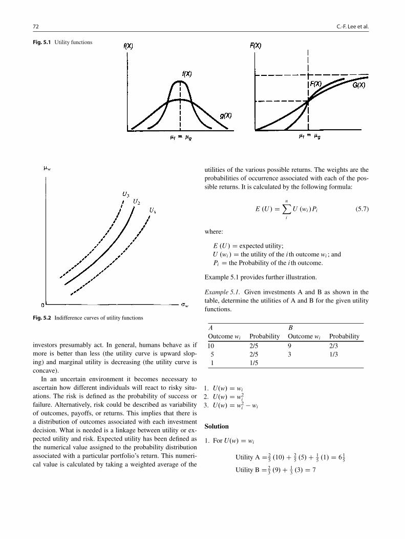
Fig. 5.1 Utility functions

Fig. 5.2 Indifference curves of utility functions

investors presumably act. In general, humans behave as ifmore is better than less (the utility curve is upward slop-ing) and marginal utility is decreasing (the utility curve isconcave).

In an uncertain environment it becomes necessary toascertain how different individuals will react to risky situ-ations. The risk is defined as the probability of success orfailure. Alternatively, risk could be described as variabilityof outcomes, payoffs, or returns. This implies that there isa distribution of outcomes associated with each investmentdecision. What is needed is a linkage between utility or ex-pected utility and risk. Expected utility has been defined asthe numerical value assigned to the probability distributionassociated with a particular portfolio’s return. This numeri-cal value is calculated by taking a weighted average of the

utilities of the various possible returns. The weights are theprobabilities of occurrence associated with each of the pos-sible returns. It is calculated by the following formula:

E .U / DnX

i

U .wi /Pi (5.7)

where:

E .U / D expected utility;U .wi / D the utility of the i th outcome wi ; andPi D the Probability of the i th outcome.

Example 5.1 provides further illustration.

Example 5.1. Given investments A and B as shown in thetable, determine the utilities of A and B for the given utilityfunctions.

A B

Outcome wi Probability Outcome wi Probability

10 2/5 9 2/35 2/5 3 1/31 1/5

1. U.w/ D wi2. U.w/ D w2i3. U.w/ D w2i � wi

Solution

1. For U.w/ D wi

Utility A D 25.10/C 2

5.5/C 1

5.1/ D 61

5

Utility B D 23.9/C 1

3.3/ D 7

5 Risk-Aversion, Capital Asset Allocation, and Markowitz Portfolio-Selection Model 73

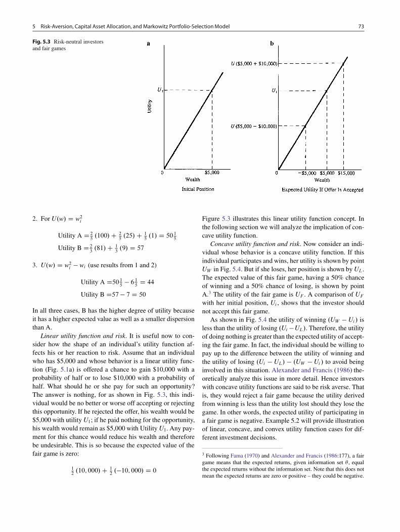
Fig. 5.3 Risk-neutral investorsand fair games

2. For U.w/ D w2i

Utility A D 25.100/C 2

5.25/C 1

5.1/ D 501

5

Utility B D 23.81/C 1

3.9/ D 57

3. U.w/ D w2i � wi (use results from 1 and 2)

Utility A D5015

� 615

D 44

Utility B D57� 7 D 50

In all three cases, B has the higher degree of utility becauseit has a higher expected value as well as a smaller dispersionthan A.

Linear utility function and risk. It is useful now to con-sider how the shape of an individual’s utility function af-fects his or her reaction to risk. Assume that an individualwho has $5,000 and whose behavior is a linear utility func-tion (Fig. 5.1a) is offered a chance to gain $10,000 with aprobability of half or to lose $10,000 with a probability ofhalf. What should he or she pay for such an opportunity?The answer is nothing, for as shown in Fig. 5.3, this indi-vidual would be no better or worse off accepting or rejectingthis opportunity. If he rejected the offer, his wealth would be$5,000 with utility U1; if he paid nothing for the opportunity,his wealth would remain as $5,000 with Utility U1. Any pay-ment for this chance would reduce his wealth and thereforebe undesirable. This is so because the expected value of thefair game is zero:

12.10; 000/C 1

2.�10; 000/ D 0

Figure 5.3 illustrates this linear utility function concept. Inthe following section we will analyze the implication of con-cave utility function.

Concave utility function and risk. Now consider an indi-vidual whose behavior is a concave utility function. If thisindividual participates and wins, her utility is shown by pointUW in Fig. 5.4. But if she loses, her position is shown by UL.The expected value of this fair game, having a 50% chanceof winning and a 50% chance of losing, is shown by pointA.3 The utility of the fair game is UF . A comparison of UFwith her initial position, Ui , shows that the investor shouldnot accept this fair game.

As shown in Fig. 5.4 the utility of winning .UW � Ui/ isless than the utility of losing .Ui �UL/. Therefore, the utilityof doing nothing is greater than the expected utility of accept-ing the fair game. In fact, the individual should be willing topay up to the difference between the utility of winning andthe utility of losing .Ui � UL/ � .UW � Ui/ to avoid beinginvolved in this situation. Alexander and Francis (1986) the-oretically analyze this issue in more detail. Hence investorswith concave utility functions are said to be risk averse. Thatis, they would reject a fair game because the utility derivedfrom winning is less than the utility lost should they lose thegame. In other words, the expected utility of participating ina fair game is negative. Example 5.2 will provide illustrationof linear, concave, and convex utility function cases for dif-ferent investment decisions.

3 Following Fama (1970) and Alexander and Francis (1986:177), a fairgame means that the expected returns, given information set � , equalthe expected returns without the information set. Note that this does notmean the expected returns are zero or positive – they could be negative.

74 C.-F. Lee et al.

E(UF)

E(Ul)

Uw-Ui =

Ui-UL =

Concave Utility Function

Linear Utility Function

For a risk-averse investor

\Reject a fair gameQUi > E (UF) Þ E(UF)-Ui < 0

Fig. 5.4 Risk-averse investors and fair games

E.UF / D 12.Uw C UL/ is the expected utility of the fair

game under a concave utility function.E.U`/ is the expected utility of the fair game under a lin-

ear utility function.

Example 5.2. Given the following utility functions for fourinvestors, what can you conclude about their reaction towardsa fair game?

1. u.w/ D w C 4

2. u.w/ D w � 12w2 (quadratic utility function)

3. u.w/ D �e�2w (negative exponential utility function), and4. u.w/ D w2 � 4w

Evaluate the second derivative of the utility functions accord-ing to the following rules.

u00

.w/ < 0 implies risk averseu

00

.w/ D 0 implies risk neutralu

00

.w/ > 0 implies risk seeker

Solution

1. u.w/ D w C 4

u0.w/ D 1

u00

.w/ D 0

This implies risk neutrality; it is indifference for the in-vestor to accept or reject a fair gamble.

2. u.w/ D w � 12w2

u0.w/ D �w2

u00

.w/ D �2w < 0.We assume wealth is nonnegative:/

This implies the investor is risk averse and would reject afair gamble.

3. u.w/ D �e�2w

u0.w/ D 2e�2w

u00

.w/ D �4e�2w < 0

This implies risk adversity; the investor would reject a fairgamble.

4. u.w/ D w2 � 4wu0.w/ D 2w � 4u

00

.w/ D 2 > 0

This implies risk preference; the investor would seek a fairgamble.

The convex utility function is not realistic in real-worlddecisions; therefore, it is not further explored at this point.The following section discusses the implications of alterna-tive utility functions in terms of indifference curves.

5.3.2 Risk Aversion and Utility Values

But when risk increases along with return, the most attractiveportfolio is not obvious. How can investors quantify the rateat which they are willing to trade off return against risk? Byassuming that each investor can assign a welfare, or utility,score to competing investment portfolios based on the ex-pected return and risk of those portfolios. Higher utility val-ues are assigned to portfolios with more attractive risk-return

5 Risk-Aversion, Capital Asset Allocation, and Markowitz Portfolio-Selection Model 75

profiles. Portfolios receive higher utility scores for higher ex-pected returns and lower scores for higher volatility.

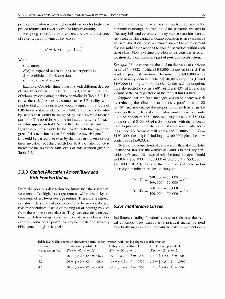
Assigning a portfolio with expected return and varianceof returns, the following utility score:

U D E.r/� 1

2A s2

Where

U D utilityE.r/ D expected return on the asset or portfolioA D coefficient of risk aversions2 D variance of returns

Example: Consider three investors with different degreesof risk aversion: A1 D 2:0; A2 D 3:0, and A3 D 4:0, allof whom are evaluating the three portfolios in Table 5.2. Be-cause the risk-free rate is assumed to be 5%, utility scoreimplies that all three investors would assign a utility score of0.05 to the risk-free alternative. Table 5.2 presents the util-ity scores that would be assigned by each investor to eachportfolio. The portfolio with the highest utility score for eachinvestor appears in bold. Notice that the high-risk portfolio,H, would be chosen only by the investor with the lowest de-gree of risk aversion, A1 D 2:0, while the low-risk portfolio,L. would be passed over even by the most risk-averse of ourthree investors. All three portfolios beat the risk-free alter-native for the investors with levels of risk aversion given inTable 5.2.

5.3.3 Capital Allocation Across Risky andRisk-Free Portfolios

From the previous discussion we know that the riskier in-vestments offer higher average returns, while less risky in-vestments offers lower average returns. Therefore, a rationalinvestor makes optimal portfolio choice between risky andrisk-free securities instead of making all-or-nothing choicesfrom these investment classes. They can and do constructtheir portfolios using securities from all asset classes. Forexample, some of the portfolios may be in risk-free Treasurybills, some in high-risk stocks.

The most straightforward way to control the risk of theportfolio is through the fraction of the portfolio invested inTreasury bills and other safe money market securities versusrisky assets. The capital allocation decision is an example ofan asset allocation choice – a choice among broad investmentclasses, rather than among the specific securities within eachasset class. Most investment professionals consider asset al-location the most important part of portfolio construction.

Example 5.3. Assume that the total market value of a privatefund is $500,000, of which $100,000 is invested in a risk-freeasset for practical purposes. The remaining $400,000 is in-vested in risky securities, where $240,000 in equities (E) and$160,000 in long-term bonds (B). Under such assumption,the risky portfolio consists 60% of E and 40% of B, and theweight of the risky portfolio in the mutual fund is 80%.

Suppose that the fund manager wishes to decrease riskby reducing the allocation to the risky portfolio from 80to 70% and not change the proportion of each asset in therisky portfolio. The risky portfolio would then total only0:7 $500; 000 D $350; 000, requiring the sale of $50,000of the original $400,000 of risky holdings, with the proceedsused to purchase more shares in risk-free asset. Total hold-ings in the risk-free asset will increase $500; 000.1�0:7/ D$150; 000, the original holdings ($100,000) plus the newcontribution ($50,000).

To leave the proportions of each asset in the risky portfoliounchanged. Because the weights of E and B in the risky port-folio are 60 and 40%, respectively, the fund manager shouldsell 0:6 $50; 000 D $30; 000 of E and 0:4 $50; 000 D$20; 000 of B. After the sale, the proportions of each asset inthe risky portfolio are in fact unchanged:

E W WE D 240; 000� 30; 000

400; 000� 50; 000D 0:6

B W WB D 160; 000� 20; 000400; 000� 50; 000 D 0:4

5.3.4 Indifference Curves

Indifference (utility-function) curves are abstract theoreti-cal concepts. They cannot as a practical matter be usedto actually measure how individuals make investment deci-

Table 5.2 Utility scores of alternative portfolios for investors with varying degrees of risk aversionInvestor Utility score portfolio L Utility score portfolio L Utility score portfolio L

risk aversion (A) E.r/ D :07I � D :05 E.r/ D :09I � D :1 E.r/ D :13I � D :2

2.0 :07� 12

� 2� :052 D :0675 :09� 12

� 2 � :12 D :0800 :13� 12

� 2� :22 D :0900

3.0 :07� 12

� 3� :052 D :0663 :09� 12

� 3� 12 D :0750 :13� 12

� 3� :22 D :0700

4.0 :07� 12

� 4� :052 D :0650 :09� 12

� 4 � :12 D :0700 :13� 12

� 4� :22 D :0500

76 C.-F. Lee et al.

Fig. 5.5 Indifference curves forvarious types of individuals

Risk-Averse investor

a b

c d

Risk-Neutral Investor

Risk-Seeking Investor Level of Risk-Aversion

sions – or any other decisions for that matter. They are, how-ever, useful tools for building models that illustrate the rela-tionship between risk and return. An investor’s utility func-tion can be utilized conceptually to derive an indifferencecurve, which shows individual preference for risk and re-turn.4 An indifference curve can be plotted in the risk-returnspace such that the investor’s utility is equal all along itslength. The investor is indifferent to various combinations ofrisk and return, hence the name indifference curve. Varioustypes of investor’s indifference curves are shown in Fig. 5.5.

In the same level of satisfaction, the risk-averse investorrequires more return for an extra unit of risk than the returnhe asks for previous one unit increase of risk. Therefore, theindifference curve is convex. Figure 5.5a presents two in-difference curves that are risk-averse and U1 > U2 (higherreturn and lower risk). For a risk-neutral investor, the indif-ference curve is a straight line. In the same level of satisfac-tion, the investor requires the same return for an extra unitof risk as the return he asks for previous one unit increaseof risk. Figure 5.5b presents two indifference curves that are

4 By definition, an indifference curve shows all combinations of prod-ucts (investments) A and B that will yield same level of satisfaction orutility to consume. This kind of analysis is based upon ordinal ratherthan cardinal utility theory.

risk-neutral, and U1 > U2. For a risk-seeking investor, theindifference curve is a concave function. In the same level ofsatisfaction, the investor requires less return for an extra unitof risk than the return he asks for previous one unit increaseof risk. Figure 5.5c presents two indifference curves that arerisk-seeking and U1 > U2.

The more risk-averse individuals will claim more premi-ums when they face uncertainty (risk). In Fig. 5.5d, whenfacing �0, investor 1 and investor 2 have the same expectedreturn, E .R0/. However, when the risk adds to �1, the ex-pected return E .R1/ investor 1 asks is higher than the ex-pected returnE .R2/ investor 2 asks. Thus, investor 1 is morerisk-averse than investor 2. Therefore, in return-risk plane,the larger slope of indifference curve that the investor has,the higher risk-averse level the investor is.

Later in this chapter, different levels of risk and returnare evaluated for securities and portfolios when a decisionmust be made concerning which security or portfolio is bet-ter than another. It is at that point in the analysis that indiffer-ence curves of hypothetical individuals are employed to helpdetermine which securities or portfolios are desirable andwhich ones are not. Basically, values for return and risk willbe plotted for a number of portfolios as well as indifferencecurves for different types of investors. The investor’s optimalportfolio will then be the one identified with the highest levelof utility for the various indifference curves.

5 Risk-Aversion, Capital Asset Allocation, and Markowitz Portfolio-Selection Model 77

Investors generally hold more than one type of investmentasset in their portfolio. Besides securities an investor mayhold real estate, gold, art, and so on. Thus, given the mea-sures of risk and return for individual securities developed,the measures of risk and return may be used for portfolios ofrisky assets. Risk-averse investors hold portfolios rather thanindividual securities as a means of eliminating unsystematicrisk; hence the examination of risk and return will continuein terms of portfolios rather than individual securities. Indif-ference curves can be used to indicate investors’ willingnessto trade risk for return; now investors’ ability to trade risk forreturn needs to be represented in terms of indifference curvesand efficient portfolios, as discussed in the next section.

5.4 Efficient Portfolios

Efficient portfolios may contain any number of asset combi-nations. Two examples are shown, a two-asset combinationand a three-asset portfolio; both are studied from graphicaland mathematical solution perspectives.

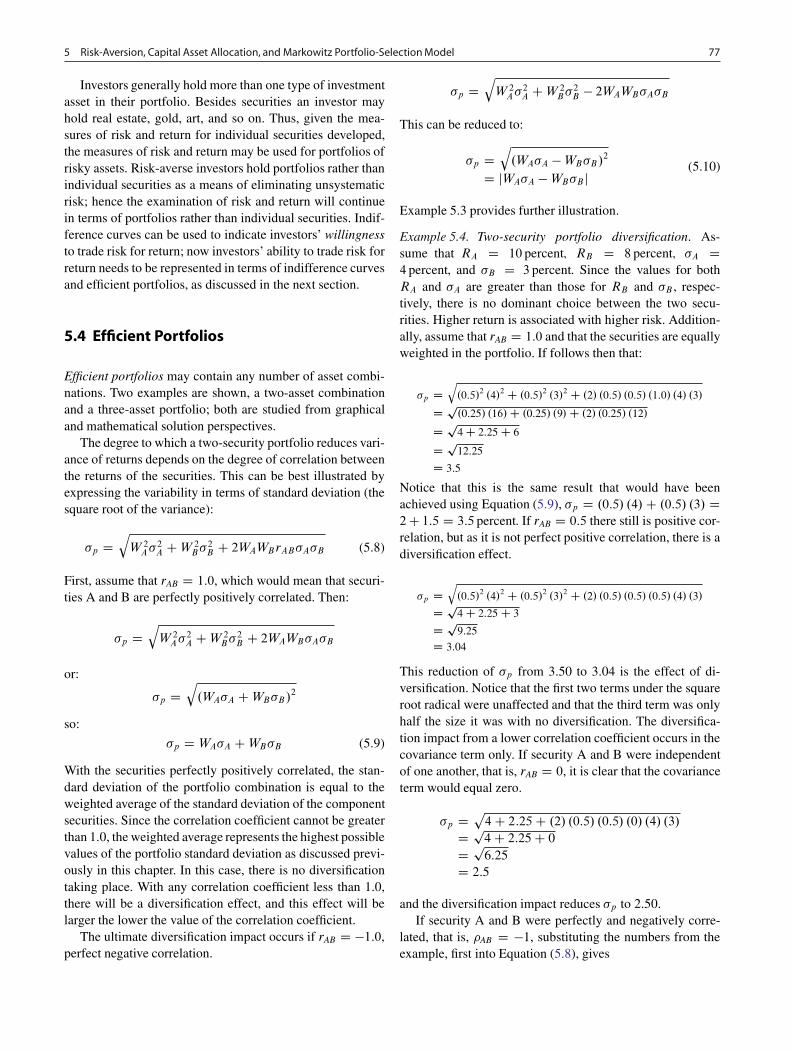
The degree to which a two-security portfolio reduces vari-ance of returns depends on the degree of correlation betweenthe returns of the securities. This can be best illustrated byexpressing the variability in terms of standard deviation (thesquare root of the variance):

�p DqW 2A�

2A CW 2

B�2B C 2WAWBrAB�A�B (5.8)

First, assume that rAB D 1:0, which would mean that securi-ties A and B are perfectly positively correlated. Then:

�p DqW 2A�

2A CW 2

B�2B C 2WAWB�A�B

or:

�p Dq.WA�A CWB�B/

2

so:

�p D WA�A CWB�B (5.9)

With the securities perfectly positively correlated, the stan-dard deviation of the portfolio combination is equal to theweighted average of the standard deviation of the componentsecurities. Since the correlation coefficient cannot be greaterthan 1.0, the weighted average represents the highest possiblevalues of the portfolio standard deviation as discussed previ-ously in this chapter. In this case, there is no diversificationtaking place. With any correlation coefficient less than 1.0,there will be a diversification effect, and this effect will belarger the lower the value of the correlation coefficient.

The ultimate diversification impact occurs if rAB D �1:0,perfect negative correlation.

�p DqW 2A�

2A CW 2

B�2B � 2WAWB�A�B

This can be reduced to:

�p Dq.WA�A �WB�B/

2

D jWA�A �WB�B j(5.10)

Example 5.3 provides further illustration.

Example 5.4. Two-security portfolio diversification. As-sume that RA D 10 percent; RB D 8 percent; �A D4 percent, and �B D 3 percent. Since the values for bothRA and �A are greater than those for RB and �B , respec-tively, there is no dominant choice between the two secu-rities. Higher return is associated with higher risk. Addition-ally, assume that rAB D 1:0 and that the securities are equallyweighted in the portfolio. If follows then that:

�p Dq.0:5/

2 .4/2 C .0:5/

2 .3/2 C .2/ .0:5/ .0:5/ .1:0/ .4/ .3/

D p.0:25/ .16/C .0:25/ .9/C .2/ .0:25/ .12/

D p4 C 2:25 C 6

D p12:25

D 3:5

Notice that this is the same result that would have beenachieved using Equation (5.9), �p D .0:5/ .4/C .0:5/ .3/ D2C 1:5 D 3:5 percent. If rAB D 0:5 there still is positive cor-relation, but as it is not perfect positive correlation, there is adiversification effect.

�p Dq.0:5/

2 .4/2 C .0:5/

2 .3/2 C .2/ .0:5/ .0:5/ .0:5/ .4/ .3/

D p4 C 2:25 C 3

D p9:25

D 3:04

This reduction of �p from 3.50 to 3.04 is the effect of di-versification. Notice that the first two terms under the squareroot radical were unaffected and that the third term was onlyhalf the size it was with no diversification. The diversifica-tion impact from a lower correlation coefficient occurs in thecovariance term only. If security A and B were independentof one another, that is, rAB D 0, it is clear that the covarianceterm would equal zero.

�p D p4C 2:25C .2/ .0:5/ .0:5/ .0/ .4/ .3/

D p4 C 2:25 C 0

D p6:25

D 2:5

and the diversification impact reduces �p to 2.50.If security A and B were perfectly and negatively corre-

lated, that is, �AB D �1, substituting the numbers from theexample, first into Equation (5.8), gives

78 C.-F. Lee et al.

�p D p4C 2:25C .2/ .0:5/ .0:5/ .�1:0/ .4/ .3/

D p6:25 � 6

D p0:25

D 0:5

and into Equation (5.10):

�p D .0:5/ .4/ � .0:5/ .3/ D 2 � 1:5 D 0:5

with the appropriate weighting factors, the �p may be re-duced to zero if there is negative correlation. For example,if WA D 3=7 and WB D 4=7 in this problem:

�p D .3=7/ .4/� .4=7/ .3/D 0

5.4.1 Portfolio Combinations

Assume that the actual correlation coefficient is 0.50. Byvarying the weights of the two securities and plotting thecombinations in the risk-return space, it is possible to derivea set of portfolios (see Table 5.3) that form an elliptical curve(see Fig. 5.6). The amount of curvature in the ellipse varieswith the degree of correlation between the two securities. Ifthere were perfect positive correlation, all of the combina-tions would lie on a straight line between points A and B.If the combination were plotted with the assumption of per-fect negative correlation, the curvature would be more pro-nounced and one of the points .WA D 0:43;WB D 0:57/

would actually be on the vertical axis (a risk of zero).This process could be repeated for all combination of in-

vestments; the result is graphed in Fig. 5.7. In Fig. 5.7 thearea within curve XVYZ is the feasible opportunity set rep-resenting all possible portfolio combinations. The curve YVrepresents all possible efficient portfolios and is the efficientfrontier. The line segment VX is on the feasible opportunityset, but not on the efficient frontier; all points on VX representinefficient portfolios.

The portfolios and securities that lie on the frontier VX inFig. 5.7 would not be likely candidates for investors to hold.This is so because they do not meet the criteria of maximizingexpected return for a given level of risk or minimizing risk

Table 5.3 Possible risk-return combination .RA D 0:10; RB D0:08; �A D 0:04; �B D 0:03; �AB D 0:5/

Portfolio WA WB RP (percent) �P (percent)

1 1:00 0:00 10:0 4:00

2 0:75 0:25 9:5 3:44

3 0:50 0:50 9:0 3:04

4 0:25 0:75 8:5 2:88

5 0:00 1:00 8:0 3:00

Fig. 5.6 The relationship between correlation and portfolio risk

Fig. 5.7 The minimum-variance set

for a given level of return. This is easily seen by comparingthe portfolio represented by points X and X 0. As investorsalways prefer more expected return than less for a given levelof risk, X 0 is always better than X . Using similar reasoning,investors would always prefer V to X because it has both ahigher return and a lower level of risk. In fact, the portfolioat point V is identified as the minimum-variance portfolio,because no other portfolio exists that has a lower variance.

For each of the combinations of individual securities andinefficient portfolios in Fig. 5.7 there is a corresponding port-folio along the efficient frontier that either has a higher returngiven the same risk or a lower risk given the same return.However, points on the efficient frontier do not dominateone another. While point Y has considerably higher returnthan point V , it also has considerably higher risk. The opti-

5 Risk-Aversion, Capital Asset Allocation, and Markowitz Portfolio-Selection Model 79

Fig. 5.8 Indifference curves and the minimum-variance set

mal portfolio along the efficient frontier is not unique withthis model and depends upon the risk/return tradeoff utilityfunction of each investor. Portfolio selection, then, is deter-mined by plotting investors’ utility functions together withthe efficient-frontier set of available investment opportuni-ties. No two investors will select the same portfolio except bychance or if their utility curves are identical. In Fig. 5.8, twosets of indifference curves labeled U and U 0 are shown to-gether with the efficient frontier. The U curves have a higherslope, indicating a greater level of risk aversion. The investoris indifferent to any combination of Rp and �p along a givencurve, for example, U1; U2, or U3. The U 0 curve would beappropriate for a less risk-averse investor – that is, one whowould be willing to accept relatively higher risk to obtainhigher levels of return. The optimal portfolio would be theone that provides the highest utility – a point in the north-west direction (higher return and lower risk). This point willbe at the tangent of a utility curve and the efficient frontier.The tangency point investor in Fig. 5.8 is point X 0; for therisk-averse it is point Y . Each investor is logically selectingthe optimal portfolio given his or her risk-return preference,and neither is more correct than the other.

Individual investors sometimes find it necessary to restricttheir portfolios to include a relatively small number of secu-rities. Mutual-fund portfolios, on the other hand, often con-tain securities from more than 500 different companies. Togive some idea of the number of securities that is necessaryto achieve a high level of diversification, Levy and Sarnat(1971) considered a naïve strategy of equally weighted port-folios – that is, of dividing the total investment into equalproportions among component securities. Plotting the vari-ance of the portfolios developed in this manner against the

number of securities making up the portfolios will result ina function similar to that illustrated in Fig. 5.9. As shown,the additional reduction in portfolio variance rapidly levelsoff as the number of securities is increased beyond five. Anearlier study by Evans and Archer (1968) shows that the per-centage of diversification that can be achieved with randomlyselected, equally weighted portfolios level off rapidly beyonda portfolio size of about 15.

5.4.2 Short Selling

Short selling (or “going short”) is a very regulated type ofmarket transaction. It involves selling shares of a stock thatare borrowed in expectation of a decline in the security’sprice. When and if the price declines, the investor buys anequivalent number of shares of the same stock at the newlower price and returns to the lender the stock that was bor-rowed. The Federal Reserve Board requires short selling cus-tomers to deposit 50% of the net proceeds of such short saleswith the brokerage firm carrying out the transaction. Anotherkey requirement of a short sale, set by the Securities and Ex-change Act of 1934, is that the short sale must occur at aprice higher than the preceding sale – or at the same price asthe preceding sale, if that took place at a higher price than apreceding price. This is the so-called uptick or zero-tick rule.It prevents the price of a security from successively fallingbecause of continued short selling.

Relaxing the assumption of no short selling in this de-velopment of the efficient frontier involves a modification ofthe analysis of the previous section. The efficient frontier an-alyzed in the previous sections was bounded on both endsby Y and the minimum variance portfolio V , respectively,as shown in Fig. 5.7. Point Y is called the maximum-returnportfolio, as there is no other portfolio with a higher return.This point is normally an efficient security or portfolio withthe greatest level of risk and return. It could also be a portfo-lio of securities, all having the same highest levels of risk andreturn. Point Z is normally a single security with the lowestlevel of return, although it could be a portfolio of securities,all having the same low level of return.

The Black (1972) model is identical to the Markowitzmodel except that it allows for short selling.5 That is, thenonnegativity constraint on the amount that can be investedin each security is relaxed,WA ? 0. A negative value for theweight invested in a security is allowed, tantamount to allow-ing a short sale of the security. The new efficient frontier thatcan be derived with short selling is shown in Fig. 5.10a.

5 Most texts do not identify the Markowitz model with restrictions onshort sale. Markowitz (1952), in fact, excluded short sales.

80 C.-F. Lee et al.

Fig. 5.9 Native diversificationreduces risk to the systematiclevel in a randomly selectedportfolio

The major difference between the frontier in Fig. 5.10a(short selling) and Fig. 5.10b (no short selling) is the disap-pearance of the end points Y and Z. An investor could sellthe lowest-return security .Y /. If the number of short sales isunrestricted, then by a continuous short selling ofX and rein-vesting in Y the investor could generate an infinite expectedreturn. Hence the upper bound of the highest-return portfoliowould no longer be Y but infinity (shown by the arrow on thetop of the efficient frontier). Likewise the investor could shortsell the highest-return security U and reinvest the proceedsinto the lowest-yield security X , thereby generating a returnless than the return on the lowest-return security. Given no re-striction on the amount of short selling, an infinitely negativereturn can be achieved, thereby removing the lower boundof X on the efficient frontier. But rational investors will notshort sell a high-return stock and buy a low-return stock andbuy a low-return stock.

The portfolios on VZ0 always dominate those of VX, asshown in Fig. 5.10a.

Whether an investor engages in any of this short-sellingactivity depends on the investor’s own unique set of indiffer-ence curves. Hence, short selling generally will increase therange of alternative investments from the minimum-varianceportfolio to plus or minus infinity. However, in the Blackmodel with short selling, no provision was made for theSEC margin requirement. Dyl (1975) imposed the marginrequirement on short selling and added it to the Markowitzdevelopment of the efficient frontier.

The Dyl model. Dyl introduced short selling with margin re-quirements by creating a new set of risky securities, the onessold short, which are negatively correlated with the exist-ing set of risky securities. These new securities greatly en-hance the diversification effect when they are placed in port-folios. The Dyl model affects the efficient frontier in twoways: (1) If the investor were to combine in equal weightany long position in a security or portfolio with a short posi-tion in a security or a portfolio, the resulting portfolio wouldyield zero return and zero variance and (2) any combina-tion of unequal weighted long or short positions would yield

Fig. 5.10 (a) The efficient frontier with short selling. (b) Efficient fron-tiers with and without short selling and margin requirements

portfolios with higher returns and lower risk levels. Overall,these two effects will yield an efficient frontier that domi-nates the Markowitz efficient frontier. Figure 5.10b comparesthe Dyl and Markowitz efficient frontiers.

5 Risk-Aversion, Capital Asset Allocation, and Markowitz Portfolio-Selection Model 81

Even though the inclusion of short selling changes thelocation and boundaries of the efficient frontier, the concav-ity of the curve is still intact. This is important in that it pre-serves the efficient frontier as the locus of optimal portfoliosfor risk-average investors. As long as the efficient frontierremains concave, by using indifference curves it will be pos-sible to locate the optimal portfolio for each investor.

Techniques for calculating the efficient frontier with shortselling. Since there are thousands of securities from whichthe investor can choose for portfolio formation, it can be verycostly and time consuming to calculate the efficient frontierset. One way of determining the optimal investment propor-tions in a portfolio is to hold the return constant and solvefor the weighting factors (W1 : : : ;Wn for n securities) thatminimize the variance, given the constraint that all weightssum to one and that the constant return equals the expectedreturn developed from the portfolio. The optimal weights canthen be obtained by minimizing the Lagrange function C forportfolio variance.

C DnPiD1

nPjD1

WiWj rij �i�j C �1

1�

nPiD1

Wi

C�2�E� �

nPiD1

WiE .Ri /

� (5.11)

in which �1 and �2 are the Lagrange multipliers, E� andE .Ri / are targeted rate of return and expected rate of returnfor security i , respectively, �ij is the correlation coefficientbetween Ri and Rj , and other variables are as previouslydefined.

Function C has nC 2 unknowns:W1; : : : ;Wn; �1, and �2.By differentiatingC with respect toWi; �1 and �2 and equat-ing the first derivatives to zero, nC2 equations can be derivedto solve for n C 2 unknowns. As shown in the empirical ex-ample later in this chapter, matrix algebra is best suited to thissolution process. By using this approach the minimum vari-ance can be computed for any given level of expected portfo-lio return (subject to the other constraint that the weights sumto one). In practice it is best to use a computer because of theexplosive increase in the number of calculations as the num-ber of securities considered grows. The efficient set that isgenerated by the aforementioned approach [Equation (5.11)]is sometimes called the minimum-variance set because of theminimizing nature of the Lagrangian solution.

Thus far no specific distribution for measuring returns hasbeen assumed. In most cases specific distribution of returnswill be needed when applying the portfolio model. The nor-mal and log normal are two of the most commonly useddistribution.

The normal distribution. As you undoubtedly are aware,the normal (probability) distribution is a bell-shaped curvecentered on the mean of a given population or sample distri-

bution. The area under the curve is an accumulation of prob-abilities that sum to one. With half of the area lying to theleft and half to the right of the mean, probability statementsmay be made about the underlying sample that makes up thedistribution.

Within the scope of the Markowitz model, the normaldistribution may be applied because of the use of the mean-variance assumptions. The formation of probability state-ments from the underlying sample is a result of the standarddeviation (square root of the variance) quantifying the spreadof the distribution. If the sample is normally distributed, ap-proximately 68% of the observations will lie within one stan-dard deviation on either side of the mean, approximately 95%will lie within two standard deviations, and approximately99% will lie within three standard deviations. This ability toascertain intervals of confidence for the observations allowsthe utilization of the normal distribution to predict rangeswithin which the portfolio returns will lie.

Utilizing the standard normal distribution (mean of zero,standard deviation of one), any set of mean-variance data canbe standardized to develop probability statements about re-turns on a given portfolio. Standardization is an algebraic op-eration in which the mean is subtracted from a given returnand this difference is divided by the standard deviation. Theresultant metric is then standard normal and can be comparedwith tabulated values to calculate probabilistic quantities ofoccurrence. Within this framework, any hypothesized levelof return can be assigned a probability of occurrence given aprobabilistic value of occurrence that is based upon the na-ture of the sample.

For expository purposes, suppose the mean return on aparticular investment is 10% for a given period, and that his-torically these returns have a variance of 0.16%. It is of in-terest to know what the probabilities are of obtaining a 15%or greater return, or a return less than or equal to 8%. Theseprobabilities may be evaluated by using the normal distribu-tion, as stated in notation below:

P�X 0:15

ˇ̌ˇRp D 0:1; �2p D 0:0016

P�X � 0:18

ˇ̌ˇRp D 0:1; �2p D 0:0016

by standardizing the probability statements to z values:

P

z 0:15� 0:1

0:04D 1:25

P

z � 0:08� 0:1

0:04D �0:5

(5.12)

These standardized values can then be compared with thetabulated z values found in tables of the standardized nor-mal distribution. For z 1:25 the probability is 10.56%

82 C.-F. Lee et al.

(50% – 39.44%), and for z D �0:05 the probability is0.3085. Therefore this investment has an 11.51% chance ofobtaining a 15% or more return, and a 30.85% chance of ob-taining 8% or less.

It is extremely difficult to make probabilistic statementswhen using the normal distribution. Given that the returndata utilized are ex post, the predictive ability of the nor-mal distribution based on historical data is limited. The pastdoes not always predict the future; hence, this problem issomewhat alleviated by an assumption that the security underconsideration is in a static state. Nevertheless, as shown byresearch and common sense, this assumption is rather bold,and the use of the normal distribution should be limited tocomparisons of various past portfolio returns.

Another difficulty with the normal distribution is that ifthe distribution of the sample is skewed in any way, the stan-dard deviation will not properly reflect the equivalent areasunder the curve on either side of the mean. This problem willbe discussed and solved in the next section through the appli-cation of the log normal distribution. A variable is log nor-mally distributed if a logarithm of this variable is normallydistributed.

The log normal distribution. The log normal distributiondiscussed in the next chapter will explore further of this sec-tion. The approach outlined in the last section for delineat-ing the efficient frontier assumes that the security-return dataare normally distributed. In reality, most financial researcherswould agree that security-return data tend to be positivelyskewed. This skewness can be a serious problem in accu-rately developing the efficient frontier with the Markowitzmodel because of the assumption that only the first two mo-ments of the return distribution, mean and variance, are im-portant.

One reason for returns being positively skewed is the in-ability of the investor to lose more than 100% of his or herinvestment, effectively creating a lower bound to portfolio re-turns. This is called the limited-liability constraint. But sincecapital gains and dividends could conceivably be infinite, theupper tail of the distribution of returns has no upper bounds.The range of probable returns is spread towards the positiveside and therefore contains a potential bias when it is utilizedin developing statistical estimates.

If the return distributions are significantly skewed, the ef-ficient frontier can be more accurately determined with theuse of logarithmically transformed holding-period returns.That is, each holding-period return for security i withholding period T .1 C RiT / is transformed by computing itsnatural logarithm, ln.1 C RiT/. The logarithmic transforma-tion converts a data set of discretely compounded returns intocontinuously compounded returns. The distribution of dis-crete time returns will be more positively skewed the largerthe differencing interval used to measure the returns; that is,

if skewness exists in the return distribution, annual data willbe more positively skewed than monthly data, which will bemore skewed than weekly data.

The continuous compounding implied in the logarith-mically transformed data will virtually eliminate any posi-tive skewness existing in the raw return data when rates ofreturn are log normally distributed. In practice, it is pos-sible to directly derive the efficient frontier using meansand variances of logarithmically transformed data. Underthis circumstance, assume that utility functions use contin-uous returns and variances, and then use the ln.1 C Rp/

transformation on discrete data. To deal with the untrans-formed log normally distributed data, Elton et al. (1976) usethe mean and variance of log normal distributed as definedin Equations (5.13) and (5.14) to derive the efficient frontier.In other words, they first delineate the efficient frontier byusing the means and variances of the untransformed data andthen use Equations (5.13) and (5.14) to determine the subsetof the ŒE.1 C Rp/; �.1 C Rp/ efficient frontier in terms oflog-transformed data, ln.1CRp/.

E.1CRp/ D eE.rp/C1=2�2 (5.13)

where rp D ln.1CRp/ and � is the standard deviation of rp .

�2.1CRp/ D�

e2E.rp/C�2 �

e�2 � 1

(5.14)

where rp D ln.1 C Rp/ and �2 D Var�rp�. Use of the log-

arithmic transformation can also be shown to eliminate lessdesirable portfolios in the lowest-return segment of the effi-cient frontier computer using the raw data.6 Before movingon to an example, however, it will be useful to briefly sum-marize the portfolio-selection process.

Again, the Markowitz model of portfolio selection is amathematical approach for deriving optimal portfolios; thatis, portfolios that satisfy the following conditions.

1. The least risk for a given level of expected return(minimum-variance portfolios).

2. The greatest expected return for a given level of risk (effi-cient portfolios).

How does a portfolio manager apply these techniques in thereal world?

The process would normally begin with a universe ofsecurities available to the fund manager. These securitieswould be determined by the goals and objectives of themutual fund. For example, a portfolio manager who runsa mutual fund specializing in health-care stocks would berequired to select securities from the universe of health-carestocks. This would greatly reduce the analysis of the fundmanager by limiting the number of securities available.

6 See Baumol (1963).

5 Risk-Aversion, Capital Asset Allocation, and Markowitz Portfolio-Selection Model 83

The next step in the process would be to determine theproportions of each security to be included in the portfo-lio. To do this, the fund manager would begin by setting atarget rate of return for the portfolio. After determining thetarget rate of return, the fund manager can determine the dif-ferent proportions of each security that will allow the portfo-lio to reach this target rate of return.

The final step in the process would be for the fund man-ager to find the portfolio with the lowest variance given thetarget rate of return. The next section uses a graphical ap-proach to derive the optimal portfolios for three securities.

5.4.3 Three-Security Empirical Solution

To facilitate a realistic example, actual data have been takenfrom a set of monthly returns generated by the Dow-Jones30 Industrials. This example focuses on the returns and riskof the first three industrial companies – AXP (AmericanExpress), XOM (Exxon Mobil), and JNJ (Johnson &Johnson) – for the period January 2001–September 2007.The data used are tabulated in Table 5.4. Both graphical andmathematical analyses are employed to obtain an empiricalsolution.

Graphical analysis. To begin to develop the efficient frontiergraphically, it is necessary to move from the three dimen-sions necessitated by the three-security portfolio to a two-dimensional problem by transforming the third security intoan implicit solution from the other two.7 To do this it mustbe noted that since the summation of the weights of the threesecurities is equal to unity, then implicitly:

W3 D 1 �W1 �W2 (5.15)

Additionally, the above relation may be substituted intoEquation (5.1):

E�Rp� D W1E .R1/CW2E .R2/CW3E .R3/

D W1E .R1/CW2E .R2/C .1 �W1 �W2/E .R3/

D W1E .R1/CW2E .R2/C E .R3/

�W1E .R3/�W2E .R3/ (5.16)

Table 5.4 Data for three securitiesCompany E .ri / �2i Cov

�Ri ; Rj

�

JNJ 0:0053 0:0455 �12 D 0:0009

AXP 0:0055 0:0614 �23 D 0:0010

XOM 0:0126 0:0525 �13 D 0:0004

7 The process of finding the efficient frontier graphically described inthis section was originally developed by Markowitz (1952). Francis andArcher (1979) have discussed this subject in detail.

D ŒE .R1/� E .R3/W1 C ŒE .R2/

�E .R3/W2 C E .R3/

Finally, inserting the values for the first and second securitiesyields:

E�Rp� D .0:0053� 0:0126/W1 C .0:0055� 0:0126/

W2 C 0:0126 (5.17)

D �0:0073W1 � 0:0071W2C0:0126

As can be seen, Equation (5.17) is a linear function in twovariables and as such is readily graphable. Since given a cer-tain level of portfolio return the function will solve jointly forthe weights of securities 1 and 2, it solves indirectly for theweight of security 3.

The variance formula shown in Equation (5.2) is con-verted in a similar manner by substituting in Equation (5.15)as follows:

�2p D3X

iD1

3X

jD1WiWjCov

�Ri;Rj

� D Var�Rp�

D W 21 �11 CW 2

2 �22 CW 23 �33 C 2W1W2�12

C2W1W3�13 C 2W2W3�23

D W 21 �11 CW 2

2 �22 C .1 �W1 �W2/2 �33�12

C2W1W2 C 2W1 .1 �W1 �W2/ �13

C2W2 .1 �W1 �W2/ �23

D .�11 C �33 � 2�13/W 21 C .2�33 C 2�12

�2�13 � 2�23/W1W2

C .�22 C �33 � 2�23/W22 C .�2�33 C 2�13/W1

C .�2�33 C 2�13/W2 C �33 (5.18)

Inserting the covariances and variances of the three securitiesfrom Table 5.4:

�2p D Œ0:0455C 0:0525� 2 .0:0004/W 21 C Œ2 .0:0525/

C2 .0:0009/ � 2 .0:0004/ � 2 .0:0010/W1W2

CŒ0:0614C 0:0525� 2 .0:0010/W 22

CŒ�2 .0:0525/C 2 .0:0004/W1

CŒ�2 .0:0525/C 2 .0:0010/W2 C 0:0525

D 0:0972W 21 C 0:104W1W2 C 0:1119W 2

2

�0:1042W1 � 0:103W2 C 0:0525 (5.19)

84 C.-F. Lee et al.

Minimum-risk portfolio. Part of the graphical solution is thedetermination of the minimum-risk portfolio. Standard par-tial derivatives are taken of Equation (5.18) with respect tothe directly solved weight factors as follows:

@�2p

@W1

D 2 .�11 C �33 � 2�13/W1 C .2�33 C 2�12

�2�13 � 2�23/W2 C .�2�33 C 2�13/ D 0

(5.20)@�2p

@W2

D .2�33 C 2�12 � 2�13 � 2�23/W1

C2 .�22 C �33 � 2�23/W2

C .2�23 � 2�33/ D 0

When these two partial derivatives are set equal to zero andthe unknown weight factors are solved for, the minimum riskportfolio is derived. Using the numeric values from Table 5.4:

@�2p

@W1

D 2Œ0:0455C 0:0525� 2 .0:0004/W1 C Œ2 .0:0525/

C2 .0:0009/ � 2 .0:0004/� 2 .0:0010/

W2 C Œ�2 .0:0525/C 2 .0:0004/

D 0:1944W1 C 0:104W2 � 0:1042 D 0

@�2p

@W2

D Œ2 .0:0525/C 2 .0:0009/� 2 .0:0004/ � 2 .0:0010/

W1 C 2Œ.0:0614/C 0:0525� 2 .0:0010/W2 C Œ2 .0:0010/ � 2 .0:0525/ (5.21)

D 0:104W1 C 0:2238W2 � 0:103 D 0

By solving these two equations simultaneously the weightsof the minimum-risk portfolio are derived. This variance rep-resents the lowest possible portfolio-variance level achiev-able, given variance and covariance data for these stocks.This can be represented by the point V of Fig. 5.8. Thissolution is an algebraic exercise that yields W1 D 0:3857

and W2 D 0:2810 and, therefore, through Equation (5.15),W3 D 0:3333.

The iso-expected return line. The variance and returnequations have been derived, and it is now time to com-plete the graphing procedure. To begin the graphing, the iso-expected return function lines must be delineated given var-ious levels of expected return. The iso-expected return lineis a line that has the same expected return on every pointof the line. Utilizing Equation (5.17), three arbitrary returnsare specified: 0.0082, 0.01008, 0.01134 (these correspondto 70, 80, and 90% annual returns of Exxon Mobil). Thesethree monthly returns are then set equal to Equation (5.17),and graphing is now possible by setting W1 equal to zero or

Table 5.5 Iso-return linesTarget return

0:0082 0:01008 0:01134

W2 W1 W1 W1

�1:0 1:5753 1:3178 1:1452

�0:5 1:0890 0:8315 0:6589

0:0 0:6027 0:3452 0:1726

0:5 0:1164 �0:1411 �0:31371:0 �0:3699 �0:6274 0:8000

other values to solve for W2. For example, if W2 D 0 andE�Rp� D 0:0082, then W1 can be solved as follows (see

Table 5.5 for final results).

0:0082 D �0:0073W1 � 0:0071 .0/C 0:0126

0:0073W1 D 0:0126� 0:0082 D 0:01154

W1 D 0:6027

In a similar fashion, other points are calculated and are listedin Table 5.5. A line may be drawn between the points to de-velop the various iso-expected return function lines.

There are a multitude of possible return functions, butonly these three lines .IR1; IR2 and IR3) in terms of the datalisted in Table 5.5 are shown in Fig. 5.11.

In Fig. 5.11 vertical axis and horizontal axis representW1

and W2, respectively.Each point on the iso-expected return line of Fig. 5.11 rep-

resents a different combination of weights placed in the threesecurities. The issue now is to determine the portfolio thatlies on the iso-expected return line with the lowest variance.Table 5.6 shows the portfolio variances as we move alongthe iso-expected return line. For example, moving along theiso-expected return line associated with an expected returnof 0.82%, note that the minimum variance portfolio is as-sociated with weights of 0.2577 in security 2 and 0.3521 insecurity 1.

Iso-variance ellipses. As shown in Table 5.6 the minimum-variance portfolio can be found by moving along the iso-expected return line until the minimum-variance portfolio isreached. To better visualize this, examine the variance ofa portfolio as the proportions in security 1 and security 2are changed. A plot of these points will allow the family ofiso-variance ellipses to be traced. The iso-variance ellipsesare the ellipses that have the same variance on every pointof this ellipse curve. It should be noted that an ellipse isan egg-shaped circle of points with a common center andorientation. The minimum-risk portfolio variance is the cen-ter of all possible ellipses as it has the least risk. It will bedesirable, then, to find this minimum risk value, as no otherweighting scheme of these three securities will develop alesser risk. The solutions of Equation (5.21) have determinedthat the weights associated with the minimum-risk portfolioare W1 D 0:3857; W2 D 0:2810, and W3 D 0:3333. Substi-

5 Risk-Aversion, Capital Asset Allocation, and Markowitz Portfolio-Selection Model 85

Fig. 5.11 Iso-return lines

Table 5.6 Portfolio variancealong the iso-return line

0.0082 0.01008 0.01134

w2 w1 Var w1 Var w1 Var

�1 1:5753 0.1806 1:3178 0.1618 1:1452 0.1564

�0:75 1:3322 0.1225 1:0747 0.1091 0:9021 0.1074

�0:5 1:0890 0.0771 0:8315 0.0693 0:6589 0.0713

�0:25 0:8459 0.0447 0:5884 0.0423 0:4158 0.0479

0 0:6027 0.0250 0:3452 0.0281 0:1726 0.0374

0:0795 0:5254 0.0214 0:2679 0.0263 0:0953 0.0368

0:151 0:4559 0.0194 0:1983 0.0258 0:0257 0.0373

0:25 0:3596 0.0182 0:1021 0.0268 �0:0705 0.0397

0:2577 0:3521 0.0182 0:0946 0.0269 �0:0780 0.0400

0:5 0:1164 0.0242 �0:1411 0.0383 �0:3137 0.0549

0:75 �0:1267 0.0431 �0:3842 0.0626 �0:5568 0.0829

1 �0:3699 0.0748 �0:6274 0.0998 �0:8000 0.1238

Note: Underlined variances indicate minimum variance portfolios

tuting this information listed in Table 5.4 into Equation (5.2),the variance of the minimum-risk portfolio is:

Var�Rp� D

nX

iD1

nX

jD1WiWjCov

�RiRj

�

D W 21 �11 CW 2

2 �22 CW 23 �33 C 2W1W2�12

C2W2W3�23 C 2W1W3�13

D .0:3857/2 .0:0455/C .0:2810/2

.0:0614/C .0:3333/2 .0:0525/

C2 .0:3857/ .0:2810/ .0:0009/C2.0:2810/.0:3333/.0:0010/C 2.0:3857/

.0:3333/.0:0004/

D 0:017934

Note that the variance of the minimum-risk portfolio can beused as a base for graphing the iso-variance ellipses. It can

be completed by taking Equation (5.18) and holding one ofthe weights, say W2 portfolio variance Var

�Rp�, constant.

Bring the Var�Rp�

to the right-hand side of the equation andnotice that the equation is of a quadratic form and can besolved using the quadratic formula:

W1 D �b ˙ pb2 � 4ac2a

(5.22)

where:

a D all coefficients of W 21 ;

b D all coefficients ofW1; andc D all coefficients that are not multiplied by W1, orW 21 : or

a D �11 C �33 C �13;b D .2�33 C 2�12 � 2�13 � 2�23/W2 � 2�33 C 2�13; andc D .�22 C �33 � 2�23/W 2

2 C .�2�33 C 2�23/W2 C �33� Var

�Rp�.

86 C.-F. Lee et al.

Substituting the numbers from the data of Table 5.4 intoEquation (5.18) yields:

Var.Rp/ D 0:0972W21 C 0:104W1W2 C 0:1119W 2

2

�0:1042W1 � 0:103W2 C 0:0525

0 D 0:0972W21 C 0:104W1W2 C 0:1119W 2

2

�0:1042W1 � 0:103W2 C 0:0525�Var.Rp/

where:

a D 0:0972Ib D 0:104W2 � 0:1042I andc D 0:1119W 2

2 � 0:103W2 C 0:0525� Var.Rp/:

When these expressions are plugged into the quadraticformula:

W1 D � .0:104W2 � 0:1042/˙ pb2 � 4ac

2 .0:0972/(5.23)

where

b2 D .0:104W2 � 0:1042/2

4ac D 4f.0:0972/Œ0:1119W 22 � 0:103W2

C0:0525� Var.Rp/g

This is a solution for the two points of W1(W11 and W12)for a given portfolio variance and weight of the second se-curity .W2/. When selecting the level of Var .Rp/ it is bestto choose a value that is slightly larger than the minimum-risk value. This assures the calculation of a possible portfo-lio, since no portfolio of these three securities may have lessrisk. Additionally, an initial selection of a value for W2 closeto the minimum-risk portfolioW2 will be desirable.

In sum, Equation (5.23) can be used to construct the iso-variance ellipse for given Var .Rp/ in terms of arbitrary W2.By jointly considering iso-expected return lines and iso-variance ellipses, efficient portfolios can be identified that aredefined as the portfolios with the minimum variance giventhe expected rate of return. This task can be done by com-puter, as mentioned in the last section. To obtain the weightsof an efficient portfolio, the following set of instructions mustbe entered into the computer.

1. Find the portfolio weights that minimize portfoliovariance, subject to the target expected rate-of-returnconstraint. For this case, target rates of return are 0.82,1.008, or 1.1134%. The sum of the portfolio weights forall stocks in the portfolio must be equal to one. Mathemat-ically, this instruction is defined in Equation (5.15).

2. The expected return and variance for a three-security port-folio is defined in Equations (5.16) and (5.18), respec-tively.

3. The estimated expected return, variance, and covarianceas defined in Table 5.4 should be entered into the com-puter for estimation.

Using E.Rp/ D 0:82 percent as an example, W1 D 0 andW2 D 0:6197. From the relationship W3 D 1 � W1 �W2 D1 � 0 � 0:6197 D 0:3803. In other words, the point H rep-resents three portfolio weights for the three stocks. The com-puter substitutes weights, variances, and covariances (listedin Table 5.4) into Equation (5.18) to obtain portfolio vari-ance. The portfolio variance consistent with the weights ofpointH is computed. The computer now moves by some pre-determined distance either northeast or southwest along the0.82% iso-expected return line. From this kind of search, theminimum variance associated with this 0.82% iso-expectedreturn line is identified to be 0.0182, as indicated in Table 5.6.By a similar procedure, the minimum variances associatedwith 1.008 and 1.134% iso-expected return lines are identi-fied to be 0.0258 and 0.0368, respectively. When minimumvariances associated with predefined iso-expected return areidentified, the optimal weights associated with expected re-turns equal to 1.008 and 1.134% in terms of data indicated inTable 5.4 are also calculated. These results are indicated inTable 5.6.

Using the minimum variances associated with iso-expected returns (0.82, 1.008, and 1.134%), three iso-variance ellipses can be drawn as IV1; IV2, and IV3.

When Var.Rp/ D 0:0182 and W2 D 0:3, the quadraticformula from Equation (5.23) above yields two roots.

W11 D �.0:0730/Cp.0:0730/2�.�0:0052/

2.0:0972/

D 0:4247

W12 D �.0:0730/�p.0:0730/2�.�0:0052/2.0:0972/

D 0:3263

To solve for W11 and W12 we need b2 > 4ac. Solving for thevariance:

.0:104W2 � 0:1042/2 � 4f.0:0972/ > Œ0:1119W 22

�0:103W2 C 0:0525� Var.Rp/g

If W2 and Var .Rp/ are not selected so that b2 > 4ac,Equation (5.23) will require taking the square root of anegative number, and mathematically the solution will bean imaginary number. Solving W2 in terms of an imaginarynumber is not meaningful; therefore we only consider thecase when b2 > 4ac.

5 Risk-Aversion, Capital Asset Allocation, and Markowitz Portfolio-Selection Model 87

The variance chosen was the minimum variance of theportfolio associated with E.Rp/ D 0:0082. Actually, anyvariance might have realistically been chosen as long asit exceeded the minimum-risk portfolio variance. Table 5.7lists various W11 and W12 values for given levels of W2 andVar .Rp/. In addition, Table 5.7 presents the value of b2 and4ac to check whether or not the root is a real number. Itshould be noted that all possible variances are higher thanthe minimum-risk portfolio variance. Data from Table 5.7are used to draw three iso-variance ellipses, as indicated inFigs. 5.12 and 5.13.

The critical line and efficient frontier. After the iso-expectedreturn functions and iso-variance ellipses have been plot-ted, it is an easy task to delineate the efficient frontier. Bydefinition, the efficient portfolio is the portfolio with thehighest return for any given risk. In Fig. 5.13, the efficientportfolios are those where a given iso-expected return line isjust tangent to the variance ellipse. MRPABC is denoted as

the critical line; all portfolios that lie between points MRPand C are said to be efficient, and the weights of these port-folios may be read directly from the graph. From the graph,portfolio weights for the portfolios that minimize variances,given a 0.82, 1.008, or 1.134% expected rate of return arelisted in Table 5.6. It is possible, given these various weights,to calculate the E.Rp/ and the variances of these portfolios,as indicated in Table 5.8. The efficient frontier is then devel-oped by plotting each risk-return combination, as shown inFig. 5.14.

In this section a step-wise graphical approach has beenemployed to obtain optimal weights for a three-securityportfolio. In the next section a mathematical optimizationapproach is used to calculate the optimal weight for a three-security portfolio.

Mathematical analysis. The same efficient frontier can beobtained mathematically through the use of the Lagrangianmultipliers. The Lagrangian method allows the minimization

Table 5.7 Various W1 given W2 and Var.Rp/

W2 Var.Rp/ b b2 C 4 ac W11 W12

0:28 0:0182 �0:0751 0:0056 0:0142 0:0055 0:4385 0:3339

0:29 0:0182 �0:0740 0:0055 0:0138 0:0054 0:4325 0:3293

0:30 0:0182 �0:0730 0:0053 0:0135 0:0052 0:4247 0:3263

0:31 0:0182 �0:0720 0:0052 0:0131 0:0051 0:4149 0:3254

0:32 0:0182 �0:0709 0:0050 0:0128 0:0050 0:4025 0:3272

0:28 0:0258 �0:0751 0:0056 0:0066 0:0026 0:6707 0:1017

0:29 0:0258 �0:0740 0:0055 0:0062 0:0024 0:6652 0:0965

0:30 0:0258 �0:0730 0:0053 0:0059 0:0023 0:6594 0:0916

0:31 0:0258 �0:0720 0:0052 0:0055 0:0021 0:6534 0:0870

0:32 0:0258 �0:0709 0:0050 0:0052 0:0020 0:6470 0:0827

0:28 0:0368 �0:0751 0:0056 �0:0044 �0:0017 0:8268 �0:05430:29 0:0368 �0:0740 0:0055 �0:0048 �0:0019 0:8213 �0:05960:30 0:0368 �0:0730 0:0053 �0:0051 �0:0020 0:8157 �0:06470:31 0:0368 �0:0720 0:0052 �0:0055 �0:0021 0:8099 �0:06960:32 0:0368 �0:0709 0:0050 �0:0058 �0:0023 0:8039 �0:0742

Fig. 5.12 Iso-variance ellipses

88 C.-F. Lee et al.

Fig. 5.13 Iso-variance ellipsesand iso-return lines

Table 5.8 Weights, Rp , and �p for efficient points

Portfolio W1 W2 W3 E.Rp/ Var.Rp/ �.Rp/

A 0:3521 0:2577 0:3902 0:0082 0:0182 0:1349

B 0:1983 0:1510 0:0795 0:01008 0:0258 0:1606

C 0:3902 0:6507 0:8252 0:01134 0:0368 0:1918

Portfolios A, B, and C represent expected returns of 0.82, 1.008, and 1.134%, respectively

Fig. 5.14 The efficient frontierfor the data of Table 5.8

or maximization of an objective function when the objectivefunction is subject to some constraints.

One of the goals of portfolio analysis is minimizing therisk or variance of the portfolio, subject to the portfolioattaining some target expected rate of return, and also sub-ject to the portfolio weights’ summing to one. The problemcan be stated mathematically:

Min �2p DnX

iD1

nX

jD1WiWj�ij

Subject to

(a)nPiD1

WiE.Ri / D E�

where E� is the target expected return and

(b)nPiD1

Wi D 1:0

5 Risk-Aversion, Capital Asset Allocation, and Markowitz Portfolio-Selection Model 89

The first constraint simply says that the expected returnon the portfolio should equal the target return determinedby the portfolio manager. The second constraint says that theweights of the securities invested in the portfolio must sumto one.

The Lagrangian objective function can be written:

C DnX

iD1

nX

jD1WiWjCov

�RiRj

�C �1

1 �

nX

iD1Wi

!

C�2"E� �

nX

iD1WiE .Ri /

#(5.11)

Taking the partial derivatives of this equation with respectto each of the variables, W1;W2;W3; �1; �2 and setting theresulting five equations equal to zero yields the minimiza-tion of risk subject to the Lagrangian constraints. This sys-tem of five equations and five unknowns can be solved by theuse of matrix algebra. Briefly, the Jacobian matrix of theseequations is

2

66664

2�11 2�12 2�13 �1 �E .R1/2�21 2�22 2�23 �1 �E .R2/2�31 2�32 2�33 �1 �E .R3/1 1 1 0 0

E .R1/ E .R2/ E .R3/ 0 0

3

77775

2

66664

W1

W2

W3

�1�2

3

77775D

2

66664

0

0

0

1

E�

3

77775

(5.24)

Therefore, it is possible to premultiply both sides of thematrix Equation (5.24), AW D K, by the inverse of A (de-noted A�1) and solve for the W column. This is possiblebecause all values in the A and K matrices are known orarbitrarily set.

The first problem is the inversion of the matrix of coeffi-cients. First, derive the determinant of matrix A. Next, afterdeveloping the signed, inverted matrix of cofactors for A, di-vide the cofactors by the determinant, resulting in the inver-sion of the original matrix. Finally, premultiply the columnvector for the investment weights.

Plugging the data listed in Table 5.4 and E� D 0:00106

into the matrix above yields

2

666664

0:0910 0:0018 0:0008 �1 �0:00530:0036 0:1228 0:0020 �1 �0:00550:0008 0:0020 0:1050 �1 �0:01261 1 1 0 0

0:0053 0:0055 0:0126 0 0

3

777775

2

666664

W1

W2

W3

�1

�2

3

777775D

2

666664

0

0

0

1

0:00106

3

777775

(5.25)

When matrix A is properly inverted and postmultiplied by K,the solution vector A�1K is derived:

W A�1K266664

W1

W2

W3

�1�2

377775

D

266664

0:9442

0:6546

�0:59880:1937

�20:1953

377775

(5.26)

Using the matrix operation on the other two arbitrary returnsyields the results shown in Table 5.8.

As shown in the composition of Portfolios A, B, and C,the weights of security 3 are negative, implying that thissecurity should be sold short in order to generate an efficientportfolio. It should be noted that the results of Table 5.8 aresimilar to those of Table 5.6. Therefore, both graphical andmathematical methods can be used to calculate the optimalweights.

With the knowledge of the efficient-portfolio weights,given that E.Rp/ is equal to 0.00106, 0.00212, and 0.00318,the variances of the efficient portfolios may be derived fromplugging the numbers into Equation (5.2). Taking the squareroot of the variances to derive the standard deviation, the var-ious risk-return combinations can be plotted and the efficientfrontier graphed, as shown in Fig. 5.13 in the previous sec-tion. As can be seen from comparing this figure to the graphi-cal derivation of the efficient frontier derived graphically, theresults are almost the same.

5.4.4 Portfolio Determination with SpecificAdjustment for Short Selling

By using a definition of short sales developed by Lintner(1965) the computation procedure for the efficient frontiercan be modified. Lintner defines short selling as putting up anamount of money equal to the value of the security sold short.Thus the short sale is a use rather than a source of funds to theshort seller. The total funds the investor invests short, plus thefunds invested long, must add up to the original investment.The proportion of funds invested short is jXi j, since Xi < 0.The constraint in the minimization problem concerning theweights of the individual securities needs to be modified toincorporate this fact. Additionally, the final portfolio weight(output of the matrix inversion) must be rescaled so the sumof the absolute value of the weights equals one. By definingshort sales in this manner, the efficient frontier does not ex-tend to infinity (as shown in Fig. 5.10a) but resembles theefficient frontier in Fig. 5.10b.

Monthly rates of return for Johnson & Johnson, Amer-ican Express, and Exxon Mobile are used to perform theanalysis in this section. The sample period is from January

90 C.-F. Lee et al.

2001 to September 2007. The Markowitz model determinesoptimal asset allocation by minimizing portfolio variance us-ing a constrained optimization procedure:

Min Var�Rp� D

3X

iD1

3X

jD1WiWj�ij (5.2)

Subject to:

(a)3PiD1

WiE .Ri / D E� (5.1)

(b)3PiD1

jWi j D 1:0 (5.1)

Where the E� is the investors’ desired rate of return, andwhere the absolute value of the weights jWi j allows for agivenW to be negative (sold short) but maintains the require-ment that all funds are invested or their sum equals one.

The Lagrangian function is

Min L DnX

iD1

nX

jD1WiWj C �1

nX

iD1

�WiE .Ri /� E��

C�2

nX

iD1Wi � 1

!

Again, derivatives with respect to Wi ’s and �’s are found.Setting these equations equal to zero leaves the followingsystem of equations in matrix form:

C X K2

666666664

2�11 2�12 � � � 2�1n E .R1/ 1

2�21 2�22 � � � 2�2n E .R2/ 1

::::::

::::::

:::

2�n1 2�n2 � � � 2�nn E .Rn/ 1

E .R1/ E .R2/ � � � E .Rn/ 0 0

1 1 � � � 1 0 0

3

777777775

2

666666664

W1

W2:::

Wn

�1

�2

3

777777775

D

2

666666664

0

0

:::

0

E�1

3

777777775

To solve this matrix:

CX D KC�1CX D C�1K

IX D C�1KX D C�1K

where

C�1 is the inverse of matrix C andI is the identity matrix.

The solution to the above formula will give the weights interms of E�.

By using Johnson & Johnson, American Express, andExxon Mobile a three-security portfolio will be formed andoptimal weights will be solved for.

SecurityMonthlyE.Ri / �2i �12 �13 �23

JNJ 0.0053 0.0455 0.0009 0.0004 0.0010AXP 0.0055 0.0614XOM 0.0126 0.0525

Substituting these values into the matrix:2

666664

0:0910 0:0018 0:0008 0:0053 1

0:0018 0:0614 0:0020 0:0055 1

0:0008 0:0020 0:0525 0:0126 1

0:0053 0:0055 0:0126 0 0

1 1 1 0 0

3

777775

2

666664

W1

W2

W3

�1

�2

3

777775D

2

666664

0

0

0

E�1

3

777775

E� D 0:013

By solving using the identity-matrix technique the weightsfor the three securities can be obtained:

Johnson & Johnson D �0:0406American Express D �0:0146

Exxon Mobile D 1:0552

By using the following relationship to rescale these weightsso that the second constraint for the sum of the absolute val-ues of the weights to equal one is satisfied:

WjAj D jAjjAj C jBj C jC j (5.27)

The resealed absolute weights are:

WJNJ D 0:0406

0:0406C 0:0146C 1:0552D 0:0366

WAXP D 0:0146

0:0406C 0:0146C 1:0552D 0:0131

WXOM D 1:0552

0:0406C 0:0146C 1:0552D 0:9503

The return on this portfolio is:

Rp D .0:0366/ .0:0053/C .0:0131/ .0:0055/C .0:9503/

.0:0126/

D 1:22%

The variance:

�2p D .0:0366/2 .0:0455/C .0:0131/2 .0:0614/C .0:9503/2

.0:0525/C 2 .0:0366/ .0:0131/ .0:0009/C 2 .0:0366/

.0:9503/ .0:0004/C 2 .0:0131/ .0:9503/ .0:0010/

D 0:0475

5 Risk-Aversion, Capital Asset Allocation, and Markowitz Portfolio-Selection Model 91

5.4.5 Portfolio Determination Without ShortSelling

The minimization problem under study can be modified toinclude the restriction of no short selling by adding a thirdconstraint:

Wi 0; i D 1; : : : ; N

The addition of this nonnegativity constraint precludes neg-ative values for the weights (that is, no short selling). Theproblem now is a quadratic programming problem similar tothe ones solved so far, except that the optimal portfolio mayfall in an unfeasible region. In this circumstance the next bestoptimal portfolio is elected that meets all of the constraints.An example of this situation is shown in Fig. 5.15.8

In Fig. 5.15a the optimal portfolio is located in the regionof positive values for weights W �

i , and thereby satisfies the

Fig. 5.15 Optimal portfolio in feasible and unfeasible regions

8 In Fig. 5.15a and b the vertical axis is defined as .Rp � Rf /ı�p ,

which is the Sharpe performance measure as defined in Chap. 4..Rp � Rf /

ı�p is the objective function for portfolio optimization; it

will be explored in Chap. 8.

constraintW �i 0. In Fig. 5.15b the optimal portfolio shown

by W �i falls in a region where W1 are negative, and so the

constraint is not satisfied. The next best optimal portfolio isshown byB , and this is the solution of the problem that satis-fies the nonnegativity constraint. Additional discussion of theproblems is presented in later chapters. Most recently, Lewis(1988) has developed a simple algorithm for the portfolio-selection problem. His method is based on an interactive useof the Markowitz critical-line method for solving quadraticprograms. In Fig. 5.15a, b the vertical axis is defined as. NRp � Rf /

ı�p , this is a Sharpe performance mean, as de-

fined in Chap. 4, and can be regarded as the objective func-tion for a portfolio selection.

5.5 Conclusion

This chapter has focused on the foundations of Markowitz’smodel and on derivation of efficient frontier through the cre-ation of efficient portfolios of varying risk and return. It hasbeen shown that an investor can increase expected utilitythrough portfolio diversification as long as there is no perfectpositive correlation among the component securities. The ex-tent of the benefit increases as the correlation is lower, andalso increases with the number of securities included.

The Markowitz model can be applied to develop the effi-cient frontier that delineates the optimal portfolios that matchthe greatest return with a given amount of risk. Also, thisfrontier shows the dominant portfolios as having the lowestrisk given a stated return. This chapter has included meth-ods of solving for the efficient frontier both graphically andthrough a combination of calculus and matrix algebra, withand without explicitly incorporating short selling.

The next chapter will illustrate how the crushing compu-tational load involved in implementing the Markowitz modelcan be alleviated through the use of the index portfolio,and how the tenets of the Markowitz efficient frontier arestill met.

References

Alexander, G. J. and J. C. Francis. 1986. Portfolio analysis, Prentice-Hall, Englewood Cliffs, NJ.

Baumol, W. J. 1963. “An expected gain-confidence limit criterion forportfolio selection.” Management Science 10, 171–182.

Bertsekas, D. 1974. “Necessary and sufficient conditions for exis-tence of an optimal portfolio.” Journal of Economic Theory 8,235–247.

Black, F. 1972. “Capital market equilibrium with restricted borrowing.”Journal of Business 45, 444–455.

Blume, M. 1970. “Portfolio theory: a step toward its practicalapplication.” Journal of Business 43, 152–173.

92 C.-F. Lee et al.

Bodie, Z., A. Kane, and A. Marcus. 2006. Investments, 7th Edition,McGraw-Hill, New York.

Brealey, R. A. and S. D. Hodges. 1975. “Playing with portfolios.”Journal of Finance 30, 125–134.

Breen, W. and R. Jackson. 1971. “An efficient algorithm for solvinglarge-scale portfolio problems.” Journal of Financial and Quantita-tive Analysis 6, 627–637.

Brennan, M. J. 1975. “The optimal number of securities in a risky assetportfolio where there are fixed costs of transaction: theory and someempirical results.” Journal of Financial and Quantitative Analysis10, 483–496.

Cohen, K. and J. Pogue. 1967. “An empirical evaluation of alternativeportfolio-selection models.” Journal of Business 46, 166–193.

Dyl, E. A. 1975. “Negative betas: the attractions of selling short.”Journal of Portfolio Management 1, 74–76.

Elton, E. J. and M. Gruber. 1974. “Portfolio theory when invest-ment relatives are log normally distributed.” Journal of Finance 29,1265–1273.

Elton, E. J. and M. Gruber. 1978. “Simple criteria for optimal portfolioselection: tracing out the efficient frontier.” Journal of Finance 13,296–302.

Elton, E. J., M. Gruber, and M. E. Padberg. 1976. “Simple criteria foroptimal portfolio selection.” Journal of Finance 11, 1341–1357.

Elton, E. J., M. J. Gruber, S. J. Brown, and W. N. Goetzmann.2006. Modern portfolio theory and investment analysis, 7th Edition,Wiley, New York.

Evans, J. and S. Archer. 1968. “Diversification and the reduc-tion of dispersion: an empirical analysis.” Journal of Finance 3,761–767.

Fama, E. F. 1970. “Efficient capital markets: a review of theory andempirical work.” Journal of Finance 25, 383–417.

Feller, W. 1968. An introduction to probability theory and its applica-tion, Vol. 1, Wiley, New York.

Francis, J. C. and S. H. Archer. 1979. Portfolio analysis, Prentice-Hall,Englewood Cliffs, NJ.

Gressis, N., G. Philiippatos, and J. Hayya. 1976. “Multiperiod portfolioanalysis and the inefficiencies of the market portfolio.” Journal ofFinance 31, 1115–1126.

Henderson, J. and R. Quandt. 1980. Microeconomic theory: a mathe-matical approach, 3d Edition, McGraw-Hill, New York.

Lee, C. F. and A. C. Lee 2006. Encyclopedia of finance, Springer,New York.

Lee, C. F., J. C. Lee, and A. C. Lee. 2000. Statistics for business andfinancial economics, World Scientific Publishing Co, Singapore.

Levy, H. and M. Sarnat. 1971. “A note on portfolio selection andinvestors’ wealth.” Journal of Financial and Quantitative Analysis6, 639–642.

Lewis, A. L. 1988. “A simple algorithm for the portfolio selection prob-lem.” Journal of Finance 43, 71–82.

Lintner, J. 1965. “The valuation of risk assets and the selection ofrisky investments in stock portfolio and capital budgets.” Review ofEconomics and Statistics 47, 13–27.

Mao, J. C. F. 1969. Quantitative analysis of financial decisions,Macmillan, New York.

Maginn, J. L., D. L. Tuttle, J. E. Pinto, and D. W. McLeavey. 2007.Managing investment portfolios: a dynamic process, CFA InstituteInvestment Series, 3rd ed., Wiley, New Jersey.

Markowitz, H. M. 1952. “Portfolio selection.” Journal of Finance 1,77–91.

Markowitz, H. M. 1959. Portfolio selection. Cowles FoundationMonograph 16, Wiley, New York.

Markowitz, H. M.1976. “Markowitz revisited.” Financial AnalystsJournal 32, 47–52.

Markowitz, H. M. 1987. Mean-variance analysis in portfolio choice andcapital markets. Blackwell, Oxford.

Martin, A. D., Jr. 1955. “Mathematical programming of portfolio selec-tions.” Management Science 1, 152–166.

Merton, R. 1972. “An analytical derivation of efficient portfo-lio frontier.” Journal of Financial and Quantitative Analysis 7,1851–1872.

Mossin, J. 1968. “Optimal multiperiod portfolio policies.” Journal ofBusiness 41, 215–229.

Ross, S. A. 1970. “On the general validity of the mean-variance ap-proach in large markets,” in Financial economics: essays in honorof Paul Cootner, W. F. Sharpe and C. M. Cootner (Eds.). PrenticeHall, Englewood Cliffs, NJ, pp. 52–84.

Sharpe, W. F. 1970. Portfolio theory and capital markets, McGraw-Hill,New York.

Von Neumann, J. and O. Morgenstern. 1947. Theory of gamesand economic behavior, 2nd Edition, Princeton University Press,Princeton, NJ.

Wackerly, D., W. Mendenhall, and R. L. Scheaffer. 2007. Mathematicalstatistics with applications, 7th Edition, Duxbury Press, California.