CHAPTER NINE

THE DENSITY OF STATES AND ENTROPY

Introduction

In this chapter we will look again at the internal energy of a system and ask about the number of states

available to this system. In particular, we will examine the of the system, i.e., the numberdensity of states, , =ÐIÑof states available to a system within a given energy range between and . We will find that the densityI I � I$of states varies rapidly as the energy of the system changes. This discussion will lead naturally to the concept of

entropy, the tendancy of a system to move toward a state where there are a larger number of states available, i.e.,

toward a system.less ordered

Density of States

Consider the phase space diagram for a single free particle moving in one dimension within a fixed region

! � B � P I. If the particle has an energy , the momentum of the particle is given by

: œ „ #7IBÈ (9.1)

since the total energy of a free particle is just the kinetic energy. The number of “cells” in phase space which

represent all possible systems with energy is just the area of the phase space diagramless than I Ð œ : Î#7 ÑB#

depicted below divided by the size of a “cell” . We will denote the number of cells with energyÐ 2 œ : ; Ñ9 B B$ $less than by .I ÐIÑF

p

q

+p

-p

o

o 0 L

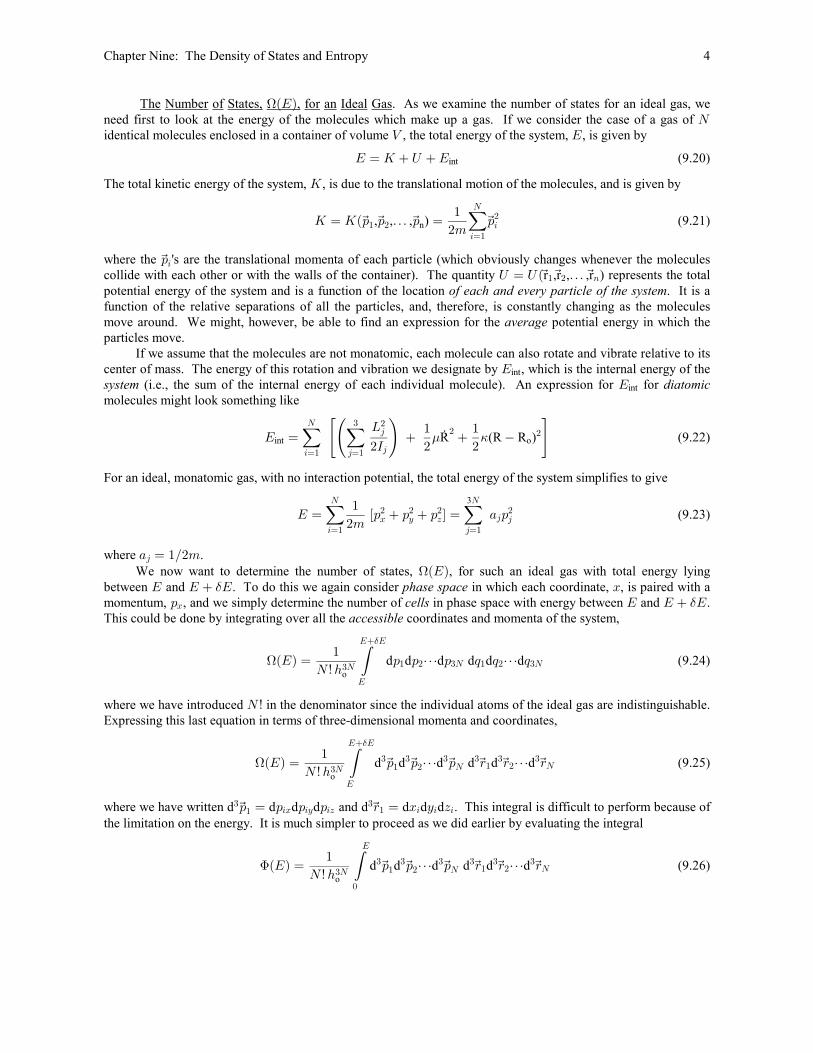
Figure 9.1 The region of phase space for a one-dimensional free particle bounded by the energy I œ :#7

#

and the dimensions .! � B � P

The number of cells in phase space (the number of microstates of the system) which correspond to a one-

dimensional, free particle with an energy between and , , must therefore be given byI I � I ÐIÑ$ H

H F $ F $F

ÐIÑ œ ÐI � IÑ � ÐIÑ œ I` ÐIÑ

`I (9.2)

or

H = $ÐIÑ œ ÐIÑ I (9.3)

where is the . In this particular example, we have=ÐIÑ density of states

F αÐIÑ œ œ #7I œ I#: P #P

2 2B B

9 9

È "# (9.4)

where is a constant given by . So we see that the number of states accessible to a single, one-α α œ )7P Î2È # #9

dimentional particle with energy between zero and is proportional to . But this is for a single, one-I I"#

dimensional particle. In three dimensions, we can also count the number of states (phase space cells) with energy

less than , but phase space in this case is three-dimensional, and we must consider the I six-dimensional volume

of phase space accessible to the single particle. If we assume the particle is confined to a cubic box, each

Chapter Nine: The Density of States and Entropy 2

dimension is equivalent, and we have

FÐIÑ º I"# (9.5)

for of the three conjugate pairs: ; ; and . This means that the number of cells with energy lesseach Bß : Cß : Dß :B C D

than for a free particle in three dimensions is given byI

FÐIÑ º I$# (9.6)

If we now ask about the number of states which are accessible to free particles moving in a three-dimensionalRcubic box, we would have

FÐIÑ º I$R# (9.7)

or

FÐIÑ œ )7P Î2 I œ )7Î2 Z IŠ ‹ Š ‹É É# # #9 9

$R $RR$R $R

# # (9.8)

provided that each of the particles is distinguishable. If the particles are not distinguishable, then we can

enterchange particles without actually changing the microstate of the system. The number of different ways we

can interchange N particles is N!, so that we have actually overcounted the number of microstates for this system.

Thus, for indistinguishable particles, the actual number of states with energy less than E is given by

(9.9)FÐIÑ œ )7Î2 IZ

Rx

R

9#

$RŠ ‹É $R#

We have demonstrated that the number of cells (or microstates) in phase space is proportional to the total energy

of the system raised to some power, which we can express in terms of the number of for thedegrees of freedom

system. In the case of three-dimensional particles free to move in a cubic box, there are degrees ofR œ $RÁfreedom We can therefore writeÞ

FÐIÑ œ )7Î2 IZ

Rx

R

9#Š ‹É Á

Á# (9.10)

To find the density of states we take the derivative of with respect to , and obtain= FÐIÑ ÐIÑ I

H $ = $ $F Á

ÐIÑ œ I œ ÐIÑ I œ )7Î2 I I` ÐIÑ Z

`I Rx # (9.11)

R

9# �"Š ‹É Á ˆ ‰Á

#

Now since the number of degrees of freedom is proportional to the number of particles in the system, weRtypically set , so that we haveˆ ‰Á Á

# #� " ¸

=ÐIÑ º I ÁÎ# (9.12)

The Density of States for Various Systems

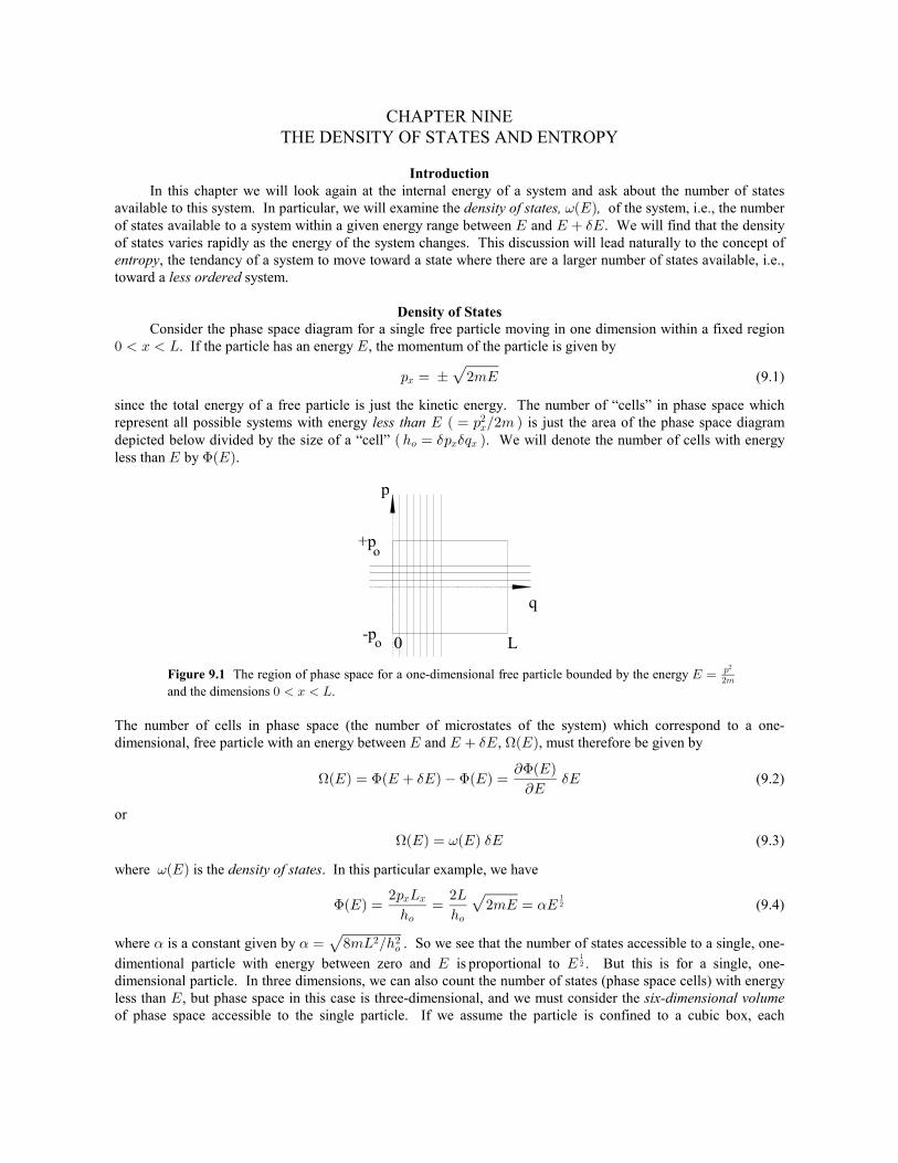
The energy for a one-dimensional simple harmonicThree-dimensional Simple Harmonic Oscillator.

oscillator is given by

I œ � 5B: "

#7 #

## (9.13)

so that the phase space diagram for such a system is an ellipse whose semi-major and semi-minor axes are

proportional to the maximum kinetic and potential energy of the oscillator.

Chapter Nine: The Density of States and Entropy 3

x

p

E

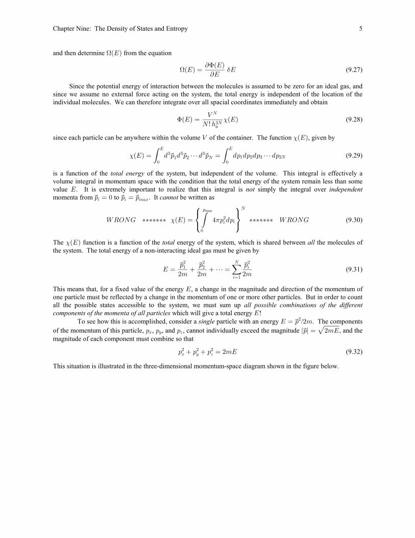
Figure 9.2 The phase space diagram for a one-dimensional simple harmonic oscillator of energy

I œ � 5B 2 œ B ::#7 #

" #9

#

. This figure also depicts the division of phase space into equal “cells” of size .$ $

The number of cells in phase space for the one-dimensional oscillator is given by the area of the ellipse divided by

the size of a cell, , or29

F1

ÐIÑ œ+,

29(9.14)

where

+ œ B œ #IÎ5

, œ : œ #7I

7+B

7+B

ÈÈ (9.15)

This gives

F1

=ÐIÑ œ

# I

29(9.16)

or, in the semi-classical approximation,

F 1 %1

=ÐIÑ œ œ # IÎ

# I

h(9.17)

To get an idea of the number of accessible states we are talking about, consider the case where the

frequency of oscillation is 1 kHz, eV-s, and is only 1.0 eV. In that case, Even2 œ 'Þ'$ ‚ "! I ÐIÑ ¸ "! Þ� "#15 Fwhen 1 MHz, ./ F¸ !! ÐIÑ ¸ "!(

Now for a three-dimensional oscillator, this would become

F1

%ÐIÑ œ I

#Π$$ (9.18)

and for such three-dimensional oscillators we haveR

F1

%ÐIÑ œ I

#Π$R$R (9.19)

provided the oscillators are distinguishable. This might be the case if the oscillators are fixed in location so that

individual oscillators do not move around and are therefore distinguishable by location.. If the oscillators are not

distinguishable, we again must divide this last equation by N! Either way, we see that is proportional to theFÐIÑnumber of degrees of freedom of the system (here there are 2 degrees of freedom for each dimension since the

energy of the oscillator has two quadratic terms: one for potential energy and one for kinetic energy). The

constant term in this last equation is different from that which we obtained for the free particle, but the

dependence of the number of cells on the total energy is the same - both vary as the total energy raised to the ÁÎ#power, where is the number of degrees of freedom of the system.Á

Chapter Nine: The Density of States and Entropy 4

The Number of States, , for an Ideal GasHÐIÑ . As we examine the number of states for an ideal gas, we

need first to look at the energy of the molecules which make up a gas. If we consider the case of a gas of Ridentical molecules enclosed in a container of volume , the total energy of the system, , is given byZ I

I œ O � Y �Iint (9.20)

The total kinetic energy of the system, , is due to the translational motion of the molecules, and is given byO

O œ OÐ: : á : œ :t t t t"

#7" #3œ"

R

3#, , , ) (9.21)n

where the 's are the translational momenta of each particle (which obviously changes whenever the molecules:t3collide with each other or with the walls of the container). The quantity r ,r , ,r ) represents the totalY œ YÐ át t t" # 8

potential energy of the system and is a function of the location . It is aof each and every particle of the system

function of the relative separations of all the particles, and, therefore, is constantly changing as the molecules

move around. We might, however, be able to find an expression for the potential energy in which theaverage

particles move.

If we assume that the molecules are not monatomic, each molecule can also rotate and vibrate relative to its

center of mass. The energy of this rotation and vibration we designate by , which is the internal energy of theIint

system diatomic(i.e., the sum of the internal energy of each individual molecule). An expression for for Iint

molecules might look something like

I œ � � �P

#M # #

" "†int o – —

3œ" 4œ"

R $4#

4

# # R (R R ) (9.22). ,

For an ideal, monatomic gas, with no interaction potential, the total energy of the system simplifies to give

I œ Ò: � : � : Ó œ + :"

#7 3œ" 4œ"

R R

B C D 4# # # #

4 (9.23)

3

where .+ œ "Î#74

We now want to determine the number of states, , for such an ideal gas with total energy lyingHÐIÑbetween and . To do this we again consider in which each coordinate, , is paired with aI I � I B$ phase space

momentum, , and we simply determine the number of in phase space with energy between and .: I I � IB cells $This could be done by integrating over all the coordinates and momenta of the system,accessible

HÐIÑ œ : : â : ; ; â ;"

Rx 2o$R

I

I� I

" # $R " # $R d d d d d d (9.24)($

where we have introduced in the denominator since the individual atoms of the ideal gas are indistinguishable.RxExpressing this last equation in terms of three-dimensional momenta and coordinates,

HÐIÑ œ : : â : < < â <"

Rx 2t t t t t t

o$R

I

I� I

$ $ $ $ $ $" # R " # R d d d d d d (9.25)(

$

where we have written d d d d and d d d d . This integral is difficult to perform because of$ $" 3B 3C 3D " 3 3 3: œ : : : < œ B C Dt t

the limitation on the energy. It is much simpler to proceed as we did earlier by evaluating the integral

FÐIÑ œ : : â : < < â <"

Rx 2t t t t t t

o$R

!

I

$ $ $ $ $ $" # R " # R d d d d d d (9.26)(

Chapter Nine: The Density of States and Entropy 5

and then determine from the equationHÐIÑ

H $F

ÐIÑ œ I` ÐIÑ

`I (9.27)

Since the potential energy of interaction between the molecules is assumed to be zero for an ideal gas, and

since we assume no external force acting on the system, the total energy is independent of the location of the

individual molecules. We can therefore integrate over all spacial coordinates immediately and obtain

F ;� � � �I œ IZ

Rx 2

R

$Ro

(9.28)

since each particle can be anywhere within the volume of the container. The function , given byZ I;� �;� � ( (I œ . : . : â. : œ .: .: .: â.:t t t

! !

I I$ $ $

" # R " # $ $R (9.29)

is a function of the of the system, but independent of the volume. This integral is effectively atotal energy

volume integral in momentum space with the condition that the total energy of the system remain less than some

value . It is extremely important to realize that this integral is simply the integral over I not independent

momenta from to . It be written as: œ ! : œ :t t t3 3 7+B cannot

[VSRK ‡‡‡‡‡‡‡ ÐIÑ œ % : .: ‡‡‡‡‡‡‡ [VSRK (9.30); 1

Ú ÞÛ ßÜ à(

!

:

3#

3

R3max

The function is a function of the energy of the system, which is shared between the molecules of;� �I total all

the system. The total energy of a non-interacting ideal gas must be given by

I œ � �â œ: : :t t t

#7 #7 #7

# # #" # 3

3œ"

R (9.31)

This means that, for a fixed value of the energy , a change in the magnitude and direction of the momentum ofIone particle must be reflected by a change in the momentum of one or more other particles. But in order to count

all the possible states accessible to the system, we must sum up all possible combinations of the different

components of the momenta of all particles which will give a total energy !I To see how this is accomplished, consider a particle with an energy / . The componentssingle I œ : #7t#

of the momentum of this particle, , , and , cannot individually exceed the magnitude , and the: : : l:l œ #7ItB C DÈ

magnitude of each component must combine so that

: � : � : œ #7IB C D# # # (9.32)

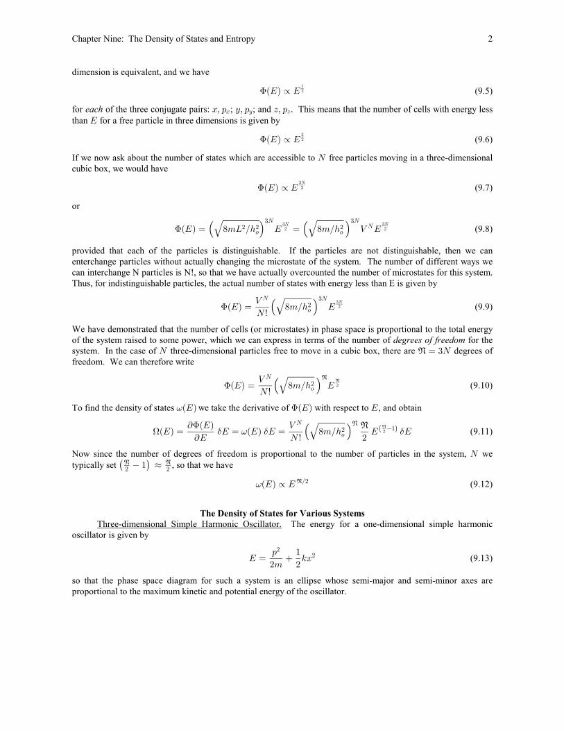
This situation is illustrated in the three-dimensional momentum-space diagram shown in the figure below.

Chapter Nine: The Density of States and Entropy 6

θ

φ

pz

py

px

p

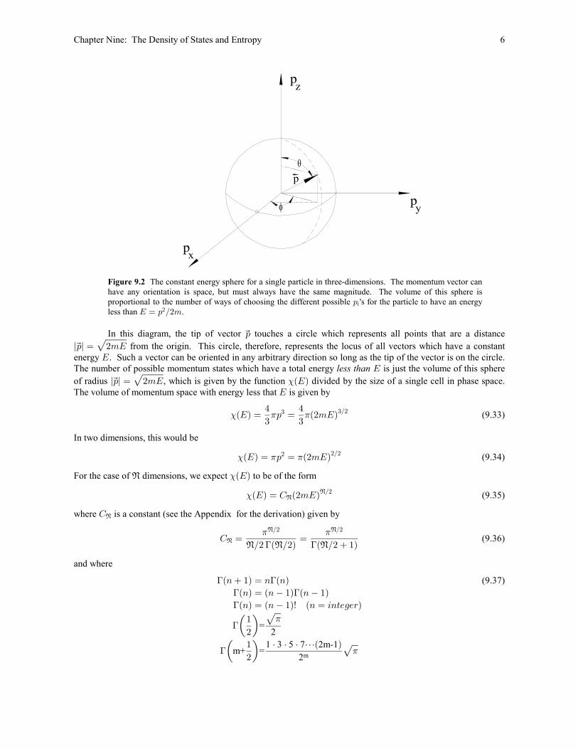
Figure 9.2 The constant energy sphere for a single particle in three-dimensions. The momentum vector can

have any orientation is space, but must always have the same magnitude. The volume of this sphere is

proportional to the number of ways of choosing the different possible 's for the particle to have an energy:3less than .I œ : Î#7#

In this diagram, the tip of vector touches a circle which represents all points that are a distance:t

l:l œ #7It È from the origin. This circle, therefore, represents the locus of all vectors which have a constant

energy . Such a vector can be oriented in any arbitrary direction so long as the tip of the vector is on the circle.IThe number of possible momentum states which have a total energy is just the volume of this sphereless than I

of radius , which is given by the function divided by the size of a single cell in phase space.l:l œ #7I It È � �;The volume of momentum space with energy less that is given byI

; 1 1� � � �I œ : œ #7I% %

$ $$ $Î#

(9.33)

In two dimensions, this would be

; 1 1� � � �I œ : œ #7I# #Î#(9.34)

For the case of dimensions, we expect to be of the formÁ ;� �I

;� � � �I œ G #7IÁÁÎ#

(9.35)

where is a constant (see the Appendix for the derivation) given byGÁ

G œ œÎ# Ð Î#Ñ Ð Î# � "Ñ

Á

Á Á1 1

Á > Á > Á

Î# Î#

(9.36)

and where

> >

> >

>

>1

> 1

Ð8 � "Ñ œ 8 8

8 œ 8 � " 8 � "

8 œ 8 � " x Ð8 œ 38>/1/<Ñ

"

#

" † † † â

#

� �� � � � � �� � � �Œ È

Œ � �È=

2

m+ =1 3 5 7 2m-1

2

(9.37)

m

Chapter Nine: The Density of States and Entropy 7

The total number of states in three-dimensions for monatomic atoms of an ideal gas is, therefore,Rgiven by

F ;ÐIÑ œ I œ G #7IZ Z

Rx 2 Rx 2

R R

$R $R $R$RÎ#

o o

� � � � (9.38)

Now to find the number of states between and , we differentiate with respect to I I � I I I$ F� �H $ $

FÐIÑ œ I œ G 7I #7 I

` ÐIÑ Z $R

`I Rx 2 # (2 ) (9.39)

R

$R $R$R # �"

o

/� �

or

H = $ $ÐIÑ œ ÐIÑ I œ G 7I #7 IZ $

ÐR � "Ñx 2 # (2 ) (9.40)

R

$R $R$R # �"

o

/� �

Just as before, in those cases where is very large, we can neglect the “ 1” term in the exponential, and in theR �factoral term in the denominator, giving

H = $ $ F $ÐIÑ œ ÐIÑ I œ G 7I 7 I œ ÐIÑ $7 IZ

Rx 2 (2 ) (3 ) (9.41)

R

$R $R$R #

o

/� � � �This last result is characteristic of those situations where is very large. In those cases, R the only difference

between , , and (E) is a relatively small constant we can work equally wellH F =ÐIÑ ÐIÑ . For that reason,

with , , or (E); but we usually work with , since it is easiest to calculate!H F = FÐIÑ ÐIÑ ÐIÑ And since isRof the order of Avogadro's number, we see that , , and (E) are all H F =ÐIÑ ÐIÑ extremely rapidly increasing

functions of the energy.

The Density of States and Equilibrium

Consider two systems and which are allowed to interact with each other thermally, but notE E" #

mechanically. (We also do not allow particle diffusion which we will be taken up later.)ß

A

A

1

2

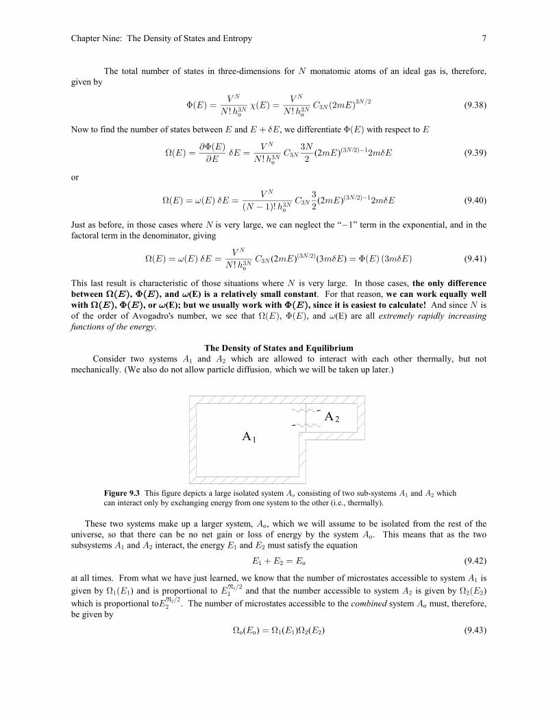
Figure 9.3 This figure depicts a large isolated system consisting of two sub-systems and whichE E E9 " #

can interact only by exchanging energy from one system to the other (i.e., thermally).

These two systems make up a larger system, , which we will assume to be isolated from the rest of theEo

universe, so that there can be no net gain or loss of energy by the system . This means that as the twoEo

subsystems and interact, the energy and must satisfy the equationE E I I" # " #

I �I œ I" # o (9.42)

at all times. From what we have just learned, we know that the number of microstates accessible to system isE"

given by ) and is proportional to and that the number accessible to system is given by )H H" " # # #"Î#

ÐI I E ÐIÁ"

which is proportional to . The number of microstates accessible to the system must, therefore,I E#ÎÁ# 2

ocombined

be given by

H H Ho o( ) ( ) ( ) (9.43)I œ I I" " # #

Chapter Nine: The Density of States and Entropy 8

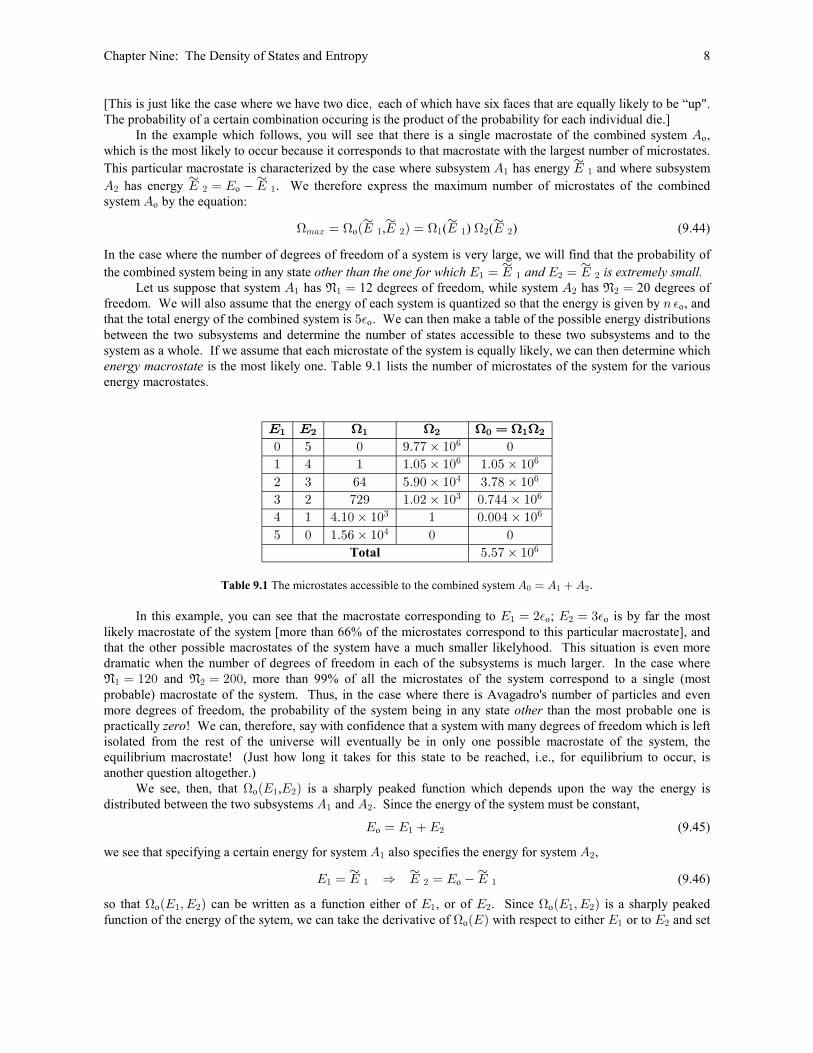
[This is just like the case where we have two dice each of which have six faces that are equally likely to be “up".ßThe probability of a certain combination occuring is the product of the probability for each individual die.]

In the example which follows, you will see that there is a single macrostate of the combined system ,Eo

which is the most likely to occur because it corresponds to that macrostate with the largest number of microstates.

This particular macrostate is characterized by the case where subsystem has energy and where subsystemE Iµ

" "

E I œ I �Iµ µ

# # " has energy . We therefore express the maximum number of microstates of the combinedo

system by the equation:Eo

H H H H7+B " # " " # #œ ÐI I Ñ œ I Iµ µ µ µ

o , ( ) ( ) (9.44)

In the case where the number of degrees of freedom of a system is very large, we will find that the probability of

the combined system being in any state other than the one for which and is extremely small.I œ I œ" " # #I Iµ µ

Let us suppose that system has 12 degrees of freedom, while system has 20 degrees ofE œ E œ" " # #Á Áfreedom. We will also assume that the energy of each system is quantized so that the energy is given by , and8 %othat the total energy of the combined system is . We can then make a table of the possible energy distributions&%obetween the two subsystems and determine the number of states accessible to these two subsystems and to the

system as a whole. If we assume that each microstate of the system is equally likely, we can then determine which

energy macrostate is the most likely one. Table 9.1 lists the number of microstates of the system for the various

energy macrostates.

I I œ" # " # ! " #H H H H H

! & ! *Þ(( ‚ "! !

" % " "Þ!& ‚ "! "Þ!& ‚ "!

# $ '% &Þ*! ‚ "! $Þ() ‚ "!

$ # (#* "Þ!# ‚ "! ! (%% ‚ "!

% " %Þ"! ‚ "! " !Þ!!% ‚ "!

& ! "Þ&' ‚ "! ! !

&Þ&

'

' '

% '

$ '

$ '

%

.

Total ( ‚ "!'

Table 9.1 The microstates accessible to the combined system E œ E �E Þ! " #

In this example, you can see that the macrostate corresponding to ; is by far the mostI œ # I œ $" #% %o o

likely macrostate of the system [more than 66% of the microstates correspond to this particular macrostate], and

that the other possible macrostates of the system have a much smaller likelyhood. This situation is even more

dramatic when the number of degrees of freedom in each of the subsystems is much larger. In the case where

Á Á" #œ "#! œ #!! and , more than 99% of all the microstates of the system correspond to a single (most

probable) macrostate of the system. Thus, in the case where there is Avagadro's number of particles and even

more degrees of freedom, the probability of the system being in any state than the most probable one isother

practically ! We can, therefore, say with confidence that a system with many degrees of freedom which is leftzero

isolated from the rest of the universe will eventually be in only one possible macrostate of the system, the

equilibrium macrostate! (Just how long it takes for this state to be reached, i.e., for equilibrium to occur, is

another question altogether.)

We see, then, that , is a sharply peaked function which depends upon the way the energy isHoÐI I Ñ" #

distributed between the two subsystems and . Since the energy of the system must be constant,E E" #

I œ I �Io " # (9.45)

we see that specifying a certain energy for system also specifies the energy for system ,E E" #

I œ I Ê I œ I �Iµ µ µ

" " # " (9.46)o

so that can be written as a function either of , or of . Since is a sharply peakedH Ho oÐI ßI Ñ I I ÐI ßI Ñ" # " # " #

function of the energy of the sytem, we can take the derivative of with respect to either or to and setHoÐIÑ I I" #

Chapter Nine: The Density of States and Entropy 9

this equal to zero to determine the most likely values or :I Iµ µ

" #

º ºd ( , ) d ( , )

d d 0 or 0 (9.47)

H Ho oI I I I

I Iœ œ

" # " #

" #I Iµ µ

" #

The Density of States, Temperature, and Entropy

If the two subsystems are in equilibrium with each other, the temperature of one subsystem is differentnot

from that of the other, and the energies and will be changing toward the equilibrium values and .I I I Iµ µ

" # " #

As we demonstrated in the last section, we expect that the equilibrium condition, the state toward which the two

subsystems will move, corresponds to that in which the number of states available to the system as a whole will

increase increase. In other words, we expect , ) to with changing and until the maximum valueHoÐI I I I" # " #

H H HoÐI I Ñ œ I Iµ µ µ µ

" # " " # #, ( ) ( ) is reached. Thus, we expect heat to flow from one system into the other until the

systems come to equilibrium. It would seem that our statistical arguments must give the observed result that heat

always flows from a hotter system to a cooler system. This prefered direction of heat flow is associated with the

entropy change of the system.

We have found that the macrostate (and its corresponding parameters) which maximizes the number of

microstates of the combined system is given by ( , where H H Ho I ßI Ñ œ ÐI Ñ ÐI ѵ µ µ µ

" # " " # # the number of

microstates of the combined system is the of the microstates of the individual subsystemsproduct . The fact that

we must consider a of the microstates of the two systems is in contrast to other parameters of the twoproduct

subsystems, such as the energy, the volume, and the number of particles which are To create a littleadditive.

more similarity with these other parameters of the subsystems, we notice that the log of the number of microstates

of the subsystems additiveis , or:

ln ln ln (9.48)H H HoÐI ßI Ñ œ ÐI Ñ � ÐI ѵ µ µ µ

" # " " # #

We therefore define a quantity called “entropy” by the equation

WÐIÑ œ 5 ÐIÑln (9.49)H

where (Boltzmann's constant) is just a scaling factor. With this definition we can write5

W ÐI ßI Ñ œ W ÐI Ñ � W ÐI Ño " # " " # # (9.50)

for the combined system . Notice that a change in can be writtenE Wo o

.W ÐI ßI Ñ œ .I � .I`W ÐI Ñ `W ÐI Ñ

`I `Io " # " #

" " # #

" # (9.51)

But the energy change is related to the energy change by the equation.I .I" #

.I � .I œ .I œ ! Ê .I œ � .I" # " #o (9.52)

so that the change in can also be written asW ÐIÑo

.W ÐI ßI Ñ œ .I � .I œ � .I`W ÐI Ñ `W ÐI Ñ `W ÐI Ñ `W ÐI Ñ

`I `I `I `Io " # " " "

" " # # " " # #

" # " # (9.53)œ

Now, in the case where we evaluate this change at the most likely values of and (which we designate byI I" #

I I ÐIÑ W œ 5 ÐIѵ µ

" # and ), we know that and therefore ln[ ] is a , givingH Ho o maximum

k Ÿ.W œ œ � .I`W ÐI Ñ `W ÐI Ñ

µ µ

`I `Io Iµ

" " # #

" #"

"0 (9.54)

The previous equation indicates that the maximum entropy of the combined system is obtained only when

º º`W ÐI Ñ `W ÐI Ñ

`I `Iœ

" " # #

" #I Iµ µ

" #

(9.55)

Chapter Nine: The Density of States and Entropy 10

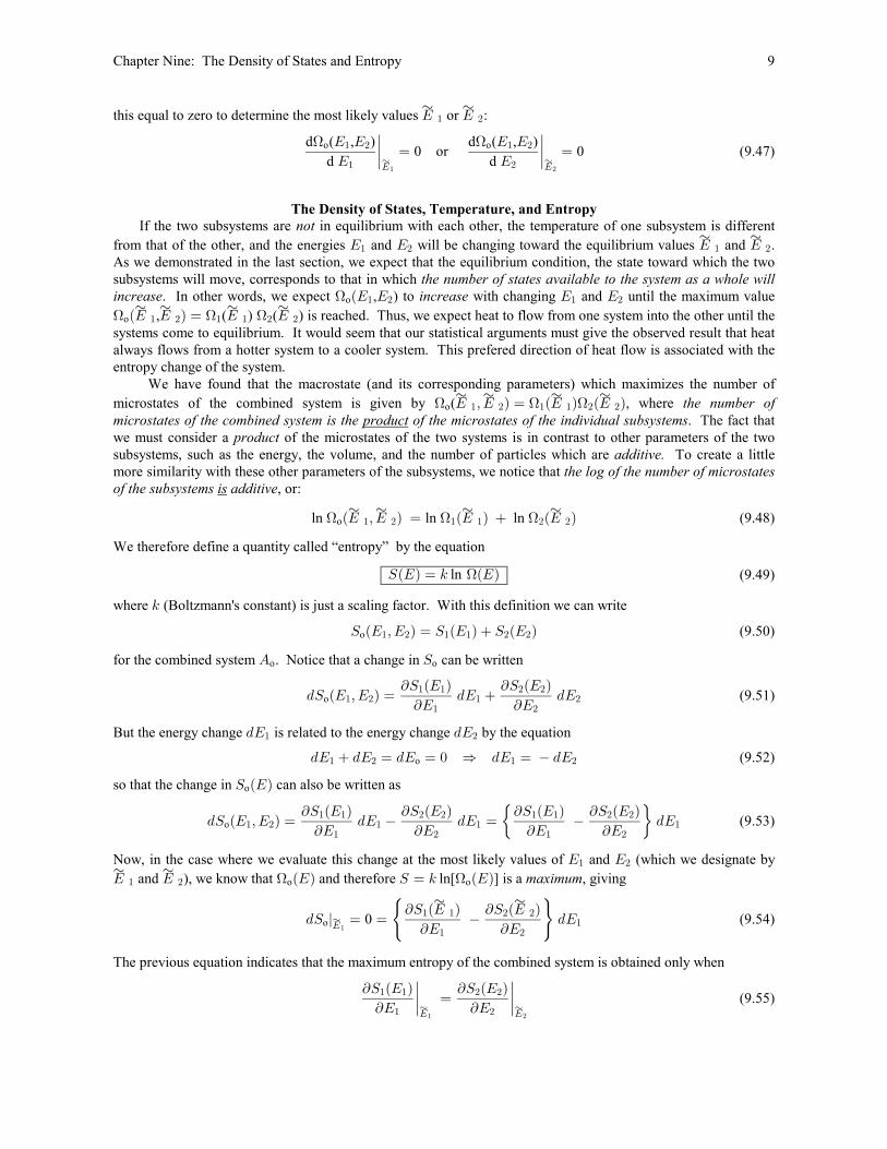
Notice that the left hand side of this equation is only a function of system while the right hand side is only aE"

function of system ! This last equation would seem to imply that the partial of with respect to energy,E W#

evaluated at the equilibrium energy, must be related to the temperature, for it is the temperature of two adjacent

systems which is equal when they come to equilibrium. In fact, you should recall that this is just the definition of

the temperature - that thermometric property which determines when two systems are in thermal equilibrium!

`W`I

9

"œ !

So

E

E

1

2

Figure 9.4 The entropy of the combined system plotted against the energy of each subsystem

To see just how the partial derivative of the entropy with respect to energy of a system is related to the

temperature, let us look back at the general expression for the number of states of the system with energy ,Iwhich we designated . We found that a general expression for the number of states for an ideal gas is givenHÐIÑby the equation

H = $ F $ÐIÑ œ ÐIÑ I œ ÐIÑ $7 I (9.56)� �The entropy, then can be written as

WÐIÑ œ 5 ÐIÑ œ 5 I � I œ 5 ÐIÑ � Ð$7 IÑln ln ln ln ln (9.57)H = $ F $c d c d� �So we see that the entropy can be expressed as

WÐIÑ œ 5 ÐIÑ

WÐIÑ œ 5 ÐIÑ

WÐIÑ œ 5 ÐIÑ

ln (9.58)

ln

ln

c dc dc dH

=

F

to within some arbitrary constant! In most cases, we will simply ignore the constant, and use whichever of these

expressions is easiest to calculate [usually the one with ].FÐIÑ Thus, the entropy for a three-dimensional ideal gas is given by

WÐIÑ œ 5 I œ 5 #7IZ

Rx 2 Ð$RÎ# � "Ñln ln (9.59)F

1

>� � � � ŸR $RÎ#

$R

$RÎ#

o

WÐIÑ œ 5 � R R �R � � � � #7IZ $R $R $R

2 # # # ŸŒ ” •c d ˆ ‰ Œ ln ln ln ln ln( ) (9.60)o$

R$RÎ# $RÎ#1

Chapter Nine: The Density of States and Entropy 11

This can be written as

WÐIÑ œ 5 � R R �R � � � � #7IZ $R $R

2 # # ŸŒ Œ ˆ ‰ln ln ln ln ln( ) (9.61)o$

R $RÎ#$RÎ# $RÎ#1

or combining the middle terms, we can writeß

WÐIÑ œ 5 � R R � � � #7IZ # &R

2 $R # ŸŒ Œ ln ln ln ln( ) (9.62)o$

R $RÎ#$RÎ#1

In this last expression we have several ln terms raised to the N power. This can be written asth

WÐIÑ œ 5 R �R R �R � �R #7IZ # &R

2 $R # ŸŒ Œ ln ln ln ln( ) (9.63)o$

$Î#$Î#1

and we can factor the N out of the equation to obtain

WÐIÑ œ R5 � R � � � #7IZ # &

2 $R # ŸŒ Œ ln ln ln ln( ) (9.64)o$

$Î#$Î#1

This can be further simplified to give

WÐIÑ œ R5 � �Z % 7I &

R2 $R #œ Œ ln ln( ) (9.65)

o$

$Î#1

or, finally,

WÐIÑ œ R5 68 �Z % 7I &

R $R2 # Ÿ– —Œ Œ 1#9

$Î#

(9.66)

which is the equation. This equation has been experimentally verified as the correct entropy ofSakur-Tetrode

an ideal gas at high tempereatures, if is numberically set equal to Plank's constant. Another form of this29equation can be written by recognizing that we can write

&

#œ /ln (9.67)&Î#

Using this we can write the Saku-Tetrode equation in the form

WÐIÑ œ R5 68 /Z % 7I

R $R2 Ÿ– —Œ Œ &Î##9

$Î#1

(9.68)

Now, the partial of with respect to energy is given byW

Œ Ú ÞÝ áÛ ßÝ áÜ à

’ “� �� � � �`WÐIÑ $

`I #œ R5 œ R5 "ÎI

I

IZ ßR

..I

$Î#

$Î# (9.69)

where we have specifically indicated that the volume and the number of particles remains constant. Solving the

the energy, we obtain

I œ ‚$R 5 `WÐIÑ

# `I Ÿ„Œ 1 (9.70)Z ßR

Chapter Nine: The Density of States and Entropy 12

From the equipartition theorem, we know that the energy of a three-dimensional ideal gas is given by

I œ 5X œ 5XR

# #

3(9.71)

Á

so we see that the change in entropy with respect to energy must be the inverse of the absolute temperature:

ˆ ‰`W "`I XZ ßR

œ (9.72)

Note: It is interesting to notice that the temperature of a system is proportional to the average

energy per degree of freedom ( ) of a system, and that two systems come to equilibrium whenIÎÁthis average energy is equal.

Thus, Equ. 9.55 simply states that two systems and in thermodynamic equilibrium, must have theE E" #

same temperature:

" "

X Xœ X œ X

" #" # or (9.73)

Entropy, Heat Flow and the Second Law of Thermodynamics

For our combined system , the number of microstates accessible is given byEo

H H Ho o( ) ( ) ( ) (9.74)I œ I I" " # #

so that the entropy of the combined system is given by

W ÐI Ñ œ W ÐI Ñ � W ÐI Ño o " " # # (9.75)

since ln[ ]. When the system comes to equilibrium, the combined system is in a macrostate whichW œ 5 ÐIÑHcorresponds to the maximum number of microstates, and, therefore, the maximum value of the entropy:

W œ W ÐI I œ W I � W Iµ µ µ µ

max o " # " " # #, ) ( ) ( ) (9.76)

But what happens when the system is in equilibrium? In this case we have two system and not E E" #

which are both isolated and independently in a state of thermodynamic equilibrium. When we bring these two

systems in contact with one another, and allow them to interact thermally, the combined system is not initiallyE9

in its most probable configuration, and so the two systems exchange energy in such a way that the entropy of the

entire system We know that this must be true because the equilibrium condition arises when theincreases.

entropy of the combined system is a maximum. Thus, when two systems are brought in thermal contact with one

another, the total entropy of the combined system either increase or (if the two systems are already inmust

equilibrium with each other) remain constant:

.W I I   !o( , ) for isolated systems (9.77)" #

The fact that the entropy of an isolated sytem must increase or remain constant is one expression of the second

law of thermodynamics. As a natural consequense of this we find that

.W œ .I � .I   !`W `W

`I `Io

" #

" #" # (9.78)

but the conservation of energy requires that

.I œ � .I" # (9.79)

which gives

.W œ .I � .I œ � .I   !`W `W `W `W

`I `I `I `Io

" # " #

" # " #" " " (9.80)œ

Chapter Nine: The Density of States and Entropy 13

or

œ " "

X X� .I   !

" #" (9.81)

This equation tells us that if , i.e, if energy is flowing subsystem , then the term in brackets must.I I ! E" "into

also be greater than zero, which implies that ! Similarly, if , i.e., if energy is subsystemX I X .I � !# " " leaving

E X I X" " #, then the term in the brackets must also be negative, which implies that ! This is consistent with our

experience and is another way of stating the second law of thermodynamics: energy flows spontaneously from

hotter objects into cooler objects and not vice versa!

Notice that what we have said so far indicates that it is the entropy of the which mustcombined system

increase when two systems interact with each other. The entropy of individual subsystems may either increase or

decrease. You can see that this is true by looking back at Table 7.1. The maximum number of microstates (the

maximum entropy) of the combined system does not correspond to the maximum number of microstates for either

of the subsystems. If the two systems are not initially in equilibrium, then the systems will transfer energy is such

a was as to give the maximum number of microstates for the combined system. One of the subsystems will loose

energy (decreasing the number of microstates accessible to that subsystem) while the other will gain energy

(increasing the number of microstates accessible to that subsystem).

Entropy and the Third Law

The entropy is defined by the equation ln , or ln and we have shown that theW œ 5 Ð W œ 5 � -98=>ÞÑH Fnumber of states accessible to a system is a rapidly increasing function of the energy. But what happens as the

energy of the system ? Now the temperature of a system is a measure of the average energy per degreedecreases

of freedom. As the energy of a system decreases, the number of microstates accessible to the system dramatically

decrease. In fact, as the energy of the system decreases more and more the energy approaches the ground state

energy of the system. In the case where the ground state is non-degenerate, there is only one state of the system

for the system's lowest energy, which means that the entropy of this state of the system is given by

W œ 5 Ð"Ñ œ !9 ln (9.82)

Even in the case where the ground state energy degenerate, the number of states accessible to the systemis

becomes quite small, so that the entropy of that state of the system is extremely small in comparison to the

entropy of higher energy states. It is instructive to note that the lower limit to the entropy is purely a quantum

mechanical concept.

The Calculation of the Entropy and Changes in Entropy

The Sakur-Tetrode equation for the entropy of an ideal gas is given by

WÐIÑ œ R5 68 �Z % 7I &

R $R2 # Ÿ– —Œ Œ 1#9

$Î#

(9.83)

where the entropy is clearly a function of the number of particles, the volume, and the energy of the system.

(Note: In particular, note that the entropy is a function of the and the .)volume per particle energy per particle

The change in entropy can be expressed by the equation.W

.W œ .I � .Z � .R`W `W `W

`I `Z `RŒ Œ Œ

Z ßR IßR Z ßI

(9.84)

Now, if we hold the number of particles and the volume of the system constant, the change in entropy of the

system is due only to an energy transfer in the form of heat (i.e., Q if the energy change in only in the.I œ $form of heat) In this case we can writeÞ

.W œ U œ`W U

`I XŒ

Z ßR

$$

(9.85)

Chapter Nine: The Density of States and Entropy 14

This last equation is valid for infintesimal quasi-static transfer of heat energy any no matter how large or small

the system the change in the entropy of a system. This means that can be determined from the equation

?$

W œU

X(/;

(9.86)

where we have explicitly indicated that the process must be carried out . It is important to noticequasi-statically

that although the amount of heat, , added to (or removed from) a system depends upon the process, when we$Udivide by the absolute temperature, , of the system X at each point along the equilibrium surface of the process

(which will generally change from point to point), we obtain the exact differential of the entropy . The fact.Wthat the entropy is a state variable can be easily seen in that it is related to the number of microstates accessible to

the system which has a unique value depending upon the parameters of that system.

Fluctuations about the Equilibrium Temperature

Since the entropy of a system is based upon probabilities, and since all microstates of a combined system

are equally likely, is it not possible for the system to move from the state of equilibrium, since such aaway

microstate of the system surely exists? If this possible, then we have the situation where the entropy of anis

isolated system actually (and heat spontaneously flows from cold objects into hot objects)! To answerdecreases

this question, we want to examine the likelyhood of fluctuations about the maximum value of the entropy of the

system. This is the same thing as looking at the dispersion of the probability distribution to determine the

likelyhood of seeing occurances other than the average. Let's examine the probability that a subsystem has anE"

energy , close to the equilibrium energy . Now the number of states accessible to this subsystem is relatedI Iµ

" "

to the entropy ln . We will express this function in terms of a Taylor series about the point ofW œ 5 Ò ÐI ÑÓ" "Hmaximum entropy and obtain:

ln ln (9.87) ln

+ ) ln

Ò ÐI ÑÓ œ Ò ÐI ÑÓ � ÐI � I ѵ µ` Ò ÐI ÑÓ

`I

" ` Ò ÐI ÑÓ

#x `IÐI � I �â

µ

H HH

H

" " " ""

" Iµ

#"

"#

Iµ

" "#

ºŒ ºŒ

"

"

(we have divided each term of this expansion by ). We will write this equation in the more simplified form:5

ln ln (9.88)Ò ÐI ÑÓ œ Ò ÐI ÑÓ � � �âµ "

#xH H " ( - (" " " "

#

where ( , and , defined so that . Likewise, we( " - -œ I �I Ñ œ œ œ � I !µ

" " " ""5X `I `I

` Ò ÐI ÑÓ

Iµ

`Iµ

" "

"

""

¹Š ‹ ¸ˆ ‰ ln H "

will expand ln about to obtainÒ ÐI ÑÓ Iµ

H # #

ln ln ln

) ln

Ò ÐI ÑÓ œ Ò ÐI ÑÓ � ÐI � I ѵ µ` Ò ÐI ÑÓ

`I

� ÐI � I �â" ` Ò ÐI ÑÓ

# `I

µ

H HH

H

# # # ##

# Iµ

##

##

Iµ

# ##

ºŒ ºŒ

#

#

or (9.89)

ln ln (9.90)Ò ÐI ÑÓ œ Ò ÐI ÑÓ � Ð � Ñ � Ð � Ñ �âµ "

#H H " ( - (# # # #

#

Note that the energy differences, , are opposite in sign, since the total energy of the system must remain fixed, so(

that ( , and .( ( ( (" " " # # #œ I �I Ñ œ œ ÐI � I Ñ œ �µ µ

The number of states for the system is found by adding these two equations together to get:combined

ln ln ( ) (9.91)Ò ÐI Ñ ÐI ÑÓ œ Ò ÐI Ñ ÐI ÑÓ � Ð � Ñ � � �âµ µ "

#H H H H " " ( - - (" # " # " # " #

#

Chapter Nine: The Density of States and Entropy 15

Now, at the point where and , we see that , so that the term linear in goes to zero,I œ I I œ I œµ µ

" " # # " #" " (leaving

ln ln ( (9.92)c c -ÐIÑ œ ÐI Ñ � I � I ѵ µ"

#o

#

or

c c -ÐIÑ œ ÐI Ñ /B:Ò � ÐI � I Ñ Óµ µ"

# (9.93)o

#

where we have define , and where is the probability of finding one of the subsystems (in this- - - co œ � ÐIÑ" #

particular calculation, ) with an arbitrary energy . We notice that the probability of measuring a particularI I"

energy is a Gaussian function which is peaked about the , , and that the standard deviation ofI Iµ

average energy

this Gaussian is given by . Central to this conclusion is the requirement that is5 - - - -#" # 3œ "Î œ "ÎÐ � Ño

positive. To demonstrated this, remember that . This givesH º IÁÎ#

"H Á Á

œ œ œ` ` I

`I # `I #I

ln ln (9.94)

and

-" Á

œ � œ � � I`

`I #I 0 (9.95)Π#

Now, since 66% of all states lie within of the average value, the question we need to answer is just how„ 5large an enegy change in one of the subsystems will give one standard deviation in the probability function. The

standard deviation is given by

5-

œ"È

o

, (9.96)

where

- - - - -- -

- -o œ � œ " � œ " �" # " #

# "

" #œ œ (9.97)

Notice that if , ; while if ; and if , . Thus, let - - - - - - - - - - - - - Á" # " # " # " # "#¦ ¶ ¦ ß ¶ ¶ ¶ # ¶ Î#Io o o � �

be equal to the of , orlargest -3

5- Á

œ ¶ I" #È Ê

o

(9.98)

If we let be the energy fluctuation equal to one standard deviation, then , and for systems with a?I ¶5?

ÁII

#5 Élarge number of degrees of freedom (say ), the percentage fluctuation in energy is of the order of %."! "!#! �)

Thus we expect only fluctuations about the equilibrium states of the system, so that to a goodvery small

approximation, once the system reaches equilibrium, the parameters of the system remain essentially constant.

Summary

In summary, then, we find that when two systems interact with one another, the macroscopic parameters

of the two systems change in such a way as to increase the entropy Ðthe number of microstates) of the combined

system, and the equilibrium values of these parameters are those for which the entropy is a maximum! And once

the equilibrium parameters of a system are reached, these equilibrium parameters remain constant to a precision

greater than we normally can measure. It is important to notice that the entropy of individual subsystems may

increase decrease, and that our conclusions are based upon the assumption that the composite system or isEo

isolated from the rest of the universe. For anyTherefore, the second law of thermodynamics should be stated:

isolated system, the entropy of the system will always increase or remain the same!

APPENDIX 9.1

INTERNAL ENERGY OF A NON-IDEAL GAS

If we consider the case of a gas of identical molecules enclosed in a container of volume , the energy ofR Zthe system is given by

I œ O � Y �Iint (A9.1.1)

where is the total energy of the system. The total kinetic energy of the system, , is due to the translationalI Omotion of the molecules, and is given by

O œ OÐ: : á : œ :t t t t"

#7" #3œ"

R

3#, , , ) (A9.1.2)n

where the 's are the translational momenta of each particle (which obviously changes whenever the molecules:t3collide with each other or with the walls of the container). The quantity r ,r , ,r ) represents the totalY œ YÐ át t t" # 8

potential energy of the system and is a function of the location . It is aof each and every particle of the system

function of the relative separations of all the particles, and, therefore, is constantly changing as the molecules

move around. Since we did not assume that the molecules were monatomic, each molecule can also rotate and

vibrate relative to its center of mass. The energy of this rotation and vibration we designate by , the internalIint

energy of the system which is the sum of the internal energy of each individual molecule. An expression for Iint

for diatomic molecules might look something like

I œ � � �P

#M # #

" "†int o – —

3œ" 4œ"

R $4#

4

# # R (R R ) (A9.1.3). ,

Typically, we designate the (linear momentum, angular momentum, etc.) relative to thegeneralized momenta

center of mass of the molecule by , , , , and the corresponding (theT T á T" # 7 generalized coordinates

internuclear distance, the angles of rotation, etc.) by , , , . Thus, a general expression for the internalU U á U" # 7

energy of the system might be

I œ T � Uint – —ˆ ‰3œ" 4œ"

R 7

4 44 4# # (A9.1.4)α "

where the 's and 's are constants (some of which may be zero).α " Now if we denote the generalized momenta of the center of mass of individual molecules by , , and: : :" # $,

corresponding generalized coordinates of the center of mass of the individual molecules by , , , we can write; ; ;" # $

the total energy of the system as

I œ + : � , ; � I – —ˆ ‰3œ" 4œ"

R $

4 44 4# # (A9.1.5)int

where the 's and 's are constants (some of which may be zero). However, it is customary to simply number each+ ,momentum variable, , and its constant from to , and correspondingly, each coordinate variable, ,: + 4 œ " $R ;4 4 4

and its constant from to , giving, 4 œ " $R4

I œ + : � , ; � I ˆ ‰4œ"

R

4 44 4# #

3

int (A9.1.6)

In some cases of interest, this equation can be greatly simplified. In the case of monatomic gasses, for

example, the internal energy, , is zero. Likewise, for the case where the intermolecular distances are large onIint

average the potential energy of interaction is negligible. This implies that the total energy is independent of the

Chapter Nine: The Density of States and Entropy 17

coordinates, , of the center of mass, and that the total energy of the system can be expressed by;4

I œ + :4œ"

R

4 4#

3

(A9.1.7)

This is the so-called “ideal gas" approximation.

To determine the number of states for a non-ideal gas, we simply “add up" all the states between theHÐIÑenergy and by integrating over all the accessible coordinates and momenta of the system. This isI I � I$equivalent to integrating over all accessible volume elements in phase space, or, in general,

HÐIÑ º : : â : ; ; â ; T T â T U U â U(I

I� I

" # $R " # $R " # 7 " # 7

$

d d d d d d d d d d d d (A9.1.8)

or, expressed in terms of three-dimensional momenta and coordinates,

HÐIÑ º : : â : < < â < T T â T U U â Ut t t t t t(I

I� I

$ $ $ $ $ $" # R " # R " # 7 " # 7

$

d d d d d d d d d d d d (A9.1.9)

where we have written d d d d and d d d d . In fact, what we do is to evaluate the integral$ $" 3B 3C 3D " 3 3 3: œ : : : < œ B C Dt t

FÐIÑ º : : â : < < â < T T â T U U â Ut t t t t t(!

I

$ $ $ $ $ $" # R " # R " # 7 " # 7d d d d d d d d d d d d (A9.1.10)

and then determine from the equationHÐIÑ

H $F

ÐIÑ œ I` ÐIÑ

`I (A9.1.11)

For those cases in which the potential energy of interaction is negligible, the total energy is independent of

the intermolecular distances, and, therefore, of the coordinates of the molecules. This means that since the energy

is not a function of the coordinates, we can immediately integrate over all values of the coordinates accessible to

the molecules (the energy doesn't restrict which values of the coordinates we can integrate over). Each integral

over just gives the volume accessible to molecule , so that we have< 3t3

( d (A9.1.12)$3< œ Zt

for each particle in the system. This means that the number of states must be given by

F ;ÐIÑ º Z ÐIÑR (A9.1.13)

where

;ÐIÑ œ : : â : T â T U â Ut t t(0

I

$ $ $" # R " Q " Qd d d d d d d (A9.1.14)

is independent of the volume , since neither nor depend upon the coordinates .Z O I <tint 3

APPENDIX 9.2

EVALUATION OF THE INTEGRATING CONSTANT FOR AN -DIMENSIONAL SPACE8

As pointed out in the body of the chapter, the number of states available to an ideal gas with energy

ranging from to is given by the integral! I

FÐIÑ œ : : â : < < â <"

2t t t t t t

o$R

!

I

$ $ $ $ $ $" # R " # R d d d d d d (A9.2.1)(

from which we can determine from the equationHÐIÑ

H $F

ÐIÑ œ I` ÐIÑ

`I (A9.2.2)

Since the potential energy of interaction between the molecules is zero for an ideal gas, and since we

assume no external force acting on the system, the total energy is independent of the location of the individual

molecules so that we can perform the integration over spacial coordinates immediately to obtain

F ;ÐIÑ œ ÐIÑZ

2

R

$Ro

(A9.2.3)

since each particle can be anywhere within the volume of the container. The function is given byZ ÐIÑ;

;ÐIÑ œ : : â : œ .: .: .: .: â.:t t t( (! !

I I

$ $ $" # R " # $ % $Rd d d (A9.2.4)

and is a function of the of the system, but independent of the volume. This integral is effectively atotal energy

volume integral in momentum space with the condition that the total energy of the system remain less than some

value I, which is given by

I œ � �â œ: : :

#7 #7 #7

t t t" # 3# # #

3œ"

R (A9.2.5)

This means that, for a fixed value of the total energy of the system, a change in the magnitude of theImomentum of one particle must be reflected by a change in momentum of one or more other particles. But in

order to count all the possible states accessible to the system, we must sum up all possible combinations of the

different momenta which will give a total energy !I This situation is illustrated in the diagram of three-dimensional space shown in Figure A7.1. In this

diagram the tip of vector touches a circle which represents all points that are a distance from the: l:l œ #7It Èorigin. This circle, therefore, represents the locus of all vectors which have the constant energy . Such a vectorIcan be oriented in any arbitrary direction so long as the tip of the vector is on the circle. The number of possible

momentum states which have a total energy must be proportional to the volume of this sphere of radiusless than E

l:l œ #7I IÈ . The volume of momentum space with energy less than is given by

; 1 1ÐIÑ œ : œ #7I% %

$$ $Î#

3(A9.2.6)� �

In two dimensions, this would be

; 1 1ÐIÑ œ : œ #7I# � �2/2(A9.2.7)

For the case of dimensions, we expect to be of the formÁ ;ÐIÑ

;ÐIÑ œ G #7IÁÁ� � Î#

(A9.2.8)

where is some constant which we want to evaluate.GÁ

Chapter Nine: The Density of States and Entropy 19

θ

φ

pz

py

px

p

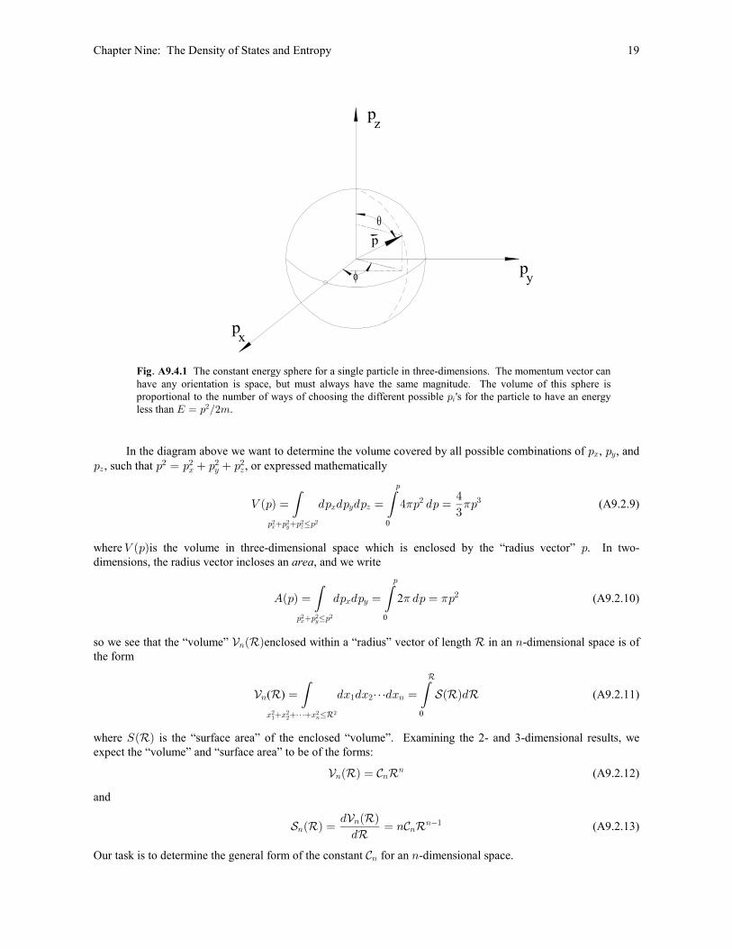
Fig A9.4.1Þ The constant energy sphere for a single particle in three-dimensions. The momentum vector can

have any orientation is space, but must always have the same magnitude. The volume of this sphere is

proportional to the number of ways of choosing the different possible 's for the particle to have an energy:3less than .I œ : Î#7#

In the diagram above we want to determine the volume covered by all possible combinations of , , and: :B C

: : œ : � : � :D# # # #

B C D, such that , or expressed mathematically

Z Ð:Ñ œ .: .: .: œ % : .: œ :%

$( (

: �: �: Ÿ:

B C D

:

# $

B C D# # # # 0

1 1 (A9.2.9)

where is the volume in three-dimensional space which is enclosed by the “radius vector” . In two-Z : :� �dimensions, the radius vector incloses an , and we writearea

EÐ:Ñ œ .: .: œ .: œ :( (: �: Ÿ:

B C

:

#

B C# # # 0

2 (A9.2.10)1 1

so we see that the “volume” enclosed within a “radius” vector of length in an -dimensional space is ofi e e8Ð Ñ 8the form

i e f e e8 " # 8

B �B �â�B Ÿ

( ) (A9.2.11)œ .B .B â.B œ Ð Ñ.( (" ## #

8# #e

e

0

where is the “surface area” of the enclosed “volume”. Examining the 2- and 3-dimensional results, weWÐ Ñeexpect the “volume” and “surface area” to be of the forms:

i e V e8 88Ð Ñ œ (A9.2.12)

and

f e V ei e

e8 8

8 8�"Ð Ñ œ œ 8. Ð Ñ

.(A9.2.13)

Our task is to determine the general form of the constant for an -dimensional space.V8 8

Chapter Nine: The Density of States and Entropy 20

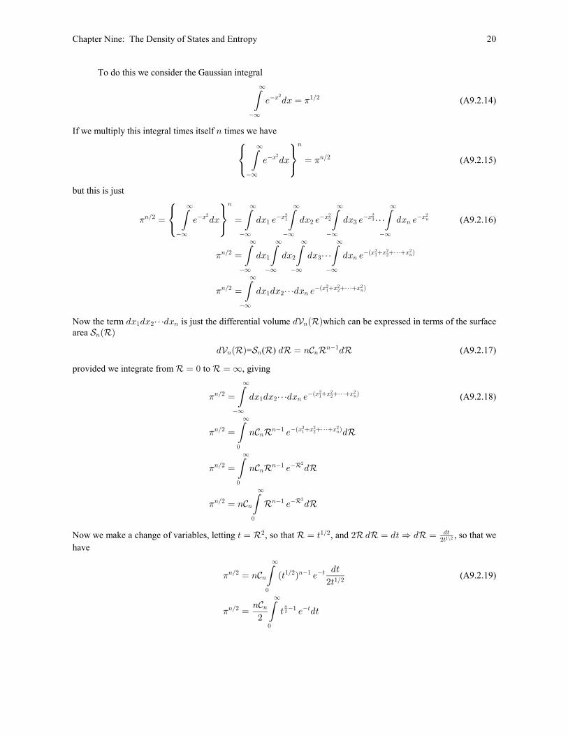
To do this we consider the Gaussian integral

(�∞

∞

�B "Î#/ .B œ#

1 (A9.2.14)

If we multiply this integral times itself times we have8

Ú ÞÛ ßÜ à(

�∞

∞

�B 8Î#

8

/ .B œ#

1 (A9.2.15)

but this is just

1

1

1

8Î# �B �B �B �B �B

�∞ �∞ �∞ �∞ �∞

∞ ∞ ∞ ∞ ∞8

" # $ 8

8Î# �ÐB �B �â�B Ñ

�∞ �∞ �∞ �∞

∞ ∞ ∞ ∞

" # $ 8

8Î#

œ / .B œ .B / .B / .B / â .B /

œ .B .B .B â .B /

œ

Ú ÞÛ ßÜ à( ( ( ( (

( ( ( (

# # # # #" # $ 8

" ## # #

8

(�∞

∞

" # 8�ÐB �B �â�B Ñ.B .B â.B / " #

# # #8

(A9.2.16)

Now the term is just the differential volume which can be expressed in terms of the surface.B .B â.B . Ð Ñ" # 8 8i earea f e8Ð Ñ

. Ð Ñ . œ 8 .i e f e e V e e8 8 88�"= ( ) (A9.2.17)

provided we integrate from to , givinge eœ ! œ ∞

1

1 V e e

1 V e e

1 V e e

8Î# �ÐB �B �â�B Ñ

�∞

∞

" # 8

8Î# 8�" �ÐB �B �â�B Ñ

!

∞

8

8Î# 8�" �

!

∞

8

8Î# 8�" �8

!

∞

œ .B .B â.B /

œ 8 / .

œ 8 / .

œ 8 / .

(

(

(

(

" ## # #

8

" ## # #

8

#

#

e

e

(A9.2.18)

Now we make a change of variables, letting , so that , and , so that we> œ œ > # . œ .> Ê . œe e e e e# "Î# .>#>"Ï#

have

1 V

1V

8Î# "Î# 8�" �>8

!

∞

"Î#

8Î# �" �>8

!

∞

œ 8 Ð> Ñ /.>

#>

œ > / .>8

#

(

( 8#

(A9.2.19)

Chapter Nine: The Density of States and Entropy 21

Now this integral is in the form of the Gamma function integral

>Ð:Ñ œ > / .>(!

∞

:�" �> (A9.2.20)

where , so that our last equation can be written as: œ 8#

1 >V8Î# 8

œ Ð Ñ8 8

# #(A9.2.21)

Our constant is, therefore, given byVn

V1

>8

8Î#

8 8# #

œÐ Ñ

(A9.2.22)

To check and make sure that this is correct, we will evaluate this constant for the cases of one, two, three andßfour dimensions.

V1 1

> 1

V 11 1

>

V 11 1

>

V1 1 1

>

"

" # " #

"#

"Î#

#

$

$Î# $Î#

$# #

%

# # #

œ œ œ ## #

" "

œ œ œ# #

# # !x

œ œ œ# # %

$ $ $

œ œ œ# #

% % "x #

/ /

1

2

(A9.2.23)ˆ ‰� �ˆ ‰� �

È1

Note: Some useful properties of the Gamma function are

> >

> >

>

>1

> 1

Ð8 � "Ñ œ 8 8

8 œ 8 � " 8 � "

8 œ 8 � " x Ð8 œ 38>/1/<Ñ

"

#

" † † † â

#

� �� � � � � �� � � �Œ È

Œ � �È=

2

m+ =1 3 5 7 2m-1

2m