Embed Size (px)
Citation preview
The principle of time domain reflectometry (TDR) may be dated back to the 1930’s [187]
where, in electrical measurement, a transmitter sends a pulse along a coaxial cable and a
receiver and oscilloscope monitor the echoes returning back to the input. Optical TDR was
first demonstrated by Barnoski and Jensen in 1976 in multi mode fibres [17] and over the
years, it has proved to be an invaluable diagnostic tool for use in both multi mode and single
mode optical fibre systems to measure fibre loss, splice losses, locate faults, etc. Nowadays,
OTDRs are available from many manufacturers with spatial resolutions as small as one metre.
The original principle of POTDR was first proposed by Rogers in 1980 [16] showing that
POTDR can measure the birefringence characteristic along fibres with access to only one end.
POTDRs, unlike OTDRs, are currently not commercially available and the reasons are
various: one is the higher demand on the spatial resolution performance compared to
conventional OTDR (as will be discussed) and also the lack of mass commercial interest.
However, as stated above, powerful OTDRs are available nowadays and with the growth of
interest in PMD, there is now a corresponding interest in an instrument which can measure
birefringence (PMD) along a fibre with access to only one end1. Moreover, up to now, the
analysis of POTDR traces have ignored twist, and given that twist has a large influence on the
DGD of the fibre (Chapter 5 and 6), analysis of the influence of twist on the backscattered
SOP has been carried out.
The experimental techniques used have developed through the following stages. At first, the
performance of a basic OTDR was enhanced through the use of erbium amplifiers. This
enhanced OTDR was then converted into a single-channel polarimetric OTDR. Finally, some
measurements are reported using a novel four-channel polarimetric OTDR.
The structure of this chapter is as follows. Section 7.1 introduces the conventional OTDR and
progresses to the experimentally used optically amplified enhanced OTDR which has been
modified to a polarimetric OTDR to measure the backscattered SOP evolution. The OTDR-
POTDR performance parameters will be defined and are measured for the used POTDRs.
Section 7.2 derives the matrix description of the backscattered SOP evolution in twisted fibres
CHAPTER
7
Measurement and analysis of polarisation effects in optical fibres
with a polarimetric OTDR
CHAPTER 7 Measurement and analysis of polarisation effects in 153 optical fibres with a polarimetric OTDR
which allows calculation of the local birefringence in the presence of twist. Two analytical
equations which define the backscattered SOP evolution will be given which describe the
periodicity and the SOP evolution and the shape of the SOP evolution on the Poincaré sphere.
The equation defining the periodicity of the SOP evolution is especially useful if using just a
fixed polariser to analyse the fibre birefringence. Furthermore, a vector equation will be
derived describing the backscattered SOP evolution which can be easily implemented for
computing and fast analysis of the POTDR waveforms. Section 7.3 shows the measurement
results with computational analysis using the single-channel POTDR on fibres with different
twist rates. The birefringence will be calculated from the POTDR data and from that the DGD
is estimated. The DOP of the backscattered light which is lower than expected (~80%) will
also be considered. Section 7.4 introduces the four-channel POTDR with some more
measurement results which confirmed the validity of the theory. The effect of random mode
coupling on the POTDR waveform will also be shown. Section 7.5 gives a list of the DGD
values estimated with POTDR data with the offset from the measured DGD values in Chapter
6. The error in the measured backscattered SOP are categorised into periodicity error and
error in the shape of the SOP evolution on the Poincaré sphere. Finally, the desired two-point
resolution for POTDR as a function of the fibre birefringence will be discussed.
7.1 OTDR and POTDR performance parameters
7.1.1 Conventional direct detection OTDR
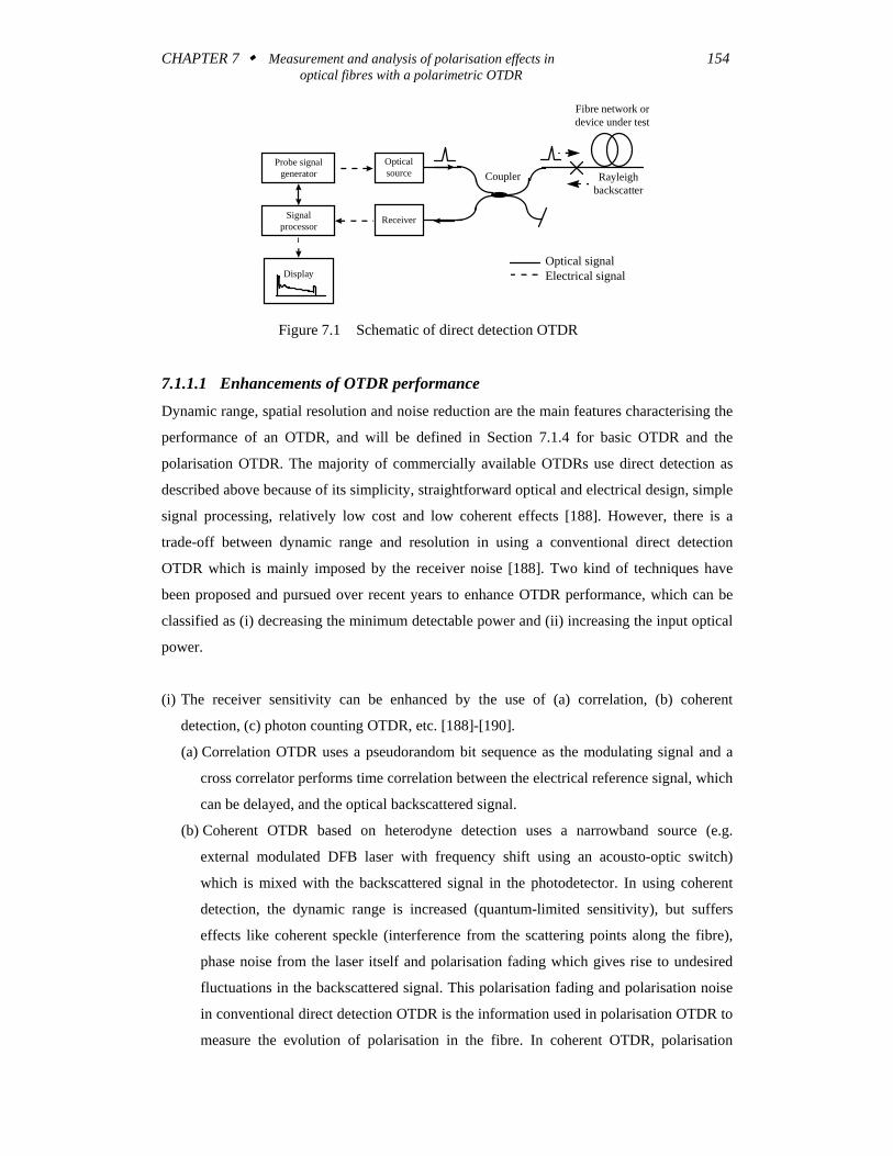
A general outline of a direct detection OTDR is shown in a schematic diagram in Figure 7.1.
A pulse from an laser source driven from an electrical pulse generator is launched over a
directional coupler into an optical fibre where the pulse undergoes Rayleigh scattering along
the fibre (Section 2.5). The backscattered power is then separated from the launched signal
via a directional coupler to an optical detector (usually APD) which converts the optical
signal to an electrical signal. The electrical signal is then amplified, digitised by an A/D
converter and averaged in the signal processing unit to improve the signal-to-noise ratio.
Finally, the backscattered signal is displayed as a function of time (distance) in logarithmic
form. The repetition rate of the pulse must be chosen such that the signals returning from the
fibre do not overlap. This is typically from 1 to 20 kHz depending on fibre length.
1 Commercial interest after publishing the work described in this chapter has been shown by various manufacturers of optical instruments.
CHAPTER 7 Measurement and analysis of polarisation effects in 154 optical fibres with a polarimetric OTDR
Optical signalElectrical signal
Opticalsource
Signalprocessor
Probe signalgenerator
Receiver
Fibre network ordevice under test
Coupler Rayleighbackscatter
Display
Figure 7.1 Schematic of direct detection OTDR
7.1.1.1 Enhancements of OTDR performance
Dynamic range, spatial resolution and noise reduction are the main features characterising the
performance of an OTDR, and will be defined in Section 7.1.4 for basic OTDR and the
polarisation OTDR. The majority of commercially available OTDRs use direct detection as
described above because of its simplicity, straightforward optical and electrical design, simple
signal processing, relatively low cost and low coherent effects [188]. However, there is a
trade-off between dynamic range and resolution in using a conventional direct detection
OTDR which is mainly imposed by the receiver noise [188]. Two kind of techniques have
been proposed and pursued over recent years to enhance OTDR performance, which can be
classified as (i) decreasing the minimum detectable power and (ii) increasing the input optical
power.
(i) The receiver sensitivity can be enhanced by the use of (a) correlation, (b) coherent
detection, (c) photon counting OTDR, etc. [188]-[190].
(a) Correlation OTDR uses a pseudorandom bit sequence as the modulating signal and a
cross correlator performs time correlation between the electrical reference signal, which
can be delayed, and the optical backscattered signal.
(b) Coherent OTDR based on heterodyne detection uses a narrowband source (e.g.
external modulated DFB laser with frequency shift using an acousto-optic switch)
which is mixed with the backscattered signal in the photodetector. In using coherent
detection, the dynamic range is increased (quantum-limited sensitivity), but suffers
effects like coherent speckle (interference from the scattering points along the fibre),
phase noise from the laser itself and polarisation fading which gives rise to undesired
fluctuations in the backscattered signal. This polarisation fading and polarisation noise
in conventional direct detection OTDR is the information used in polarisation OTDR to
measure the evolution of polarisation in the fibre. In coherent OTDR, polarisation
CHAPTER 7 Measurement and analysis of polarisation effects in 155 optical fibres with a polarimetric OTDR
fading and speckle fluctuation are reduced by employing polarisation and frequency
scrambling which adds further to the complexity of coherent OTDR.
(c) Photon counting OTDR showing centimetre resolution with high sensitivity, by using
pico second pulses in combination with a single-photon avalanche detector [189],
would be the optimum choice for a POTDR when measuring short lengths of fibre2.
However, the relatively long measurement time and very high purchase price are
drawbacks.
(ii) Enhancement of optical power can be achieved by using high power sources like a Q-
switched Er3+ glass laser at 1.55μm. Another very attractive method for increasing OTDR
performance is to employ erbium-doped fibre amplification of both the transmitted pulse
and the backscattered signal [191]-[193]. Optical amplification using a boost amplifier has
been used in the single-channel POTDR to enhance the output power of a conventional
direct detection OTDR. However, there is a non-linear power limitation in the maximum
probe pulse power due to non-linear scattering caused by stimulated Raman and Brillouin
scattering (Section 2.5). The critical peak power limit at λ = 1.55 μm using highly
coherent sources, has been given in [188] for Raman scattering as larger than +34 dBm
and for Brillouin scattering for pulsewidths < 1 μs as larger than +28 dBm3.
7.1.2 Enhanced OTDR using erbium doped fibre amplifiers Erbium doped fibre amplifiers give not only a significant advance in lightwave
communication systems but also in optical devices, as mentioned above for OTDR, to
increase the output power or minimum detectable power of the device. For the single-channel
polarisation OTDR such an enhanced high resolution large dynamic range OTDR was directly
available to us for the experiments [192]. The enhanced OTDR consists of a commercial
OTDR with boost amplifiers and control box with an optical switch to prevent amplified
spontaneous emission (ASE) from the erbium amplifiers entering the fibre when there is no
pulse.
2 A demonstration of a commercial photon counting OTDR with centimetre resolution working at 1.55μm from Opto-Electronics Inc., Canada modified to a POTDR (with fibre polariser) has been demonstrated at Essex University in May 96 (Purchase price ~ £90.000). 3 OTDR action: large repetition rates (~ 1 to ~20 kHz), average power is very low.
CHAPTER 7 Measurement and analysis of polarisation effects in 156 optical fibres with a polarimetric OTDR
7.1.2.1 Experimental OTDR set-up
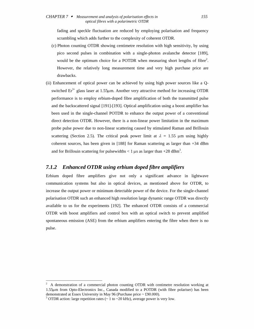
A block diagram of the enhanced OTDR set-up is shown in Figure 7.2. It consists of a
commercially available high resolution OTDR modified with a DFB laser and erbium
amplifiers to extend the dynamic range. The main frame (Anritsu OTDR MW 920A at 1.55
μm) drives the laser and performs the optical to electrical conversion with digital averaging of
the backscattered signal. The available pulsewidths are 6, 25 and 160 ns and the repetition
rate of 2.5 kHz and 1.25 kHz is set by the distance range (DR) of 15 km and 40 km
respectively. The external DFB laser has a centre wavelength at 1.55 μm with peak output
power of 0 dBm. The erbium-doped amplifiers, developed at BT Laboratories, are used as
power amplifiers to amplify the peak output power from the DFB laser from 0 dBm to +11
dBm with commensurate increase in the two way dynamic range. Optical isolators are used to
protect the DFB laser and to prevent lasing of the amplifiers from external reflections.
Isolator
PC
Optical signalElectrical signal
25 ns
DFB Laser1.55 μμm EDFAs A/O
Switch
APD receiverAmplifier section
A/D converterMicro-computer
Averaging processor
OTDR
Pulse generator
Timing anddriver circuitry
3 dBcoupler
Collimators used forPOTDR (~3 dB loss)
Isolator
Fibre under test
Figure 7.2 Block diagram of modified OTDR with DFB laser and erbium doped amplifiers.
The acousto-optical switch (AOS) works as a filter in the time domain, being synchronised to
open as the amplified pulse reaches the appropriate part of the transmitter, thus allowing only
the amplified pulse to pass and preventing receiver saturation from amplified spontaneous
emission (ASE) noise and pump laser power. The extinction ratio of the switch is larger then
35 dB. The optical pulse is then passed through a coupler (polarisation insensitive) separating
the transmit and receiver path. The backscattered light after passing the collimators (which
will be used for POTDR), is then detected by an avalanche photo diode within the main frame
of the OTDR. The bandwidth (BW) of the optical detector and amplifier section after the
optical detector is about 80 MHz. The backscattered signal is (after A/D conversion) averaged
in 501 buckets which are the sample points along the measured fibre length. The data can be
accessed using the OTDR GPIB interface and a computer to analyse the backscattered data.
CHAPTER 7 Measurement and analysis of polarisation effects in 157 optical fibres with a polarimetric OTDR
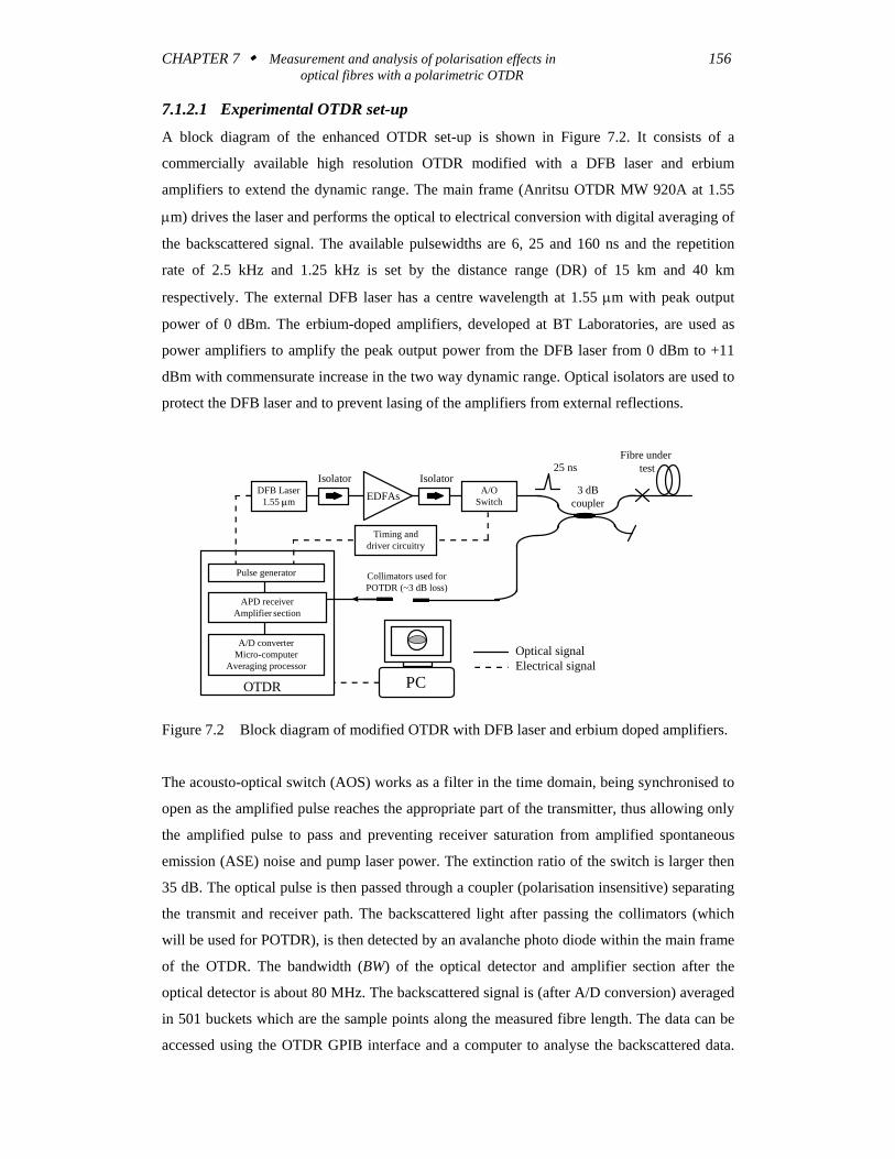
Figure 7.3(b) shows the measured OTDR trace on a ~1.7 km single mode fibre using the
enhanced OTDR as shown in Figure 7.2, with pulsewidth of 25 ns and no averaging. It can be
seen that the single way dynamic range is about 3.5 dB without any averaging. The one way
dynamic range is half the two way dynamic range if measured on the OTDR screen, because
the OTDR displays the one way fibre attenuation and a division by 2 is performed in the
vertical scale.
-100
-80
-60
-40
-20
0
Initial backscatter power level
Peak NEP
RMS NEP
Saturated response
Dead zone
DR without averaging
DR with averaging
Reflectione.g. connector
Splice
Bac
ksca
ttere
d po
wer
dB
m
Distance
-50
-40
-30
-20
-10
0
0 1 2 3 4 5Distance (km)
Bac
ksca
ttere
d po
wer
(dB
)
One way DR without averaging ~ 3.5 dB
A
B
A B
A: Fresnel reflection from fibre inputB: Fresnel reflection from end of fibre
(a) (b)
Figure 7.3 In (a) sketch of OTDR waveform with different losses and the effect of
averaging on the DR. In (b) trace of enhanced OTDR (with collimators in return
path) measured on ~1.7 km single mode fibre with 25 ns pulsewidth and without
averaging.
The external DFB laser in the OTDR set-up in Figure 7.2 has been used to obtain a well
polarised output SOP (DOP > 94% see Section 7.1.5) which is essential for POTDR. This was
necessary because using the internal Fabry-Perot laser (inside the OTDR) with its broad
spectrum4 required a fibre polariser to be inserted in the output path of the OTDR due to
depolarisation by the ‘poor’ isolators5 which had high PMD values. Using the fibre polariser
to polarise the depolarised pulse incurs an additional loss of about 4 dB (including insertion
loss). The majority of POTDR measurements have been performed by using the DFB laser. In
Appendix B, there is also a measurement shown by using a Fabry-Perot laser with fibre
polariser at the output.
The DFB lasers large coherence length is also of benefit if measuring long fibre lengths of
fibre because of its lower sensitivity to pulse broadening due to fibre dispersion compared
4 The envelope of the Fabry-Perot laser spectrum has been measured to have a 3 dB width of ~ 12 nm whereas for the DFB laser the 3 dB linewidth can be taken as less than 100 MHz. 5 These old isolators showed PMD values around 5 ps but were the only ones available to us at that time.
CHAPTER 7 Measurement and analysis of polarisation effects in 158 optical fibres with a polarimetric OTDR
with the Fabry-Perot laser. Furthermore, for POTDR applications, the pulse remains polarised
over greater lengths of the measured fibre.
7.1.3 Experimental polarimetric OTDR set-up Polarisation OTDR has been demonstrated in the laboratory with various configurations being
used to extract the polarisation information from the backscattered trace. A simple way of
extracting the polarisation information is by placing a polariser in the receiver path of the
OTDR, as for example, in [194]-[196]. The polarisation information in the backscattered
intensity can also be observed by simply placing a fibre polariser between the OTDR output
and the fibre under test where the polariser for the launched pulse acting as a polariser and for
the backscattered light as an analyser. However, by using just a polariser only one Stokes
component of the polarised light is obtained (Chapter 4), and in order to extract the full
information contained in the backscattered SOP, a general compensator analyser combination
has to be used as discussed in Chapter 4 for polarimetry. In [197], a polarimetric OTDR has
been demonstrated to obtain the full Stokes vector by using an electro-optic modulator and
rotating polaroid filter (sheet polariser) combination at λ ~ 0.5 μm.
Next, the modification of the enhanced OTDR in Figure 7.2 will be shown by simple
polarimetric means as discussed in Chapter 4. It should be noted that although optical
amplification is used to enhance the dynamic range in the relatively ‘old’ OTDR (made in
1990), the following method described could be directly used to extract the backscattered
SOP information in modern high resolution conventional OTDRs if they possess a single way
dynamic range of at least 10 dB.
7.1.3.1 The modification for analysing the backscattered SOP
The enhanced OTDR has been transformed to a polarimetric OTDR by using a computer
controlled λ/4 waveplate-linear polariser combination, placed between the two collimators in
the receiver path of the OTDR, Figure 7.4. The SOP from the backscattered intensity
containing the polarisation information, could be calculated by rotating the λ/4 plate to at
least four independent positions, for example, −30, 0°, 30° and 60°, as discussed in Section
4.2. In the following experiments, the λ/4 plate has been rotated to 19 analyser positions from
0° to 180°, and the backscattered SOP calculated from the measured intensities using a least
square identification [165]. This improved the calculated SOP considerably, compared to just
using four analyser positions, due to noise reduction in the individual Stokes components.
However, the measurement time increases and in fibres, where the SOP is not stable, for
example, aerial cables (ground wire of electricity pylons), it may be preferable to use no more
CHAPTER 7 Measurement and analysis of polarisation effects in 159 optical fibres with a polarimetric OTDR
than four analyser positions. Rotation of the polariser has been avoided because of the beam
deflection which would lead to an error in the analysed SOP (see Subsection 4.3.5). The
measurement time for one set of measurement results to obtain the backscattered SOP is about
30 minutes, which includes rotating of the λ/4 plate to 19 analyser positions, averaging and
data transfer to the computer.
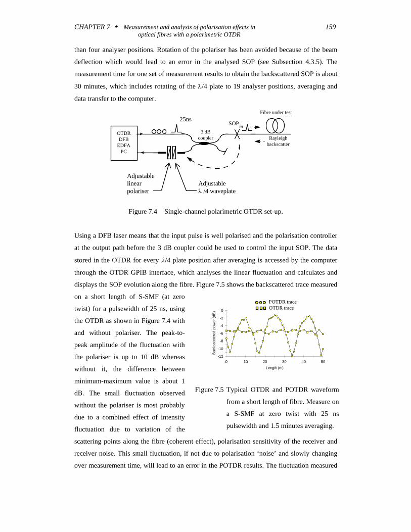
Adjustableλ /4 waveplate
Adjustablelinearpolariser
25nsSOP in
OTDRDFB
EDFAPC
3 dBcoupler
Fibre under test
Rayleighbackscatter
Figure 7.4 Single-channel polarimetric OTDR set-up.
Using a DFB laser means that the input pulse is well polarised and the polarisation controller
at the output path before the 3 dB coupler could be used to control the input SOP. The data
stored in the OTDR for every λ/4 plate position after averaging is accessed by the computer
through the OTDR GPIB interface, which analyses the linear fluctuation and calculates and
displays the SOP evolution along the fibre. Figure 7.5 shows the backscattered trace measured
on a short length of S-SMF (at zero
twist) for a pulsewidth of 25 ns, using
the OTDR as shown in Figure 7.4 with
and without polariser. The peak-to-
peak amplitude of the fluctuation with
the polariser is up to 10 dB whereas
without it, the difference between
minimum-maximum value is about 1
dB. The small fluctuation observed
without the polariser is most probably
due to a combined effect of intensity
fluctuation due to variation of the
scattering points along the fibre (coherent effect), polarisation sensitivity of the receiver and
receiver noise. This small fluctuation, if not due to polarisation ‘noise’ and slowly changing
over measurement time, will lead to an error in the POTDR results. The fluctuation measured
-12
-10
-8
-6
-4
-2
0
0 10 20 30 40 50Length (m)
Back
scat
tere
d po
wer
(dB)
POTDR traceOTDR trace
Figure 7.5 Typical OTDR and POTDR waveform
from a short length of fibre. Measure on
a S-SMF at zero twist with 25 ns
pulsewidth and 1.5 minutes averaging.
CHAPTER 7 Measurement and analysis of polarisation effects in 160 optical fibres with a polarimetric OTDR
with polariser (Figure 7.5) has been obtained by varying the input SOP and quarter
waveplate-polariser axis orientation to obtain maximum fluctuation.
7.1.3.2 Review of work on polarisation OTDR in the literature
Reported POTDR application and measurement results in the past may be grouped into (i)
theoretical work, (ii) sensor applications by analysing the backscatter in single mode fibres
and neglecting twist, (iii) measuring of linear birefringence, (iv) determination of mode
coupling in HiBi fibres and (v) estimation of PMD.
(i) A mainly theoretical treatment for analysing the birefringence from the backscattered light,
but assuming only linear birefringence, can also be found in [16], [198]-[200], where the
first three references also consider practical measurement limitations and factors affecting
the sensitivity and accuracy of POTDR.
(ii) The POTDR has been extensively treated for sensing applications such as electric and
magnetic fields and temperature monitoring [201]-[204], where its effectiveness in the
presence of magnetic fields has been demonstrated in [205].
(iii) The fibre birefringence along an optical fibre has been estimated from the backscattered
POTDR signal. In analysing the power spectrum from the POTDR fluctuation [195], one
sharp peak was observed and related to the polarisation beat length, but with no mention of
twist in the fibre. Reference [206] showed that by bending a fibre around a small diameter
drum without twisting, the linear birefringence due to bending (Subsection 3.3.7) can be
estimated from the POTDR fluctuation. In [197], a polarimetric OTDR at λ ~ 0.5 μm has
been used to obtain the full Stokes vector and to estimate the linear birefringence in the
fibre. It was mentioned that circular birefringence (which cannot be totally avoided) could
influence the measurement results but the effect of twist on POTDR signal was not
considered any further. In [207], an interesting method of downshifting the measured
POTDR fluctuation by optical beating of the backscattered signal from two lasers was
demonstrated, reducing the minimum measurable fluctuation due to the receiver
bandwidth.
(iv) Mode coupling along high birefringence fibres has been analysed [208] and measured
using POTDR [209], [210]. The input SOP has been aligned with one of the principal axes
of the fibre and the backscattered light has been analysed through a rotatable polariser at
0° and 90° to the principle axes of the HiBi fibre.
(v) Detection of sections with large PMD by using POTDR with a single polariser in the
receiver path. The methods include counting the periodicity in the POTDR fluctuation
[196], observing the power spectrum from the fluctuation [211], [212], and trying to
CHAPTER 7 Measurement and analysis of polarisation effects in 161 optical fibres with a polarimetric OTDR
identify from the magnitude of the POTDR fluctuation, fibre sections where the launched
pulse is strongly depolarised, which would correspond to a high PMD [213]. In the
references [196], [211]-[213], the fibre is assumed to possess only linear birefringence.
In the above literature, it has often been assumed that a fibre may be described as a system of
linear retarder-rotator combinations, and for the light travelling in reverse direction, the
rotator is reversed and is cancelled. However, this assumption is not valid for twisted fibres
because although the circular birefringence induced by twist cancels for the combined
forward-backward transmission (see Section 6.2), there is also a geometrical rotation of the
local linear birefringence. It will be shown from Section 7.2 onwards, theoretically and by
measurement, that even a small amount of twist can have a large influence on the POTDR
fluctuation, and if neglected, leads to a large error in the estimated birefringence and DGD
[15] [170] [214] [215].
7.1.4 Performance parameters of the POTDR This section treats at first the backscattered optical power from a single mode fibre. From that,
the main performance parameters for OTDR and POTDR will be discussed and given for the
single-channel polarimetric OTDR. The parameters considered are the dynamic range, the
spatial resolution and a more POTDR specific parameter, the DOP of the launched pulse and
its repeatability with time. These performance parameters will determine the error in the
measured backscattered SOP and the POTDR waveform periodicity and will be reconsidered
at the beginning of Section 7.3 which treats the measurement results.
7.1.4.1 Backscattered mean power
The Rayleigh backscattered power PR in a step index fibre from a rectangular optical pulse
with a width W and peak power P0, observed at the input end of the fibre at the time t is [216]
( )P l S Wv PR s g
v tg=
−12
10010αα
(7.1)
where S is the backscattering capture coefficient, αS the loss coefficient due to Rayleigh
scattering which is about 0.18 dB/km for pure silica (Equation 2.24), but depends also on the
doping level, W is the pulsewidth, α is the fibre loss coefficient which is about 0.2 to 0.25
dB/km at λ = 1.55 μm in single mode fibres and vg the group velocity. The group velocity in a
fibre is defined by Equation 3.10 as vg = c/ng and for simplicity, we may assume ng is
CHAPTER 7 Measurement and analysis of polarisation effects in 162 optical fibres with a polarimetric OTDR
constant, so that c/n represents approximately the light velocity in the fibre and the time t
corresponds to the position l ≈ ct/(2n) in the fibre, with 2αl the round trip loss.
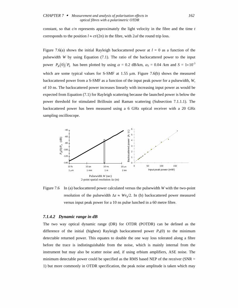
Figure 7.6(a) shows the initial Rayleigh backscattered power at l = 0 as a function of the
pulsewidth W by using Equation (7.1). The ratio of the backscattered power to the input
power ( )P PR 0 0 has been plotted by using α = 0.2 dB/km, αS = 0.04 /km and S = 1×10⁻³
which are some typical values for S-SMF at 1.55 μm. Figure 7.6(b) shows the measured
backscattered power from a S-SMF as a function of the input peak power for a pulsewidth, W,
of 10 ns. The backscattered power increases linearly with increasing input power as would be
expected from Equation (7.1) for Rayleigh scattering because the launched power is below the
power threshold for stimulated Brillouin and Raman scattering (Subsection 7.1.1.1). The
backscattered power has been measured using a 6 GHz optical receiver with a 20 GHz
sampling oscilloscope.
0
1
2
3
4
5
6
0 50 100 150
Input peak power (mW)
Bac
ksca
ttere
d po
wer
(A
. U.)
P R(0
)/P0
(dB
)
-140
-120
-100
-80
-60
-40
10 μs
Pulsewidth W (sec)2-point spatial resolution Δz (m)
10 ns10 ps10 fs
1 km1 m1 mm1 μm
Figure 7.6 In (a) backscattered power calculated versus the pulsewidth W with the two-point
resolution of the pulsewidth Δz ≈ Wvg/2. In (b) backscattered power measured
versus input peak power for a 10 ns pulse lunched in a 60 metre fibre.
7.1.4.2 Dynamic range in dB
The two way optical dynamic range (DR) for OTDR (POTDR) can be defined as the
difference of the initial (highest) Rayleigh backscattered power P0(0) to the minimum
detectable returned power. This equates to double the one way loss tolerated along a fibre
before the trace is indistinguishable from the noise, which is mainly internal from the
instrument but may also be scatter noise and, if using erbium amplifiers, ASE noise. The
minimum detectable power could be specified as the RMS based NEP of the receiver (SNR =
1) but more commonly in OTDR specification, the peak noise amplitude is taken which may
CHAPTER 7 Measurement and analysis of polarisation effects in 163 optical fibres with a polarimetric OTDR
be taken as about 3 times larger than the RMS value (3σ for Gaussian noise with zero mean).
The two way DR can be expressed as
( ) ( ) ( ) ( ) ( )DR dBP
NEPP dBm NEP dBmR
PeakR Peak=
⎛
⎝⎜
⎞
⎠⎟ = −10
00log (7.2)
The one way DR including the factor 2 for round trip loss is half the DR specified in Equation
(7.2) and can be directly obtained from the OTDR display as indicated in Figure 7.3 (a) and
(b), which automatically includes all the noise contributions and also the loss due to the
coupler. For POTDR applications with an analyser in the receiver path and short fibre lengths
(< 1 km), so that the fibre loss can be neglected, the two way dynamic range is important and
will determine the noise error in the measured SOP (Section 4.4).
Averaging of the backscattered signal after repetitively measuring over many pulses improves
the SNR. The arithmetic average of the samples can be generated by using an analogue
method (boxcar averaging), or by digital averaging after the A/D conversion is performed
(Figure 7.2). Assuming Gaussian distributed noise, the reduction in NEP is proportional to the
inverse square root of the number, N, of measurements [188]
NEP NEP NAv = (7.3)
For a 20 dB noise suppression, a time averaging of 104 values would be needed (Equation
(7.3)), but in practice the improvement in the SNR will saturate through effects like the
quantization noise from the A/D converter if using digital averaging, and also drift in the
receiver.
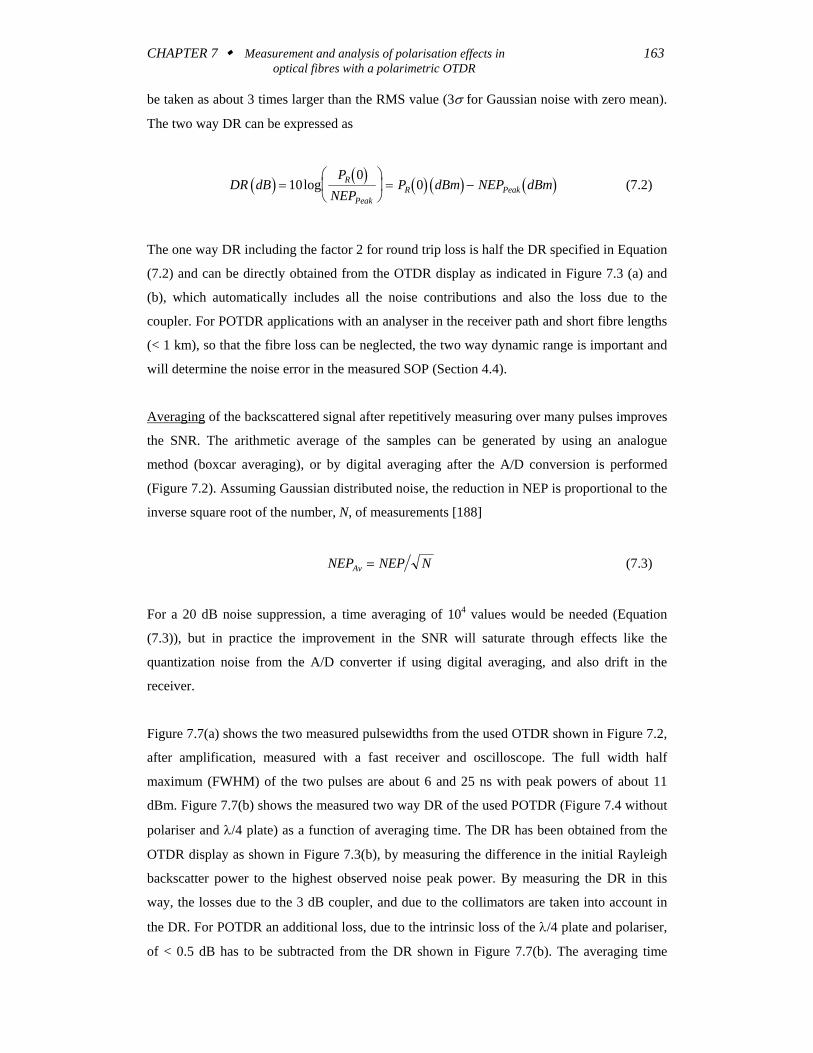
Figure 7.7(a) shows the two measured pulsewidths from the used OTDR shown in Figure 7.2,
after amplification, measured with a fast receiver and oscilloscope. The full width half
maximum (FWHM) of the two pulses are about 6 and 25 ns with peak powers of about 11
dBm. Figure 7.7(b) shows the measured two way DR of the used POTDR (Figure 7.4 without
polariser and λ/4 plate) as a function of averaging time. The DR has been obtained from the
OTDR display as shown in Figure 7.3(b), by measuring the difference in the initial Rayleigh
backscatter power to the highest observed noise peak power. By measuring the DR in this
way, the losses due to the 3 dB coupler, and due to the collimators are taken into account in
the DR. For POTDR an additional loss, due to the intrinsic loss of the λ/4 plate and polariser,
of < 0.5 dB has to be subtracted from the DR shown in Figure 7.7(b). The averaging time
CHAPTER 7 Measurement and analysis of polarisation effects in 164 optical fibres with a polarimetric OTDR
used in the backscattered SOP measurements (Section 7.3) is 1.5 minutes in order to keep
measurement time reasonable and still have a reasonable noise reduction. For 1.5 minutes
averaging time, the DR for the 25 ns pulse is about 21 dB and about 9 dB for the 6 ns pulse.
In Section 4.4, it has been shown that in order to keep the error reasonable in the measured
SOP, the SNR should be above 10 dB (Figure 4.9, ε < 20°) which is why for the single-
channel POTDR the 6 ns pulse was not used, although it would give a higher resolution.
0
5
10
15
20
25
0 60 120 180 240 300 360Averaging time (sec)
DR
(dB
)
Measurementaveraging time
0
4
8
12
16
0 10 20 30 40 50Time (ns)
Pow
er (m
W)
PW: 25 ns
PW: 6 ns
(a) (b)
Figure 7.7 DR increase with averaging In (b) for 25 ns pulse two way DR ~ 20 dB for 90
second averaging.
7.1.4.3 Principle error sources
The absolute distance resolution which may be calculated from l ≈ ct/(2n) depends on the
fibre refractive index which may change slightly from fibre to fibre, and further depends on
the accuracy and stability of the instrument time base (sampling resolution). For short
distances, the error in the time base will be dominant, whereas for long distances, it is the
error in the refractive index. However, for the reported POTDR measurements, we are only
interested in short distances and the relative difference between measurement points is of
more importance and will be treated in Subsection 7.1.4.4.
The accuracy and linearity of the vertical scale depends not only on internal parameters of the
OTDR, such as the linearity of the amplifiers and the quantization noise induced by the A/D
converter, but also on the SNR and noise in the scattered intensity, such as polarisation and
coherent scatter noise. For POTDR, the dominant error source in the vertical scale is the
limited SNR as shown in Figure 7.7(b), and also some small fluctuation as observed in the
measured OTDR intensity in Figure 7.5 which is not due to just polarisation noise.
7.1.4.4 Two-point resolution in metres
The two-point resolution (spatial resolution) is a measure of the closest spacing between two
fibre discontinuities which the OTDR (POTDR) can separate. Assuming sufficient SNR to
CHAPTER 7 Measurement and analysis of polarisation effects in 165 optical fibres with a polarimetric OTDR
separate the signal from the noise, the two-point resolution, Δz, is dependent upon the
pulsewidth W, and impulse receiver response time tr, and is calculated from [188]
Δzv
W tgr≈ +
22 2 (7.4)
The receiver response time may be taken as equal to the inverse of the detector bandwidth
BW, tr = 1/BW. Ideally, Δz should be small (short pulsewidth and large receiver bandwidth)
but as can now be seen, in comparing Equation (7.4) with Equation (7.1), there is a trade-off
between the two-point resolution and the SNR. For the used OTDR, the 3 dB cut-off
frequency is about 80 MHz which for the 25 and 6 ns pulse gives an estimated two-point
resolution from Equation (7.4) of about 2.8 and 1.4 metres respectively. For the calculation of
the two-point resolution in the fibre, a rectangular pulse is assumed and fibre dispersion
contribution to the pulsewidth has been neglected which is valid for short fibre lengths.
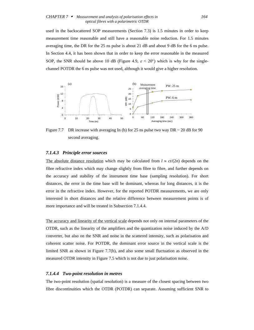
A direct measurement of Δz may be obtained from the OTDR display by measuring the
FWHM value of the pulse response from one reflection point in the fibre which in the
logarithmic scale is −3 dB from the maximum measured backreflected power. Figure 7.8 (a)
and (b) show the measured reflection from a fibre back to back connection measured with the
enhanced OTDR for the 25 and 6 ns pulsewidth respectively. Saturation has been avoided and
the − 3 dB points are about 2.5 and 1.2 metre for the 25 and 6 ns pulsewidth respectively,
which is only slightly less then expected from the theoretically estimated values above.
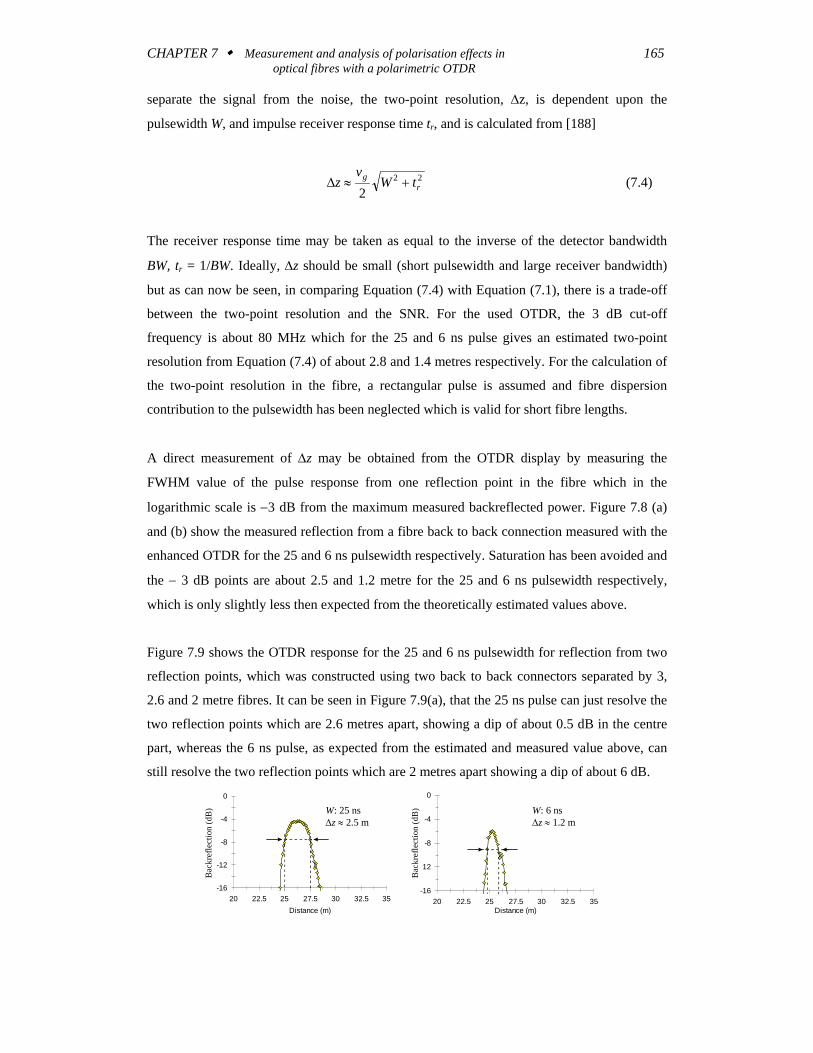
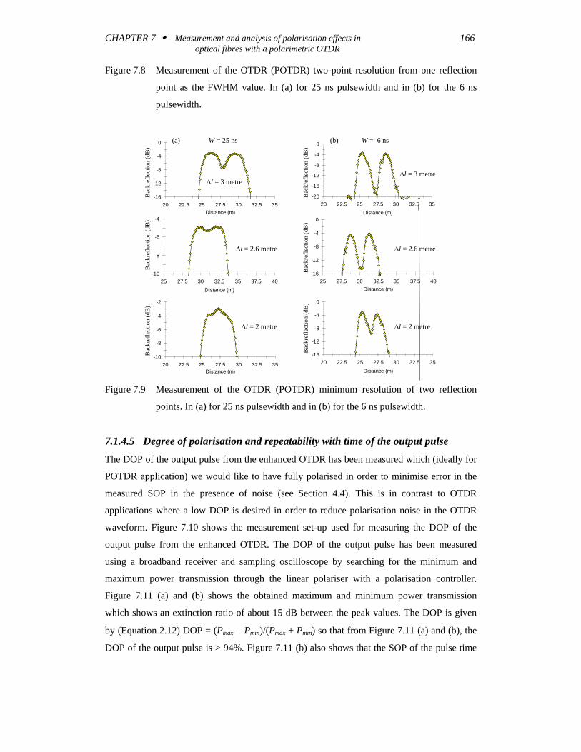
Figure 7.9 shows the OTDR response for the 25 and 6 ns pulsewidth for reflection from two
reflection points, which was constructed using two back to back connectors separated by 3,
2.6 and 2 metre fibres. It can be seen in Figure 7.9(a), that the 25 ns pulse can just resolve the
two reflection points which are 2.6 metres apart, showing a dip of about 0.5 dB in the centre
part, whereas the 6 ns pulse, as expected from the estimated and measured value above, can
still resolve the two reflection points which are 2 metres apart showing a dip of about 6 dB.
-16
-12
-8
-4
0
20 22.5 25 27.5 30 32.5 35Distance (m)
Bac
kref
lect
ion
(dB
)
-16
-12
-8
-4
0
20 22.5 25 27.5 30 32.5 35Distance (m)
Bac
kref
lect
ion
(dB
)W: 25 nsΔz ≈ 2.5 m
W: 6 nsΔz ≈ 1.2 m
Bac
kref
lect
ion
(dB
)
Bac
kref
lect
ion
(dB
)
CHAPTER 7 Measurement and analysis of polarisation effects in 166 optical fibres with a polarimetric OTDR
Figure 7.8 Measurement of the OTDR (POTDR) two-point resolution from one reflection
point as the FWHM value. In (a) for 25 ns pulsewidth and in (b) for the 6 ns
pulsewidth.
-16
-12
-8
-4
0
20 22.5 25 27.5 30 32.5 35Distance (m)
Back
refle
ctio
n (d
B)
-20
-16
-12
-8
-4
0
20 22.5 25 27.5 30 32.5 35Distance (m)
Back
refle
ctio
n (d
B)
-16
-12
-8
-4
0
20 22.5 25 27.5 30 32.5 35Distance (m)
Back
refle
ctio
n (d
B)
-10
-8
-6
-4
-2
20 22.5 25 27.5 30 32.5 35Distance (m)
Back
refle
ctio
n (d
B)
-16
-12
-8
-4
0
25 27.5 30 32.5 35 37.5 40Distance (m)
Back
refle
ctio
n (d
B)
-10
-8
-6
-4
25 27.5 30 32.5 35 37.5 40Distance (m)
Back
refle
ctio
n (d
B)(a) W = 25 ns (b) W = 6 ns
Δl = 3 metreΔl = 3 metre
Δl = 2 metre Δl = 2 metre
Δl = 2.6 metre Δl = 2.6 metre
Bac
kref
lect
ion
(dB)
Bac
kref
lect
ion
(dB
)B
ackr
efle
ctio
n (d
B)
Bac
kref
lect
ion
(dB)
Bac
kref
lect
ion
(dB
)B
ackr
efle
ctio
n (d
B)
Figure 7.9 Measurement of the OTDR (POTDR) minimum resolution of two reflection
points. In (a) for 25 ns pulsewidth and in (b) for the 6 ns pulsewidth.
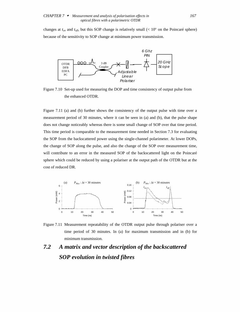
7.1.4.5 Degree of polarisation and repeatability with time of the output pulse
The DOP of the output pulse from the enhanced OTDR has been measured which (ideally for
POTDR application) we would like to have fully polarised in order to minimise error in the
measured SOP in the presence of noise (see Section 4.4). This is in contrast to OTDR
applications where a low DOP is desired in order to reduce polarisation noise in the OTDR
waveform. Figure 7.10 shows the measurement set-up used for measuring the DOP of the
output pulse from the enhanced OTDR. The DOP of the output pulse has been measured
using a broadband receiver and sampling oscilloscope by searching for the minimum and
maximum power transmission through the linear polariser with a polarisation controller.
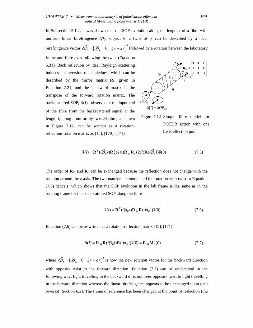
Figure 7.11 (a) and (b) shows the obtained maximum and minimum power transmission
which shows an extinction ratio of about 15 dB between the peak values. The DOP is given
by (Equation 2.12) DOP = (Pmax − Pmin)/(Pmax + Pmin) so that from Figure 7.11 (a) and (b), the
DOP of the output pulse is > 94%. Figure 7.11 (b) also shows that the SOP of the pulse time
CHAPTER 7 Measurement and analysis of polarisation effects in 167 optical fibres with a polarimetric OTDR
changes at ton and toff, but this SOP change is relatively small (< 10° on the Poincaré sphere)
because of the sensitivity to SOP change at minimum power transmission.
OTDRDFB
EDFAPC
20 GHzScope
AdjustableLinear
Polariser
6 GhzPIN
3 dBCoupler
Figure 7.10 Set-up used for measuring the DOP and time consistency of output pulse from
the enhanced OTDR.
Figure 7.11 (a) and (b) further shows the consistency of the output pulse with time over a
measurement period of 30 minutes, where it can be seen in (a) and (b), that the pulse shape
does not change noticeably whereas there is some small change of SOP over that time period.
This time period is comparable to the measurement time needed in Section 7.3 for evaluating
the SOP from the backscattered power using the single-channel polarimeter. At lower DOPs,
the change of SOP along the pulse, and also the change of the SOP over measurement time,
will contribute to an error in the measured SOP of the backscattered light on the Poincaré
sphere which could be reduced by using a polariser at the output path of the OTDR but at the
cost of reduced DR.
0
2
4
6
0 10 20 30 40 50Time (ns)
Pow
er (m
W)
0
0.04
0.08
0.12
0.16
0 10 20 30 40 50Time (ns)
Pow
er (m
W)
PMax : Δt = 30 minutes PMin : Δt = 30 minutes(a) (b)ton toff
Figure 7.11 Measurement repeatability of the OTDR output pulse through polariser over a
time period of 30 minutes. In (a) for maximum transmission and in (b) for
minimum transmission.
7.2 A matrix and vector description of the backscattered
SOP evolution in twisted fibres

CHAPTER 7 Measurement and analysis of polarisation effects in 168 optical fibres with a polarimetric OTDR
In this section, the matrix description for the backscattered SOP evolution in twisted fibres
will be derived, where the assumption made for the matrix description in forward direction
(Subsection 5.1.1) will be assumed to be also true for counter propagating waves.
In single mode fibres, we assume negligible dichroism (no PDL) for the forward direction,
uniform polarisation over the spatial mode field [55] and preservation of polarisation
orthogonality at all points along the fibre[42]. In Section 4.5, it has been shown that the fibre
behaves like a reciprocal medium and the assumptions for forward propagating waves can be
taken as valid for counterpropagating waves. This we would also expect from theory, so long
as the system behaves like a linear system (no Brillouin or Raman scattering), and in the
absence of any nonreciprocal effects (Section 2.4) like the Faraday effect.
A more severe assumption is concerned with the scattering process in the fibre itself where
ideal scattering in the derived model will be assumed. Ideal scattering, in this sense, we define
as scattering from a short pulse so that the SOP does not change significantly within the
pulsewidth (Section 7.5), so that there is no interference from the scattering points along the
fibre. Further the scatter points in the fibre are ideal isotropic scatterers (Subsection 2.5.3) so
that the scatter centre preserves the SOP (no phase or amplitude change). Under these
assumptions the scattering process can be described by a reflection from an ideal mirror
(Section 4.5) in describing the backscattered SOP evolution in an optical fibre.
The last assumption will be reconsidered in Section 7.5 because the measurement results
obtained with POTDR showed that the measured fibres did not behave as we would expect
from an ideal rotation matrix with ideal reflection which would preserve the DOP.
For ideal scattering and a linear reciprocal system, the magnitude of the Stokes vector is
constrained to unity length, and the backscatter matrix in a fibre with uniform linear and
circular birefringence can be obtained by extending the derived solution in Chapter 5 by
including the reflection matrix RM which changes the handedness of the scattered SOP.
7.2.1 A Mueller matrix description for backscattered light along
fibres with and without twist
CHAPTER 7 Measurement and analysis of polarisation effects in 169 optical fibres with a polarimetric OTDR
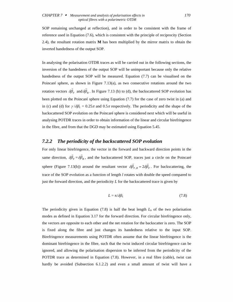
In Subsection 5.1.2, it was shown that the SOP evolution along the length l of a fibre with
uniform linear birefringence δβL, subject to a twist of γ, can be described by a local
birefringence vector ( )δβ δβ γ γr
F LT
g= −0 2 followed by a rotation between the laboratory
frame and fibre axes following the twist (Equation
5.31). Back reflection by ideal Rayleigh scattering
induces an inversion of handedness which can be
described by the mirror matrix RM given in
Equation 2.21, and the backward matrix is the
transpose of the forward rotation matrix. The
backscattered SOP, ss( )l , observed at the input end
of the fibre from the backscattered signal at the
length l, along a uniformly twisted fibre, as shown
in Figure 7.12, can be written as a rotation-
reflection-rotation matrix as [15], [170], [171]
s r r rs R R R R R s( ) ( ) ( ) ( ) ( ) ( )l l l l lTF z
TM z F= δβ γ γ δβ2 2 0 (7.5)
The order of RM and Rz can be exchanged because the reflection does not change with the
rotation around the z-axis. The two matrices commute and the rotation with twist in Equation
(7.5) cancels, which shows that the SOP evolution in the lab frame is the same as in the
rotating frame for the backscattered SOP along the fibre
s r r rs R R R s( ) ( ) ( ) ( )l l lTF M F= δβ δβ 0 (7.6)
Equation (7.6) can be re-written as a rotation-reflection matrix [15], [171]
s s r r rs R R R s R Ms( ) ( ) ( ) ( ) ( )l l lM B F M= =δβ δβ 0 0 (7.7)
where ( )δβ δβ γ γs
B LTg= −0 2 is now the new rotation vector for the backward direction
with opposite twist to the forward direction. Equation (7.7) can be understood in the
following way: light travelling in the backward direction sees opposite twist to light travelling
in the forward direction whereas the linear birefringence appears to be unchanged upon path
reversal (Section 6.2). The frame of reference has been changed at the point of reflection (the
R
RT
RM =1 0 00 1 00 0 - 1
SOPin
l
( )ss l SOPout= Figure 7.12 Simple fibre model for
POTDR action with one
backreflection point
CHAPTER 7 Measurement and analysis of polarisation effects in 170 optical fibres with a polarimetric OTDR
SOP remaining unchanged at reflection), and in order to be consistent with the frame of
reference used in Equation (7.6), which is consistent with the principle of reciprocity (Section
2.4), the resultant rotation matrix M has been multiplied by the mirror matrix to obtain the
inverted handedness of the output SOP.
In analysing the polarisation OTDR traces as will be carried out in the following sections, the
inversion of the handedness of the output SOP will be unimportant because only the relative
handedness of the output SOP will be measured. Equation (7.7) can be visualised on the
Poincaré sphere, as shown in Figure 7.13(a), as two consecutive rotations around the two
rotation vectors δβr
F andδβs
B . In Figure 7.13 (b) to (d), the backscattered SOP evolution has
been plotted on the Poincaré sphere using Equation (7.7) for the case of zero twist in (a) and
in (c) and (d) for γ /δβL = 0.25π and 0.5π respectively. The periodicity and the shape of the
backscattered SOP evolution on the Poincaré sphere is considered next which will be useful in
analysing POTDR traces in order to obtain information of the linear and circular birefringence
in the fibre, and from that the DGD may be estimated using Equation 5.45.
7.2.2 The periodicity of the backscattered SOP evolution For only linear birefringence, the vector in the forward and backward direction points in the
same direction, δβr
F =δβs
B , and the backscattered SOP, traces just a circle on the Poincaré
sphere (Figure 7.13(b)) around the resultant vector δβ δβr r
F B F, = 2 . For backscattering, the
trace of the SOP evolution as a function of length l rotates with double the speed compared to
just the forward direction, and the periodicity L for the backscattered trace is given by
L = π/δβL (7.8)
The periodicity given in Equation (7.8) is half the beat length Lb of the two polarisation
modes as defined in Equation 3.17 for the forward direction. For circular birefringence only,
the vectors are opposite to each other and the net rotation for the backscatter is zero. The SOP
is fixed along the fibre and just changes its handedness relative to the input SOP.
Birefringence measurements using POTDR often assume that the linear birefringence is the
dominant birefringence in the fibre, such that the twist induced circular birefringence can be
ignored, and allowing the polarisation dispersion to be inferred from the periodicity of the
POTDR trace as determined in Equation (7.8). However, in a real fibre (cable), twist can
hardly be avoided (Subsection 6.1.2.2) and even a small amount of twist will have a
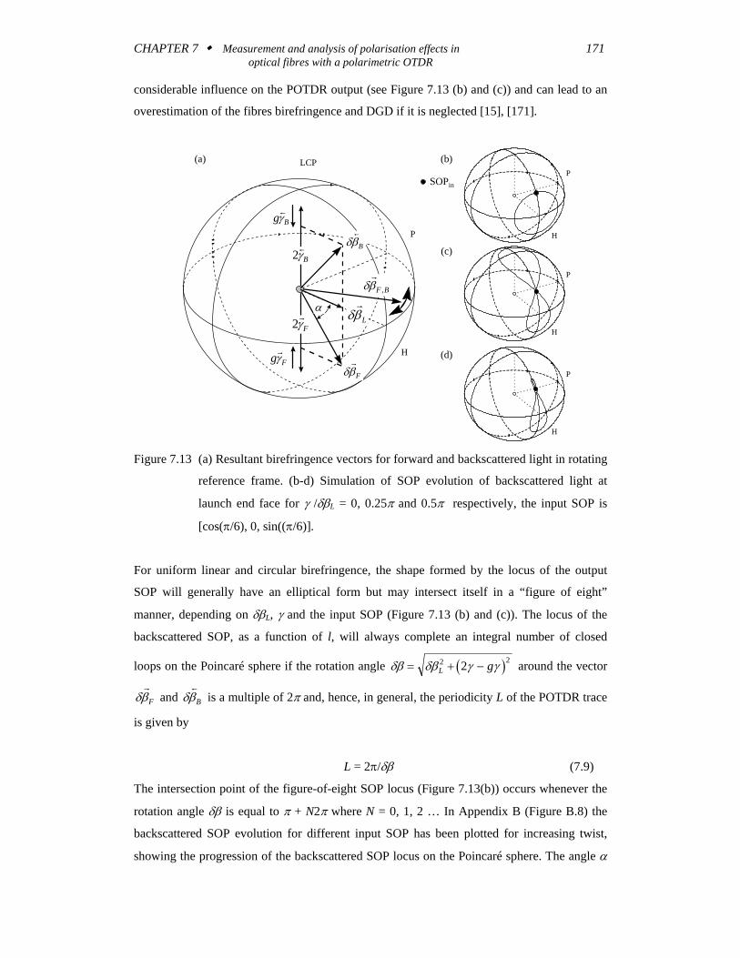
CHAPTER 7 Measurement and analysis of polarisation effects in 171 optical fibres with a polarimetric OTDR
considerable influence on the POTDR output (see Figure 7.13 (b) and (c)) and can lead to an
overestimation of the fibres birefringence and DGD if it is neglected [15], [171].
(a)
H
P
LCP
δβr
L2rγF
2sγB
g Bsγ
g Frγ
δβr
F B,
δβr
F
δβs
B
α
SOPin
H
P
H
P
H
P
(b)
(c)
(d)
Figure 7.13 (a) Resultant birefringence vectors for forward and backscattered light in rotating
reference frame. (b-d) Simulation of SOP evolution of backscattered light at
launch end face for γ /δβL = 0, 0.25π and 0.5π respectively, the input SOP is
[cos(π/6), 0, sin((π/6)].
For uniform linear and circular birefringence, the shape formed by the locus of the output
SOP will generally have an elliptical form but may intersect itself in a “figure of eight”
manner, depending on δβL, γ and the input SOP (Figure 7.13 (b) and (c)). The locus of the
backscattered SOP, as a function of l, will always complete an integral number of closed
loops on the Poincaré sphere if the rotation angle ( )δβ δβ γ γ= + −L g2 22 around the vector
δβr
F and δβs
B is a multiple of 2π and, hence, in general, the periodicity L of the POTDR trace
is given by
L = 2π/δβ (7.9)
The intersection point of the figure-of-eight SOP locus (Figure 7.13(b)) occurs whenever the
rotation angle δβ is equal to π + N2π where N = 0, 1, 2 … In Appendix B (Figure B.8) the
backscattered SOP evolution for different input SOP has been plotted for increasing twist,
showing the progression of the backscattered SOP locus on the Poincaré sphere. The angle α
CHAPTER 7 Measurement and analysis of polarisation effects in 172 optical fibres with a polarimetric OTDR
between the resultant vector δβr
F and the equatorial plane (or δβs
B ) as indicated in Figure
7.13(a), determines (for a fixed input SOP) the shape of the SOP evolution on the Poincaré
sphere and is given by
( ) ( )tan αγ γδβ
=−2 g
L
(7.10)
From Equation (7.9) and (7.10), it may be seen that if the periodicity L and angle α of the
resultant vector in forward or backward direction are known (or in other words the shape of
the SOP evolution on the Poincaré sphere), then the magnitude of the linear birefringence and
the twist of a fibre may be estimated from the backscattered SOP evolution using POTDR.
7.2.3 The response of an analyser The dual occurrence of the rotation matrix R in Equation (7.7) indicates that the matrix
coefficients of M are quadratic in cos(δβ•l) and sin(δβ•l) (see Equation 5.30), and in general,
the intensity through an analyser (Section 4.2) may be expressed in the form of a Fourier
series [15]
( ) ( )
( ) ( )
I a a n l b n l
a a l b l
n nn
n n n nn
= + +
= + +
=
=
∑
∑
01
2
01
2
2 2
cos sin
cos sin
δβ δβ
πκ πκ (7.11)
where the magnitudes of the coefficients a and b depends on the linear and circular
birefringence, and the input SOP and κ1,2 are the spatial frequencies in cycles/m. For the
simple case of zero twist, the SOP traces just a circle (Figure 7.13(b)) as discussed above, a1
and b1 being zero, leading to just one component in the POTDR power spectrum, as expected
from Equation (7.8). For backreflection from a section with twist, a1 and b1 are now not zero
which, together with a2 and b2, lead to two components in the POTDR spectrum, which may
be called the fundamental and second harmonic fluctuations. This qualitative difference
between the two POTDR spectra makes it, in general, possible to detect sections of fibre with
twist and no twist for an arbitrary input SOP and fixed analyser position, as will be shown in
Section 7.3, where the limitations in analysing POTDR output data using this method will
also be discussed.
CHAPTER 7 Measurement and analysis of polarisation effects in 173 optical fibres with a polarimetric OTDR
7.2.4 A vector description for backscattered light along fibres
with and without twist
In Figure 7.13(a), the rotation around the two vectors, δβr
F and δβs
B , can be replaced by a
single equivalent rotation [217] around the vector δβr
F B, given by [171]
( ) ( ) ( )( )tan $ tan
$ $ tan $ $
tan $ $, ,δβ δβ δβδβ δβ δβ δβ δβ
δβ δβ δβF B F BF B B F
F B
ll
l2 2
21 22=
+ + ×
− (7.12)
with the rotation angle δβF,B as ( )( )
tantan
tan,δβ
δβδβ
δβ
δβ γ δβδβ
δβF B
L
L C
b l
l
22
2
12
2
2 2
22
=
⎛⎝⎜
⎞⎠⎟
−− − ⎛
⎝⎜⎞⎠⎟
and the
rotation axis δβ δβ γδβ
δβ$ tan,F BC
bl= − ⎛
⎝⎜⎞⎠⎟
⎡
⎣
⎢⎢⎢⎢
⎤
⎦
⎥⎥⎥⎥
11
22
0
where ( )
bl C
= +
⎛⎝⎜
⎞⎠⎟
−1 2
22 2
2
tan δβ γ δβ
δβ.
Equation (7.12) gives a very useful form for implementation in a computing algorithm to
analyse the backscatter traces of POTDR, as will be used in Section 7.3 and 7.4. The rotation
axis of the resultant rotation in Equation (7.12) lies in the equatorial plane (see also Figure
7.13(a)), proving that for a reciprocal system in the presence of twist, the eigenvectors for one
round trip are linearly polarised, as shown in Section 4.5 for different optical elements.
However, although the circular birefringence cancels for one round trip and the fibre may
look, with respect to one backreflection point, as if it possesed just linear birefringence, the
presence of twist can still be observed with respect to a second backreflection point because
the direction and angle of rotation of δβr
F B, depends on the fibre twist. This would also be
expected because twist not only induces circular birefringence, but also reduces the effective
linear birefringence as shown in Figure 5.9. POTDR fluctuation is, in general, strongly
influenced by twist, as will be shown, but to differentiate between the two kinds of twist, i.e.
whether elastic twist or frozen in twist as in spun fibres, would be difficult from the POTDR
trace without prior knowledge of the kind of twist expected, due to the small effect of the
rotation coefficient (gγ compared to 2γ, g ≈ 0.14) in the resultant birefringence vector δβ in
Equation (7.12).
CHAPTER 7 Measurement and analysis of polarisation effects in 174 optical fibres with a polarimetric OTDR
7.3 Measurement results and analysis from the single-
channel POTDR on fibres with different twist rates
In this section, the POTDR measurement results on fibres with and without twist are shown.
The majority of the early results have been taken using the single-channel POTDR with DFB
laser which showed the type of results predicted from theory. Since the first reported results,
improvement of the measurement set-up, by using a fibre polariser at the output of the single-
channel polarimeter, and also by using a novel four-channel POTDR, has been obtained
reducing the error in the measured SOP (Section 7.4 and Appendix B, Figure B.6).
In the presence of twist the backscattered SOP evolution can be characterised by the
periodicity of the SOP evolution (Equation (7.9)) and by the shape of the SOP evolution if
plotted on the Poincaré sphere (Equation (7.10)). For the single-channel POTDR, the error in
the periodicity of the SOP evolution is determined by the two-point resolution, which is ~±3
metres (Subsection 7.1.4.4), and the error in the shape of the SOP evolution, which will be
treated in Section 7.5, may be taken as ±3.6° in the average overall SOP. For zero twist, the
error of ±3 metres, due to the two-point resolution, is determined by the periodicity of the
SOP evolution as given in Equation (7.8).
7.3.1 Measurement conditions
The experimental results using POTDR were carried out on some of the freely suspended
fibres described in Chapter 6 for measuring the DGD. Measuring the DGD versus twist
allowed, not only the determination of the zero twist in the fibre experimentally, but also a
comparison with the estimated DPD value obtained from the measured birefringence values
using POTDR. The measured and analysed fibres, using POTDR, are S-SMF 2, S-SMF 3,
DSF 1 and DSF 3 (see Table 6.1 in Chapter 6). In Section 7.4, there will also be a POTDR
measurement of S-SMF 2 made on the shipping bobbin.
CHAPTER 7 Measurement and analysis of polarisation effects in 175 optical fibres with a polarimetric OTDR
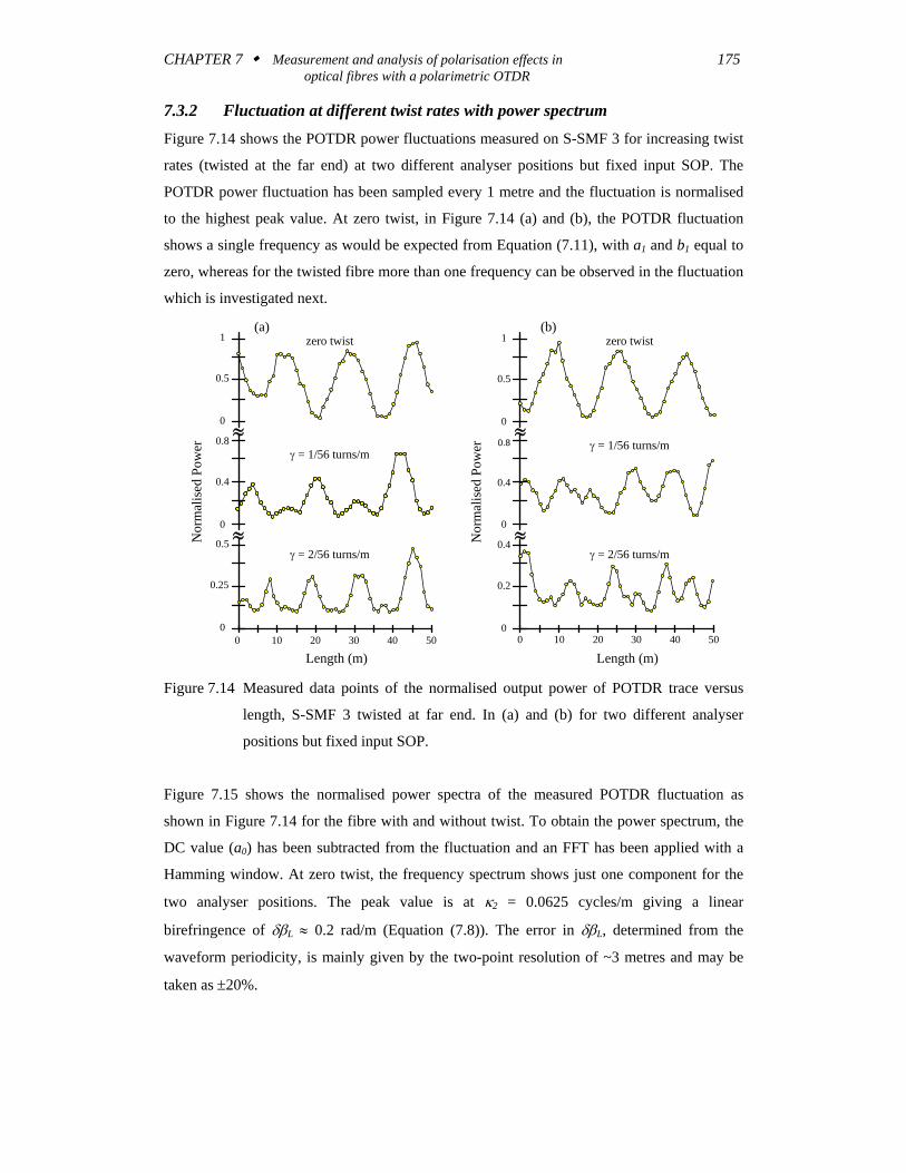
7.3.2 Fluctuation at different twist rates with power spectrum
Figure 7.14 shows the POTDR power fluctuations measured on S-SMF 3 for increasing twist
rates (twisted at the far end) at two different analyser positions but fixed input SOP. The
POTDR power fluctuation has been sampled every 1 metre and the fluctuation is normalised
to the highest peak value. At zero twist, in Figure 7.14 (a) and (b), the POTDR fluctuation
shows a single frequency as would be expected from Equation (7.11), with a1 and b1 equal to
zero, whereas for the twisted fibre more than one frequency can be observed in the fluctuation
which is investigated next.
30 4010 20 500
Nor
mal
ised
Pow
er
Nor
mal
ised
Pow
er
Length (m)
≈
0
0.5
0.25
0
0.8
0.4
≈0
1
0.5
zero twist
γ = 1/56 turns/m
γ = 2/56 turns/m
(a)
30 4010 20 500
Length (m)
0
0.4
0.2
0
0.8
0.4
0
1
0.5
≈
≈
zero twist
γ = 1/56 turns/m
γ = 2/56 turns/m
(b)
Figure 7.14 Measured data points of the normalised output power of POTDR trace versus
length, S-SMF 3 twisted at far end. In (a) and (b) for two different analyser
positions but fixed input SOP.
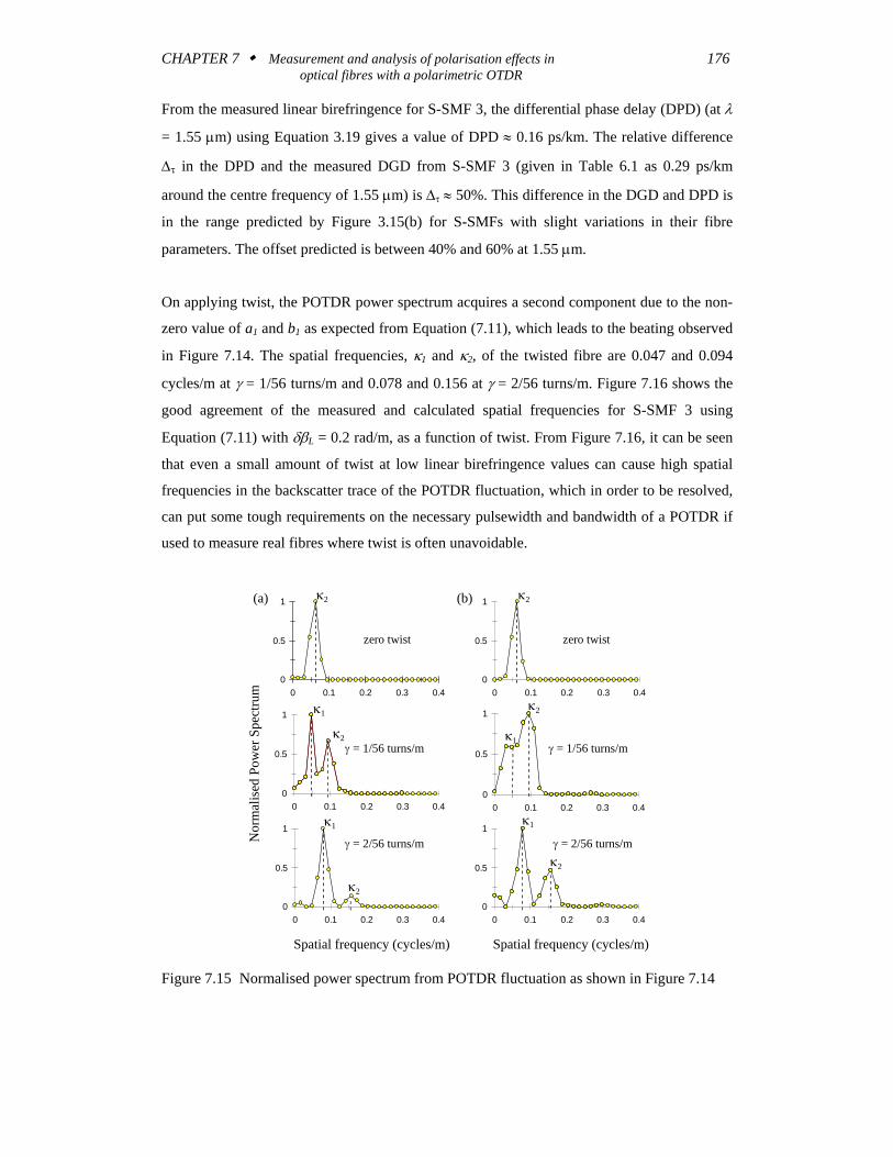
Figure 7.15 shows the normalised power spectra of the measured POTDR fluctuation as
shown in Figure 7.14 for the fibre with and without twist. To obtain the power spectrum, the
DC value (a0) has been subtracted from the fluctuation and an FFT has been applied with a
Hamming window. At zero twist, the frequency spectrum shows just one component for the
two analyser positions. The peak value is at κ2 = 0.0625 cycles/m giving a linear
birefringence of δβL ≈ 0.2 rad/m (Equation (7.8)). The error in δβL, determined from the
waveform periodicity, is mainly given by the two-point resolution of ~3 metres and may be
taken as ±20%.
CHAPTER 7 Measurement and analysis of polarisation effects in 176 optical fibres with a polarimetric OTDR
From the measured linear birefringence for S-SMF 3, the differential phase delay (DPD) (at λ
= 1.55 μm) using Equation 3.19 gives a value of DPD ≈ 0.16 ps/km. The relative difference
Δτ in the DPD and the measured DGD from S-SMF 3 (given in Table 6.1 as 0.29 ps/km
around the centre frequency of 1.55 μm) is Δτ ≈ 50%. This difference in the DGD and DPD is
in the range predicted by Figure 3.15(b) for S-SMFs with slight variations in their fibre
parameters. The offset predicted is between 40% and 60% at 1.55 μm.
On applying twist, the POTDR power spectrum acquires a second component due to the non-
zero value of a1 and b1 as expected from Equation (7.11), which leads to the beating observed
in Figure 7.14. The spatial frequencies, κ1 and κ2, of the twisted fibre are 0.047 and 0.094
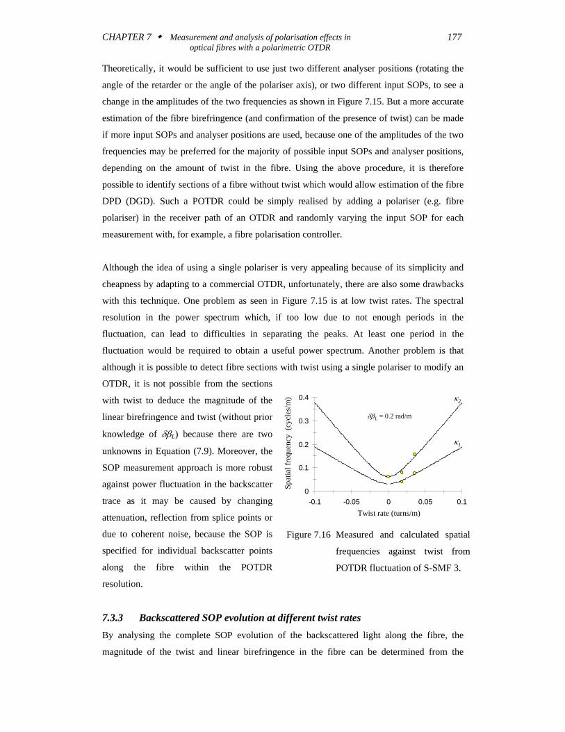
cycles/m at γ = 1/56 turns/m and 0.078 and 0.156 at γ = 2/56 turns/m. Figure 7.16 shows the
good agreement of the measured and calculated spatial frequencies for S-SMF 3 using
Equation (7.11) with δβL = 0.2 rad/m, as a function of twist. From Figure 7.16, it can be seen
that even a small amount of twist at low linear birefringence values can cause high spatial
frequencies in the backscatter trace of the POTDR fluctuation, which in order to be resolved,
can put some tough requirements on the necessary pulsewidth and bandwidth of a POTDR if
used to measure real fibres where twist is often unavoidable.
Spatial frequency (cycles/m)
Nor
mal
ised
Pow
er S
pect
rum
0
0.5
1
0 0.1 0.2 0.3 0.40
0.5
1
0 0.1 0.2 0.3 0.4
0
0.5
1
0 0.1 0.2 0.3 0.40
0.5
1
0 0.1 0.2 0.3 0.4
0
0.5
1
0 0.1 0.2 0.3 0.40
0.5
1
0 0.1 0.2 0.3 0.4
κ2 κ2
κ2
κ1κ2
κ1
κ2
κ1
κ2
κ1
zero twist zero twist
γ = 1/56 turns/m
γ = 2/56 turns/m
γ = 1/56 turns/m
γ = 2/56 turns/m
(a) (b)
Spatial frequency (cycles/m)
Figure 7.15 Normalised power spectrum from POTDR fluctuation as shown in Figure 7.14
CHAPTER 7 Measurement and analysis of polarisation effects in 177 optical fibres with a polarimetric OTDR
Theoretically, it would be sufficient to use just two different analyser positions (rotating the
angle of the retarder or the angle of the polariser axis), or two different input SOPs, to see a
change in the amplitudes of the two frequencies as shown in Figure 7.15. But a more accurate
estimation of the fibre birefringence (and confirmation of the presence of twist) can be made
if more input SOPs and analyser positions are used, because one of the amplitudes of the two
frequencies may be preferred for the majority of possible input SOPs and analyser positions,
depending on the amount of twist in the fibre. Using the above procedure, it is therefore
possible to identify sections of a fibre without twist which would allow estimation of the fibre
DPD (DGD). Such a POTDR could be simply realised by adding a polariser (e.g. fibre
polariser) in the receiver path of an OTDR and randomly varying the input SOP for each
measurement with, for example, a fibre polarisation controller.
Although the idea of using a single polariser is very appealing because of its simplicity and
cheapness by adapting to a commercial OTDR, unfortunately, there are also some drawbacks
with this technique. One problem as seen in Figure 7.15 is at low twist rates. The spectral
resolution in the power spectrum which, if too low due to not enough periods in the
fluctuation, can lead to difficulties in separating the peaks. At least one period in the
fluctuation would be required to obtain a useful power spectrum. Another problem is that
although it is possible to detect fibre sections with twist using a single polariser to modify an
OTDR, it is not possible from the sections
with twist to deduce the magnitude of the
linear birefringence and twist (without prior
knowledge of δβL) because there are two
unknowns in Equation (7.9). Moreover, the
SOP measurement approach is more robust
against power fluctuation in the backscatter
trace as it may be caused by changing
attenuation, reflection from splice points or
due to coherent noise, because the SOP is
specified for individual backscatter points
along the fibre within the POTDR
resolution.
7.3.3 Backscattered SOP evolution at different twist rates
By analysing the complete SOP evolution of the backscattered light along the fibre, the
magnitude of the twist and linear birefringence in the fibre can be determined from the
0
0.1
0.2
0.3
0.4
-0.1 -0.05 0 0.05 0.1Twist rate (turns/m)
Spa
tial f
requ
ency
(cyc
les/
m
δβL = 0.2 rad/m
Spat
ial f
requ
ency
(cy
cles
/m)
Twist rate (turns/m)
κ1
κ2
Figure 7.16 Measured and calculated spatial
frequencies against twist from
POTDR fluctuation of S-SMF 3.
CHAPTER 7 Measurement and analysis of polarisation effects in 178 optical fibres with a polarimetric OTDR
periodicity of the backscattered SOP evolution (Equation (7.9)), and by using the additional
information of the shape of the SOP evolution on the Poincaré sphere (Equation (7.10)), as
will be shown next.
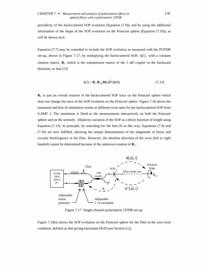
Equation (7.7) may be extended to include the SOP evolution as measured with the POTDR
set-up, shown in Figure 7.17, by multiplying the backscattered SOP, ss( )l , with a constant
rotation matrix, RC which is the transmission matrix of the 3 dB coupler in the backward
direction, so that [15]
s r rs R R M s( ) ( ) ( )l lC M= δβ 0 (7.13)
RC is just an overall rotation of the backscattered SOP trace on the Poincaré sphere which
does not change the trace of the SOP evolution on the Poincaré sphere. Figure 7.18 shows the
measured and best fit simulation results at different twist rates for the backscattered SOP from
S-SMF 3. The simulation is fitted to the measurements interactively on both the Poincaré
sphere and on the azimuth - ellipticity variation of the SOP as a direct function of length using
Equation (7.13). In principle, by searching for the best fit in this way, Equations (7.9) and
(7.10) are now fulfilled, allowing the unique determination of the magnitude of linear and
circular birefringence in the fibre. However, the absolute direction of the twist (left or right
handed) cannot be determined because of the unknown rotation of RC.
Adjustableλ /4 waveplate
Adjustablelinearpolariser
25nsFibre under test
RotationStageSOP in
OTDRDFB
EDFAPC
3 dBcoupler
( )R lFδβr
( )R lTFδβr
RC
RM
Figure 7.17 Single-channel polarimetric OTDR set-up.
Figure 7.18(a) shows the SOP evolution on the Poincaré sphere for the fibre in the zero twist
condition, defined as that giving maximum DGD (see Section 6.2).
CHAPTER 7 Measurement and analysis of polarisation effects in 179 optical fibres with a polarimetric OTDR
H
P
H
Q
H
Q
γ = 0 turns/m γ = 0.01 turns/m γ = 0.019 turns/m
Measurement from first 19mMeasurement from last 31m
Simulation Start point of the measurement
RCP RCPRCP(a) (b) (c)
-90
-60
-30
0
30
60
90
0 5 10 15 20 25 30 35Length (m)
Azim
uth
(deg
)
-90
-60
-30
0
30
60
90
0 5 10 15 20 25 30 35Length (m)
Azim
uth
(deg
)
-45
-30
-15
0
15
30
0 5 10 15 20 25 30 35Length (m)
Ellip
ticity
(deg
)
δβL = 0.19 rad/m γ = 0 turns/m
δβL = 0.19 rad/m γ = 0 turns/m
δβL = 0.19 rad/m γ = 0.01 turns/m
δβL = 0.19 rad/m γ = 0.01 turns/m
(d)
(e)
-45
-30
-15
0
15
30
0 5 10 15 20 25 30 35Length (m)
Ellip
ticity
(deg
)
Measurement from last 31mSimulation
(f)
-90
-60
-30
0
30
60
90
0 5 10 15 20 25 30 35Length (m)
Azi
mut
h (d
eg)
-40
-30
-20
-10
0
10
20
0 5 10 15 20 25 30 35Length (m)
Ellip
ticity
(deg
)
δβL = 0.19 rad/m γ = 0.019 turns/m
δβL = 0.19 rad/m γ = 0.019 turns/m
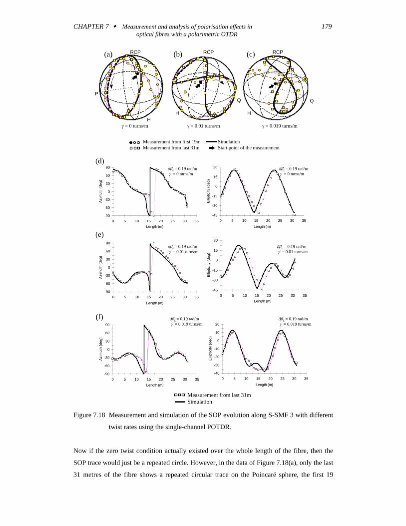
Figure 7.18 Measurement and simulation of the SOP evolution along S-SMF 3 with different
twist rates using the single-channel POTDR.
Now if the zero twist condition actually existed over the whole length of the fibre, then the
SOP trace would just be a repeated circle. However, in the data of Figure 7.18(a), only the last
31 metres of the fibre shows a repeated circular trace on the Poincaré sphere, the first 19
CHAPTER 7 Measurement and analysis of polarisation effects in 180 optical fibres with a polarimetric OTDR
metres giving data points away from the circle. From this, and measuring the fibre with left
and right hand twist using the POTDR (see Subsection 7.3.6), it could be concluded that the
fibre possesses some small non-uniform twist which may be frozen in during the fibre
fabrication process (the small non-uniform twist in the first 19 metres of fibre has been found
to be < 0.2/56 turns/m).
The last 31 metres of fibre was then modelled as a section with zero twist and constant linear
birefringence as the variable to find the best fit to the measurement by using Equation (7.13).
The best fit simulation, indicated in Figure 7.18 (a) and (d), was obtained for δβL = 0.19 rad/m
for the last 31 metres of fibre, which is within 5% of the value estimated from the power
spectrum for the total 50 metre fibre length in Figure 7.15(a), and is within the error expected
for the POTDR resolution. In applying a twist of 0.01 turns/m, Figure 7.18 (b) and (e), the
backscattered SOP of the last 31 metres of fibre traces a figure of eight shape in accordance
with Equation (7.12). For the higher applied twist rate of 0.019 turns/m, Figure 7.18 (c) and
(f), the area of the figure eight decreases as predicted in Figure 7.13 (c) to (d) by using
Equation (7.12). The simulation traces for these two twist values, Figure 7.18 (b) and (e) and
Figure 7.18 (c) and (f), again give δβL = 0.19 rad/m and twist values of 0.012 and 0.021
turns/m respectively for the best fit. The error in the twist estimated with POTDR is < 20%
for the two mechanically applied twist rates.
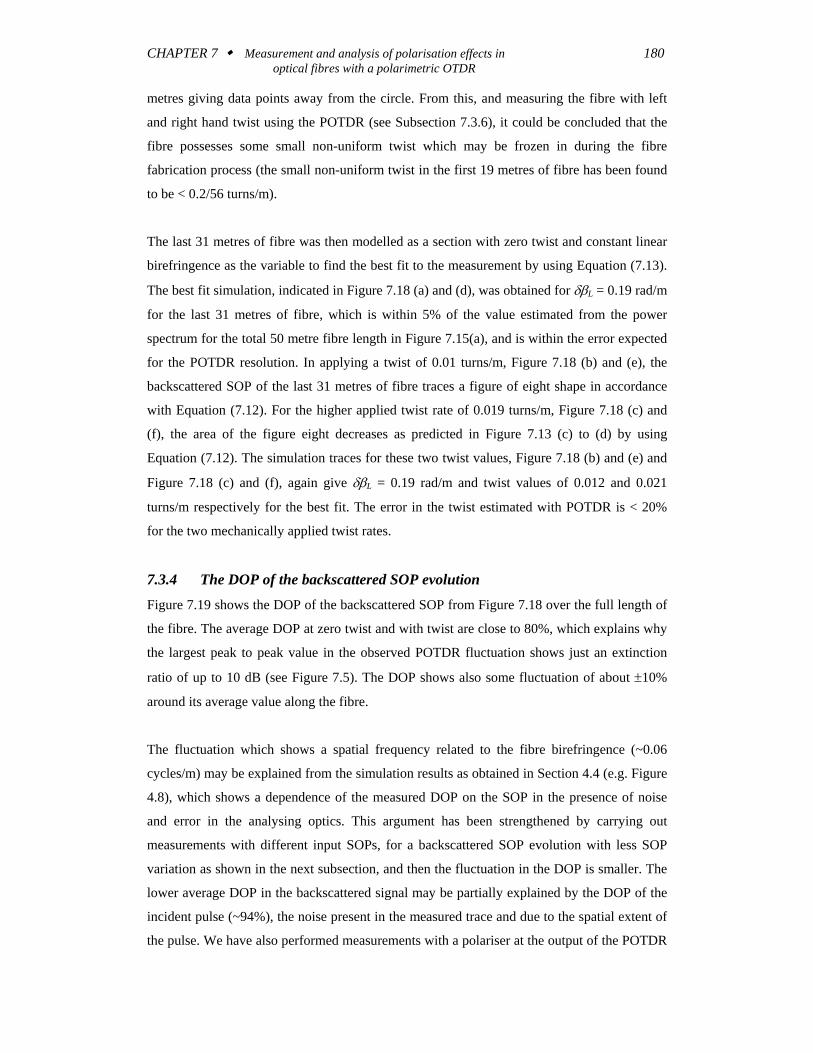
7.3.4 The DOP of the backscattered SOP evolution
Figure 7.19 shows the DOP of the backscattered SOP from Figure 7.18 over the full length of
the fibre. The average DOP at zero twist and with twist are close to 80%, which explains why
the largest peak to peak value in the observed POTDR fluctuation shows just an extinction
ratio of up to 10 dB (see Figure 7.5). The DOP shows also some fluctuation of about ±10%
around its average value along the fibre.
The fluctuation which shows a spatial frequency related to the fibre birefringence (~0.06
cycles/m) may be explained from the simulation results as obtained in Section 4.4 (e.g. Figure
4.8), which shows a dependence of the measured DOP on the SOP in the presence of noise
and error in the analysing optics. This argument has been strengthened by carrying out
measurements with different input SOPs, for a backscattered SOP evolution with less SOP
variation as shown in the next subsection, and then the fluctuation in the DOP is smaller. The
lower average DOP in the backscattered signal may be partially explained by the DOP of the
incident pulse (~94%), the noise present in the measured trace and due to the spatial extent of
the pulse. We have also performed measurements with a polariser at the output of the POTDR
CHAPTER 7 Measurement and analysis of polarisation effects in 181 optical fibres with a polarimetric OTDR
(Setion 7.4 and Appendix B), which ensures that the injected pulse into the fibre is ~100%
polarised, and the backscattered DOP nevertheless showed an average DOP of around 80%. It
is interesting that this 80% DOP has also been reported in Reference [197] using a
polarimetric OTDR, although this was measured at λ ~ 0.5 μm. This lower DOP, we could
conclude, may be inherent to some degree (more or less depending on the noise and error in
the used system) in the fibre scattering process itself which has been assumed ideal in the
theory, but needs further investigation. In general, a lower DOP is not desired as it increases
the error in the measured SOP in the presence of noise as discussed in Section 4.4.
0
0.2
0.4
0.6
0.8
1
0 10 20 30 40 50Length (m)
DO
P
0
0.2
0.4
0.6
0.8
1
0 10 20 30 40 50Length (m)
DO
P
0
0.2
0.4
0.6
0.8
1
0 10 20 30 40 50Length (m)
DO
P
γ = 0 turns/m⟨DOPM⟩ = 0.79
γ = 0.01 turns/m⟨DOP⟩ = 0.79
γ = 0.019 turns/m⟨DOP⟩ = 0.76
S-SMF 3:Measured DOPAverage DOP
(a) (b)
(c)
Figure 7.19 The DOP of the backscattered SOP as shown in Figure 7.18 for the different
twist rates.
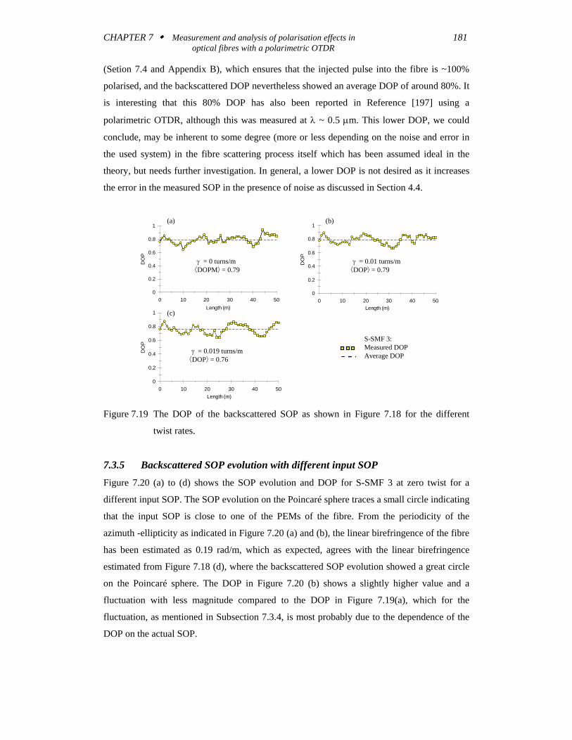
7.3.5 Backscattered SOP evolution with different input SOP
Figure 7.20 (a) to (d) shows the SOP evolution and DOP for S-SMF 3 at zero twist for a
different input SOP. The SOP evolution on the Poincaré sphere traces a small circle indicating
that the input SOP is close to one of the PEMs of the fibre. From the periodicity of the
azimuth -ellipticity as indicated in Figure 7.20 (a) and (b), the linear birefringence of the fibre
has been estimated as 0.19 rad/m, which as expected, agrees with the linear birefringence
estimated from Figure 7.18 (d), where the backscattered SOP evolution showed a great circle
on the Poincaré sphere. The DOP in Figure 7.20 (b) shows a slightly higher value and a
fluctuation with less magnitude compared to the DOP in Figure 7.19(a), which for the
fluctuation, as mentioned in Subsection 7.3.4, is most probably due to the dependence of the
DOP on the actual SOP.
CHAPTER 7 Measurement and analysis of polarisation effects in 182 optical fibres with a polarimetric OTDR
Measurement from last 31m
0
20
40
60
0 5 10 15 20 25 30 35Length (m)
Azi
mut
h (d
eg)
-30
-20
-10
0
10
0 5 10 15 20 25 30 35Length (m)
Ellip
ticity
(deg
)
0
0.2
0.4
0.6
0.8
1
0 5 10 15 20 25 30 35Length (m)
DO
P
δβL = 0.19 rad/m γ = 0 turns/m
δβL = 0.19 rad/m γ = 0 turns/m
L = 16.8 m
RCP
H
P
L = 16.8 m
γ = 0 turns/m⟨DOP⟩ = 0.83
(a) (b)
(c) (d)
Figure 7.20 Measurement of the backscattered SOP evolution at zero twist along S-SMF 3
with input SOP close to one of the PEMs of the fibre.
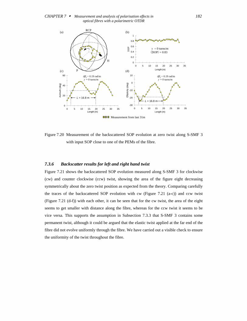
7.3.6 Backscatter results for left and right hand twist
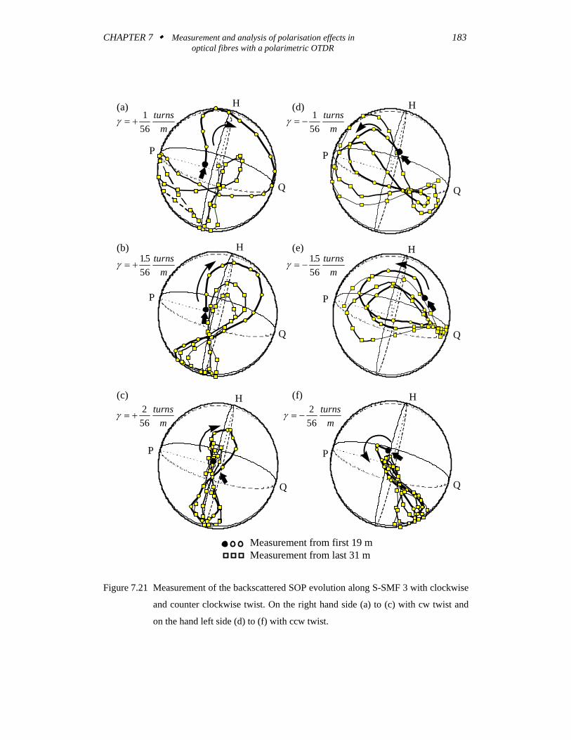
Figure 7.21 shows the backscattered SOP evolution measured along S-SMF 3 for clockwise
(cw) and counter clockwise (ccw) twist, showing the area of the figure eight decreasing
symmetrically about the zero twist position as expected from the theory. Comparing carefully
the traces of the backscattered SOP evolution with cw (Figure 7.21 (a-c)) and ccw twist
(Figure 7.21 (d-f)) with each other, it can be seen that for the cw twist, the area of the eight
seems to get smaller with distance along the fibre, whereas for the ccw twist it seems to be
vice versa. This supports the assumption in Subsection 7.3.3 that S-SMF 3 contains some
permanent twist, although it could be argued that the elastic twist applied at the far end of the
fibre did not evolve uniformly through the fibre. We have carried out a visible check to ensure
the uniformity of the twist throughout the fibre.
CHAPTER 7 Measurement and analysis of polarisation effects in 183 optical fibres with a polarimetric OTDR
Measurement from first 19 mMeasurement from last 31 m
(a) H
P
Q
γ = +1
56turns
m
(d)γ = −
156
turnsm
(b) H
P
Q
γ = +1556. turns
m
(e)γ = −
1556. turns
m
H
P
Q
H
P
Q
(c) H
P
Q
γ = +256
turnsm
(f) H
P
Q
γ = −256
turnsm
Figure 7.21 Measurement of the backscattered SOP evolution along S-SMF 3 with clockwise
and counter clockwise twist. On the right hand side (a) to (c) with cw twist and
on the hand left side (d) to (f) with ccw twist.
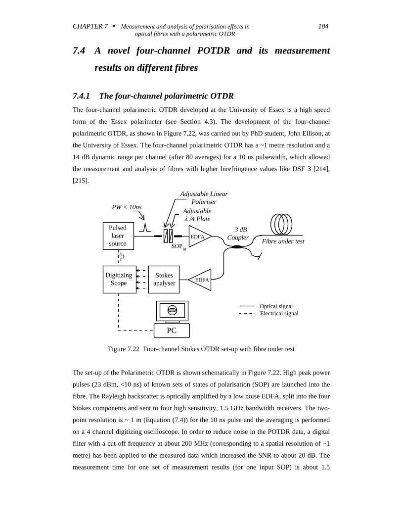
CHAPTER 7 Measurement and analysis of polarisation effects in 184 optical fibres with a polarimetric OTDR
7.4 A novel four-channel POTDR and its measurement
results on different fibres
7.4.1 The four-channel polarimetric OTDR The four-channel polarimetric OTDR developed at the University of Essex is a high speed
form of the Essex polarimeter (see Section 4.3). The development of the four-channel
polarimetric OTDR, as shown in Figure 7.22, was carried out by PhD student, John Ellison, at
the University of Essex. The four-channel polarimetric OTDR has a ~1 metre resolution and a
14 dB dynamic range per channel (after 80 averages) for a 10 ns pulsewidth, which allowed
the measurement and analysis of fibres with higher birefringence values like DSF 3 [214],
[215].
Adjustableλ /4 Plate
Adjustable LinearPolariser
Pulsedlaser
source
PW < 10ns
3 dBCoupler
SOPin
EDFA
EDFAStokes
analyserDigitizing
Scope
Fibre under test
Optical signal Electrical signal
PC
Figure 7.22 Four-channel Stokes OTDR set-up with fibre under test
The set-up of the Polarimetric OTDR is shown schematically in Figure 7.22. High peak power
pulses (23 dBm, <10 ns) of known sets of states of polarisation (SOP) are launched into the
fibre. The Rayleigh backscatter is optically amplified by a low noise EDFA, split into the four
Stokes components and sent to four high sensitivity, 1.5 GHz bandwidth receivers. The two-
point resolution is ~ 1 m (Equation (7.4)) for the 10 ns pulse and the averaging is performed
on a 4 channel digitizing oscilloscope. In order to reduce noise in the POTDR data, a digital
filter with a cut-off frequency at about 200 MHz (corresponding to a spatial resolution of ~1
metre) has been applied to the measured data which increased the SNR to about 20 dB. The
measurement time for one set of measurement results (for one input SOP) is about 1.5
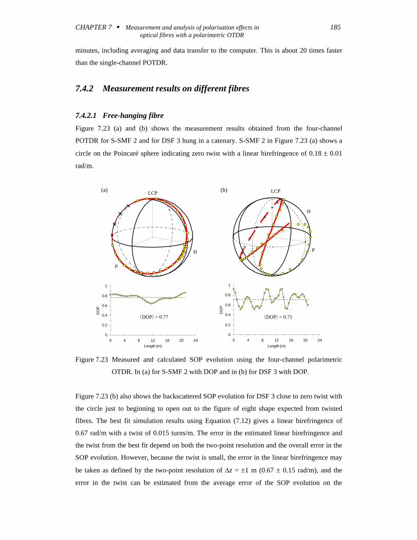
CHAPTER 7 Measurement and analysis of polarisation effects in 185 optical fibres with a polarimetric OTDR
minutes, including averaging and data transfer to the computer. This is about 20 times faster
than the single-channel POTDR.
7.4.2 Measurement results on different fibres
7.4.2.1 Free-hanging fibre
Figure 7.23 (a) and (b) shows the measurement results obtained from the four-channel
POTDR for S-SMF 2 and for DSF 3 hung in a catenary. S-SMF 2 in Figure 7.23 (a) shows a
circle on the Poincaré sphere indicating zero twist with a linear birefringence of 0.18 ± 0.01
rad/m.
LCP
H
P
(a)
0
0.2
0.4
0.6
0.8
1
0 4 8 12 16 20 24Length (m)
DO
P
⟨DOP⟩ = 0.77
LCP
H
P
0
0.2
0.4
0.6
0.8
1
0 4 8 12 16 20 24Length (m)
DO
P
⟨DOP⟩ = 0.71
(b)
Figure 7.23 Measured and calculated SOP evolution using the four-channel polarimetric
OTDR. In (a) for S-SMF 2 with DOP and in (b) for DSF 3 with DOP.
Figure 7.23 (b) also shows the backscattered SOP evolution for DSF 3 close to zero twist with
the circle just to beginning to open out to the figure of eight shape expected from twisted
fibres. The best fit simulation results using Equation (7.12) gives a linear birefringence of
0.67 rad/m with a twist of 0.015 turns/m. The error in the estimated linear birefringence and
the twist from the best fit depend on both the two-point resolution and the overall error in the
SOP evolution. However, because the twist is small, the error in the linear birefringence may
be taken as defined by the two-point resolution of Δz = ±1 m (0.67 ± 0.15 rad/m), and the
error in the twist can be estimated from the average error of the SOP evolution on the
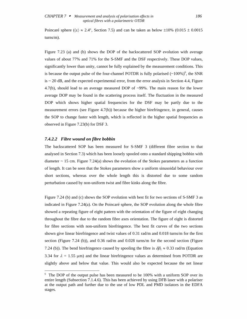
CHAPTER 7 Measurement and analysis of polarisation effects in 186 optical fibres with a polarimetric OTDR
Poincaré sphere (⟨ε⟩ ≈ 2.4°, Section 7.5) and can be taken as below ±10% (0.015 ± 0.0015
turns/m).
Figure 7.23 (a) and (b) shows the DOP of the backscattered SOP evolution with average
values of about 77% and 71% for the S-SMF and the DSF respectively. These DOP values,
significantly lower than unity, cannot be fully explained by the measurement conditions. This
is because the output pulse of the four-channel POTDR is fully polarised (~100%)6, the SNR
is ~ 20 dB, and the expected experimental error, from the error analysis in Section 4.4, Figure
4.7(b), should lead to an average measured DOP of ~99%. The main reason for the lower
average DOP may be found in the scattering process itself. The fluctuation in the measured
DOP which shows higher spatial frequencies for the DSF may be partly due to the
measurement errors (see Figure 4.7(b)) because the higher birefringence, in general, causes
the SOP to change faster with length, which is reflected in the higher spatial frequencies as
observed in Figure 7.23(b) for DSF 3.
7.4.2.2 Fibre wound on fibre bobbin
The backscattered SOP has been measured for S-SMF 3 (different fibre section to that
analysed in Section 7.3) which has been loosely spooled onto a standard shipping bobbin with
diameter ~ 15 cm. Figure 7.24(a) shows the evolution of the Stokes parameters as a function
of length. It can be seen that the Stokes parameters show a uniform sinusoidal behaviour over
short sections, whereas over the whole length this is distorted due to some random
perturbation caused by non-uniform twist and fibre kinks along the fibre.
Figure 7.24 (b) and (c) shows the SOP evolution with best fit for two sections of S-SMF 3 as
indicated in Figure 7.24(a). On the Poincaré sphere, the SOP evolution along the whole fibre
showed a repeating figure of eight pattern with the orientation of the figure of eight changing
throughout the fibre due to the random fibre axes orientation. The figure of eight is distorted
for fibre sections with non-uniform birefringence. The best fit curves of the two sections
shown give linear birefringence and twist values of 0.31 rad/m and 0.018 turns/m for the first
section (Figure 7.24 (b)), and 0.36 rad/m and 0.028 turns/m for the second section (Figure
7.24 (b)). The bend birefringence caused by spooling the fibre is δβL ≈ 0.33 rad/m (Equation
3.34 for λ = 1.55 μm) and the linear birefringence values as determined from POTDR are
slightly above and below that value. This would also be expected because the net linear
6 The DOP of the output pulse has been measured to be 100% with a uniform SOP over its entire length (Subsection 7.1.4.6). This has been achieved by using DFB laser with a polariser at the output path and further due to the use of low PDL and PMD isolators in the EDFA stages.
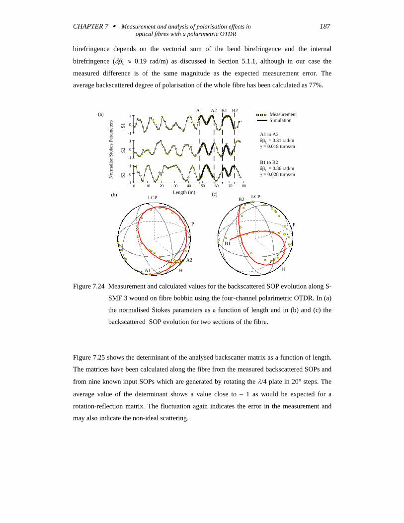
CHAPTER 7 Measurement and analysis of polarisation effects in 187 optical fibres with a polarimetric OTDR
birefringence depends on the vectorial sum of the bend birefringence and the internal
birefringence (δβL ≈ 0.19 rad/m) as discussed in Section 5.1.1, although in our case the
measured difference is of the same magnitude as the expected measurement error. The
average backscattered degree of polarisation of the whole fibre has been calculated as 77%.
B1A1 B2A2N
orm
alise
Sto
kes P
aram
eter
s
S1
Length (m)
S3S2
-1
0
1
-1
0
1
0 10 20 30 40 50 60 70 80
-1
0
1
MeasurementSimulation
B1 to B2δβL = 0.36 rad/mγ = 0.028 turns/m
A1 to A2δβL = 0.31 rad/mγ = 0.018 turns/m
(a)
LCP
P
H
B1
B2(c)
LCP
P
H
A2
(b)
A1
Figure 7.24 Measurement and calculated values for the backscattered SOP evolution along S-
SMF 3 wound on fibre bobbin using the four-channel polarimetric OTDR. In (a)
the normalised Stokes parameters as a function of length and in (b) and (c) the
backscattered SOP evolution for two sections of the fibre.
Figure 7.25 shows the determinant of the analysed backscatter matrix as a function of length.
The matrices have been calculated along the fibre from the measured backscattered SOPs and
from nine known input SOPs which are generated by rotating the λ/4 plate in 20° steps. The
average value of the determinant shows a value close to − 1 as would be expected for a
rotation-reflection matrix. The fluctuation again indicates the error in the measurement and
may also indicate the non-ideal scattering.
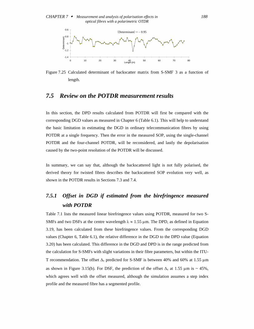
CHAPTER 7 Measurement and analysis of polarisation effects in 188 optical fibres with a polarimetric OTDR
⟨Determinant⟩ = − 0.95
-1.4
-1.2
-1
-0.8
-0.6
0 10 20 30 40 50 60 70 80Length (m)
Det
erm
inan
t
Figure 7.25 Calculated determinant of backscatter matrix from S-SMF 3 as a function of
length.
7.5 Review on the POTDR measurement results
In this section, the DPD results calculated from POTDR will first be compared with the
corresponding DGD values as measured in Chapter 6 (Table 6.1). This will help to understand
the basic limitation in estimating the DGD in ordinary telecommunication fibres by using
POTDR at a single frequency. Then the error in the measured SOP, using the single-channel
POTDR and the four-channel POTDR, will be reconsidered, and lastly the depolarisation
caused by the two-point resolution of the POTDR will be discussed.
In summary, we can say that, although the backscattered light is not fully polarised, the
derived theory for twisted fibres describes the backscattered SOP evolution very well, as
shown in the POTDR results in Sections 7.3 and 7.4.
7.5.1 Offset in DGD if estimated from the birefringence measured
with POTDR Table 7.1 lists the measured linear birefringence values using POTDR, measured for two S-
SMFs and two DSFs at the centre wavelength λ ≈ 1.55 μm. The DPD, as defined in Equation
3.19, has been calculated from these birefringence values. From the corresponding DGD
values (Chapter 6, Table 6.1), the relative difference in the DGD to the DPD value (Equation
3.20) has been calculated. This difference in the DGD and DPD is in the range predicted from
the calculation for S-SMFs with slight variations in their fibre parameters, but within the ITU-
T recommendation. The offset Δτ predicted for S-SMF is between 40% and 60% at 1.55 μm
as shown in Figure 3.15(b). For DSF, the prediction of the offset Δτ at 1.55 μm is ~ 45%,
which agrees well with the offset measured, although the simulation assumes a step index
profile and the measured fibre has a segmented profile.
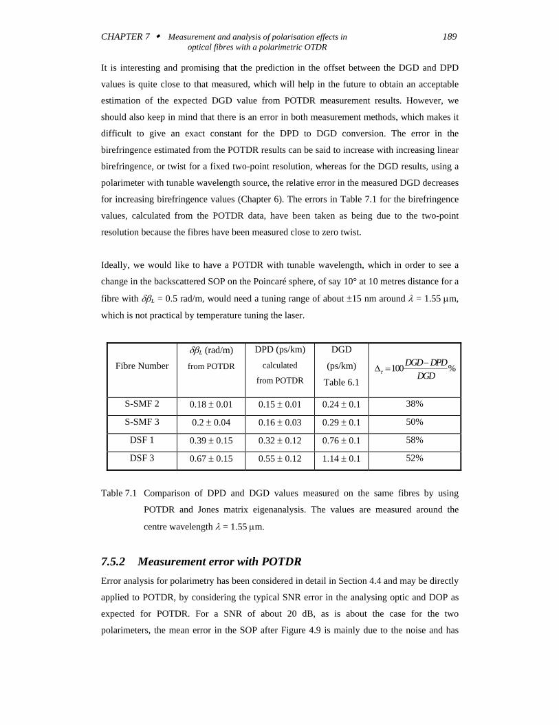
CHAPTER 7 Measurement and analysis of polarisation effects in 189 optical fibres with a polarimetric OTDR
It is interesting and promising that the prediction in the offset between the DGD and DPD
values is quite close to that measured, which will help in the future to obtain an acceptable
estimation of the expected DGD value from POTDR measurement results. However, we
should also keep in mind that there is an error in both measurement methods, which makes it
difficult to give an exact constant for the DPD to DGD conversion. The error in the
birefringence estimated from the POTDR results can be said to increase with increasing linear
birefringence, or twist for a fixed two-point resolution, whereas for the DGD results, using a
polarimeter with tunable wavelength source, the relative error in the measured DGD decreases
for increasing birefringence values (Chapter 6). The errors in Table 7.1 for the birefringence
values, calculated from the POTDR data, have been taken as being due to the two-point
resolution because the fibres have been measured close to zero twist.
Ideally, we would like to have a POTDR with tunable wavelength, which in order to see a
change in the backscattered SOP on the Poincaré sphere, of say 10° at 10 metres distance for a
fibre with δβL = 0.5 rad/m, would need a tuning range of about ±15 nm around λ = 1.55 μm,
which is not practical by temperature tuning the laser.
Fibre Number
δβL (rad/m)
from POTDR
DPD (ps/km)
calculated
from POTDR
DGD
(ps/km)
Table 6.1
Δτ =−100DGD DPD
DGD%
S-SMF 2 0.18 ± 0.01 0.15 ± 0.01 0.24 ± 0.1 38%
S-SMF 3 0.2 ± 0.04 0.16 ± 0.03 0.29 ± 0.1 50%
DSF 1 0.39 ± 0.15 0.32 ± 0.12 0.76 ± 0.1 58%
DSF 3 0.67 ± 0.15 0.55 ± 0.12 1.14 ± 0.1 52%
Table 7.1 Comparison of DPD and DGD values measured on the same fibres by using
POTDR and Jones matrix eigenanalysis. The values are measured around the
centre wavelength λ = 1.55 μm.
7.5.2 Measurement error with POTDR Error analysis for polarimetry has been considered in detail in Section 4.4 and may be directly
applied to POTDR, by considering the typical SNR error in the analysing optic and DOP as
expected for POTDR. For a SNR of about 20 dB, as is about the case for the two
polarimeters, the mean error in the SOP after Figure 4.9 is mainly due to the noise and has
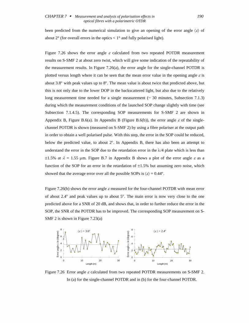
CHAPTER 7 Measurement and analysis of polarisation effects in 190 optical fibres with a polarimetric OTDR
been predicted from the numerical simulation to give an opening of the error angle ⟨ε⟩ of
about 2° (for overall errors in the optics < 1° and fully polarised light).
Figure 7.26 shows the error angle ε calculated from two repeated POTDR measurement
results on S-SMF 2 at about zero twist, which will give some indication of the repeatability of
the measurement results. In Figure 7.26(a), the error angle for the single-channel POTDR is
plotted versus length where it can be seen that the mean error value in the opening angle ε is
about 3.8° with peak values up to 8°. The mean value is about twice that predicted above, but
this is not only due to the lower DOP in the backscattered light, but also due to the relatively
long measurement time needed for a single measurement (~ 30 minutes, Subsection 7.1.3)
during which the measurement conditions of the launched SOP change slightly with time (see
Subsection 7.1.4.5). The corresponding SOP measurements for S-SMF 2 are shown in
Appendix B, Figure B.6(a). In Appendix B (Figure B.6(b)), the error angle ε of the single-
channel POTDR is shown (measured on S-SMF 2) by using a fibre polariser at the output path
in order to obtain a well polarised pulse. With this step, the error in the SOP could be reduced,
below the predicted value, to about 2°. In Appendix B, there has also been an attempt to
understand the error in the SOP due to the retardation error in the λ/4 plate which is less than
±1.5% at λ = 1.55 μm. Figure B.7 in Appendix B shows a plot of the error angle ε as a
function of the SOP for an error in the retardation of ±1.5% but assuming zero noise, which
showed that the average error over all the possible SOPs is ⟨ε⟩ = 0.44°.
Figure 7.26(b) shows the error angle ε measured for the four-channel POTDR with mean error
of about 2.4° and peak values up to about 5°. The main error is now very close to the one
predicted above for a SNR of 20 dB, and shows that, in order to further reduce the error in the
SOP, the SNR of the POTDR has to be improved. The corresponding SOP measurement on S-
SMF 2 is shown in Figure 7.23(a)
0
2
4
6
8
0 10 20 30Length (m)
Erro
r ang
le ε
in (d
egre
e)
Erro
r ang
le ε
in (d
egre
e)⟨ε ⟩ = 3.6° ⟨ε ⟩ = 2.4°
0
2
4
6
8
0 10 20 30Length (m)
Figure 7.26 Error angle ε calculated from two repeated POTDR measurements on S-SMF 2.
In (a) for the single-channel POTDR and in (b) for the four-channel POTDR.
CHAPTER 7 Measurement and analysis of polarisation effects in 191 optical fibres with a polarimetric OTDR
In the presence of twist, the backscattered SOP evolution can be characterised by the
periodicity of the SOP evolution, as defined in Equation (7.9), and by the shape of the SOP
evolution, if plotted on the Poincaré sphere, as defined in Equation (7.10). For zero twist, the
periodicity of the SOP evolution is determined by Equation (7.8) and the shape of the SOP
evolution is a circle on the sphere. Assuming now that the measured backscattered SOP show
one whole uniform evolution, the error in the linear and circular birefringence estimated from
the POTDR data may be categorised in the following way:
(i) The error in the SOP periodicity may be taken as about L ± ΔL ≈ L ± Δz with L given in
Equation (7.9) for fibre with twist and in Equation (7.8) without, and Δz is given in
Equation (7.4).
(ii) The error in the shape of the SOP evolution may be visualised as an error Δα in the angle
α of the resultant rotation vector in forward or backward direction (Equation (7.10)) so
that the average error in the measured SOP, away from the error free shape, is given by the
opening angle ⟨ε⟩ as α ± Δα ≈ α ± ⟨ε⟩/2. The error angle ⟨ε⟩ is difficult to specify directly
from the measurement conditions because it is an interplay of many errors, not only the
noise (SNR) and linearity of the instrument (Subsection 7.1.4.3), but also the stability of
the input SOP and the backscattered DOP. However, it may simply be determined as
shown in Figure 7.26, from consecutive measurement results as carried out for the two
POTDRs.
For the single-channel POTDR, the two-point resolution of about ±3 metres (Subsection
7.1.4.4) determines the error, at zero twist, for the estimated linear birefringence, which is the
error given in Table 7.1 for S-SMF 3 and DSF 1 (±1 metre for S-SMF 2 and DSF 3). In the
presence of twist, the error, as shown above, not only depends on the two-point resolution but
also on the uncertainty in the measured SOP evolution, and the error in the estimated linear
birefringence increases further with increasing twist.
7.5.3 Two-point resolution requirement as a function of the fibre
birefringence
Figure 7.27(a) shows the DOP calculated using Equation 2.10 and Equation 2.11 by
integrating the SOPs on the Poincaré sphere along arcs with different radii. For the arc with
radius one, which is a great circle on the Poincaré sphere, the integrated DOP shows fully
depolarised light for multiple rotations of 2π. For decreasing radius, the depolarisation as a
CHAPTER 7 Measurement and analysis of polarisation effects in 192 optical fibres with a polarimetric OTDR
function of the integration angle gets smaller and for zero radius which represents just one
point on the Poincaré sphere, the SOP stays fully polarised as expected for a fixed SOP. The
last case is interesting because it would represent the case if light is launched into one of the
PEMs of the fibre. Figure 7.27(b) shows the DOP for the measured backscattered SOP
evolution integrated along S-SMF 2 as a function of length, at zero twist for two different
input SOPs. For the first input SOP, which generated a circle in the backscattered SOP
evolution of radius ~0.9 (see Figure 7.23(a)), the DOP of the integrated SOP evolves from
about 0.85 to 0.2, with a minimum defined by the SOP periodicity at about L = 17 metre (δβL
≈ 0.18 ≈ π/L (rad/m)). For the other SOP, which generated a small circle with radius of about
0.46, the DOP of the integrated SOP is nearly fixed, as we would expect for such a small
radius. The lower start DOP (at l ≈ 0 m) in Figure 7.27(b) is due to the fact that the
backscattered light is not fully polarised (~ 80%, see Figure 7.23(a)).
It is interesting to note that, although there were many trials, it was never possible to find an
input SOP into the fibre under test perfectly aligned with the fibres PEMs. This may be due to
the fact that for the fibre, for a combined forward-backward travel path, such PEMs do not
exist due to the non-ideal scattering.
The inset in Figure 7.27(a) shows a magnified view of the DOP for the integrated SOP from
just 20° of the arc. The two-point resolution for the POTDR should be such that the SOP in
the fibre does not changes significantly within that range in order to obtain a DOP close to
one. As a rule of the thumb, we may define the maximum two-point resolution, Δz, for
POTDR assuming less than 20° angular movement on the Poincaré sphere as a function of the
fibre birefringence ( )δβ δβ γ γ= + −L g2 22
Δz <20360
πδβ
(7.14)
From Equation (7.14), we may calculate the two-point resolution needed in order to measure
an intrinsic linear birefringence of δβL = 3 rad/m, which is about the highest intrinsic linear
birefringence we would expect in most S-SMFs and DSFs (Table 6.1). The spatial resolution
needed would be about 0.06 metre. Further, as evident from Figure 4.9, for a POTDR we
would like to have a DR of at least 20 dB in order to measure reasonably accurate
backscattered SOPs along a fibre under test.
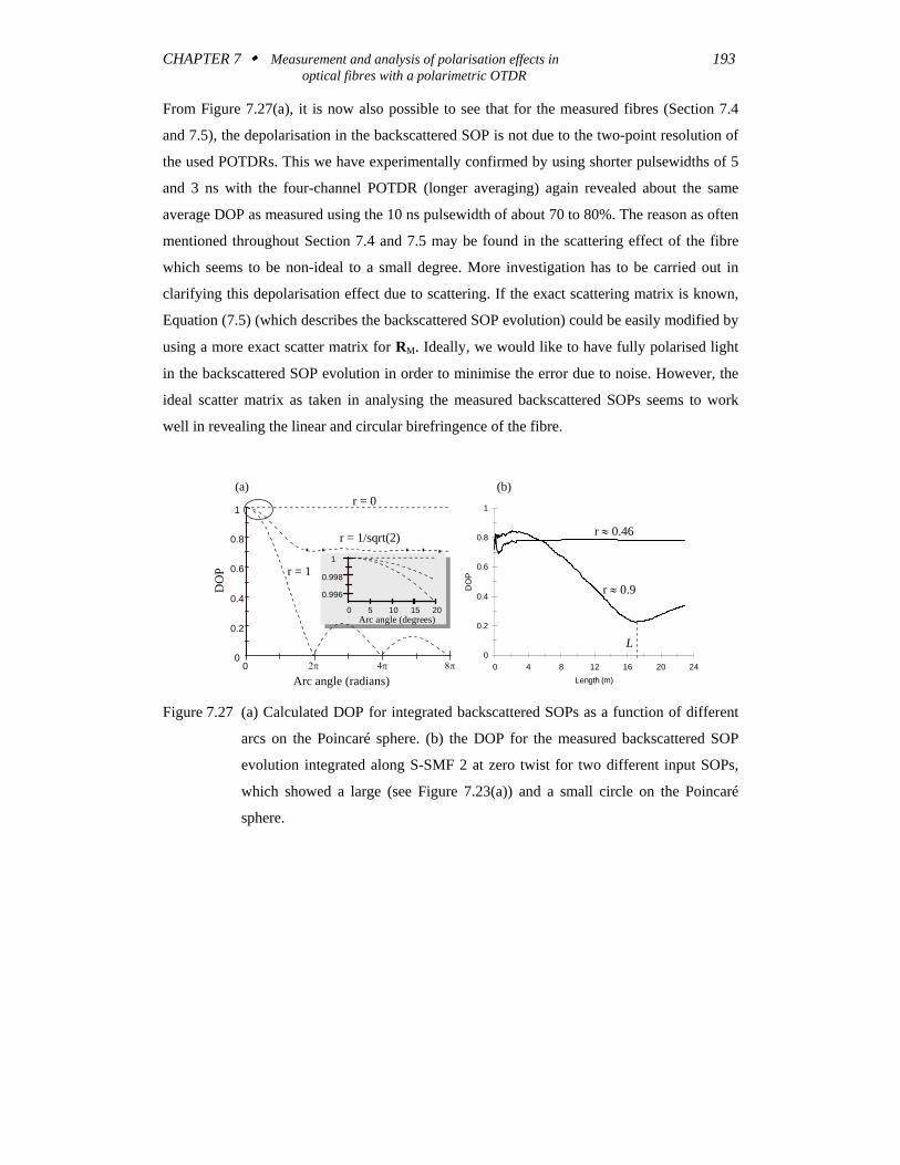
CHAPTER 7 Measurement and analysis of polarisation effects in 193 optical fibres with a polarimetric OTDR
From Figure 7.27(a), it is now also possible to see that for the measured fibres (Section 7.4
and 7.5), the depolarisation in the backscattered SOP is not due to the two-point resolution of
the used POTDRs. This we have experimentally confirmed by using shorter pulsewidths of 5
and 3 ns with the four-channel POTDR (longer averaging) again revealed about the same
average DOP as measured using the 10 ns pulsewidth of about 70 to 80%. The reason as often
mentioned throughout Section 7.4 and 7.5 may be found in the scattering effect of the fibre
which seems to be non-ideal to a small degree. More investigation has to be carried out in
clarifying this depolarisation effect due to scattering. If the exact scattering matrix is known,
Equation (7.5) (which describes the backscattered SOP evolution) could be easily modified by
using a more exact scatter matrix for RM. Ideally, we would like to have fully polarised light
in the backscattered SOP evolution in order to minimise the error due to noise. However, the
ideal scatter matrix as taken in analysing the measured backscattered SOPs seems to work
well in revealing the linear and circular birefringence of the fibre.
(a) (b)
0
0.2
0.4
0.6
0.8
1
0 4 8 12 16 20 24Length (m)
DO
P
r = 1/sqrt(2)
r = 0
r = 1
0
0.2
0.4
0.6
0.8
1
02π
Arc angle (radians)
DO
P
4π 8π
0.996
0.998
1
0 5 10 15 20Arc angle (degrees)
r ≈ 0.46
r ≈ 0.9
L
Figure 7.27 (a) Calculated DOP for integrated backscattered SOPs as a function of different
arcs on the Poincaré sphere. (b) the DOP for the measured backscattered SOP
evolution integrated along S-SMF 2 at zero twist for two different input SOPs,
which showed a large (see Figure 7.23(a)) and a small circle on the Poincaré
sphere.