Low-Coherence, High-Resolution Optical

Reflectometry for Fiber Length Measurement

by

Jerome Thomas

B.S.Ch.E., University of Missouri-Columbia, 1996

Submitted to the Department of Electrical Engineering and Computer Science and the

Faculty of the Graduate School of the University of Kansas in partial fulfillment of

the requirements for the degree of Master of Science

Thesis Committee:

________________________

Chairman

________________________

________________________

Date of Defense: June 17, 2002

ii

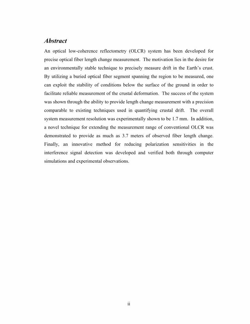
Abstract An optical low-coherence reflectometry (OLCR) system has been developed for

precise optical fiber length change measurement. The motivation lies in the desire for

an environmentally stable technique to precisely measure drift in the Earth’s crust.

By utilizing a buried optical fiber segment spanning the region to be measured, one

can exploit the stability of conditions below the surface of the ground in order to

facilitate reliable measurement of the crustal deformation. The success of the system

was shown through the ability to provide length change measurement with a precision

comparable to existing techniques used in quantifying crustal drift. The overall

system measurement resolution was experimentally shown to be 1.7 mm. In addition,

a novel technique for extending the measurement range of conventional OLCR was

demonstrated to provide as much as 3.7 meters of observed fiber length change.

Finally, an innovative method for reducing polarization sensitivities in the

interference signal detection was developed and verified both through computer

simulations and experimental observations.

iii

Table of Contents

Abstract ......................................................................................................................... ii

Table of Contents......................................................................................................... iii

Acknowledgments........................................................................................................ iv

List of Figures ............................................................................................................... v

Chapter 1: Introduction ................................................................................................ 1

1.1 Introduction to the Thesis ................................................................................... 1

1.2 Introduction to Chapters ..................................................................................... 2

Chapter 2: Principles of Optical Low-Coherence Reflectometry ................................ 3

2.1 Introduction and Operation ................................................................................. 3

2.2 Low-Coherence Source....................................................................................... 7

2.3 Dynamic Measurement Range............................................................................ 8

2.4 Sensitivity & Noise ........................................................................................... 11

2.5 Polarization Control .......................................................................................... 13

Chapter 3: Experimental Approach ........................................................................... 17

3.1 Introduction....................................................................................................... 17

3.2 OLCR Method .................................................................................................. 17

3.3 System Components & Arrangement ............................................................... 19

3.3.1 Overview.................................................................................................... 19

3.3.2 Source Arm ................................................................................................ 20

3.3.3 Test Arm .................................................................................................... 21

3.3.4 Reference Arm........................................................................................... 23

3.3.5 Receiver Arm............................................................................................. 26

Chapter 4: System Operation ..................................................................................... 30

Chapter 5: Summary of Results and Conclusions...................................................... 39

Chapter 6: Future Work ............................................................................................. 44

References................................................................................................................... 46

Appendix..................................................................................................................... 49

iv

Acknowledgments I would like to express sincere gratitude to Dr. Rongqing Hui for his guidance and

support throughout my research project. He provided me an opportunity to grow both

as a student and engineer. In addition, Dr. Hui willingly shared his knowledge and

expertise on relevant topics and gave me the freedom to explore new ideas related to

the project.

I also thank Dr. Ken Demarest and Dr. Chris Allen for their discussions and advice

provided during my time at ITTC. Their assistance offered me invaluable direction in

my research endeavors.

My appreciation also goes out to the other student research assistants working in the

Lightwave Communications Laboratory during my time working there. They all

provided a positive atmosphere and worthwhile input into my daily experimental

activities.

Finally, I thank and send congratulations out to Baio Fu for completing the system

programming and providing me with invaluable discussions regarding our combined

work on the project. His efforts enabled me to more thoroughly gather and present

my experimental results. Most importantly, he finished the remaining work on the

project, providing a complete operational system for further testing and research by

others.

v

List of Figures

2.1 Simplified OLCR Arrangement

2.2 Example of Detected Interference Signal Current

2.3 OLCR Spatial Resolution, ∆z, vs. Source Spectral Bandwidth

2.4 Extended-Range OLCR Utilizing a Pair of Retroreflectors

2.5 Recirculating Delay Arrangement for Extended-Range OLCR

2.6 OLCR System with Polarization-Diversity Receiver

2.7 Representation of the Optical Field Polarizations at the PBS

3.1 Project OLCR System Diagram

3.2 Measured EDFA Gain Block Optical Spectrum

3.3 Measured Interference Signal Spectrum with 2, 10, and 20 V Modulation

3.4 Graphical Results of Fiber Bragg Grating Pulse Delay Measurements

3.5 Polarization Angles of Combined Reflected Test and Reference Signals

4.1 Assembled Experimental OLCR System for Fiber Length Measurement

4.2 Graphical LabVIEW Routine for 1-KHz Sinusoidal Modulation Signal

4.3 Program Serial Communication Blocks and Tunable Filter Initialization

4.4 Program Delay Line Position Zero and Filter Center Wavelength Selection

4.5 Program Delay Line Movement and Position

4.6 Program Signal Measurement Process

4.7 System Graphical User Interface

5.1 Typical System Measurement Trace

5.2 Reflection Peak Data and Gaussian Curve Fit

A.1 Measured Transmittance of 1550-nm Fiber Bragg Grating

A.2 Measured Transmittance of 1553-nm Fiber Bragg Grating

A.3 Measured Transmittance of 1556-nm Fiber Bragg Grating

A.4 Measured Transmittance of 1559-nm Fiber Bragg Grating

1

Chapter 1: Introduction

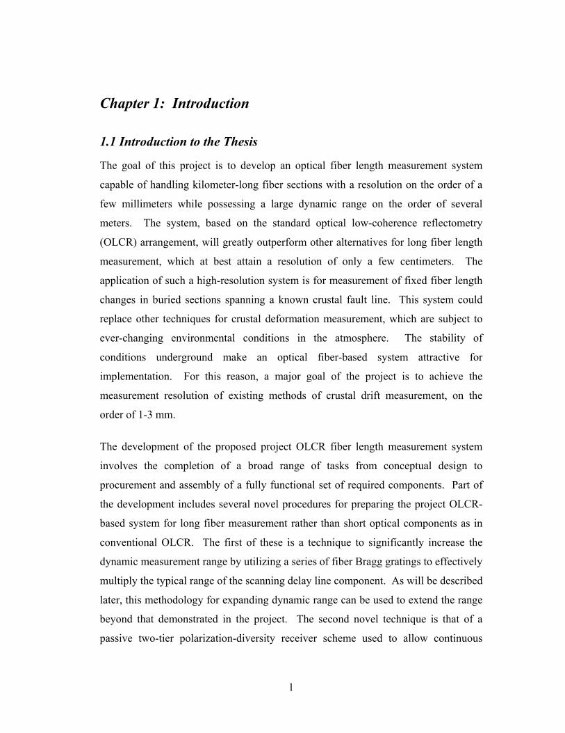
1.1 Introduction to the Thesis

The goal of this project is to develop an optical fiber length measurement system

capable of handling kilometer-long fiber sections with a resolution on the order of a

few millimeters while possessing a large dynamic range on the order of several

meters. The system, based on the standard optical low-coherence reflectometry

(OLCR) arrangement, will greatly outperform other alternatives for long fiber length

measurement, which at best attain a resolution of only a few centimeters. The

application of such a high-resolution system is for measurement of fixed fiber length

changes in buried sections spanning a known crustal fault line. This system could

replace other techniques for crustal deformation measurement, which are subject to

ever-changing environmental conditions in the atmosphere. The stability of

conditions underground make an optical fiber-based system attractive for

implementation. For this reason, a major goal of the project is to achieve the

measurement resolution of existing methods of crustal drift measurement, on the

order of 1-3 mm.

The development of the proposed project OLCR fiber length measurement system

involves the completion of a broad range of tasks from conceptual design to

procurement and assembly of a fully functional set of required components. Part of

the development includes several novel procedures for preparing the project OLCR-

based system for long fiber measurement rather than short optical components as in

conventional OLCR. The first of these is a technique to significantly increase the

dynamic measurement range by utilizing a series of fiber Bragg gratings to effectively

multiply the typical range of the scanning delay line component. As will be described

later, this methodology for expanding dynamic range can be used to extend the range

beyond that demonstrated in the project. The second novel technique is that of a

passive two-tier polarization-diversity receiver scheme used to allow continuous

2

changes in traveling signal polarizations. This scheme is important to the project

since the desired interference signal is highly dependent on polarization states of

signals traveling through the long fiber sections. The success of the two novel

techniques will be evaluated through the presentation and discussion of measurement

results for the overall project system. In addition, the results will be used to assess

the achievement of goals set out in the beginning stages of the project. This

assessment will then lend itself to a discussion on other relevant applications and/or

improvements beyond the work completed for the project.

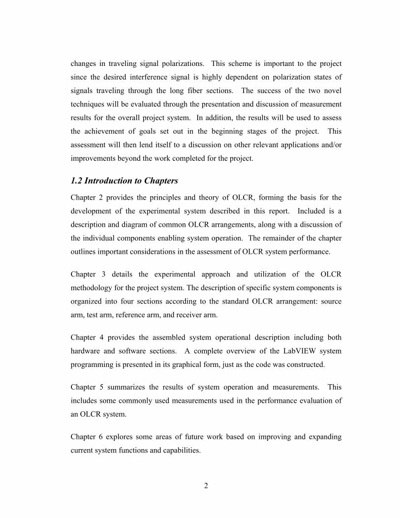
1.2 Introduction to Chapters

Chapter 2 provides the principles and theory of OLCR, forming the basis for the

development of the experimental system described in this report. Included is a

description and diagram of common OLCR arrangements, along with a discussion of

the individual components enabling system operation. The remainder of the chapter

outlines important considerations in the assessment of OLCR system performance.

Chapter 3 details the experimental approach and utilization of the OLCR

methodology for the project system. The description of specific system components is

organized into four sections according to the standard OLCR arrangement: source

arm, test arm, reference arm, and receiver arm.

Chapter 4 provides the assembled system operational description including both

hardware and software sections. A complete overview of the LabVIEW system

programming is presented in its graphical form, just as the code was constructed.

Chapter 5 summarizes the results of system operation and measurements. This

includes some commonly used measurements used in the performance evaluation of

an OLCR system.

Chapter 6 explores some areas of future work based on improving and expanding

current system functions and capabilities.

3

Chapter 2: Principles of Optical Low-Coherence

Reflectometry

2.1 Introduction and Operation

Optical low-coherence reflectometry (OLCR) was developed about 15 years ago [16],

and has since become a widely-used tool for measuring optical reflectivity as a

function of distance. OLCR has demonstrated both higher spatial resolution and

reflection sensitivity when compared to direct-detection techniques such as optical

time-domain reflectometry (OTDR) and optical frequency-domain reflectometry

(OFDR). Among other high-resolution coherent techniques, such as those based on

optical frequency scanning, OLCR offers advantages in both theoretical performance

and practical implementation [1].

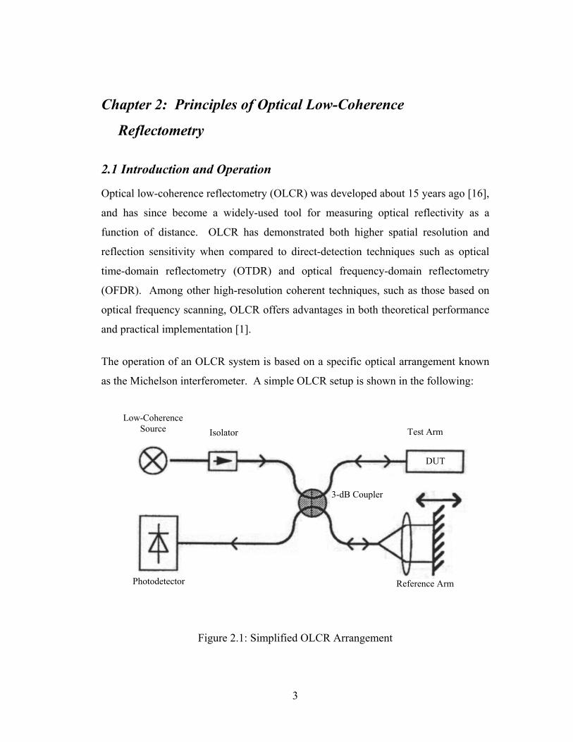
The operation of an OLCR system is based on a specific optical arrangement known

as the Michelson interferometer. A simple OLCR setup is shown in the following:

Figure 2.1: Simplified OLCR Arrangement

Photodetector

Low-Coherence Source Isolator Test Arm

3-dB Coupler

Reference Arm

DUT

4

As shown in the figure, the low-coherence source signal is divided evenly between

the reference and test arms using a 3-dB fiber coupler. The optical delay (light

propagation time) in the reference arm can then be varied by movement of the

reference mirror. The reflected signals from each arm travel back through the

coupler, where they are recombined and received at the photodiode. By nature of the

coupler, half of the reflected power will be directed back to the source where it is

attenuated by the isolator. From the arrangement shown above, an interference signal

will appear at the photodiode if the difference in optical length between the reference

and test arms is less than a coherence length. The coherence length of the system is

determined by the spectral width of the source according to the equation:

λλ∆

=n

Lc

2

where n is the refractive index of the test material, λ is the average source

wavelength, and ∆λ is the source spectral width. The incident power on the detector

leads to a photocurrent which is described by the following:

( )[ ])()(cos2 ttPPPPI DUTREFDUTREFDUTREF φφ −++= R

where R is the responsivity of the photodiode, PREF is the reflected reference signal

with optical phase of φREF (t), and PDUT is the reflected test signal with phase φDUT (t).

One assumption made in using the photocurrent expression is matched polarization

states between the reference and test reflected signals incident upon the

photodetector. This matched state maximizes the interference signal created from the

combined reflected power. Conversely, signals received at the photodiode having

orthogonal states of polarization will create no interference signal even when the

optical length of the two arms is within the coherence length, LC, of the source. The

topic of matching polarization states in OLCR measurement will be revisited in a

subsequent section of this paper.

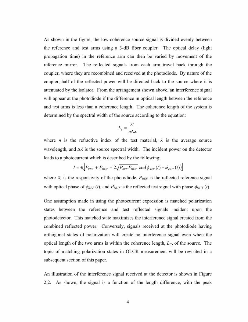
An illustration of the interference signal received at the detector is shown in Figure

2.2. As shown, the signal is a function of the length difference, with the peak

5

occurring when the optical lengths of each arm are equal. The DC value, IAVE, is a

result of the constant power, PREF and PDUT, reflected from each arm of the OLCR

arrangement. The sinusoidal wave represents the interference between the two

reflected signals received at the photodiode when the delays become equal. As the

reference arm length changes by one-half the average source wavelength, λ/2, the

sinusoidal interference signal completes one period. This is a result of the signal in

the reference arm traveling twice across the variable delay, in effect doubling the

distance.

Figure 2.2: Example of Detected Interference Signal Current

According to the photocurrent equation, when the optical length difference of the two

arms is greater than a coherence length, the phases of each path are uncorrelated,

varying randomly with respect to one another. Since the bandwidth of the

photodetector is much slower than the optical frequency at which the phase difference

varies, a constant current

will be observed at the photodiode output. However, once the length difference

decreases to less than LC, the phase term difference, φREF (t) - φDUT (t), does not

average to zero. Therefore, even though the photodetector bandwidth is unable to

z

∆z

λ/2ID

IAVE

0

6

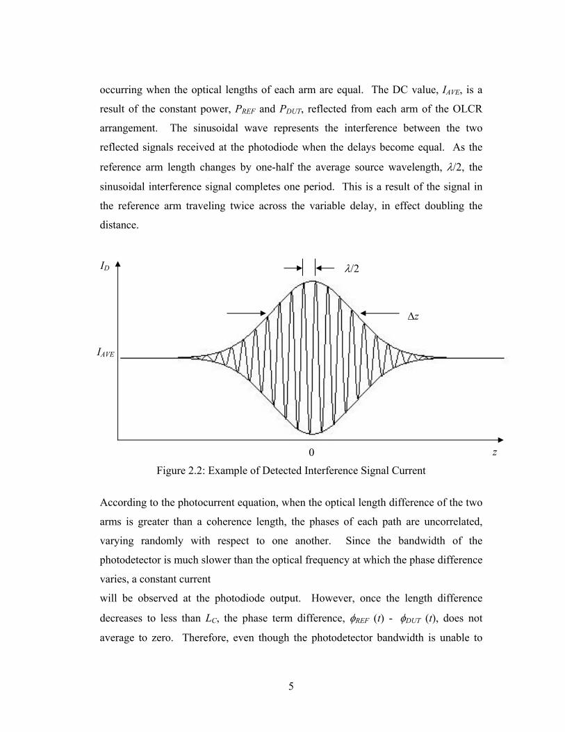
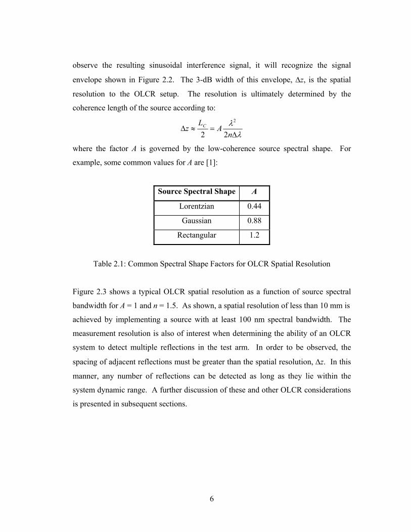
observe the resulting sinusoidal interference signal, it will recognize the signal

envelope shown in Figure 2.2. The 3-dB width of this envelope, ∆z, is the spatial

resolution to the OLCR setup. The resolution is ultimately determined by the

coherence length of the source according to:

λλ∆

=≈∆n

AL

z C

22

2

where the factor A is governed by the low-coherence source spectral shape. For

example, some common values for A are [1]:

Source Spectral Shape A

Lorentzian 0.44

Gaussian 0.88

Rectangular 1.2

Table 2.1: Common Spectral Shape Factors for OLCR Spatial Resolution

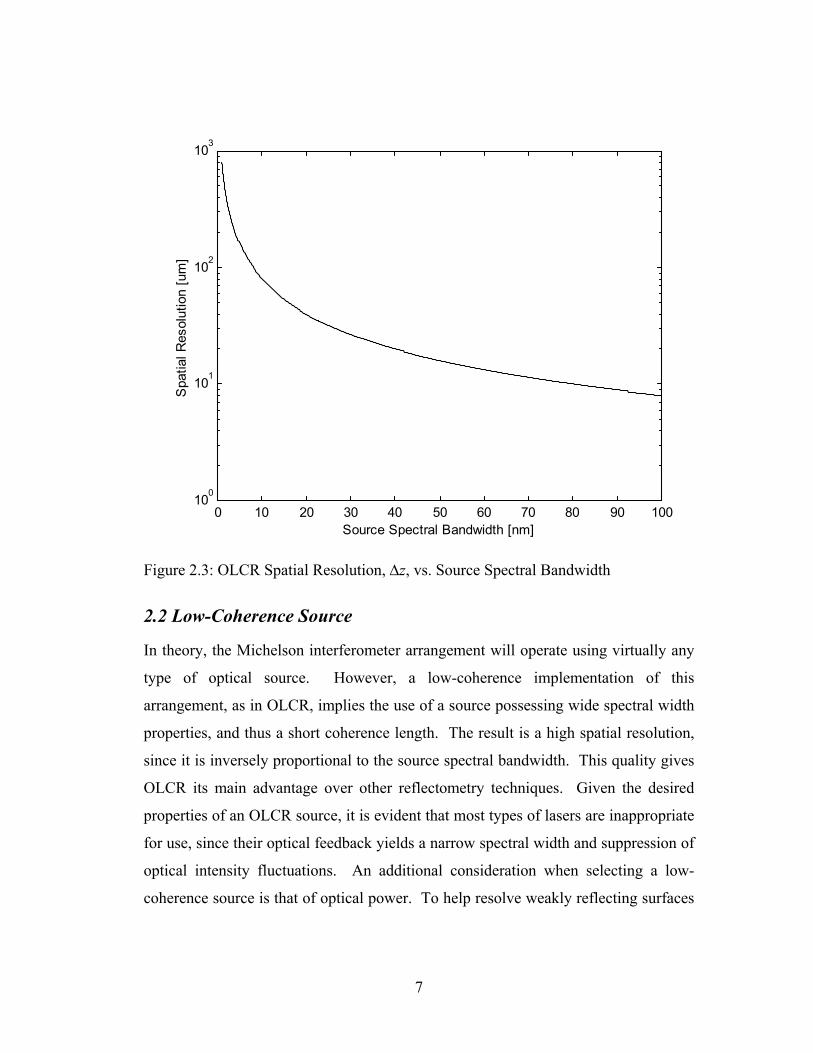
Figure 2.3 shows a typical OLCR spatial resolution as a function of source spectral

bandwidth for A = 1 and n = 1.5. As shown, a spatial resolution of less than 10 mm is

achieved by implementing a source with at least 100 nm spectral bandwidth. The

measurement resolution is also of interest when determining the ability of an OLCR

system to detect multiple reflections in the test arm. In order to be observed, the

spacing of adjacent reflections must be greater than the spatial resolution, ∆z. In this

manner, any number of reflections can be detected as long as they lie within the

system dynamic range. A further discussion of these and other OLCR considerations

is presented in subsequent sections.

7

0 10 20 30 40 50 60 70 80 90 100100

101

102

103

Source Spectral Bandwidth [nm]

Spa

tial R

esol

utio

n [u

m]

Figure 2.3: OLCR Spatial Resolution, ∆z, vs. Source Spectral Bandwidth

2.2 Low-Coherence Source

In theory, the Michelson interferometer arrangement will operate using virtually any

type of optical source. However, a low-coherence implementation of this

arrangement, as in OLCR, implies the use of a source possessing wide spectral width

properties, and thus a short coherence length. The result is a high spatial resolution,

since it is inversely proportional to the source spectral bandwidth. This quality gives

OLCR its main advantage over other reflectometry techniques. Given the desired

properties of an OLCR source, it is evident that most types of lasers are inappropriate

for use, since their optical feedback yields a narrow spectral width and suppression of

optical intensity fluctuations. An additional consideration when selecting a low-

coherence source is that of optical power. To help resolve weakly reflecting surfaces

8

in the test arm, higher incident power typically results in a stronger interference

signal. Therefore, an increase in overall sensitivity of the OLCR system is observed.

The most common sources used in OLCR today possess a combination of spectral

bandwidth and optical power. The first is an edge-emitting light emitting diode

(EELED), which typically outputs approximately 100 µW of power with a spectral

width of 50 nm. This combination provides an approximate 16 µm resolution in fiber

at 1550 nm and relatively good measurement sensitivity with respect to the low-cost

nature of EELEDs. One possible problem with the use of a standard EELED is the

introduction of sidelobes to the OLCR measurement trace. The phenomenon of

sidelobes will be discussed in a later section of the paper.

Another commonly used source in OLCR is the erbium-doped fiber amplifier

(EDFA). The amplified spontaneous emission (ASE) output of the EDFA can

provide in excess of 10 mW optical power with a spectral width of approximately 20

nm. This high output power makes the EDFA a good choice over the EELED when

greater reflection sensitivity is desired. In addition, the operation of the EDFA leads

to better suppression of measurement sidelobes. The few disadvantages in using an

EDFA are the decrease in resolution, due to a more narrow spectral width, and the

significantly higher cost when compared to the EELED. These considerations, along

with the desired measurement sensitivity, are usually the basis for the final decision

of which low-coherence source one chooses.

2.3 Dynamic Measurement Range

The measurement range of an OLCR system is the maximum distance over which

reflections in the test arm can be detected. This range is directly proportional to the

maximum scanning distance (delay) available in the reference arm. The variable

optical delay is commonly provided by a movable mirror or fiber scanning delay line.

For many fiber components used as the DUT in the test arm, the normal dynamic

range of several tens of centimeters is adequate. However, there is continued

9

development in the area of expanded OLCR measurement range to enable enhanced

system performance and new applications. This area is in fact the focus of this paper

and others working to expand OLCR system range performance.

One of the most basic ways to increase OLCR measurement range is to combine

separate successive variable delay scans, adding additional fiber length to the test or

reference arms between each scan. In its simplest implementation, this method would

involve sequentially adding sections of fiber to one of the arms, each piece being

equivalent to the maximum optical distance of the reference arm variable delay. The

disadvantage of this technique is the necessity to physically attach sections of fiber to

the system between delay scans. However, this simple idea is a practical one and

provides the basis for developing the extended-range OLCR system outlined and

tested further in this paper. As will be shown, the basic idea was improved by

incorporating a novel technique for adding fiber sections without physically attaching

them between each reference arm scan.

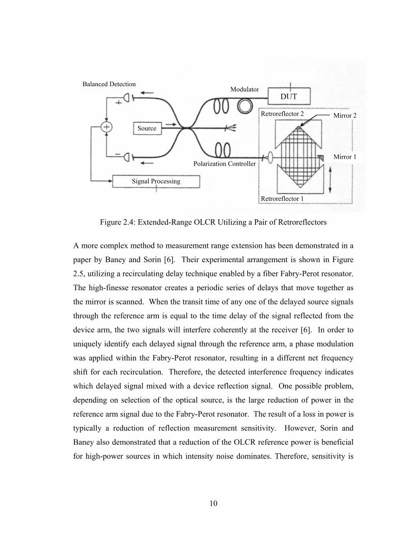
Another method for expanding OLCR dynamic range was demonstrated by Takada et

al [12]. This technique involves folding the optical path between the fiber and

scanning mirror, effectively increasing the scanning distance in the reference arm by

a factor of 10. A diagram of the experimental system setup used by Takada is shown

in Figure 2.4. As shown in the arrangement, a pair of retroreflectors provides the

means of dynamic range extension by increasing the air path in which the reference

arm signal travels. As evident from the arrangement, one disadvantage of this

technique is an increase in the air path of the reference arm leads to higher differential

dispersion with the test arm resulting in a relative degradation of spatial resolution.

10

Figure 2.4: Extended-Range OLCR Utilizing a Pair of Retroreflectors

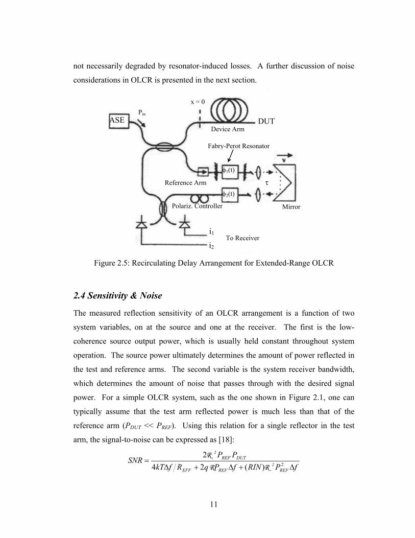
A more complex method to measurement range extension has been demonstrated in a

paper by Baney and Sorin [6]. Their experimental arrangement is shown in Figure

2.5, utilizing a recirculating delay technique enabled by a fiber Fabry-Perot resonator.

The high-finesse resonator creates a periodic series of delays that move together as

the mirror is scanned. When the transit time of any one of the delayed source signals

through the reference arm is equal to the time delay of the signal reflected from the

device arm, the two signals will interfere coherently at the receiver [6]. In order to

uniquely identify each delayed signal through the reference arm, a phase modulation

was applied within the Fabry-Perot resonator, resulting in a different net frequency

shift for each recirculation. Therefore, the detected interference frequency indicates

which delayed signal mixed with a device reflection signal. One possible problem,

depending on selection of the optical source, is the large reduction of power in the

reference arm signal due to the Fabry-Perot resonator. The result of a loss in power is

typically a reduction of reflection measurement sensitivity. However, Sorin and

Baney also demonstrated that a reduction of the OLCR reference power is beneficial

for high-power sources in which intensity noise dominates. Therefore, sensitivity is

DUT

Mirror 1

Mirror 2Retroreflector 2

Retroreflector 1

Source

Modulator

Polarization Controller

Signal Processing

Balanced Detection

11

not necessarily degraded by resonator-induced losses. A further discussion of noise

considerations in OLCR is presented in the next section.

Figure 2.5: Recirculating Delay Arrangement for Extended-Range OLCR

2.4 Sensitivity & Noise

The measured reflection sensitivity of an OLCR arrangement is a function of two

system variables, on at the source and one at the receiver. The first is the low-

coherence source output power, which is usually held constant throughout system

operation. The source power ultimately determines the amount of power reflected in

the test and reference arms. The second variable is the system receiver bandwidth,

which determines the amount of noise that passes through with the desired signal

power. For a simple OLCR system, such as the one shown in Figure 2.1, one can

typically assume that the test arm reflected power is much less than that of the

reference arm (PDUT << PREF). Using this relation for a single reflector in the test

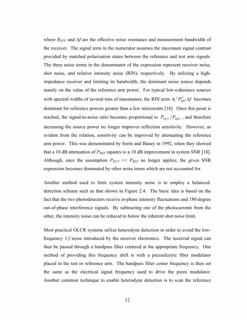
arm, the signal-to-noise can be expressed as [18]:

fPRINfPqRfkTPP

SNRREFREFEFF

DUTREF

∆+∆+∆= 2)(24

22

2

RRR

Mirror

τ

DUTDevice Arm

x = 0

Reference Arm

Pin ASE

i1

i2To Receiver

Polariz. Controller

φ1(t)

φ2(t)

Fabry-Perot Resonator

12

where REFF and ∆f are the effective noise resistance and measurement bandwidth of

the receiver. The signal term in the numerator assumes the maximum signal contrast

provided by matched polarization states between the reference and test arm signals.

The three noise terms in the denominator of the expression represent receiver noise,

shot noise, and relative intensity noise (RIN), respectively. By utilizing a high-

impedance receiver and limiting its bandwidth, the dominant noise source depends

mainly on the value of the reference arm power. For typical low-coherence sources

with spectral widths of several tens of nanometers, the RIN term fPREF ∆22R becomes

dominant for reference powers greater than a few microwatts [18]. Once this point is

reached, the signal-to-noise ratio becomes proportional to REFDUT PP , and therefore

increasing the source power no longer improves reflection sensitivity. However, as

evident from the relation, sensitivity can be improved by attenuating the reference

arm power. This was demonstrated by Sorin and Baney in 1992, when they showed

that a 10 dB attenuation of PREF equates to a 10 dB improvement in system SNR [18].

Although, once the assumption PDUT << PREF no longer applies, the given SNR

expression becomes dominated by other noise terms which are not accounted for.

Another method used to limit system intensity noise is to employ a balanced-

detection scheme such as that shown in Figure 2.4. The basic idea is based on the

fact that the two photodetectors receive in-phase intensity fluctuations and 180-degree

out-of-phase interference signals. By subtracting one of the photocurrents from the

other, the intensity noise can be reduced to below the inherent shot noise limit.

Most practical OLCR systems utilize heterodyne detection in order to avoid the low-

frequency 1/f noise introduced by the receiver electronics. The received signal can

then be passed through a bandpass filter centered at the appropriate frequency. One

method of providing this frequency shift is with a piezoelectric fiber modulator

placed in the test or reference arm. The bandpass filter center frequency is then set

the same as the electrical signal frequency used to drive the piezo modulator.

Another common technique to enable heterodyne detection is to scan the reference

13

mirror at a constant velocity, vm. The resulting center frequency for the receiver

bandpass filter is given by:

λmv

f2

=

where λ is the low-coherence source average wavelength. By utilizing all of the

discussed techniques for minimizing OLCR receiver noise, reflection sensitivities

within just a few dB of the shot noise limit have been demonstrated.

In addition to the received interference signal and its associated noise, unwanted

signals can also be detected at the receiver if multiple unexpected reflections occur in

the system. These signals show up as sidelobes to the desired signal in the

measurement trace. These sidelobes result from double reflections within weak

etalons anywhere in the optical path. One common source of sidelobes, as discussed

earlier, is facet reflections within the source such as an EELED. Since this etalon is

present in the source arm, symmetrical sidelobes will occur around the primary signal

since the unwanted signal travels through both the test and reference arms.

Alternatively, if the weak etalon exists in either of the reflective arms, the result is a

single sidelobe next to the primary signal. For a stray signal in the reference arm the

sidelobe appears to the left of the primary, and one from the test arm results in a

sidelobe to right, with increasing delay distance represented from left to right. These

three different scenarios enable one to more easily determine the source of

measurement sidelobes.

2.5 Polarization Control

As indicated earlier, optimum OLCR performance is achieved when the polarization

is matched between signals reflected from the test and reference arms. Regardless of

the unpolarized nature of low-coherence sources, one must incorporate polarization

matching techniques in virtually every OLCR system in order to ensure an

interference signal at the receiver. The reason is that the source light is considered

unpolarized in a time-averaged sense only, so at any instantaneous time the light has a

14

specific polarization state. One is interested in this state because as the signal splits

and travels down the test and reference arms, it is reflected and recombined in the

receiver arm. Therefore, the reflected signals mix and create an interference pattern

not only if their optical time delays are within a coherence time, but also if their

polarization states are not orthogonal to one another. The problem of matched

polarization arises from the fact that the split source signal travels along two separate

paths in the test and reference arms, each of which alters the polarization state of their

signals independently. As a result, the states of polarization of the two signals, upon

recombining in the receiver arm, quite commonly will not be matched to provide

optimum measurement sensitivity.

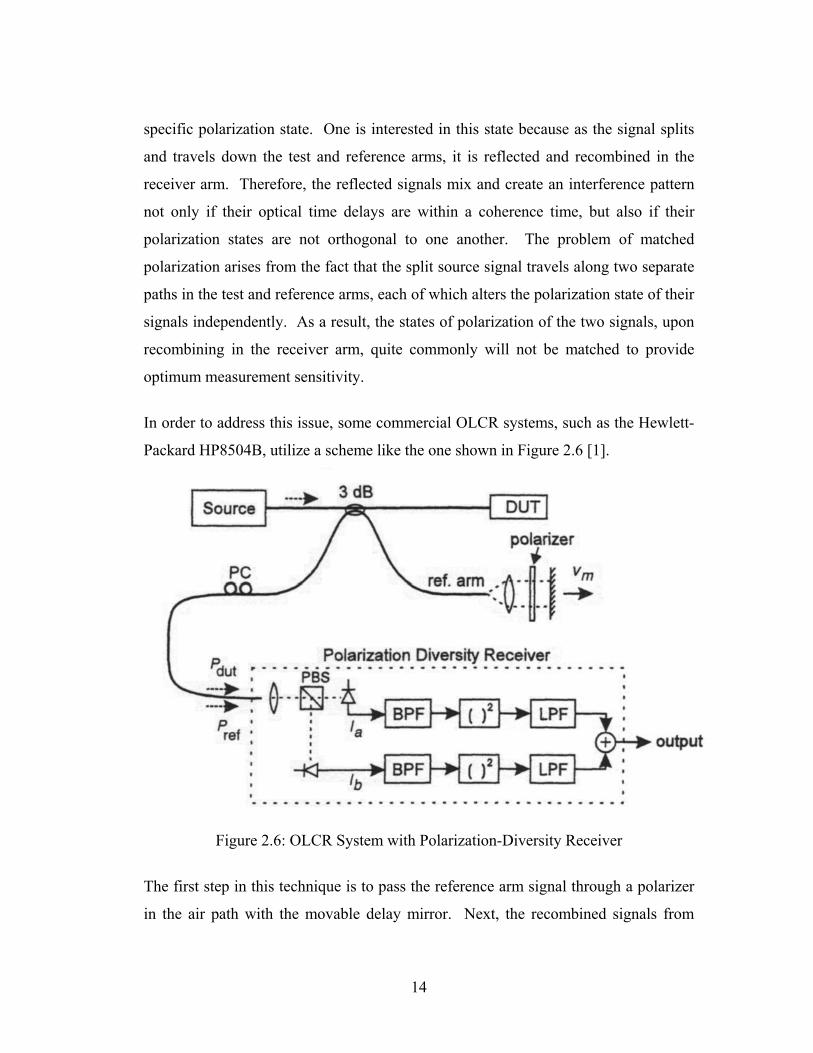
In order to address this issue, some commercial OLCR systems, such as the Hewlett-

Packard HP8504B, utilize a scheme like the one shown in Figure 2.6 [1].

Figure 2.6: OLCR System with Polarization-Diversity Receiver

The first step in this technique is to pass the reference arm signal through a polarizer

in the air path with the movable delay mirror. Next, the recombined signals from

15

both arms travel through a polarization controller (PC), which is adjusted to alter the

orientation of the incoming polarization of the signals approaching the receiver.

Upon entering the polarization-diversity receiver, the incoming light is passed

through a polarizing beam splitter (PBS), then on to two individual photodetectors.

The incident power on each of the photodiodes is divided equally by further

adjustment of the PC, which aligns the polarized reference signal with the PBS.

Similar to previous discussions, this scheme assumes the reflected test arm power is

much less than that of reference arm, PDUT << PREF. This assumption enables one to

properly align the polarized reference signal with the PBS by simply dividing the

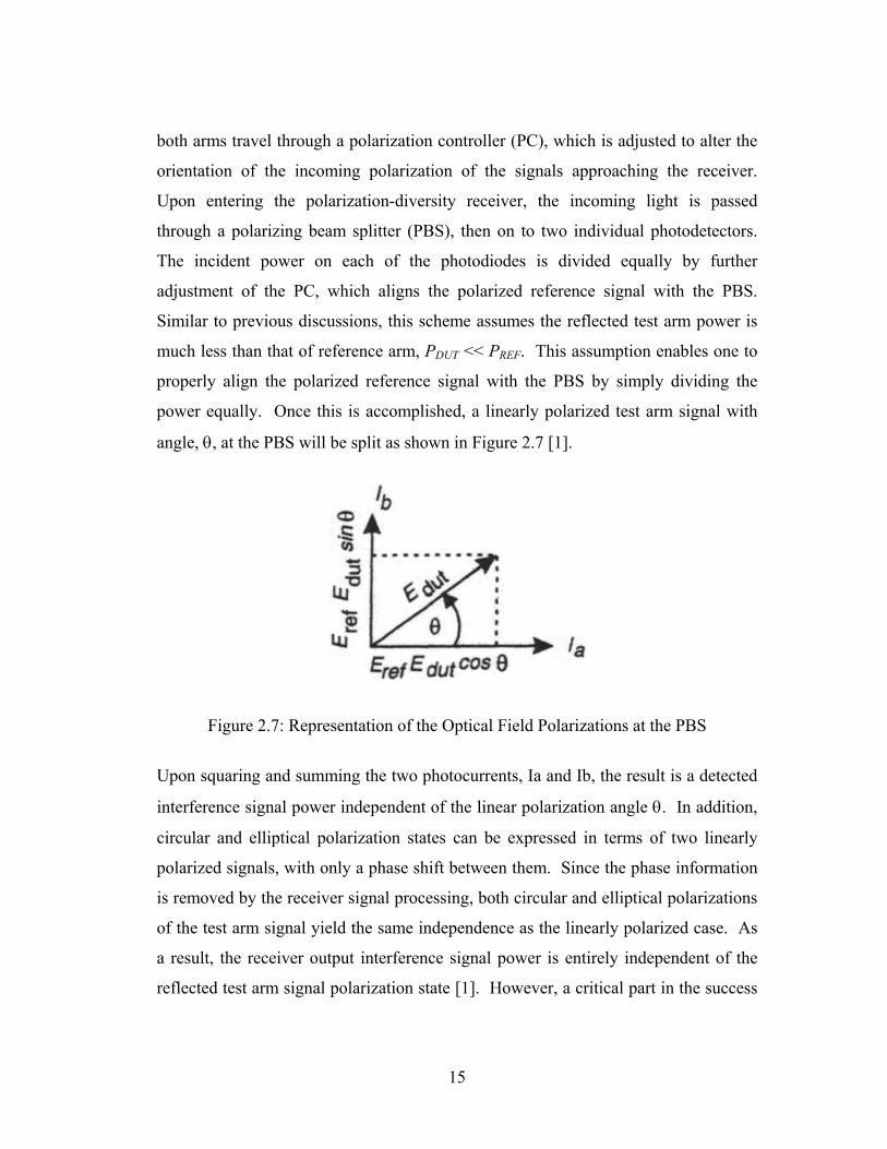
power equally. Once this is accomplished, a linearly polarized test arm signal with

angle, θ, at the PBS will be split as shown in Figure 2.7 [1].

Figure 2.7: Representation of the Optical Field Polarizations at the PBS

Upon squaring and summing the two photocurrents, Ia and Ib, the result is a detected

interference signal power independent of the linear polarization angle θ. In addition,

circular and elliptical polarization states can be expressed in terms of two linearly

polarized signals, with only a phase shift between them. Since the phase information

is removed by the receiver signal processing, both circular and elliptical polarizations

of the test arm signal yield the same independence as the linearly polarized case. As

a result, the receiver output interference signal power is entirely independent of the

reflected test arm signal polarization state [1]. However, a critical part in the success

16

of this type of OLCR system measurement is ensuring that the reference arm signal

polarization state does not change. This can be accomplished by preventing the

reference arm fiber from being disturbed or subjected to temperature changes in the

surrounding. In doing so, highly repeatable results can be achieved.

17

Chapter 3: Experimental Approach

3.1 Introduction

The motivation behind the OLCR measurement system developed in this project lies

in the desire for an environmentally stable technique to precisely measure drift in the

Earth’s crust. By utilizing a buried optical fiber segment spanning the region to be

measured, one can exploit the stability of conditions below the surface of the ground

in order to facilitate reliable measurement of the crustal deformation. The final

consideration, as explored in this project, is to provide measurement of this buried

fiber length with a precision comparable to existing techniques used in quantifying

crustal drift. Currently, those existing techniques achieve typically a 1-3 millimeter

resolution over a 10 km span. However, a major concern for these current methods is

the impact of environmental factors, since they all are susceptible to frequent changes

in atmospheric conditions. The goal for this project, therefore, is to implement a fiber

length measurement scheme capable of meeting the criteria set forth by existing

methods, and at the same time utilize a stable media over which to operate.

3.2 OLCR Method

As evident from the previous chapter regarding the principles of OLCR, the main

focus of conventional systems is to detect internal reflections within commonly

utilized optical and fiber-optic components. To fit this need, most commercially

available OLCR systems provide a high spatial resolution and relatively small

dynamic range, since even the largest optical components are usually no more than

several tens of centimeters in length. In addition, these systems provide only test arm

polarization control, which once adjusted, cannot adapt to changes in the signal

polarization of the reference arm. Again, this type of approach is suitable for

component reflection measurements, since the reference arm length can be kept short

and stable, effectively minimizing polarization changes during measurement.

18

The experimental system developed and described in the following section seeks to

use the basic principles of OLCR and apply them to high resolution, long fiber length

measurements rather than short optical component measurements. In doing so, it is

necessary to alter some of the aspects of conventional OLCR in order to optimize its

use for this purpose. To fit the intended use, the main areas of focus in this project’s

experimental OLCR system become two-fold. The first aspect is focused on

expanding the dynamic range of the system to several meters, as opposed to several

tens of centimeters, which is currently the typical range for commercial OLCR

systems. As a result, our approach sacrifices measurement resolution. However, the

goal for the theoretical resolution of our system, on the order of one millimeter,

remains far better than that of other techniques used for long fiber length

measurement. Once such commonly used approach is optical-time domain

reflectometry (OTDR), which utilizes short optical pulses for its fiber length

measurements. In commercially available OTDR systems, the dynamic range is

typically much larger than necessary for our purpose, however, the spatial resolution

is on the order of several tens of meters. Limitations in currently available

components do not enable OTDR measurements to reach the desired high resolution

of our system. As a result, the choice was made to develop an OLCR-based system

with an expanded dynamic range of several meters and a measurement resolution in

the millimeter range.

Based on the development of an OLCR system, the second area of focus is the aspect

of a polarization diversity receiver, which allows changes to both the reference and

test arm signal polarizations during measurement. This is desired since long fiber

sections tend to impart constantly changing effects on the polarization of a traveling

signal. Current commercial techniques, based on a constant reference arm signal

polarization state, are not sufficient for the intended use here. Furthermore, the

currently-used OLCR polarization diversity schemes assume a weakly reflected

signal from the test arm. In the case of this project, the test arm will terminate with a

highly reflective surface which creates a reflected signal closely matching in power to

19

that traveling from the reference arm. This project utilizes the similarities in power

between the two arms to develop a novel, passive polarization diversity scheme

which does not require initial calibration with respect to either the test or reference

arm. In addition, the polarization state of either arm can vary arbitrarily without loss

of the interference signal. The implications of this novel scheme on the received

interference signal power will be explored later in this discussion. The remaining

aspects of the system developed in this project closely resemble those of conventional

OLCR, as will be evident in the experimental component descriptions in the next

section.

3.3 System Components & Arrangement

3.3.1 Overview

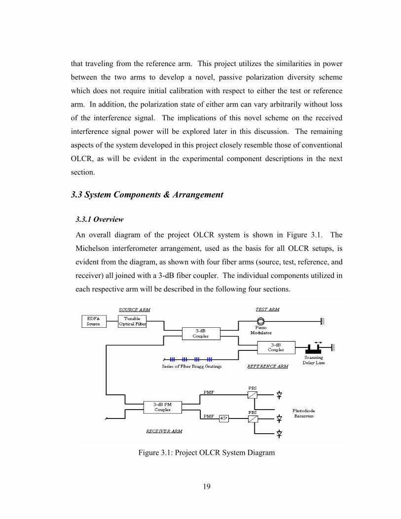
An overall diagram of the project OLCR system is shown in Figure 3.1. The

Michelson interferometer arrangement, used as the basis for all OLCR setups, is

evident from the diagram, as shown with four fiber arms (source, test, reference, and

receiver) all joined with a 3-dB fiber coupler. The individual components utilized in

each respective arm will be described in the following four sections.

Figure 3.1: Project OLCR System Diagram

20

3.3.2 Source Arm

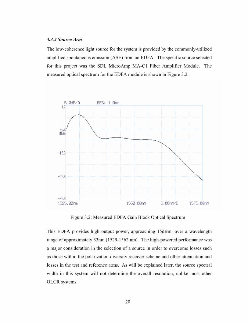
The low-coherence light source for the system is provided by the commonly-utilized

amplified spontaneous emission (ASE) from an EDFA. The specific source selected

for this project was the SDL MicroAmp MA-C1 Fiber Amplifier Module. The

measured optical spectrum for the EDFA module is shown in Figure 3.2.

Figure 3.2: Measured EDFA Gain Block Optical Spectrum

This EDFA provides high output power, approaching 15dBm, over a wavelength

range of approximately 33nm (1529-1562 nm). The high-powered performance was

a major consideration in the selection of a source in order to overcome losses such

as those within the polarization-diversity receiver scheme and other attenuation and

losses in the test and reference arms. As will be explained later, the source spectral

width in this system will not determine the overall resolution, unlike most other

OLCR systems.

21

The current supply and temperature control for the EDFA gain block are provided

externally through the use of two devices manufactured by Wavelength Electronics.

The first is the MPL-250 Laser Driver module supplying up to 250 mA of current to

the EDFA pump laser. The optical spectrum shown in Figure 3.2 was obtained

using 150-175 mA of drive current. The second external module is the MPT-2500

2.5-A Temperature Controller which provides current to the Peltier thermoelectric

cooling device within the EDFA compartment. The temperature of the pump laser

diode is controlled according to the measured resistance of a thermistor mounted

near the laser. These two externally mounted components enable the use of the

extremely compact EDFA module utilized in the system enclosure.

A final component used in the source arm is an electronically-tunable optical filter.

Specifically, an OZ Optics TF-100-MC Motor-Driven Tunable Filter was designed

with a 1.5-nm filter bandwidth and RS-232 serial communications control interface.

This unit was selected for its computer control capabilities and low insertion and

polarization-dependent losses, which measured approximately 3 dB and 0.2 dB

respectively. This component is not normally found in a conventional OLCR

system since it narrows the spectral width of the source, thus decreasing

measurement resolution. However, in this specific arrangement the tunable filter

enables a novel technique for system dynamic range extension that will be described

in further detail in the discussion of the reference arm components. In addition, this

project does not require the extremely high resolution normally provided by OLCR.

The overall system resolution, in this case, is mainly determined not by the source

spectral width, but the filter bandwidth of 1.5 nm. Based on Figure 2.3, this width

should easily provide the target goal of 1-2 mm system resolution.

3.3.3 Test Arm

As shown in the system diagram, the test arm consists of a fiber piezo modulator

connected to a long fiber section with a total reflecting termination at the far end.

The long terminated fiber, on the order of a kilometer in length, replaces the Device-

22

Under-Test, normally no more than several centimeters, in conventional OLCR

applications. This represents on of the major changes from typical OLCR

components in this project. As described earlier, changes in the length of this long

fiber are what the project ultimately seeks to measure. The piezo modulator is

utilized to heterodyne the interference signal, shifting the spectrum away from DC

and thus reducing the low-frequency noise introduced in the receiver electronics.

The modulator component consists of a cylindrical piezoelectric device

approximately 5 cm in diameter with a 1-meter fiber patch cable wrapped tightly

around the perimeter. By biasing the piezo device with a sinusoidal voltage, small

periodic changes in the cylinder diameter induce a periodic modulation of the length

of the tightly wrapped fiber. The result is a sinusoidal phase (length) modulation in

the test arm signal, thus ultimately providing a heterodyned OLCR interference

signal at the output of the receiver. In addition, the interference signal frequency

spectrum has a major component at the piezo bias frequency and, since the

modulating device is not perfectly efficient, at the next several harmonic

frequencies. The piezoelectric device bias frequency determination was made

mainly by system trial-and-error, adjusting the sinusoidal source while monitoring

the received interference signal. It was found that a biasing frequency beyond

approximately 10 kHz exceeded the effective response of the modulating device. In

addition, a frequency above several kilohertz produced an audible vibration in the

piezoelectric device. With these considerations, the decision was made to use 1-

kHz as the frequency for the bias voltage. Next, the determination of bias signal

amplitude was made through observations of its effect on the interference signal

spectrum. The results of three tested bias signal voltages (1, 5, and 10 V) on the

received interference spectrum are shown in Figure 3.3.

23

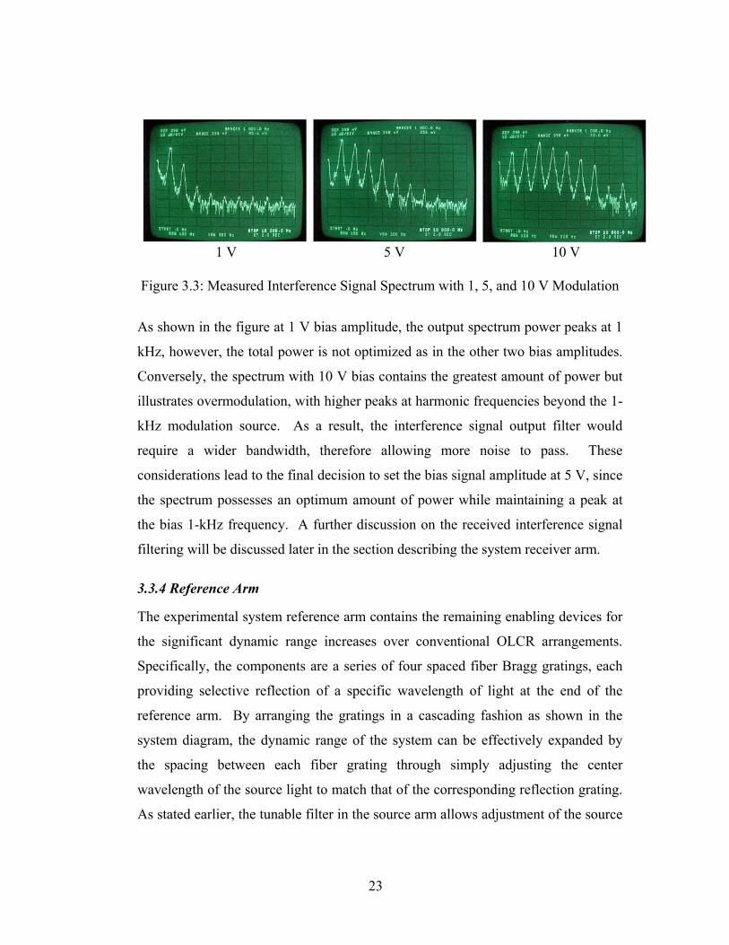
Figure 3.3: Measured Interference Signal Spectrum with 1, 5, and 10 V Modulation

As shown in the figure at 1 V bias amplitude, the output spectrum power peaks at 1

kHz, however, the total power is not optimized as in the other two bias amplitudes.

Conversely, the spectrum with 10 V bias contains the greatest amount of power but

illustrates overmodulation, with higher peaks at harmonic frequencies beyond the 1-

kHz modulation source. As a result, the interference signal output filter would

require a wider bandwidth, therefore allowing more noise to pass. These

considerations lead to the final decision to set the bias signal amplitude at 5 V, since

the spectrum possesses an optimum amount of power while maintaining a peak at

the bias 1-kHz frequency. A further discussion on the received interference signal

filtering will be discussed later in the section describing the system receiver arm.

3.3.4 Reference Arm

The experimental system reference arm contains the remaining enabling devices for

the significant dynamic range increases over conventional OLCR arrangements.

Specifically, the components are a series of four spaced fiber Bragg gratings, each

providing selective reflection of a specific wavelength of light at the end of the

reference arm. By arranging the gratings in a cascading fashion as shown in the

system diagram, the dynamic range of the system can be effectively expanded by

the spacing between each fiber grating through simply adjusting the center

wavelength of the source light to match that of the corresponding reflection grating.

As stated earlier, the tunable filter in the source arm allows adjustment of the source

1 V 5 V 10 V

24

signal output center wavelength with a constant spectral width of 1.5 nm.

Additionally, the transmissivity of each of the four gratings has a spectral notch at

wavelengths of 1550, 1553, 1556, and 1559 nm. Together, these components

enable automatic system operation at the four respective wavelengths, each

expanding the effective dynamic range by the length of the spacing between each

grating. The fiber Bragg gratings utilized for this project were manufactured by O/E

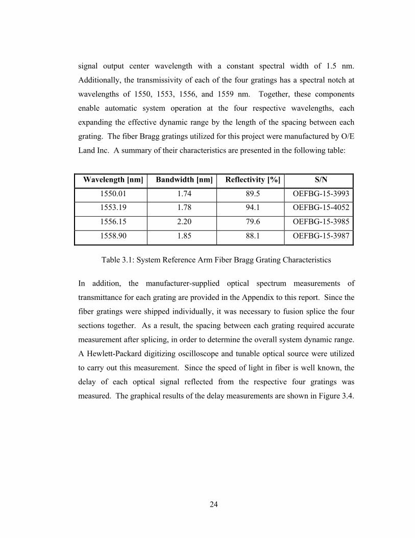
Land Inc. A summary of their characteristics are presented in the following table:

Wavelength [nm] Bandwidth [nm] Reflectivity [%] S/N

1550.01 1.74 89.5 OEFBG-15-3993

1553.19 1.78 94.1 OEFBG-15-4052

1556.15 2.20 79.6 OEFBG-15-3985

1558.90 1.85 88.1 OEFBG-15-3987

Table 3.1: System Reference Arm Fiber Bragg Grating Characteristics

In addition, the manufacturer-supplied optical spectrum measurements of

transmittance for each grating are provided in the Appendix to this report. Since the

fiber gratings were shipped individually, it was necessary to fusion splice the four

sections together. As a result, the spacing between each grating required accurate

measurement after splicing, in order to determine the overall system dynamic range.

A Hewlett-Packard digitizing oscilloscope and tunable optical source were utilized

to carry out this measurement. Since the speed of light in fiber is well known, the

delay of each optical signal reflected from the respective four gratings was

measured. The graphical results of the delay measurements are shown in Figure 3.4.

25

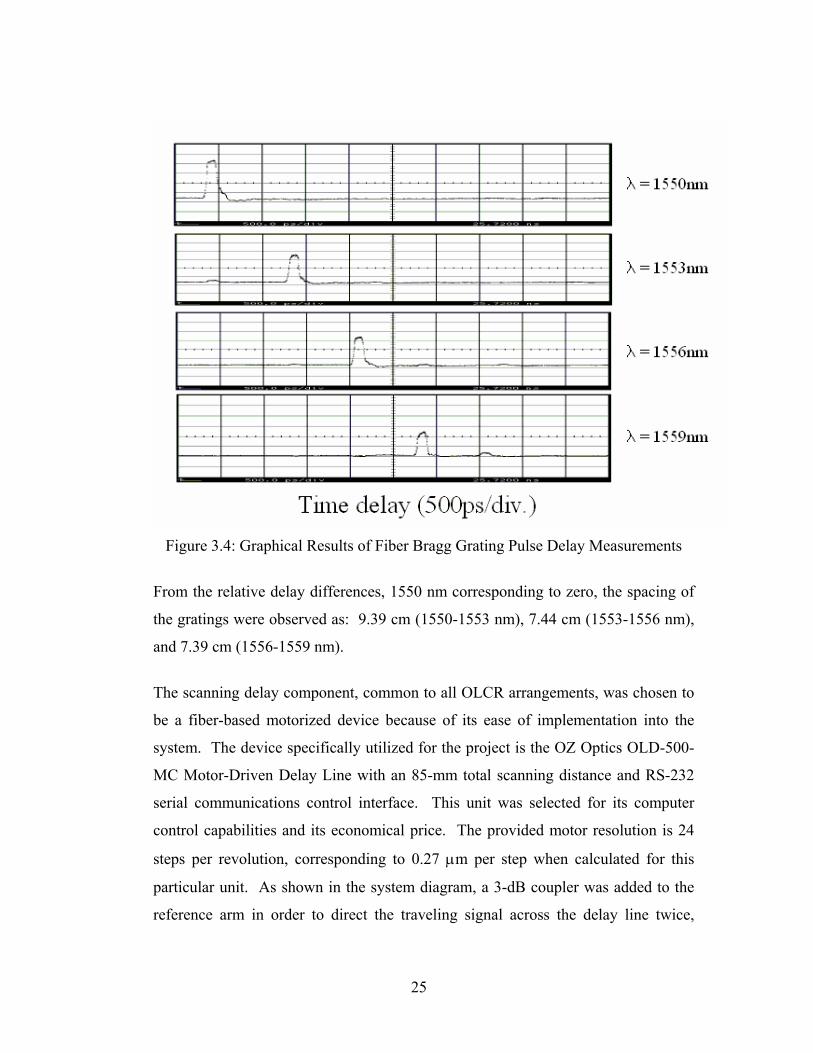
Figure 3.4: Graphical Results of Fiber Bragg Grating Pulse Delay Measurements

From the relative delay differences, 1550 nm corresponding to zero, the spacing of

the gratings were observed as: 9.39 cm (1550-1553 nm), 7.44 cm (1553-1556 nm),

and 7.39 cm (1556-1559 nm).

The scanning delay component, common to all OLCR arrangements, was chosen to

be a fiber-based motorized device because of its ease of implementation into the

system. The device specifically utilized for the project is the OZ Optics OLD-500-

MC Motor-Driven Delay Line with an 85-mm total scanning distance and RS-232

serial communications control interface. This unit was selected for its computer

control capabilities and its economical price. The provided motor resolution is 24

steps per revolution, corresponding to 0.27 µm per step when calculated for this

particular unit. As shown in the system diagram, a 3-dB coupler was added to the

reference arm in order to direct the traveling signal across the delay line twice,

26

effectively doubling the available scanning distance from 85 mm to 170 mm. Since

the delay line must scan the length between each fiber grating, this increased

distance is necessary to reach the 9.4 cm space between the first two gratings. This

double-pass arrangement in the reference arm also effectively reduces the unit

resolution by half to 0.54 µm, however, this change will not significantly degrade

measurement performance since the system resolution is expected to be

approximately 1.5 mm. With the scanning delay unit now defined, the overall

system dynamic range can be figured by adding the total length between fiber

gratings and the available scanning distance beyond the last grating to yield an

overall value of more than 41 cm. More importantly, the number of gratings can be

increased up to the available bandwidth of the source in order to easily achieve a

dynamic range of over 1 m in length. Furthermore, this range could be increased

additionally by maximizing the spacing between each grating up to the available

scanning delay distance.

3.3.5 Receiver Arm

The final component descriptions come from the receiver arm where the reflected

signals from the test and reference arm recombine and mix to create the desired

interference signal. As stated earlier, the main goal of the device arrangement in

this arm is to provide a passive polarization-diversity receiver that does not require

initial calibration to either of the reflective arms. The first step in achieving this is

to send the incoming signals through a 3-dB polarization-maintaining (PM) coupler,

as shown in the system diagram. The coupler essentially divides and freezes the

state of the exiting signals to a fixed polarization. A representation of the

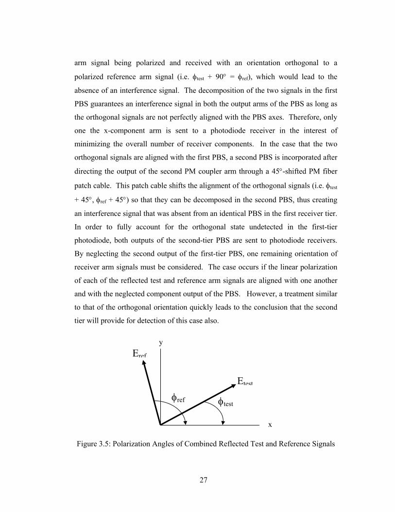
polarization angles between the traveling polarized signals is shown in Figure 3.5.

Half of the incoming reference arm signal power is then sent down one of two PM

fibers where it is divided in a polarization beam splitter (PBS). This device

essentially decomposes an arbitrarily polarized signal into orthogonal components

(represented by X and Y in Figure 3.5) and sends each to one of two output arms.

This first tier of the polarization diversity receiver protects against a reflected test

27

arm signal being polarized and received with an orientation orthogonal to a

polarized reference arm signal (i.e. φtest + 90° = φref), which would lead to the

absence of an interference signal. The decomposition of the two signals in the first

PBS guarantees an interference signal in both the output arms of the PBS as long as

the orthogonal signals are not perfectly aligned with the PBS axes. Therefore, only

one the x-component arm is sent to a photodiode receiver in the interest of

minimizing the overall number of receiver components. In the case that the two

orthogonal signals are aligned with the first PBS, a second PBS is incorporated after

directing the output of the second PM coupler arm through a 45°-shifted PM fiber

patch cable. This patch cable shifts the alignment of the orthogonal signals (i.e. φtest

+ 45°, φref + 45°) so that they can be decomposed in the second PBS, thus creating

an interference signal that was absent from an identical PBS in the first receiver tier.

In order to fully account for the orthogonal state undetected in the first-tier

photodiode, both outputs of the second-tier PBS are sent to photodiode receivers.

By neglecting the second output of the first-tier PBS, one remaining orientation of

receiver arm signals must be considered. The case occurs if the linear polarization

of each of the reflected test and reference arm signals are aligned with one another

and with the neglected component output of the PBS. However, a treatment similar

to that of the orthogonal orientation quickly leads to the conclusion that the second

tier will provide for detection of this case also.

Figure 3.5: Polarization Angles of Combined Reflected Test and Reference Signals

φtest φref

x

y Eref

Etest

28

The three optical receivers chosen for the system were manufactured by Terahertz

Technology Inc. Each of the three boards contain an InGaAs detector and

associated FC optical connection. Also, included is the necessary power

connections and associated electronic components needed to carry out he

optical/electrical conversion. Since the detected interference signal is modulated at

1 KHz by the piezoelectric device in the test arm, the receiver electronics low-pass

cutoff frequency was selected as 10 KHz so that the major signal harmonic

components are converted, as shown in Figure 3.3 at 10V modulation amplitude,

while still filtering out the undesired high frequency noise above 10-KHz. The

receiver board electronics were further modified in the lab to provide a 400-Hz

high-pass frequency, effectively allowing the 1-KHz signal and harmonics to pass

while filtering out the DC noise associated with the electrical components. The

final result is an optical receiver with an electrical bandpass filter of 400 Hz - 10

KHz.

In order to theoretically validate the operation of the system polarization-diversity

receiver, a computer simulation was performed using MATLAB 5.0. The utilized

computer code is included in the appendix of this report. As stated earlier, the

signal powers reflected from the test and reference arms were assumed to be nearly

equal since total reflecting terminations were attached to the end of each arm. In

addition, both signals were considered polarized because unpolarized states would

create an interference signal regardless of the processing in the receiver arm. Since

any arbitrary polarization state can be decomposed into two orthogonal linearly

polarized states, different combinations were simulated using 50 points between 0

and 1 for EXtest and EXtest and 0 and 2π for φtest and φref. Also, the power of each

signal into each of the two PBS’s was assumed to be unity creating the relations

XtestYtest E1E −= and XrefYref E1E −= . The mathematical representation of the

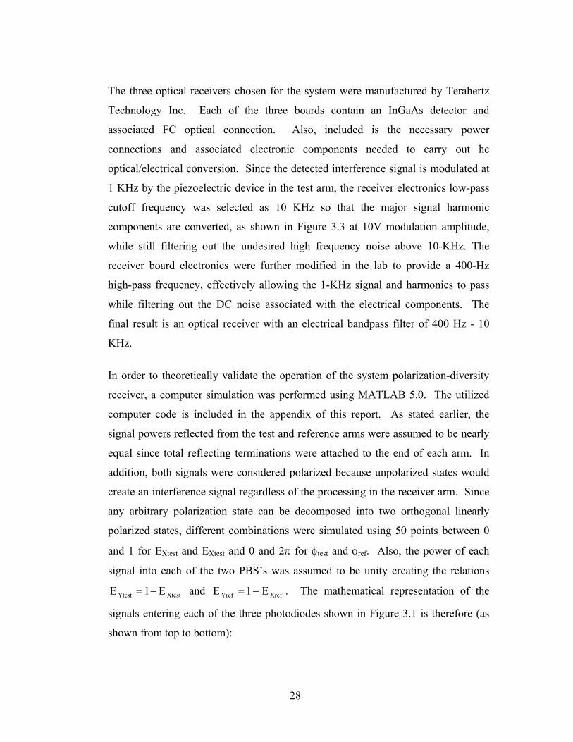
signals entering each of the three photodiodes shown in Figure 3.1 is therefore (as

shown from top to bottom):

29

XrefXtest EE

( )( )reftest jYrefXref

jYtestXtest eEEeEE

21 φφ ++

( )( )reftest jYrefXref

jYtestXtest eEEeEE

21 φφ −+

In order to simulate the total received signal at the photodiode outputs, the

magnitude of each signal was extracted, since all phase information is lost in the

optical/electrical conversion, and summed to get the total received energy. The final

result indicates that the two-tier receiver arrangement provides for interference

signal detection regardless of the reflected test and reference arm signal polarization

orientation. The implications on simulated received signal energy is a maximum

variation of 6.6821 dB, with the highest received signal energy being 3.8278 dB and

the lowest -2.8543 dB. The most important result is an indication that the received

signal variation is well within a reasonable range of detection.

The electrical signal acquisition from the receiver arm is provided by a data

acquisition card interfaced with a personal computer. The signal output of each

photodiode receiver board is sent to a National Instruments SCB-68 terminal block

interface. This device also provides an analog output channel to drive the

piezoelectric modulating device in the test arm. Through the terminal block, the

three corresponding interference signals are received by a National Instruments PC

data-acquisition card, model AT-MIO-16XE-10, where they undergo an analog-to-

digital (A/D) conversion for processing by the PC. Within the PC, further signal

processing is provided using LabVIEW Version 6 graphical programming software,

also from National Instruments. Additionally, this software supplies the tools

needed to construct a graphical interface to display the experimental results.

Specific aspects of the LabVIEW programming are discussed in the next section.

30

Chapter 4: System Operation

4.1 Physical Assembly & Component Power

This and the following sections will provide a comprehensive guide with respect to

the operation of the previously described components as an entire system. A

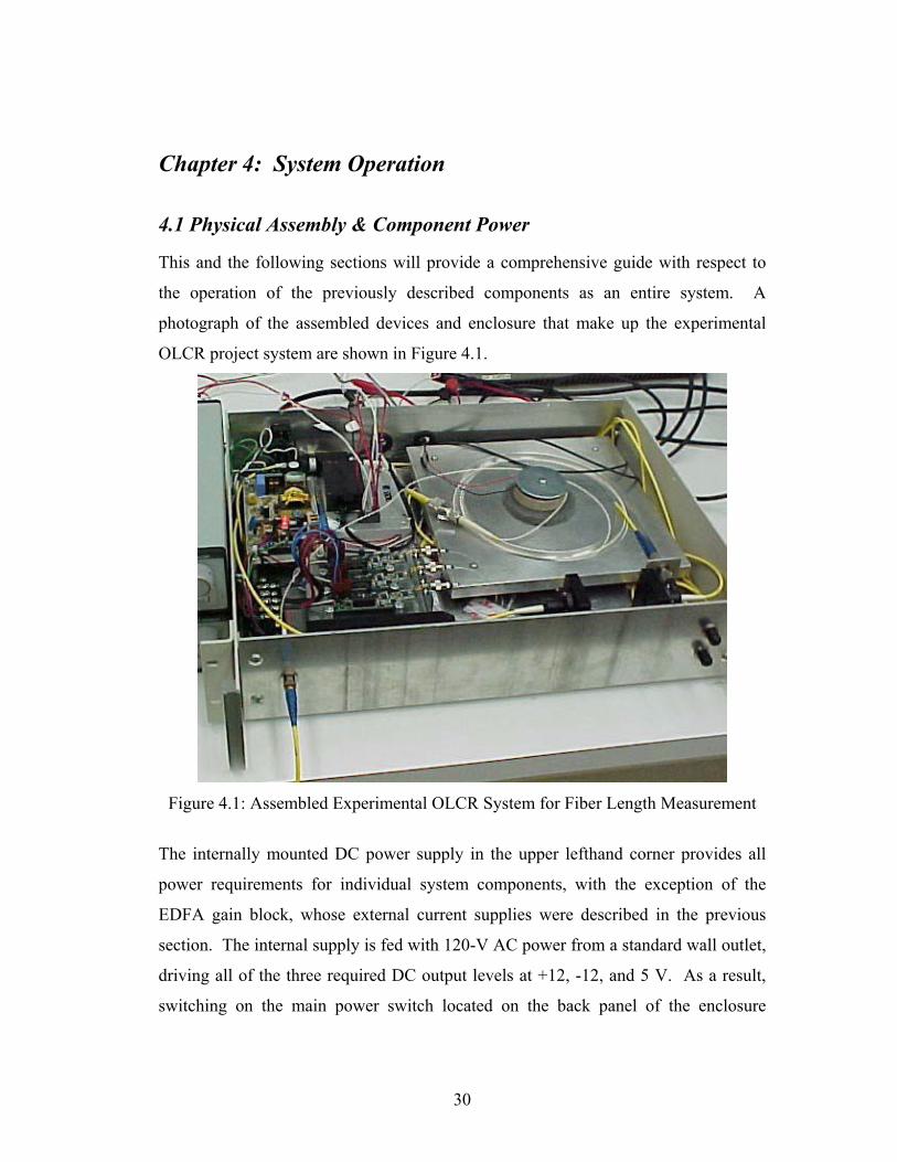
photograph of the assembled devices and enclosure that make up the experimental

OLCR project system are shown in Figure 4.1.

Figure 4.1: Assembled Experimental OLCR System for Fiber Length Measurement

The internally mounted DC power supply in the upper lefthand corner provides all

power requirements for individual system components, with the exception of the

EDFA gain block, whose external current supplies were described in the previous

section. The internal supply is fed with 120-V AC power from a standard wall outlet,

driving all of the three required DC output levels at +12, -12, and 5 V. As a result,

switching on the main power switch located on the back panel of the enclosure

31

activates the DC power supply, which subsequently powers up the tunable optical

filter, fiber scanning delay line, and each photodiode receiver board, initiating all of

them for use. The temperature control and laser driver modules for the EDFA can be

powered up before or after the main system power is switched on, but must be

activated before full system operation can proceed. Additionally, one end of the

length of test arm fiber to be tested is connected to the single front panel connector on

the left side of the front panel. Similarly, an equal length of fiber must be inserted in

the reference arm by connecting each end of the cable to the pair of connectors on the

right side of the panel. All connections between the system enclosure, PC, and

termination block should remain intact regardless of system state or configuration.

These steps complete the physical assembly of the entire system, preparing it for

signal measurement, processing, and data acquisition functions.

4.2 Software & Programming

As indicated earlier, LabVIEW Version 6 graphical programming software is utilized

to construct all aspects of signal processing and graphical display performed in the

operation of the system. The software code will be presented and discussed

graphically in the order in which it is executed in the program file, just as it is

constructed within LabVIEW.

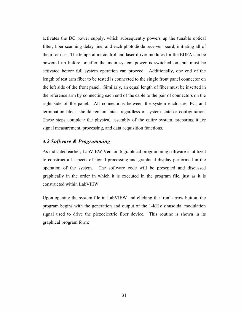
Upon opening the system file in LabVIEW and clicking the ‘run’ arrow button, the

program begins with the generation and output of the 1-KHz sinusoidal modulation

signal used to drive the piezoelectric fiber device. This routine is shown in its

graphical program form:

32

Figure 4.2: Graphical LabVIEW Routine for 1-KHz Sinusoidal Modulation Signal

As evident from the figure, the discrete sinusoidal signal values are generated with a

built-in LabVIEW function at a rate of 100 KHz in order to provide a smooth curve

for the 1-KHz output analog waveform channel. In order to scale the standard output

voltage from the PC card, each value was multiplied by a factor of 5 in order to yield

a 5-V amplitude, as defined earlier in the discussion on modulation signal selection.

This modulation routine is the only part of the overall system program required to run

constantly during all other sequenced operations, unless terminated specifically by the

user.

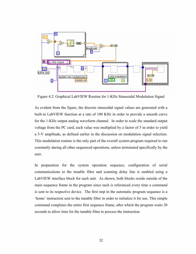
In preparation for the system operation sequence, configuration of serial

communications to the tunable filter and scanning delay line is enabled using a

LabVIEW interface block for each unit. As shown, both blocks reside outside of the

main sequence frame in the program since each is referenced every time a command

is sent to its respective device. The first step in the automatic program sequence is a

‘home’ instruction sent to the tunable filter in order to initialize it for use. This simple

command completes the entire first sequence frame, after which the program waits 20

seconds to allow time for the tunable filter to process the instruction.

33

Figure 4.3: Program Serial Communication Blocks and Tunable Filter Initialization

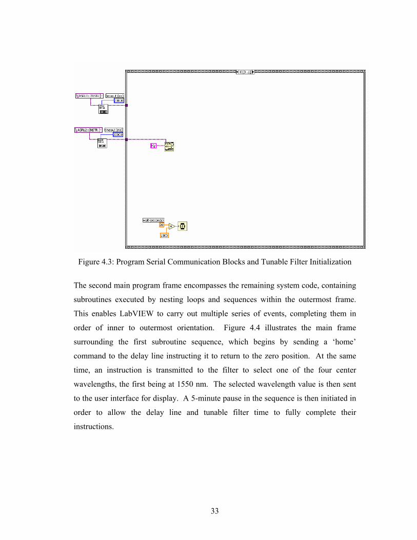
The second main program frame encompasses the remaining system code, containing

subroutines executed by nesting loops and sequences within the outermost frame.

This enables LabVIEW to carry out multiple series of events, completing them in

order of inner to outermost orientation. Figure 4.4 illustrates the main frame

surrounding the first subroutine sequence, which begins by sending a ‘home’

command to the delay line instructing it to return to the zero position. At the same

time, an instruction is transmitted to the filter to select one of the four center

wavelengths, the first being at 1550 nm. The selected wavelength value is then sent

to the user interface for display. A 5-minute pause in the sequence is then initiated in

order to allow the delay line and tunable filter time to fully complete their

instructions.

34

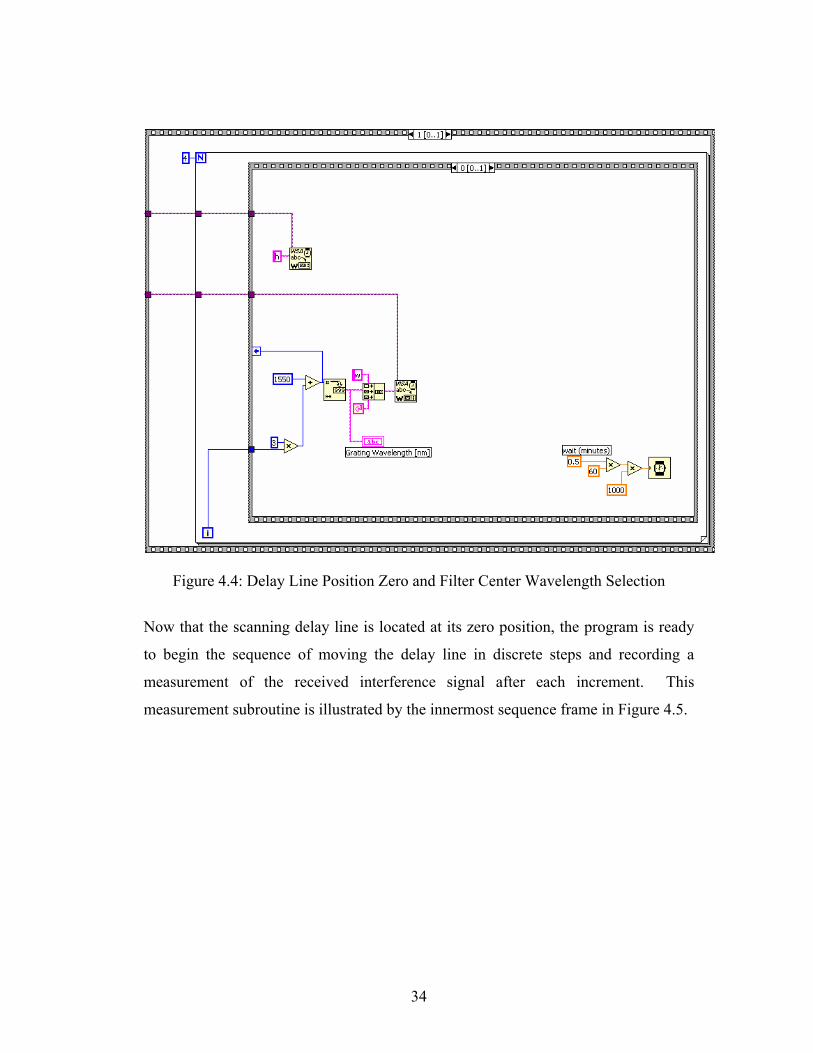
Figure 4.4: Delay Line Position Zero and Filter Center Wavelength Selection

Now that the scanning delay line is located at its zero position, the program is ready

to begin the sequence of moving the delay line in discrete steps and recording a

measurement of the received interference signal after each increment. This

measurement subroutine is illustrated by the innermost sequence frame in Figure 4.5.

35

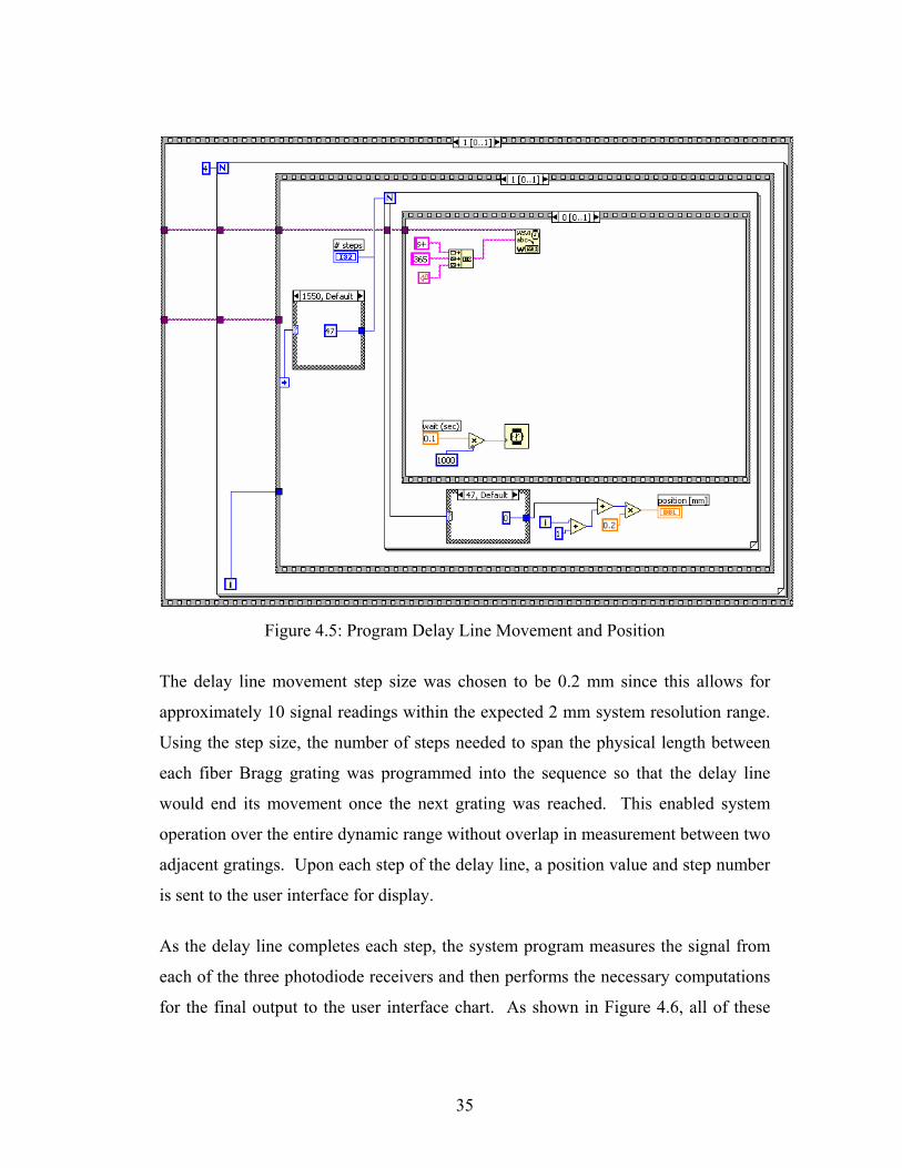
Figure 4.5: Program Delay Line Movement and Position

The delay line movement step size was chosen to be 0.2 mm since this allows for

approximately 10 signal readings within the expected 2 mm system resolution range.

Using the step size, the number of steps needed to span the physical length between

each fiber Bragg grating was programmed into the sequence so that the delay line

would end its movement once the next grating was reached. This enabled system

operation over the entire dynamic range without overlap in measurement between two

adjacent gratings. Upon each step of the delay line, a position value and step number

is sent to the user interface for display.

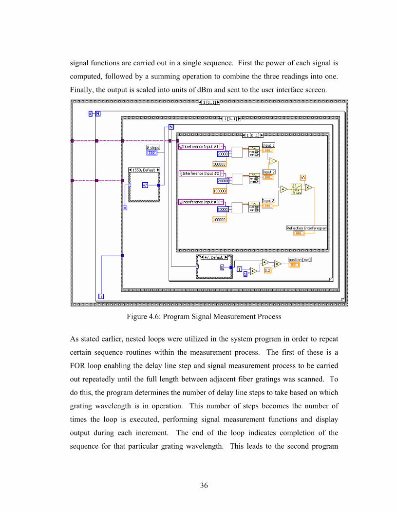
As the delay line completes each step, the system program measures the signal from

each of the three photodiode receivers and then performs the necessary computations

for the final output to the user interface chart. As shown in Figure 4.6, all of these

36

signal functions are carried out in a single sequence. First the power of each signal is

computed, followed by a summing operation to combine the three readings into one.

Finally, the output is scaled into units of dBm and sent to the user interface screen.

Figure 4.6: Program Signal Measurement Process

As stated earlier, nested loops were utilized in the system program in order to repeat

certain sequence routines within the measurement process. The first of these is a

FOR loop enabling the delay line step and signal measurement process to be carried

out repeatedly until the full length between adjacent fiber gratings was scanned. To

do this, the program determines the number of delay line steps to take based on which

grating wavelength is in operation. This number of steps becomes the number of

times the loop is executed, performing signal measurement functions and display

output during each increment. The end of the loop indicates completion of the

sequence for that particular grating wavelength. This leads to the second program

37

FOR loop, which is utilized to repeat the entire stepping and measurement process for

each of the four grating wavelengths. The start of this loop signals the delay line to

return to zero position in preparation for the step and measurement sequence loop

described earlier. In addition, the grating wavelength is selected with the tunable

filter, starting with the first centered at 1550 nm. Upon completion of the entire

measurement process, the loop selects the next wavelength at 1553, while at the same

time instructing the delay line to return to zero position once again. This method is

carried out a total of four times, once for each of the fiber Bragg grating wavelengths.

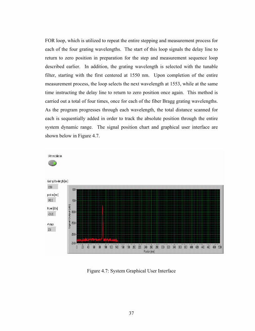
As the program progresses through each wavelength, the total distance scanned for

each is sequentially added in order to track the absolute position through the entire

system dynamic range. The signal position chart and graphical user interface are

shown below in Figure 4.7.

Figure 4.7: System Graphical User Interface

38

As the system position approaches the point of reference and test arm length

equivalency, a sharp peak in the measurement output will be observed on the chart.

Once the program has completely scanned the system dynamic range, this peak can

be located in the output data and the position recorded. Therefore each time the

system program is run, the peak position value can be recorded and tracked for

changes in the fiber length. This enables the system for use in tracking crustal

deformation changes by way of measurement changes in a buried fiber section, as

described earlier in this report. In addition, the system may find uses in any instance

where high resolution is desired for long fiber length measurement.

39

Chapter 5: Summary of Results and Conclusions

Based on the success of conventional OLCR measurement, its well-established basic

system arrangement was ideal for use as the foundation for a unique approach to long

fiber length measurement. As a result, the project system development could focus

on the novel techniques enabling it for use in an application not normally considered

practical for conventional OLCR. The following overall project results will therefore

emphasize the performance of these new methods, since standard OLCR system

operation has been well documented. Consequently, the measures of performance

presented for the experimental system are similar to those used in evaluating other

optical length measurement devices including other OLCR arrangements.

One common measure of system performance is the dynamic measurement range,

used to determine the maximum change in length that can be detected during

operation. In this project it similarly describes the maximum acceptable length

difference between the reference and test arm fiber sections. It is important in a

crustal drift measurement application to have a dynamic range large enough to

accommodate buried fiber length changes of up to 20 cm/year. Therefore the goal of

this project was to develop a range of several meters through a series of fiber Bragg

gratings in the system reference arm. As described earlier, the fiber distance between

each grating directly added to the basic dynamic range of the scanning delay line.

Therefore, the four gratings added the following measured distances to the overall

system range: 9.39 cm (1550-1553 nm), 7.44 cm (1553-1556 nm), and 7.39 cm

(1556-1559 nm). Additionally, the double-pass delay line arrangement extended its

scanning range to 17.0 cm, yielding an overall system dynamic measurement range of

41.22 cm. Even though this result falls short of the project goal of several meters of

range, the fiber grating method of range extension clearly demonstrates the

opportunity to meet this goal by simply adding the appropriate number of additional

gratings, at other wavelengths within the spectral width of the EDFA source. In fact,

if the entire 33-nm spectral width was exploited, a total of 22 fiber Bragg gratings

40

with a bandwidth of 1.5 nm could be utilized. In addition, each grating could be

spaced up to the 17-cm scanning range of the delay line yielding a total dynamic

range of 3.74 meters, thus exceeding the goal of the project. Because of time

constraints on the project, the work needed to attain this dynamic range could not be

realized, however, the enabling method was clearly demonstrated.

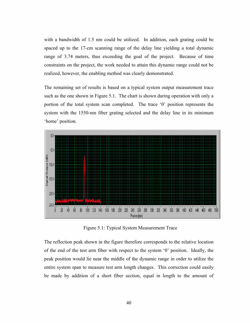
The remaining set of results is based on a typical system output measurement trace

such as the one shown in Figure 5.1. The chart is shown during operation with only a

portion of the total system scan completed. The trace ‘0’ position represents the

system with the 1550-nm fiber grating selected and the delay line in its minimum

‘home’ position.

Figure 5.1: Typical System Measurement Trace

The reflection peak shown in the figure therefore corresponds to the relative location

of the end of the test arm fiber with respect to the system ‘0’ position. Ideally, the

peak position would lie near the middle of the dynamic range in order to utilize the

entire system span to measure test arm length changes. This correction could easily

be made by addition of a short fiber section, equal in length to the amount of

41

adjustment needed, to either the reference or test arm, depending on which direction

the peak position is to be moved.

The system noise floor, as indicated on the graphic display, resides at approximately

–23 dBm. In comparison to conventional OLCR systems, this level of noise is

significantly worse than normally observed. However, typical OLCR requires a high

level of sensitivity (low noise floor) in order to detect weak reflections in the test arm.

For the designed project application, as discussed earlier, the test arm fiber is

terminated with a highly reflective end, thus resulting in a strong signal to be

detected. As a result, the more important performance metric in this case is the level

of measured interference signal with respect to the noise floor. As shown in the

typical trace peak, the measured value is approximately –7 dBm, which represents a

level 16 dB above the system sensitivity limit. Since the reflected test and reference

arm signals are relatively constant throughout operation, the detected measurement

peak level remains well above the sensitivity limit regardless of position. In addition,

the maximum penalty for the polarization diversity receiver was shown analytically to

be no greater than 7 dB, resulting in a minimum peak level of at least –14 dBm and

therefore a system sensitivity that is adequate for the full range of system operation.

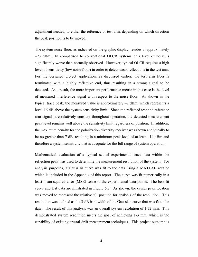
Mathematical evaluation of a typical set of experimental trace data within the

reflection peak was used to determine the measurement resolution of the system. For

analysis purposes, a Gaussian curve was fit to the data using a MATLAB routine

which is included in the Appendix of this report. The curve was fit numerically in a

least mean-squared-error (MSE) sense to the experimental data points. The best-fit

curve and test data are illustrated in Figure 5.2. As shown, the center peak location

was moved to represent the relative ‘0’ position for analysis of the resolution. This

resolution was defined as the 3-dB bandwidth of the Gaussian curve that was fit to the

data. The result of this analysis was an overall system resolution of 1.72 mm. This

demonstrated system resolution meets the goal of achieving 1-3 mm, which is the

capability of existing crustal drift measurement techniques. This project outcome is

42

another very important step towards the viability of system use in a crustal

measurement application.

-4 -3 -2 -1 0 1 2 3 4-24

-22

-20

-18

-16

-14

-12

-10

-8

-6

distance [mm]

pow

er [d

B]

Figure 5.2: Reflection Peak Data and Gaussian Curve Fit

The final assessment of system performance involves the evaluation of the

polarization-diversity receiver. In actuality, this task proved to be difficult to quantify

in the process of experimental testing. In addition, time constraints upon completion

of the system assembly minimized the amount of testing that could be dedicated to

the receiver scheme. However, the main objective in incorporating the passive-type

receiver scheme was to allow the system continuous interference signal detection

without needed adjustments or corrections based on the polarization states of the

incoming signals. By all experimental accounts, the receiver scheme exceeded the

performance predicted by the numerical simulations described earlier in this report.

The calculated penalty to system performance from the polarization-diversity scheme

43

was a maximum of approximately 7 dB, while the observed output interference signal

varied no more than a few dB for the entire time spent recording data. More

importantly, the detection of a signal measurement peak was observed during every

system scan, regardless of the position within the total dynamic range. Therefore, the

receiver successfully detected an interference signal each time one was expected,

throughout the entire experimental evaluation time. Additional testing with longer

fiber sections will prove to be a more thorough long-term evaluation of the receiver

scheme. In addition, polarization controllers in each of the test and reference arms

would provide a realization and validation of the numerical evaluation performed for

the project. These and other possible system enhancements will be further discussed

in the next section.

A summary of the project measurement system results illustrates the viability of its

use in the application of crustal deformation measurement. This includes the

demonstration of a method for realizing a system dynamic range of nearly 4 meters

through the utilization of fiber Bragg gratings in the system reference arm. This

dynamic range will enable the tracking of movement up to 20 cm/yr over a period of

many years. Also, the demonstrated system resolution of 1.72 mm is in the range of

currently used methods of crustal drift. However, the appeal of a buried fiber-based

method is the exploitation of a stable measurement environment such as the Earth’s

crust itself. With these system performance metrics demonstrated, the project can be

considered an important advancement in the high-resolution measurement of long

optical fibers.

44

Chapter 6: Future Work

With the project demonstration of a long fiber length change measurement system,

one can look beyond the intended use in quantifying crustal deformation and begin to

consider other applications. The short-term focus of future work to be explored could

be additional system operational enhancements to improve aspects such as

measurement functions or accuracy. However, longer-term system component and

arrangement modifications look to be more promising, since this work may lead to a

number of new applications based on the proven existing system. Therefore, the

remainder of this section will focus on advanced work enabling the project system for

potential use in other aspects of optical length measurement.

The first area of future development is for system use in long fiber fault detection,

currently measured using OTDR systems which use short optical pulses in the time

domain. This allows OTDR a dynamic range of several tens of kilometers or more,

depending on the device power. The disadvantage of this method is a measurement

resolution of several meters, at best, when measuring long fiber sections. Therefore,

the use of a frequency-domain device, such as the developed project system, proves

desirable based on the millimeter-range resolution capable of more accurately

locating a fiber fault. The constraint in this case is a dynamic range of only a few

meters, preventing the ability to detect a fault over a range of several kilometers as in

OTDR. As a result, the combined use of both techniques may provide a useful

solution to millimeter-accurate detection of long fiber faults, using OTDR to narrow

the location down to several meters and the project OLCR system to further pinpoint

the fault. The key change within the project system would be the need to detect weak

fiber reflections such as those common to faults. As discussed earlier, the current

system receiver operation was developed based on similar signal powers returning

from the test and reference arms. In order to provide for fiber fault detection, the

polarization-diversity scheme would need to be expanded to allow for a weakly

reflected signal from the test arm. This scheme could be realized by adding

45

additional polarization components in the current receiver arm configuration. The

passive operation of the receiver could remain or one may choose to develop an

active scheme to handle the weak fault detection. Either way, the concept of

millimeter-accurate fiber fault detection proves to be a promising possibility for

future work on the project OLCR system.

Another area of future development is to expand the use of conventional OLCR

beyond the current range limitations of approximately 10 cm. This method typically

uses a wide spectral width source enabling a measurement resolution down to several

micrometers. However, in the rapidly expanding area of optical networking,

component arrangements can easily extend beyond the 10 cm range of conventional

dynamic operation. In order to characterize the reflections from such an arrangement,

the project OLCR system could provide the required dynamic range extension. The

project technique for range expansion does result in a loss of resolution, however this

may be acceptable in cases where micrometer accuracy is not required for reflection

characterization. Existing methods for polarization control could be utilized or the

system polarization diversity receiver could be modified to allow for weakly reflected

signals in the test arm, as in the previously-described fault detection application. The

method for doing so could be the same in both cases.

As evident from the potential new applications, the utilization of the measurement

system developed in this project could greatly expanded through the development of a

polarization-diversity receiver capable of operating with weakly reflected signals

from the test arm. This would enable accurate location detection of fiber and optical

component faults in a large number of applications. Also, as with any new

technology, many currently unknown applications may arise to make use of the new

methods developed for this project measurement system. Either way, the system

looks to be an important advancement in the demonstrated techniques for OLCR

dynamic range extension and polarization-diversity detection.

46

References

[1] D. Derickson, Fiber Optic Test and Measurement, Prentice Hall PTR (1998).

[2] U. Wiedman and P. Gallion, “A Generalized Approach to Optical Low-Coherence

Reflectometry Including Spectral Filtering Effects,” Journal of Lightwave

Technology, Vol. 16, No. 7, July 1998.

[3] S. Mechels, K. Takada, and K. Okamoto, “Optical Low-Coherence Reflectometer

for Measuring WDM Component,” IEEE Photonics Technology Letters, Vol. 11,

No. 7, July 1999.

[4] M. Volanthen, H. Geiger, and J.P. Dakin, “Distributed Grating Sensors Using

Optical Low-Coherence Reflectometry,” Journal of Lightwave Technology, Vol.

15, No. 11, November 1997.

[5] H.H. Gilgen, R.P. Novak, R.P. Salathe, W. Hodel, and P. Beaud, “Submillimeter

Optical Reflectometry,” Journal of Lightwave Technology, Vol. 7, No. 8, August

1989.

[6] D.M. Baney and W.V. Sorin, “Extended-Range Optical Low-Coherence

Reflectometry Using a Recirculating Delay Technique,” IEEE Photonics

Technology Letters, Vol. 5, No. 9, September 1993.

[7] K. Takada and M. Horiguchi, “Jaggedness-Free Millimeter-Resolution Low-

Coherence Reflectometry,” Journal of Lightwave Technology, Vol. 12, No. 4,

April 1994.

47

[8] K. Takada, M. Yamada, and S. Mitachi, “Optical Low Coherence Reflectometer

with a 47-dB Dynamic Range Achieved by Using a Flouride-Based Erbium-

Doped Fiber Amplifier,” Journal of Lightwave Technology, Vol. 16, No. 4, April

1998.

[9] T. Saida and K. Hotate, “Distributed Fiber-Optic Stress Sensor by Synthesis of

the Optical Coherence Function,” IEEE Photonics Technology Letters, Vol. 9,

No. 4, April 1997.

[10] W.V. Sorin and D.M. Baney, “Measurement of Rayleigh Backscattering at 1.55

µm with 32 µm Spatial Resolution,” IEEE Photonics Technology Letters, Vol. 4,

No. 4, April 1992.

[11] K.O. Hill and G. Meltz, “Fiber Bragg Grating Technology Fundamentals and

Overview,” Journal of Lightwave Technology, Vol. 15, No. 8, August 1997.

[12] K. Takada, M. Yamada, Y. Hibino, and S. Mitachi, “Range Extension in Optical

Low Coherence Reflectometry Achieved by Using a Pair of Retroreflectors,”

Electronics Letters, Vol. 31, 1995.

[13] M. Ming-Kang Lui, Principles and Applications of Optical Communications,

Chicago: Irwin, 1996.

[14] G. Keiser, Optical Fiber Communications, New York: McGraw-Hill, 2000.

[15] T. Erdogan, “Fiber Grating Spectra,” Journal of Lightwave Technology, vol. 15,

pp. No. 8, 1997.

48

[16] C. R. Giles, “Lightwave Applications of Fiber Bragg Gratings,” Journal of

Lightwave Technology, vol. 15, No. 8, 1997.

[17] B. L. Danielson and C. D. Whittenberg, “Guided-Wave Reflectometry with

Micrometer Resolution,” Applied Optics, vol. 26, No. 14, 1987.

[18] W.V. Sorin and D.M. Baney, “A Simple Intensity Noise Reduction Technique

for Optical Low-Coherence Reflectometry,” IEEE Photonics Technology Letters,

Vol. 5, No. 9, September 1993.

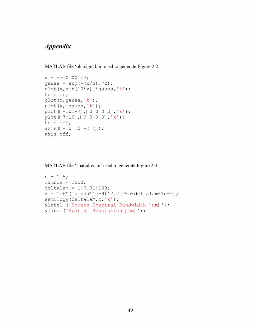
49

Appendix

MATLAB file ‘olcrsignal.m’ used to generate Figure 2.2: x = -7:0.001:7; gauss = exp(-(x/3).^2); plot(x,sin(10*x).*gauss,'k'); hold on; plot(x,gauss,'k'); plot(x,-gauss,'k'); plot([-10:-7],[0 0 0 0],'k'); plot([7:10],[0 0 0 0],'k'); hold off; axis([-10 10 -2 2]); axis off;

MATLAB file ‘spatialres.m’ used to generate Figure 2.3: n = 1.5; lambda = 1550; deltalam = 1:0.01:100; z = 1e6*(lambda*1e-9)^2./(2*n*deltalam*1e-9); semilogy(deltalam,z,'k'); xlabel ('Source Spectral Bandwidth [nm]'); ylabel('Spatial Resolution [um]');

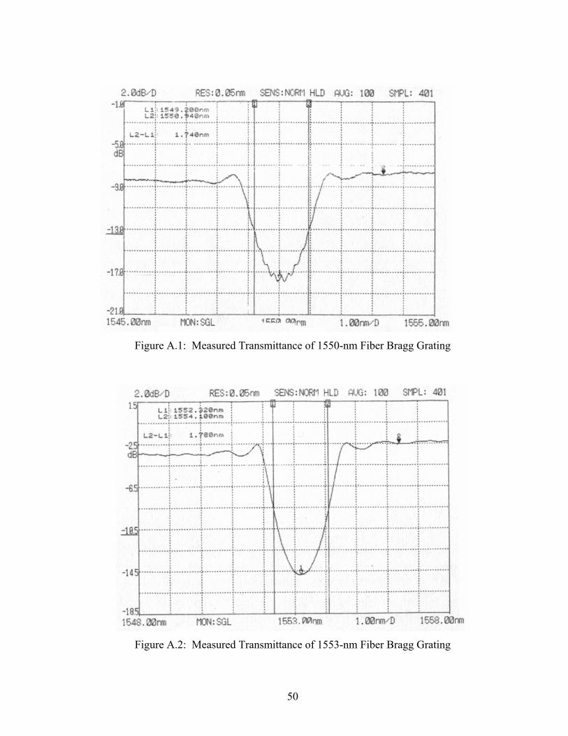
50

Figure A.1: Measured Transmittance of 1550-nm Fiber Bragg Grating

Figure A.2: Measured Transmittance of 1553-nm Fiber Bragg Grating

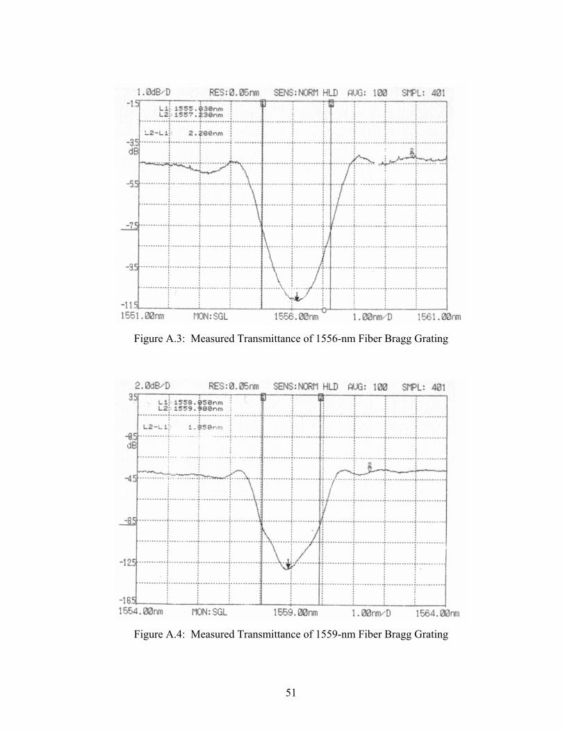
51

Figure A.3: Measured Transmittance of 1556-nm Fiber Bragg Grating

Figure A.4: Measured Transmittance of 1559-nm Fiber Bragg Grating

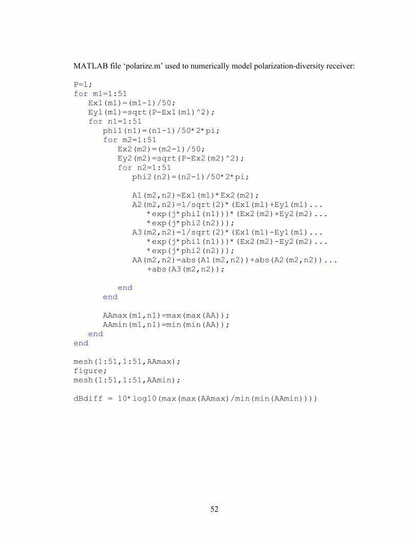
52

MATLAB file ‘polarize.m’ used to numerically model polarization-diversity receiver: P=1; for m1=1:51 Ex1(m1)=(m1-1)/50; Ey1(m1)=sqrt(P-Ex1(m1)^2); for n1=1:51 phi1(n1)=(n1-1)/50*2*pi; for m2=1:51 Ex2(m2)=(m2-1)/50; Ey2(m2)=sqrt(P-Ex2(m2)^2); for n2=1:51 phi2(n2)=(n2-1)/50*2*pi; A1(m2,n2)=Ex1(m1)*Ex2(m2); A2(m2,n2)=1/sqrt(2)*(Ex1(m1)+Ey1(m1)... *exp(j*phi1(n1)))*(Ex2(m2)+Ey2(m2)... *exp(j*phi2(n2))); A3(m2,n2)=1/sqrt(2)*(Ex1(m1)-Ey1(m1)... *exp(j*phi1(n1)))*(Ex2(m2)-Ey2(m2)... *exp(j*phi2(n2))); AA(m2,n2)=abs(A1(m2,n2))+abs(A2(m2,n2))... +abs(A3(m2,n2)); end end AAmax(m1,n1)=max(max(AA)); AAmin(m1,n1)=min(min(AA)); end end mesh(1:51,1:51,AAmax); figure; mesh(1:51,1:51,AAmin); dBdiff = 10*log10(max(max(AAmax)/min(min(AAmin))))

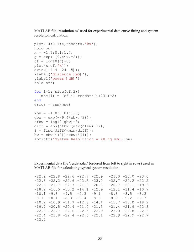
53

MATLAB file ‘resolution.m’ used for experimental data curve fitting and system resolution calculation: plot(-4:0.1:4,resdata,'kx'); hold on; x = -1.7:0.1:1.7; g = exp(-(9.4*x.^2)); cf = log10(g)-8; plot(x,cf,'k'); axis([-4 4 -24 -5]); xlabel('distance [mm]'); ylabel('power [dB]'); hold off; for i=1:(size(cf,2)) mse(i) = (cf(i)-resdata(i+23))^2; end error = sum(mse) xbw = -1.0:0.01:1.0; gbw = exp(-(9.4*xbw.^2)); cfbw = log10(gbw)-8; diff = abs(cfbw-(max(cfbw)-3)); i = find(diff<=min(diff)); bw = xbw(i(2))-xbw(i(1)); sprintf('System Resolution = %0.5g mm', bw)

Experimental data file ‘resdata.dat’ (ordered from left to right in rows) used in MATLAB file for calculating typical system resolution: -22.9 -22.8 -22.6 -22.7 -22.9 -23.0 -23.0 -23.0 -22.6 -22.2 -22.6 -22.6 -23.0 -22.7 -22.2 -22.2 -22.6 -21.7 -22.3 -21.0 -20.8 -20.7 -20.1 -19.3 -18.2 -16.5 -15.2 -14.1 -12.9 -12.1 -11.4 -10.7 -10.1 -9.8 -9.5 -9.3 -9.1 -8.8 -8.5 -8.3 -8.1 -8.1 -8.3 -8.4 -8.6 -8.9 -9.2 -9.7 -10.2 -10.9 -11.7 -12.8 -14.4 -15.7 -17.0 -18.2 -19.7 -20.5 -20.4 -21.0 -21.3 -21.4 -21.9 -22.3 -22.3 -22.7 -22.6 -22.5 -22.9 -23.0 -22.8 -22.6 -22.4 -21.8 -22.4 -22.6 -22.1 -22.9 -22.9 -22.7 -22.7

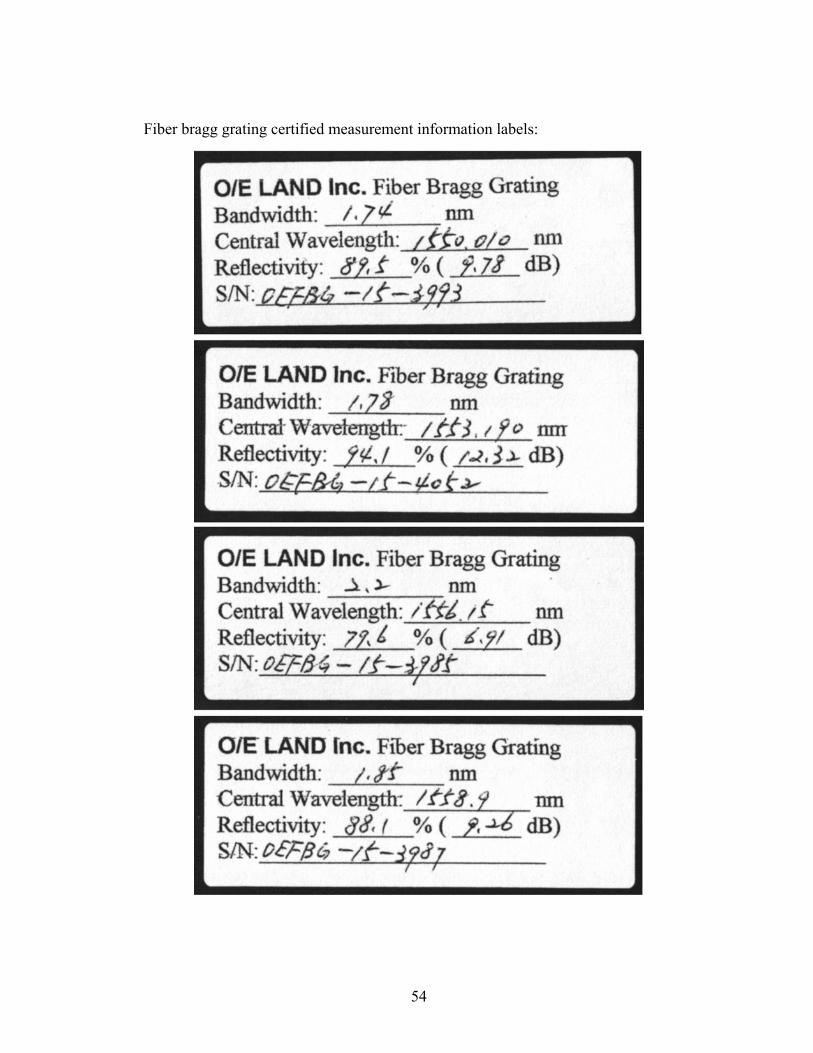
54

Fiber bragg grating certified measurement information labels:

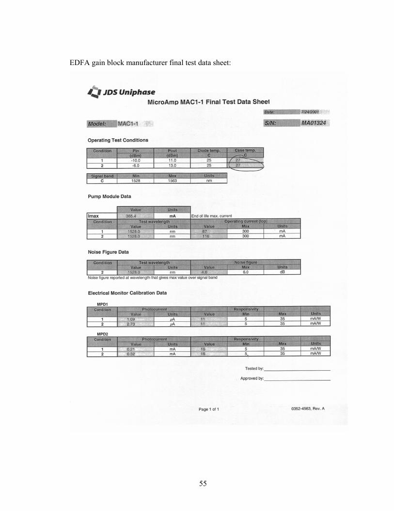
55

EDFA gain block manufacturer final test data sheet:

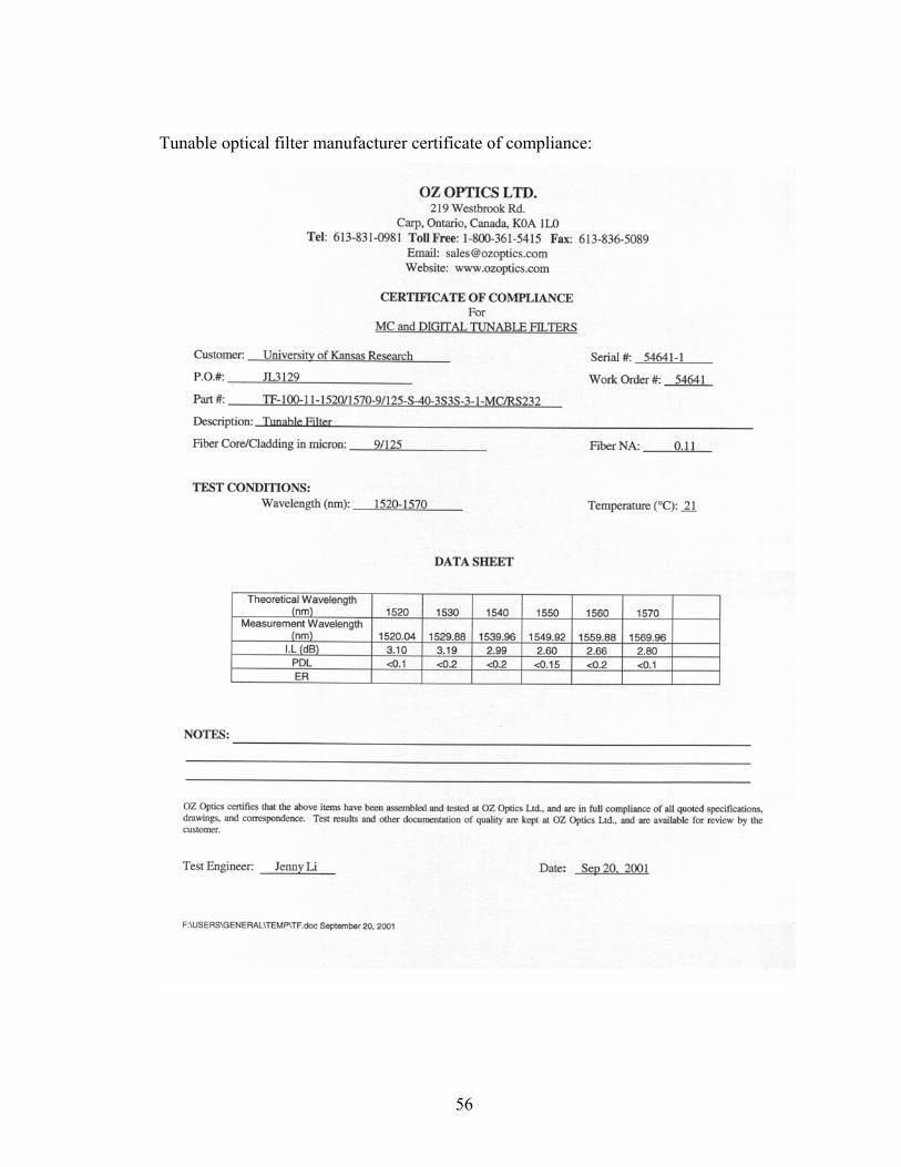
56

Tunable optical filter manufacturer certificate of compliance: