Embed Size (px)
Citation preview
Chapter 2
Introduction to Statistics
Contents2.1 TRRGET - An overview of statistical inference . . . . . . . . . . . . . . . . . . . 352.2 Parameters, Statistics, Standard Deviations, and Standard Errors . . . . . . . . . 38
2.2.1 A review . . . . . . . . . . . . . . . . . . . . . . . . . . . . . . . . . . . . . 392.2.2 Theoretical example of a sampling distribution . . . . . . . . . . . . . . . . . 45
2.3 Confidence Intervals . . . . . . . . . . . . . . . . . . . . . . . . . . . . . . . . . . 462.3.1 A review . . . . . . . . . . . . . . . . . . . . . . . . . . . . . . . . . . . . . 472.3.2 Some practical advice . . . . . . . . . . . . . . . . . . . . . . . . . . . . . . 532.3.3 Technical details . . . . . . . . . . . . . . . . . . . . . . . . . . . . . . . . . 54
2.4 Hypothesis testing . . . . . . . . . . . . . . . . . . . . . . . . . . . . . . . . . . . 542.4.1 A review . . . . . . . . . . . . . . . . . . . . . . . . . . . . . . . . . . . . . 552.4.2 Comparing the population parameter against a known standard . . . . . . . . 552.4.3 Comparing the population parameter between two groups . . . . . . . . . . . 622.4.4 Type I, Type II and Type III errors . . . . . . . . . . . . . . . . . . . . . . . 652.4.5 Some practical advice . . . . . . . . . . . . . . . . . . . . . . . . . . . . . . 682.4.6 The case against hypothesis testing . . . . . . . . . . . . . . . . . . . . . . . 692.4.7 Problems with p-values - what does the literature say? . . . . . . . . . . . . . 71
2.5 Meta-data . . . . . . . . . . . . . . . . . . . . . . . . . . . . . . . . . . . . . . . . 732.5.1 Scales of measurement . . . . . . . . . . . . . . . . . . . . . . . . . . . . . 732.5.2 Types of Data . . . . . . . . . . . . . . . . . . . . . . . . . . . . . . . . . . 752.5.3 Roles of data . . . . . . . . . . . . . . . . . . . . . . . . . . . . . . . . . . 76
2.6 Bias, Precision, Accuracy . . . . . . . . . . . . . . . . . . . . . . . . . . . . . . . 762.7 Types of missing data . . . . . . . . . . . . . . . . . . . . . . . . . . . . . . . . . . 782.8 Transformations . . . . . . . . . . . . . . . . . . . . . . . . . . . . . . . . . . . . 80
2.8.1 Introduction . . . . . . . . . . . . . . . . . . . . . . . . . . . . . . . . . . . 802.8.2 Conditions under which a log-normal distribution appears . . . . . . . . . . . 812.8.3 ln() vs. log() . . . . . . . . . . . . . . . . . . . . . . . . . . . . . . . . . . 822.8.4 Mean vs. Geometric Mean . . . . . . . . . . . . . . . . . . . . . . . . . . . 822.8.5 Back-transforming estimates, standard errors, and ci . . . . . . . . . . . . . . 832.8.6 Back-transforms of differences on the log-scale . . . . . . . . . . . . . . . . 842.8.7 Some additional readings on the log-transform . . . . . . . . . . . . . . . . . 85
2.9 Standard deviations and standard errors revisited . . . . . . . . . . . . . . . . . . 962.10 Other tidbits . . . . . . . . . . . . . . . . . . . . . . . . . . . . . . . . . . . . . . 102
2.10.1 Interpreting p-values . . . . . . . . . . . . . . . . . . . . . . . . . . . . . . 102
34
CHAPTER 2. INTRODUCTION TO STATISTICS
2.10.2 False positives vs. false negatives . . . . . . . . . . . . . . . . . . . . . . . . 1032.10.3 Specificity/sensitivity/power . . . . . . . . . . . . . . . . . . . . . . . . . . 103
The suggested citation for this chapter of notes is:
Schwarz, C. J. (2019). Introduction to Statistics.In Course Notes for Beginning and Intermediate Statistics.Available at http://www.stat.sfu.ca/~cschwarz/CourseNotes. Retrieved2019-11-04.
Statistics was spawned by the information age, and has been defined as the science of extractinginformation from data. Technological developments have demanded methodology for the efficient ex-traction of reliable statistics from complex databases. As a result, Statistics has become one of the mostpervasive of all disciplines.
Theoretical statisticians are largely concerned with developing methods for solving the problemsinvolved in such a process, for example, finding new methods for analyzing (making sense of) types ofdata that existing methods cannot handle. Applied statisticians collaborate with specialists in other fieldsin applying existing methodologies to real world problems. In fact, most statisticians are involved inboth of these activities to a greater or lesser extent, and researchers in most quantitative fields of enquiryspend a great deal of their time doing applied statistics.
The public and private sector rely on statistical information for such purposes as decision making,regulation, control and planning.
Ordinary citizens are exposed to many ‘statistics’ on a daily basis. For example:
• “In a poll of 1089 Canadians, 47% were in favor of the constitution accord. This result is accurateto within 3 percentage points, 19 time out of 20.”
• “The seasonally adjusted unemployment rate in Canada was 9.3%”.
• “Two out of three dentists recommend Crest.”
What does this all mean?
Our goal is not to make each student a ‘professional statistician’, but rather to give each student asubset of tools with which they can confidently approach many real world problems and make sense ofthe numbers.
2.1 TRRGET - An overview of statistical inference
Section summary:
1. Distinguish between a population and a sample
2. Why it is important to choose a probability sample
3. Distinguish among the roles of randomization, replication, and blocking
c©2019 Carl James Schwarz 35 2019-11-04
CHAPTER 2. INTRODUCTION TO STATISTICS
4. Distinguish between an ‘estimate’ or a ‘statistic’ and the ‘parameter’ of interest.
Most studies can be broadly classified into either surveys or experiments.
In surveys, the researcher is typically interested in describing some population - there is usuallyno attempt to manipulate units within the population. In experiments, units from the population aremanipulated in some fashion and a response to the manipulation is observed.
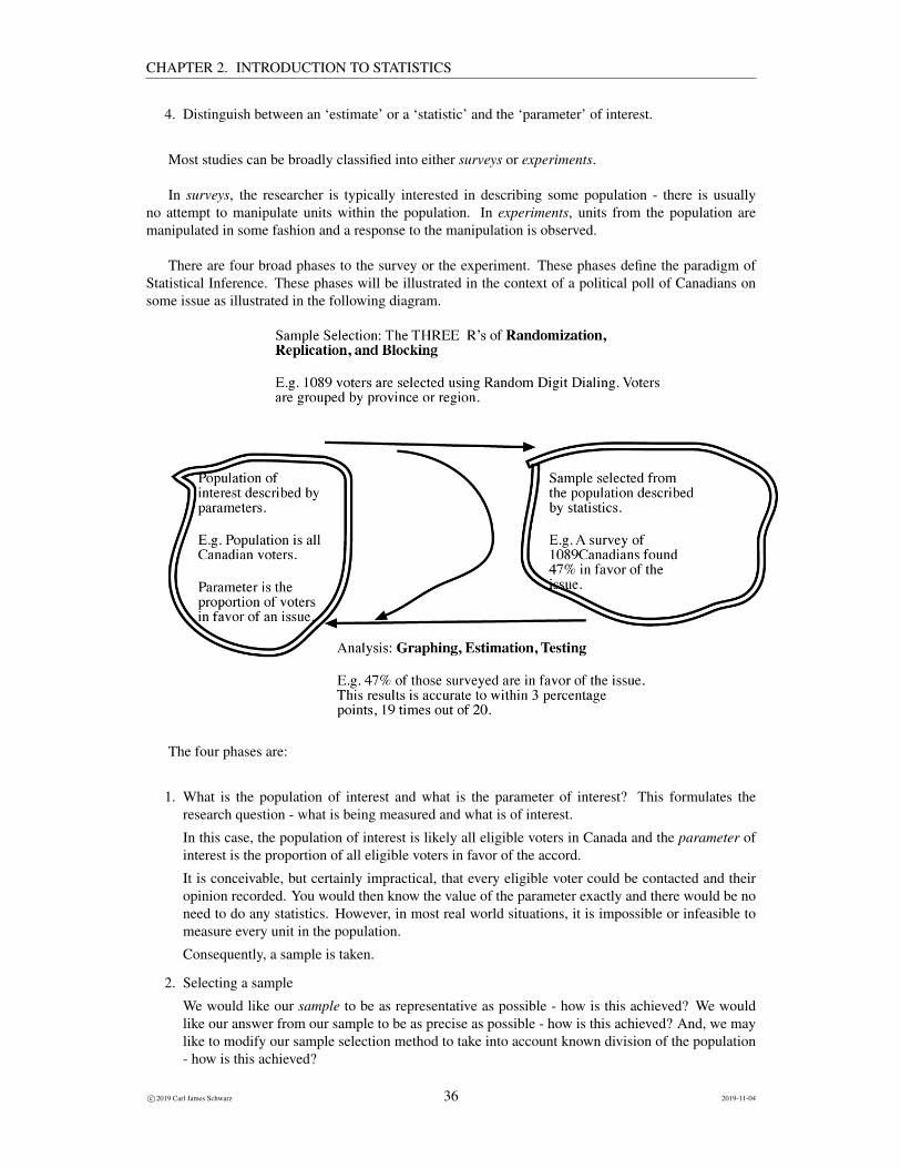
There are four broad phases to the survey or the experiment. These phases define the paradigm ofStatistical Inference. These phases will be illustrated in the context of a political poll of Canadians onsome issue as illustrated in the following diagram.
The four phases are:
1. What is the population of interest and what is the parameter of interest? This formulates theresearch question - what is being measured and what is of interest.
In this case, the population of interest is likely all eligible voters in Canada and the parameter ofinterest is the proportion of all eligible voters in favor of the accord.
It is conceivable, but certainly impractical, that every eligible voter could be contacted and theiropinion recorded. You would then know the value of the parameter exactly and there would be noneed to do any statistics. However, in most real world situations, it is impossible or infeasible tomeasure every unit in the population.
Consequently, a sample is taken.
2. Selecting a sample
We would like our sample to be as representative as possible - how is this achieved? We wouldlike our answer from our sample to be as precise as possible - how is this achieved? And, we maylike to modify our sample selection method to take into account known division of the population- how is this achieved?
c©2019 Carl James Schwarz 36 2019-11-04
CHAPTER 2. INTRODUCTION TO STATISTICS
Three fundamental principles of Statistics are randomization, replication and blocking.
Randomization This is the most important aspect of experimental design and surveys. Random-ization “makes” the sample ‘representative’ of the population by ensuring that, ‘on average’,the sample will contain a proportion of population units that is about equal, for any variableas found in the population.If an experiment is not randomized or a survey is not randomly collected, it rarely (if ever)provides useful information.Many people confuse ‘random’ with ‘haphazard’. The latter only means that the sample wascollected without a plan or thought to ensure that the sample obtained is representative of thepopulation. A truly ‘random’ sample takes surprisingly much effort to collect!E.g. The Gallup poll uses random digit dialing to select at random from all householdsin Canada with a phone. Is this representative of the entire voting population? How doesthe Gallup Poll account for the different patterns of telephone use among genders within ahousehold?A simple random sample is an example of a equal probability sample where every unit inthe population has an equal chance of being selected for the sample. As you will see later inthe notes, the assumption of equal probability of selection not crucial. What is crucial is thatevery unit in the population have a known probability of selection, but this probability couldvary among units. For example, you may decide to sample males with a higher probabilitythan females.
Replication = Sample Size This ensures that the results from the experiment or the survey willbe precise enough to be of use. A large sample size does not imply that the sample is repre-sentative - only randomization ensures representativeness.Do not confuse replication with repeating the survey a second time.In this example, the Gallup poll interviews about 1100 Canadians. It chooses this number ofpeople to get a certain precision in the results.
Blocking (or stratification) In some experiments or surveys, the researcher knows of a variablethat strongly influences the response. In the context of this example, there is strong relation-ship between the region of the country and the response.Consequently, precision can be improved, by first blocking or stratifying the population intomore homogeneous groups. Then a separate randomized survey is done in each and everystratum and the results are combined together at the end.In this example, the Gallup poll often stratifies the survey by region of Canada. Withineach region of Canada, a separate randomized survey is performed and the results are thencombined appropriately at the end.
3. Data Analysis
Once the survey design is finalized and the survey is conducted, you will have a mass of infor-mation - statistics - collected from the population. This must be checked for errors, transcribedusually into machine readable form, and summarized.
The analysis is dependent upon BOTH the data collected (the sample) and the way the data wascollected (the sample selection process). For example, if the data were collected using a stratifiedsampling design, it must be analyzed using the methods for stratified designs - you can’t simplypretend after the fact that the data were collected using a simple random sampling design.
We will emphasize this point continually in this course - you must match the analysis with thedesign!
For example, consider a Gallup Poll where 511 out of 1089 Canadians interviewed were in favorof an issue. Then our statistics is that 47% of our sample respondents were in favor.
4. Inference back to the Population
c©2019 Carl James Schwarz 37 2019-11-04
CHAPTER 2. INTRODUCTION TO STATISTICS
Despite an enormous amount of money spent collecting the data, interest really lies in the popula-tion, not the sample. The sample is merely a device to gather information about the population.
How should the information from the sample, be used to make inferences about the population?
Graphing A good graph is always preferable to a table of numbers or to numerical statistics. Agraph should be clear, relevant, and informative. Beware of graphs that try to mislead bydesign or accident through misleading scales, chart junk, or three dimensional effects.There a number of good books on effective statistical graphics - these should be consultedfor further information.1 Unfortunately, many people rely upon the graphical tools avail-able in spreadsheet software such as Excel which invariably leads to poor graphs. As arule of thumb, Excel has the largest collection of bad graphical designs available in thefree world! You may enjoy the artilce on “Using Microsoft Excel to obscure your dataand annoy your readers” available at http://www.biostat.wisc.edu/~kbroman/presentations/graphs_uwpath08_handout.pdf.
Estimation The number obtained from our sample is an estimate of the unknown value of thepopulation parameter. How precise is our estimate? Are we within 10 percentage points ofthe correct answer?A good survey or experiment will report a measure of precision for any estimate.In this example, 511 of 1089 people were in favor of the accord. Our estimate of the pro-portion of all Canadian voters in favor of the accord is 511/1089 = 47%. These results are‘accurate to within 3 percentage points, 19 times out of 20’, which implies that we are rea-sonably confident that the population proportion of voters in favor of the accord is between47%− 3% = 44% and 47% + 3% = 50%.Technically, this is known as a 95% confidence interval - the details of which will be exploredlater in this chapter.
(Hypothesis) Testing Suppose that in last month’s poll (conducted in a similar fashion), only42% of voters were in favor. Has the support increased? Because each percentage value isaccurate to about 3 percentage points, it is possible that in fact there has been no change insupport!.It is possible to make a more formal ‘test’ of the hypothesis of no change. Again, this will beexplored in more detail later in this chapter.
2.2 Parameters, Statistics, Standard Deviations, and Standard Er-rors
Section summary:
1. Distinguish between a parameter and a statistic
2. What does a standard deviation measure?
3. What does a standard error measure?
4. How are estimated standard errors determined (in general)?1An “perfect” thesis defense would be to place a graph of your results on the overhead and then sit down to thunderous applause!
c©2019 Carl James Schwarz 38 2019-11-04
CHAPTER 2. INTRODUCTION TO STATISTICS
2.2.1 A review
DDTs is a very persistent pesticide. Once applied, it remains in the environment for many years and tendsto accumulate up the food chain. For example, birds which eat rodents which eat insects which ingestDDT contaminated plants can have very high levels of DDT and this can interfere with reproduction.[This is similar to what is happening in the Great Lakes where herring gulls have very high levels ofpesticides or what is happening in the St. Lawrence River where resident beluga whales have such highlevels of contaminants, they are considered hazardous waste if they die and wash up on shore.] DDT hasbeen banned in Canada for several years, and scientists are measuring the DDT levels in wildlife to seehow quickly it is declining.
The Science of Statistics is all about measurement and variation. If there was no variation, therewould be no need for statistical methods. For example, consider a survey to measure DDT levels in gullson Triangle Island off the coast of British Columbia, Canada. If all the gulls on Triangle Island hadexactly the same DDT level, then it would suffice to select a single gull from the island and measure itsDDT level.
Alas, the DDT level can vary by the age of the gull, by where it feeds and a host of other unknownand uncontrollable variables. Consequently the average DDT level over ALL gulls on Triangle Islandseems like a sensible measure of the pesticide load in the population. We recognize that some gulls mayhave levels above this average, some gulls below this average, but feel that the average DDT level isindicative of the health of the population, and that changes in the population mean (e.g. a decline) are anindication of an improvement..
Population mean and population standard deviation. Conceptually, we can envision a listingof the DDT levels of each and every gull on Triangle Island. From this listing, we could conceivablycompute the population average and compute the (population) standard deviation of the DDT levels. [Ofcourse in practice these are unknown and unknowable.] Statistics often uses Greek symbols to representthe theoretical values of population parameters. In this case, the population mean is denoted by theGreek letter mu (µ) and the population standard deviation by the Greek letter sigma (σ). The populationstandard deviation measures the variation of individual measurements about the mean in the population.
In this example, µ would represent the average DDT over all gulls on the island, and σ would repre-sent the variation of values around the population mean. Both of these values are unknown.
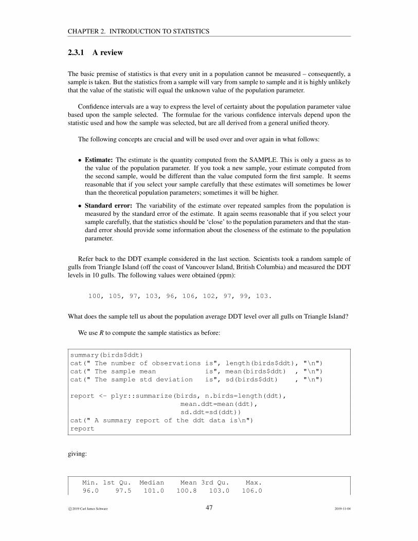
Scientists took a random sample (how was this done?) of 10 gulls and found the following DDTlevels (ppm).
100, 105, 97, 103, 96, 106, 102, 97, 99, 103.
The data is available in the ddt.csv file in the Sample Program Library at http://www.stat.sfu.ca/~cschwarz/Stat-Ecology-Datasets. The data are imported into R using the read.csv()function:
birds <- read.csv("ddt.csv", header=TRUE, as.is=TRUE)birds
The raw data are shown below:
ddt sex mass1 100 m 1750
c©2019 Carl James Schwarz 39 2019-11-04
CHAPTER 2. INTRODUCTION TO STATISTICS
2 105 m 15003 97 m 18504 103 m 17005 96 m 18006 106 f 16507 102 f 16008 97 f 15509 99 f 160010 103 f 1750
Sample mean and sample standard deviation The sample average and sample standard deviationcould be computed from these value using a spreadsheet, calculator, or a statistical package.
We begin by obtaining some basic plots of the data to get a feel for the general shape of the distribu-tion of data values, check for outliers, etc.
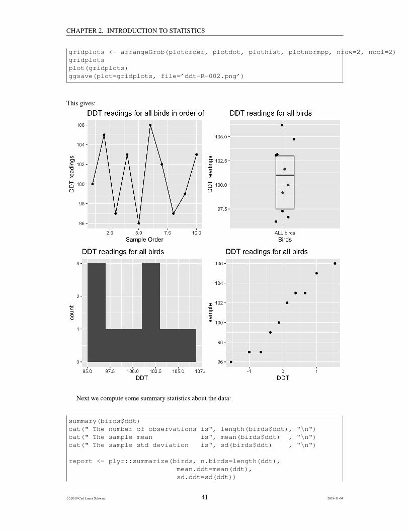
# Do some preliminary plots# With only a few data points the plots are not that# interesting. This also illustrates how to arrange# several plots into a grid and how to# save plots to an external file
# A time plot of reading over the order collectedplotorder <- ggplot(data=birds, aes(x=1:length(ddt), y=ddt))+
ggtitle("DDT readings for all birds in order of collection")+xlab("Sample Order")+ylab("DDT readings")+geom_point()+geom_line()
plotorder
# A regular dot plot with a box plot overlaidplotdot <- ggplot(data=birds, aes(x="ALL birds", y=ddt))+
ggtitle("DDT readings for all birds")+xlab("Birds")+ylab("DDT readings")+geom_point(position=position_jitter(w=0.1))+geom_boxplot(alpha=0.2, width=0.2)
plotdot
# A (non-interesting) histogramplothist <- ggplot(data=birds, aes(x=ddt))+
ggtitle("DDT readings for all birds")+xlab("DDT")+geom_histogram(binwidth=2)
plothist
# A normal probability plot - note how the aes() changesplotnormpp <- ggplot(data=birds, aes(sample=ddt))+
ggtitle("DDT readings for all birds")+xlab("DDT")+stat_qq()
plotnormpp
# Put them together into one big plot
c©2019 Carl James Schwarz 40 2019-11-04
CHAPTER 2. INTRODUCTION TO STATISTICS
gridplots <- arrangeGrob(plotorder, plotdot, plothist, plotnormpp, nrow=2, ncol=2)gridplotsplot(gridplots)ggsave(plot=gridplots, file=’ddt-R-002.png’)
This gives:
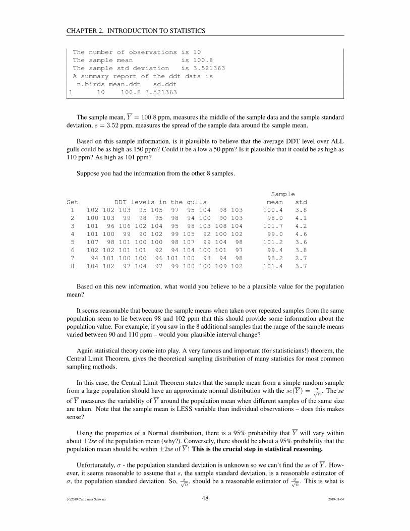
Next we compute some summary statistics about the data:
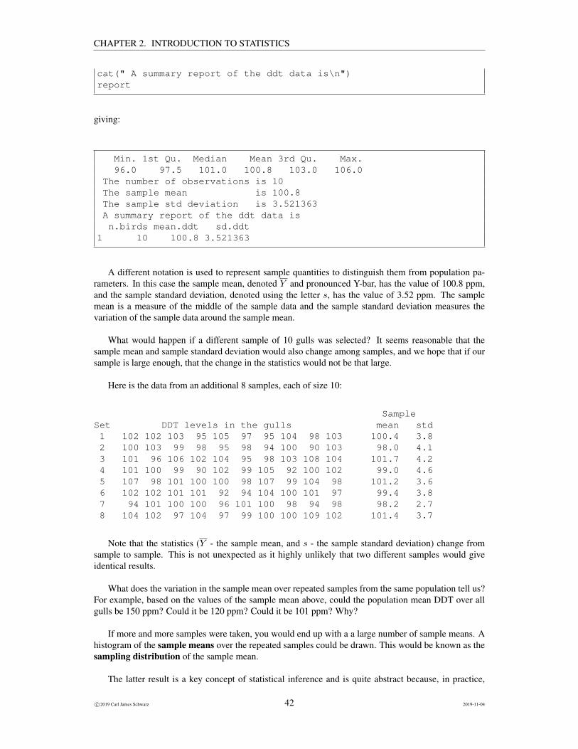
summary(birds$ddt)cat(" The number of observations is", length(birds$ddt), "\n")cat(" The sample mean is", mean(birds$ddt) , "\n")cat(" The sample std deviation is", sd(birds$ddt) , "\n")
report <- plyr::summarize(birds, n.birds=length(ddt),mean.ddt=mean(ddt),sd.ddt=sd(ddt))
c©2019 Carl James Schwarz 41 2019-11-04
CHAPTER 2. INTRODUCTION TO STATISTICS
cat(" A summary report of the ddt data is\n")report
giving:
Min. 1st Qu. Median Mean 3rd Qu. Max.96.0 97.5 101.0 100.8 103.0 106.0
The number of observations is 10The sample mean is 100.8The sample std deviation is 3.521363A summary report of the ddt data isn.birds mean.ddt sd.ddt
1 10 100.8 3.521363
A different notation is used to represent sample quantities to distinguish them from population pa-rameters. In this case the sample mean, denoted Y and pronounced Y-bar, has the value of 100.8 ppm,and the sample standard deviation, denoted using the letter s, has the value of 3.52 ppm. The samplemean is a measure of the middle of the sample data and the sample standard deviation measures thevariation of the sample data around the sample mean.
What would happen if a different sample of 10 gulls was selected? It seems reasonable that thesample mean and sample standard deviation would also change among samples, and we hope that if oursample is large enough, that the change in the statistics would not be that large.
Here is the data from an additional 8 samples, each of size 10:
SampleSet DDT levels in the gulls mean std1 102 102 103 95 105 97 95 104 98 103 100.4 3.82 100 103 99 98 95 98 94 100 90 103 98.0 4.13 101 96 106 102 104 95 98 103 108 104 101.7 4.24 101 100 99 90 102 99 105 92 100 102 99.0 4.65 107 98 101 100 100 98 107 99 104 98 101.2 3.66 102 102 101 101 92 94 104 100 101 97 99.4 3.87 94 101 100 100 96 101 100 98 94 98 98.2 2.78 104 102 97 104 97 99 100 100 109 102 101.4 3.7
Note that the statistics (Y - the sample mean, and s - the sample standard deviation) change fromsample to sample. This is not unexpected as it highly unlikely that two different samples would giveidentical results.
What does the variation in the sample mean over repeated samples from the same population tell us?For example, based on the values of the sample mean above, could the population mean DDT over allgulls be 150 ppm? Could it be 120 ppm? Could it be 101 ppm? Why?
If more and more samples were taken, you would end up with a a large number of sample means. Ahistogram of the sample means over the repeated samples could be drawn. This would be known as thesampling distribution of the sample mean.
The latter result is a key concept of statistical inference and is quite abstract because, in practice,
c©2019 Carl James Schwarz 42 2019-11-04
CHAPTER 2. INTRODUCTION TO STATISTICS
you never see the sampling distribution. The distribution of individual values over the entire populationcan be visualized; the distribution of individual values in the particular sample can be examined directlyas you have actual data; the hypothetical distribution of a statistics over repeated samples from thepopulation is always present, but remains one level of abstraction away from the actual data.
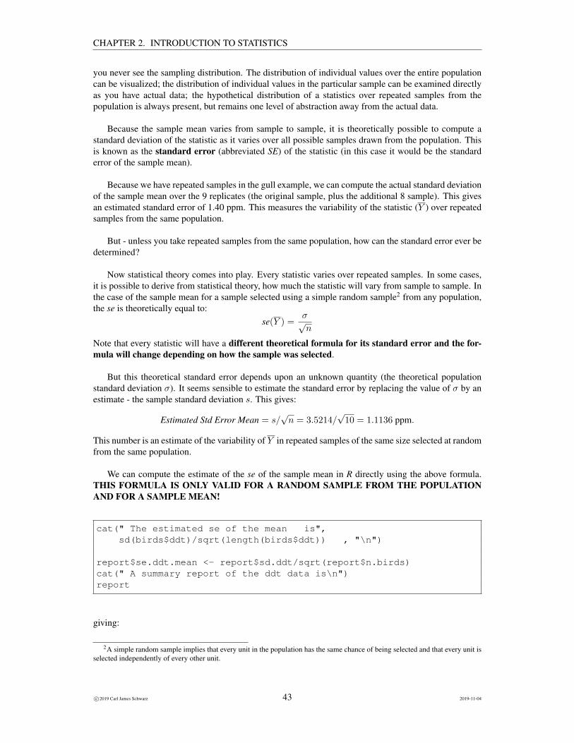
Because the sample mean varies from sample to sample, it is theoretically possible to compute astandard deviation of the statistic as it varies over all possible samples drawn from the population. Thisis known as the standard error (abbreviated SE) of the statistic (in this case it would be the standarderror of the sample mean).
Because we have repeated samples in the gull example, we can compute the actual standard deviationof the sample mean over the 9 replicates (the original sample, plus the additional 8 sample). This givesan estimated standard error of 1.40 ppm. This measures the variability of the statistic (Y ) over repeatedsamples from the same population.
But - unless you take repeated samples from the same population, how can the standard error ever bedetermined?
Now statistical theory comes into play. Every statistic varies over repeated samples. In some cases,it is possible to derive from statistical theory, how much the statistic will vary from sample to sample. Inthe case of the sample mean for a sample selected using a simple random sample2 from any population,the se is theoretically equal to:
se(Y ) =σ√n
Note that every statistic will have a different theoretical formula for its standard error and the for-mula will change depending on how the sample was selected.
But this theoretical standard error depends upon an unknown quantity (the theoretical populationstandard deviation σ). It seems sensible to estimate the standard error by replacing the value of σ by anestimate - the sample standard deviation s. This gives:
Estimated Std Error Mean = s/√n = 3.5214/
√10 = 1.1136 ppm.
This number is an estimate of the variability of Y in repeated samples of the same size selected at randomfrom the same population.
We can compute the estimate of the se of the sample mean in R directly using the above formula.THIS FORMULA IS ONLY VALID FOR A RANDOM SAMPLE FROM THE POPULATIONAND FOR A SAMPLE MEAN!
cat(" The estimated se of the mean is",sd(birds$ddt)/sqrt(length(birds$ddt)) , "\n")
report$se.ddt.mean <- report$sd.ddt/sqrt(report$n.birds)cat(" A summary report of the ddt data is\n")report
giving:
2A simple random sample implies that every unit in the population has the same chance of being selected and that every unit isselected independently of every other unit.
c©2019 Carl James Schwarz 43 2019-11-04

CHAPTER 2. INTRODUCTION TO STATISTICS
The estimated se of the mean is 1.113553A summary report of the ddt data isn.birds mean.ddt sd.ddt se.ddt.mean
1 10 100.8 3.521363 1.113553
A Summary of the crucial points:
• Parameter The parameter is a numerical measure of the entire population. Two common parame-ters are the population mean (denoted by µ) and the population standard deviation (denoted by σ).The population standard deviation measures the variation of individual values over all units in thepopulation. Parameters always refer to the population, never to the sample.
• Statistics or Estimate: A statistic or an estimate is a numerical quantity computed from the SAM-PLE. This is only a guess as to the value of the population parameter. If you took a new sample,your estimate computed from the second sample, would be different than the value computed formthe first sample. Two common statistics are the sample mean (denoted Y ), and the sample standarddeviation (denotes s). The sample standard deviation measures the variation of individual valuesover the units in the sample. Statistics always refer to the sample, never to the population.
• Sampling distribution Any statistic or estimate will change if a new sample is taken. The distri-bution of the statistic or estimate over repeated samples from the same population is known as thesampling distribution.
• Theoretical Standard error: The variability of the estimate over all possible repeated samplesfrom the population is measured by the standard error of the estimate. This is a theoretical quantityand could only be computed if you actually took all possible samples from the population.
• Estimated standard error Now for the hard part - you typically only take a single sample fromthe population. But, based upon statistical theory, you know the form of the theoretical standarderror, so you can use information from the sample to estimate the theoretical standard error. Becareful to distinguish between the standard deviation of individual values in your sample and theestimated standard error of the statistic as they refer to different types of variation. The formulafor the estimated standard error is different for every statistic and also depends upon the way thesample was selected. Consequently it is vitally important that the method of sample selectionand the type of estimate computed be determined carefully before using a computer packageto blindly compute standard errors.
The concept of a standard error is the MOST DIFFICULT CONCEPT to grasp in statistics. Thereason that it is so difficult, is that there is an extra layer of abstraction between what you observe andwhat is really happening. It is easy to visualize variation of individual elements in a sample because thevalues are there for you to see. It is easy to visualize variation of individual elements in a populationbecause you can picture the set of individual units. But it is difficult to visualize the set of all possiblesamples because typically you only take a single sample, and the set of all possible samples is so large.
As a final note, please do NOT use the ± notation for standard errors. The problem is that the ±notation is ambiguous and different papers in the same journal and different parts of the same paper usethe ± notation for different meanings. Modern usage is to write phrases such as “the estimated meanDDT level was 100.8 (SE 1.1) ppm.”
c©2019 Carl James Schwarz 44 2019-11-04
CHAPTER 2. INTRODUCTION TO STATISTICS
2.2.2 Theoretical example of a sampling distribution
Here is more detailed examination of a sampling distribution where the actual set of all possible samplescan be constructed. It shows that the sample mean is unbiased and that its standard error computed fromall possible samples matches that derived from statistical theory.
Suppose that a population consisted of five mice and we wish to estimate the average weight basedon a sample of size 2. [Obviously, the example is hopelessly simplified compared to a real populationand sampling experiment!]
Normally, the population values would not be known in advance (because then why would you haveto take a sample?). But suppose that the five mice had weights (in grams) of:
33, 28, 45, 43, 47.
The population mean weight and population standard deviation are found as:
• µ = (33+28+45+43+47) = 39.20 g, and
• σ = 7.39 g.
The population mean is the average weight over all possible units in the population. The populationstandard deviation measures the variation of individual weights about the mean, over the populationunits.
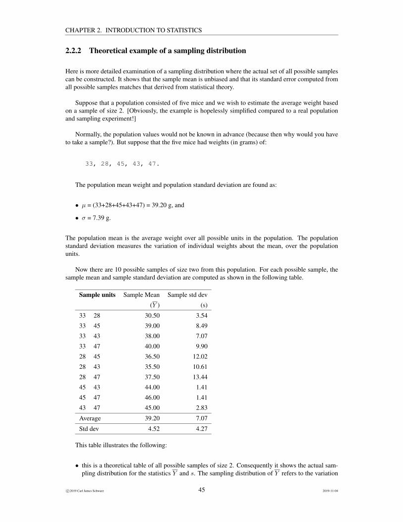
Now there are 10 possible samples of size two from this population. For each possible sample, thesample mean and sample standard deviation are computed as shown in the following table.
Sample units Sample Mean Sample std dev
(Y ) (s)
33 28 30.50 3.54
33 45 39.00 8.49
33 43 38.00 7.07
33 47 40.00 9.90
28 45 36.50 12.02
28 43 35.50 10.61
28 47 37.50 13.44
45 43 44.00 1.41
45 47 46.00 1.41
43 47 45.00 2.83
Average 39.20 7.07
Std dev 4.52 4.27
This table illustrates the following:
• this is a theoretical table of all possible samples of size 2. Consequently it shows the actual sam-pling distribution for the statistics Y and s. The sampling distribution of Y refers to the variation
c©2019 Carl James Schwarz 45 2019-11-04
CHAPTER 2. INTRODUCTION TO STATISTICS
of Y over all the possible samples from the population. Similarly, the sampling distribution of srefers to the variation of s over all possible samples from the population.
• some values of Y are above the population mean, and some values of Y are below the populationmean. We don’t know for any single sample if we are above or below the value of the populationparameter. Similarly, values of s (which is a sample standard deviation) also varies above andbelow the population standard deviation.
• the average (expected) value of Y over all possible samples is equal to the population mean. Wesay such estimators are unbiased. This is the hard concept! The extra level of abstraction is here- the statistic computed from an individual sample, has a distribution over all possible samples,hence the sampling distribution.
• the average (expected) value of s over all possible samples is NOT equal to the population standarddeviation. We say that s is a biased estimator. This is a difficult concept - you are taking theaverage of an estimate of the standard deviation. The average is taken over possible values of sfrom all possible samples. The latter is an extra level of abstraction from the raw data. [There isnothing theoretically wrong with using a biased estimator, but most people would prefer to use anunbiased estimator. It turns out that the bias in s decreases very rapidly with sample size and so isnot a concern.]
• the standard deviation of Y refers to the variation of Y over all possible samples. We call this thestandard error of a statistic. [The term comes from an historical context that is not important atthis point.]. Do not confuse the standard error of a statistic with the sample standard deviation orthe population standard deviation. The standard error measures the variability of a statistic (e.g.Y ) over all possible samples. The sample standard deviation measures variability of individualunits in the sample. The population standard deviation measures variability of individual units inthe population.
• if the previous formula for the theoretical standard error was used in this example it would fail togive the correct answer:
i.e. se(Y ) = 4.52 6= σ√n
= 7.39√2
= 5.22 The reason that this formulae didn’t work is that thesample size was an appreciable fraction of the entire population. A finite population correctionneeds to be applied in these cases. As you will see in later chapters, the se in this case is computedas:
se(Y ) =σ√n
√(1− f)
√N
(N − 1)=
7.39√2
√(1− 2
5
√5
4= 4.52
Refer to the chapter on survey sampling for more details.
2.3 Confidence Intervals
Section summary:
1. Understand the general logic of why a confidence interval works.
2. How to graph a confidence interval for a single parameter.
3. How to interpret graphs of several confidence intervals.
4. Effect of sample size upon the size of a confidence interval.
5. Effect of variability upon the size of a confidence interval.
6. Effect of confidence level upon the size of a confidence interval.
c©2019 Carl James Schwarz 46 2019-11-04
CHAPTER 2. INTRODUCTION TO STATISTICS
2.3.1 A review
The basic premise of statistics is that every unit in a population cannot be measured – consequently, asample is taken. But the statistics from a sample will vary from sample to sample and it is highly unlikelythat the value of the statistic will equal the unknown value of the population parameter.
Confidence intervals are a way to express the level of certainty about the population parameter valuebased upon the sample selected. The formulae for the various confidence intervals depend upon thestatistic used and how the sample was selected, but are all derived from a general unified theory.
The following concepts are crucial and will be used over and over again in what follows:
• Estimate: The estimate is the quantity computed from the SAMPLE. This is only a guess as tothe value of the population parameter. If you took a new sample, your estimate computed fromthe second sample, would be different than the value computed form the first sample. It seemsreasonable that if you select your sample carefully that these estimates will sometimes be lowerthan the theoretical population parameters; sometimes it will be higher.
• Standard error: The variability of the estimate over repeated samples from the population ismeasured by the standard error of the estimate. It again seems reasonable that if you select yoursample carefully, that the statistics should be ‘close’ to the population parameters and that the stan-dard error should provide some information about the closeness of the estimate to the populationparameter.
Refer back to the DDT example considered in the last section. Scientists took a random sample ofgulls from Triangle Island (off the coast of Vancouver Island, British Columbia) and measured the DDTlevels in 10 gulls. The following values were obtained (ppm):
100, 105, 97, 103, 96, 106, 102, 97, 99, 103.
What does the sample tell us about the population average DDT level over all gulls on Triangle Island?
We use R to compute the sample statistics as before:
summary(birds$ddt)cat(" The number of observations is", length(birds$ddt), "\n")cat(" The sample mean is", mean(birds$ddt) , "\n")cat(" The sample std deviation is", sd(birds$ddt) , "\n")
report <- plyr::summarize(birds, n.birds=length(ddt),mean.ddt=mean(ddt),sd.ddt=sd(ddt))
cat(" A summary report of the ddt data is\n")report
giving:
Min. 1st Qu. Median Mean 3rd Qu. Max.96.0 97.5 101.0 100.8 103.0 106.0
c©2019 Carl James Schwarz 47 2019-11-04
CHAPTER 2. INTRODUCTION TO STATISTICS
The number of observations is 10The sample mean is 100.8The sample std deviation is 3.521363A summary report of the ddt data isn.birds mean.ddt sd.ddt
1 10 100.8 3.521363
The sample mean, Y = 100.8 ppm, measures the middle of the sample data and the sample standarddeviation, s = 3.52 ppm, measures the spread of the sample data around the sample mean.
Based on this sample information, is it plausible to believe that the average DDT level over ALLgulls could be as high as 150 ppm? Could it be a low a 50 ppm? Is it plausible that it could be as high as110 ppm? As high as 101 ppm?
Suppose you had the information from the other 8 samples.
SampleSet DDT levels in the gulls mean std1 102 102 103 95 105 97 95 104 98 103 100.4 3.82 100 103 99 98 95 98 94 100 90 103 98.0 4.13 101 96 106 102 104 95 98 103 108 104 101.7 4.24 101 100 99 90 102 99 105 92 100 102 99.0 4.65 107 98 101 100 100 98 107 99 104 98 101.2 3.66 102 102 101 101 92 94 104 100 101 97 99.4 3.87 94 101 100 100 96 101 100 98 94 98 98.2 2.78 104 102 97 104 97 99 100 100 109 102 101.4 3.7
Based on this new information, what would you believe to be a plausible value for the populationmean?
It seems reasonable that because the sample means when taken over repeated samples from the samepopulation seem to lie between 98 and 102 ppm that this should provide some information about thepopulation value. For example, if you saw in the 8 additional samples that the range of the sample meansvaried between 90 and 110 ppm – would your plausible interval change?
Again statistical theory come into play. A very famous and important (for statisticians!) theorem, theCentral Limit Theorem, gives the theoretical sampling distribution of many statistics for most commonsampling methods.
In this case, the Central Limit Theorem states that the sample mean from a simple random samplefrom a large population should have an approximate normal distribution with the se(Y ) = σ√
n. The se
of Y measures the variability of Y around the population mean when different samples of the same sizeare taken. Note that the sample mean is LESS variable than individual observations – does this makessense?
Using the properties of a Normal distribution, there is a 95% probability that Y will vary withinabout±2se of the population mean (why?). Conversely, there should be about a 95% probability that thepopulation mean should be within ±2se of Y ! This is the crucial step in statistical reasoning.
Unfortunately, σ - the population standard deviation is unknown so we can’t find the se of Y . How-ever, it seems reasonable to assume that s, the sample standard deviation, is a reasonable estimator ofσ, the population standard deviation. So, s√
n, should be a reasonable estimator of σ√
n. This is what is
c©2019 Carl James Schwarz 48 2019-11-04
CHAPTER 2. INTRODUCTION TO STATISTICS
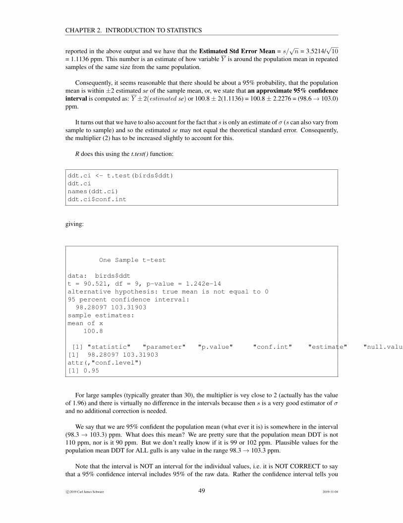
reported in the above output and we have that the Estimated Std Error Mean = s/√n = 3.5214/
√10
= 1.1136 ppm. This number is an estimate of how variable Y is around the population mean in repeatedsamples of the same size from the same population.
Consequently, it seems reasonable that there should be about a 95% probability, that the populationmean is within ±2 estimated se of the sample mean, or, we state that an approximate 95% confidenceinterval is computed as: Y ±2(estimated se) or 100.8± 2(1.1136) = 100.8± 2.2276 = (98.6→ 103.0)ppm.
It turns out that we have to also account for the fact that s is only an estimate of σ (s can also vary fromsample to sample) and so the estimated se may not equal the theoretical standard error. Consequently,the multiplier (2) has to be increased slightly to account for this.
R does this using the t.test() function:
ddt.ci <- t.test(birds$ddt)ddt.cinames(ddt.ci)ddt.ci$conf.int
giving:
One Sample t-test
data: birds$ddtt = 90.521, df = 9, p-value = 1.242e-14alternative hypothesis: true mean is not equal to 095 percent confidence interval:
98.28097 103.31903sample estimates:mean of x
100.8
[1] "statistic" "parameter" "p.value" "conf.int" "estimate" "null.value" "stderr" "alternative" "method" "data.name"[1] 98.28097 103.31903attr(,"conf.level")[1] 0.95
For large samples (typically greater than 30), the multiplier is vey close to 2 (actually has the valueof 1.96) and there is virtually no difference in the intervals because then s is a very good estimator of σand no additional correction is needed.
We say that we are 95% confident the population mean (what ever it is) is somewhere in the interval(98.3 → 103.3) ppm. What does this mean? We are pretty sure that the population mean DDT is not110 ppm, nor is it 90 ppm. But we don’t really know if it is 99 or 102 ppm. Plausible values for thepopulation mean DDT for ALL gulls is any value in the range 98.3→ 103.3 ppm.
Note that the interval is NOT an interval for the individual values, i.e. it is NOT CORRECT to saythat a 95% confidence interval includes 95% of the raw data. Rather the confidence interval tells you
c©2019 Carl James Schwarz 49 2019-11-04
CHAPTER 2. INTRODUCTION TO STATISTICS
a plausible range for the population mean µ. Also, it is not a confidence interval for the sample mean(which you know to be 100.8) but rather for the unknown population mean µ. These two points are themost common mis-interpretations of confidence intervals.
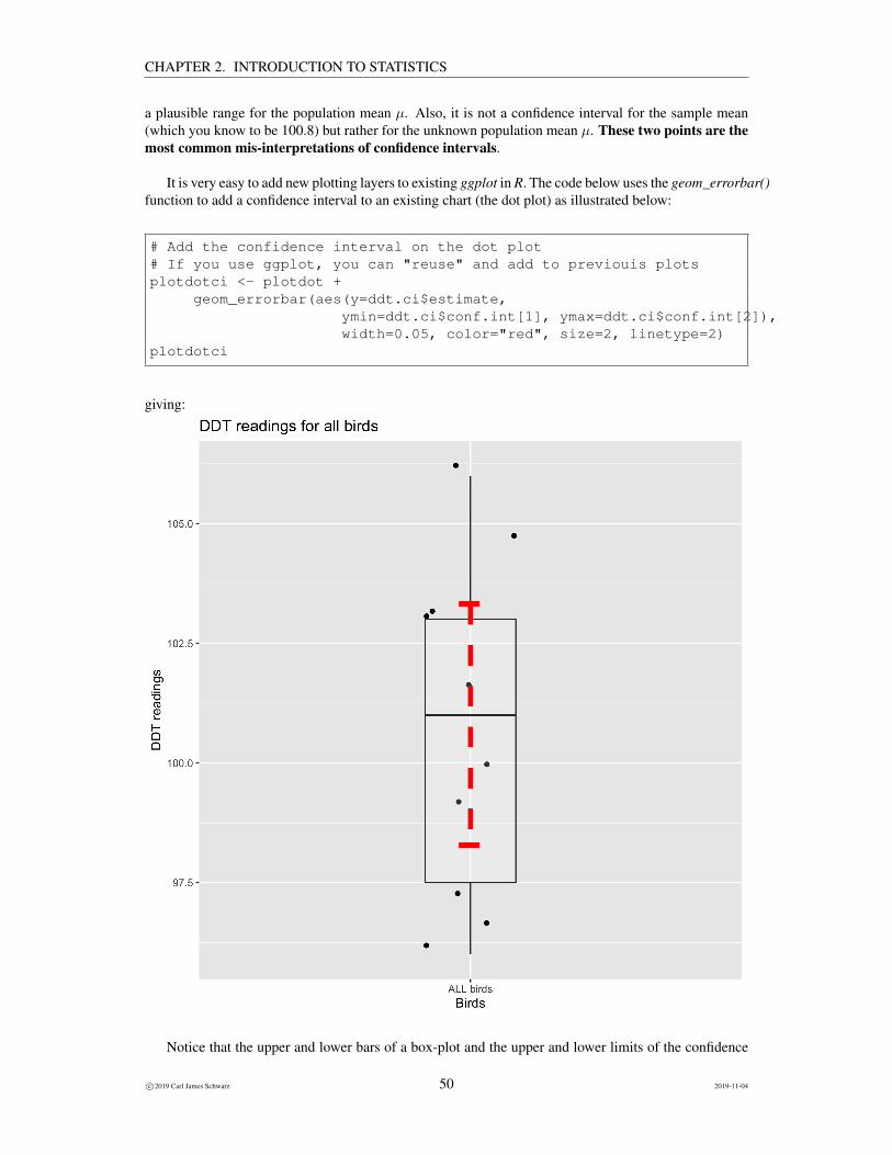
It is very easy to add new plotting layers to existing ggplot in R. The code below uses the geom_errorbar()function to add a confidence interval to an existing chart (the dot plot) as illustrated below:
# Add the confidence interval on the dot plot# If you use ggplot, you can "reuse" and add to previouis plotsplotdotci <- plotdot +
geom_errorbar(aes(y=ddt.ci$estimate,ymin=ddt.ci$conf.int[1], ymax=ddt.ci$conf.int[2]),width=0.05, color="red", size=2, linetype=2)
plotdotci
giving:
Notice that the upper and lower bars of a box-plot and the upper and lower limits of the confidence
c©2019 Carl James Schwarz 50 2019-11-04
CHAPTER 2. INTRODUCTION TO STATISTICS
intervals are telling you different stories. Be sure that you understand the difference!
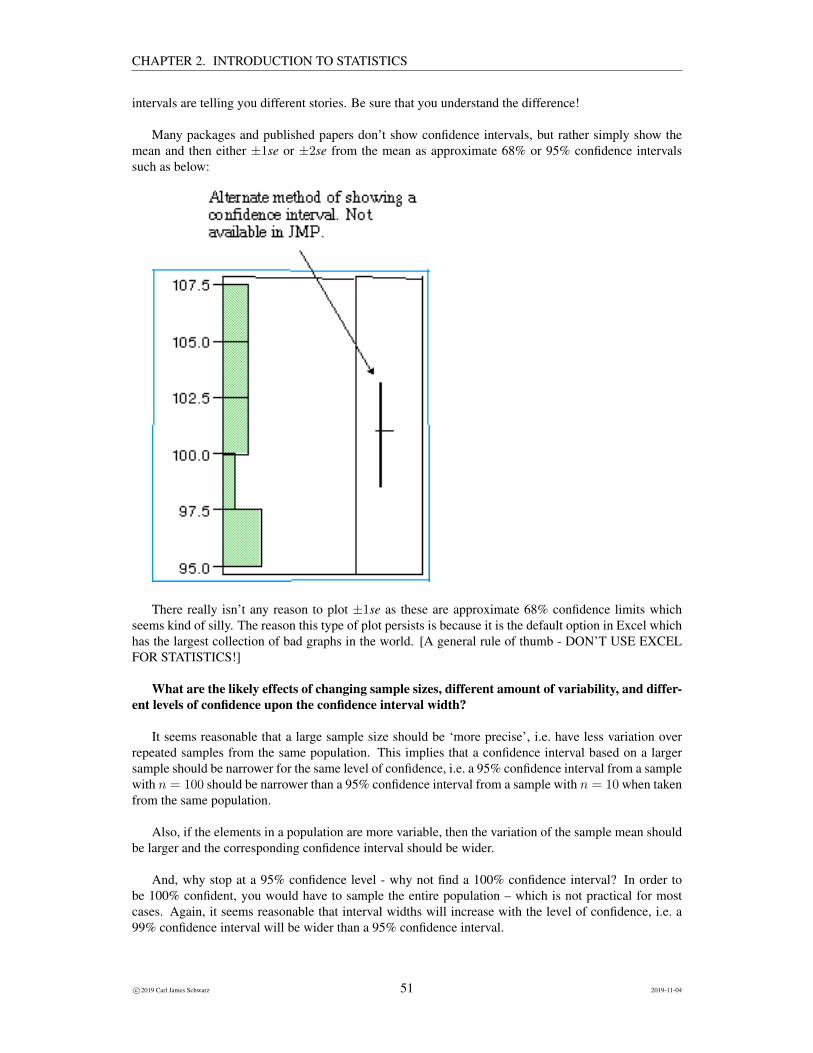
Many packages and published papers don’t show confidence intervals, but rather simply show themean and then either ±1se or ±2se from the mean as approximate 68% or 95% confidence intervalssuch as below:
There really isn’t any reason to plot ±1se as these are approximate 68% confidence limits whichseems kind of silly. The reason this type of plot persists is because it is the default option in Excel whichhas the largest collection of bad graphs in the world. [A general rule of thumb - DON’T USE EXCELFOR STATISTICS!]
What are the likely effects of changing sample sizes, different amount of variability, and differ-ent levels of confidence upon the confidence interval width?
It seems reasonable that a large sample size should be ‘more precise’, i.e. have less variation overrepeated samples from the same population. This implies that a confidence interval based on a largersample should be narrower for the same level of confidence, i.e. a 95% confidence interval from a samplewith n = 100 should be narrower than a 95% confidence interval from a sample with n = 10 when takenfrom the same population.
Also, if the elements in a population are more variable, then the variation of the sample mean shouldbe larger and the corresponding confidence interval should be wider.
And, why stop at a 95% confidence level - why not find a 100% confidence interval? In order tobe 100% confident, you would have to sample the entire population – which is not practical for mostcases. Again, it seems reasonable that interval widths will increase with the level of confidence, i.e. a99% confidence interval will be wider than a 95% confidence interval.
c©2019 Carl James Schwarz 51 2019-11-04
CHAPTER 2. INTRODUCTION TO STATISTICS
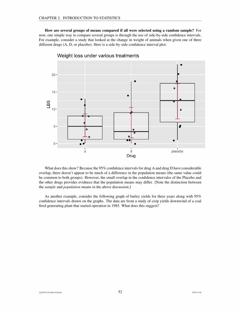
How are several groups of means compared if all were selected using a random sample? Fornow, one simple way to compare several groups is through the use of side-by-side confidence intervals.For example, consider a study that looked at the change in weight of animals when given one of threedifferent drugs (A, D, or placebo). Here is a side-by-side confidence interval plot:
What does this show? Because the 95% confidence intervals for drug A and drug D have considerableoverlap, there doesn’t appear to be much of a difference in the population means (the same value couldbe common to both groups). However, the small overlap in the confidence intervalss of the Placebo andthe other drugs provides evidnece that the population means may differ. [Note the distinction betweenthe sample and population means in the above discussion.]
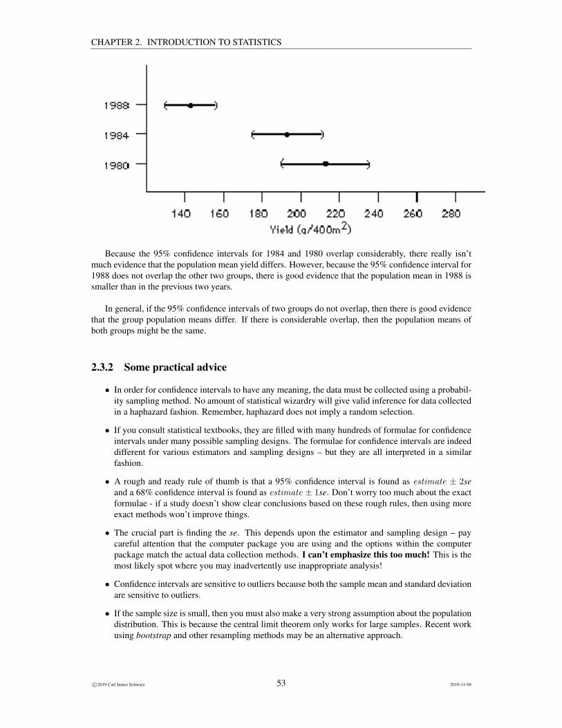
As another example, consider the following graph of barley yields for three years along with 95%confidence intervals drawn on the graphs. The data are from a study of crop yields downwind of a coalfired generating plant that started operation in 1985. What does this suggest?
c©2019 Carl James Schwarz 52 2019-11-04
CHAPTER 2. INTRODUCTION TO STATISTICS
Because the 95% confidence intervals for 1984 and 1980 overlap considerably, there really isn’tmuch evidence that the population mean yield differs. However, because the 95% confidence interval for1988 does not overlap the other two groups, there is good evidence that the population mean in 1988 issmaller than in the previous two years.
In general, if the 95% confidence intervals of two groups do not overlap, then there is good evidencethat the group population means differ. If there is considerable overlap, then the population means ofboth groups might be the same.
2.3.2 Some practical advice
• In order for confidence intervals to have any meaning, the data must be collected using a probabil-ity sampling method. No amount of statistical wizardry will give valid inference for data collectedin a haphazard fashion. Remember, haphazard does not imply a random selection.
• If you consult statistical textbooks, they are filled with many hundreds of formulae for confidenceintervals under many possible sampling designs. The formulae for confidence intervals are indeeddifferent for various estimators and sampling designs – but they are all interpreted in a similarfashion.
• A rough and ready rule of thumb is that a 95% confidence interval is found as estimate ± 2seand a 68% confidence interval is found as estimate ± 1se. Don’t worry too much about the exactformulae - if a study doesn’t show clear conclusions based on these rough rules, then using moreexact methods won’t improve things.
• The crucial part is finding the se. This depends upon the estimator and sampling design – paycareful attention that the computer package you are using and the options within the computerpackage match the actual data collection methods. I can’t emphasize this too much! This is themost likely spot where you may inadvertently use inappropriate analysis!
• Confidence intervals are sensitive to outliers because both the sample mean and standard deviationare sensitive to outliers.
• If the sample size is small, then you must also make a very strong assumption about the populationdistribution. This is because the central limit theorem only works for large samples. Recent workusing bootstrap and other resampling methods may be an alternative approach.
c©2019 Carl James Schwarz 53 2019-11-04
CHAPTER 2. INTRODUCTION TO STATISTICS
• The confidence interval only tells you the uncertainty in knowing the population parameterbecause you only measured a sample from the population3. It does not cover potential impreci-sion caused by nonresponse, under-coverage, measurement errors etc. In many cases, these can beorders of magnitude larger - particularly if the data was not collected according to a well definedplan.
2.3.3 Technical details
The formula for a confidence interval for a single mean when the data are collected using a simplerandom sample from a population with normally distributed data is:
Y ± tn−1 × se
orY ± tn−1
s√n
where the tn−1 refers to values from a t-distribution with (n − 1) degrees of freedom. Values ofthe t-distribution are tabulated in the tables located at http://www.stat.sfu.ca/~cschwarz/CourseNotes/. For the above example for gulls on Triangle Island, n = 10, so the multiplier for a95% confidence interval is t9 = 2.2622 and the confidence interval was found as: 100.8±2.262(1.1136) =100.8± 2.5192 = (98.28→ 103.32) ppm which matches the results provided by JMP.
Note that different sampling schemes may not use a t-distribution and most certainly will have dif-ferent degrees of freedom for the t-distribution.
This formula is useful when the raw data is not given, and only the summary statistics (typically thesample size, the sample mean, and the sample standard deviation) are given and a confidence intervalneeds to be computed.
What is the effect of sample size? If the above formula is examined, the primary place wherethe sample size n comes into play is the denominator of the standard error. So as n increases, the sedecreases. However note that the se decreases as a function of
√n, i.e. it takes 4× the sample size
to reduce the standard error by a factor of 2. This is sensible because as the sample size increases, Yshould be less variable (and usually closer to the population mean). Consequently, the width of theinterval decreases. The confidence level doesn’t change - we would still be roughly 95% confident, butthe interval is smaller. The sample size also affects the degrees of freedom which affects the t-value, butthis effect is minor compared to that change in the se.
What is the effect of increasing the confidence level? If you wanted to be 99% confident, thet-value from the table increases. For example, the t-value for 9 degrees of freedom increases from 2.262for a 95% confidence interval to 3.25 for a 99% confidence interval. In general, a higher confidence levelwill give a wider confidence interval.
2.4 Hypothesis testing
Section summary:
1. Understand the basic paradigm of hypothesis testing.
3This is technically known as the sampling error
c©2019 Carl James Schwarz 54 2019-11-04
CHAPTER 2. INTRODUCTION TO STATISTICS
2. Interpret p-values correctly.
3. Understand Type I, Type II, and Type III errors.
4. Understand the limitation of hypothesis testing.
2.4.1 A review
Hypothesis testing is an important paradigm of Statistical Inference, but has its limitations. In recentyears, emphasis has moved away from formal hypothesis testing to more inferential statistics (e.g. con-fidence intervals) but hypothesis testing still has an important role to play.
There are two common hypothesis testing situations encountered in ecology:
• Comparing the population parameter against a known standard. For example, environmental reg-ulations may specify that the mean contaminant loading in water must be less than a certain fixedvalue.
• Comparing the population parameter among 2 or more groups. For example, is the average DDTloading the same for males and female birds.
The key steps in hypothesis testing are:
• Formulate the hypothesis of NO CHANGE in terms of POPULATION parameters.
• Collect data using a good sampling design or a good experimental design paying careful attentionto the RRRs.
• Using the data, compute the difference between the sample estimate and the standard value, or thedifference in the sample estimates among the groups. A measure of precision is also needed, i.e. astandard error or a confidence interval.
• Evaluate if the observed change (or difference) is consistent with NO EFFECT. This is usuallysummarized by a p-value.
2.4.2 Comparing the population parameter against a known standard
Again consider the example of gulls on Triangle Island introduced in previous sections.
Of interest is the population mean DDT level over ALL the gulls. Let (µ) represent the average DDTover all gulls on the island. The value of this population parameter is unknown because you would haveto measure ALL gulls which is logistically impossible to do.
Now suppose that the value of 98 ppm is a critical value for the health of the species. Is there evidencethat the current population mean level is different than 98 ppm?
Scientists took a random sample (how was this done?) of 10 gulls and found the following DDTlevels.
100, 105, 97, 103, 96, 106, 102, 97, 99, 103.
c©2019 Carl James Schwarz 55 2019-11-04
CHAPTER 2. INTRODUCTION TO STATISTICS
We present the summary statistics computed by R previously:
Min. 1st Qu. Median Mean 3rd Qu. Max.96.0 97.5 101.0 100.8 103.0 106.0
The number of observations is 10The sample mean is 100.8The sample std deviation is 3.521363A summary report of the ddt data isn.birds mean.ddt sd.ddt
1 10 100.8 3.521363
One Sample t-test
data: birds$ddtt = 90.521, df = 9, p-value = 1.242e-14alternative hypothesis: true mean is not equal to 095 percent confidence interval:
98.28097 103.31903sample estimates:mean of x
100.8
[1] "statistic" "parameter" "p.value" "conf.int" "estimate" "null.value" "stderr" "alternative" "method" "data.name"[1] 98.28097 103.31903attr(,"conf.level")[1] 0.95
First examine the 95% confidence interval presented above. The confidence interval excludes thevalue of 98 ppm, so one is fairly confident that the population mean DDT level differs from 98 ppm.Furthermore the confidence interval gives information about what the population mean DDT level couldbe. Note that the hypothesized value of 98 ppm is just outside the 95% confidence interval.
A hypothesis test is much more ‘formal’ and consists of several steps:
1. Formulate hypothesis. This is a formal statement of two alternatives. The null hypothesis (de-noted as H0 or H) indicates the state of ignorance or no effect. The alternate hypothesis (denotedas H1 or A) indicates the effect that is to be detected if present.
Both the null and alternate hypothesis can be formulated before any data are collected and arealways formulated in terms of the population parameter. It is NEVER formulated in terms of thesample statistics as these would vary from sample to sample.
In this case, the null and alternate hypothesis are:
H:µ = 98, i.e. the mean DDT levels for ALL gulls is 98 ppm.
A:µ 6= 98, i.e. the mean DDT levels for ALL gulls is not 98 ppm.
This is known as a two-sided test because we are interested if the mean is either greater than orless than 98 ppm.4
4It is possible to construct what are known as one-sided tests where interest lies ONLY if the population mean exceeds 98 ppm,or a test if interest lies ONLY if the population mean is less than 98 ppm. These are rarely useful in ecological work.
c©2019 Carl James Schwarz 56 2019-11-04
CHAPTER 2. INTRODUCTION TO STATISTICS
2. Collect data. Again it is important that the data be collected using probability sampling methodsand the RRRs. The form of the data collection will influence the next step.
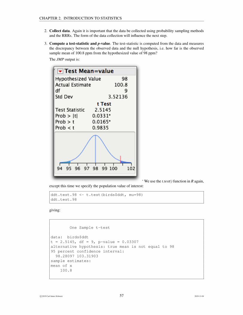
3. Compute a test-statistic and p-value. The test-statistic is computed from the data and measuresthe discrepancy between the observed data and the null hypothesis, i.e. how far is the observedsample mean of 100.8 ppm from the hypothesized value of 98 ppm?
The JMP output is:
‘ We use the t.test() function in R again,except this time we specify the population value of interest:
ddt.test.98 <- t.test(birds$ddt, mu=98)ddt.test.98
giving:
One Sample t-test
data: birds$ddtt = 2.5145, df = 9, p-value = 0.03307alternative hypothesis: true mean is not equal to 9895 percent confidence interval:
98.28097 103.31903sample estimates:mean of x
100.8
c©2019 Carl James Schwarz 57 2019-11-04
CHAPTER 2. INTRODUCTION TO STATISTICS
The output examines if the data are consistent with the hypothesized value (98 ppm) followed bythe estimate (the sample mean) of 100.8 ppm. From the earlier output, we know that the se of thesample mean is 1.11. R reports the confidence interval but not the standard error of the mean. Inmy opinion, this should always be reported.
How discordant is the sample mean of 100.8 ppm with the hypothesized value of 98 ppm? Onediscrepancy measure is known as a T-ratio and is computed as:
T =(estimate − hypothesized value)
estimated se=
(100.8− 98)
3.52136/√
10= 2.5145
This implies the estimate is about 2.5 se different from the null hypothesis value of 98. This T-ratiois labelled as the Test Statistic in the output.
Note that there are many measures of discrepancy of the estimate with the null hypothesis - JMPalso provides a ‘non-parametric’ statistic suitable when the assumption of normality in the popu-lation may be suspect - this is not covered in this course.
How is this measure of discordance between the sample mean (100.8) and the hypothesized valueof 98 assessed? The unusualness of the test statistic is measured by finding the probability ofobserving the current test statistic assuming the null hypothesis is true. In other words, if thehypothesis were true (and the population mean is 98 ppm), what is the probability finding a samplemean of 100.8 ppm?5
This is denoted the p-value. Notice that the p-value is attached to the data - it measures theprobability of the sample mean given the hypothesis is true. Probabilities CANNOT be attachedto hypotheses - it would be incorrect to say that there is a 3% that the hypothesis is true. Thehypothesis is either true or false, it can’t be “partially” true!6
It is possible to obtain different “sided” hypothesis tests using the t.test() function by varying thealternative = c(“two.sided”, “less”, “greater”) argument to the function. The default is a two-sided test which results in the p-value of 0.0331.
4. Make a decision. How are the test statistic and p-value used? The basic paradigm of hypothesistesting is that unusual events provide evidence against the null hypothesis. Logically, rare events“shouldn’t happen” if the null hypothesis is true. This logic can be confusing! We will discuss itmore in class.
In our case, the p-value of 0.0331 indicates there is an approximate 3.3% chance of observing asample mean that differs from the hypothesized value of 98 if the null hypothesis were true.
Is this unusual? There are no fixed guidelines for the degree of unusualness expected beforedeclaring it to be unusual. Many people use a 5% cut-off value, i.e. if the p-value is less than 0.05,then this is evidence against the null hypothesis; if the p-value is greater than 0.05 then this notevidence against the null hypothesis. [This cut-off value is often called the α-level.] If we adoptthis cut-off value, then our observed p-value of 0.0331 is evidence against the null hypothesis andwe find that there is evidence that the population mean DDT level is different than 98 ppm.
The plot at the bottom of the output that is presented by JMP is helpful in trying to understand whatis going on. [No such equivalent plot is readily available in R or SAS.] It tries to give a measure of howunusual the sample mean of 100.8 is relative to the hypothesized value of 98. If the hypothesis weretrue, and the population mean was 98, then you would expect the sample means to be clustered aroundthe value of 98. The bell-shaped curve shows the distribution of the SAMPLE MEANS if repeated sam-ples are taken from the same population. It is centered over the population mean (98) with a variabilitymeasured by the se of 1.11. The small vertical tick mark just under the value of 101, represents the ob-served sample mean of 100.8. You can see that the observed sample mean of 100.8 is somewhat unusual
5In actual fact, the probability is computed of finding a value of 100.8 or more distant from the hypothesized value of 98. Thiswill be explained in more detail later in the notes.
6This is similar to asking a small child if they took a cookie. The truth is either “yes” or “no”, but often you will get theresponse of “maybe” which really doesn’t make much sense!
c©2019 Carl James Schwarz 58 2019-11-04
CHAPTER 2. INTRODUCTION TO STATISTICS
compared to the population value of 98. The shaded areas in the two tails represents the probability ofobserving the value of the sample mean so far away from the hypothesised value (in either direction) ifthe hypothesis were true and represents the p-value.
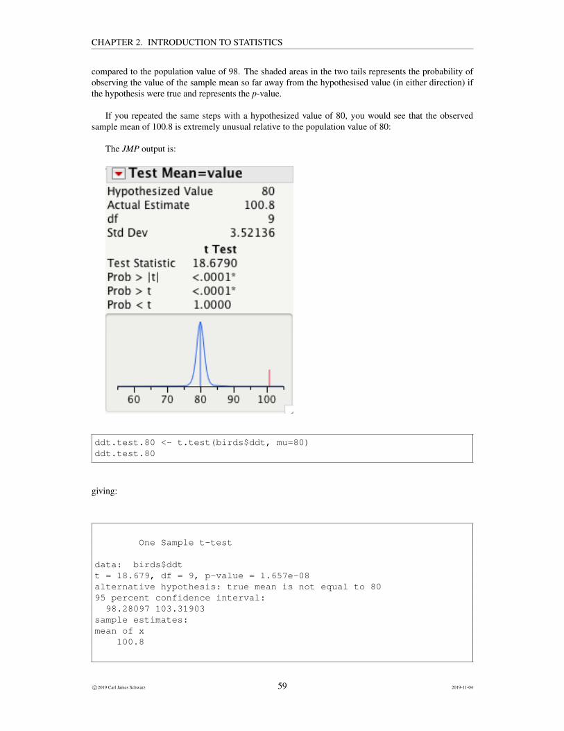
If you repeated the same steps with a hypothesized value of 80, you would see that the observedsample mean of 100.8 is extremely unusual relative to the population value of 80:
The JMP output is:
ddt.test.80 <- t.test(birds$ddt, mu=80)ddt.test.80
giving:
One Sample t-test
data: birds$ddtt = 18.679, df = 9, p-value = 1.657e-08alternative hypothesis: true mean is not equal to 8095 percent confidence interval:
98.28097 103.31903sample estimates:mean of x
100.8
c©2019 Carl James Schwarz 59 2019-11-04
CHAPTER 2. INTRODUCTION TO STATISTICS
The p-value is < .0001 indicating that the observed sample mean of 100.8 is very unusual relative to thehypothesis. We have evidence against the hypothesized value of 80.
Again, look at the graph produced by JMP. If the hypothesis were true, i.e. the population mean (µ)was 80 ppm, then you would expect to see most of the sample means clustered around the value of 80(the curve shown). The actual value of 100.8 is very unusual (if the hypothesis were true) – the verticaltick mark is so far from what would be expected.
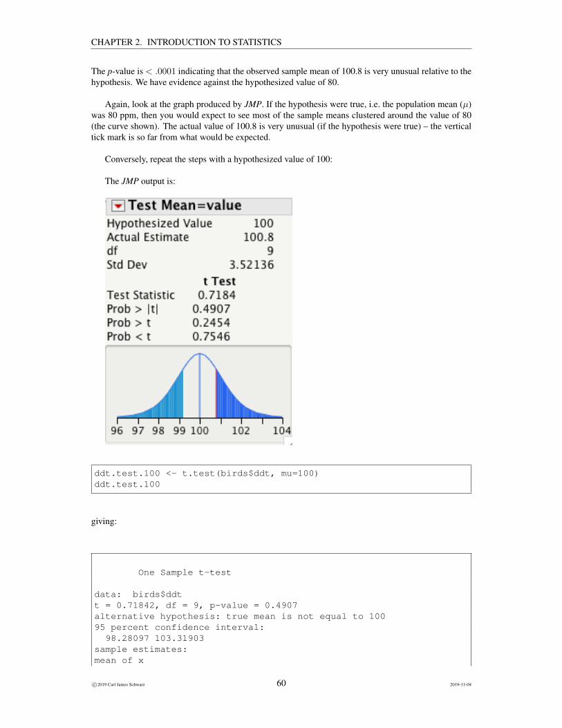
Conversely, repeat the steps with a hypothesized value of 100:
The JMP output is:
ddt.test.100 <- t.test(birds$ddt, mu=100)ddt.test.100
giving:
One Sample t-test
data: birds$ddtt = 0.71842, df = 9, p-value = 0.4907alternative hypothesis: true mean is not equal to 10095 percent confidence interval:
98.28097 103.31903sample estimates:mean of x
c©2019 Carl James Schwarz 60 2019-11-04
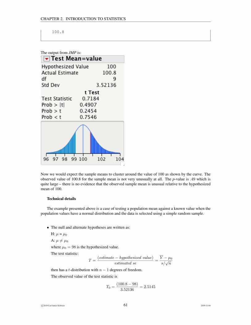
CHAPTER 2. INTRODUCTION TO STATISTICS
100.8
The output from JMP is:
Now we would expect the sample means to cluster around the value of 100 as shown by the curve. Theobserved value of 100.8 for the sample mean is not very unusually at all. The p-value is .49 which isquite large – there is no evidence that the observed sample mean is unusual relative to the hypothesizedmean of 100.
Technical details
The example presented above is a case of testing a population mean against a known value when thepopulation values have a normal distribution and the data is selected using a simple random sample.
• The null and alternate hypotheses are written as:
H: µ = µ0
A: µ 6= µ0
where µ0 = 98 is the hypothesized value.
The test statistic:
T =(estimate − hypothesized value)
estimated se=Y − µ0
s/√n
then has a t-distribution with n− 1 degrees of freedom.
The observed value of the test statistic is
T0 =(100.8− 98)
3.52136= 2.5145
c©2019 Carl James Schwarz 61 2019-11-04
CHAPTER 2. INTRODUCTION TO STATISTICS
The p-value is computed by finding
Prob(T > |T0|)
and is found to be 0.0331.
• In some very rare cases, the population standard deviation σ is known. In these cases, the standarderror is known, and the test statistic is compared to a normal distribution. This is extremely rare inpractise.
• The assumption of normality of the population values can be relaxed if the sample size is suffi-ciently large. In those cases, the central limit theorem indicates that the distribution of the test-statistics is known regardless of the underlying distribution of population values.
2.4.3 Comparing the population parameter between two groups
A common situation in ecology is to compare a population parameter in two (or more) groups. Forexample, it may be of interest to investigate if the mean DDT levels in males and females birds could bethe same.
There are now two population parameters of interest. The mean DDT level of male birds is denotedas µm while the mean DDT level of female birds is denoted as µf . These would be the mean DDT levelof all birds of their respective sex – once again this cannot be measured as not all birds can be sampled.
The hypotheses of interest are:
• H : µm = µf or H : µm − µf = 0
• A : µm 6= µf or H : µm − µf 6= 0
Again note that the hypotheses are in terms of the POPULATION parameters. The alternate hypothesisindicates that a difference in means in either direction is of interest, i.e. we don’t have an a prior beliefthat male birds have a smaller or larger population mean compared to female birds.
A random sample is taken from each of the populations using the RRR.
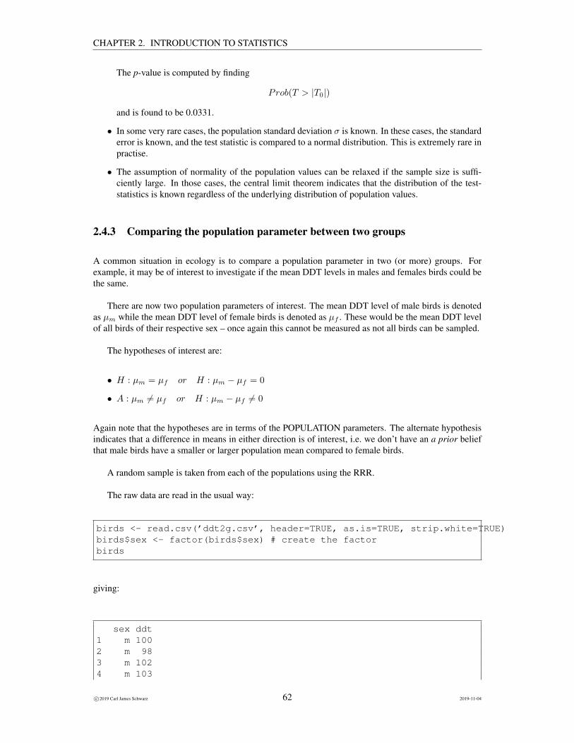
The raw data are read in the usual way:
birds <- read.csv(’ddt2g.csv’, header=TRUE, as.is=TRUE, strip.white=TRUE)birds$sex <- factor(birds$sex) # create the factorbirds
giving:
sex ddt1 m 1002 m 983 m 1024 m 103
c©2019 Carl James Schwarz 62 2019-11-04
CHAPTER 2. INTRODUCTION TO STATISTICS
5 m 996 f 1047 f 1058 f 1079 f 10510 f 103
Notice there are several columns - two of which are of interest. One column identifies the group mem-bership of each bird (the sex) and is nominal or ordinal in scale. The second column gives the DDTreading for each bird.7
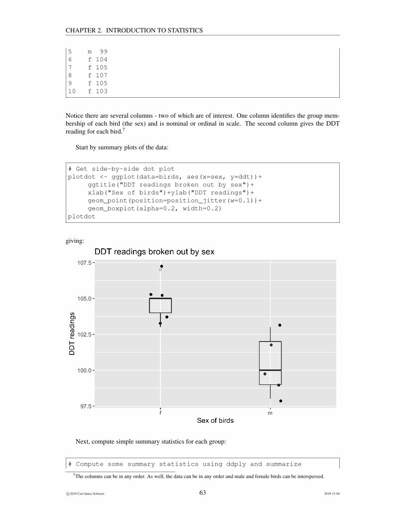
Start by summary plots of the data:
# Get side-by-side dot plotplotdot <- ggplot(data=birds, aes(x=sex, y=ddt))+
ggtitle("DDT readings broken out by sex")+xlab("Sex of birds")+ylab("DDT readings")+geom_point(position=position_jitter(w=0.1))+geom_boxplot(alpha=0.2, width=0.2)
plotdot
giving:
Next, compute simple summary statistics for each group:
# Compute some summary statistics using ddply and summarize
7The columns can be in any order. As well, the data can be in any order and male and female birds can be interspersed.
c©2019 Carl James Schwarz 63 2019-11-04
CHAPTER 2. INTRODUCTION TO STATISTICS
report <- plyr::ddply(birds, "sex", plyr::summarize,n.birds=length(ddt),mean.ddt = mean(ddt),sd.ddt = sd(ddt))
report# Compute some summary statistics by sex using my helper functionreport <- plyr::ddply(birds, "sex", sf.simple.summary, variable="ddt", crd=TRUE)report
giving:
sex n.birds mean.ddt sd.ddt1 f 5 104.8 1.4832402 m 5 100.4 2.073644
sex n nmiss mean sd se lcl ucl1 f 5 0 104.8 1.483240 0.6633250 102.95831 106.64172 m 5 0 100.4 2.073644 0.9273618 97.82523 102.9748
We also compute the 95% confidence intervals for each group:
ci <- plyr::ddply(birds, "sex", function(x){# compute the ci for the part of the dataframe xoneci <- t.test(x$ddt)$conf.intnames(oneci) <- c("lcl","ucl")return(oneci)
})ci
giving:
sex lcl ucl1 f 102.95831 106.64172 m 97.82523 102.9748
The individual sample means and se for each sex are reported along with 95% confidence intervals forthe population mean DDT of each sex. The 95% confidence intervals for the two sexes have virtually nooverlap which implies that a single plausible value common to both sexes is unlikely to exist.
Because we are interested in comparing the two population means, it seems sensible to estimate thedifference in the means. This can be done for this experiment using a statistical technique called (forhistorical reasons) a “t-test”8
result <- t.test(ddt ~ sex, data=birds)# compute the se
8The t-test requires a simple random sample from each group.
c©2019 Carl James Schwarz 64 2019-11-04

CHAPTER 2. INTRODUCTION TO STATISTICS
names(result)result$diff <- sum(result$estimate*c(1,-1))result$se <- abs(result$diff) /result$statisticresultcat("Estimated diff in MEANS is:", result$diff, " with an estimated SE ", result$se, "\n")
giving:
[1] "statistic" "parameter" "p.value" "conf.int" "estimate" "null.value" "stderr" "alternative" "method" "data.name"
Welch Two Sample t-test
data: ddt by sext = 3.8591, df = 7.2439, p-value = 0.005823alternative hypothesis: true difference in means is not equal to 095 percent confidence interval:1.722206 7.077794sample estimates:mean in group f mean in group m
104.8 100.4
Estimated diff in MEANS is: 4.4 with an estimated SE 1.140175
The first part of the output estimates the difference in the population means. Because each sam-ple mean is an unbiased estimator for the corresponding population mean, it seems reasonable that thedifference in sample means should be unbiased for the difference in population mean.
Unfortunately, many packages do NOT provide information on which order the difference in meanswas computed. Many packages order the groups alphabetically, but this can be often be changed. Theestimated difference in means is −4.4 ppm. The difference is negative indicating that the sample meanDDT for the males is less than the sample mean DDT for the females. As usual, a measure of precision(the se) should be reported for each estimate. The se for the difference in means is 1.14 (refer to laterchapters on how the se is computed), and the 95% confidence interval for the difference in populationmeans is from (−7.1 → −1.72). Because the 95% confidence interval for the difference in populationmeans does NOT include the value of 0, there is evidence that the mean DDT for all males could bedifferent than the mean DDT for all females.
The t ratio is again a measure of how far the difference in sample means is from the hypothesizedvalue of 0 difference and is found as the observed difference divided by the se of the difference. Thep-value of .0058 indicates that the observed difference in sample means of −4.4 is quite unusual if thehypothesis were true. Because the p-value is quite small, there is strong evidence against the hypothesisof no difference.
The comparison of means (and other parameters) will be explored in more detail in future chapters.
2.4.4 Type I, Type II and Type III errors
Hypothesis testing can be thought of as analogous to a court room trial. The null hypothesis is that thedefendant is “innocent” while the alternate hypothesis is that the defendant is “guilty”. The role of the
c©2019 Carl James Schwarz 65 2019-11-04
CHAPTER 2. INTRODUCTION TO STATISTICS
prosecutor is to gather evidence that is inconsistent with the null hypothesis. If the evidence is so unusual(under the assumption of innocence), the null hypothesis is disbelieved.
Obviously the criminal justice system is not perfect. Occasionally mistakes are made (innocentpeople are convicted or guilty parties are not convicted).
The same types of errors can also occur when testing scientific hypotheses. For historical reasons,two possible types of errors than can occur are labeled as Type I and Type II errors:
• Type I error. Also known as a false positive. A Type I error occurs when evidence against thenull hypothesis is erroneously found when, in fact, the hypothesis is true. How can this occur?Well, the p-value measures the probability that the data could have occurred, by chance, if the nullhypothesis were true. We usually conclude that the evidence is strong against the null hypothesisif the p-value is small, i.e. a rare event. However, rare events do occur and perhaps the data is justone of these rare events. The Type I error rate can be controlled by the cut-off value used to decideif the evidence against the hypothesis is sufficiently strong. If you believe that the evidence strongenough when the p-value is less than the α = .05 level, then you are willing to accept a 5% chanceof making a Type I error.
• Type II error. Also known as a false negative. A Type II error occurs when you believe that theevidence against the null hypothesis is not strong enough, when, in fact, the hypothesis is false.How can this occur? The usual reasons for a Type II error to occur are that the sample size istoo small to make a good decision. For example, suppose that the confidence interval for the gullexample, extended from 50 to 150 ppm. There is no evidence that any value in the range of 50 to150 is inconsistent with the null hypothesis.
There are two types of correct decision:
• Power or Sensitivity. The power of a hypothesis test is the ability to conclude that the evidenceis strong enough against the null hypothesis when in fact is is false, i.e. the ability to detect if thenull hypothesis is false. This is controlled by the sample size.
• Specificity. The specificity of a test is the ability to correctly find no evidence against the nullhypothesis when it is true.
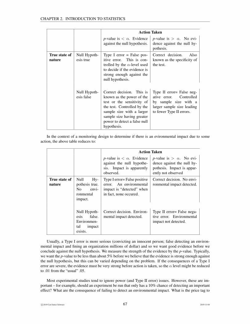
In any experiment, it is never known if one of these errors or a correct decision has been made. TheType I and Type II errors and the two correct decision can be placed into a summary table:
c©2019 Carl James Schwarz 66 2019-11-04
CHAPTER 2. INTRODUCTION TO STATISTICS
Action Takenp-value is < α. Evidenceagainst the null hypothesis.
p-value is > α. No evi-dence against the null hy-pothesis.
True state ofnature
Null Hypoth-esis true
Type I error = False pos-itive error. This is con-trolled by the α-level usedto decide if the evidence isstrong enough against thenull hypothesis.
Correct decision. Alsoknown as the specificity ofthe test.
Null Hypoth-esis false
Correct decision. This isknown as the power of thetest or the sensitivity ofthe test. Controlled by thesample size with a largersample size having greaterpower to detect a false nullhypothesis.
Type II error= False neg-ative error. Controlledby sample size with alarger sample size leadingto fewer Type II errors.
In the context of a monitoring design to determine if there is an evironmental impact due to someaction, the above table reduces to:
Action Takenp-value is < α. Evidenceagainst the null hypothe-sis. Impact is apparentlyobserved.
p-value is > α. No evi-dence against the null hy-pothesis. Impact is appar-ently not observed
True state ofnature
Null Hy-pothesis true.No envi-ronmentalimpact.
Type I error= False positiveerror. An environmentalimpact is “detected” whenin fact, none occured.
Correct decision. No envi-ronmental impact detected.
Null Hypoth-esis false.Environmen-tal impactexists.
Correct decision. Environ-mental impact detected.
Type II error= False nega-tive error. Environmentalimpact not detected.
Usually, a Type I error is more serious (convicting an innocent person; false detecting an environ-mental impact and fining an organization millions of dollar) and so we want good evidence before weconclude against the null hypothesis. We measure the strength of the evidence by the p-value. Typically,we want the p-value to be less than about 5% before we believe that the evidence is strong enough againstthe null hypothesis, but this can be varied depending on the problem. If the consequences of a Type Ierror are severe, the evidence must be very strong before action is taken, so the α level might be reducedto .01 from the “usual” .05.
Most experimental studies tend to ignore power (and Type II error) issues. However, these are im-portant – for example, should an experiment be run that only has a 10% chance of detecting an importanteffect? What are the consequence of failing to detect an environmental impact. What is the price tag to
c©2019 Carl James Schwarz 67 2019-11-04
CHAPTER 2. INTRODUCTION TO STATISTICS
letting a species go extinct without detecting it? We will explore issues of power and sample size in laterchapters.
What is a Type III error? This is more whimsical, as it refers to a correct answer to the wrongquestion! Too often, researchers get caught up in their particular research project and spent much timeand energy in obtaining an answer, but the answer is not relevant to the question of interest.
2.4.5 Some practical advice
• The p-value does NOT measure the probability that the null hypothesis is true. It measures theprobability of observing the sample data assuming the null hypothesis were true. You cannotattach a probability statement to the null hypothesis in the same way you can’t be 90% pregnant!The hypothesis is either true or false – there is no randomness attached to a hypothesis. Therandomness is attached to the data.
• A rough rule of thumb is there is sufficient evidence against the hypothesis if the observed teststatistic is more than 2 se away from the hypothesized value.
• The p-value is also known as the observed significance level. In the past, you choose a prespec-ified significance level (known as the α level) and if the p-value is less than α, you concludedagainst the null hypothesis. For example, α is often set at 0.05 (denoted α =0.05). If the p-valueis < α = 0.05, then you concluded tat the evidence was strong aganst the null hypothesis; other-wise you the evidence was not strong enought against the null hypothesis. Scientific papers oftenreported results using a series of asterisks, e.g. “*” meant that a result was statistically significantat α = .05; “**” meant that a result was statistically significant at α = .01; “***” meant thata result was statistically significant at α = .001. This practice reflects a time when it was quiteimpossible to compute the exact p-values, and only tables were available. In this modern era, thereis no excuse for failing to report the exact p-value. All scientific papers should report the actualp-value for a test so that the reader can use their own personal significance level.
• Some ‘traditional’ and recommended nomenclature for the results of hypothesis testing:
p-value Traditional Recommended
p-value< 0.05
Reject the null hypothesis There is strong evidenceagainst the null hypothesis.
.05 <p-value< .15
Barely fail to reject the nullhypothsis
Evidence is equivocol andwe need more data.
p-value> .15
Fail to reject the null hy-pothesis.
There is no evidenceagainst the null hypothesis.
However, the point at which we conclude that there is sufficient evidence against the null hypoth-esis (the α level which was .05 above) depends upon the situation at hand and the consequencesof wrong decisions (see later in this chapter)..
• It is not good form to state things like:
– accept the null hypothesis;
– accept the alternate hypothesis;
– the null hypothesis is true;
– the null hypothesis is false.
The reason is that you haven’t ‘proved’ the truthfulness or falseness of the hypothesis; ratheryou have not or have sufficient evidence that contradict it. It is the same reasons that jury trialsreturn verdicts of ‘guilty’ (evidence against the hypothesis of innocence) or ‘not guilty’ (insufficentevidence against the hypothesis of innocence). A jury trial does NOT return an ‘innocent’ verdict.
c©2019 Carl James Schwarz 68 2019-11-04
CHAPTER 2. INTRODUCTION TO STATISTICS
• If there is evidence against the null hypothesis, a natural question to ask is ‘well, what value ofthe parameter are plausible given this data’? This is exactly what a confidence interval tells you.Consequently, I usually prefer to find confidence intervals, rather than doing formal hypothesistesting.
• Carrying out a statistical test of a hypothesis is straightforward with many computer packages.However, using tests wisely is not so simple. Hypothesis testing demands the RRR. Any surveyor experiment that doesn’t follow the three basic principles of statistics (randomization, replica-tion, and blocking) is basically useless. In particular, non randomized surveys or experimentsCANNOT be used in hypothesis testing or inference. Be careful that ‘random’ is not confusedwith ‘haphazard’. Computer packages do not know how you collected data. It is your responsibil-ity to ensure that your brain in engaged before putting the package in gear. Each test is valid onlyin circumstances where the method of data collection adheres to the assumptions of the test. Somehesitation about the use of significance tests is a sign of statistical maturity.
• Beware of outliers or other problems with the data. Be prepared to spend a fair amount of timeexamining the raw data for spurious points.
2.4.6 The case against hypothesis testing
In recent years, there has been much debate about the usefulness of hypothesis testing in scientific re-search (see the next section for a selection of articles). There a number of “problems” with the uncriticaluse of hypothesis testing:
• Sharp null hypothesis The value of 98 ppm as a hypothesized value seems rather arbitrary.Why not 97.9 ppm or 98.1 ppm. Do we really think that the population DDT value is exactly98.000000000 ppm? Perhaps it would be more reasonable to ask “How close is the actual meanDDT in the population to 98 ppm?”
• Choice of α The choice of α-level (i.e. 0.05 significance level) is also arbitrary. The value of αshould reflect the costs of Type I errors, i.e. the costs of false positive results. In a murder trial,the cost of sending an innocent person to the electric chair is very large - we require a very largeburden of proof, i.e. the p-value must be very small. On the other hand, the cost of an innocentperson paying for a wrongfully issued parking ticket is not very large; a lesser burden of proof isrequired, i.e. a higher p-value can be used to conclude that the evidence is strong enough againstthe hypothesis.
A similar analysis should be made for any hypothesis testing case, but rarely is done.
The tradeoffs between Type I and II errors, power, and sample size are rarely discussed in thiscontext.
• Sharp decision rules Traditional hypothesis testing says that if the p-value is less than α, youshould conclude that there is sufficient evidence against the null hypothesis and if the p-value isgreater than α there is not enough evidence against the null hypothesis. Suppose that α is set at.05. Should different decisions be made if the p-value is 0.0499 or 0.0501? It seems unlikely thatextremely minor differences in the p-value should lead to such dramatic differences in conclusions.
• Obvious tests In many cases, hypothesis testing is used when the evidence is obvious. For exam-ple, why would you even bother testing if the population mean is 50 ppm? The data clearly showsthat it is not.
• Interpreting p-values P-values are prone to mis-interpretation as they measure the plausibility ofthe data assuming the null hypothesis is true, not the probability that the hypothesis is true. Thereis also the confusion between selecting the appropriate p-value for one- and two-sided tests.
c©2019 Carl James Schwarz 69 2019-11-04
CHAPTER 2. INTRODUCTION TO STATISTICS
Refer to the Ministry of Forest’s publication Pamphlet 30 on interpreting the p-value available athttp://www.stat.sfu.ca/~cschwarz/Stat-650/MOF/index.html.
• Effect of sample size P-values are highly affected by sample size. With sufficiently large samplesizes every effect is statistically significant but may be of no biological interest.
• Practical vs. statistical significance. Just because you find evidence against the null hypothesis(e.g. p-value < .05) does not imply that the effect is very large. For example, if you were to test ifa coin were fair and were able to toss it 1,000,000 times, you would find strong evidence againstthe null hypothesis of fairness if the observed proportion of heads was 50.001%. But for all intentsand purposes, the coin is fair enough for real use. Statistical significance is not the same aspractical significance. Other examples of this trap, are the numerous studies that show cancerouseffects of certain foods. Unfortunately, the estimated increase in risk from these studies is oftenless than 1/100 of 1%!
The remedy for confusing statistical and practical significance is to ask for a confidence intervalfor the actual parameter of interest. This will often tell you the size of the purported effect.
• Failing to detect a difference vs. no effect. Just because an experiment fails to find evidenceagainst the null hypothesis (e.g. p-value > .05) does not mean that there is no effect! A Type IIerror - a false negative error - may have been committed. These usually occur when experimentsare too small (i.e., inadequate sample size) to detect effects of interest.
The remedy for this is to ask for the power of the test to detect the effect of practical interest, orfailing that, ask for the confidence interval for the parameter. Typically power will be low, or theconfidence interval will be so wide as to be useless.
• Multiple testing. In some experiments, hundreds of statistical tests are performed. However,remember that the p-value represents the chance that this data could have occurred given that thehypothesis is true. So a p-value of 0.01 implies, that this event could have occurred in about 1%of cases EVEN IF THE NULL IS TRUE. So finding one or two significant results out of hundredsof tests is not surprising!
There are more sophisticated analyses available to control this problem called ‘multiple compari-son techniques’ and are covered in more advanced classes.
On the other hand, a confidence interval for the population parameter gives much more information.The confidence interval shows you how precise the estimate is, and the range of plausible values that areconsistent with the data collected.
For example consider the following illustration:
c©2019 Carl James Schwarz 70 2019-11-04
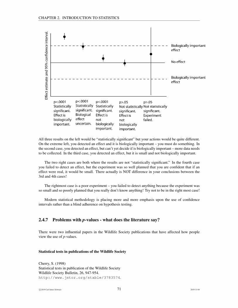
CHAPTER 2. INTRODUCTION TO STATISTICS
All three results on the left would be “statistically significant” but your actions would be quite different.On the extreme left, you detected an effect and it is biologically important – you must do something. Inthe second case, you detected an effect, but can’t yet decide if is biologically important – more data needsto be collected. In the third case, you detected an effect, but it is small and not biologically important.
The two right cases are both where the results are not “statistically significant.” In the fourth caseyou failed to detect an effect, but the experiment was so well planned that you are confident that if aneffect were real, it would be small. There actually is NOT difference in your conclusions between the3rd and 4th cases!
The rightmost case is a poor experiment – you failed to detect anything because the experiment wasso small and so poorly planned that you really don’t know anything! Try not to be in the right most case!
Modern statistical methodology is placing more and more emphasis upon the use of confidenceintervals rather than a blind adherence on hypothesis testing.
2.4.7 Problems with p-values - what does the literature say?
There were two influential papers in the Wildlife Society publications that have affected how peopleview the use of p-values.
Statistical tests in publications of the Wildlife Society
Cherry, S. (1998)Statistical tests in publication of the Wildlife SocietyWildlife Society Bulletin, 26, 947-954.http://www.jstor.org/stable/3783574.
c©2019 Carl James Schwarz 71 2019-11-04
CHAPTER 2. INTRODUCTION TO STATISTICS
The 1995 issue of the Journal of Wildlife Management has > 2400 p-values. I believe thatis too many. In this article, I will argue that authors who publish in the Journal and in heWildlife Society Bulletin are over using and misunderstanding hypothesis tests. They areconducting too many unnecessary tests, and they are making common mistakes in carryingout and interpreting the results of the tests they conduct. A major cause of the overuseof testing in the Journal and the Bulletin seems to be the mistaken belief that testing isnecessary in order for a study to be valid or scientific.
• What are the problems in the analysis of habitat availability.
• What additional information do confidence intervals provide that significance levels do not pro-vide?
• When is the assumption of normality critical, in testing if the means of two population are equal?
• What does Cherry recommend in lieu of hypothesis testing?
The Insignificance of Statistical Significance Testing
Johnson, D. H. (1999)The Insignificance of Statistical Significance TestingJournal of Wildlife Management, 63, 763-772.http://dx.doi.org/10.2307/3802789 or online athttp://www.npwrc.usgs.gov/resource/methods/statsig/index.htm
Despite their wide use in scientific journals such as The Journal of Wildlife Management,statistical hypothesis tests add very little value to the products of research. Indeed, theyfrequently confuse the interpretation of data. This paper describes how statistical hypoth-esis tests are often viewed, and then contrasts that interpretation with the correct one. Hediscusses the arbitrariness of p-values, conclusions that the null hypothesis is true, poweranalysis, and distinctions between statistical and biological significance. Statistical hypoth-esis testing, in which the null hypothesis about the properties of a population is almostalways known a priori to be false, is contrasted with scientific hypothesis testing, whichexamines a credible null hypothesis about phenomena in nature. More meaningful alter-natives are briefly outlined, including estimation and confidence intervals for determiningthe importance of factors, decision theory for guiding actions in the face of uncertainty, andBayesian approaches to hypothesis testing and other statistical practices.
This is a very nice, readable paper, that discusses some of the problems with hypothesis testing. Asin the Cherry paper above, Johnson recommends that confidence intervals be used in place of hypothesistesting.
So why are confidence intervals not used as often as they should? Johnson give several reasons
• hypothesis testing has become a tradition;
• the advantages of confidence intervals are not recognized;
• there is some ignorance of the procedures available;
• major statistical packages do not include many confidence interval estimates;
c©2019 Carl James Schwarz 72 2019-11-04
CHAPTER 2. INTRODUCTION TO STATISTICS
• sizes of parameter estimates are often disappointingly small even though they may be very signif-icantly different from zero;
• the wide confidence intervals that often result from a study are embarrassing;
• some hypothesis tests (e.g., chi square contingency table) have no uniquely defined parameterassociated with them; and
• recommendations to use confidence intervals often are accompanied by recommendations to aban-don statistical tests altogether, which is unwelcome advice.
These reasons are not valid excuses for avoiding confidence intervals in lieu of hypothesis tests in situa-tions for which parameter estimation is the objective.
Followups
In
Robinson, D. H. and Wainer, H. W. (2002).On the past and future of null hypothesis significance testing.Journal of Wildlife Management 66, 263-271.http://dx.doi.org/10.2307/3803158.
the authors argue that there is some benefit to p-values in wildlife management, but then
Johnson, D. H. (2002).The role of hypothesis testing in wildlife science.Journal of Wildlife Management 66, 272-276.http://dx.doi.org/10.2307/3803159.
counters many of these arguments. Both papers are very easy to read and are highly recommended.
2.5 Meta-data
Meta-data are data about data, i.e. how has it been collected, what are the units, what do the codes usedin the dataset represent, etc. It is good practice to store the meta-data as close as possible to the rawdata. For example, some computer packages (e.g. JMP) allow the user to store information about eachvariable and about the data table.
In some cases, data can be classified into broad classifications called scale or roles.
2.5.1 Scales of measurement
Data comes in various sizes and shapes and it is important to know about these so that the proper analysiscan be used on the data.
c©2019 Carl James Schwarz 73 2019-11-04
CHAPTER 2. INTRODUCTION TO STATISTICS
Some computer packages (e.g. JMP) use the scales of measurement to determine appropriate anal-yses of the data. For example, as you will see later in the course, if the response variable (Y ) has aninterval scale and the explanatory variable (X) has a‘ nominal scale, then an ANOVA-type analysis com-paring means is performed. If both the Y and X variables have a nominal scale, then a χ2-type analysison comparing proportions is performed.
There are usually 4 scales of measurement that must be considered:
1. Nominal Data
• The data are simply classifications.
• The data have no ordering.
• The data values are arbitrary labels.
• An example of nominal data is sex using codes m and f , or (not recommended) codes 0 and1. Note that just because a numeric code is used for sex, the variable is still nominally scaled.The practice of using numeric codes for nominal data is discouraged (see below).
2. Ordinal Data
• The data can be ordered but differences between values cannot be quantified.
• Some examples of ordinal data are:
– Ranking political parties on left to right spectrum using labels 0, 1, or 2.– Using a Likert scale to rank you degree of happiness on a scale of 1 to 5.– Giving a restaurant ratings as terrific, good, or poor.– Ranking the size of animals as small, medium, large or coded as 1, 2, 3. Again numeric
codes for ordinal data are discouraged (see below).
3. Interval Data
• The data can be ordered, have a constant scale, but have no natural zero.
• This implies that differences between data values are meaningful, but ratios are not.
• There are really only two common interval scaled variables, e.g., temperature (◦C, ◦F), dates.For example, 30◦ C − 20◦ C = 20◦ C − 10◦ C, but 20◦ C/10◦ C is not twice as hot!
4. Ratio Data
• Data can be ordered, have a constant scale, and have a natural zero.
• Examples of ratio data are height, weight, age, length, etc.
Categorical data is another term often applied to nominal or ordinal data.
Some packages (e.g. JMP) make no distinction between Interval or Ratio data, labelling both of themas ‘continuous’. However, this is, technically, not quite correct.
Only certain operations can be performed on certain scales of measurement. The following listsummarizes which operations are legitimate for each scale. Note that you can always apply operationsfrom a ‘lesser scale’ to any particular data, e.g. you may apply nominal, ordinal, or interval operationsto an interval scaled datum.
• Nominal Scale. You are only allowed to examine if a nominal scale datum is equal to someparticular value or to count the number of occurrences of each value. For example, gender is a
c©2019 Carl James Schwarz 74 2019-11-04
CHAPTER 2. INTRODUCTION TO STATISTICS
nominal scale variable. You can examine if the gender of a person is F or count the number ofmales in a sample. Talking the average of nominally scaled data is not sensible (e.g. the averagesex is not sensible).
In order to avoid problems with computer packages trying to take averages of nominal data, it isrecommended that alphanumerical codes be used for nominally scaled data, e.g. use M and F forsex rather than 0 or 1. Most packages can accept alphanumeric data without problems.
• Ordinal Scale. You are also allowed to examine if an ordinal scale datum is less than or greaterthan another value. Hence, you can ‘rank’ ordinal data, but you cannot ‘quantify’ differencesbetween two ordinal values. For example, political party is an ordinal datum with the NDP to theleft of the Conservative Party, but you can’t quantify the difference. Another example is preferencescores, e.g. ratings of eating establishments where 10 = good and 1 = poor, but the differencebetween an establishment with a 10 ranking and an 8 ranking can’t be quantified.
Technically speaking, averages are not really allowed for ordinal data, e.g. taking the averageof small, medium and large as data values doesn’t make sense. Again alphanumeric codes arerecommended for ordinal data. Some case should be taken with ordinal data and alphanumericcodes as many packages sort values alphabetically and so the ordering of large, medium , smallmay not correspond to the ordering desired. JMP allows the user to specify the ordering of valuesin the Column Information of each variable. A simple trick to get around this problem, is to usealphanumeric codes such as 1.small, 2.medium, 3.large as the data values as an alphabetic sortthen keeps the values in proper order.
• Interval Scale. You are also allowed to quantify the difference between two interval scale valuesbut there is no natural zero. For example, temperature scales are interval data with 25◦ C warmerthan 20◦C and a 5◦ C difference has some physical meaning. Note that 0◦ C is arbitrary, so that itdoes not make sense to say that 20◦ C is twice as hot as 10◦ C.
Values for interval scaled variables are recorded using numbers so that averages can be taken.
• Ratio Scale. You are also allowed to take ratios among ratio scaled variables. Physical measure-ments of height, weight, length are typically ratio variables. It is now meaningful to say that 10 mis twice as long as 5 m. This ratio hold true regardless of which scale the object is being measuredin (e.g. meters or yards). This is because there is a natural zero.
Values for ratio scaled variables are recorded as numbers so that averages can be taken.
2.5.2 Types of Data
Data can also be classified by its type. This is less important than the scale of measurement, as it usuallydoes not imply a certain type of analysis, but can have subtle effects.
Discrete data Only certain specific values are valid, points between these values are not valid. Forexample, counts of people (only integer values allowed), the grade assigned in a course (F, D, C-,C, C+, . . .).
Continuous data All values in a certain range are valid. For example, height, weight, length, etc. Notethat some packages label interval or ratio data as continuous. This is not always the case.
Continuous but discretized Continuous data cannot be measured to infinite precision. It must be dis-cretized, and consequently is technically discrete. For example, a person’s height may be measuredto the nearest cm. This can cause problems if the level of discretization is too coarse. For example,what would happen if a person’s height was measured to the nearest meter.
As a rule of thumb, if the discretization is less than 5% of the typical value, then a discretizedcontinuous variable can be treated as continuous without problems.
c©2019 Carl James Schwarz 75 2019-11-04
CHAPTER 2. INTRODUCTION TO STATISTICS
2.5.3 Roles of data
Some computer packages (e.g. JMP) also make distinctions about the role of a variable.
Label A variable whose value serves as an identification of each observation - usually for plotting.
Frequency A variable whose value indicates how many occurrences of this observation occur. Forexample, rather than having 100 lines in a data set to represent 100 females, you could have oneline with a count of 100 in the Frequency variable.
Weight This is rarely used. It indicates the weight that this observation is to have in the analysis. Usuallyused in advanced analyses.
X Identifies a variables as a ‘predictor’ variable. [Note that the use of the term ‘independent’ variable issomewhat old fashioned and is falling out of favour.] This will be more useful when actual dataanalysis is started.
Y Identifies a variable as a ‘response’ variable. [Note tht the use of the term ‘dependent’ variable issomewhat old fashione and is falling out of favour.] This will be more useful when actual dataanalysis is started.
2.6 Bias, Precision, Accuracy
The concepts of Bias, Precision and Accuracy are often used interchangeably in non-technical writingand speaking. However these have very specific statistical meanings and it important that these becarefully differentiated.
The first important point about these terms is that they CANNOT be applied in the context of asingle estimate from a single set of data. Rather, they are measurements of the performance of anestimator over repeated samples from the same population. Recall, that a fundamental idea of statisticsis that repeated samples from the same population will give different estimates, i.e. estimates will varyas different samples are selected.9
Bias is the difference between average value of the estimator over repeated sampling from the pop-ulation and the population parameter value. If the estimates from repeated sampling vary above andbelow the population parameter value so that the average over all possible samples equals the populationparameter value, we say that the estimator is unbiased.
There are two types of bias - systemic and statistical. Systemic Bias is caused by problems in theapparatus or the measuring device. For example, if a scale systematically gave readings that were 10 gtoo small, this would be a systemic bias. Or is snorkelers in stream survey consistently only see 50% ofthe available fish, this would also be an example of systemic bias. Statistical bias is related to the choiceof sampling design and estimator. For example, the usual sample statistics in an simple random samplegive unbiased estimates of means, totals, variances, but not for standard deviations. The ratio estimatorof survey sampling (refer to later chapters) is also biased.
It is not possible to detect systemic biases using the data ta hand. The researcher must examinethe experimental apparatus and design very carefully. For example, if repeated surveys were made bysnorkeling over sections of streams, estimates may be very reproducible (i.e. very precise) but could beconsistently WRONG, i.e. divers only see about 60% of the fish (i.e. biased). Systemic Bias is controlled
9The standard error of a estimator measures this variation over repeated samples from the same population.
c©2019 Carl James Schwarz 76 2019-11-04
CHAPTER 2. INTRODUCTION TO STATISTICS
by careful testing of the experimental apparatus etc. In some cases, it is possible to calibrate the methodusing "known" populations, – e.g. mixing a solution of a known concentration and then having yourapparatus estimate the concentration.
Statistical biases can be derived from statistical theory. For example, statistical theory can tell youthat the sample mean of a simple random sample is unbiased for the population mean; that the sampleVARIANCE is unbiased for the population variance; but that the sample standard deviation is a biasedestimator for the population standard deviation. [Even though the sample variance is unbiased, thesample standard deviation is a NON-LINEAR function of the variance (i.e. square-rooted) and non-linear functions don’t preserve unbiasedness.] The ratio estimator is also biased for the population ratio.In many cases, the statistical bias can be shown to essentially disappear with reasonably large samplesizes.
Precision of an estimator refers to how variable the repeated estimates will be over repeated samplingfrom the same population. Again recall that every different sample from the same population will leadto a different estimate. If these estimates have very little variation over repeated sample, we say that theestimate is precise. The standard error (SE) of the estimator measures the variation of the estimator overrepeated sampling from the same population.
The precision of an estimator is controlled by the sample size. In general, a larger sample size leadsto more precise estimates than a smaller sample size.
The precision of an estimator is also determined by statistical theory. For example, the precision(standard error) of a sample mean selected using a simple random sample from a large population isfound using mathematics to be equal to pop std dev√
n. A common error is to use this latter formula for all
estimators that look like a mean – however the formula for the standard error of any estimator dependsupon the way the data are collected (i.e. is a simple random sample, a cluster sample, a stratified sampleetc), the estimator of interest (e.g. different formulae are used for standard errors of mean, proportions,total, slopes etc.) and, in some cases, the distribution of the population values (e.g. do elements from thepopulation come from a normal distribution, or a Weibull distribution, etc.).
Finally, accuracy is a combination of precision and bias. It measures the “average distance” of theestimator from the population parameter. Technically, one measure of the accuracy of an estimator isthe Root Mean Square Error (RMSE) and is computed as
√(Bias)2 + (SE)2. A precise, unbiased
estimator will be accurate, but not all accurate estimators will be unbiased.
The relationship between bias, precision, and accuracy can be view graphically as shown below. Let* represent the population parameter value (say the population mean), and periods (.) represent values
c©2019 Carl James Schwarz 77 2019-11-04
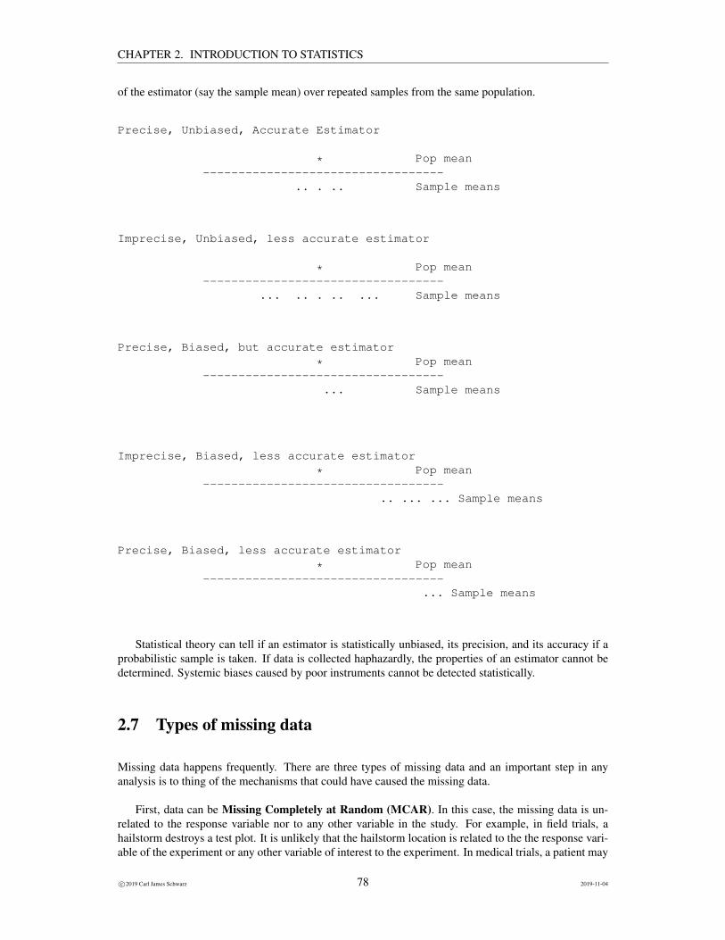
CHAPTER 2. INTRODUCTION TO STATISTICS
of the estimator (say the sample mean) over repeated samples from the same population.
Precise, Unbiased, Accurate Estimator
* Pop mean----------------------------------
.. . .. Sample means
Imprecise, Unbiased, less accurate estimator
* Pop mean----------------------------------
... .. . .. ... Sample means
Precise, Biased, but accurate estimator
* Pop mean----------------------------------
... Sample means
Imprecise, Biased, less accurate estimator
* Pop mean----------------------------------
.. ... ... Sample means
Precise, Biased, less accurate estimator
* Pop mean----------------------------------
... Sample means
Statistical theory can tell if an estimator is statistically unbiased, its precision, and its accuracy if aprobabilistic sample is taken. If data is collected haphazardly, the properties of an estimator cannot bedetermined. Systemic biases caused by poor instruments cannot be detected statistically.
2.7 Types of missing data
Missing data happens frequently. There are three types of missing data and an important step in anyanalysis is to thing of the mechanisms that could have caused the missing data.
First, data can be Missing Completely at Random (MCAR). In this case, the missing data is un-related to the response variable nor to any other variable in the study. For example, in field trials, ahailstorm destroys a test plot. It is unlikely that the hailstorm location is related to the the response vari-able of the experiment or any other variable of interest to the experiment. In medical trials, a patient may
c©2019 Carl James Schwarz 78 2019-11-04
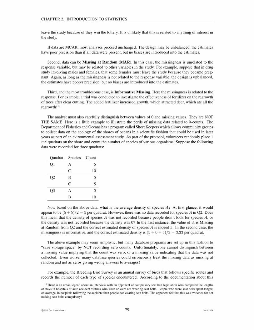
CHAPTER 2. INTRODUCTION TO STATISTICS
leave the study because of they win the lottery. It is unlikely that this is related to anything of interest inthe study.
If data are MCAR, most analyses proceed unchanged. The design may be unbalanced, the estimateshave poor precision than if all data were present, but no biases are introduced into the estimates.
Second, data can be Missing at Random (MAR). In this case, the missingness is unrelated to theresponse variable, but may be related to other variables in the study. For example, suppose that in drugstudy involving males and females, that some females must leave the study because they became preg-nant. Again, as long as the missingness is not related to the response variable, the design is unbalanced,the estimates have poorer precision, but no biases are introduced into the estimates.
Third, and the most troublesome case, is Informative Missing. Here the missingness is related to theresponse. For example, a trial was conducted to investigate the effectiveness of fertilizer on the regrowthof trees after clear cutting. The added fertilizer increased growth, which attracted deer, which ate all theregrowth!10
The analyst must also carefully distinguish between values of 0 and missing values. They are NOTTHE SAME! Here is a little example to illustrate the perils of missing data related to 0-counts. TheDepartment of Fisheries and Oceans has a program called ShoreKeepers which allows community groupsto collect data on the ecology of the shores of oceans in a scientific fashion that could be used in lateryears as part of an evironmental assessment study. As part of the protocol, volunteers randomly place 1m2 quadrats on the shore and count the number of species of various organisms. Suppose the followingdata were recorded for three quadrats:
Quadrat Species Count
Q1 A 5
C 10
Q2 B 5
C 5
Q3 A 5
B 10
Now based on the above data, what is the average density of species A? At first glance, it wouldappear to be (5 + 5)/2 = 5 per quadrat. However, there was no data recorded for species A in Q2. Doesthis mean that the density of species A was not recorded because people didn’t look for species A, orthe density was not recorded because the density was 0? In the first instance, the value of A is Missingat Random from Q2 and the correct estimated density of species A is indeed 5. In the second case, themissingness is informative, and the correct estimated density is (5 + 0 + 5)/3 = 3.33 per quadrat.
The above example may seem simplistic, but many database programs are set up in this fashion to“save storage space” by NOT recording zero counts. Unfortunately, one cannot distinguish betweena missing value implying that the count was zero, or a missing value indicating that the data was notcollected. Even worse, many database queries could erroneously treat the missing data as missing atrandom and not as zeros giving wrong answers to averages!
For example, the Breeding Bird Survey is an annual survey of birds that follows specific routes andrecords the number of each type of species encountered. According to the documentation about this
10There is an urban legend about an interview with an opponent of compulsory seat belt legislation who compared the lengthsof stays in hospitals of auto accident victims who were or were not wearing seat belts. People who wore seat belts spent longer,on average, in hospitals following the accident than people not wearing seat belts. The opponent felt that this was evidence for notmaking seat belts compulsory!
c©2019 Carl James Schwarz 79 2019-11-04
CHAPTER 2. INTRODUCTION TO STATISTICS
survey11 only the non-zero counts are stored in the database and some additional information such as thenumber of actual routes run is required to impute the missing zeroes:
“Since only non-zero counts are included in the database, the complete list of years a routeis run allows the times in which the species wasn’t seen to be identified and included in thedata analysis.”
If this extra step was not done, then you would be in the exact problem above on quadrat sampling.
The moral of the story is that 0 is a valid value and should be recorded as such! Computer storagecosts are declining so quickly, that the “savings” by not recording 0’s soon vanish when people can’t ordon’t remember to adjust for the unrecorded 0 values.
If your experiment or survey has informative missing values, you could have a serious problem inthe analysis and expert help should be consulted.
2.8 Transformations
2.8.1 Introduction
Many of the procedures in this course have an underlying assumption that the data from each group isnormally distributed with a common variance. In some cases this is patently false, e.g. the data arehighly skewed with variances that change, often with the mean.
The most common method to fix this problem is a transformation of the data and the most commontransformation in ecology is the logarithmic transform, i.e. analyze the log(Y ) rather than Y . Othertransformations are possible - these will not be discussed in this course, but the material below appliesequally well to these other transformations.
If you are unsure of the proper transformation, there are a number of methods than can assist includ-ing a Box-Cox Transform and an applicaiton of Taylor’s Power Law. These are beyond the scope of thiscourse.
The logarithmic transform is often used when the data are positive and exhibit a pronounced longright tail. For example, the following are plots of (made-up) data before and after a logarithmic transfor-mation:
11http://www.cws-scf.ec.gc.ca/nwrc-cnrf/migb/stat_met_e.cfm
c©2019 Carl James Schwarz 80 2019-11-04
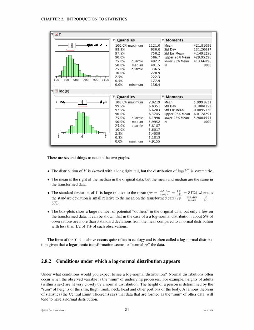
CHAPTER 2. INTRODUCTION TO STATISTICS
There are several things to note in the two graphs.
• The distribution of Y is skewed with a long right tail, but the distribution of log(Y ) is symmetric.
• The mean is the right of the median in the original data, but the mean and median are the same inthe transformed data.
• The standard deviation of Y is large relative to the mean (cv = std devmean = 131
421 = 31%) where asthe standard deviation is small relative to the mean on the transformed data (cv = std dev
mean = .36.0 =
5%).
• The box-plots show a large number of potential “outliers” in the original data, but only a few onthe transformed data. It can be shown that in the case of a a log-normal distribution, about 5% ofobservations are more than 3 standard deviations from the mean compared to a normal distributionwith less than 1/2 of 1% of such observations.
The form of the Y data above occurs quite often in ecology and is often called a log-normal distribu-tion given that a logarithmic transformation seems to “normalize” the data.
2.8.2 Conditions under which a log-normal distribution appears
Under what conditions would you expect to see a log-normal distribution? Normal distributions oftenoccur when the observed variable is the “sum” of underlying processes. For example, heights of adults(within a sex) are fit very closely by a normal distribution. The height of a person is determined by the“sum” of heights of the shin, thigh, trunk, neck, head and other portions of the body. A famous theoremof statistics (the Central Limit Theorem) says that data that are formed as the “sum” of other data, willtend to have a normal distribution.
c©2019 Carl James Schwarz 81 2019-11-04
CHAPTER 2. INTRODUCTION TO STATISTICS
In some cases, the underlying process act multiplicatively. For example, the distribution of householdincome is often a log-normal distribution. You can imagine that factor such as level of education, mo-tivation, parental support act to “multiply” income rather than simply adding a fixed amount of money.Similarly, data on animal abundance often has a log-normal distribution because factors such as survivalact multiplicatively on the populations.
2.8.3 ln() vs. log()
There is often much confusion about the form of the logarithmic transformation. For example, manycalculators and statistical packages differential between the common logarithm (base 10, or log) and thenatural logarithm (base e or ln). Even worse, is that many packages actually use log to refer to naturallogarithms and log 10 to refer to common logarithms. IT DOESN’T MATTER which transformation isused as long as the proper back-transformation is applied. When you compare the actual values afterthese transformations, you will see that ln(Y ) = 2.3 log10(Y ), i.e. the log-transformed values differ bya fixed multiplicative constant. When the anti-logs are applied this constant will “disappear”.
In accordance with common convention in statistics and mathematics, the use of log(Y ) will refer tothe natural or ln(Y ) transformation.
2.8.4 Mean vs. Geometric Mean
The simple mean of Y is called the arithmetic mean (or simply) the mean and is computed in the usualfashion.
The anti-log of the mean of the log(Y ) values is called the geometric mean. The geometric mean ofa set of data is ALWAYS less than the mean of the original data. In the special case of log-normal data,the geometric mean will be close to the MEDIAN of the original data.
For example, look that the data above. The mean of Y is 421. The mean of log(Y ) is 5.999 andexp(5.999) = 403 which is close to the median of the original data.
This implies that when reporting results, you will need to be a little careful about how the back-transformed values are interpreted.
It is possible to go from the mean on the log-scale to the mean on the anti-log scale and vice-versa.For log-normal data,12 it turns out that
Y antilog ≈ exp(Y log +s2log
2)
and
Y log ≈ log(Y antilog)−s2antilog
2Y2
antilog
In this case:
Y antilog ≈ exp(5.999 +(.3)2
2) = 422.
and
Y log ≈ log(421.81)− 131.22
2× 421.82= 5.996
12Other transformation will have a different formula
c©2019 Carl James Schwarz 82 2019-11-04
CHAPTER 2. INTRODUCTION TO STATISTICS
Unfortunately, the formula for the standard deviations is not as straight forward. There is somewhatcomplicated formula available in many reference books, but a close approximation is that:
sanitlog ≈ slog × exp(Y log)
andslog ≈
santilog
Y antilog
For the data above we see that:
santilog ≈ .3× exp(5.999) = 121
andslog ≈
131.21
421.81=, 311
which is close, but not exactly on the money.
2.8.5 Back-transforming estimates, standard errors, and ci
Once inference is made on the transformed scale, it is often nice to back-transform and report results onthe original scale.
For example, a study of turbidity (measured in NTU) on a stream in BC gave the following resultson the log-scale:
Statistics value
Mean on log scale 5.86
Std Dev on log scale .96
SE on log scale 0.27
upper 95% ci Mean 6.4
lower 95% ci Mean 5.3
How should these be reported on the original NTU scale?
Mean on log-scale back to MEDIAN on anti-log scale
The simplest back-transform goes from the mean on the log-scale to the MEDIAN on the anti-log scale.The distribution is often symmetric on the log-scale so the mean, median, and mode on the log-scaleall co-incide. However, when you take anti-logs, the upper tail gets larger much faster than the lowertail and the anti-log transform re-introduces skewness into the back-transformed data. Hence, the centerpoint on the log-scale gets back-transformed to the median on the anti-logscale.
The estimated MEDIAN (or GEOMETRIC MEAN) on the original scale is found by the back trans-form of the mean on the log-scale, i.e.
mediananti-log = exp(meanlog−scale)
estimated median = exp(5.86) = 350 NTU.
The 95% confidence interval for the MEDIAN is found by doing a simple back-transformation onthe 95% confidence interval for the mean on the log-scale, i.e. from exp(5.3) = 196 to exp(6.4) =
c©2019 Carl James Schwarz 83 2019-11-04
CHAPTER 2. INTRODUCTION TO STATISTICS
632 NTUs. Note that the confidence interval on the back-transformed scale is no longer symmetricabout the estimate.
There is no direct back-transformation of the standard error from the log-scale to the original scale,but an approximate standard error on the back-transformed scale is found as seantilog = selog×exp(5.86) =95 NTUs.
If the MEAN on the anti-log scale is needed, recall from the previous section that
Meanantilog ≈ exp(Meanlog +std dev2
log
2)
Meanantilog ≈ exp(Meanlog)× exp(std dev2
log
2)
Meanantilog ≈ Median× exp(std dev2
log
2)
Meanantilog ≈ Median× exp(.962
2) = Median× 1.58.
Hence multiply the median, standard error of the median, and limits of the 95% confidence interval allby 1.58.
2.8.6 Back-transforms of differences on the log-scale
Some care must be taken when back-transforming differences on the log-scale. The general rule ofthumb is that a difference on the log-sacle corresponds to a log(ratio) on the original scale. Hence aback-transform of a difference on the log-scale corresponds to a ratio on the original scale.13
For example, here are the results from a study to compare turbidity before and after remediation wascompleted on a stream in BC.
Statistics value on log-scale
Difference −0.8303
Std Err Dif 0.3695
Upper CL Dif −0.0676
Lower CL Dif −1.5929
p-value 0.0341
A difference of −.83 units on the log-scale corresponds to a ratio of exp(−.83) = .44 in the NTUon the original scale. In otherwords, the median NTU after remediation was .44 times that of the medianNTU before mediation. Of the median NTU before remediation was exp(.83) = 2.29 times that of themedian NTU after remediation. Note that 2.29 = 1/0.44.
The 95% confidence intervals are back-tranformed in a similar fashion. In this case the 95% confi-dence interval on the RATIO of median NTUs lies between exp(−1.59) = .20 to exp(−.067) = .93,i.e. the median NTU after remediation was between .20 and .95 of the median NTU before remediation.
If necessary you could also back-transform the standard error to get a standard error for the ratio onthe original scale, but this is rarely done.
13Recall that log(YZ) = log(Y )− log(Z)
c©2019 Carl James Schwarz 84 2019-11-04

CHAPTER 2. INTRODUCTION TO STATISTICS
2.8.7 Some additional readings on the log-transform
Here are some additional readings on the use of the log-transform taken from the WWW. The URL ispresented at the bottom of each page.
c©2019 Carl James Schwarz 85 2019-11-04

Stats: Log transformation 2/18/05 10:51
- 1 (7) -
http://www.cmh.edu/stats/model/linear/log.asp
Search
Stats >> Model >> Log transformation
Dear Professor Mean, I have some data that I need help with analysis. One suggestion is that I use a logtransformation. Why would I want to do this? -- Stumped Susan
Dear Stumped
Think of it as employment security for us statisticians.
Short answer
If you want to use a log transformation, you compute the logarithm of each data value andthen analyze the resulting data. You may wish to transform the results back to the originalscale of measurement.
The logarithm function tends to squeeze together the larger values in your data set andstretches out the smaller values. This squeezing and stretching can correct one or more of thefollowing problems with your data:
1. Skewed data2. Outliers3. Unequal variation
Not all data sets will suffer from these problems. Even if they do, the log transformation is notguaranteed to solve these problems. Nevertheless, the log transformation works surprisinglywell in many situations.
Furthermore, a log transformation can sometimes simplify your statistical models. Somestatistical models are multiplicative: factors influence your outcome measure throughmultiplication rather than addition. These multiplicative models are easier to work with after alog transformation.
If you are unsure whether to use a log transformation, here are a few things you should lookfor:
1. Is your data bounded below by zero?2. Is your data defined as a ratio?3. Is the largest value in your data more than three times larger than the smallest
value?
86
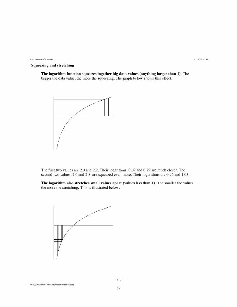
Stats: Log transformation 2/18/05 10:51
- 2 (7) -
http://www.cmh.edu/stats/model/linear/log.asp
Squeezing and stretching
The logarithm function squeezes together big data values (anything larger than 1). Thebigger the data value, the more the squeezing. The graph below shows this effect.
The first two values are 2.0 and 2.2. Their logarithms, 0.69 and 0.79 are much closer. Thesecond two values, 2.6 and 2.8, are squeezed even more. Their logarithms are 0.96 and 1.03.
The logarithm also stretches small values apart (values less than 1). The smaller the valuesthe more the stretching. This is illustrated below.
87

Stats: Log transformation 2/18/05 10:51
- 3 (7) -
http://www.cmh.edu/stats/model/linear/log.asp
The values of 0.4 and 0.45 have logarithms (-0.92 and -0.80) that are further apart. The valuesof 0.20 and 0.25 are stretched even further. Their logarithms are -1.61 and -1.39, respectively.
Skewness
If your data are skewed to the right, a log transformation can sometimes produce a dataset that is closer to symmetric. Recall that in a skewed right distribution, the left tail (thesmaller values) is tightly packed together and the right tail (the larger values) is widely spreadapart.
The logarithm will squeeze the right tail of the distribution and stretch the left tail, whichproduces a greater degree of symmetry.
If the data are symmetric or skewed to the left, a log transformation could actually makethings worse. Also, a log transformation is unlikely to be effective if the data has a narrowrange (if the largest value is not more than three times bigger than the smallest value).
Outliers
If your data has outliers on the high end, a log transformation can sometimes help. Thesqueezing of large values might pull that outlier back in closer to the rest of the data. If yourdata has outliers on the low end, the log transformation might actually make the outlier worse,since it stretches small values.
Unequal variation
Many statistical procedures require that all of your subject groups have comparablevariation. If you data has unequal variation, then the some of your tests and confidenceintervals may be invalid. A log transformation can help with certain types of unequal variation.
A common pattern of unequal variation is when the groups with the large means also tendto have large standard deviations. Consider housing prices in several different neighborhoods.In one part of town, houses might be cheap, and sell for 60 to 80 thousand dollars. In a differentneighborhood, houses might sell for 120 to 180 thousand dollars. And in the snooty part oftown, houses might sell for 400 to 600 thousand dollars. Notice that as the neighborhoods gotmore expensive, the range of prices got wider. This is an example of data where groups withlarge means tend to have large standard deviations.
88
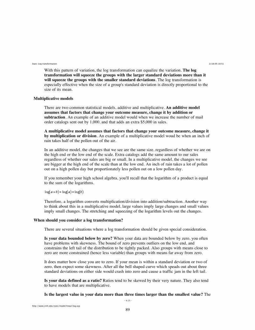
Stats: Log transformation 2/18/05 10:51
- 4 (7) -
http://www.cmh.edu/stats/model/linear/log.asp
With this pattern of variation, the log transformation can equalize the variation. The logtransformation will squeeze the groups with the larger standard deviations more than itwill squeeze the groups with the smaller standard deviations. The log transformation isespecially effective when the size of a group's standard deviation is directly proportional to thesize of its mean.
Multiplicative models
There are two common statistical models, additive and multiplicative. An additive modelassumes that factors that change your outcome measure, change it by addition orsubtraction. An example of an additive model would when we increase the number of mailorder catalogs sent out by 1,000, and that adds an extra $5,000 in sales.
A multiplicative model assumes that factors that change your outcome measure, change itby multiplication or division. An example of a multiplicative model woud be when an inch ofrain takes half of the pollen out of the air.
In an additive model, the changes that we see are the same size, regardless of whether we are onthe high end or the low end of the scale. Extra catalogs add the same amount to our salesregardless of whether our sales are big or small. In a multiplicative model, the changes we seeare bigger at the high end of the scale than at the low end. An inch of rain takes a lot of pollenout on a high pollen day but proportionately less pollen out on a low pollen day.
If you remember your high school algebra, you'll recall that the logarithm of a product is equalto the sum of the logarithms.
Therefore, a logarithm converts multiplication/division into addition/subtraction. Another wayto think about this in a multiplicative model, large values imply large changes and small valuesimply small changes. The stretching and squeezing of the logarithm levels out the changes.
When should you consider a log transformation?
There are several situations where a log transformation should be given special consideration.
Is your data bounded below by zero? When your data are bounded below by zero, you oftenhave problems with skewness. The bound of zero prevents outliers on the low end, andconstrains the left tail of the distribution to be tightly packed. Also groups with means close tozero are more constrained (hence less variable) than groups with means far away from zero.
It does matter how close you are to zero. If your mean is within a standard deviation or two ofzero, then expect some skewness. After all the bell shaped curve which speads out about threestandard deviations on either side would crash into zero and cause a traffic jam in the left tail.
Is your data defined as a ratio? Ratios tend to be skewed by their very nature. They also tendto have models that are multiplicative.
Is the largest value in your data more than three times larger than the smallest value? The
89

Stats: Log transformation 2/18/05 10:51
- 5 (7) -
http://www.cmh.edu/stats/model/linear/log.asp
relative stretching and squeezing of the logarithm only has an impact if your data has a widerange. If the maximum of your data is not at least three times as big as your minimum, then thelogarithm can't squeeze and stretch your data enough to have any useful impact.
Example
The DM/DX ratio is a measure of how rapidly the body metabolizes certain types ofmedication. A patient is given a dose of dextrometorphan (DM), a common cough medication.The patients urine is collected for four hours, and the concentrations of DM and DX (ametabolite of dextrometorphan) are measured. The ratio of DM concentration to DX is ameasure of how well the CYD 2D6 metabolic pathway functions. A ratio less than 0.3 indicatesnormal metabolism; larger ratios indicate slow metabolism.
Genetics can influence CYP 2D6 metabolism. In this set of 206 patients, we have 15 with nofunctional alleles and 191 with one or more functional alleles.
The DM/DX ratio is a good candidate for a log transformation since it is bounded below byzero. It is also obviously a ratio. The standard deviation for this data (0.4) is much larger thanthe mean (0.1).
Finally, the largest value is several orders of magnitude bigger than the smallest value.
Skewness
The boxplots below show the original (untransformed) data for the 15 patients with nofunctional alleles. The graph also shows the log transformed data. Notice that the untransformeddata shows quite a bit of skewness. The lower whisker and the lower half of the box are muchpacked tightly, while the upper whisker and the upper half of the box are spread widely.
The log transformed data, while not perfectly symmetric, does tend to have a better balancebetween the lower half and the upper half of the distribution.
90
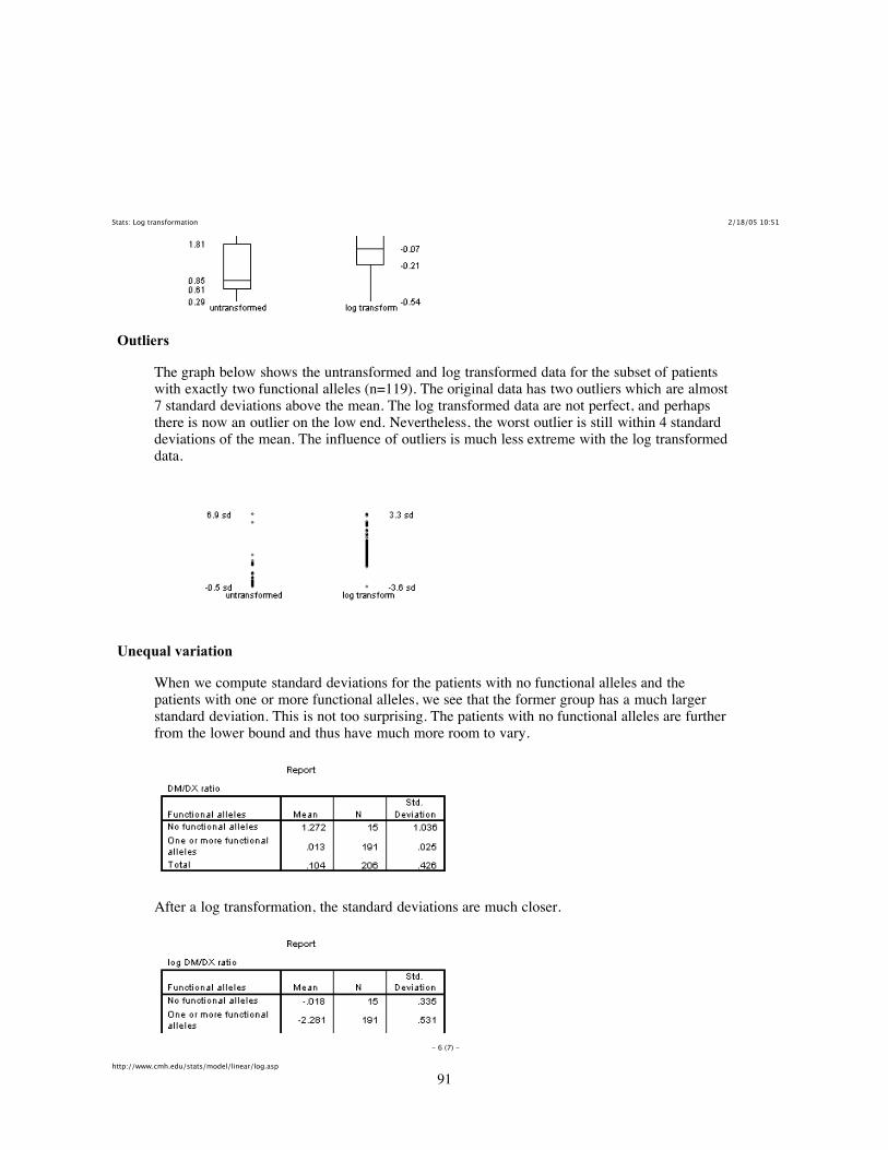
Stats: Log transformation 2/18/05 10:51
- 6 (7) -
http://www.cmh.edu/stats/model/linear/log.asp
Outliers
The graph below shows the untransformed and log transformed data for the subset of patientswith exactly two functional alleles (n=119). The original data has two outliers which are almost7 standard deviations above the mean. The log transformed data are not perfect, and perhapsthere is now an outlier on the low end. Nevertheless, the worst outlier is still within 4 standarddeviations of the mean. The influence of outliers is much less extreme with the log transformeddata.
Unequal variation
When we compute standard deviations for the patients with no functional alleles and thepatients with one or more functional alleles, we see that the former group has a much largerstandard deviation. This is not too surprising. The patients with no functional alleles are furtherfrom the lower bound and thus have much more room to vary.
After a log transformation, the standard deviations are much closer.
91

Stats: Log transformation 2/18/05 10:51
- 7 (7) -
http://www.cmh.edu/stats/model/linear/log.asp
Summary
Stumped Susan wants to understand why she should use a log transformation for her data.Professor Mean explains that a log transformation is often useful for correcting problems withskewed data, outliers, and unequal variation. This works because the log function squeezesthe large values of your data together and stretches the small values apart. The logtransformation is also useful when you believe that factors have a mutliplicative effect. Youshould consider a log transformation when your data are bound below by zero, when you dataare defined as a ratio, and/or when the largest value in your data is at least three times as big asthe smallest value.
Related pages in Stats
Stats: Geometric mean
Further reading
The log transformation is special. Keene ON. Stat Med 1995: 14(8); 811-9. [Medline]
Stats >> Model >> Log transformation
This page was last modified on 01/10/2005 . Send feedback to ssimon at cmh dot edu or click on the emaillink at the top of the page.
92
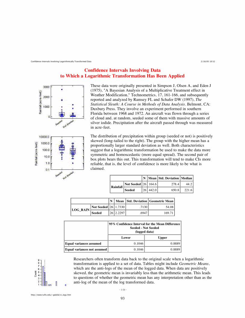
Confidence Intervals Involving Logarithmically Transformed Data 2/18/05 10:52
- 1 (3) -
http://www.tufts.edu/~gdallal/ci_logs.htm
Confidence Intervals Involving Datato Which a Logarithmic Transformation Has Been Applied
These data were originally presented in Simpson J, Olsen A, and Eden J(1975), "A Bayesian Analysis of a Multiplicative Treatment effect inWeather Modification," Technometrics, 17, 161-166, and subsequentlyreported and analyzed by Ramsey FL and Schafer DW (1997), TheStatistical Sleuth: A Course in Methods of Data Analysis. Belmont, CA:Duxbury Press. They involve an experiment performed in southernFlorida between 1968 and 1972. An aircraft was flown through a seriesof cloud and, at random, seeded some of them with massive amounts ofsilver iodide. Precipitation after the aircraft passed through was measuredin acre-feet.
The distribution of precipitation within group (seeded or not) is positivelyskewed (long-tailed to the right). The group with the higher mean has aproportionally larger standard deviation as well. Both characteristicssuggest that a logarithmic transformation be used to make the data moresymmetric and homoscedastic (more equal spread). The second pair ofbox plots bears this out. This transformation will tend to make CIs morereliable, that is, the level of confidence is more likely to be what isclaimed.
N Mean Std. Deviation MedianNot Seeded 26 164.6 278.4 44.2
RainfallSeeded 26 442.0 650.8 221.6
N Mean Std. Deviation Geometric MeanNot Seeded 26 1.7330 .7130 54.08
LOG_RAINSeeded 26 2.2297 .6947 169.71
95% Confidence Interval for the Mean DifferenceSeeded - Not Seeded
(logged data)Lower Upper
Equal variances assumed 0.1046 0.8889
Equal variances not assumed 0.1046 0.8889
Researchers often transform data back to the original scale when a logarithmictransformation is applied to a set of data. Tables might include Geometric Means,which are the anti-logs of the mean of the logged data. When data are positivelyskewed, the geometric mean is invariably less than the arithmetic mean. This leadsto questions of whether the geometric mean has any interpretation other than as theanti-log of the mean of the log transformed data.
93
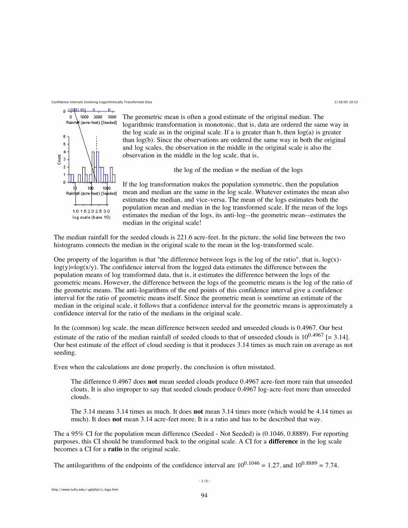
Confidence Intervals Involving Logarithmically Transformed Data 2/18/05 10:52
- 2 (3) -
http://www.tufts.edu/~gdallal/ci_logs.htm
The geometric mean is often a good estimate of the original median. Thelogarithmic transformation is monotonic, that is, data are ordered the same way inthe log scale as in the original scale. If a is greater than b, then log(a) is greaterthan log(b). Since the observations are ordered the same way in both the originaland log scales, the observation in the middle in the original scale is also theobservation in the middle in the log scale, that is,
the log of the median = the median of the logs
If the log transformation makes the population symmetric, then the populationmean and median are the same in the log scale. Whatever estimates the mean alsoestimates the median, and vice-versa. The mean of the logs estimates both thepopulation mean and median in the log transformed scale. If the mean of the logsestimates the median of the logs, its anti-log--the geometric mean--estimates themedian in the original scale!
The median rainfall for the seeded clouds is 221.6 acre-feet. In the picture, the solid line between the twohistograms connects the median in the original scale to the mean in the log-transformed scale.
One property of the logarithm is that "the difference between logs is the log of the ratio", that is, log(x)-log(y)=log(x/y). The confidence interval from the logged data estimates the difference between thepopulation means of log transformed data, that is, it estimates the difference between the logs of thegeometric means. However, the difference between the logs of the geometric means is the log of the ratio ofthe geometric means. The anti-logarithms of the end points of this confidence interval give a confidenceinterval for the ratio of geometric means itself. Since the geometric mean is sometime an estimate of themedian in the original scale, it follows that a confidence interval for the geometric means is approximately aconfidence interval for the ratio of the medians in the original scale.
In the (common) log scale, the mean difference between seeded and unseeded clouds is 0.4967. Our bestestimate of the ratio of the median rainfall of seeded clouds to that of unseeded clouds is 100.4967 [= 3.14].Our best estimate of the effect of cloud seeding is that it produces 3.14 times as much rain on average as notseeding.
Even when the calculations are done properly, the conclusion is often misstated.
The difference 0.4967 does not mean seeded clouds produce 0.4967 acre-feet more rain that unseededclouts. It is also improper to say that seeded clouds produce 0.4967 log-acre-feet more than unseededclouds.
The 3.14 means 3.14 times as much. It does not mean 3.14 times more (which would be 4.14 times asmuch). It does not mean 3.14 acre-feet more. It is a ratio and has to be described that way.
The a 95% CI for the population mean difference (Seeded - Not Seeded) is (0.1046, 0.8889). For reportingpurposes, this CI should be transformed back to the original scale. A CI for a difference in the log scalebecomes a CI for a ratio in the original scale.
The antilogarithms of the endpoints of the confidence interval are 100.1046 = 1.27, and 100.8889 = 7.74.
94
Confidence Intervals Involving Logarithmically Transformed Data 2/18/05 10:52
- 3 (3) -
http://www.tufts.edu/~gdallal/ci_logs.htm
Thus, the report would read: "The geometric mean of the amount of rain produced by a seeded cloud is 3.14times as much as that produced by an unseeded cloud (95% CI: 1.27 to 7.74 times as much)." If the loggeddata have a roughly symmetric distribution, you might go so far as to say,"The median amount of rain...isapproximately..."
Comment: The logarithm is the only transformation that produces results that can be cleanly expressed interms of the original data. Other transformations, such as the square root, are sometimes used, but it isdifficult to restate their results in terms of the original data.
Copyright © 2000 Gerard E. DallalLast modified: Mon Sep 30 2002 14:15:42.
95

CHAPTER 2. INTRODUCTION TO STATISTICS
2.9 Standard deviations and standard errors revisited
The use of standard deviations and standard errors in reports and publications can be confusing. Hereare some typical questions asked by students about these two concepts.
I am confused about why different graphs in different publication display the mean ± 1standard deviation; the mean ± 2 standard deviations; the mean ± 1 se; or the mean ± 2 se.When should each graph be used?
What is the difference between a box-plot; ±2se; and ± 2 standard deviations?
The foremost distinction between the use of standard deviation and standard errors can be made asfollows:
Standard deviations should be used when information about INDIVIDUAL observations isto be conveyed; standard errors should be used when information about the precision of anestimate is to be conveyed.
There are in fact, several common types of graphs that can be used to display the distribution ofthe INDIVIDUAL data values. Common displays from "closest to raw data" to "based on summarystatistics" are:
• dot plots
• stem and leaf plots
• histograms
• box plots
• mean ± 1 std dev. NOTE this is NOT the same as the estimate ± 1 se
• mean ± 2 std dev. NOTE this is NOT the same as the estimate ± 2 se
The dot plot is a simple plot of the actual raw data values (e.g. that seen in JMP when the Analyze->Fit Y-by-X platform is invoked. It is used to check for outliers and other unusual points. Often jitteringis used to avoid overprinting any duplicate data points. It useful for up to about 100 data points. Here isan example of a dot plot of air quality data in several years:
c©2019 Carl James Schwarz 96 2019-11-04
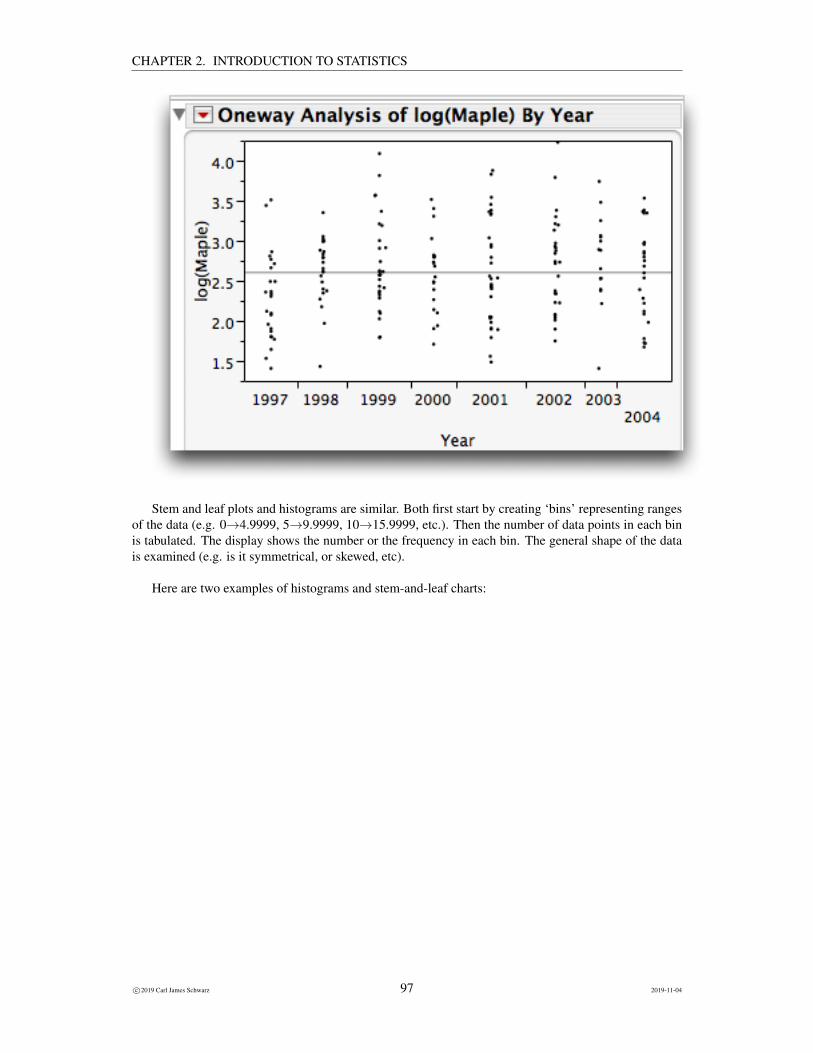
CHAPTER 2. INTRODUCTION TO STATISTICS
Stem and leaf plots and histograms are similar. Both first start by creating ‘bins’ representing rangesof the data (e.g. 0→4.9999, 5→9.9999, 10→15.9999, etc.). Then the number of data points in each binis tabulated. The display shows the number or the frequency in each bin. The general shape of the datais examined (e.g. is it symmetrical, or skewed, etc).
Here are two examples of histograms and stem-and-leaf charts:
c©2019 Carl James Schwarz 97 2019-11-04
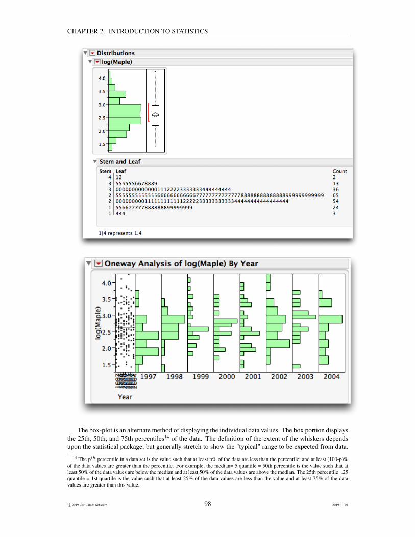
CHAPTER 2. INTRODUCTION TO STATISTICS
The box-plot is an alternate method of displaying the individual data values. The box portion displaysthe 25th, 50th, and 75th percentiles14 of the data. The definition of the extent of the whiskers dependsupon the statistical package, but generally stretch to show the "typical" range to be expected from data.
14 The pth percentile in a data set is the value such that at least p% of the data are less than the percentile; and at least (100-p)%of the data values are greater than the percentile. For example, the median=.5 quantile = 50th percentile is the value such that atleast 50% of the data values are below the median and at least 50% of the data values are above the median. The 25th percentile=.25quantile = 1st quartile is the value such that at least 25% of the data values are less than the value and at least 75% of the datavalues are greater than this value.
c©2019 Carl James Schwarz 98 2019-11-04
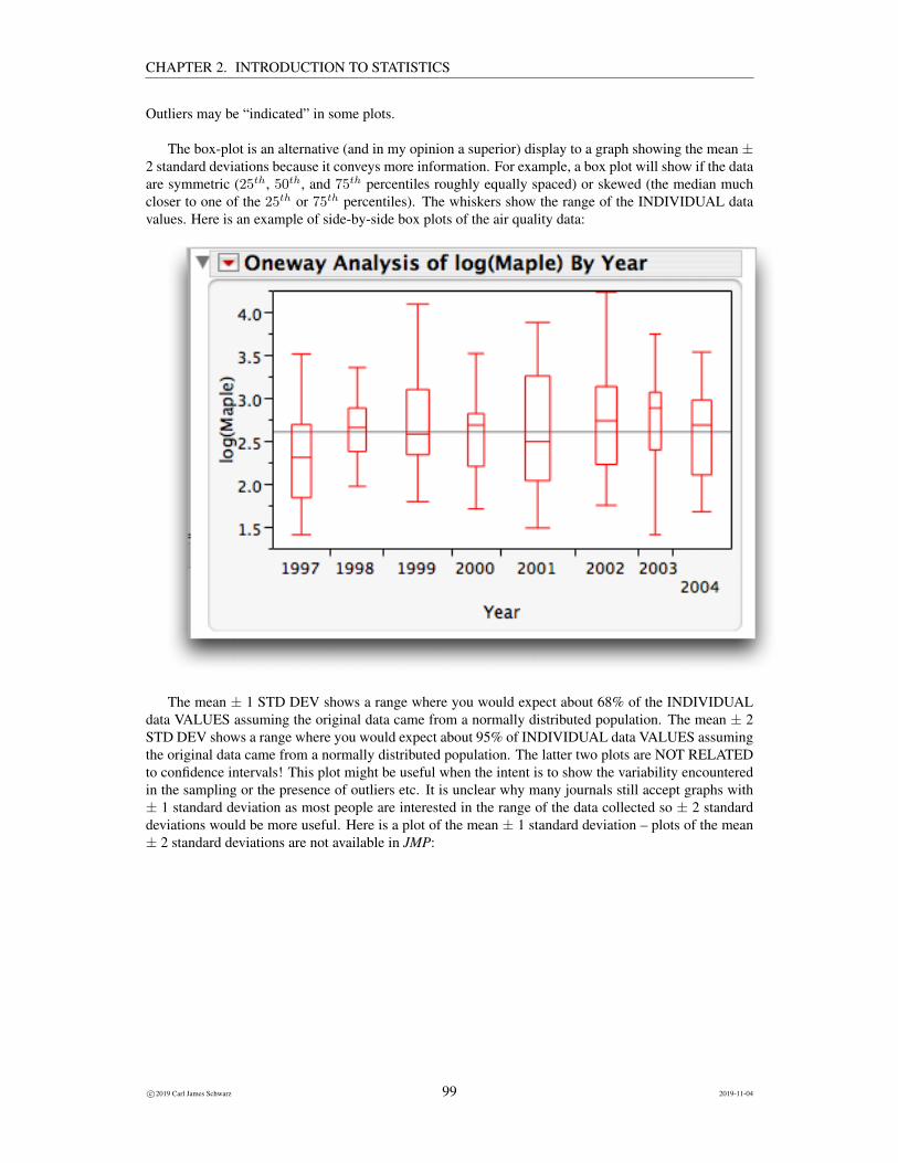
CHAPTER 2. INTRODUCTION TO STATISTICS
Outliers may be “indicated” in some plots.
The box-plot is an alternative (and in my opinion a superior) display to a graph showing the mean ±2 standard deviations because it conveys more information. For example, a box plot will show if the dataare symmetric (25th, 50th, and 75th percentiles roughly equally spaced) or skewed (the median muchcloser to one of the 25th or 75th percentiles). The whiskers show the range of the INDIVIDUAL datavalues. Here is an example of side-by-side box plots of the air quality data:
The mean ± 1 STD DEV shows a range where you would expect about 68% of the INDIVIDUALdata VALUES assuming the original data came from a normally distributed population. The mean ± 2STD DEV shows a range where you would expect about 95% of INDIVIDUAL data VALUES assumingthe original data came from a normally distributed population. The latter two plots are NOT RELATEDto confidence intervals! This plot might be useful when the intent is to show the variability encounteredin the sampling or the presence of outliers etc. It is unclear why many journals still accept graphs with± 1 standard deviation as most people are interested in the range of the data collected so ± 2 standarddeviations would be more useful. Here is a plot of the mean ± 1 standard deviation – plots of the mean± 2 standard deviations are not available in JMP:
c©2019 Carl James Schwarz 99 2019-11-04
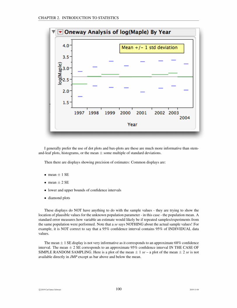
CHAPTER 2. INTRODUCTION TO STATISTICS
I generally prefer the use of dot plots and bax-plots are these are much more informative than stem-and-leaf plots, histograms, or the mean ± some multiple of standard deviations.
Then there are displays showing precision of estimates: Common displays are:
• mean ± 1 SE
• mean ± 2 SE
• lower and upper bounds of confidence intervals
• diamond plots
These displays do NOT have anything to do with the sample values - they are trying to show thelocation of plausible values for the unknown population parameter - in this case - the population mean. Astandard error measures how variable an estimate would likely be if repeated samples/experiments fromthe same population were performed. Note that a se says NOTHING about the actual sample values! Forexample, it is NOT correct to say that a 95% confidence interval contains 95% of INDIVIDUAL datavalues.
The mean± 1 SE display is not very informative as it corresponds to an approximate 68% confidenceinterval. The mean ± 2 SE corresponds to an approximate 95% confidence interval IN THE CASE OFSIMPLE RANDOM SAMPLING. Here is a plot of the mean ± 1 se – a plot of the mean ± 2 se is notavailable directly in JMP except as bar above and below the mean.
c©2019 Carl James Schwarz 100 2019-11-04

CHAPTER 2. INTRODUCTION TO STATISTICS
Alternatively, JMP can plot confidence interval diamonds.
c©2019 Carl James Schwarz 101 2019-11-04
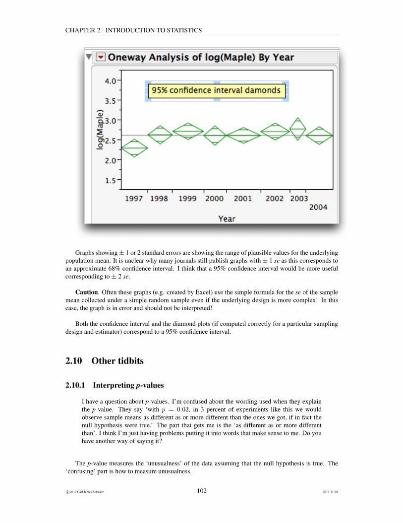
CHAPTER 2. INTRODUCTION TO STATISTICS
Graphs showing± 1 or 2 standard errors are showing the range of plausible values for the underlyingpopulation mean. It is unclear why many journals still publish graphs with ± 1 se as this corresponds toan approximate 68% confidence interval. I think that a 95% confidence interval would be more usefulcorresponding to ± 2 se.
Caution. Often these graphs (e.g. created by Excel) use the simple formula for the se of the samplemean collected under a simple random sample even if the underlying design is more complex! In thiscase, the graph is in error and should not be interpreted!
Both the confidence interval and the diamond plots (if computed correctly for a particular samplingdesign and estimator) correspond to a 95% confidence interval.
2.10 Other tidbits
2.10.1 Interpreting p-values
I have a question about p-values. I’m confused about the wording used when they explainthe p-value. They say ‘with p = 0.03, in 3 percent of experiments like this we wouldobserve sample means as different as or more different than the ones we got, if in fact thenull hypothesis were true.’ The part that gets me is the ‘as different as or more differentthan’. I think I’m just having problems putting it into words that make sense to me. Do youhave another way of saying it?
The p-value measures the ‘unusualness’ of the data assuming that the null hypothesis is true. The‘confusing’ part is how to measure unusualness.
c©2019 Carl James Schwarz 102 2019-11-04
CHAPTER 2. INTRODUCTION TO STATISTICS
For example; is a person 7 ft (about 2 m) unusually tall? Yes, because only a small fraction of peopleare AS TALL OR TALLER.
Now if the hypothesis is 2-sided, both small and large values of the sample mean (relative to thehypothesized value) are unusual. For example, suppose that null hypothesis is that the mean amount inbottles of pop is 250 mL. We would be very surprised if the sample mean was very small (e.g. 150 mL)or very large (e.g. 350 mL).
That is why, for a two-sided test, the unusualness is ‘as different or more different’. You aren’t justinterested in the probability of getting exactly 150 or 350, but rather in the probability that the samplemean is < 150 or > 350 (analogous to the probability of being 7 ft or higher).
2.10.2 False positives vs. false negatives
What is the difference between a false positive and a false negative
A false positive (Type I) error occurs if you conclude that the evidence against the hypothesis ofinterest is strong, when, in fact, the hypothesis is true. For example, in a pregnancy test, the null hypoth-esis is that the person is NOT pregnant. A false positive reading would indicate that the test indicates apregnancy, when in fact the person is not pregnant. A false negative (Type II error) occurs if insufficientevidence against the null hypothesis, in fact, the hypothesis is false. In the case of a pregnancy test, afalse negative would occur if the test indicates not pregnant, when in fact, the person is pregnant.
2.10.3 Specificity/sensitivity/power
Please clarify specificity/sensitivity/power of a test. Are they the same?
The power and sensitivity are two terms for the ability to find sufficient evidence against the the nullhypothesis when, in fact, the null hypothesis is false. For example, a pregnancy test with a 99that the testcorrectly identifies a pregnancy when in fact the person is pregnant.
The specificity of a test indicates the ability to NOT find evidence against the null hypothesis whenthe null hypothesis is true - the opposite of a Type I error. A pregnancy test would have high specificityif it rarely declares a pregnancy for a non-pregnant person.
c©2019 Carl James Schwarz 103 2019-11-04