CHAPTER Advanced Issues in Cash Management …...CHAPTER28 Advanced Issues in Cash Management and Inventory Control T his chapter provides detailed coverage of several working capital

C H A P T E R28Advanced Issues inCash Management andInventory Control

This chapter provides detailed coverage of several working capital topics,including (1) the target cash balance, (2) inventory control systems,(3) accounting treatments for inventory, and (4) the EOQ model.

© Adalberto Rios Szalay/Sexto Sol/Getty Images

1

© 2014 Cengage Learning. All Rights Reserved. May not be scanned, copied or duplicated, or posted to a publicly accessible website, in whole or in part.

28-1 The Concept of Zero Working CapitalAt first glance, it might seem that working capital management is not as important ascapital budgeting, dividend policy, and other decisions that determine a firm’s long-termdirection. However, in today’s world of intense global competition, working capitalmanagement is receiving increasing attention from managers striving for peak efficiency.In fact, the goal of many leading companies today is zero working capital. Proponents ofthe zero working capital concept claim that a movement toward this goal not onlygenerates cash but also speeds up production and helps businesses make more timelydeliveries and operate more efficiently. The concept has its own definition of workingcapital: Inventories + Receivables − Payables. The rationale here is (1) that inventories andreceivables are the keys to making sales, but (2) that inventories can be financed bysuppliers through accounts payable.

Companies generally use about 20 cents of working capital for each dollar of sales. So,on average, working capital is turned over five times per year. Reducing working capitaland thus increasing turnover has two major financial benefits. First, every dollar freed upby reducing inventories or receivables, or by increasing payables, results in a one-timecontribution to cash flow. Second, a movement toward zero working capital permanentlyraises a company’s earnings. Like all capital, funds invested in working capital cost money,so reducing those funds yields permanent savings in capital costs. In addition to thefinancial benefits, reducing working capital forces a company to produce and deliverfaster than its competitors, which helps it gain new business and charge premium pricesfor providing good services. As inventories disappear, warehouses can be sold off, bothlabor and handling equipment needs are reduced, and obsolete and/or out-of-style goodsare minimized.

The most important factor in moving toward zero working capital is increased speed. Ifthe production process is fast enough, companies can produce items as they are orderedrather than having to forecast demand and build up large inventories that are managed bybureaucracies. The best companies are able to start production after an order is receivedyet still meet customer delivery requirements. This system is known as demand flow, ordemand-based management, and it builds on the just-in-time method of inventory controldiscussed later in this chapter. However, demand flow management is broader than just-in-time, because it requires that all elements of a production system operate quickly andefficiently.

Achieving zero working capital requires that every order and part move at max-imum speed, which generally means replacing paper with electronic data. Then,orders streak from the processing department to the plant, where flexible productionlines produce each product every day and finished goods flow directly from theproduction line onto waiting trucks or rail cars. Instead of cluttering plants orwarehouses with inventories, products move directly into the pipeline. As efficiencyrises, working capital dwindles.

Clearly, it is not possible for most firms to achieve zero working capital and perfectlyefficient production. Still, a focus on minimizing cash, receivables, and inventories whilemaximizing payables will help a firm lower its investment in working capital and achievefinancial and production economies.

S E L F - T E S T

What is the basic idea of zero working capital, and how is working capital defined

for this purpose?

r e s o u r c eThe textbook’s Web sitecontains an Excel file thatwill guide you through thechapter’s calculations. Thefile for this chapter is Ch28

Tool Kit.xls, and we

encourage you to open the

file and follow along as you

read the chapter.

2 C h a p t e r 2 8 Advanced Issues in Cash Management and Inventory Control


28-2 Setting the Target Cash BalanceRecall from Chapter 16 that firms hold cash balances primarily for two reasons: to pay fortransactions they must make in their day-to-day operations and to maintain compensatingbalances that banks may require in return for loans. In addition, firms maintain additionalcash balances as a precaution against unforeseen fluctuations in cash flows and in order totake advantage of trade discounts. Given that cash is necessary for these purposes but isalso a nonearning asset, the primary goal of cash management is to minimize the amountof cash a firm holds while maintaining a sufficient target cash balance to conduct business.

In Chapter 16, when we discussed Educational Products Corporation’s cash budget, wetook as a given the $10 million target cash balance. We also discussed how lockboxes,synchronizing inflows and outflows, and float can reduce the required cash balance. Nowwe consider how target cash balances are set in practice.

Note that (1) cash per se earns no return, (2) cash is an asset that appears on the leftside of the balance sheet, (3) cash holdings must be financed by raising either debt orequity, and (4) both debt and equity capital have a cost. If cash holdings could be reducedwithout hurting sales or other aspects of a firm’s operations, then this reduction wouldpermit a reduction in either debt or equity or both, which would increase the return oncapital and thus boost the value of the firm’s stock. Therefore, the general operating goal ofthe cash manager is to minimize the amount of cash held subject to the constraint thatenough cash be held to enable the firm to operate efficiently.

For most firms, cash as a percentage of assets and/or sales has declined sharply over thelast couple of decades as a direct result of technological developments in computers andtelecommunications. Years ago, it was difficult to move money from one location toanother, and it was also difficult to forecast exactly how much cash would be needed indifferent locations at different points in time. As a result, firms had to hold relatively large“safety stocks” of cash to be sure they had enough when and where it was needed. Also,they held relatively large amounts of short-term securities as a backup, and they also hadbackup lines of credit that permitted them to borrow on short notice to build up the cashaccount if it became depleted.

Think about how computers and telecommunications now affect the situation. With a goodcomputer system tied together with good telecommunications links, a company can get real-time information on its cash balances regardless of whether it operates in a single location or allover the world. Furthermore, it can use statistical procedures to forecast cash inflows andoutflows, and good forecasts reduce the need for safety stocks. Finally, improvements intelecommunications systems make it possible for a treasurer to replenish the firm’s cashaccounts within minutes simply by calling a lender and stating that the firm wants to borrowa given amount under its line of credit. The lender then wires the funds to the desired location.Similarly, marketable securities can be sold with close to the same speed and with the sameminimal transactions costs. This trend toward lower cash levels, however, was reversed in thewake of the financial crisis in 2008 and 2009 when firms found it difficult to obtain or renewlines of credit. As they became profitable moving out of the accompanying recession, manyfirms have squirreled away relatively larger amounts of cash as a safeguard against turmoil in thebanking industry.

Super Cell, a provider of cell phone services, can be used to illustrate the impact ofcomputers and high-speed telecommunications on cash management. Super Cellknows exactly how much it must pay and when, and it can forecast quite accuratelywhen it will receive checks. For example, the treasurer of Super Cell’s Floridaoperation knows when the major employers in Tampa pay their workers and howlong after that people generally pay their phone bills. Armed with this information,Super Cell’s Florida treasurer can forecast with great accuracy any cash surpluses or

C h a p t e r 2 8 Advanced Issues in Cash Management and Inventory Control 3


deficits on a daily basis. Of course, no forecast will be exact, so slight overages orunderages will occur. But this presents no problem. The treasurer knows by 11 a.m.the checks that must be covered by 4 p.m. that day, how much cash has come in, andconsequently how much of a cash surplus or deficit will exist. Then, with a singlephone call, the company borrows to cover any deficit or buys securities (or pays offoutstanding loans) with any surplus. Thus, Super Cell can maintain cash balances thatare very close to zero, a situation that would have been impossible a few years ago.

Today, cash management in reasonably sophisticated firms is largely a job forsystems people. Except for the very largest firms, it is generally most efficient to havea bank handle the actual operations of the cash management system. When it comesto operating a cash management system, banks have extensive experience and are ableto capture economies of scale that are unobtainable by individual nonfinancial firms.Also, many banks are willing and able to offer such services, so competition hasdriven the cost of cash management down to a reasonable level. Still, it is essentialthat corporate treasurers know enough about cash management procedures to be ableto negotiate and then work with the banks to ensure that they get the best price(interest rate) on credit lines, the best yield on short-term investments, and a reason-able cost for other banking services. To provide perspective on these issues, we nextdiscuss a theoretical model for cash balances as well as a practical approach to settingthe target cash balance.

28-2a The Baumol ModelWilliam Baumol first noted that cash balances are, in many respects, similar to inventoriesand that the EOQ inventory model, which will be developed in a later section, can be usedto establish a target cash balance.1 Baumol’s model assumes that the firm uses cash at asteady, predictable rate—say, $1,000,000 per week—and that the firm’s cash inflows fromoperations also occur at a steady, predictable rate—say, $900,000 per week. Therefore, thefirm’s net cash outflows, or net need for cash, also occur at a steady rate—in this case,$100,000 per week.2 Under these steady-state assumptions, the firm’s cash position willresemble the situation shown in Figure 28-1.

If our illustrative firm started at Time 0 with a cash balance of C = $300,000 andif its outflows exceeded its inflows by $100,000 per week, then its cash balancewould drop to zero at the end of Week 3 and its average cash balance would beC/2 = $300,000/2 = $150,000. Therefore, at the end of Week 3, the firm would haveto replenish its cash balance by selling marketable securities (if it had any) or byborrowing.

If C were set at a higher level—say, $600,000—then the cash supply would last longer(6 weeks) and the firm would have to sell securities (or borrow) less frequently. However,its average cash balance would rise from $150,000 to $300,000. Brokerage or some othertype of transaction costs must be incurred to sell securities (or to borrow), so holdinglarger cash balances will lower the transaction costs associated with obtaining cash. On theother hand, cash provides no income, so larger average cash balances entail a higheropportunity cost, which is the return that could have been earned on securities or other

1William J. Baumol, “The Transactions Demand for Cash: An Inventory Theoretic Approach,” Quarterly Journalof Economics, November 1952, pp. 545–556.2Our hypothetical firm is experiencing a $100,000 weekly cash shortfall, but this does not necessarily imply it isheaded for bankruptcy. The firm could, for example, be highly profitable and be enjoying high earnings yet beexpanding so rapidly that it experiences chronic cash shortages that must be made up by borrowing or by sellingcommon stock. Or the firm could be in the construction business and therefore receive major cash inflows atwidely spaced intervals but still have net cash outflows of $100,000 per week between these inflows.



assets held in lieu of cash. Thus, we have the situation graphed in Figure 28-2. Theoptimal cash balance is found by using the following variables and equations:

C = Amount of cash raised by selling marketable securities or by borrowing.

C/2 = Average cash balance.

C* = Optimal amount of cash to be raised by selling marketable securities orby borrowing.

C*/2 = Optimal average cash balance.

F = Fixed costs of selling securities or of obtaining a loan.

T = Total amount of net new cash needed for transactions during the entireperiod (usually a year).

r = Opportunity cost of holding cash, set equal to either the rate of returnforgone on marketable securities or the cost of borrowing to hold cash.

The total costs of cash balances consist of holding (or opportunity) costs plus transac-tions costs:3

Total costs ¼ Holding costs þ Transactions costs

¼ Average cashbalance

� �Opportunitycost rate

� �þ Number of

transactions

� �Cost per

transaction

� �

¼ C2ðrÞ þ T

CðFÞ

(28-1)

FIGURE 28-1

Cash Balances under the Baumol Model’s Assumptions

0 1 2 3 4 5 6 7 8 9 10 11 12

Cash Balances ($)

Weeks

Maximum Cash = C

Average Cash = C/2

Ending Cash = 0

© Cengage Learning 2014

3Total costs can be expressed on either a before-tax or an after-tax basis. Both methods lead to the sameconclusions regarding target cash balances and comparative costs. For simplicity, we present the model here on abefore-tax basis.



The minimum total costs are achieved when C is set equal to C*, the optimal cashtransfer. The value of C* is found as follows:4

C� ¼ffiffiffiffiffiffiffiffiffiffiffiffiffiffiffiffiffi2ðFÞðTÞ

r

r(28-2)

Equation 28-2 is the Baumol model for determining optimal cash balances. Toillustrate its use, suppose F = $150, T = 52 weeks × $100,000/week = $5,200,000,and r = 15% = 0.15. Then

C� ¼ffiffiffiffiffiffiffiffiffiffiffiffiffiffiffiffiffiffiffiffiffiffiffiffiffiffiffiffiffiffiffiffiffiffiffiffiffiffiffiffiffiffi2ð$150Þð$5;200;000Þ

0:15

r¼ $101;980

Therefore, the firm should sell securities (or borrow if it does not hold securities) in theamount of $101,980 when its cash balance approaches zero, thus building its cash balanceback up to $101,980. Dividing T by C* yields the number of transactions per year:$5,200,000/$101,980 = 50.99 ≈ 51, or about once a week. The firm’s average cash balanceis $101,980/2 = $50,990 ≈ $51,000.

Note that the optimal cash balance increases less than proportionately with increases inthe amount of cash needed for transactions. For example, if the firm’s size, and

FIGURE 28-2

Determination of the Target Cash Balance

0

Transactions Costs

Total Costs of Holding Cash

C*Optimal

Cash Transfer

Cash Transferred ($)

Costs of Holding Cash ($)

Opportunity Costs


4Equation 28-1 is differentiated with respect to C. The derivative is set equal to zero, and we then solve for C = C*

to derive Equation 28-2. This model, applied to inventories and called the EOQ model, is discussed further in alater section.



consequently its net new cash needs, doubled from $5,200,000 to $10,400,000 per year,then average cash balances would increase by only 41%, from $51,000 to $72,000. Thissuggests that there are economies of scale in holding cash balances, and this, in turn, giveslarger firms an edge over smaller ones.5

Of course, the firm would probably want to hold a safety stock of cash designed toreduce the probability of a cash shortage. However, if the firm is able to sell securities or toborrow on short notice—and most larger firms can do so in a matter of minutes simply bymaking a telephone call—then the safety stock can be quite low.

The Baumol model is obviously simplistic. Most important, it assumes relatively stable,predictable cash inflows and outflows, and it does not take into account seasonal orcyclical trends. Other models have been developed to deal both with uncertainty and withtrends, but all of them have limitations and are more useful as conceptual models than foractually setting target cash balances.

28-2b Monte Carlo SimulationAlthough the Baumol model and other theoretical models provide insights into theoptimal cash balance, they are generally not practical for actual use. Rather, firmsgenerally set their target cash balances based on some “safety stock” of cash that holdsthe risk of running out of money to some acceptably low level. One commonly usedprocedure is Monte Carlo simulation. To illustrate, consider the cash budget for Educa-tional Products Corporation (EPC) presented in Figure 16-5 in Chapter 16. Sales andcollections are the driving forces in the cash budget and, of course, are subject touncertainty. In the cash budget, we used expected values for sales and collections as wellas for all other cash flows. However, it would be relatively easy to use Monte Carlosimulation, first discussed in Chapter 11, to introduce uncertainty. If the cash budget wereconstructed using a spreadsheet program with Monte Carlo add-in software, then the keyuncertain variables could be specified as continuous probability distributions rather thanpoint values.

The end result of the simulation would be a distribution for each month’s net cash flowinstead of the single values shown on Row 165 of Figure 16-5. Suppose September’s netcash flow distribution looked like this (in millions):

September Net

Cash Flow

Probability of This

Cash Flow or Less

−$208 10%

−200 20

−193 30

−187 40

−182 Expected CF 50

−177 60

−171 70

−164 80

−156 90

5This edge may, of course, be more than offset by other factors—after all, cash management is only one aspect ofrunning a business.



Now suppose EPC’s managers want to be 90% confident that the firm will not run outof cash during September, because they don’t want to borrow to cover any shortfall. Theywould set the beginning-of-month target balance at $200 million, well above the currenttarget balance of $10 million, because there is only a 10% probability that September’scash flow will be worse than a $200 million outflow. With a balance of $200 million at thebeginning of the month, there would be only a 10% chance that EPC would run out ofcash during September. Of course, Monte Carlo simulation could be applied to theremaining months in the Figure 16-5 cash budget, and the amounts so obtained to matcha given confidence level could be used to set each month’s target cash balance instead ofusing a fixed target across all months.

The same type of analysis could be used to determine the amount of short-term securitiesto hold or the size of a requested line of credit. Of course, as in all simulations, the hard part isestimating the probability distributions for sales, collections, and the other highly uncertainvariables. If these inputs are not good representations of the actual uncertainty facing thefirm, then the resulting target balances will not offer the protection against cash shortagesimplied by the simulation. There is no substitute for experience, and cash managers willadjust the target balances obtained by Monte Carlo simulation based on their own judgment.

S E L F - T E S T

How has technology changed the way target cash balances are set?

What is the Baumol model, and how is it used?

Explain how Monte Carlo simulation can be used to help set a firm’s target cash

balance.

28-3 Inventory Control SystemsInventory management requires the establishment of an inventory control system. Inven-tory control systems run the gamut from very simple to extremely complex, depending onthe size of the firm and the nature of its inventory. For example, one simple controlprocedure is the red-line method—inventory items are stocked in a bin, a red line isdrawn around the inside of the bin at the level of the reorder point, and the inventoryclerk places an order when the red line shows. The two-bin method has inventory itemsstocked in two bins. When the working bin is empty, an order is placed and inventory isdrawn from the second bin. These procedures work well for parts such as bolts in amanufacturing process or for many items in retail businesses.

28-3a Computerized SystemsMost companies today employ computerized inventory control systems. The computerstarts with an inventory count in memory. As withdrawals are made, they are recorded by thecomputer, and the inventory balance is revised. When the reorder point is reached, thecomputer automatically places an order, and when the order is received, the recorded balanceis increased. As we noted earlier, retailers such as Walmart have carried this system quite far:Each item has a bar code and, as an item is checked out, the code is read, a signal is sent to thecomputer, and the inventory balance is adjusted at the same time the price is fed into the cashregister tape. When the balance drops to the reorder point, an order is placed. In Walmart’scase, the order goes directly from its computers to those of its suppliers.



A good inventory control system is dynamic, not static. A company such as Walmartor General Motors stocks hundreds of thousands of different items. The sales (or use) ofindividual items can rise or fall quite separately from rising or falling overall corporatesales. As the usage rate for an individual item begins to rise or fall, the inventory managermust adjust its balance to avoid running short or ending up with obsolete items. Ifthe change in the usage rate appears to be permanent, then the safety stock levelshould be reconsidered and the computer model used in the control process should bereprogrammed.

28-3b Just-in-Time SystemsAn approach to inventory control called the just-in-time (JIT) system was developed byJapanese firms but is now used throughout the world. Toyota provides a good exampleof the just-in-time system. Many of Toyota’s suppliers are located near its factories.Delivery of components is tied to the speed of the assembly line, and parts are generallydelivered no more than a few hours before they are used. The just-in-time systemreduces the need for Toyota and other manufacturers to carry large inventories, but itrequires a great deal of coordination between the manufacturer and its suppliers—bothin the timing of deliveries and the quality of the parts. The component parts mustbe perfect, because a few bad parts could stop the entire production line. Therefore,JIT inventory management has been developed in conjunction with total qualitymanagement (TQM).

The close coordination required between the parties using JIT procedures has led to anoverall reduction of inventory throughout the production–distribution system and to ageneral improvement in economic efficiency. This point is borne out by economicstatistics, which show that inventory as a percentage of sales has been declining sincethe use of just-in-time procedures began. Also, with smaller inventories in the system,economic recessions have become shorter and less severe.

28-3c OutsourcingAnother important development related to inventory is outsourcing, which is the practiceof purchasing components rather than making them in-house. Thus, GM has beenmoving toward buying radiators, axles, and other parts from suppliers rather than makingthem itself, so it has been increasing its use of outsourcing. Outsourcing is often combinedwith just-in-time systems to reduce inventory levels. However, perhaps the major reasonfor outsourcing has nothing to do with inventory policy: A bureaucratic, unionizedcompany like GM can often buy parts from a smaller, nonunionized supplier at a lowercost than it can make them itself.

28-3d The Relationship between Production Schedulingand Inventory LevelsA final point relating to inventory levels is the relationship between production schedulingand inventory levels. For example, a greeting card manufacturer has highly seasonal sales.Such a firm could produce on a steady, year-round basis, or it could let production riseand fall with sales. If it established a level production schedule, its inventory would risesharply during periods when sales were low and then decline during peak sales periods,but its average inventory would be substantially higher than if production rose and fellwith sales.



Our discussions of just-in-time systems, outsourcing, and production scheduling allpoint out the necessity of coordinating inventory policy with manufacturing/procurementpolicies. Companies try to minimize total production and distribution costs, and inventorycosts are just one part of total costs. Still, they are an important cost, and financialmanagers should be aware of the determinants of inventory costs and how those costscan be minimized.

S E L F - T E S T

Describe some inventory control systems that are used in practice.

What are just-in-time systems? What are their advantages? Why is quality

especially important if a JIT system is used?

What is outsourcing?

Describe the relationship between production scheduling and inventory levels.

28-4 Accounting for InventoryWhen finished goods are sold, the firm must assign a cost of goods sold. The cost ofgoods sold appears on the income statement as an expense for the period, and thebalance sheet inventory account is reduced by a like amount. Four methods can be usedto value the cost of goods sold and hence to value the remaining inventory: (1) specificidentification, (2) first-in, first-out (FIFO), (3) last-in, first-out (LIFO), and (4) weightedaverage.

28-4a Specific IdentificationUnder specific identification, a unique cost is attached to each item in inventory. Then,when an item is sold, the inventory value is reduced by that specific amount. This methodis used only when the items are high cost and move relatively slowly, such as cars for anautomobile dealer.

28-4b First-In, First-Out (FIFO)In the FIFO method, the units sold during a given period are assumed to be the first unitsthat were placed in inventory. As a result, the cost of goods sold is based on the cost of theoldest inventory items, and the remaining inventory consists of the newest goods.

28-4c Last-In, First-Out (LIFO)LIFO is the opposite of FIFO. The cost of goods sold is based on the last units placed ininventory, while the remaining inventory consists of the first goods placed in inventory.Note that this is purely an accounting convention—the actual physical units sold could beeither the earlier or the later units placed in inventory, or some combination. For example,Del Monte has in its LIFO inventory accounts catsup bottled in the 1920s, but all thecatsup in its warehouses was bottled in 2012 or 2013. Note, however, that once interna-tional financial reporting standards (IFRS) are adopted for U.S. companies, LIFO account-ing for inventory will no longer be allowed. Adoption of IFRS by U.S. companies has beendelayed until at least 2015.



28-4d Weighted AverageThe weighted average method involves calculating the weighted average unit cost ofgoods available for sale from inventory; the average is then used to determine the cost ofgoods sold. This method results in a cost of goods sold and an ending inventory that fallsomewhere between the FIFO and LIFO methods.

28-4e Comparison of Inventory Accounting MethodsTo illustrate these methods and their effects on financial statements, assume that CustomFurniture Inc. manufactured five identical faux antique dining tables during a 1-yearaccounting period. During the year, a new labor contract and dramatically increasingmahogany prices caused manufacturing costs to almost double, resulting in the followinginventory costs:

There were no tables in stock at the beginning of the year, and Tables 1, 3, and 5 were soldduring the year.

If Custom used the specific identification method, then the cost of goods sold would bereported as $ 10,000 + $14,000 + $18,000 = $42,000 and the end-of-period inventory valuewould be $70,000 − $42,000 = $28,000. If Custom used the FIFO method, then its cost ofgoods sold would be $10,000 + $12,000 + $14,000 = $36,000 and ending inventory wouldbe $70,000 − $36,000 = $34,000. If Custom used the LIFO method, then its cost of goodssold would be $48,000 and its ending inventory would be $22,000. Finally, if Custom usedthe weighted average method, then its average cost per unit of inventory would be$70,000/5 = $14,000, its cost of goods sold would be 3($14,000) = $42,000, and its endinginventory would be $70,000 − $42,000 = $28,000.

If Custom’s actual sales revenues from the tables were $80,000, or an average of$26,667 per unit sold, and if its other costs were minimal, then the following tablesummarizes the effects of the four methods:

If we ignore taxes, then Custom’s cash flows would not be affected by its choice ofinventory methods, yet its balance sheet and reported profits would vary with each method.In an inflationary period such as in our example, FIFO gives the lowest cost of goods soldand thus the highest net income. FIFO also shows the highest inventory value, so itproduces the strongest apparent liquidity position as measured by net working capital orthe current ratio. On the other hand, LIFO produces the highest cost of goods sold, thelowest reported profits, and the weakest apparent liquidity position. However, when taxesare considered, LIFO provides the greatest tax deductibility and therefore results in thelowest tax burden. Consequently, after-tax cash flows are highest when LIFO is used.

Method Sales

Cost of

Goods Sold

Reported

Profit

Ending

Inventory Value

Specific identification $80,000 $42,000 $38,000 $28,000

FIFO 80,000 36,000 44,000 34,000

LIFO 80,000 48,000 32,000 22,000

Weighted average 80,000 42,000 38,000 28,000

Table Number: 1 2 3 4 5 Total

Cost: $10,000 $12,000 $14,000 $16,000 $18,000 $70,000



Of course, these results apply only to periods when costs are increasing. If costs wereconstant then all four methods would produce the same cost of goods sold, endinginventory, taxes, and cash flows. However, inflation has been a fact of life in recent years,so most firms use LIFO to take advantage of its greater tax and cash flow benefits.

S E L F - T E S T

What are the four methods used to account for inventory?

What effect does each method used have on the firm’s reported profits? On ending

inventory levels?

Which method should be used if management anticipates a period of inflation?

Why?

28-5 The Economic Ordering Quantity(EOQ) ModelAs discussed in Chapter 16, inventories are obviously necessary, but it is equally obvious that afirm’s profitability will suffer if it has too much or too little inventory. Most firms take apragmatic approach to setting inventory levels in which past experience plays a major role.However, as a starting point in the process, it is useful for managers to consider the insightsprovided by the Economic Ordering Quantity (EOQ) model. The EOQ model first specifiesthe costs of ordering and carrying inventories and then combines these costs to obtain the totalcosts associated with inventory holdings. Finally, optimization techniques are used to find theorder quantity, and hence inventory level, that minimizes total costs. Note that a third categoryof inventory costs, the costs of running short (stock-out costs), is not considered in our initialdiscussion. These costs are dealt with by adding safety stocks, as we discuss later. Similarly, weshall discuss quantity discounts in a later section. The costs that remain for consideration at thisstage are carrying costs and ordering, shipping, and receiving costs.

28-5a Carrying CostsCarrying costs generally rise in direct proportion to the average amount of inventory carried.Inventories carried, in turn, depend on the frequency with which orders are placed. Toillustrate, suppose a firm sells S units per year and places equal-sized orders N times per year;then S/N units will be purchased with each order. If the inventory is used evenly over the yearand if no safety stocks are carried, then the average inventory, A, will be

A ¼Units per order2

¼ S=N2

(28-3)

For example, if S = 120,000 units in a year and N = 4, then the firm will order 30,000 unitsat a time and its average inventory will be 15,000 units:

A ¼ S=N2

¼ 120;000=42

¼ 30;0002

¼ 15;000 units

Just after a shipment arrives, the inventory will be 30,000 units; just before the nextshipment arrives, it will be zero; and on average, 15,000 units will be carried.



Now assume the firm purchases its inventory at a price P = $2 per unit. Theaverage inventory value is thus (P)(A) = $2(15,000) = $30,000. If the firm has a costof capital of 10%, it will incur $3,000 in financing charges to carry the inventory for1 year. Further, assume that each year the firm incurs $2,000 of storage costs(space, utilities, security, taxes, and so forth), that its inventory insurance costs are$500, and that it must mark down inventories by $1,000 because of depreciation andobsolescence. The firm’s total cost of carrying the $30,000 average inventory is thus$3,000 + $2,000 + $500 + $1,000 = $6,500, and the annual percentage cost of carryingthe inventory is $6,500/$30,000 = 0.217 = 21.7%.

Defining the annual percentage carrying cost as C, we can, in general, find the annualtotal carrying cost, TCC, as the percentage carrying cost (C) multiplied by the price perunit (P) times the average number of units (A):

Total carrying cost ¼ TCC ¼ Cð Þ Pð Þ Að Þ (28-4)

In our example,

TCC ¼ 0:217ð Þ $2ð Þ 15;000ð Þ ≈ $6;500

28-5b Ordering CostsAlthough we assume that carrying costs are entirely variable and rise in direct proportionto the average size of inventories, ordering costs are often fixed. For example, the costs ofplacing and receiving an order—interoffice memos, long-distance telephone calls, settingup a production run, and taking delivery—are essentially fixed regardless of the size of anorder, so this part of inventory cost is simply the fixed cost of placing and receiving ordersmultiplied by the number of orders placed per year.6 We define the fixed costs associatedwith ordering inventories as F, and if we place N orders per year then the total orderingcost is given by Equation 28-5:

Total ordering cost ¼ TOC ¼ Fð Þ Nð Þ (28-5)

Here TOC = total ordering cost, F = fixed costs per order, and N = number of ordersplaced per year.

Equation 28-3 may be rewritten as N = S/2A and then substituted into Equation 28-5:

Total ordering cost ¼ TOC ¼ FS2A

� �(28-6)

6Note that, in reality, both carrying and ordering costs can have variable and fixed-cost elements—at least overcertain ranges of average inventory. For example, security and utilities charges are probably fixed in the short runover a wide range of inventory levels. Similarly, labor costs in receiving inventory could be tied to the quantityreceived and hence could be variable. To simplify matters, we treat all carrying costs as variable and all orderingcosts as fixed. However, if these assumptions do not fit the situation at hand, the cost definitions can be changed.For example, one could add another term for shipping costs if there are economies of scale in shipping such thatthe cost of shipping a unit is smaller if shipments are larger. However, in most situations shipping costs are notsensitive to order size, so total shipping costs are simply the shipping cost per unit times the units ordered (andsold) during the year. Under this condition, shipping costs are not influenced by inventory policy; hence theymay be disregarded for purposes of determining the optimal inventory level and the optimal order size.



To illustrate the use of Equation 28-6, let F = $100, S = 120,000 units, and A = 15,000units. Then TOC, the total annual ordering cost, is $400:

TOC ¼ $100120;00030;000

� �¼ $100 4ð Þ ¼ $400

28-5c Total Inventory CostsTotal carrying cost, TCC, as defined in Equation 28-4, and total ordering cost, TOC, asdefined in Equation 28-6, may be combined to find total inventory costs, TIC, as follows:

Total inventory costs ¼ TIC ¼ TCC þ TOC

¼ Cð Þ Pð Þ Að Þ þ FS2A

� � (28-7)

Recognizing that the average inventory carried is A = Q/2, or one-half the size of eachorder quantity, Q, we may rewrite Equation 28-7 as

TIC ¼ TCC þ TOC

¼ Cð Þ Pð Þ Q2

� �þ ðFÞ S

Q

� � (28-8)

Here we see that total carrying cost equals average inventory in units, Q/2, multiplied byunit price, P, times the percentage annual carrying cost, C. Total ordering cost equals thenumber of orders placed per year, S/Q, multiplied by the fixed cost of placing andreceiving an order, F. Finally, total inventory costs equal the sum of total carrying costplus total ordering cost. We will use this equation in the next section to develop theoptimal inventory ordering quantity.

28-5d Derivation of the EOQ ModelFigure 28-3 illustrates the basic premise on which the EOQ model is built—namely, thatsome costs rise with larger inventories while other costs decline and there is an optimalorder size (and associated average inventory) that minimizes the total costs of inventories.First, as noted earlier, the average investment in inventories depends on how frequentlyorders are placed and the size of each order—if we fill orders every day, then averageinventories will be much smaller than if we fill orders once a year. Further, as Figure 28-3shows, the firm’s carrying costs rise with larger orders; larger orders mean larger averageinventories and so warehousing costs, interest on funds tied up in inventory, insurance,and obsolescence costs will all increase. However, ordering costs decline with larger ordersand inventories; the cost of placing orders, suppliers’ production setup costs, and order-handling costs will all decline if we order infrequently and consequently hold largerquantities.

If the carrying and ordering cost curves in Figure 28-3 are added, the sumrepresents total inventory costs, TIC. The point at which the TIC is minimizedrepresents the Economic Ordering Quantity, and this, in turn, determines the optimalaverage inventory level.



The EOQ is found by differentiating Equation 28-8 with respect to ordering quantity,Q, and setting the derivative equal to zero:

dðTICÞdQ

¼ ðCÞðPÞ2

−ðFÞðSÞQ2 ¼ 0

Now, solving for Q, we obtain:

ðCÞðPÞ2

¼ ðFÞðSÞQ2

Q2 ¼ 2ðFÞðSÞðCÞðPÞ

Q ¼ EOQ ¼ffiffiffiffiffiffiffiffiffiffiffiffiffiffiffiffiffi2 Fð Þ Sð ÞCð Þ Pð Þ

s(28-9)

Here:

EOQ = Economic Ordering Quantity—the optimal quantity to be ordered each timean order is placed.

F = Fixed costs of placing and receiving an order.

S = Annual sales in units.

C = Annual carrying costs expressed as a percentage of average inventory value.

P = Purchase price the firm must pay per unit of inventory.

FIGURE 28-3

Determination of the Optimal Order Quantity

Costs of Ordering andCarrying Inventories ($)

0 EOQ Order Size (Units)

Total Inventory Costs (TIC)

Total Carrying Cost (TCC)

Total Ordering Cost (TOC)




Equation 28-9 is the EOQ model.7 The assumptions of the model, which will be relaxedshortly, include the following: (1) sales can be forecasted perfectly, (2) sales are evenlydistributed throughout the year, and (3) orders are received when expected.

28-5e EOQ Model IllustrationAs an illustration of the EOQ model, consider the following data supplied by Cotton TopsInc., a distributor of budget-priced, custom-designed T-shirts that it sells to concession-aires at various theme parks in the United States:

S = Annual sales = 26,000 shirts per year.

C = Percentage carrying cost = 25% of inventory value.

P = Purchase price per shirt = $4.92 per shirt.

F = Fixed cost per order = $1,000. Cotton Tops designs and distributes the shirts,but the actual production is done by another company. The bulk of this$1,000 cost is the labor cost for setting up the equipment for the productionrun, which the manufacturer bills separately from the $4.92 cost per shirt.

Substituting these data into Equation 28-9, we obtain an EOQ of 6,500 units:

EOQ ¼ffiffiffiffiffiffiffiffiffiffiffiffiffiffiffiffiffi2 Fð Þ Sð ÞCð Þ Pð Þ

s¼

ffiffiffiffiffiffiffiffiffiffiffiffiffiffiffiffiffiffiffiffiffiffiffiffiffiffiffiffiffiffiffiffiffiffiffiffiffiffiffiffiffi2ð Þ $1;000ð Þ 26;000ð Þ

0:25ð Þ $4:92ð Þ

s

¼ ffiffiffiffiffiffiffiffiffiffiffiffiffiffiffiffiffiffiffiffiffiffi42;276;423

p≈ 6;500 units

With an EOQ of 6,500 shirts and annual usage of 26,000 shirts, Cotton Tops will place26,000/6,500 = 4 orders per year. Note that average inventory holdings depend directly onthe EOQ. This relationship is illustrated graphically in Figure 28-4, where we see thataverage inventory = EOQ/2. Immediately after an order is received, 6,500 shirts are in stock.The usage rate, or sales rate, is 500 shirts per week (26,000/52 weeks), so inventories aredrawn down by this amount each week. Thus, the actual number of units held in inventorywill vary from 6,500 shirts just after an order is received to zero just before a new orderarrives. With a 6,500 beginning balance, a zero ending balance, and a uniform sales rate,inventories will average one-half the EOQ, or 3,250 shirts, during the year. At a cost of $4.92per shirt, the average investment in inventories will be (3,250)($4.92) ≈ $16,000. If inven-tories are financed by bank loans then the loan will vary from a high of $32,000 to a low of$0, but the average amount outstanding over the course of a year will be $16,000.

Note that the EOQ, and hence the average inventory holdings, rises with the squareroot of sales. Therefore, a given increase in sales will result in a less-than-proportionateincrease in inventories, so the inventory/sales ratio will tend to decline as a firm grows.For example, Cotton Tops’s EOQ is 6,500 shirts at an annual sales level of 26,000, and theaverage inventory is 3,250 shirts, or $16,000. However, if sales were to increase by 100% to52,000 shirts per year, then the EOQ would rise only to 9,195 units or by 41%, and the

EOQ ¼ffiffiffiffiffiffiffiffiffiffiffiffiffiffiffiffiffi2 Fð Þ Sð ÞC�

r7The EOQ model can also be written as

where C* is the annual carrying cost per unit expressed in dollars.



average inventory would rise by this same percentage. This suggests there are economiesof scale in holding inventories.8

Finally, look at Cotton Tops’s total inventory costs for the year, assuming thatthe EOQ is ordered each time. Using Equation 28-8, we find that total inventory costsare $8,000:

TIC ¼ TCC þ TOC

¼ Cð Þ Pð Þ Q2

� �þ Fð Þ S

Q

� �

¼ 0:25 $4:92ð Þ 6;5002

� �þ $1;000ð Þ 26;000

6;500

� �≈ $4;000 þ $4;000 ¼ $8;000

Note these two points: (1) The $8,000 total inventory cost represents the total of carryingcosts and ordering costs, but this amount does not include the 26,000 ($4.92) = $127,920annual purchasing cost of the inventory itself. (2) As we see both in Figure 28-3 and in thecalculation above, at the EOQ, total carrying cost (TCC) equals total ordering cost (TOC).This property is not unique to our Cotton Tops illustration; it always holds.

FIGURE 28-4

Inventory Position without Safety Stock

2 4 6 8 10 12 14 16 18 20 22 24 26 280

1

2

3

4

5

6

7

8

6.5

Order Lead Time = 2 Weeks

EOQ

Units(in Thousands)

Maximum Inventory= 6,500 = EOQ

Slope = Sales Rate = 500 Shirts per Week

AverageInventory= 3,250

Order Point= 1,000

Weeks


8Note, however, that these scale economies relate to each particular item, not to the entire firm. Thus, a largedistributor with $500 million of sales might have a higher inventory/sales ratio than a much smaller distributor ifthe small firm has only a few items with high sales volume and the large firm distributes a great many low-volume items.



28-5f Setting the Order PointIf a 2-week lead time is required for production and shipping, what is Cotton Tops’s orderpoint level? Cotton Tops sells 26,000/52 = 500 shirts per week. Thus, if a 2-week lagoccurs between placing an order and receiving goods, Cotton Tops must place the orderwhen there are 2(500) = 1,000 shirts on hand. During the 2-week production and shippingperiod, the inventory balance will continue to decline at the rate of 500 shirts per week,and the inventory balance will hit zero just as the order of new shirts arrives.

If Cotton Tops knew for certain that both the sales rate and the order lead time wouldnever vary, then it could operate exactly as shown in Figure 28-4. However, sales dochange, and production and/or shipping delays are sometimes encountered. To guardagainst these events, the firm must carry additional inventories, or safety stocks, asdiscussed in the next section.

S E L F - T E S T

What are some specific inventory carrying costs? As defined here, are these costs

fixed or variable?

What are some inventory ordering costs? As defined here, are these costs fixed or

variable?

What are the components of total inventory costs?

What is the concept behind the EOQ model?

What is the relationship between total carrying cost and total ordering cost at the EOQ?

What assumptions are inherent in the EOQ model as presented here?

28-6 EOQ Model ExtensionsThe basic EOQ model was derived under several restrictive assumptions. In this section werelax some of these assumptions and, in the process, extend the model to make it more useful.

28-6a The Concept of Safety StocksThe concept of a safety stock is illustrated in Figure 28-5. First, note that the slope of the salesline measures the expected rate of sales. The company expects to sell 500 shirts per week, butlet us assume that the maximum likely sales rate is twice this amount, or 1,000 units eachweek. Further, assume that Cotton Tops sets the safety stock at 1,000 shirts, so it initiallyorders 7,500 shirts, the EOQ of 6,500 plus the 1,000-unit safety stock. Subsequently, itreorders the EOQ whenever the inventory level falls to 2,000 shirts, the safety stock of1,000 shirts plus the 1,000 shirts expected to be used while awaiting delivery of the order.

Note that the company could, over the 2-week delivery period, sell 1,000 units a week,or double its normal expected sales. This maximum rate of sales is shown by the steeperdashed line in Figure 28-5. The condition that makes this higher sales rate possible is thesafety stock of 1,000 shirts.

The safety stock is also useful to guard against delays in receiving orders. The expected deliverytime is 2 weeks, but with a 1,000-unit safety stock, the company could maintain sales at theexpected rate of 500 units per week for an additional 2 weeks if something should delay an order.

However, carrying a safety stock has a cost. The average inventory is now EOQ/2 plus thesafety stock, or 6,500/2 + 1,000 = 3,250 + 1,000 = 4,250 shirts, and the average inventory valueis now (4,250)($4.92) = $20,910. This increase in average inventory causes an increase inannual inventory carrying costs equal to (Safety stock)(P)(C) = 1,000($4.92)(0.25) = $1,230.



The optimal safety stock varies from situation to situation, but in general it increases(1) with the uncertainty of demand forecasts, (2) with the costs (in terms of lost sales andlost goodwill) that result from inventory shortages, and (3) with the probability that delayswill occur in receiving shipments. The optimal safety stock decreases as the cost ofcarrying this additional inventory increases.

28-6b Setting the Safety Stock LevelThe critical question with regard to safety stocks is this: How large should the safety stockbe? To answer this question, first examine Table 28-1, which contains the probability

FIGURE 28-5

Inventory Position with Safety Stock Included

2 4 6 8 10 12 14 16 18 20 22 24 26 280

1

2

3

4

5

6

7

8

Lead Time

EOQ

Units(in Thousands)

Maximum Sales Rate

30Weeks

AverageSales Rate

MaximumInventory

SafetyStock

OrderPoint


TABLE 28-1

Two-Week Sales Probability Distribution

Probability Unit Sales

0.1 0

0.2 500

0.4 1,000

0.2 1,500

0.1 2,000

1.0 Expected sales = 1,000




distribution of Cotton Tops’s unit sales for an average 2-week period, the time it takes toreceive an order of 6,500 T-shirts. Note that the expected sales over an average 2-weekperiod are 1,000 units. Why do we focus on a 2-week period? Because shortages can occuronly during the 2 weeks it takes for an order to arrive.

Cotton Tops’s managers have estimated that the annual carrying cost is 25% ofinventory value. Because each shirt has an inventory value of $4.92, the annual carryingcost per unit is 0.25($4.92) = $1.23 and the carrying cost for each 13-week inventory periodis $1.23(13/52) = $0.308 per unit. Even though shortages can occur only during the 2-weekorder period, safety stocks must be carried over the full 13-week inventory cycle. Next,Cotton Tops’s managers must estimate the cost of shortages. Assume that when shortagesoccur, 50% of Cotton Tops’s buyers are willing to accept back orders but 50% of itspotential customers simply cancel their orders. Remember that each shirt sells for $9.00,so each one-unit shortage produces expected lost profits of 0.5($9.00 − $4.92) = $2.04. Withthis information, the firm can calculate the expected costs of different safety stock levels.This is done in Table 28-2.

TABLE 28-2

Safety Stock Analysis

Safety

Stock

(1)

Sales

During

2-Week

Delivery

Period

(2)

Probability

(3)

Shortagea

(4)

Shortage

Cost (Lost

Profits):

$2.04 × (4)

= (5)

Expected

Shortage

Cost:

(3) × (5)

= (6)

Safety

Stock

Carrying

Cost:

$0.308

× (1) = (7)

Expected

Total

Cost: (6)

+ (7) = (8)

0 0 0.1 0 $ 0 $ 0

500 0.2 0 0 0

1,000 0.4 0 0 0

1,500 0.2 500 1,020 204

2,000 0.1 1,000 $2,040 204

1.0 Expected shortage cost = $408 $ 0 $408

500 0 0.1 0 $ 0 $ 0

500 0.2 0 0 0

1,000 0.4 0 0 0

1,500 0.2 0 0 0

2,000 0.1 500 1,020 102

1.0 Expected shortage cost = $102 $154 $256

1,000 0 0.1 0 $ 0 $ 0

500 0.2 0 0 0

1,000 0.4 0 0 0

1,500 0.2 0 0 0

2,000 0.1 0 0 0

1.0 Expected shortage cost = $ 0 $308 $308

aShortage = Actual sales − (1,000 Stock at order point − Safety stock); positive values only




For each safety stock level, we determine the expected cost of a shortage based on thesales probability distribution in Table 28-1. There is an expected shortage cost of $408 ifno safety stock is carried; $102 if the safety stock is set at 500 units; and no expectedshortage, hence no shortage cost, with a safety stock of 1,000 units. The cost of carryingeach safety level is merely the cost of carrying a unit of inventory over the 13-weekinventory period, $0.308, multiplied by the safety stock; for example, the cost of carrying asafety stock of 500 units is $0.308(500) = $154. Finally, we sum the expected shortage costin Column 6 and the safety stock carrying cost in Column 7 to obtain the total cost figuresgiven in Column 8. Because the 500-unit safety stock has the lowest expected total cost,Cotton Tops should carry this safety level.

Of course, the optimal safety level is highly sensitive to the estimates of the salesprobability distribution and shortage costs. Errors here could result in incorrect safetystock levels. Note also that, in calculating the shortage cost of $2.04 per unit, we implicitlyassumed that a lost sale in one period would not result in lost sales in future periods. Ifshortages cause customer ill will, the result could be permanent sales reductions. Then thesituation would be much more serious, stock-out costs would be far higher, and the firmshould consequently carry a larger safety stock.

The stock-out example is just one example of the many judgments required ininventory management—the mechanics are relatively simple, but the inputs are basedon judgment and difficult to obtain.

28-6c Quantity DiscountsNow suppose the T-shirt manufacturer offered Cotton Tops a quantity discount of 2% onlarge orders. If the quantity discount applied to orders of 5,000 or more, then Cotton Topswould continue to place the EOQ order of 6,500 shirts and take the quantity discount.However, if the quantity discount required orders of 10,000 or more, then Cotton Topswould have to compare the savings in purchase price that would result if its orderingquantity were increased to 10,000 units with the increase in total inventory costs causedby deviating from the 6,500-unit EOQ.

First, consider the total costs associated with Cotton Tops’s EOQ of 6,500 units. Wefound earlier that total inventory costs are $8,000:

TIC ¼ TCC þ TOC

¼ Cð Þ Pð Þ Q2

� �þ Fð Þ S

Q

� �

¼ 0:25 $4:92ð Þ 6;5002

� �þ $1;000ð Þ 26;000

6;500

� �≈ $4;000 þ $4;000 ¼ $8;000

Now, what would total inventory costs be if Cotton Tops ordered 10,000 units instead of6,500? The answer is $8,625:

TIC ¼ 0:25 $4:82ð Þ 10;0002

� �þ $1;000ð Þ 26; 000

10;000

� �≈ $6;025 þ $2;600 ¼ $8;625

Note that when the discount is taken, the price, P, is reduced by the amount of thediscount; the new price per unit would be 0.98($4.92) = $4.82. Also note that, when theordering quantity is increased, carrying costs increase (because the firm is carrying a largeraverage inventory) but ordering costs decrease (because the number of orders per year



decreases). If we were to calculate total inventory costs at an ordering quantity less thanthe EOQ—say, 5,000—then we would find carrying costs to be less than $4,000 andordering costs to be more than $4,000; however, the total inventory costs would be morethan $8,000 because they are at a minimum when only 6,500 units are ordered.9

Thus, inventory costs would increase by $8,625 − $8,000 = $625 if Cotton Tops wereto increase its order size to 10,000 shirts. However, this cost increase must be comparedwith Cotton Tops’s savings if it takes the discount. Taking the discount would save0.02($4.92) = $0.0984 per unit. Over the year, Cotton Tops orders 26,000 shirts, so theannual savings is $0.0984(26,000) ≈ $2,558. Here is a summary:

Obviously, the company should order 10,000 units at a time and take advantage of thequantity discount.

28-6d InflationModerate inflation—say, 3% per year—can largely be ignored for purposes of inventorymanagement, but higher rates of inflation must be considered. If the rate of inflation inthe types of goods the firm stocks tends to be relatively constant, then it can be dealt withquite easily: Simply deduct the expected annual rate of inflation from the carrying costpercentage, C, in Equation 28-9; then use this modified version of the EOQ model toestablish the ordering quantity. The reason for making this deduction is that inflationcauses the value of the inventory to rise, thus offsetting somewhat the effects of deprecia-tion and other carrying costs. Now C will be smaller, assuming other factors are heldconstant, so the calculated EOQ and the average inventory will increase. However, higherrates of inflation usually mean higher interest rates, and this will cause C to increase, thuslowering the EOQ and average inventory.

On balance, there is no evidence that inflation either raises or lowers the optimalinventories of firms in the aggregate. Inflation should still be explicitly considered,however, for it will raise the individual firm’s optimal holdings if the rate of inflationfor its own inventories is above average (and is greater than the effects of inflation oninterest rates), and vice versa.

28-6e Seasonal DemandFor most firms, it is unrealistic to assume that the demand for an inventory item isuniform throughout the year. What happens when there is seasonal demand, as wouldhold true for an ice cream company? Here the standard annual EOQ model is obviouslynot appropriate. However, it does provide a point of departure for setting inventoryparameters, which are then modified to fit the particular seasonal pattern. We dividethe year into the seasons in which annualized sales are relatively constant; for example,

Reduction in purchase price = 0.02($4.92)(26,000) = $2,558

Increase in total inventory cost = 625

Net savings from taking discounts $1,933

9At an ordering quantity of 5,000 units, total inventory costs are $8,275:

TIC ¼ 0:25ð Þ $4:92ð Þ 5;0002

� �þ $1;000ð Þ 26;000

5;000

� �¼ $3;075þ $5;200 ¼ $8;275



sales might be relatively constant in the spring and fall, but different in the summer andwinter. The EOQ model then is applied separately to each constant-sales period. Duringthe transitions between seasons, inventories would be either run down or else built upwith special seasonal orders.

28-6f EOQ RangeThus far, we have interpreted the EOQ and the resulting inventory values as single-pointestimates. It can be easily demonstrated that small deviations from the EOQ do notappreciably affect total inventory costs and consequently that the optimal orderingquantity should be viewed more as a range than as a single value.10

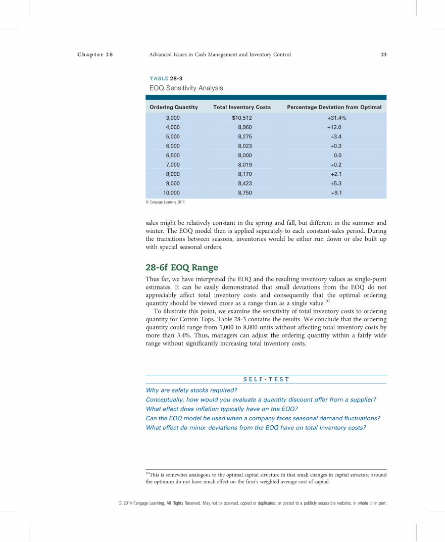
To illustrate this point, we examine the sensitivity of total inventory costs to orderingquantity for Cotton Tops. Table 28-3 contains the results. We conclude that the orderingquantity could range from 5,000 to 8,000 units without affecting total inventory costs bymore than 3.4%. Thus, managers can adjust the ordering quantity within a fairly widerange without significantly increasing total inventory costs.

S E L F - T E S T

Why are safety stocks required?

Conceptually, how would you evaluate a quantity discount offer from a supplier?

What effect does inflation typically have on the EOQ?

Can the EOQ model be used when a company faces seasonal demand fluctuations?

What effect do minor deviations from the EOQ have on total inventory costs?

TABLE 28-3

EOQ Sensitivity Analysis

Ordering Quantity Total Inventory Costs Percentage Deviation from Optimal

3,000 $10,512 +31.4%

4,000 8,960 +12.0

5,000 8,275 +3.4

6,000 8,023 +0.3

6,500 8,000 0.0

7,000 8,019 +0.2

8,000 8,170 +2.1

9,000 8,423 +5.3

10,000 8,750 +9.1


10This is somewhat analogous to the optimal capital structure in that small changes in capital structure aroundthe optimum do not have much effect on the firm’s weighted average cost of capital.



S U M M A R Y

This chapter discussed the goals of cash management and how a company mightdetermine its optimal cash balance using the Baumol model. It also discussed how anoptimal inventory policy might be identified using the Economic Ordering Quantity(EOQ) model. The key concepts covered are listed below.

• A policy that strives for zero working capital not only generates cash but also speedsup production and helps businesses operate more efficiently. This concept has itsown definition of working capital: Inventories + Receivables − Payables. Therationale is that inventories and receivables are the keys to making sales and thatinventories can be financed by suppliers through accounts payable.

• The primary goal of cash management is to minimize the amount of cash a firmholds while maintaining a sufficient target cash balance to conduct business.

• The Baumol model provides insights into the optimal cash balance. The modelbalances the opportunity cost of holding cash against the transaction costs associatedwith obtaining cash either by selling marketable securities or by borrowing:

Optimal cash infusion ¼ffiffiffiffiffiffiffiffiffiffiffiffiffiffiffiffiffi2 Fð Þ Tð Þ

r

r

• Firms generally set their target cash balances at the level that holds the risk ofrunning out of cash to some acceptable level. Monte Carlo simulation can be helpfulin setting the target cash balance.

• Firms use inventory control systems such as the red-line method, the two-binmethod, and computerized inventory control systems to help them keep track ofactual inventory levels and to ensure that inventory levels are adjusted as saleschange. Just-in-time (JIT) systems are used to hold down inventory costs and,simultaneously, to improve the production process. Outsourcing is the practice ofpurchasing components rather than making them in-house.

• Inventory can be accounted for in four different ways: (1) specific identification,(2) first-in, first-out (FIFO), (3) last-in, first-out (LIFO), and (4) weightedaverage.

• Inventory costs can be divided into three parts: carrying costs, ordering costs, andstock-out costs. In general, carrying costs increase as the level of inventory rises, butordering costs and stock-out costs decline with larger inventory holdings.

• Total carrying cost (TCC) is equal to the percentage cost of carrying inventory (C)multiplied by the purchase price per unit of inventory (P) times the average numberof units held (A): TCC = (C)(P)(A).

• Total ordering cost (TOC) is equal to the fixed cost of placing an order (F)multiplied by the number of orders placed per year (N): TOC = (F)(N).

• Total inventory costs (TIC) equal total carrying cost (TCC) plus total ordering cost(TOC): TIC = TCC + TOC.

• The Economic Ordering Quantity (EOQ) model is a formula for determining theorder quantity that will minimize total inventory costs:

EOQ ¼ffiffiffiffiffiffiffiffiffiffiffiffiffiffiffiffiffi2 Fð Þ Sð ÞCð Þ Pð Þ

s

Here F is the fixed cost per order, S is annual sales in units, C is the percentage cost ofcarrying inventory, and P is the purchase price per unit.



• The order point is the inventory level at which new items must be ordered.• Safety stocks are held to avoid shortages, which can occur if (1) sales increase by

more than expected or (2) shipping delays are encountered on inventory ordered.The cost of carrying a safety stock, which is separate from that based on the EOQmodel, is equal to the percentage cost of carrying inventory multiplied by thepurchase price per unit times the number of units held as the safety stock.

Q U E S T I O N S

(28-1) Define each of the following terms:

a. Baumol modelb. Total carrying cost; total ordering cost; total inventory costsc. Economic Ordering Quantity (EOQ); EOQ model; EOQ ranged. Reorder point; safety stocke. Red-line method; two-bin method; computerized inventory control systemf. Just-in-time system; outsourcing

(28-2) Indicate by a (+), (−), or (0) whether each of the following events would probably causeaverage annual inventory holdings to rise, fall, or be affected in an indeterminate manner:

a. Our suppliers change from delivering by train to air freight. __________________b. We change from producing just-in-time to meet seasonal

demand to steady, year-round production. __________________c. Competition in the markets in which we sell increases. __________________d. The general rate of inflation rises. __________________e. Interest rates rise; other things are constant. __________________

(28-3) Assuming the firm’s sales volume remained constant, would you expect it to have a highercash balance during a tight-money period or during an easy-money period? Why?

(28-4) Explain how each of the following factors would probably affect a firm’s target cashbalance if all other factors were held constant.

a. The firm institutes a new billing procedure that better synchronizes its cash inflowsand outflows.

b. The firm develops a new sales forecasting technique that improves its forecasts.c. The firm reduces its portfolio of U.S. Treasury bills.d. The firm arranges to use an overdraft system for its checking account.e. The firm borrows a large amount of money from its bank and also begins to write far

more checks than it did in the past.f. Interest rates on Treasury bills rise from 5% to 10%.

P R O B L E M S

(28-1) The Gentry Garden Center sells 90,000 bags of lawn fertilizer annually. The optimal safetystock (which is on hand initially) is 1,000 bags. Each bag costs the firm $1.50, inventorycarrying costs are 20%, and the cost of placing an order with its supplier is $15.

a. What is the Economic Ordering Quantity?b. What is the maximum inventory of fertilizer?c. What will be the firm’s average inventory?d. How often must the company order?

IntermediateProblems 1–2

Economic OrderingQuantity



(28-2) Barenbaum Industries projects that cash outlays of $4.5 million will occur uniformlythroughout the year. Barenbaum plans to meet its cash requirements by periodicallyselling marketable securities from its portfolio. The firm’s marketable securitiesare invested to earn 12%, and the cost per transaction of converting securities tocash is $27.

a. Use the Baumol model to determine the optimal transaction size for transfers frommarketable securities to cash.

b. What will be Barenbaum’s average cash balance?c. How many transfers per year will be required?d. What will be Barenbaum’s total annual cost of maintaining cash balances? What

would the total cost be if the company maintained an average cash balance of $50,000or of $0 (it deposits funds daily to meet cash requirements)?

S P R E A D S H E E T P R O B L E M

(28-3) Start with the partial model in the file Ch28 P03 Build a Model.xls on the textbook’s Website. The following inventory data have been established for the Adler Corporation.

(1) Orders must be placed in multiples of 100 units.(2) Annual sales are 338,000 units.(3) The purchase price per unit is $3.(4) Carrying cost is 20% of the purchase price of goods.(5) Cost per order placed is $24.(6) Desired safety stock is 14,000 units; this amount is on hand initially.(7) Two weeks are required for delivery.

a. What is the EOQ?b. How many orders should the firm place each year?c. At what inventory level should a reorder be made? Hint: Reorder point = (Safety stock

+ Weeks to deliver × Weekly usage) − Goods in transit.d. Calculate the total costs of ordering and carrying inventories if the order quantity is

(1) 4,000 units, (2) 4,800 units, or (3) 6,000 units. What are the total costs if the orderquantity is the EOQ?

e. What are the EOQ and total inventory costs if the following were to occur?

(1) Sales increase to 500,000 units.(2) Fixed order costs increase to $30; sales remain at 338,000 units.(3) Purchase price increases to $4; sales and fixed costs remain at original values.

M I N I C A S E

Andria Mullins, financial manager of Webster Electronics, has been asked by the firm’sCEO, Fred Weygandt, to evaluate the company’s inventory control techniques and to leada discussion of the subject with the senior executives. Andria plans to use as an exampleone of Webster’s “big ticket” items, a customized computer microchip that the firm usesin its laptop computers. Each chip costs Webster $200, and it must also pay its supplier a$1,000 setup fee on each order; the minimum order size is 250 units. Webster’s annualusage forecast is 5,000 units, and the annual carrying cost of this item is estimated to be20% of the average inventory value.

Andria plans to begin her session with the senior executives by reviewing some basicinventory concepts, after which she will apply the EOQ model to Webster’s microchip

Optimal CashTransfer

Build a Model:Inventory

Management

r e s o u r c e



inventory. As her assistant, you have been asked to help her by answering the followingquestions:

a. Why is inventory management vital to the financial health of most firms?b. What assumptions underlie the EOQ model?c. Write out the formula for the total costs of carrying and ordering inventory, and then

use the formula to derive the EOQ model.d. What is the EOQ for custom microchips? What are total inventory costs if the EOQ

is ordered?e. What is Webster’s added cost if it orders 400 units at a time rather than the EOQ

quantity? What if it orders 600 units?f. Suppose it takes 2 weeks for Webster’s supplier to set up production, make and test

the chips, and deliver them to Webster’s plant. Assuming certainty in delivery timesand usage, at what inventory level should Webster reorder? (Assume a 52-week year,and assume Webster orders the EOQ amount.)

g. Of course, there is uncertainty in Webster’s usage rate as well as in delivery times, sothe company must carry a safety stock to avoid running out of chips and having tohalt production. If a 200-unit safety stock is carried, what effect would this have ontotal inventory costs? What is the new reorder point? What protection does the safetystock provide if usage increases or if delivery is delayed?

h. Now suppose Webster’s supplier offers a discount of 1% on orders of 1,000 or more.Should Webster take the discount? Why or why not?

i. For many firms, inventory usage is not uniform throughout the year but instead followssome seasonal pattern. Can the EOQ model be used in this situation? If so, how?

j. How would these factors affect an EOQ analysis?(1) The use of just-in-time procedures.(2) The use of air freight for deliveries.(3) The use of a computerized inventory control system, in which an electronic

system automatically reduced the inventory account as units were removedfrom stock and, when the order point was hit, automatically sent an electronicmessage to the supplier placing an order. The electronic system would ensurethat inventory records are accurate and that orders are placed promptly.

(4) The manufacturing plant is redesigned and automated. Computerized processequipment and state-of-the-art robotics are installed, making the plant highlyflexible in the sense that the company can quickly switch from the production ofone item to another at a minimum cost. This makes short production runs morefeasible than under the old plant setup.

k. Webster runs a $100,000 per month cash deficit, requiring periodic transfers from itsportfolio of marketable securities. Broker fees are $32 per transaction, and Websterearns 7% on its investment portfolio. How can Andria use the EOQ model todetermine how Webster should liquidate part of its portfolio to provide cash?

S E L E C T E D A D D I T I O N A L C A S E S

The following cases from CengageCompose cover many of the concepts discussed in thischapter and are available at compose.cengage.com.

Klein-Brigham Series:Case 33, “Upscale Toddlers, Inc.”; Case 79, “Mitchell Lumber Co.”; Case 34, “Texas RoseCompany”; and Case 67, “Bridgewater Pool Company,” all of which focus on receivablesmanagement.



Documents

CHAPTER Advanced Issues in Cash Management …...CHAPTER28 Advanced Issues in Cash Management and Inventory Control T his chapter provides detailed coverage of several working capital