CHAPTER 9

THE CONTINUOUS AND FINITE ELEMENT TRANSVERSE VIBRATION

ANALYSES OF SIMPLE ROTOR SYSTEMS

In the previous chapter, we studied transverse vibrations of multi-DOF rotor systems by considering

the shaft as massless and flexible by using the direct and transfer matrix methods. While dealing with

torsional vibrations, we encountered rotors that could be modelled accurately, if one models them as a

continuous system. In the present chapter, the shaft will be considered as having the distributed mass

and stiffness properties. Equations of motion are obtained by using the Hamilton’s principle. For

simple boundary conditions, the closed form solutions are obtained by the method of separation of

variables. However, for more complex boundary conditions continuous system approach becomes

impracticable. Hence, we need to resort for some approximate methods, e.g., the finite element

method. For the finite element analysis of rotor systems, the Euler-Bernoulli beam model is initially

considered for development of the elemental mass and stiffness matrices. Both the free and forced

vibration analysis using the finite element method is illustrated for a variety of conditions at supports.

In the finite element method, the overall size of matrices increases with the number of degrees of

freedom of the system. Quite often it is required to reduce the size of actual matrices to be solved to

save the computational time. To handle such cases, the static and dynamic reductions (or

condensations) are described. These reductions do introduce some of amount of approximation in

solutions. In subsequent chapters, higher order effects like the rotary inertia, shear deformation, and

gyroscopic moment effects would be considered for the analysis by using the finite element method.

9.1 Governing Equations in Continuous Systems

In the present section one-dimensional governing equations with boundary conditions (i.e., the

boundary value problem) of a shaft will be formulated for transverse vibrations by using the

Hamilton’s principle. This principle requires various energies, e.g. the strain and kinetic energies, and

the work done by external forces. Consider a circular beam of length, L, and the cross sectional area

of the beam is A, as shown in Figure 9.1. It is acted upon by an external distributed force, f(z, t), over

a length of the shaft as well as a concentrated force, f0(t), at z = z0 acting in the direction of y-axis.

Thus, the beam is subjected to lateral (the transverse or the bending) vibrations in the vertical

direction. For the Euler-Bernoulli beam the motion in the vertical and horizontal planes are

uncoupled, i.e. the vertical force would produce only vertical displacements (the linear as well as the

angular) and similarly the horizontal force would produce only horizontal displacements. Hence, the

analysis in the two orthogonal planes could be done separately, and it would be remaining the

506

identical. The analysis presented here is for the vertical plane y-z and the analysis in the horizontal

plane z-x will be remaining same.

Let us consider cross-sectional plane at a distance, z, as shown in Fig. 9.2. According to the Euler-

Bernoulli beam theory a plane cross section before the bending remains plane even after the bending.

Thus, the plane has a rotation about x-axis and is given by a slope, x

v

zϕ

∂= −

∂, of the elastic curve

(i.e., the neutral axis) as shown in Figure 9.2. Let v be the transverse displacement in the y-direction of

the neutral axis at the distance, z. Thus, all the points of the chosen plane would have the same

transverse displacement. Let us choose a point P, with (x, y, z) as its co-ordinates in the chosen plane

at a distance, z. Thus to define the position of the chosen plane two displacement variables are: v and

xϕ .

Figure 9.1 An Euler-Bernoulli beam before the bending

Figure 9.2 The elastic line of the beam after the bending

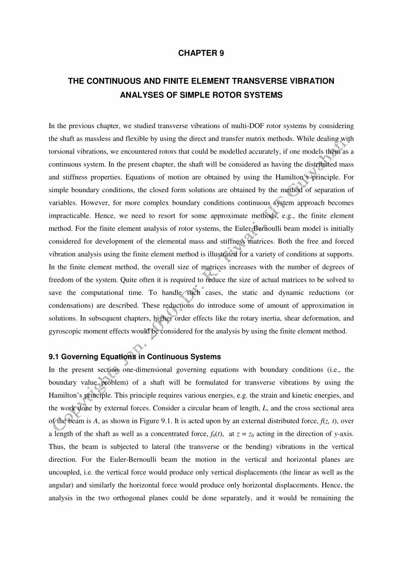
Thus the displacement field of the point P, under the assumption of small displacements, can be

obtained as (see Figure 9.3)

507

0xu = ; ( , )y

u v z t= ; ( , )

z x

v z tu y y yv

zϕ

∂′= = − = −

∂ (9.1)

with

x

v

zϕ

∂= −

∂ (9.2)

where u is the displacement component of the point P, and subscripts (i.e., x, y, z) represent the

directions. The prime ( ′ ) represents the derivative with respect to the spatial coordinate, z.

Figure 9.3 The displacement field of the point P under bending of the shaft

Corresponding the strain and stress fields are

( , )zzz

uyv z t

zε

∂′′= =

∂; ( )

1 10

2 2

y z

yz

u uv v

z yε

∂ ∂′ ′= + = − =

∂ ∂ ; 0xx yy xy yz zxε ε ε ε ε= = = = =

(9.3)

and

( , )zz Eyv z tσ ′′= ; 0xx yy xy yz zx

σ σ τ τ τ= = = = = (9.4)

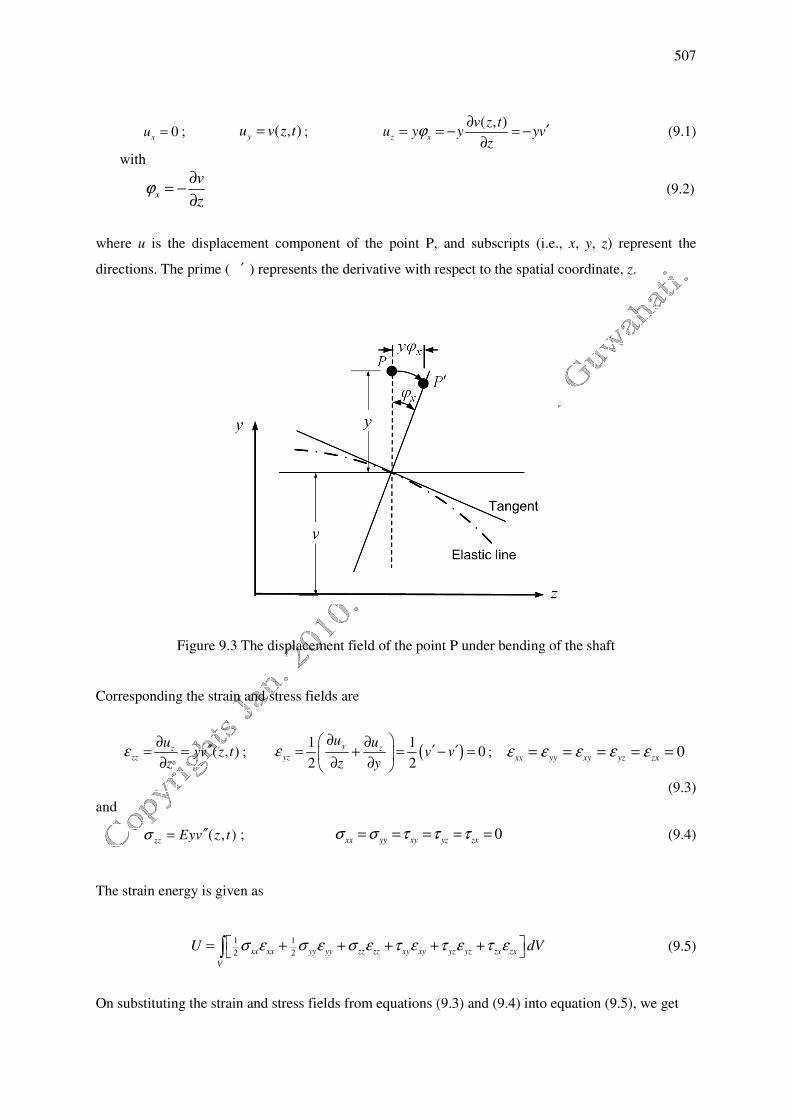
The strain energy is given as

1 1

2 2xx xx yy yy zz zz xy xy yz yz zx zx

V

U dVσ ε σ ε σ ε τ ε τ ε τ ε = + + + + + ∫ (9.5)

On substituting the strain and stress fields from equations (9.3) and (9.4) into equation (9.5), we get

508

{ }21 1 12 2 2 2

2 2 2

0 0 0

1( , )

2

L L L

zz zz xxV

A A

U dV Ey v dAdz E y dA v dz EI v z t dzσ ε

′′ ′′ ′′= = = =

∫ ∫ ∫ ∫ ∫ ∫ (9.6)

with

2

xx

A

I y dA= ∫

where xxI is the moment of inertia of the cross section of the beam about the axis of bending, i.e.

about the x-axis.

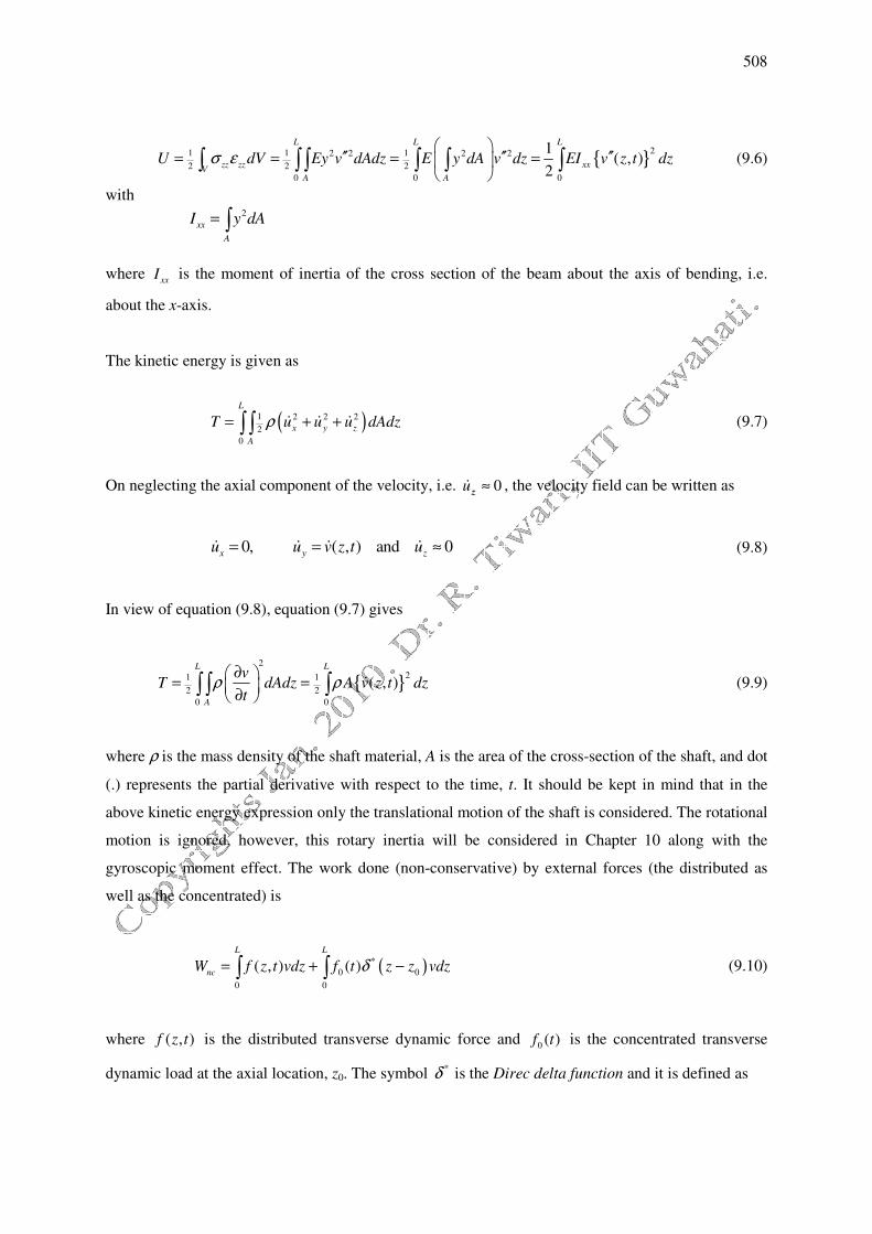
The kinetic energy is given as

( )1 2 2 2

2

0

L

x y z

A

T u u u dAdzρ= + +∫ ∫ � � � (9.7)

On neglecting the axial component of the velocity, i.e. 0zzu ≈� , the velocity field can be written as

0, ( , ) and 0x y z

u u v z t u= = ≈� � � � (9.8)

In view of equation (9.8), equation (9.7) gives

{ }2

21 1

2 2

0 0

( , )

L L

A

vT dAdz A v z t dz

tρ ρ

∂ = =

∂ ∫ ∫ ∫ � (9.9)

where ρ is the mass density of the shaft material, A is the area of the cross-section of the shaft, and dot

(.) represents the partial derivative with respect to the time, t. It should be kept in mind that in the

above kinetic energy expression only the translational motion of the shaft is considered. The rotational

motion is ignored, however, this rotary inertia will be considered in Chapter 10 along with the

gyroscopic moment effect. The work done (non-conservative) by external forces (the distributed as

well as the concentrated) is

( )*

0 0

0 0

( , ) ( )

L L

ncW f z t vdz f t z z vdzδ= + −∫ ∫ (9.10)

where ( , )f z t is the distributed transverse dynamic force and 0 ( )f t is the concentrated transverse

dynamic load at the axial location, z0. The symbol *δ is the Direc delta function and it is defined as

509

0

* *

0 0 0( ) 1 for , and ( ) 0 otherwisez z z z z zδ δ− = = − = (9.11)

and it has the following property

*

0 0( ) ( ) ( )g z z z dz g zδ

∞

−∞− =∫ (9.12)

In equation (9.10) by use of the Direc delta function, it enables to represent the point (or the

concentrated) dynamic force as a distributed force description in the form of an integral.

The Hamilton’s principle for a conservative dynamical system states that the variation of the integral

of the Lagrangian function ( )L T U= − taken over a given interval of time is a stationary (refer

Chapter 7 for more details). Hence, the element equation of motion and boundary conditions can be

obtained as

( )2

1

0

t

nc

t

T U W dtδ δ − + = ∫ (9.13)

where the above form is called the extended Hamilton’s principle, which is valid for the non-

conservative dynamical systems also. On substituting equations (9.6), (9.9) and (9.10) into equation

(9.13), we get

22 2

*0 0

2

1

21 1

2 20

( , ) ( , ) ( , ) ( ) ( ) 0

t L

xx

t

v z t v z tA EI f z t v f t z z v dzdt

ztδ ρ δ

∂ ∂− + + − =∂∂

∫ ∫ (9.14)

On taking the variational operator inside the integral of the above equation, we get

2

1

2 2*

0 02 2

0

( , ) ( , ) ( , ) ( , )( , )( ) ( ) ( )( ) 0

t L

xx

t

v z t v z t v z t v z tA EI f z t v f t z z v dzdt

t t z zρ δ δ δ δ δ ∂ ∂ ∂ ∂

− + + − = ∂ ∂ ∂ ∂

∫ ∫

For obtaining the weak formulation of the above equation, on integrating by parts of the first two

terms, respectively, with respect to t and z, we get

2 2

11

2

2

0

( , ) ( , )( , ) ( , )

t tL

tt

v z t v z tA v z t A v z t dt dz

t tρ δ ρ δ ∂ ∂

− ∂ ∂

∫ ∫

510

+2

1

2 2 2 2

2 2 2 2

00 0

( , ) ( , ) ( , ) ( , )( , ) ( , )

L Lt L

xx xx xx

t

v z t v z t v z t v z tEI EI v z t EI v z t dz dt

z z z z z zδ δ δ

∂ ∂ ∂ ∂ ∂ ∂ − + −

∂ ∂ ∂ ∂ ∂ ∂ ∫ ∫

{ }2

1

*

0 0

0

( , ) ( ) ( ) 0

t L

t

f z t f t z z vdzdtδ δ+ + − =∫ ∫ (9.15)

The variation of the displacement, v, at two instances t1 and t2 is zero; hence, the first term is zero. On

rearranging terms in equation (9.15), we get

2

1

2 2 2 2 2*

0 02 2 2 2 2

0 0 0

( ) 0

LLt L

xx xx xx

t

v v v v vEI A f f z z vdz EI EI v dt

z z t z z z zρ δ δ δ δ

∂ ∂ ∂ ∂ ∂ ∂ ∂ + − − − + − = ∂ ∂ ∂ ∂ ∂ ∂ ∂

∫ ∫

(9.16)

Since vδ is the variation of displacement which is chosen arbitrary, hence we will have the

differential equation of motion from the coefficient of vδ within the double integral of the above, as

*

0 0( , ) ( , ) ( , ) ( ) ( )xxEI v z t Av z t f z t f t z zρ δ′′′′ + = + −�� (9.17)

Similarly, last two terms in equation (9.16) should be individually equated to zero to get boundary

conditions as

0( , ) ( , ) 0

L

xxEI v z t v z tδ′′ ′ = and 0

( , ) ( , ) 0L

xxEI v z t v z tδ′′′ = (9.18)

Equations (9.17) and (9.18) form a boundary value problem. It should be noted that equation (9.17) is

a linear partial differential equation. The types of the independent variables are the spatial, z, and the

temporal, t, in nature. The governing equation can be solved both for the free and forced vibrations in

the closed form for simple boundary conditions, e.g., the simply supported, free-free, fixed-free, and

fixed-fixed support conditions.

Table 9.1 State variables for different boundary conditions

S.N. Boundary conditions xxEI v′′ v′

xxEI v′′′ v

1 Simply supported 0 - - 0

2 Freely supported 0 - 0 -

3 Fixed supported - 0 - 0

511

It should be noted that terms xxEI v′′ and

xxEI v′′′ represent the bending moment and the shear force,

respectively; whereas v′ and v are the transverse angular and linear displacements, respectively. Table

9.1 summaries for which support conditions these state variables become zero. It can be observed that

the bending moment and the transverse angular displacement are never zero simultaneously; similarly,

the shear force and the transverse linear displacement are never zero simultaneously. For the free

vibration analysis purpose the closed form solution procedures have been presented in subsequent

section for few cases.

9.2 Natural Frequencies and Mode Shapes

Natural frequencies and mode shapes in the closed form are obtained by considering the

homogeneous equation (for the free vibration) of the beam governing equation (9.17). We consider

the undamped bending vibrations of the shaft with the uniform sectional property. For the free

vibration, letting external force f(z, t) = f0 = 0. On assuming the free response as a simple harmonic,

we have assumed the free response of the following from

( , ) ( ) ( )v z t z tχ η= so that ( , ) ( ) ( )v z t z tχ η′′′′ ′′′′= and ( , ) ( ) ( )v z t z tχ η= ���� (9.19)

where χ(z) is the eigen function (i.e., the mode shape), and for the free vibration the function, ( )tη ,

has the following form

( ) cos sinnf nf

t A t B tη ω ω= + so that 2( ) ( )nft tη ω η= −�� (9.20)

in which and ωnf is the natural frequency, and A and B are integral constants to be determined from

initial conditions of the problem. On substituting (9.19) and (9.20) in equation (9.17), we get

44

4

( )( ) 0

d zz

dz

χβ χ− = (9.21)

with 2

4 nf

xx

A

EI

ρ ωβ = (9.22)

The general solution of equation (9.21) is

1 2 3 4( ) sin cos sinh coshz C z C z C z C zχ β β β β= + + + (9.23)

where C1, C2, C3 and C4 are integration constants to be evaluated from boundary conditions.

512

Let us consider the shaft with the simply supported end conditions. Boundary conditions at shaft ends

imply following conditions on the eigen function

(0) ( ) 0Lχ χ= = and (0) ( ) 0Lχ χ′′ ′′= = (9.24)

On taking derivative of equation (9.23) twice with respect to z, we get

2 2 2 2

1 2 3 4( ) sin cos sinh coshz C z C z C z C zχ β β β β β β β β′′ = − − + + (9.25)

On application of four boundary conditions of (9.24), in equations (9.23) and (9.25), we get

1

2

2 2

3

2 2 2 2

4

0 1 0 1 0

sin cos sinh cosh 0

0 0 0

sin cos sinh cosh 0

C

CL L L L

C

CL L L L

β β β β

β β

β β β β β β β β

=

− − −

(9.26)

From the first and third set of equations in the matrix equation (9.26) (i.e., C2 + C4 = 0 and C2 - C4 =

0), we get C2 = C4 = 0. Hence, finally equation (9.26) reduces to (after elimination of the first and

third rows, and the second and fourth columns)

1

2 2

3

sin sinh 0

sin sinh 0

CL L

CL l

β β

β β β β

= −

(9.27)

On taking determinant of homogeneous matrix equation (9.27), it gives

sin sinh 0L Lβ β β = (9.28)

In the above equation all three terms have a common solution, i.e. β = 0. The first and third terms (i.e.,

β and sinhβL) have no other solution, however, the second term (i.e., sinhβL) has infinite number

solutions. Excluding the trivial solution (i.e. β ≠ 0 that means sin sinh 0L Lβ β= ≠ ), we obtain the

frequency equation as

sin 0Lβ = for β ≠ 0 (9.29)

513

which will be satisfied for

nL nβ π= ; n = 1, 2, … (9.30)

In view of equation (9.30), from equation (9.22) the natural frequency in nth mode is

2

4( )

n

xx

nf

EIn

ALω π

ρ= (9.31)

Hence we have an interesting relation between the fundamental mode and higher modes, i.e.

1

2

nnf nfnω ω= .

Now to get the mode shape, from the first set of equation (9.27), we have

1 3sin sinh 0C L C Lβ β+ = (9.32)

Since we have sinh 0Lβ ≠ when 0Lβ ≠ , hence C3 = 0. However, sin 0Lβ = even for 0Lβ ≠ , hence

C1 ≠ 0. Since now we have C2 = C3 = C4 = 0, and in view of equation (9.31), from equation (9.23) we

have

1 1( ) sin sinn

nz C z C z

L

πχ β= = (9.33)

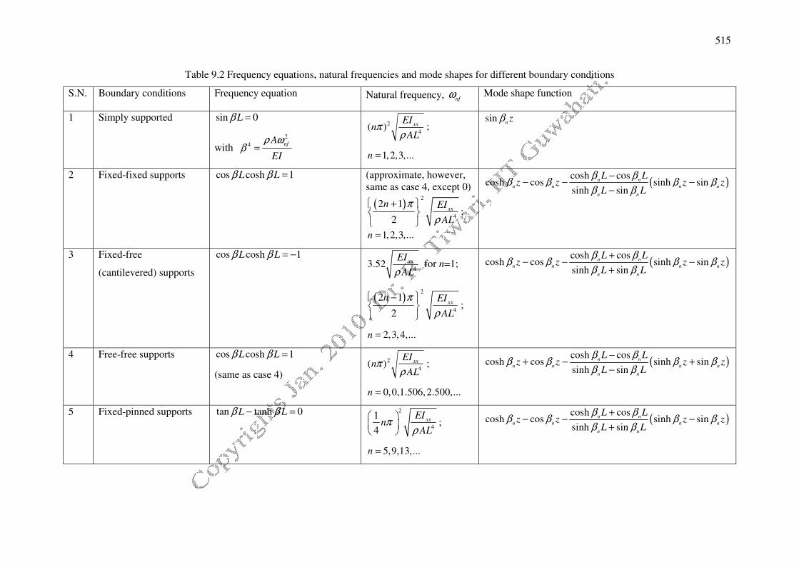
The procedure is same for the shaft with other boundary conditions. Frequency equations and natural

frequencies for the fixed-fixed, fixed-free, free-free, and fixed-pinned shaft boundary conditions are

given in Table 9.2. It should be noted that the frequency equation for the fixed-fixed and free-free

boundary conditions are the same. For free-free boundary conditions, two ‘zero’ frequencies are

corresponding to the translational and rotational rigid body modes, respectively. In these rigid body

modes, in the former case the beam would have rigid body up and down motion whereas in the latter

case the beam would have rigid body rotation about the centre of gravity. For the fixed-fixed case,

two ‘zero’ frequencies are corresponding to the translational and rotational rigid body modes and are

not feasible. This is due to the boundary condition that we need to satisfy while solving the

differential equation. For the fixed-fixed case, both the end must have zero translational and rotational

displacements, and for the rigid body motion all the particle of the beam should have the same

displacements (either translational or rotational). So the rigid body modes are only possible with zero

translational and zero rotational displacements, that means corresponding to two zero natural

514

frequencies from the frequency equations only motion possible is that of zero displacements i.e. no

motion at all. Hence, these zero natural frequency has no practical significance for fixed-fixed

boundary conditions of the beam. This could be proved by directly solving differential equation with

zero natural frequencies subject to boundary conditions of the fixed-fixed case and it is left to the

reader as an excise.

515

Table 9.2 Frequency equations, natural frequencies and mode shapes for different boundary conditions

S.N. Boundary conditions Frequency equation Natural frequency, nfω Mode shape function

1 Simply supported sin 0Lβ =

with

2

4 nfA

EI

ρ ωβ =

2

4( ) xxEIn

ALπ

ρ;

1,2,3,...n =

sinnzβ

2 Fixed-fixed supports cos cosh 1L Lβ β = (approximate, however,

same as case 4, except 0)

( )2

4

2 1

2

xxn EI

AL

π

ρ

+

;

1,2,3,...n =

( )cosh cos

cosh cos sinh sinsinh sin

n n

n n n n

n n

L Lz z z z

L L

β ββ β β β

β β

−− − −

−

3 Fixed-free

(cantilevered) supports

cos cosh 1L Lβ β = −

43.52 xxEI

ALρ for n=1;

( )2

4

2 1

2

xxn EI

AL

π

ρ

−

;

2,3,4,...n =

( )cosh cos

cosh cos sinh sinsinh sin

n n

n n n n

n n

L Lz z z z

L L

β ββ β β β

β β

+− − −

+

4 Free-free supports cos cosh 1L Lβ β =

(same as case 4)

2

4( ) xxEIn

ALπ

ρ;

0,0,1.506,2.500,...n =

( )cosh cos

cosh cos sinh sinsinh sin

n n

n n n n

n n

L Lz z z z

L L

β ββ β β β

β β

−+ − +

−

5 Fixed-pinned supports tan tanh 0L Lβ β− = 2

4

1

4

xxEI

nAL

πρ

;

5,9,13,...n =

( )cosh cos

cosh cos sinh sinsinh sin

n n

n n n n

n n

L Lz z z z

L L

β ββ β β β

β β

+− − −

+

516

Orthogonality conditions

The most important properties of normal modes are that of the orthogonality. It is this property that

makes possible the uncoupling of equations of motion in different mode of vibrations. For two

different frequencies m nω ω≠ , normal modes must satisfy

0

( ) ( ) 0

L

m nA z z dzρ χ χ =∫ for m n≠ (9.34)

For m = n

2

0

( )

L

m mA z dz Mρ χ =∫ (9.35)

in which Mm is called the “generalized mass” in the mth mode. On the similar lines, we have

0

( ) ( ) 0

L

xx m nEI z z dzχ χ′′ ′′ =∫ for m n≠ (9.36)

For m = n

2

0

( )

L

xx m mEI z dz Kχ ′′ =∫ (9.37)

in which Km is called the “generalized stiffness” in the mth mode. These properties would be useful for

the modal analysis in forced vibrations.

9.3 Forced Vibrations

The orthogonality property now will be used to obtain uncoupled equations of motion for the

continuous system, which is easier to handle. Having obtained natural frequencies and mode shapes,

the transverse displacement of the shaft for forced vibrations can be written as

1

( , ) ( ) ( )i i

i

v z t z tχ η∞

=

=∑ (9.38)

in which ηi(t) is the generalized coordinate. Theoretically, infinite numbers of modes for continuous

systems are possible. However, contribution of higher modes towards the response is negligible.

Hence in computation only first few modes are considered. Substituting equation (9.38) in equation

517

(9.17), multiplying both sides by kχ , integrating in the domain of the shaft and applying orthogonality

condition of normal modes, the partial differential equation of motion can be discretized into

uncoupled ordinary differential equations of motion as

2( ) ( ) ( )

ii nf i it t f tη ω η+ =�� i = 1, 2, … (9.39)

with

/inf i i

K Mω =

where inf

ω is the ith natural frequency, and fi is the generalized force in the i

th mode and is given as

0

1( ) ( , ) ( )

L

i i

i

f t f z t z dzM

χ= ∫ (9.40)

The solution of equation (9.39) can be obtained by the Duhamel’s or convolution integral

(Meirovitch, 1986) as

0

(0)1( ) ( )sin ( ) (0)cos sin

i i i

i i

t

ii i nf i nf nf

nf nf

t f t d t tη

η τ ω τ τ η ω ωω ω

= − + +∫�

(9.41)

where ηi(0) and ( )i tη� are initial conditions and τ is a dummy variable.

For example, consider a simply supported shaft with a uniform cross section subjected to a sinusoidal

force, 0 sinF tω , applied to a section z0 = 0.5L i.e. at the mid span. From equation (9.40) the

generalized force is given by

* ( 1) / 2

0 0 0

0

1 1 1( ) ( 0.5 ) sin sin sin sin ( 1) sin

2

L

i

i

i i i

i z if t z L F t dz F t F t

M L M M

π πδ ω ω ω−

= − = = −

∫ ,

1,3,5,...i = (9.42)

The generalised mass from equation (9.35) is given as

2

0

sin2

L

i

i z ALM A dz

L

π ρρ

= =

∫ (9.43)

518

In view of equation (9.43), equation (9.42) gives

( 1) / 2 02

( ) ( 1) sini

i

Ff t t

ALω

ρ−= − , 1,3,5,...i = (9.44)

For the zero initial displacement and velocity, the response from equation (9.41) can be written as

( 1) / 2 ( 1) / 20 0

2

0

sin sin2 21 1

( ) ( 1) sin sin ( ) ( 1)

1

i

i

i

i i

i

i

nftnfi i

i nf

nf nf

nf

nf

t tF F

t t t dAL AL

ωω ω

ωη ω ω τ τ

ρ ω ρ ω ωω

ω

− −

−

= − − = −

−

∫

1,3,5,...i = (9.45)

The steady state transverse displacement of the beam from equation (9.38), in view of equation (9.45)

can be written as (dropping second term within the bracket (i.e. sininftω ) which corresponds to the

transient part, and in actual case it dies out after some time in the presence of damping)

( )

( ){ }( 1) / 20

221 1,3,5,...

sin /2( , ) ( ) ( ) ( 1) sin

1 /i i

i

i i

i inf nf

i z LFv z t z t t

AL

πχ η ω

ρ ω ω ω

∞ ∞−

= =

= = − −

∑ ∑ (9.46)

It is apparent that all even modes do not contribute to the steady state forced response. It is also of

interest to compare the contribution of various modes. This comparison can be done on the basis of

maximum modal displacement disregarding the manner in which these displacements combine. The

amplitude will indicate the relative importance of the modes. Furthermore, for all modes (except even

modes), the modal contribution is simply in proportion to 21/

infω . Therefore in higher modes the factor

21/

infω becomes smaller, and hence its contribution can be ignored in the superimposition of modes.

The above analysis based on the continuous approach becomes impractical for real rotor systems

because of complex boundary conditions. For such cases the finite element method is quite versatile

and practical. However, the closed form solution for simple cases could be used for checking and

performing the convergence study for the computer code developed based on the finite element

method, and subsequently the developed code could be used for complex problems.

519

9.4 A Brief Review on Application of FEM in Rotor-Bearing Systems

In the past several decades various methods have been developed to analyze the dynamic behaviour of

rotor bearing systems, e.g., the influence coefficient, transfer matrix, dynamic stiffness, mechanical

impedance, finite element methods, etc. Of several methods the finite element method (FEM) is one,

which is particularly well suited for modelling the large scale and complex rotor-bearing-foundation

systems. As compared to the torsional and axial vibrations, initially researchers attempted more

complex transverse vibration analyses of rotor-bearing systems.

The Euler-Bernoulli beam accounts for the major effects of bending in beams, which is due to the

pure bending. In this theory, any plane cross-section of the beam before bending is assumed to remain

plane after bending, and remain normal to the elastic (neutral) axis. Therefore, a beam cross section

has not only the translation but also the rotation. Rayleigh accounts for the energy arising out of this

cross-sectional rotation, which he called the rotary inertia. Subsequently, Timoshenko accounted for

the shear strain energy in the beam due to the bending caused by the shear force. The Timoshenko

beam usually refers to a beam in which both the rotary inertia and shear deformation effects are taken

into account. The effects of rotary inertia and shear deformation are predominant in the transverse

vibration of the beam having large cross-section (i.e., for thick beams; for a circular shaft we have the

condition for thicki beam as / .r L > 0 1 where r is the radius of gyration of the shaft and L is the

length of the shaft). If Timoshenko beams spins also, then gyroscopic effects also have an important

role along with the rotary inertia and shear effects.

Historically, Ruhl (1970), and Ruhl and Booker (1972) were amongst the first researchers to utilize

the finite element method to study the stability and the unbalance response of turbo-rotor systems. In

their finite element formulations, only the elastic bending and translational kinetic energies were

included. However, many effects such as the rotary inertia, shear deformations, gyroscopic moments,

and the internal and external damping were all neglected in their finite element analysis. These higher

order effects can be a very important for some configurations, as discussed in books by Dimentberg

(1961) and Tondl (1965). McVaugh and Nelson (1976) generalized Ruhl’s work by utilizing the

Rayleigh beam model to devise a finite element formulation including the effects of rotary inertia,

gyroscopic moments and axial load to simulate a flexible rotor system supported on the linear

stiffness and (viscous) damping bearings. In order to facilitate the computations of natural whirl

frequencies and unbalance responses, element equations were transformed into a rotating frame of

reference for the case of isotropic bearings (i.e., cross-coupled coefficients are equal and direct

coefficients are equal for both the stiffness and the damping). Also to save the computational time the

Guyan (static) reduction procedure (1965) was adopted to reduce the size of system matrices. Zorzi

and Nelson (1977) extended the work of McVaugh and Nelson by the inclusion of both internal

520

viscous and hysteretic damping in the same finite element model. At about same time, Rouch and Kao

(1979), and Nelson (1980) utilized the Timoshenko beam theory for establishing shape functions.

Based on these shape functions the finite element matrices of governing equations were derived. In

these system finite element matrices a shear parameter was included in shape functions to take into

account the effect of transverse deformations. Comparisons were made of the finite element analysis

with the classical closed form Timoshenko beam theory analysis for the non-rotating and rotating

shafts.

Ozguven and Ozkan (1984), and Edney et al. (1990) presented combined effects of the shear

deformation and the internal damping to analyze natural whirl frequencies and unbalance responses of

rotor bearing systems. Ueghorn and Tabarrok (1992) developed a finite element model for the free

lateral vibration analysis of linearly tapered Timoshenko beams. The mass matrix was derived

approximate and the stiffness matrix was exact. Tseng and Ling (1996) developed a finite element

model of the Timoshenko beam to analyse free vibrations of non-uniform beams on variable two

parameter foundations. The characteristic of this model was that the cross sectional area, the moment

of inertia, and the shear foundation modulus were all assumed to vary in polynomial forms, implying

that the beam element can deal with commonly seen non-uniform beams having different cross

sections such as the rectangular, circular, tubular and even complex thin walled sections as well as

foundations of beams which vary in a general way. This beam element model enabled user to handle

the vibration analysis of more general beam like in structures. Chen and Peng (1997) studied the

stability of the rotating shaft with dissimilar stiffness and discussed influences of the stiffness ratio

and axial compressive loads. A finite element model of a Timoshenko beam was adopted to

approximate the shaft, and effects of gyroscopic moments and torsional rigidities were taken into

account. Results showed that with the existence of the dissimilar stiffness unstable zones occurred.

Critical speeds decreased and instability regions enlarged when the stiffness ratio was increased. The

increase of the stiffness ratio consequently made the rotating shaft unstable. When the axial

compressive load increased, critical speeds decreased and zones of instability enlarged.

Ku (1998) developed a C0 class (i.e., a compatibility requirement of only field variables instead of C

1,

i.e. up to the first derivative of field variables) Timoshenko beam finite element model to study

combined effects of shear deformations and the internal damping on the forward and backward whirl

frequencies and onset speeds of the instability threshold of a flexible rotor systems supported on the

linear stiffness and damping bearings. Mohiuddin and Kulief (1999) presented a finite element

formulation of a rotor bearing system. The model coupled the bending and torsional motions of the

rotating shaft and derived by using the Lagrangian approach. The model accounts for gyroscopic

effects as well as the inertia coupling between the bending and torsional vibrations. A reduced order

model was obtained using model truncation. Model transformations involved the complete mode

521

shapes of a general rotor system with gyroscopic effects and anisotropic bearings. Nelson (1998) gave

a comprehensive review of some of the modelling and analysis procedures developed for

understanding and simulation of the characteristics of rotor dynamic systems.

The above review gives an idea that there is a vast amount of literatures are available on the finite

element analysis of rotor systems. However, for a beginner it is difficult to follow these literatures.

The aim of the subsequent section would be to give a lucid presentation of the finite element

formulation of the most simple rotor model, i.e. for the Euler-Bernoulli beam model.

9.5 A Finite Element Formulation

Vibrating beams are most frequently modelled using the Euler-Bernoulli model of beam both because

of its simplicity and because it is well established an accurate approximation to the real motion in case

of thin beams. Previously, in the present chapter the Euler-Bernoulli beam theory was considered and

equations of motion were derived using the Hamilton’s principle. Now, by using the Galerkin method,

the finite element formulation with the consistent mass and stiffness matrices are obtained. For the

present case the whirling motion of the beam in the vertical and horizontal directions are uncoupled.

The analysis in the vertical plane (i.e., y-z plane) is presented and it will be identical in the horizontal

plane (i.e., z-x plane). For obtaining bending natural whirl frequencies the eigen value problem

formulation is presented. Numerical examples are presented for obtaining system natural whirl

frequencies, mode shapes and unbalance responses.

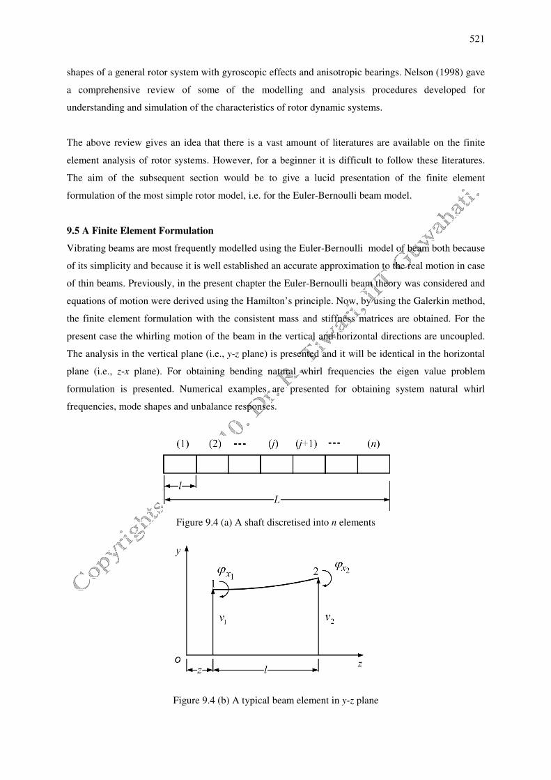
Figure 9.4 (a) A shaft discretised into n elements

Figure 9.4 (b) A typical beam element in y-z plane

522

Let us discretise a given shaft into several finite elements (Fig. 9.4a), and consider an element in the

plane y-z as shown in Figure 9.4b. The element has two nodes 1 and 2. Let v be the nodal linear

displacement and ϕx be the nodal angular displacement of the shaft element. The linear and angular

displacements are acting in the positive axis directions at nodal points and are shown in Figure 9.4.

In the finite element model, continuous displacement variables are approximated in terms of

discretised displacements at nodes of an element. Therefore, the displacement can be expressed within

the element by using appropriate shape functions, as

{ }( )( ) ( , ) ( ) ( )neev z t N z tη= (9.47)

where ( )N z is the row vector of the shape function, { }( )

( )ne

tη is the nodal displacement vector, and

superscripts: (e) and (ne) represent an element and nodes of the element, respectively. Let r be the

number of nodal displacements then the number of shape functions would also be equal to r.

9.5.1 FE Formulation in a weak form

On substituting the approximate elemental solution of equation (9.47) in the equation of motion (9.17)

, the residue is given by

( ) ( ) ( ) *

0 0( , ) ( ) ( )e e e

xxR EI v Av f z t f t z zρ δ′′′′= + − − −�� (9.48)

The residue could be minimized over the element as

( )

0

( ) 0 1,2, ,

l

e

iN z R dz i r= =∫ … (9.49)

where, Ni is the weight function and l is the element length. The Galerkin method is used to minimize

the residue wherein weight functions are assumed to be same as shape functions. On substituting the

residue in the above equation, we get

2 ( ) 2 2 ( )*

0 02 2 2

0

( ) ( , ) ( ) ( ) 0

l e e

i xx

v vN z A EI f x t f t z z dz

t z zρ δ ∂ ∂ ∂

+ − − − = ∂ ∂ ∂

∫ ; i = 1, 2, …, r (9.50)

On rearranging terms in equation (9.50), we get

523

� { }2 ( ) 2 2 ( )

*

0 02 2 2

0 0 0

( , ) ( ) ( ) 0

l l le e

i i xx i

I

II

v vAN dz N EI dz N f z t f t z z dz

t z zρ δ

∂ ∂ ∂+ − + − =

∂ ∂ ∂ ∫ ∫ ∫

�������

; i = 1, 2, …,r

(9.51)

On integrating by parts (so as to equalise the spatial derivative within the integral) the second term of

equation (9.51) and keeping other integrals as the same, we have

2 ( ) 2 ( ) 2 ( ) 2 ( )

2 2 2 2

0 00 0

l ll le e e e

i i xx i xx i xx

v v v vAN dz N EI N EI N EI dz

t z z z zρ

∂ ∂ ∂ ∂ ∂′ ′′+ − +

∂ ∂ ∂ ∂ ∂ ∫ ∫

{ }*

0 0

0

( , ) ( ) ( ) 0

l

iN f z t f t z z dzδ− + − =∫ ; i = 1, 2, …,r (9.52)

The above equation is the weak FE formulation of the governing equation. The completeness and

compatibility requirement of the field variable (i.e., the displacement) could be obtained from the

above equation as follows. The highest order of derivative with respect to z in equation (9.52) is third,

so the completeness of , ,x xv ϕ ϕ ′ and xϕ ′′ is required (i.e., the derivative of displacement up to the same

order). Hence, a polynomial of third degree will be able to satisfy above condition. The highest order

of derivative with respect to z in integral terms of equation (9.52) is second, so the compatibility up to

v and xϕ is required (i.e., the derivative of displacement up to one order less).

9.5.2 Derivations of Shape functions

Expressing the transverse displacement of the element as a function of nodal degrees of freedom,

11 2, ,x

v vϕ and 2xϕ , as

{ }( )( ) ( , ) ( ) ( )neev z t N z tη= (9.53)

with

{ }1 2

( )

1 2( )Tne

x xt v vη ϕ ϕ = ; 1 2 3 4( ) ( ) ( ) ( ) ( )N z N z N z N z N z=

It should be noted that for two-noded element with two-DOF per node, we have total DOFs of the

element as, r = 4. The linear and angular displacements (i.e., 11 2, ,xv vϕ and

2xϕ ) at nodes 1 and 2 of

the element are specified, and these give four boundary conditions for the element from which four

constants in the shape function can be determined uniquely. Let us assume the transverse

displacement v(z) to be a cubic polynomial, which has four coefficients as unknown, to predict the

displacements within the element as

524

1

2( ) 3 2 3 2

1 2 3 4

3

4

( , ) 1e

a

av z t a z a z a z a z z z

a

a

= + + + =

(9.54)

so that

1

( )2( ) 2 2

1 2 3

3

4

( , )( , ) 3 2 3 1 0

ee

x

a

av z tz t a z a z a z z

az

a

ϕ

∂ = = + + = ∂

(9.55)

where 1a ,

2a , 3a , and

4a are constants to be determined from boundary conditions of the element as

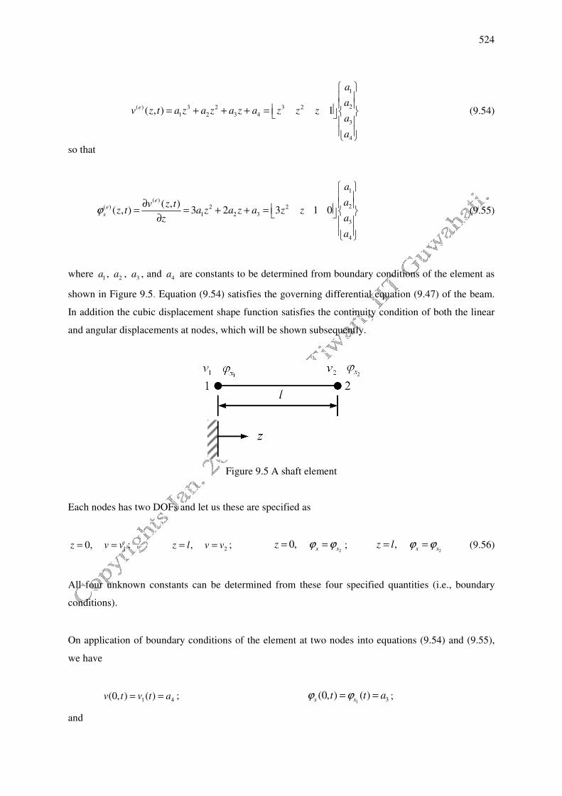
shown in Figure 9.5. Equation (9.54) satisfies the governing differential equation (9.47) of the beam.

In addition the cubic displacement shape function satisfies the continuity condition of both the linear

and angular displacements at nodes, which will be shown subsequently.

Figure 9.5 A shaft element

Each nodes has two DOFs and let us these are specified as

10, z v v= = ; 2, z l v v= = ;

20,

x xz ϕ ϕ= = ;

2,

x xz l ϕ ϕ= = (9.56)

All four unknown constants can be determined from these four specified quantities (i.e., boundary

conditions).

On application of boundary conditions of the element at two nodes into equations (9.54) and (9.55),

we have

1 4(0, ) ( )v t v t a= = ; 1 3(0, ) ( )

x xt t aϕ ϕ= = ;

and

525

3 2

2 1 2 3 4( , ) ( )v l t v t a l a l a l a= = + + + ; 2

2

1 2 3( , ) ( ) 3 2x xl t t a l a l aϕ ϕ= = + + (9.57)

The above could be written in a matrix form, as

[ ]{ } ( ){ ( )} neA a tη= (9.58)

with

[ ] 3 2

3

0 0 0 1

0 0 1 0

1

3 2 1 0

Al l l

l l

=

; { }

1

2

3

4

a

aa

a

a

=

; 1

2

1

( )

2

{ }xne

x

v

v

ϕη

ϕ

=

(9.59)

which can be solved for unknown constants as

1 ( ){ } [ ] { ( )} ne

a A tη−= (9.60)

with

3 2 3 2

2 2

1

2 / 1/ 2 / 1/

3 / 2 / 3 / 1 /[ ]

0 1 0 0

1 0 0 0

l l l l

l l l lA

−

− − − − =

On substituting equation (9.60) into equation (9.54), we get

1

2

( )

1

( ) 3 2 1 ( ) ( )

1 2 3 4

2

( , ) 1 [ ] { ( )} ( ) ( ) ( ) ( ) ( ) { ( )}

ne

xe ne ne

x

v

v z t z z z A t N z N z N z N z N z tv

ϕη η

ϕ

−

= = =

(9.61)

with

2 3 2 3 2 3 2 3

2 3 2 2 3 2( ) 1 3 2 2 3 2

z z z z z z z zN z z

l l l l l l l l

= − + − + − − +

(9.62)

and on substituting equation (9.60) into equation (9.55), we get

526

1

2

( )

1

( ) 2 1 ( ) ( )

1 2 3 4

2

( , ) 3 1 0 [ ] { ( )} ( ) ( ) ( ) ( ) ( ) { ( )}

ne

xe ne ne

x

x

v

z t z z A t N z N z N z N z N z tv

ϕϕ η η

ϕ

−

′ ′ ′ ′ ′ = = =

(9.63)

with

2 2 2 2

2 3 2 2 3 2( ) 6 6 1 4 3 6 6 2 3

z z z z z z z zN z

l l l l l l l l

′ = − + − + − − +

(9.64)

If we define 1ξ and

2ξ as natural coordinates, such that

1 1z

lξ = − and 2

z

lξ = (9.65)

In view of equation (9.65), equations (9.62) and (9.64) will take the following simple form

( ) 3 2 2 2 3 2

1 2 1 2 1 2 1 2 1 2, (3 2 ) 3 2N l lξ ξ ξ ξ ξ ξ ξ ξ ξ ξ = − − − (9.66)

and

( )1 2 2 2

1 1 2 1 2

1

,(9 ) 2 6

Nl l

ξ ξξ ξ ξ ξ ξ

ξ

∂ = − ∂

; ( )1 2 2 2

2 1 2 1 2

2

,( 4 ) 6 2

Nl l

ξ ξξ ξ ξ ξ ξ

ξ

∂ = − − − ∂

(9.67)

The above form of shape functions helps in evaluation of integral relatively easier that is required

frequently at the time of calculation of the elemental mass and stiffness matrices, subsequently.

9.5.3 Satisfaction of the compatibility and completeness conditions

In previous section, we have stated the requirement of the compatibility and completeness conditions

for chosen shape functions. In the present section, we will see whether the chosen cubic polynomial

satisfies these conditions.

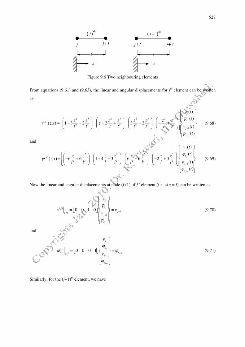
Compatibility Conditions: Consider two neighbouring elements jth and (j+1)

th for checking inter-

element compatibility as shown in Figure 9.6.

527

Figure 9.6 Two neighbouring elements

From equations (9.61) and (9.63), the linear and angular displacements for jth element can be written

as

1

2 3 2 3 2 3 2 3( )

2 3 2 2 3 2

1

( )

( )( , ) 1 3 2 2 3 2

( )

( )

j

j

j

xj

j

x

v t

tz z z z z z z zv z t z

v tl l l l l l l l

t

ϕ

ϕ+

+

= − + − + − − +

(9.68)

and

1

2 2 2 2( )

2 3 2 2 3 2

1

( )

( )( , ) 6 6 1 4 3 6 6 2 3

( )

( )

j

j

j

xj

x

j

x

v t

tz z z z z z z zz t

v tl l l l l l l l

t

ϕϕ

ϕ+

+

= − + − + − − +

(9.69)

Now the linear and angular displacements at node (j+1) of jth element (i.e. at z = l) can be written as

1

( )

1

1

0 0 1 0j

j

j

xj

jz l

j

x

v

v vv

ϕ

ϕ+

+=+

= =

(9.70)

and

1

1

( )

1

0 0 0 1j

j

j

j

xj

x xz l

j

x

v

v

ϕϕ ϕ

ϕ

+

+

=+

= =

(9.71)

Similarly, for the (j+1)th element, we have

528

1

2

1

2 3 2 3 2 3 2 3( 1)

2 3 2 2 3 2

2

( )

( )( , ) 1 3 2 2 3 2

( )

( )

j

j

j

xj

j

x

v t

tz z z z z z z zv z t z

v tl l l l l l l l

t

ϕ

ϕ

+

+

+

+

+

= − + − + − − +

(9.72)

and

1

2

1

2 2 2 2( 1)

2 3 2 2 3 2

2

( )

( )( , ) 6 6 1 4 3 6 6 2 3

( )

( )

j

j

j

xj

x

j

x

v t

tz z z z z z z zz t

v tl l l l l l l l

t

ϕϕ

ϕ

+

+

+

+

+

= − + − + − − +

(9.73)

Now the linear and angular displacements at node (j+1) of (j+1)th element (i.e., at z = 0) can be written

as

1

2

1

( 1)

10

2

1 0 0 0j

j

j

xj

jz

j

x

v

v vv

ϕ

ϕ

+

+

+

++=

+

= =

(9.74)

and

1

1

2

1

1

02

0 1 0 0j

j

j

j

xj

x xz

j

x

v

v

ϕϕ ϕ

ϕ

+

+

+

+

+

=+

= =

(9.75)

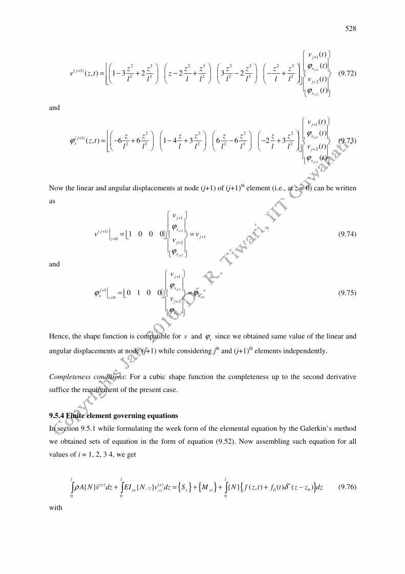
Hence, the shape function is compatible for v and xϕ since we obtained same value of the linear and

angular displacements at node (j+1) while considering jth and (j+1)

th elements independently.

Completeness conditions: For a cubic shape function the completeness up to the second derivative

suffice the requirement of the present case.

9.5.4 Finite element governing equations

In section 9.5.1 while formulating the week form of the elemental equation by the Galerkin’s method

we obtained sets of equation in the form of equation (9.52). Now assembling such equation for all

values of i = 1, 2, 3 4, we get

{ } { } { }( ) ( ) *,

, 0 0

0 0 0

{ } { } { } ( , ) ( ) ( )

l l l

e ezz

xx zz y yzA N v dz EI N v dz S M N f z t f t z z dzρ δ+ = + + + −∫ ∫ ∫�� (9.76)

with

529

{ }

1

2

3

4

N

NN

N

N

=

; { }

1,

2,

,

3,

4,

zz

zz

zz

zz

zz

N

NN

N

N

=

;

{ }

( )

( )

( )

( )

( )

( )

1

2

( )

1 ,, ( )0

,, 0

( )

2 ,, 0

( )( ),3 , ,, 0

( )

4 ,, 0

0

0 0 0

0

00 0

le

xx zzz e

xx zzl z yz

e

xx zzz

y lee y

xx zzxx zz zz z l

le

xx zzz

N EI v

EI v S

N EI v

SS

EI vN EI v

N EI v

=

=

− −

= − = − = − − −

−

;

{ }

( )

( )

( )

( )

( )

( )

1

2

( )

1, ,0

( ) ( )

2, , ,0 0

( )

3, ,0 ( )

,( )

4, ,0

0 00

0

0 0 0

0

le

z xx zz

le e

z xx zz xx zz yzz

yz le

z xx zze

yzxx zzl

z le

z xx zz

N EI v

N EI v EI v MM

N EI vMEI v

N EI v

=

=

−

− −

= = = −

−

and

( )

1

( )

, , 0

e

y xx zz z z

S EI v=

= − ; ( )1

( )

,0

e

yz xx zzz

M EI v=

= ; ( )2

( )

, ,

e

y xx zz z z l

S EI v=

= − and ( )2

( )

,

e

yz xx zzz l

M EI v=

=

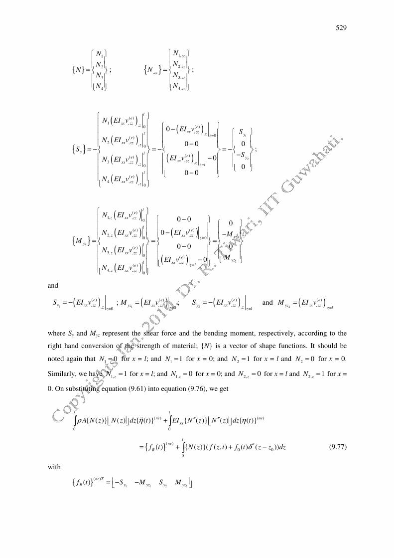
where Sy and Myz represent the shear force and the bending moment, respectively, according to the

right hand conversion of the strength of material; {N} is a vector of shape functions. It should be

noted again that 1 0N = for x = l; and

1 1N = for x = 0; and 2 1N = for x = l and

2 0N = for x = 0.

Similarly, we have 1, 1z

N = for x = l; and 1, 0z

N = for x = 0; and 2, 0z

N = for x = l and 2, 1z

N = for x =

0. On substituting equation (9.61) into equation (9.76), we get

( ) ( )

0 0

{ ( )} ( ) { ( )} { ( )} ( ) { ( )}

l l

ne ne

xxA N z N z dz t EI N z N z dz tρ η η′′ ′′+ ∫ ∫��

{ }( ) *

0 0

0

( ) { ( )}( ( , ) ( ) ( ))

lne

Rf t N z f z t f t z z dzδ= + + −∫ (9.77)

with

{ }1 1 2 2

( )( )

ne T

R y yz y yzf t S M S M = − −

530

Equation (9.77) can be written as

{ } { }( ) ( )( ) ( ) ( ) ( )[ ] ( ) [ ] { ( )} { ( )} ( )ne nee e ne ne

ext RM t K t f t f tη η+ = +�� (9.78)

with

{ } { }1 2

( )

1 2( )

Tne

x xt v vη ϕ ϕ= ; ( ) *

0 0

0

{ ( )} { ( )}( ( , ) ( ) ( ))

l

ne

extf t N z f z t f t z z dzδ= + −∫

where ( )[ ] e

M is the consistent mass matrix of the element, ( )[ ] e

K is the stiffness matrix of the

element, {η(t)} is the generalized force vector, { }( )

( )ne

Rf t is the reactive or internal nodal force

vector, and { }( )

( )ne

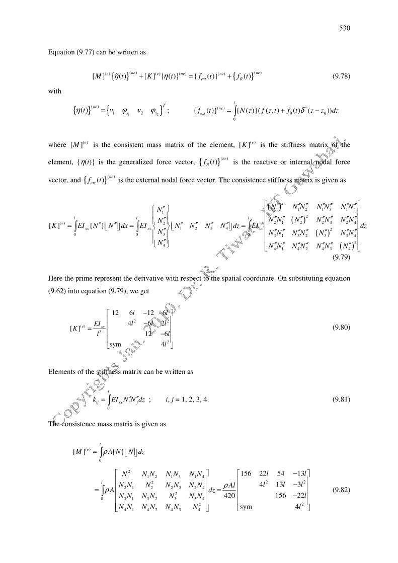
extf t is the external nodal force vector. The consistence stiffness matrix is given as

( )

( )

( )

2

1 1 2 1 3 1 41

2

2 1 2 2 3 2 4( ) 2

1 2 3 4 2

30 0 3 1 3 2 3 3 4

44 1 4 2 4

[ ] { }

l l

e

xx xx xx

N N N N N N NN

N N N N N N NNK EI N N dx EI N N N N dz EI

N N N N N N N N

NN N N N N

′′ ′′ ′′ ′′ ′′ ′′ ′′′′ ′′ ′′ ′′ ′′ ′′ ′′ ′′′′

′′ ′′ ′′ ′′ ′′ ′′= = = ′′ ′′ ′′ ′′ ′′ ′′ ′′ ′′ ′′ ′′ ′′ ′′ ′′ ′′

∫ ∫

( )

0

2

3 4

l

dz

N N

′′ ′′

∫

(9.79)

Here the prime represent the derivative with respect to the spatial coordinate. On substituting equation

(9.62) into equation (9.79), we get

2 2

( )

3

2

12 6 12 6

4 6 2[ ]

12 6

sym 4

e xx

l l

l l lEIK

ll

l

− − = −

(9.80)

Elements of the stiffness matrix can be written as

0

l

ij xx i jk EI N N dz′′ ′′= ∫ ; i, j = 1, 2, 3, 4. (9.81)

The consistence mass matrix is given as

( )

0

[ ] { }

l

eM A N N dzρ= ∫

2

1 1 2 1 3 1 4

2 22

2 1 2 2 3 2 4

2

3 1 3 2 3 3 40

22

4 1 4 2 4 3 4

156 22 54 13

4 13 3

156 22420

sym 4

l

l lN N N N N N N

l l lN N N N N N N AlA dz

lN N N N N N N

lN N N N N N N

ρρ

− − = = −

∫ (9.82)

531

Elements of the mass matrix can be written as

0

l

ij i jm AN N dzρ= ∫ i, j = 1, 2, 3, 4. (9.83)

It should be noted that both the mass and stiffness matrices are symmetric. In should be noted that we

neglected the rotary inertia while deriving the equation of motion of a continuous beam. The rotary

inertia terms appeared in above elemental mass matrix (corresponding to even rows and even

columns) is due to consideration of element as a whole. Damping has not been considered at present

in subsequent sections the Rayleigh’s (or proportionate) damping will be discussed.

9.5.5 The consistent load matrix

In the previous section, we derived finite element equations wherein the consistent mass and stiffness

matrices were also obtained with the help of chosen shape functions. In the present section, we will be

obtaining the consistent force vector for variety of loading conditions.

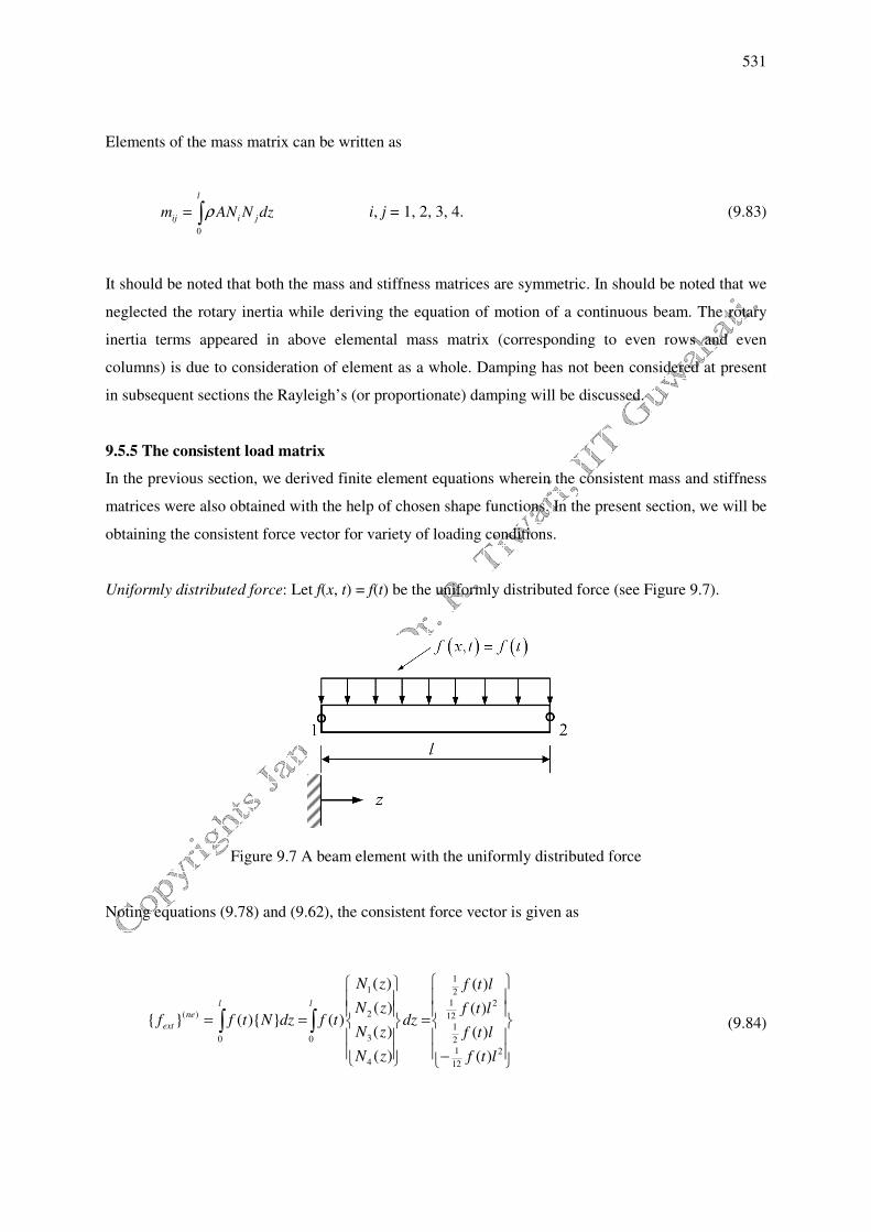
Uniformly distributed force: Let f(x, t) = f(t) be the uniformly distributed force (see Figure 9.7).

Figure 9.7 A beam element with the uniformly distributed force

Noting equations (9.78) and (9.62), the consistent force vector is given as

(9.84)

1

1 2

1 2

2( ) 12

1

30 0 2

1 2

4 12

( ) ( )

( ) ( ){ } ( ){ } ( )

( ) ( )

( ) ( )

l l

ne

ext

N z f t l

N z f t lf f t N dz f t dz

N z f t l

N z f t l

= = =

−

∫ ∫

532

It should be noted that because of the uniformly distributed force over the element both forces and

moments are present at both nodes of the element. In fact total force over the element is f(t)l which is

same as that at nodes of the element, i.e. on adding the first and third columns of the consistent force

vector. In addition to these forces we have moments at the second and third columns. While following

the lumped system approach, one would have distributed the total force equally at nodes without any

moment terms.

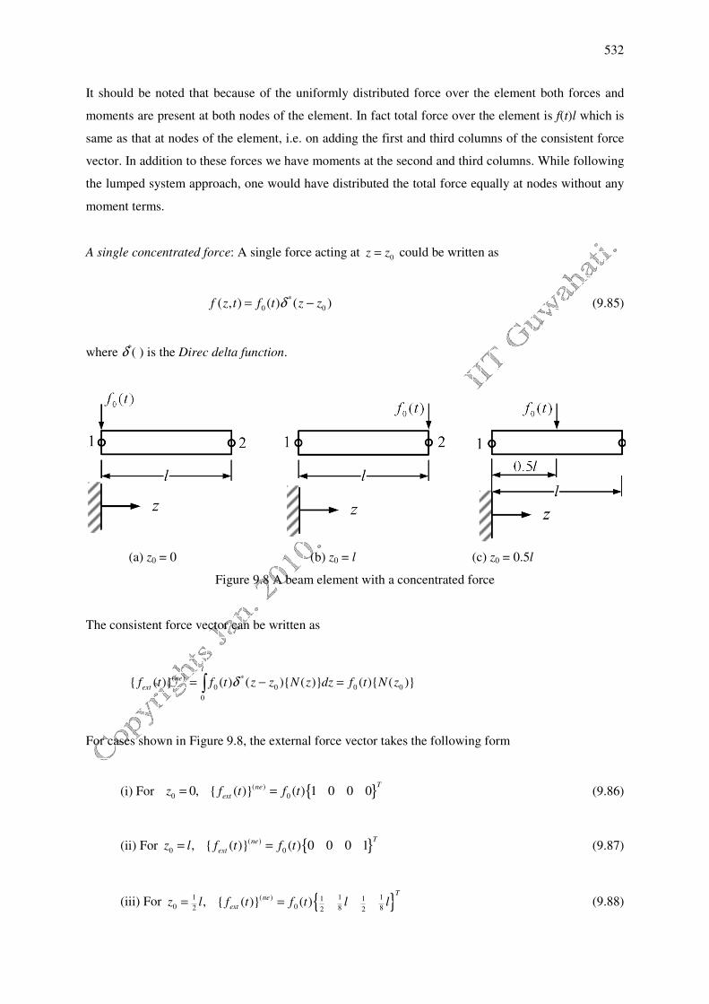
A single concentrated force: A single force acting at 0z z= could be written as

*

0 0( , ) ( ) ( )f z t f t z zδ= − (9.85)

where δ*( ) is the Direc delta function.

(a) z0 = 0 (b) z0 = l (c) z0 = 0.5l

Figure 9.8 A beam element with a concentrated force

The consistent force vector can be written as

( ) *

0 0 0 0

0

{ ( )} ( ) ( ){ ( )} ( ){ ( )}

l

ne

extf t f t z z N z dz f t N zδ= − =∫

For cases shown in Figure 9.8, the external force vector takes the following form

(i) For { }( )

0 00, { ( )} ( ) 1 0 0 0Tne

extz f t f t= = (9.86)

(ii) For { }( )

0 0, { ( )} ( ) 0 0 0 1Tne

extz l f t f t= = (9.87)

(iii) For { }1 1 1( ) 1 10 02 8 82 2

, { ( )} ( )T

ne

extz l f t f t l l= = (9.88)

533

The first and third rows of the force vector represent the equivalent force at nodes of the external force

applied to the element at various locations as shown in Figure 9.8. Similarly, the second and fourth

rows represent the equivalent moment at the nodes due to external force. For cases (i) and (ii) since

the external force is at node 1 or 2, respectively; hence corresponding equivalent force remains the

same. However, for case (iii) the external force is equally distributed at nodes 1 and 2, and apart from

that it produces moments also at both nodes. Hence, a load inside the element will produce equivalent

forces and moments at both the nodes. It is true also while an external moment is applied instead of an

external force.

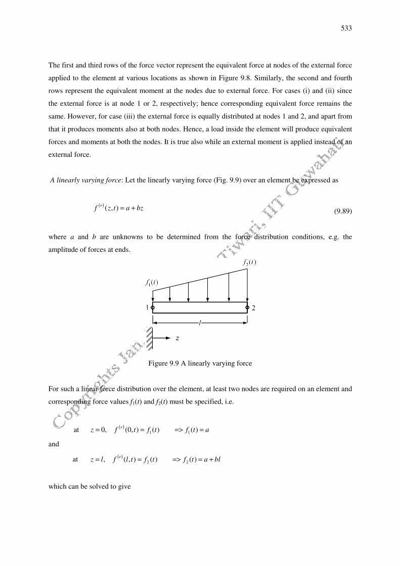
A linearly varying force: Let the linearly varying force (Fig. 9.9) over an element be expressed as

( )( , )

ef z t a bz= + (9.89)

where a and b are unknowns to be determined from the force distribution conditions, e.g. the

amplitude of forces at ends.

Figure 9.9 A linearly varying force

For such a linear force distribution over the element, at least two nodes are required on an element and

corresponding force values f1(t) and f2(t) must be specified, i.e.

( )1 1at 0, (0, ) ( ) ( )

ez f t f t f t a= = => =

and

at ( )2 2, ( , ) ( ) ( )

ez l f l t f t f t a bl= = => = +

which can be solved to give

534

2 11 and

f fa f b

l

−= =

Then, the assumed form of the element force becomes

1( ) ( )2 11

2

( )( ) ( )( , ) ( ) 1 ( ) { ( )}

( )

e ne

f

f tf t f t z zf z t f t z N z f t

f tl l l

− = + = − =

(9.90)

where Nf(z) is the shape function for the force. Hence the consistent load vector would be

( )( )( )

( )

7 3

1 27 3 20 20

20 201 1 2

1 12 21 220 301( ) ( ) 20 30

3 7 3 720 20 20 1 220 20

1 12 2

1 1 230 20

1 230 20

( ) ( )

( ) ( )( ){ ( )} { ( )} ( ) { ( )}

( ) ( ) ( )

( ) ( )

l

ne ne

ext f

f t f t ll l

f t f t lf tl lf t N z N z dz f t

f tl l f t f t l

l lf t f t l

+ +

= = = +

− − − −

∫

(9.91)

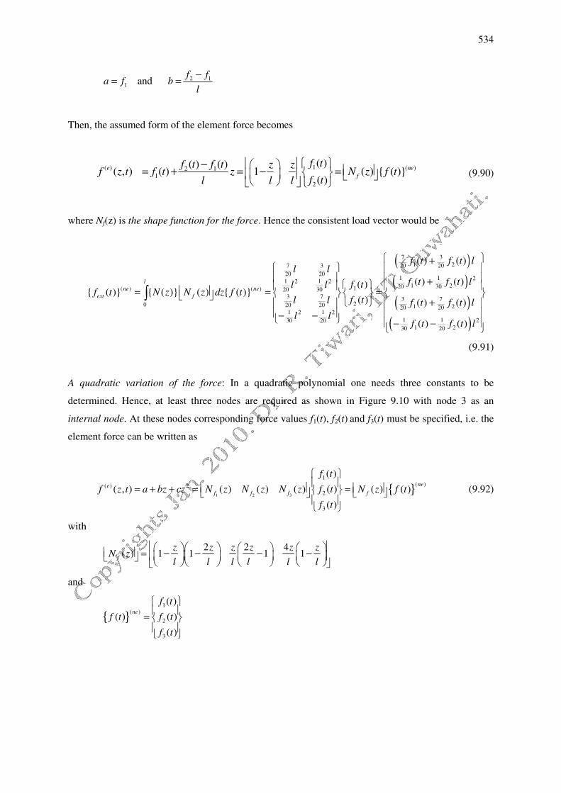
A quadratic variation of the force: In a quadratic polynomial one needs three constants to be

determined. Hence, at least three nodes are required as shown in Figure 9.10 with node 3 as an

internal node. At these nodes corresponding force values f1(t), f2(t) and f3(t) must be specified, i.e. the

element force can be written as

{ }1 2 3

1( )( ) 2

2

3

( )

( , ) ( ) ( ) ( ) ( ) ( ) ( )

( )

nee

f f f f

f t

f z t a bz cz N z N z N z f t N z f t

f t

= + + = =

(9.92)

with

2 2 4( ) 1 1 1 1

f

z z z z z zN z

l l l l l l

= − − − −

and

{ }1

( )

2

3

( )

( ) ( )

( )

ne

f t

f t f t

f t

=

535

Figure 9.10 A beam element with a quadratic variation of the force

Hence, the nodal external force vector is defined as

( ) ( )

0

{ ( )} { ( )} ( ) { ( )}

l

ne ne

ext ff t N z N z dz f t = ∫ (9.93)

To obtain the explicit expression of the same, it is left to the reader as an exercise.

9.5.6 System equations of motion

In previous sections, we have obtained the elemental mass and stiffness matrices, and the internal and

external force vectors. The objective of the present section is to demonstrate how to get system mass

and stiffness matrices and force vectors in terms of the elemental mass and stiffness matrices and

force vectors as given in equation (9.78). To illustrate the same let us take a two-element system with

a rigid disc at node 2 as shown in Figure 9.11(a). Nodal displacement variables are shown in Fig.

9.11(b) at each of the three nodes. In Fig. 9.11(c) two elements are shown with corresponding internal

shear forces and bending moments, where in symbols superscripts specifies the element number and

subscript specifies the node number. Here the disc is assumed to be at node 2 of element 1. The

elemental differential equations for elements 1 and 2, respectively, may be written as

[ ] { }( ) [ ] { } { }

(1) (1)1) (1) (1)

( ) ( ) ( )R

M t K t f tη η+ =�� (9.94)

and

[ ] { } [ ] { } { }(2) (2)(2) (2) (2)

( ) ( ) ( )R

M t K t f tη η+ =�� (9.95)

536

where superscript represent the element number. External forces are not considered.

Figure 9.11 Two-element shaft with a rigid thin disc (a) discretisation of system, (b) nodal generalized

coordinates, and (c) nodal forces and moments in elements.

The mass and stiffness matrices for each of the element are obtained as in equation (9.78). By

considering connectivity between various nodes the corresponding elemental mass and stiffness

matrices are added to get the global mass and stiffness matrices. The elemental stiffness and mass

matrices of equations (9.94) and (9.95), could be stated as follows (note that the point mass m is

assumed to be attached to the element 1 at node 2)

[ ]

(1) (1) (1) (1)

11 12 13 14

(1) (1) (1) (1)(1) 21 22 23 24

(1) (1) (1) (1)

31 32 33 34

(1) (1) (1) (1)

41 42 43 44

k k k k

k k k kK

k k k k

k k k k

=

, [ ]

(2) (2) (2) (2)

33 34 35 36

(2) (2) (2) (2)(2) 43 44 45 46

(2) (2) (2) (2)

53 54 55 56

(2) (2) (2) (2)

63 64 65 66

k k k k

k k k kK

k k k k

k k k k

=

[ ]

(1) (1) (1) (1)

11 12 13 14

(1) (1) (1) (1)(1) 21 22 23 24

(1) (1) (1) (1)

31 32 33 34

(1) (1) (1) (1)

41 42 43 44

( )

m m m m

m m m mM

m m m m m

m m m m

= +

, [ ]

(2) (2) (2) (2)

33 34 35 36

(2) (2) (2) (2)(2) 43 44 45 46

(2) (2) (2) (2)

53 54 55 56

(2) (2) (2) (2)

63 64 65 66

m m m m

m m m mM

m m m m

m m m m

=

With the nodal displacement and internal force vectors are defined as

537

{ } 1

2

1

(1)

2

( )x

x

v

tv

ϕη

ϕ

=

; { } 2

3

2

(2)

3

( )x

x

v

tv

ϕη

ϕ

=

; { }

1

1

2

2

(1)

(1)

(1)

(1)

(1)

( )

y

yz

R

y

yz

S

Mf t

S

M

−

− =

; { }

2

2

3

3

(2)

(2)

(2)

(2)

(2)

( )

y

yz

R

y

yz

S

Mf t

S

M

−

− =

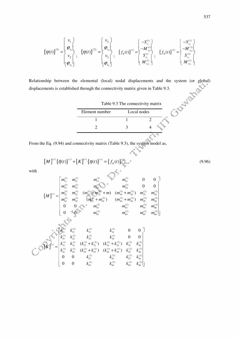
Relationship between the elemental (local) nodal displacements and the system (or global)

displacements is established through the connectivity matrix given in Table 9.3.

Table 9.3 The connectivity matrix

Element number Local nodes

1 1 2

2 3 4

From the Eq. (9.94) and connectivity matrix (Table 9.3), the system model as,

[ ] { } [ ] { } { }( ) ( )( ) ( ) ( )

( ) ( ) ( )s ss s s

RM t K t f tη η+ =�� (9.96)

with

[ ]

(1) (1) (1) (1)

11 12 13 14

(1) (1) (1) (1)

21 22 23 24

(1) (1) (1) (2) (1) (2) (2) (2)( ) 31 32 33 33 34 34 35 36

(1) (1) (1) (2) (1) (2) (2) (2)

41 42 43 43 44 44 45 46

(2) (2) (2) (2)

53 54 55 56

(2

63

0 0

0 0

( ) ( )

( ) ( )

0 0

0 0

s

m m m m

m m m m

m m m m m m m m mM

m m m m m m m m

m m m m

m

+ + +=

+ +

) (2) (2) (2)

64 65 66m m m

[ ]

(1) (1) (1) (1)

11 12 13 14

(1) (1) (1) (1)

21 22 23 24

(1) (1) (1) (2) (1) (2) (2) (2)( ) 31 32 33 33 34 34 35 36

(1) (1) (1) (2) (1) (2) (2) (2)

41 42 43 43 44 44 45 46

(2) (2) (2) (2)

53 54 55 56

(2)

63

0 0

0 0

( ) ( )

( ) ( )

0 0

0 0

s

k k k k

k k k k

k k k k k k k kK

k k k k k k k k

k k k k

k k

+ +=

+ +

(2) (2) (2)

64 65 66k k

538

{ }

1

2

3

1

( ) 2

3

( )

x

s

x

x

v

vt

v

ϕ

ηϕ

ϕ

=

and { }

1 1

1 1

2 2

2 2

3 3

3 3

(1) (1)

(1) (1)

(1) (2)

( )

(1) (2)

(2) (2)

(2) (2)

0( )

0

y y

yz yz

s y y

R

yz yz

y y

yz yz

S S

M M

S Sf t

M M

S S

M M

− −

− − −

= = −

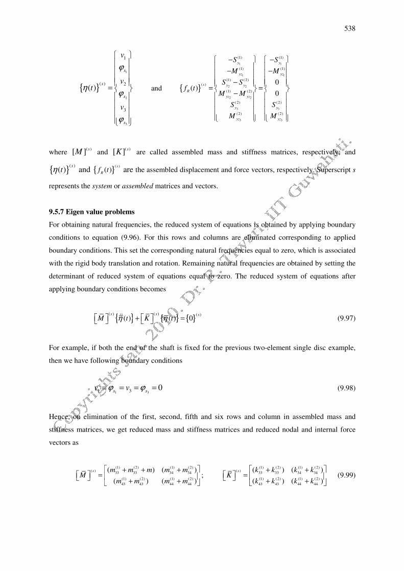
where ( )[ ] s

M

and ( )[ ] s

K are called assembled mass and stiffness matrices, respectively; and

{ }( )

( )s

tη and { }( )

( )s

Rf t are the assembled displacement and force vectors, respectively. Superscript s

represents the system or assembled matrices and vectors.

9.5.7 Eigen value problems

For obtaining natural frequencies, the reduced system of equations is obtained by applying boundary

conditions to equation (9.96). For this rows and columns are eliminated corresponding to applied

boundary conditions. This set the corresponding natural frequencies equal to zero, which is associated

with the rigid body translation and rotation. Remaining natural frequencies are obtained by setting the

determinant of reduced system of equations equal to zero. The reduced system of equations after

applying boundary conditions becomes

{ } { } { }( ) ( ) ( )

( ) ( ) 0s s s

M t K tη η + = �� (9.97)

For example, if both the end of the shaft is fixed for the previous two-element single disc example,

then we have following boundary conditions

1 31 3 0x x

v vϕ ϕ= = = =

(9.98)

Hence, on elimination of the first, second, fifth and six rows and column in assembled mass and

stiffness matrices, we get reduced mass and stiffness matrices and reduced nodal and internal force

vectors as

(1) (2) (1) (2)( )

33 33 34 34

(1) (2) (1) (2)

43 43 44 44

( ) ( )

( ) ( )

s m m m m mM

m m m m

+ + + = + +

;

(1) (2) (1) (2)( )

33 33 34 34

(1) (2) (1) (2)

43 43 44 44

( ) ( )

( ) ( )

s k k k kK

k k k k

+ + = + +

(9.99)

539

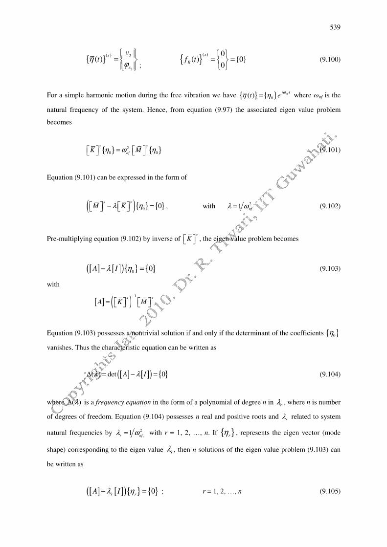
{ }2

( ) 2( )

s

x

vtη

ϕ

= ;

{ }( ) 0

( ) {0}0

s

Rf t

= =

(9.100)

For a simple harmonic motion during the free vibration we have { } { }0( ) nfj tt e

ωη η= where ωnf is the

natural frequency of the system. Hence, from equation (9.97) the associated eigen value problem

becomes

{ } { }2

0 0

s s

nfK Mη ω η = (9.101)

Equation (9.101) can be expressed in the form of

( ){ } { }0 0s s

M Kλ η − = , with 21 nfλ ω= (9.102)

Pre-multiplying equation (9.102) by inverse of s

K , the eigen value problem becomes

[ ] [ ]( ){ } { }00A Iλ η− = (9.103)

with

[ ] ( )1

s s

A K M−

=

Equation (9.103) possesses a nontrivial solution if and only if the determinant of the coefficients { }0η

vanishes. Thus the characteristic equation can be written as

[ ] [ ]( ) { }( ) det 0A Iλ λ∆ = − = (9.104)

where ( )λ∆ is a frequency equation in the form of a polynomial of degree n in rλ , where n is number

of degrees of freedom. Equation (9.104) possesses n real and positive roots and rλ related to system

natural frequencies by 21rr nfλ ω= with r = 1, 2, …, n. If { }rη , represents the eigen vector (mode

shape) corresponding to the eigen value rλ , then n solutions of the eigen value problem (9.103) can

be written as

[ ] [ ]( ){ } { }0r r

A Iλ η− = ; r = 1, 2, …, n (9.105)

540

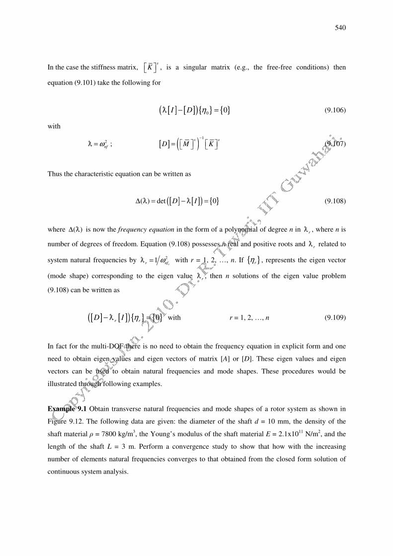
In the case the stiffness matrix, s

K , is a singular matrix (e.g., the free-free conditions) then

equation (9.101) take the following for

[ ] [ ]( ){ } { }00I D η− =� (9.106)

with

2

nfω=� ; [ ] ( )1

s s

D M K−

=

(9.107)

Thus the characteristic equation can be written as

[ ] [ ]( ) { }( ) det 0D I∆ = − =� � (9.108)

where ( )∆ � is now the frequency equation in the form of a polynomial of degree n in r� , where n is

number of degrees of freedom. Equation (9.108) possesses n real and positive roots and r� related to

system natural frequencies by 21rr nfω=� with r = 1, 2, …, n. If { }rη , represents the eigen vector

(mode shape) corresponding to the eigen value r� , then n solutions of the eigen value problem

(9.108) can be written as

[ ] [ ]( ){ } { }0r r

D I η− =� with r = 1, 2, …, n (9.109)

In fact for the multi-DOF there is no need to obtain the frequency equation in explicit form and one

need to obtain eigen values and eigen vectors of matrix [A] or [D]. These eigen values and eigen

vectors can be used to obtain natural frequencies and mode shapes. These procedures would be

illustrated through following examples.

Example 9.1 Obtain transverse natural frequencies and mode shapes of a rotor system as shown in

Figure 9.12. The following data are given: the diameter of the shaft d = 10 mm, the density of the

shaft material ρ = 7800 kg/m3, the Young’s modulus of the shaft material E = 2.1x10

11 N/m

2, and the

length of the shaft L = 3 m. Perform a convergence study to show that how with the increasing

number of elements natural frequencies converges to that obtained from the closed form solution of

continuous system analysis.

541

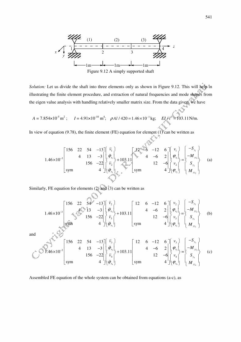
Figure 9.12 A simply supported shaft

Solution: Let us divide the shaft into three elements only as shown in Figure 9.12. This will help in

illustrating the finite element procedure, and extraction of natural frequencies and mode shapes from

the eigen value analysis with handling relatively smaller matrix size. From the data given, we have

A = 7.854×10-5

m2 ; I = 4.91×10

-10 m

4; 3/ 420 1.46 10Alρ −= × kg; 3/ 103.11EI l = N/m.

In view of equation (9.78), the finite element (FE) equation for element (1) can be written as

1

1 1 1

2

2 2 2

1 1

3

2 2

156 22 54 13 12 6 12 6

4 13 3 4 6 21.46 10 103.11

156 22 12 6

sym 4 sym 4

y

x x yz

y

x x yz

Sv v

M

v v S

M

ϕ ϕ

ϕ ϕ

−

− − − −− − × + =

− −

��

��

��

��

(a)

Similarly, FE equation for elements (2) and (3) can be written as

2

22 2

3

3 3 3

2 2

3

3 3

156 22 54 13 12 6 12 6

4 13 3 4 6 21.46 10 103.11

156 22 12 6

sym 4 sym 4

y

yzx x

y

x x yz

Sv v

M

Sv v

M

ϕ ϕ

ϕ ϕ

−

− − − −− − × + =

− −

��

��

��

��

(b)

and

3

3 3 3

4

4 4 4

3 3

3

4 4

156 22 54 13 12 6 12 6

4 13 3 4 6 21.46 10 103.11

156 22 12 6

sym 4 sym 4

y

x x yz

y

x x yz

Sv v

M

v v S

M

ϕ ϕ

ϕ ϕ

−

− − − −− − × + =

− −

��

��

��

��

(c)

Assembled FE equation of the whole system can be obtained from equations (a-c), as

542

1

2

3

4

1

2

3

3

4

156 22 54 13 0 0 0 0 12 6 12 6 0 0 0 0

4 13 3 0 0 0 0 4 6 2 0 0 0 0

312 0 54 13 0 0 24 0 12 6 0 0

8 13 3 0 01.46 10 103.11

312 0 54 13

8 13 3

156 22

sym 4

x

x

x

x

v

v

v

v

ϕ

ϕ

ϕ

ϕ

−

− − − − − − × + − − −

��

��

��

��

��

��

��

��

1

1 1

2

3

4

44

1

2

3

4

0

8 6 2 0 0 0

24 0 12 6 0

8 6 2 0

12 6

sym 4

y

x yz

x

x

y

yzx

v S

M

v

v

Sv

M

ϕ

ϕ

ϕ

ϕ

− − = − − −

(d)

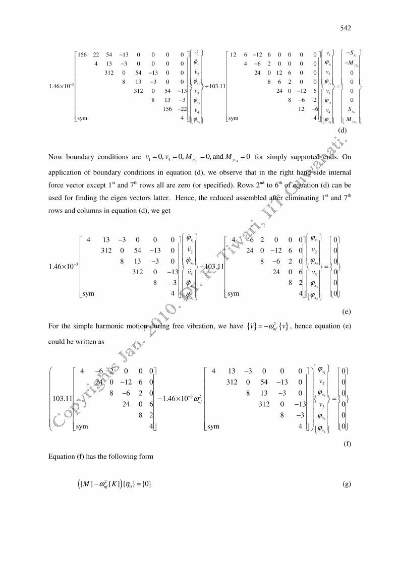
Now boundary conditions are 1 41 40, 0, 0, and 0

yz yzv v M M= = = = for simply supported ends. On

application of boundary conditions in equation (d), we observe that in the right hand side internal

force vector except 1st and 7

th rows all are zero (or specified). Rows 2

nd to 6

th of equation (d) can be

used for finding the eigen vectors latter. Hence, the reduced assembled after eliminating 1st and 7

th

rows and columns in equation (d), we get

1 1

2 2

3 3

4 4

2 2

3

3 3

4 13 3 0 0 0 4 6 2 0 0 0

312 0 54 13 0 24 0 12 6 0

8 13 3 0 8 6 2 01.46 10 103.11

312 0 13 24 0 6

8 3 8 2

sym 4 sym 4

x x

x x

x x

x x

v v

v v

ϕ ϕ

ϕ ϕ

ϕ ϕ

ϕ ϕ

−

− − − − − −

× + −

−

��

��

��

��

��

��

0

0

0

0

0

0

=

(e)

For the simple harmonic motion during free vibration, we have { } { }2

nfv vω= −�� , hence equation (e)

could be written as

1

2

3

4

2

3 2

3

4 6 2 0 0 0 4 13 3 0 0 0 0

24 0 12 6 0 312 0 54 13 0 0

8 6 2 0 8 13 3 0 0103.11 1.46 10

24 0 6 312 0 13 0

8 2 8 3 0

sym 4 sym 4 0

x

x

nf

x

x

v

v

ϕ

ϕω

ϕ

ϕ

−

− − − − − −

− × = −

−

(f)

Equation (f) has the following form

( )2

0[ ] [ ] { } {0}nf

M Kω η− = (g)

543

Which has the eigen value problem of the following form

( ) 0[ ] [ ] { } {0}A I η− =� with A = [K]-1

[M] and 2

nfω=� (h)

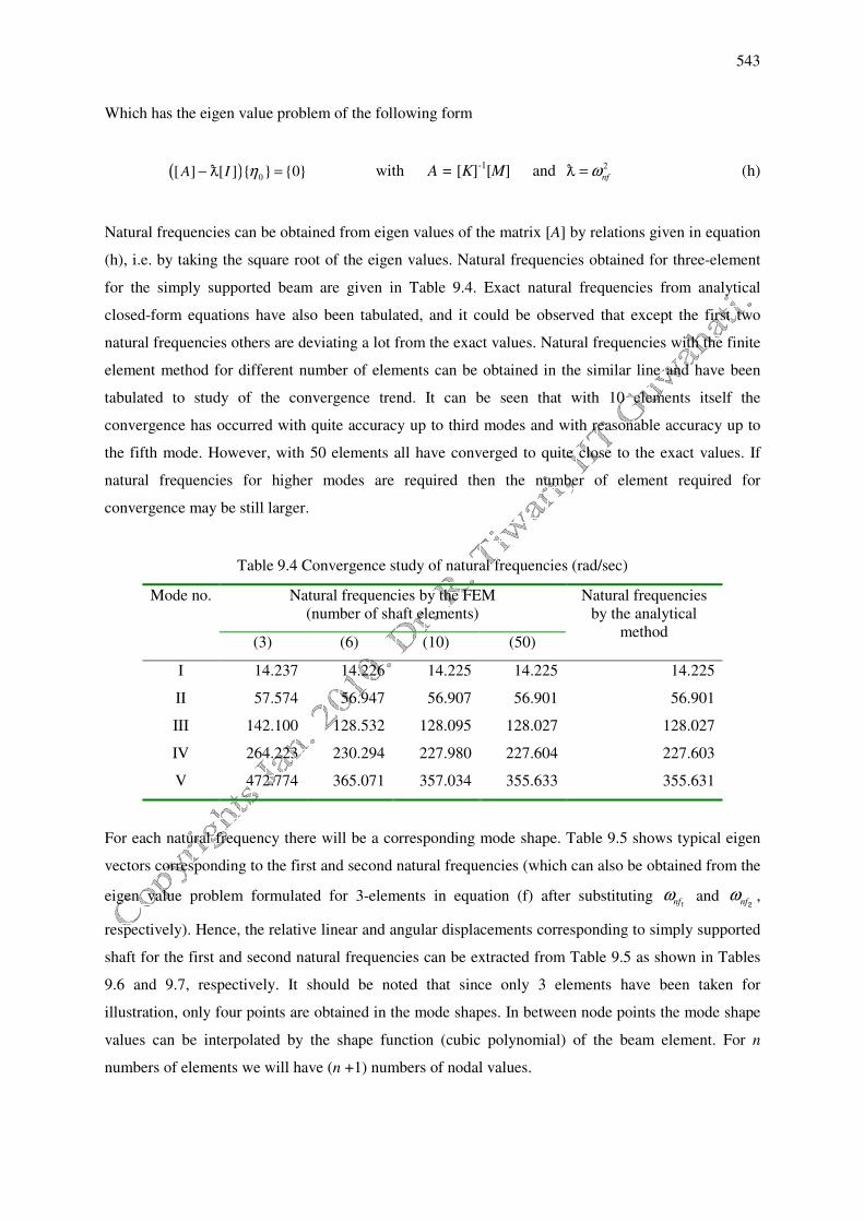
Natural frequencies can be obtained from eigen values of the matrix [A] by relations given in equation

(h), i.e. by taking the square root of the eigen values. Natural frequencies obtained for three-element

for the simply supported beam are given in Table 9.4. Exact natural frequencies from analytical

closed-form equations have also been tabulated, and it could be observed that except the first two

natural frequencies others are deviating a lot from the exact values. Natural frequencies with the finite

element method for different number of elements can be obtained in the similar line and have been

tabulated to study of the convergence trend. It can be seen that with 10 elements itself the

convergence has occurred with quite accuracy up to third modes and with reasonable accuracy up to

the fifth mode. However, with 50 elements all have converged to quite close to the exact values. If

natural frequencies for higher modes are required then the number of element required for

convergence may be still larger.

Table 9.4 Convergence study of natural frequencies (rad/sec)

Mode no.

Natural frequencies by the FEM

(number of shaft elements)

Natural frequencies

by the analytical

method (3) (6) (10) (50)

I 14.237 14.226 14.225 14.225 14.225

II 57.574 56.947 56.907 56.901 56.901

III 142.100 128.532 128.095 128.027 128.027

IV 264.223 230.294 227.980 227.604 227.603

V 472.774 365.071 357.034 355.633 355.631

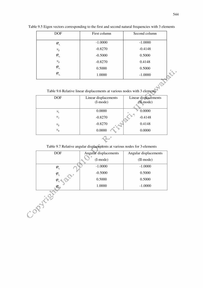
For each natural frequency there will be a corresponding mode shape. Table 9.5 shows typical eigen

vectors corresponding to the first and second natural frequencies (which can also be obtained from the

eigen value problem formulated for 3-elements in equation (f) after substituting nfω

1 and nf

ω2

,

respectively). Hence, the relative linear and angular displacements corresponding to simply supported

shaft for the first and second natural frequencies can be extracted from Table 9.5 as shown in Tables

9.6 and 9.7, respectively. It should be noted that since only 3 elements have been taken for

illustration, only four points are obtained in the mode shapes. In between node points the mode shape

values can be interpolated by the shape function (cubic polynomial) of the beam element. For n

numbers of elements we will have (n +1) numbers of nodal values.

544

Table 9.5 Eigen vectors corresponding to the first and second natural frequencies with 3 elements

Table 9.6 Relative linear displacements at various nodes with 3 elements

DOF Linear displacements

(I-mode)

Linear displacements

(II-mode)

v1

2v

v3

v4

0.0000

-0.8270

-0.8270

0.0000

0.0000

-0.4148

0.4148

0.0000

Table 9.7 Relative angular displacements at various nodes for 3-elements

DOF Angular displacements

(I-mode)

Angular displacements

(II-mode)

1xϕ

2xϕ

3xϕ

4xϕ

-1.0000

-0.5000

0.5000

1.0000

-1.0000

0.5000

0.5000

-1.0000

DOF First column Second column

1xϕ

v2

2xϕ

v3

3xϕ

4xϕ

-1.0000

-0.8270

-0.5000

-0.8270

0.5000

1.0000

-1.0000

-0.4148

0.5000

0.4148

0.5000

-1.0000

545

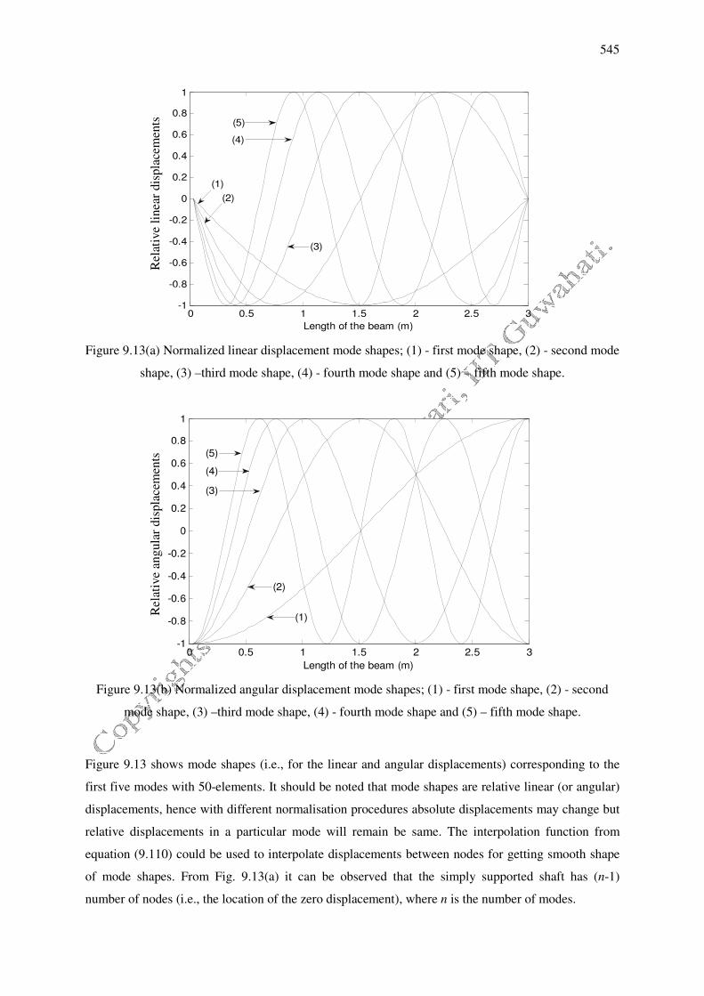
Figure 9.13(a) Normalized linear displacement mode shapes; (1) - first mode shape, (2) - second mode

shape, (3) –third mode shape, (4) - fourth mode shape and (5) – fifth mode shape.

Figure 9.13(b) Normalized angular displacement mode shapes; (1) - first mode shape, (2) - second

mode shape, (3) –third mode shape, (4) - fourth mode shape and (5) – fifth mode shape.

Figure 9.13 shows mode shapes (i.e., for the linear and angular displacements) corresponding to the

first five modes with 50-elements. It should be noted that mode shapes are relative linear (or angular)

displacements, hence with different normalisation procedures absolute displacements may change but

relative displacements in a particular mode will remain be same. The interpolation function from

equation (9.110) could be used to interpolate displacements between nodes for getting smooth shape

of mode shapes. From Fig. 9.13(a) it can be observed that the simply supported shaft has (n-1)

number of nodes (i.e., the location of the zero displacement), where n is the number of modes.

0 0.5 1 1.5 2 2.5 3-1

-0.8

-0.6

-0.4

-0.2

0

0.2

0.4

0.6

0.8

1

Length of the beam (m)

(1)

(2)

(3)

(5)

(4)

0 0.5 1 1.5 2 2.5 3-1

-0.8

-0.6

-0.4

-0.2

0

0.2

0.4

0.6

0.8

1

Length of the beam (m)

(5)

(4)

(3)

(2)

(1)

Rel

ativ

e li

nea

r dis

pla

cem

ents

R

elat

ive

ang

ula

r dis

pla

cem

ents

546

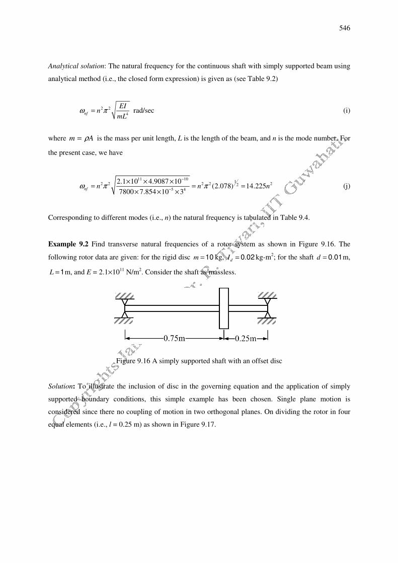
Analytical solution: The natural frequency for the continuous shaft with simply supported beam using

analytical method (i.e., the closed form expression) is given as (see Table 9.2)

2 2

4nf

EIn

mLω π= rad/sec (i)

where Am ρ= is the mass per unit length, L is the length of the beam, and n is the mode number. For

the present case, we have

11 10

12 2 2 2 22

5 4

2.1 10 4.9087 10(2.078) 14.225

7800 7.854 10 3nf n n nω π π

−

−

× × ×= = =

× × × (j)

Corresponding to different modes (i.e., n) the natural frequency is tabulated in Table 9.4.

Example 9.2 Find transverse natural frequencies of a rotor system as shown in Figure 9.16. The

following rotor data are given: for the rigid disc m = 10 kg, .dI = 0 02 kg-m2; for the shaft .d = 0 01m,

L =1m, and E = 2.1×1011

N/m2. Consider the shaft as massless.

Figure 9.16 A simply supported shaft with an offset disc

Solution: To illustrate the inclusion of disc in the governing equation and the application of simply

supported boundary conditions, this simple example has been chosen. Single plane motion is

considered since there no coupling of motion in two orthogonal planes. On dividing the rotor in four

equal elements (i.e., l = 0.25 m) as shown in Figure 9.17.

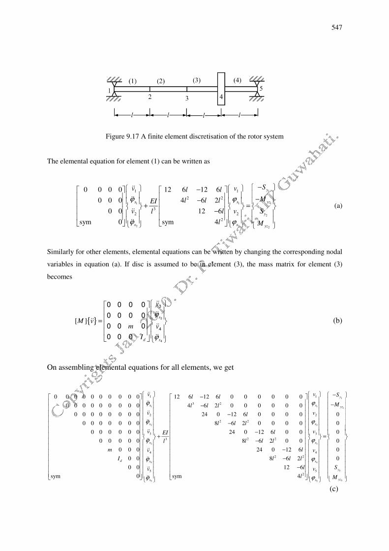
547

Figure 9.17 A finite element discretisation of the rotor system

The elemental equation for element (1) can be written as

1

1 1 1

2

2 2 2

1 1

2 2

3

2 2

2

0 0 0 0 12 6 12 6

0 0 0 4 6 2

0 0 12 6

sym 0 sym 4

y

x x yz

y

x x yz

Sv vl l

Ml l lEI

v l v Sl

l M

ϕ ϕ

ϕ ϕ

− − −− + =

−

��

��

��

��

(a)

Similarly for other elements, elemental equations can be written by changing the corresponding nodal

variables in equation (a). If disc is assumed to be in element (3), the mass matrix for element (3)

becomes

{ }[ ]x

d x

v

M vm v

I

ϕ

ϕ

=

��

����

��

��

3

4

3

4

0 0 0 0

0 0 0 0

0 0 0

0 0 0

(b)

On assembling elemental equations for all elements, we get

1

2

3

4

5

1

3 2

2

3

3

4

5

0 0 0 0 0 0 0 0 0 0 12 6 12 6 0 0 0 0 0 0

0 0 0 0 0 0 0 0 0 4 6 2 0

0 0 0 0 0 0 0 0

0 0 0 0 0 0 0

0 0 0 0 0 0

0 0 0 0 0

0 0 0

0 0

0 0

sym 0

x

x

x

d x

x

v l l

l l l

v

v EI

l

m v

I

v

ϕ

ϕ

ϕ

ϕ

ϕ

− −

+

��

��

��

��

��

��

��

��

��

��

1

11

2

3

4

5

55

1

2

2 2

3

2 2

4

2 2

52

0 0 0 0 0

024 0 12 6 0 0 0 0

08 6 2 0 0 0 0

024 0 12 6 0 0

08 6 2 0 0

024 0 12 6

08 6 2

12 6

sym 4

y

x yz

x

x

x

y

yzx

v S

M

vl

l l l

vl

l l l

l v

l l l

Sl v

l M

ϕ

ϕ

ϕ

ϕ

ϕ

− − − − −

= −

− − −

(c)

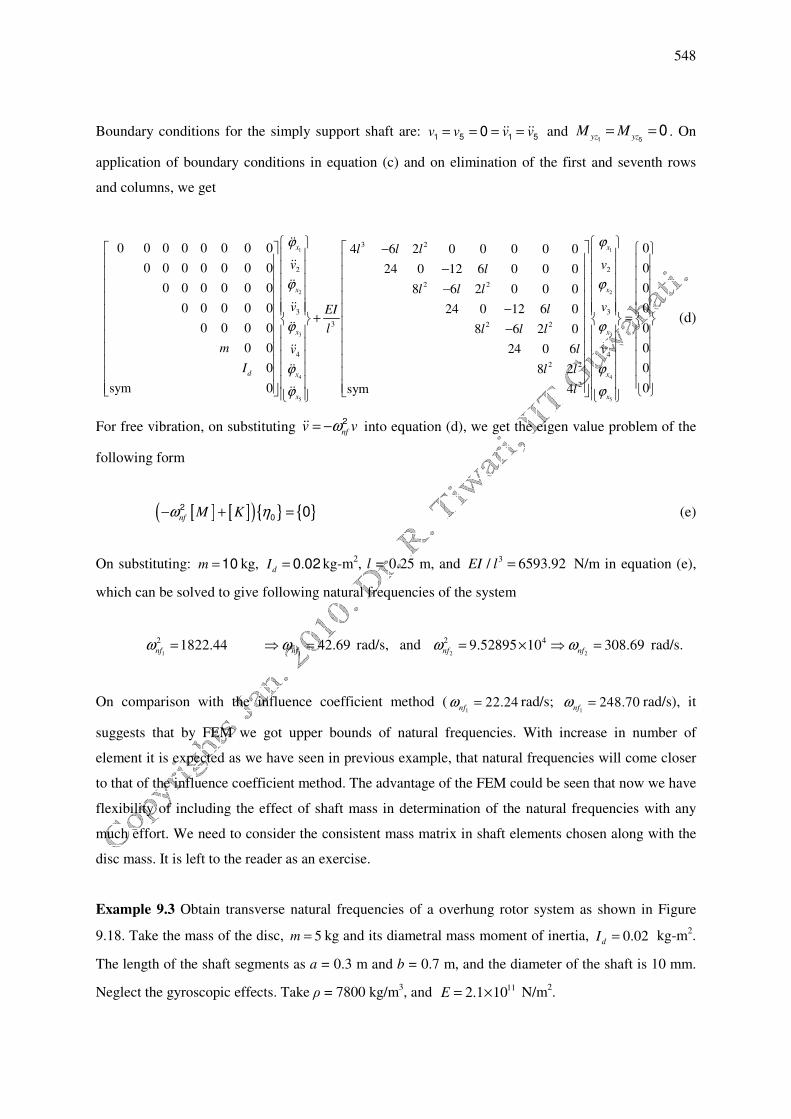
548

Boundary conditions for the simply support shaft are: v v v v= = = =1 5 1 50 �� �� and yz yzM M= =

1 50 . On

application of boundary conditions in equation (c) and on elimination of the first and seventh rows

and columns, we get

1

2

3

4

5

3 2

2

2 2

3

3 2 2

4

0 0 0 0 0 0 0 0 4 6 2 0 0 0 0 0

0 0 0 0 0 0 0 24 0 12 6 0 0 0

0 0 0 0 0 0 8 6 2 0 0 0

0 0 0 0 0 24 0 12 6 0

0 0 0 0 8 6 2 0

0 0 24 0 6

0 8

sym 0

x

x

x

d x

x

l l l

v l

l l l

v lEI

l l l l

m lv

I

ϕ

ϕ

ϕ

ϕ

ϕ

− − − − + −

��

��

��

��

��

��

��

��

1

2

3

4

5

2

3

4

2 2

2

0

0

0

0

0

0

02

0sym 4

x

x

x

x

x

v

v

v

l l

l

ϕ

ϕ

ϕ

ϕ

ϕ

=

(d)

For free vibration, on substituting nfv vω= −�� 2 into equation (d), we get the eigen value problem of the

following form

[ ] [ ]( ){ } { }nfM Kω η− + =2

0 0 (e)

On substituting: m = 10 kg, .dI = 0 02 kg-m2, l = 0.25 m, and 3/ 6593.92EI l = N/m in equation (e),

which can be solved to give following natural frequencies of the system

1 1

2 1822.44 42.69nf nfω ω= ⇒ = rad/s, and 2 2

2 49.52895 10 308.69nf nfω ω= × ⇒ = rad/s.

On comparison with the influence coefficient method (1

22.24nf

ω = rad/s; 1

248.70nf

ω = rad/s), it

suggests that by FEM we got upper bounds of natural frequencies. With increase in number of

element it is expected as we have seen in previous example, that natural frequencies will come closer

to that of the influence coefficient method. The advantage of the FEM could be seen that now we have

flexibility of including the effect of shaft mass in determination of the natural frequencies with any

much effort. We need to consider the consistent mass matrix in shaft elements chosen along with the

disc mass. It is left to the reader as an exercise.

Example 9.3 Obtain transverse natural frequencies of a overhung rotor system as shown in Figure

9.18. Take the mass of the disc, 5m = kg and its diametral mass moment of inertia, kg-m2.

The length of the shaft segments as a = 0.3 m and b = 0.7 m, and the diameter of the shaft is 10 mm.

Neglect the gyroscopic effects. Take ρ = 7800 kg/m3, and N/m

2.

0.02dI =

112.1 10E = ×

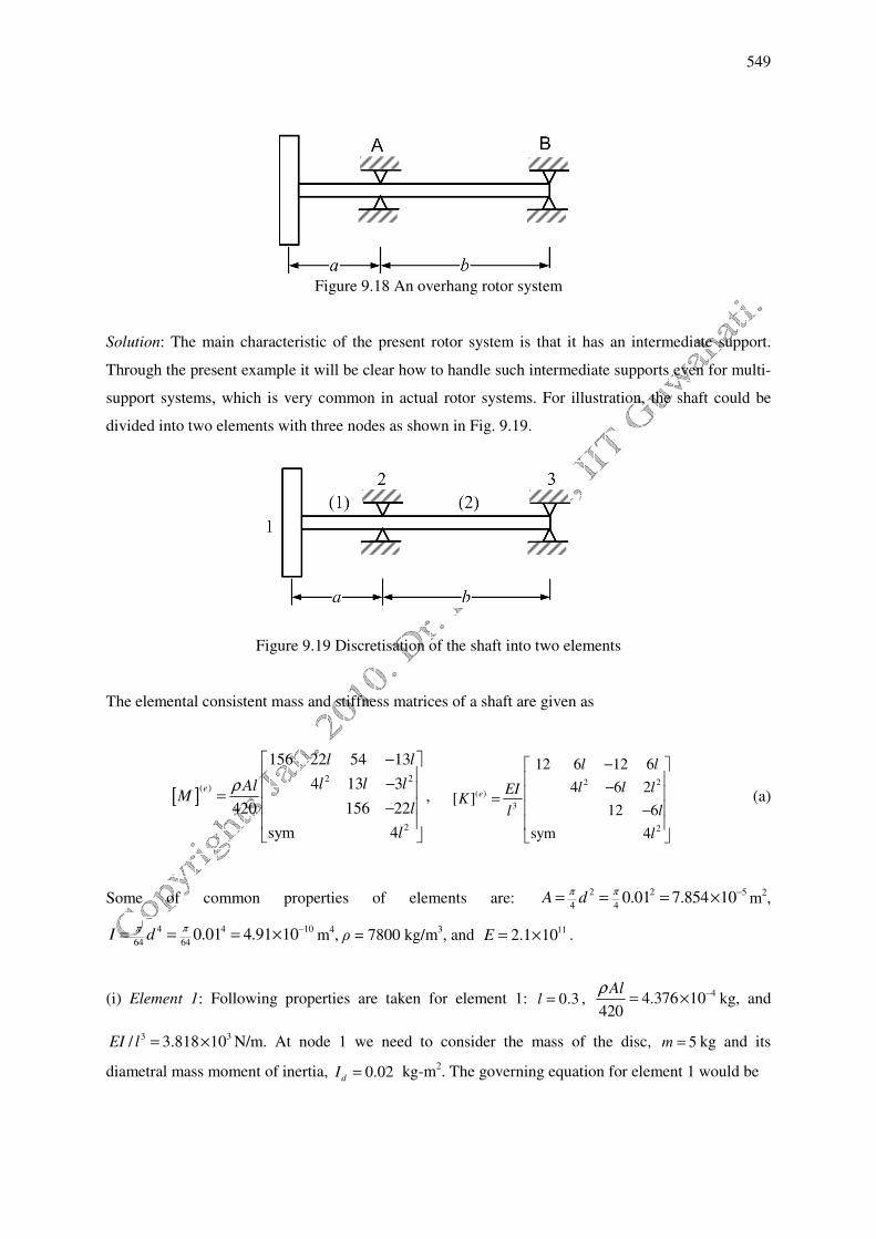
549

Figure 9.18 An overhang rotor system

Solution: The main characteristic of the present rotor system is that it has an intermediate support.

Through the present example it will be clear how to handle such intermediate supports even for multi-

support systems, which is very common in actual rotor systems. For illustration, the shaft could be

divided into two elements with three nodes as shown in Fig. 9.19.

Figure 9.19 Discretisation of the shaft into two elements

The elemental consistent mass and stiffness matrices of a shaft are given as

[ ]2 2

( )

2

156 22 54 13

4 13 3

156 22420

sym 4

e

l l

l l lAlM

l

l

ρ

− − = −

, 2 2

( )

3

2

12 6 12 6

4 6 2[ ]

12 6

sym 4

e

l l

l l lEIK

ll

l

− − = −

(a)

Some of common properties of elements are: 2 2 5

4 40.01 7.854 10A d

π π −= = = × m2,

4 4 10

64 640.01 4.91 10I d

π π −= = = × m4, ρ = 7800 kg/m

3, and .

(i) Element 1: Following properties are taken for element 1: 0.3l = , 44.376 10

420

Alρ −= × kg, and

3 3/ 3.818 10EI l = × N/m. At node 1 we need to consider the mass of the disc, 5m = kg and its

diametral mass moment of inertia, kg-m2. The governing equation for element 1 would be

112.1 10E = ×

0.02dI =

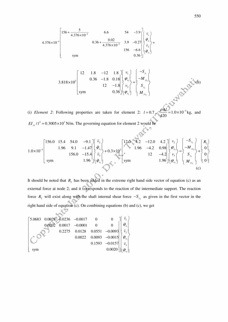
550

1

2

41

4

4

2

5156 6.6 54 3.9

4.376 10

0.020.36 3.9 0.274.376 10

4.376 10

156 6.6

sym 0.36

x

x

v

v

ϕ

ϕ

−

−−

+ − ×

+ −× + ×

−

��

��

��

��

1

1 1

2

2 2

1

3

2

12 1.8 12 1.8

0.36 1.8 0.183.818 10

12 1.8

sym 0.36

y

x yz

y

x yz

Sv

M

v S

M

ϕ

ϕ

− − −− × =

−

(b)

(i) Element 2: Following properties are taken for element 2: 0.7l = , 31.0 10

420

Alρ −= × kg, and

3 3/ 0.3005 10yyEI l = × N/m. The governing equation for element 2 would be

2

22 2

3

3 3 3

2 2

3 3

3 3

156.0 15.4 54.0 9.1 12.0 4.2 12.0 4.2

1.96 9.1 1.47 1.96 4.2 0.981.0 10 0.3 10

156.0 15.4 12 4.2

sym 1.96 sym 1.96

y

yzx x

y

x x yz

Sv v

M

Sv v

M

ϕ ϕ

ϕ ϕ

−

− − − −− − × + × =

− −

��

��

��

��

2

0

0

0

R

+

(c)

It should be noted that 2R has been added in the extreme right hand side vector of equation (c) as an

external force at node 2; and it corresponds to the reaction of the intermediate support. The reaction

force 2R will exist along with the shaft internal shear force

2yS− as given in the first vector in the

right hand side of equation (c). On combining equations (b) and (c), we get

1

2

3

1

2

3

5.0683 0.0029 0.0236 0.0017 0 0

0.0202 0.0017 0.0001 0 0

0.2275 0.0128 0.0551 0.0093

0.0022 0.0093 0.0015

0.1593 0.0157

sym 0.0020

x

x

x

v

v

v

ϕ

ϕ

ϕ

− − −

−

−

��

��

��

��

��

��

551

+

1

1 1

2

3

3 3

1

24

3

4.5815 0.6872 4.5815 0.6872 0 0

0.1374 0.6872 0.0687 0 0

04.9421 0.5610 0.3606 0.126210

00.1963 0.1262 0.0295

0.3606 0.1262

sym 0.0589

y

x yz

x

y

x yz

Sv

M

v

Sv

M

ϕ

ϕ

ϕ

− − −− − −

× = −

−

2

0

0

0

0

0

R

+

(d)

It can be seen from equation (d) that at node 2, the shaft internal reaction forces and moments get

cancelled on assembling of elemental equations. However, the reaction force,2R , from the

intermediate support, which is unknown, will exist in the assembled equation (d). On the assembled

equation is ready for application of the boundary conditions.

Boundary conditions of the present problem are given as follows:

At node 1: 1 1

0y yz

S M= = ; At node 2: 2 0v = ; At node 3:

33 0x

v ϕ= = (e)

It should be noted that at node 2 bending moment will not be zero as in the case of node 3 because

node 2 is an intermediate support and node 3 is a simply support. On application of boundary

conditions, on the right hand side of equation (e) forces R2 and 3y

S will remain non-zero in third and

fifth rows. Hence, by eliminating corresponding 3rd

and 5th rows and columns, equation (e) reduces to

1 1

2 2

3 3

1 1

4

5.0683 0.0029 0.0017 0 4.5815 0.6872 0.6872 0 0

0.0202 1.18 0 0.1374 0.687 0 010

0.0022 0.0015 0.1963 0.0295 0

sym 0.0020 sym 0.0589 0

x x

x x

x x

v v

ϕ ϕ

ϕ ϕ

ϕ ϕ

− − + =

−

��

��

��

��

(f)

For a simple harmonic motion during free vibrations, equation (f) can be written as a standard eigen

value problem as follows

[ ] [ ]( ){ } { }2

0 0nf

D Iω η− = (g)

with

[ ]

5.0683 0.0029 0.0017 0

0.0202 1.18 0

0.0022 0.0015

sym 0.0020

M

− − = −

, [ ] 4

4.5815 0.6872 0.6872 0

0.1374 0.687 010

0.1963 0.0295

sym 0.0589

K

=

(h)

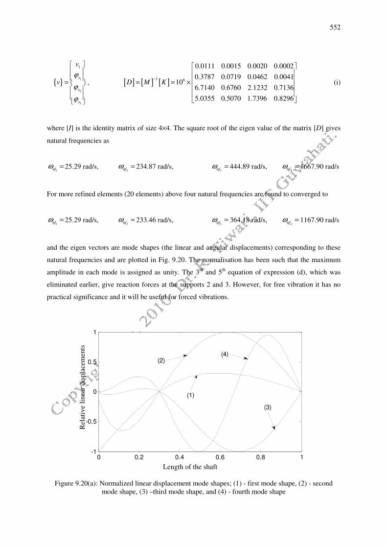
552

{ }1

2

3

1

x

x

x

v

vϕ

ϕ

ϕ

=

, [ ] [ ] [ ]1 6

0.0111 0.0015 0.0020 0.0002

0.3787 0.0719 0.0462 0.004110

6.7140 0.6760 2.1232 0.7136

5.0355 0.5070 1.7396 0.8296

D M K−

= = ×

(i)

where [I] is the identity matrix of size 4×4. The square root of the eigen value of the matrix [D] gives

natural frequencies as

1nfω = 25.29 rad/s,

2nfω = 234.87 rad/s,

3nfω = 444.89 rad/s,

4nfω = 1667.90 rad/s

For more refined elements (20 elements) above four natural frequencies are found to converged to

1nfω = 25.29 rad/s,

2nfω = 233.46 rad/s,

3nfω = 364.18 rad/s,

4nfω = 1167.90 rad/s

and the eigen vectors are mode shapes (the linear and angular displacements) corresponding to these

natural frequencies and are plotted in Fig. 9.20. The normalisation has been such that the maximum

amplitude in each mode is assigned as unity. The 3rd

and 5th equation of expression (d), which was

eliminated earlier, give reaction forces at the supports 2 and 3. However, for free vibration it has no

practical significance and it will be useful for forced vibrations.

Figure 9.20(a): Normalized linear displacement mode shapes; (1) - first mode shape, (2) - second

mode shape, (3) –third mode shape, and (4) - fourth mode shape

0 0.2 0.4 0.6 0.8 1-1

-0.5

0

0.5

1

(1)

(3)

(4)(2)

Rel

ativ

e li

nea

r dis

pla

cem

ents

Length of the shaft

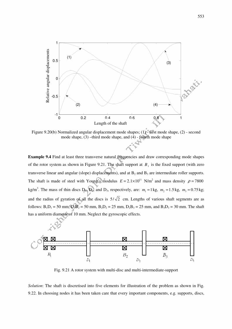
553

Figure 9.20(b) Normalized angular displacement mode shapes; (1) - first mode shape, (2) - second

mode shape, (3) –third mode shape, and (4) - fourth mode shape

Example 9.4 Find at least three transverse natural frequencies and draw corresponding mode shapes

of the rotor system as shown in Figure 9.21. The shaft support at 1B is the fixed support (with zero

transverse linear and angular (slope) displacements), and at B2 and B3 are intermediate roller supports.

The shaft is made of steel with Young’s modulus 112.1 10E = × N/m2 and mass density 7800ρ =

kg/m3. The mass of thin discs D1, D2, and D3, respectively, are:

1 1m = kg, 2 1.5m = kg,

3 0.75m = kg;

and the radius of gyration of all the discs is 5 / 2 cm. Lengths of various shaft segments are as

follows: B1D1 = 50 mm, D1B2 = 50 mm, B2D2 = 25 mm, D2B3 = 25 mm, and B3D3 = 30 mm. The shaft

has a uniform diameter of 10 mm. Neglect the gyroscopic effects.

Fig. 9.21 A rotor system with multi-disc and multi-intermediate-support

Solution: The shaft is discretised into five elements for illustration of the problem as shown in Fig.

9.22. In choosing nodes it has been taken care that every important components, e.g. supports, discs,

0 0.2 0.4 0.6 0.8 1-1

-0.5

0

0.5

1

(1)

(2)

(3)

(4)

Rel

ativ

e an

gula

r dis

pla

cem

ents

Length of the shaft

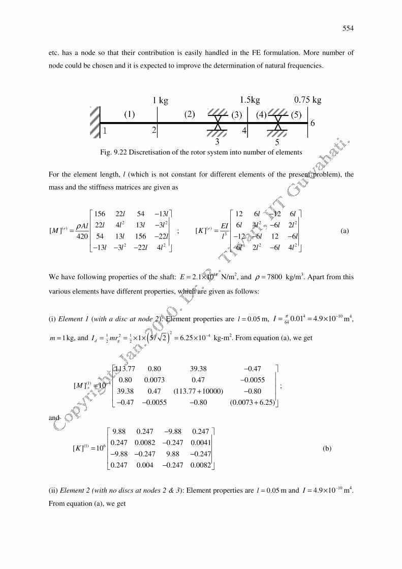
554

etc. has a node so that their contribution is easily handled in the FE formulation. More number of

node could be chosen and it is expected to improve the determination of natural frequencies.

Fig. 9.22 Discretisation of the rotor system into number of elements

For the element length, l (which is not constant for different elements of the present problem), the

mass and the stiffness matrices are given as

2 2

( )

2 2

156 22 54 13

22 4 13 3[ ]

54 13 156 22420

13 3 22 4

e

l l

l l l lAlM

l l

l l l l

ρ

− − = − − − −

;

2 2

( )

3

2 2

12 6 12 6

6 4 6 2[ ]

12 6 12 6

6 2 6 4

e

l l

l l l lEIK

l ll

l l l l

− − = − − −

−

(a)

We have following properties of the shaft: 112.1 10E = × N/m2, and 7800ρ = kg/m

3. Apart from this

various elements have different properties, which are given as follows:

(i) Element 1 (with a disc at node 2): Element properties are 0.05l = m, 4 10

640.01 4.9 10I

π −= = × m4,

1m = kg, and ( )2

1 12 4

2 21 5 / 2 6.25 10d gI mr

−= = × × = × kg-m

2. From equation (a), we get

(1) 4

113.77 0.80 39.38 0.47

0.80 0.0073 0.47 0.0055[ ] 10

39.38 0.47 (113.77 10000) 0.80

0.47 0.0055 0.80 (0.0073 6.25)

M −

− − = + −

− − − +

;

and

(1) 6

9.88 0.247 9.88 0.247

0.247 0.0082 0.247 0.0041[ ] 10

9.88 0.247 9.88 0.247

0.247 0.004 0.247 0.0082

K

− − = − − −

−

(b)

(ii) Element 2 (with no discs at nodes 2 & 3): Element properties are 0.05l = m and 104.9 10I−= × m

4.

From equation (a), we get

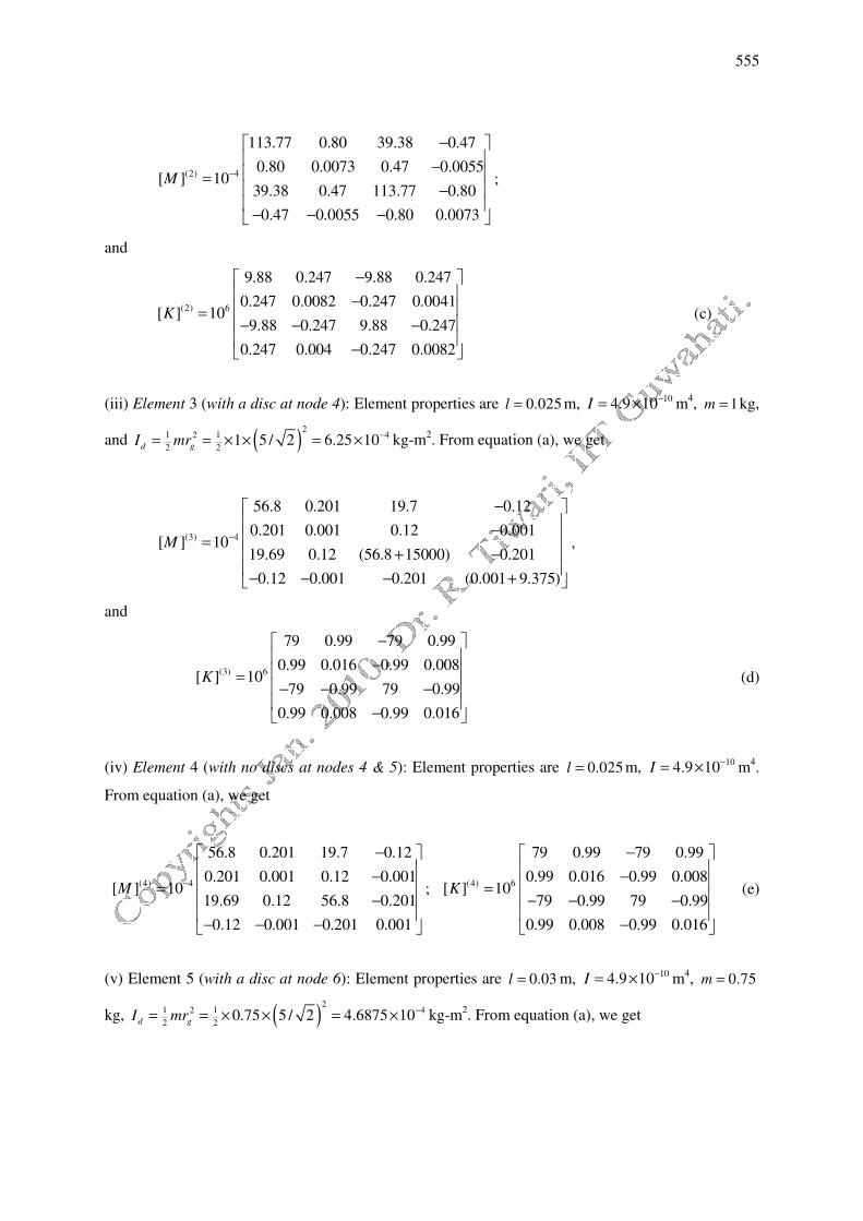
555

(2) 4

113.77 0.80 39.38 0.47

0.80 0.0073 0.47 0.0055[ ] 10

39.38 0.47 113.77 0.80

0.47 0.0055 0.80 0.0073

M −

− − = −

− − −

;

and

(2) 6

9.88 0.247 9.88 0.247

0.247 0.0082 0.247 0.0041[ ] 10

9.88 0.247 9.88 0.247

0.247 0.004 0.247 0.0082

K

− − = − − −

−

(c)

(iii) Element 3 (with a disc at node 4): Element properties are 0.025l = m, 104.9 10I−= × m

4, 1m = kg,

and ( )2

1 12 4

2 21 5 / 2 6.25 10d gI mr

−= = × × = × kg-m2. From equation (a), we get

(3) 4

56.8 0.201 19.7 0.12

0.201 0.001 0.12 0.001[ ] 10

19.69 0.12 (56.8 15000) 0.201

0.12 0.001 0.201 (0.001 9.375)

M −

− − = + − − − − +

,

and

(3) 6

79 0.99 79 0.99

0.99 0.016 0.99 0.008[ ] 10

79 0.99 79 0.99

0.99 0.008 0.99 0.016

K

− − = − − −

−

(d)

(iv) Element 4 (with no discs at nodes 4 & 5): Element properties are 0.025l = m, 104.9 10I−= × m

4.

From equation (a), we get

(4) 4

56.8 0.201 19.7 0.12

0.201 0.001 0.12 0.001[ ] 10

19.69 0.12 56.8 0.201

0.12 0.001 0.201 0.001

M −

− − = − − − −

; (4) 6

79 0.99 79 0.99

0.99 0.016 0.99 0.008[ ] 10

79 0.99 79 0.99

0.99 0.008 0.99 0.016

K

− − = − − −

−

(e)

(v) Element 5 (with a disc at node 6): Element properties are 0.03l = m, 104.9 10I−= × m

4, 0.75m =

kg, ( )2

1 12 4

2 20.75 5 / 2 4.6875 10d gI mr

−= = × × = × kg-m2. From equation (a), we get

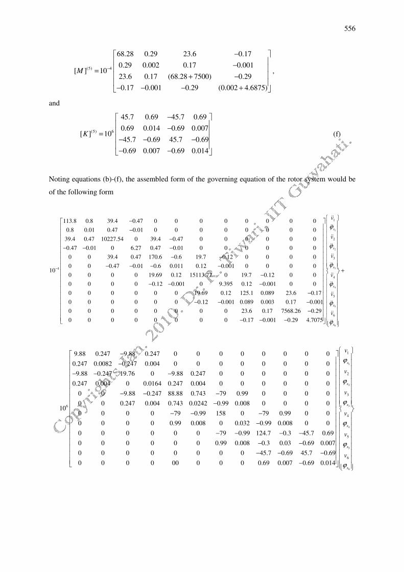
556

(5) 4

68.28 0.29 23.6 0.17

0.29 0.002 0.17 0.001[ ] 10

23.6 0.17 (68.28 7500) 0.29

0.17 0.001 0.29 (0.002 4.6875)

M −

− − = + − − − − +

,

and

(5) 6

45.7 0.69 45.7 0.69

0.69 0.014 0.69 0.007[ ] 10

45.7 0.69 45.7 0.69

0.69 0.007 0.69 0.014

K

− − = − − − − −

(f)

Noting equations (b)-(f), the assembled form of the governing equation of the rotor system would be

of the following form

4

113.8 0.8 39.4 0.47 0 0 0 0 0 0 0 0

0.8 0.01 0.47 0.01 0 0 0 0 0 0 0 0

39.4 0.47 10227.54 0 39.4 0.47 0 0 0 0 0 0

0.47 0.01 0 6.27 0.47 0.01 0 0 0 0 0 0

0 0 39.4 0.47 170.6 0.6 19.7 0.12 0 0 0 0

0 0 0.47 0.01 0.6 0.011 0.12 0.001 0 0 0 010

0 0 0 0 19.69 0.12 15113

−

−

−

−

− − −

− −

− − − −

.77 0 19.7 0.12 0 0

0 0 0 0 0.12 0.001 0 9.395 0.12 0.001 0 0

0 0 0 0 0 0 19.69 0.12 125.1 0.089 23.6 0.17

0 0 0 0 0 0 0.12 0.001 0.089 0.003 0.17 0.001

0 0 0 0 0 0 0 0 23.6 0.17 7568.26 0.29

0 0 0 0 0 0 0 0 0.17 0.001 0.29 4.7075

−

− − − − − − −

− − − −

1

2

3

4

5

6

1

2

3

4

5

6

x

x

x

x

x

x

v

v

v

v

v

v

ϕ

ϕ

ϕ

ϕ

ϕ

ϕ

+

��

��

��

��

��

��

��

��

��

��

��

��

6

9.88 0.247 9.88 0.247 0 0 0 0 0 0 0 0

0.247 0.0082 0.247 0.004 0 0 0 0 0 0 0 0

9.88 0.247 19.76 0 9.88 0.247 0 0 0 0 0 0

0.247 0.004 0 0.0164 0.247 0.004 0 0 0 0 0 0

0 0 9.88 0.247 88.88 0.743 79 0.99 0 0 0 0

0 0 0.247 0.004 0.743 0.0242 0.99 0.008 0 0 0 010

0 0 0

−

−

− − −

− − −

−

0 79 0.99 158 0 79 0.99 0 0

0 0 0 0 0.99 0.008 0 0.032 0.99 0.008 0 0

0 0 0 0 0 0 79 0.99 124.7 0.3 45.7 0.69

0 0 0 0 0 0 0.99 0.008 0.3 0.03 0.69 0.007

0 0 0 0 0 0 0 0 45.7 0.69 45.7 0.69

0 0 0 0 00 0 0 0 0.69 0.007 0.69 0.014

− − −

− − − − − − −

− − − −

1

2

3

4

5

6

1

2

3

4

5

6

x

x

x

x

x

x

v

v

v

v

v

v

ϕ

ϕ

ϕ

ϕ

ϕ

ϕ

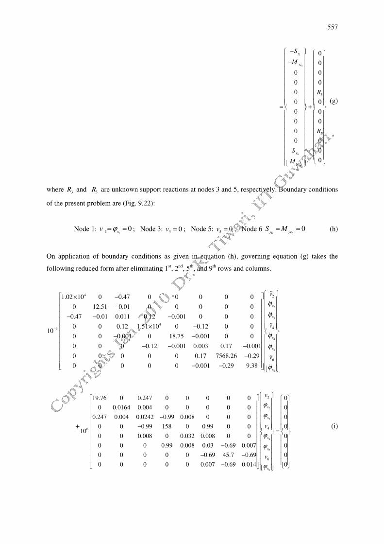
557

1

1

6

6

3

5

0

0

0 0

0 0

0

0 0

0 0

0 0

0

0 0

0

0

y

yz

y

yz

S

M

R

R

S

M

− −

= +

(g)

where 3R and

5R are unknown support reactions at nodes 3 and 5, respectively. Boundary conditions

of the present problem are (Fig. 9.22):

Node 1: 11 0

xv ϕ= = ; Node 3:

3 0v = ; Node 5: 5 0v = ; Node 6

6 60

y yzS M= = (h)

On application of boundary conditions as given in equation (h), governing equation (g) takes the

following reduced form after eliminating 1st, 2

nd, 5

th, and 9

th rows and columns.

4

4

4

1.02 10 0 0.47 0 0 0 0 0

0 12.51 0.01 0 0 0 0 0

0.47 0.01 0.011 0.12 0.001 0 0 0

0 0 0.12 1.51 10 0 0.12 0 010

0 0 0.001 0 18.75 0.001 0 0

0 0 0 0.12 0.001 0.003 0.17 0.001

0 0 0 0 0 0.17 7568.26 0.29

0 0 0 0 0 0.001 0.29 9.38

−

× −

− − − −

× − − −

− − − − − −

2

3

4

5

6

2

4

6

x

x

x

x

x

v

v

v

ϕ

ϕ

ϕ

ϕ

ϕ

��

��

��

��

��

��

��

��

+

2

2

6

19.76 0 0.247 0 0 0 0 0

0 0.0164 0.004 0 0 0 0 0

0.247 0.004 0.0242 0.99 0.008 0 0 0

0 0 0.99 158 0 0.99 0 010

0 0 0.008 0 0.032 0.008 0 0

0 0 0 0.99 0.008 0.03 0.69 0.007

0 0 0 0 0 0.69 45.7 0.69

0 0 0 0 0 0.007 0.69 0.014

x

x

v

ϕ

ϕ

−

−

− − −

−

3

4

5

6

4

6

0

0

0

0

0

0

0

0

x

x

x

v

v

ϕ

ϕ

ϕ

=

(i)

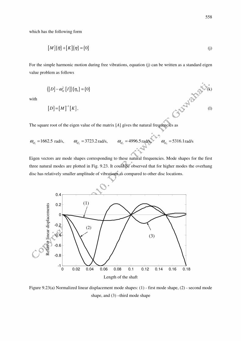
558

which has the following form

[ ]{ } [ ]{ } { }0M Kη η+ =�� (j)

For the simple harmonic motion during free vibrations, equation (j) can be written as a standard eigen

value problem as follows

[ ] [ ]( ){ } { }2

0 0nf

D Iω η− = (k)

with

[ ] [ ] [ ]1

D M K−

= , (l)

The square root of the eigen value of the matrix [A] gives the natural frequencies as

11662.5

nfω = rad/s,

23723.2

nfω = rad/s,

34996.5

nfω = rad/s,

45316.1

nfω = rad/s

Eigen vectors are mode shapes corresponding to these natural frequencies. Mode shapes for the first

three natural modes are plotted in Fig. 9.23. It could be observed that for higher modes the overhang

disc has relatively smaller amplitude of vibrations as compared to other disc locations.

Length of the shaft

Figure 9.23(a) Normalized linear displacement mode shapes: (1) - first mode shape, (2) - second mode

shape, and (3) –third mode shape

0 0.02 0.04 0.06 0.08 0.1 0.12 0.14 0.16 0.18-1

-0.8

-0.6

-0.4

-0.2

0

0.2

0.4

Rel

ativ

e li

nea

r dis

pla

cem

ents

(1)

(2)

(3)

559

Length of the shaft

Figure 9.23(b) Normalized angular displacement mode shapes: (1) - first mode shape, (2) - second

mode shape, and (3) –third mode shape

Example 9.5 A typical simply supported multi-disc rotor system as shown in Figure 9.24 is analyzed

to show the application of the present finite element model. Physical properties of the rotor bearing

system are given as: the diameter of the shaft = 0.1 m, the length of the shaft = 3.5 m, the Young’s

modulus of the shaft material = 2.08×1011

N/m2, the mass density of the shaft material = 7830 kg/m

3,

the number of rigid discs = 4 and the mass of each rigid disc = 60.3 kg. Shaft segments between two

neighbouring discs, between a bearing and a neighbouring disc, and overhang portion are of 0.5m

length each.

Solution: The rotor is modelled as the seven-element and fourteen-element as shown in Figures 9.24

and 9.25, respectively. In the case of seven-element member: (i) identical rigid bearings are located at

node numbers two and seven and (ii) rigid discs are located at node numbers three, four, five and six.

In the case of fourteen-element member: (i) identical rigid bearings are located at node numbers three

and thirteen, and (ii) rigid discs are located at node numbers five, seven, nine and eleven. The shaft

has uniform cross section. Rigid discs are considered as point masses and the mass of the shaft is also

considered. First four transverse natural frequencies are obtained for chosen models and are given in

Table 9.9. Results show that not much improvement in natural frequencies occurred in 14-element

model as compared to 7-element model and it suggest that convergence has already occurred with 7

elements model. Mode shapes are shown in Figure 9.26.

0 0.02 0.04 0.06 0.08 0.1 0.12 0.14 0.16 0.18-1

-0.5

0

0.5

1

Rel

ativ

e an

gula

r dis

pla

cem

ents

(1)

(2) (3)

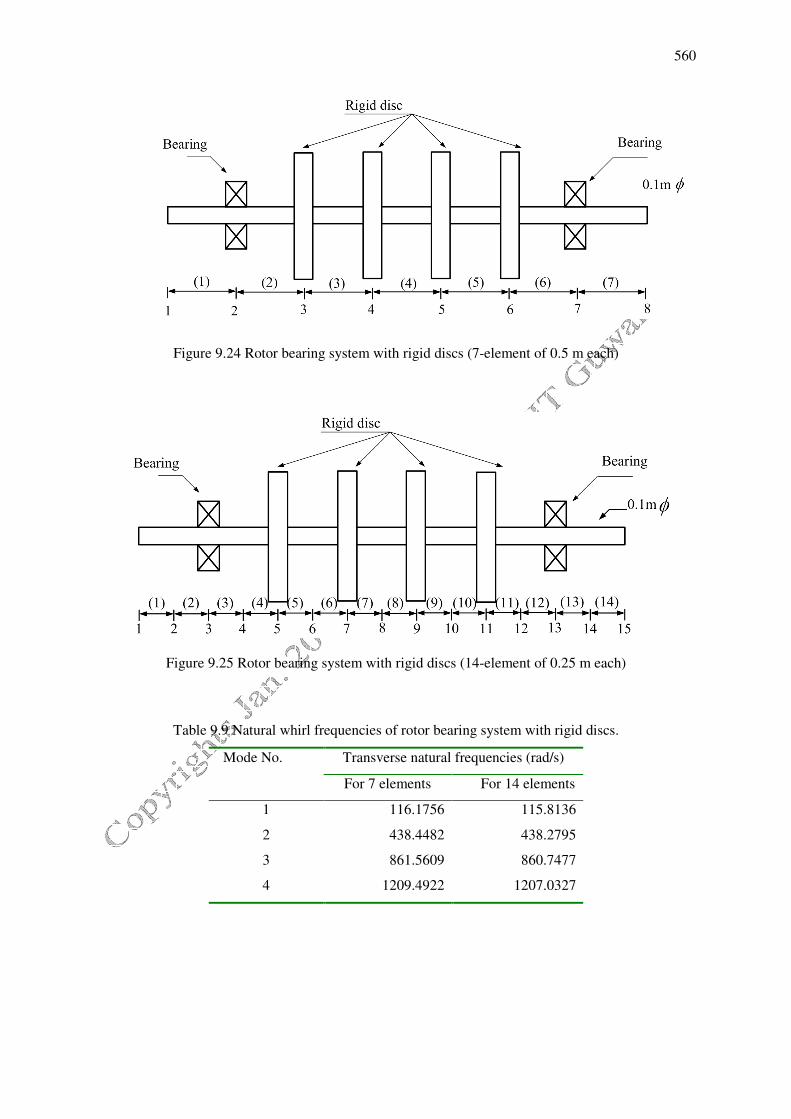
560

Figure 9.24 Rotor bearing system with rigid discs (7-element of 0.5 m each)

Figure 9.25 Rotor bearing system with rigid discs (14-element of 0.25 m each)

Table 9.9 Natural whirl frequencies of rotor bearing system with rigid discs.

Mode No.

Transverse natural frequencies (rad/s)

For 7 elements For 14 elements

1 116.1756 115.8136

2 438.4482 438.2795

3 861.5609 860.7477

4 1209.4922 1207.0327

561

Figure 9.26 Mode shapes for rotor bearing system with rigid discs

Example 9.6 Perform the forced vibration analysis of a rotor system as shown in Figure 9.27. The

shaft has the diameter of d = 10 mm and the disc has the mass of mdisc = 1.5 kg (ignore the diametral

mass moment of inertia of the disc). The unbalance in the disc is given as: munb = 0.005 kg, runb = 0.05

m, and θunb = 300 phase. Plot the unbalance response (i.e. the amplitude and the phase) variation with

respect to the speed of the rotor at the disc location. Choose the upper limit of the speed of the rotor

such that plots should depict first two critical speeds.

Figure 9.27 A single disc rotor system

Solution: The shaft element is taken such that the disc is always at a node point. Figure 9.27 shows the

discretised rotor system with three elements. It is assumed the disc is on element 2. The phase is

measured with respect to some physical reference on the shaft. Let us assume that the reference mark

is aligned with y-axis at time t = 0. The angular speed, ω, is in the counter-clockwise direction as seen

in Figure 9.28. In the present case both the plane motion would be considered simultaneously.

Figure 9.28 A unbalance on the disc at time t

-1.5

-1

-0.5

0

0.5

1

1.5

1 2 3 4 5 6 7 8

Norm

alis

ed E

igen

-Vec

tors

Node Number

Mode I-116.1756

rad/sec

Mode II- 438.4482

rad/sec

Mode III-861.5609

rad/sec

Mode IV-1209.4922

rad/sec

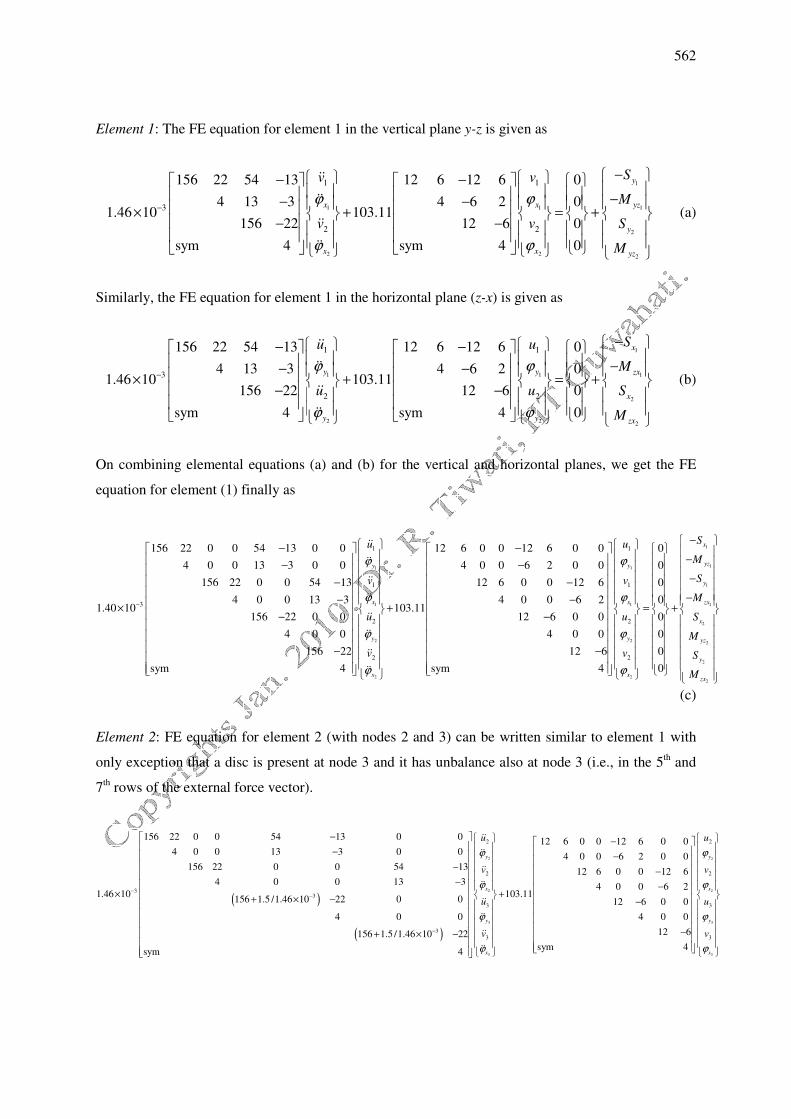
562

Element 1: The FE equation for element 1 in the vertical plane y-z is given as

1

1 1 1

2

2 2 2

1 1

3

2 2

156 22 54 13 12 6 12 6 0

4 13 3 4 6 2 01.46 10 103.11

156 22 12 6 0

sym 4 sym 4 0

y

x x yz

y

x x yz

Sv v

M

v v S

M

ϕ ϕ

ϕ ϕ

−

− − − −− − × + = +

− −

��

��

��

��

(a)

Similarly, the FE equation for element 1 in the horizontal plane (z-x) is given as

1

1 1 1

2

2 2 2

1 1

3

2 2

156 22 54 13 12 6 12 6 0

4 13 3 4 6 2 01.46 10 103.11

156 22 12 6 0

sym 4 sym 4 0

x

y y zx

x

y y zx

Su u

M

u u S

M

ϕ ϕ

ϕ ϕ

−

− − − −− − × + = +

− −

��

��

��

��

(b)

On combining elemental equations (a) and (b) for the vertical and horizontal planes, we get the FE

equation for element (1) finally as

1

1

2

2

1

1

3

2

2

156 22 0 0 54 13 0 0 12 6 0 0 12 6 0 0

4 0 0 13 3 0 0 4 0 0 6 2 0 0

156 22 0 0 54 13 12 6 0 0 12 6

4 0 0 13 3 4 0 0 61.40 10 103.11

156 22 0 0

4 0 0

156 22

sym 4

y

x

y

x

u

v

u

v

ϕ

ϕ

ϕ

ϕ

−

− − − − − −

− − × + − −

��

��

��

��

��

��

��

��

1

11

1

1 1

2

2 2

2

22

1

1

2

2

0

0

0

2 0

12 6 0 0 0

4 0 0 0

12 6 0

sym 4 0

x

yzy

y

x zx

x

y yz

y

xzx

Su

M

Sv

M

u S

M

v S

M

ϕ

ϕ

ϕ

ϕ

− − − − = + − −

(c)

Element 2: FE equation for element 2 (with nodes 2 and 3) can be written similar to element 1 with

only exception that a disc is present at node 3 and it has unbalance also at node 3 (i.e., in the 5th and

7th rows of the external force vector).

( )

( )

2

2

3

3

2

2

33

3

3

3

156 22 0 0 54 13 0 012 6

4 0 0 13 3 0 0

156 22 0 0 54 13

4 0 0 13 3

1.46 10 103.11156 1.5 /1.46 10 22 0 0

4 0 0

156 1.5 /1.46 10 22

sym 4

y

x

y

x

u

v

u

v

ϕ

ϕ

ϕ

ϕ

−−

−

− − − −

× + + × − + × −

��

��

��

��

��

��

��

��

2

2

3

3

2

2

3

3

0 0 12 6 0 0

4 0 0 6 2 0 0

12 6 0 0 12 6

4 0 0 6 2

12 6 0 0

4 0 0

12 6

sym 4

y

x

y

x

u

v

u

v

ϕ

ϕ

ϕ

ϕ

− − −

− − −

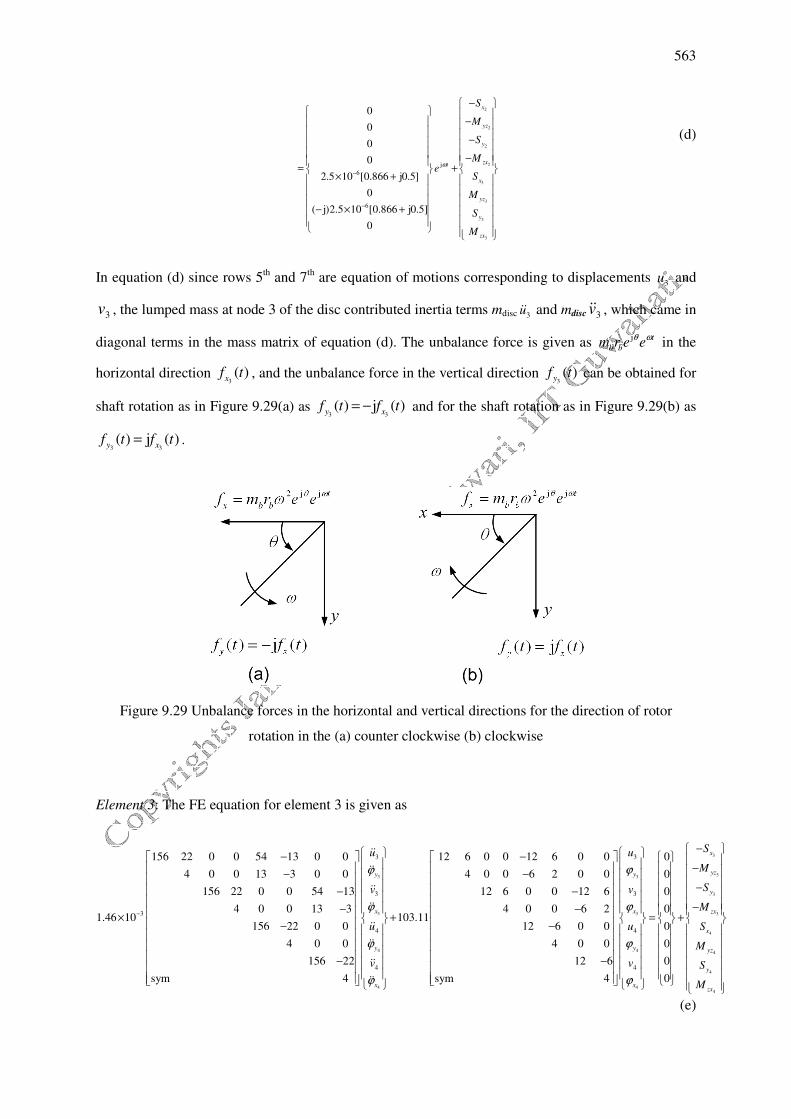
563

2

2

2

2

3

3

3

3

j

6

6

0

0

0

0

2.5 10 [0.866 j0.5]

0

( j)2.5 10 [0.866 j0.5]

0

x

yz

y

zxt

x

yz

y

zx

S

M

S

Me

S

M

S

M

ω−

−

−

− − −

= + × +

− × +

(d)

In equation (d) since rows 5th and 7

th are equation of motions corresponding to displacements

3u and

3v , the lumped mass at node 3 of the disc contributed inertia terms mdisc 3u�� and mdisc 3v�� , which came in

diagonal terms in the mass matrix of equation (d). The unbalance force is given as j t

b bm r e e

θ ω in the

horizontal direction 3( )

xf t , and the unbalance force in the vertical direction

3( )

yf t can be obtained for

shaft rotation as in Figure 9.29(a) as 3 3( ) j ( )

y xf t f t= −

and for the shaft rotation as in Figure 9.29(b) as

3 3( ) j ( )

y xf t f t= .

Figure 9.29 Unbalance forces in the horizontal and vertical directions for the direction of rotor

rotation in the (a) counter clockwise (b) clockwise

Element 3: The FE equation for element 3 is given as

3

3

4

4

3

3

3

4

4

156 22 0 0 54 13 0 0 12 6 0 0 12 6 0 0

4 0 0 13 3 0 0 4 0 0 6 2 0 0

156 22 0 0 54 13 12 6 0 0 12 6

4 0 0 13 3 4 0 0 61.46 10 103.11

156 22 0 0

4 0 0

156 22

sym 4

y

x

y

x

u

v

u

v

ϕ

ϕ

ϕ

ϕ

−

− − − − − −

− − × + − −

��

��

��

��

��

��

��

��

3

33

3

3 3

4

4 4

4

44

3

3

4

4

0

0

0

2 0

12 6 0 0 0

4 0 0 0

12 6 0

sym 4 0

x

yzy

y

x zx

x

y yz

y

xzx

Su

M

Sv

M

u S

M

v S

M

ϕ

ϕ

ϕ

ϕ

− − − − = + − −

(e)

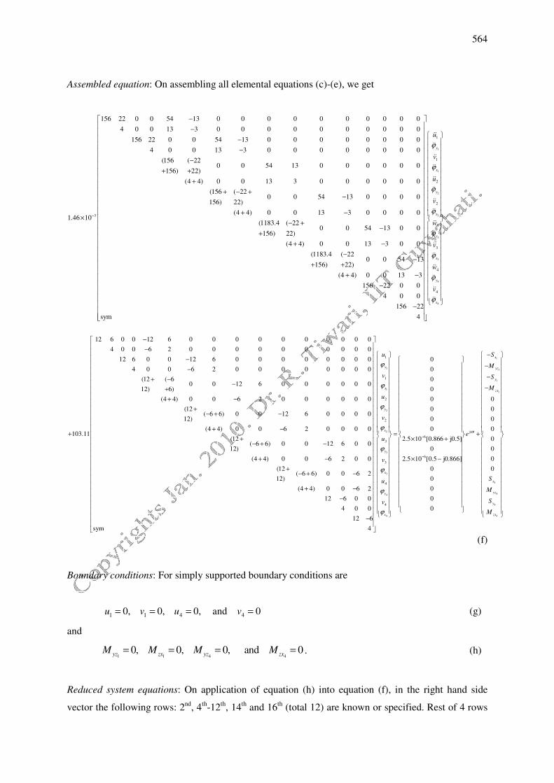
564

Assembled equation: On assembling all elemental equations (c)-(e), we get

3

156 22 0 0 54 13 0 0 0 0 0 0 0 0 0 0

4 0 0 13 3 0 0 0 0 0 0 0 0 0 0

156 22 0 0 54 13 0 0 0 0 0 0 0 0

4 0 0 13 3 0 0 0 0 0 0 0 0

(156 ( 220 0 54 13 0 0 0 0 0 0

156) 22)

(4 4) 0 0 13 3 0 0 0 0 0 0

(156 ( 220 0 54 13 0 0 0 0

156) 22)

(4 4) 0 0 13 3 0 0 0 01.46 10

(1183.4 ( 220 0 54 13 0 0

156) 22)

−

−

−

−

−

−

+ +

+

+ − +−

+ −×

− +−

+

1

1

2

2

3

3

4

1

1

2

2

3

3

4

(4 4) 0 0 13 3 0 0

(1183.4 ( 220 0 54 13

156) 22)

(4 4) 0 0 13 3

156 22 0 0

4 0 0

156 22

sym 4

y

x

y

x

y

x

y

u

v

u

v

w

v

w

ϕ

ϕ

ϕ

ϕ

ϕ

ϕ

ϕ

+ − − −

+ +

+ − − −

��

��

��

��

��

��

��

��

��

��

��

��

��

��

�

4

4

x

v

ϕ

�

��

12 6 0 0 12 6 0 0 0 0 0 0 0 0 0 0

4 0 0 6 2 0 0 0 0 0 0 0 0 0 0

12 6 0 0 12 6 0 0 0 0 0 0 0 0

4 0 0 6 2 0 0 0 0 0 0 0 0

(12 ( 60 0 12 6 0 0 0 0 0 0

12) 6)

(4 4) 0 0 6 2 0 0 0 0 0 0

(12( 6 6) 0 0 12 6 0 0 0 0

12)

(4 4) 0 0 6 2 0 0 0 0103.11

(12( 6 6) 0 0 12 6 0 0

12)

(4 4) 0 0 6 2 0 0

(12( 6 6) 0 0

12)

−

−

−

−

+ −−

+

+ −

+− + −

+ −+

+− + −

+ −

+− + −

1

1

2

2

3

3

4

4

1

1

2

2

3

3

4

4

0

0

0

0

0

0

0

0

2.5 10

6 2

(4 4) 0 0 6 2

12 6 0 0

4 0 0

12 6

sym 4

y

x

y

x

y

x

y

x

u

v

u

v

u

v

u

v

ϕ

ϕ

ϕ

ϕ

ϕ

ϕ

ϕ

ϕ

= ×

+ − − −

1

1

1

1

4

4

4

4

j

6

6

0

0

0

0

[0.866 j0.5] 0

0 0

2.5 10 [0.5 j0.866] 0

0 0

0

0

0

0

x

yz

y

zx

t

x

yz

y

zx

S

M

S

M

e

S

M

S

M

ω

−

−

−

− − −

+ +

× −

(f)

Boundary conditions: For simply supported boundary conditions are

1 1 4 40, 0, 0, and 0u v u v= = = = (g)

and

1 1 4 40, 0, 0, and 0

yz zx yz zxM M M M= = = = . (h)

Reduced system equations: On application of equation (h) into equation (f), in the right hand side

vector the following rows: 2nd

, 4th

-12th, 14

th and 16

th (total 12) are known or specified. Rest of 4 rows

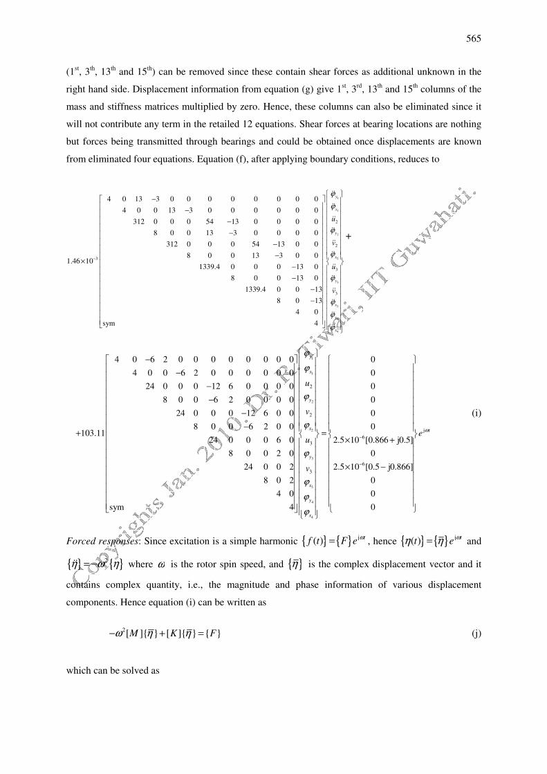
565

(1st, 3

th, 13

th and 15

th) can be removed since these contain shear forces as additional unknown in the

right hand side. Displacement information from equation (g) give 1st, 3

rd, 13

th and 15

th columns of the

mass and stiffness matrices multiplied by zero. Hence, these columns can also be eliminated since it

will not contribute any term in the retailed 12 equations. Shear forces at bearing locations are nothing

but forces being transmitted through bearings and could be obtained once displacements are known

from eliminated four equations. Equation (f), after applying boundary conditions, reduces to

1

1

2

2

2

2

3

3

4 0 13 3 0 0 0 0 0 0 0 0

4 0 0 13 3 0 0 0 0 0 0

312 0 0 0 54 13 0 0 0 0

8 0 0 13 3 0 0 0 0

312 0 0 0 54 13 0 0

8 0 0 13 3 0 01.46 10

1339.4 0 0 0 13 0

8 0 0 13 0

1339.4 0 0 13

8 0 13

4 0

sym 4

y

x

y

x

y

u

v

u

ϕ

ϕ

ϕ

ϕ

ϕ

−

− − −

− −

− × −

−

− −

��

��

��

��

��

��

��

��3

3

4

4

3

x

y

x

v

ϕ

ϕ

ϕ

��

��

��

��

+

1

1

2

2

3

3

4

4

2

2

3

3

4 0 6 2 0 0 0 0 0 0 0 0

4 0 0 6 2 0 0 0 0 0 0

24 0 0 0 12 6 0 0 0 0

8 0 0 6 2 0 0 0 0

24 0 0 0 12 6 0 0

8 0 0 6 2 0 0103.11

24 0 0 0 6 0

8 0 0 2 0

24 0 0 2

8 0 2

4 0

sym 4

y

x

y

x

y

x

y

x

u

v

u

v

ϕ

ϕ

ϕ

ϕ

ϕ

ϕ

ϕ

ϕ

−

− − − − − +

j

6

6

0

0

0

0

0

0

2.5 10 [0.866 j0.5]

0

2.5 10 [0.5 j0.866]

0

0

0

te

ω

−

−

=

× +

× −

(i)

Forced responses: Since excitation is a simple harmonic { } { } j( ) tf t F e

ω= , hence { } { } j( ) tt e

ωη η= and

{ } { }2η ω η= −�� where ω is the rotor spin speed, and { }η

is the complex displacement vector and it

contains complex quantity, i.e., the magnitude and phase information of various displacement

components. Hence equation (i) can be written as

2[ ]{ } [ ]{ } { }M K Fω η η− + = (j)

which can be solved as

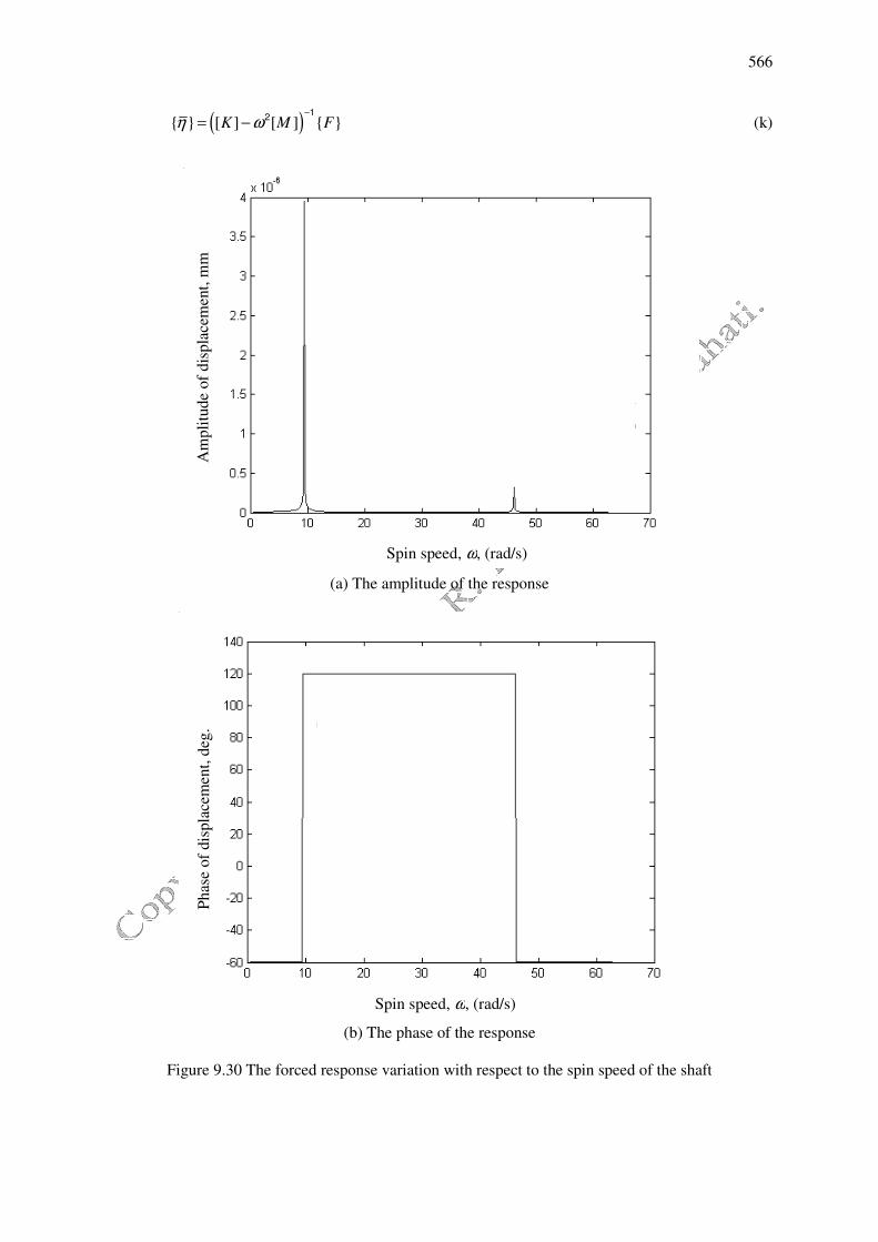
( ){ } [ ] [ ] { }K M Fη ω−

= −1

2

Figure 9.30 The forced response variation with respect to the spin speed of the shaft

Am

pli

tud

e of

dis

pla

cem

ent,

mm

P

has

e of

dis

pla

cem

ent,

deg

.

{ } [ ] [ ] { }K M F1

(a) The amplitude of the response

(b) The phase of the response

The forced response variation with respect to the spin speed of the shaft

Spin speed, ω, (rad/s)

Spin speed, ω, (rad/s)

566

(k)

The forced response variation with respect to the spin speed of the shaft

567

It should be noted that matrices [M] and [K] contain real quantities, whereas force vector {F} and

corresponding displacement vector { }η contain complex terms. The response (amplitudes and

phases) can be plotted with respect to shaft speeds. Figure 9.30 shows such typical plots. Critical

speeds could be observed at two places where amplitude of unbalance response has spikes, whereas in

the phase plot it is accompanied by change in phase of the order of 1800. We have done two plane

analysis for the present case, however, since as such there is no coupling in two planes hence still it

would be possible to obtain the unbalance response by considering a single plane motion only (in

vertical or horizontal plane).

9.5 Proportional Damping

The equation of motion for the shaft element with damping for free vibrations can be written as

( ) ( ) ( ) ( ) ( ) ( )[ ] { ( )} [ ] { ( )} [ ] { ( )} {0}e e e e e eM t C t K tη η η+ + =�� � (9.111)

where ( )[ ] e

M is the element mass matrix, ( )[ ] e

C is the element damping matrix, ( )[ ] e

K is the element

stiffness matrix, and ( ){ ( )} e

tη is the element vector of nodal degrees of freedom (dofs). The damping

matrix ( )[ ] e

C of the beam element can be expressed in terms of the element mass and stiffness

matrices as

( ) ( ) ( )

0 1[ ] [ ] [ ]e e eC a M a K= + (9.112)

where a0 and a1 are Rayleigh damping factors. The relation between the damping ratio, ζ , and the

natural frequency nfω in terms of a0 and a1 are given as (Clough and Penzien, 1993)

10

2 2

n

n

nf

n

nf

aa ωζ

ω= + (9.113)

where 0a and 1a are Rayleigh damping factors and this can be evaluated by the solution of a pair of

simultaneous equations, if damping ratios mζ and

nζ associated with two specific known frequencies

mnfω and nnfω . Writing equation (9.113) for each of these two cases and expressing them in the

matrix form leads to

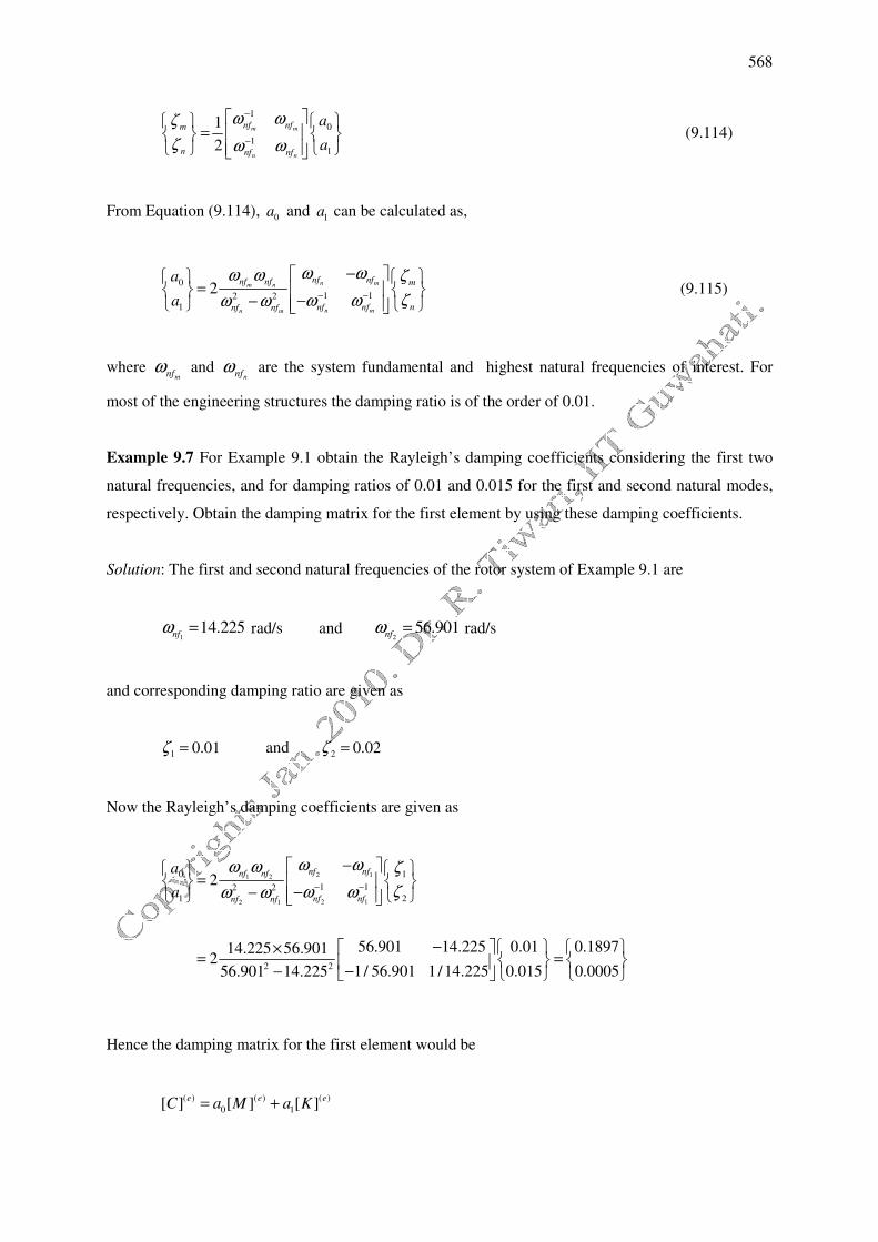
568

1

0

11

1

2

m m

n n

nf nfm

n nf nf

a

a

ω ωζ

ζ ω ω

−

−

=

(9.114)

From Equation (9.114), 0a and

1a can be calculated as,

0

1 12 2

1

2n mm n

n mn m

nf nfnf nf m

nnf nfnf nf

a

a

ω ωω ω ζ

ζω ωω ω − −

− =

−− (9.115)

where mnfω and

nnfω are the system fundamental and highest natural frequencies of interest. For

most of the engineering structures the damping ratio is of the order of 0.01.

Example 9.7 For Example 9.1 obtain the Rayleigh’s damping coefficients considering the first two

natural frequencies, and for damping ratios of 0.01 and 0.015 for the first and second natural modes,

respectively. Obtain the damping matrix for the first element by using these damping coefficients.

Solution: The first and second natural frequencies of the rotor system of Example 9.1 are

114.225

nfω = rad/s and

256.901

nfω = rad/s

and corresponding damping ratio are given as

1 0.01ζ = and

2 0.02ζ =

Now the Rayleigh’s damping coefficients are given as

2 11 2

2 12 1

0 1

1 12 2

1 2

2 2

2

56.901 14.225 0.01 0.189714.225 56.9012

1/ 56.901 1/14.225 0.015 0.000556.901 14.225

nf nfnf nf

nf nfnf nf

a

a

ω ωω ω ζ

ζω ωω ω − −

− =

−−

− ×= = −−

Hence the damping matrix for the first element would be

( ) ( ) ( )

0 1[ ] [ ] [ ]e e eC a M a K= +

569

( ) ( ) ( )

0 1

3

0 1

[ ] [ ] [ ]

156 22 54 13 12 6 12 6

4 13 3 4 6 21.46 10 103.11

156 22 12 6

sym 4 sym 4

e e eC a M a K

a a−

= +

− − − − = × × + × − −

0.623 0.296 0.565 0.286

0.296 0.194 0.286 0.096

0.565 0.286 0.623 0.296

0.286 0.096 0.296 0.1944

− − = − − −

−

It should be noted that the damping matrix is also remain symmetric. Determination of natural

frequencies (i.e., the eigen value problem formulation in the state space form) with damping in the

system would be dealt in subsequent chapter when we will consider the rotors mounted on fluid-film

bearings by using the FEM.

9.6 The Static and Dynamic Condensations

The static (or Guyan) and dynamic reduction methods are generally used to reduce certain degrees of

freedom in finite element equations. Similarly, we have expansion schemes to overcome the limitation

of number of measurements in practical rotors. The response is measured at only a limited number of

locations and over a limited frequency range; hence only a relatively small number of mode shape

vectors with a reduced number of elements are measured. Difficulty arises in comparing measured

experimental data with numerically generated data because of incomplete information. One way to

compare the data is to reduce the number of DOFs in the analytical model or expand the number of

DOFs from the limited measured DOFs. The most popular and the simplest method is the static

reduction introduced by Guyan (1965), which is accurate at low frequency range only. The static

method may be modified to reproduce the exact response of structure at any frequency. This is called

the dynamic reduction method and it is an extension to Guyan’s method. Paz (1984) used this method

in an iterative algorithm to save computational effort in calculating the eigensystem of a structure.

O’Callahan (1989) introduced a technique known as the Improved Reduction System (IRS) that is an

improvement on the static reduction method, and in fact provides a perturbation to the transformation

from the static case by including the inertia term as pseudo static forces. Friswell et al. (1994) gave an

iterative IRS method that converges to the same transformation as System Equivalent Reduction

Expansion Process (SEREP) (O’Callahan et al., 1989). The SEREP uses the computed eigenvectors to

produce the transformation between the master and slave coordinates. Kane and Torby (1991) gave a

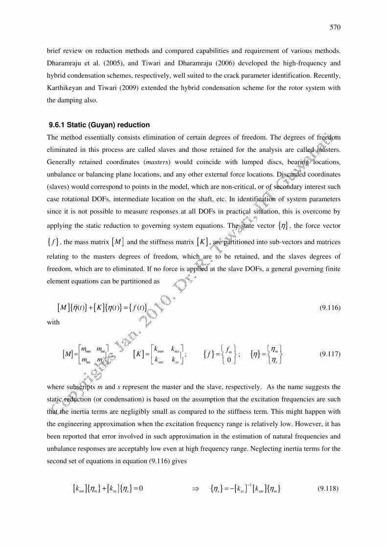
570

brief review on reduction methods and compared capabilities and requirement of various methods.

Dharamraju et al. (2005), and Tiwari and Dharamraju (2006) developed the high-frequency and

hybrid condensation schemes, respectively, well suited to the crack parameter identification. Recently,

Karthikeyan and Tiwari (2009) extended the hybrid condensation scheme for the rotor system with

the damping also.

9.6.1 Static (Guyan) reduction

The method essentially consists elimination of certain degrees of freedom. The degrees of freedom

eliminated in this process are called slaves and those retained for the analysis are called masters.

Generally retained coordinates (masters) would coincide with lumped discs, bearing locations,

unbalance or balancing plane locations, and any other external force locations. Discarded coordinates

(slaves) would correspond to points in the model, which are non-critical, or of secondary interest such

case rotational DOFs, intermediate location on the shaft, etc. In identification of system parameters

since it is not possible to measure responses at all DOFs in practical situation, this is overcome by

applying the static reduction to governing system equations. The state vector { }η , the force vector

{ }f , the mass matrix [ ]M and the stiffness matrix [ ]K , are partitioned into sub-vectors and matrices

relating to the masters degrees of freedom, which are to be retained, and the slaves degrees of

freedom, which are to eliminated. If no force is applied at the slave DOFs, a general governing finite

element equations can be partitioned as

[ ]{ } [ ]{ } { }( ) ( ) ( )M t K t f tη η+ =�� (9.116)

with

[ ] mm ms

sm ss

m mM

m m

=

; [ ] mm ms

sm ss

k kK

k k

=

; { }0

mff

=

; { } m

s

ηη

η

=

(9.117)

where subscripts m and s represent the master and the slave, respectively. As the name suggests the

static reduction (or condensation) is based on the assumption that the excitation frequencies are such

that the inertia terms are negligibly small as compared to the stiffness term. This might happen with

the engineering approximation when the excitation frequency range is relatively low. However, it has

been reported that error involved in such approximation in the estimation of natural frequencies and

unbalance responses are acceptably low even at high frequency range. Neglecting inertia terms for the

second set of equations in equation (9.116) gives

[ ]{ } [ ]{ } 0sm m ss sk kη η+ = { } [ ] [ ]{ }1

s ss sm m

k kη η−

⇒ = − (9.118)

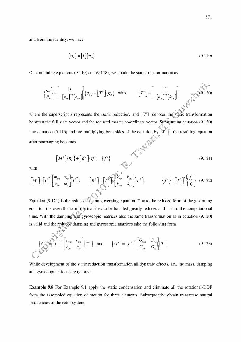
571

and from the identity, we have

{ } [ ]{ }m mIη η= (9.119)

On combining equations (9.119) and (9.118), we obtain the static transformation as

[ ] [ ]{ } { }1

[ ]m s

m m

s ss sm

IT

k k

ηη η

η −

= = −

with [ ] [ ]

1

[ ]s

ss sm

IT

k k−

= −

(9.120)

where the superscript s represents the static reduction, and [Ts] denotes the static transformation

between the full state vector and the reduced master co-ordinate vector. Substituting equation (9.120)

into equation (9.116) and pre-multiplying both sides of the equation by T

sT the resulting equation

after rearranging becomes

{ } { } { }s s s

m mM K fη η + = �� (9.121)

with

T mm mss s s

sm ss

m mM T T

m m

=

;

T mm mss s s

sm ss

k kK T T

k k

=

; { }

0

Ts s mff T

=

(9.122)

Equation (9.121) is the reduced system governing equation. Due to the reduced form of the governing

equation the overall size of the matrices to be handled greatly reduces and in turn the computational

time. With the damping and gyroscopic matrices also the same transformation as in equation (9.120)

is valid and the reduced damping and gyroscopic matrices take the following form

T mm mss s s

sm ss

c cC T T

c c

=

and

T mm mss s s

sm ss

G GG T T

G G

=

(9.123)

While development of the static reduction transformation all dynamic effects, i.e., the mass, damping

and gyroscopic effects are ignored.

Example 9.8 For Example 9.1 apply the static condensation and eliminate all the rotational-DOF

from the assembled equation of motion for three elements. Subsequently, obtain transverse natural

frequencies of the rotor system.

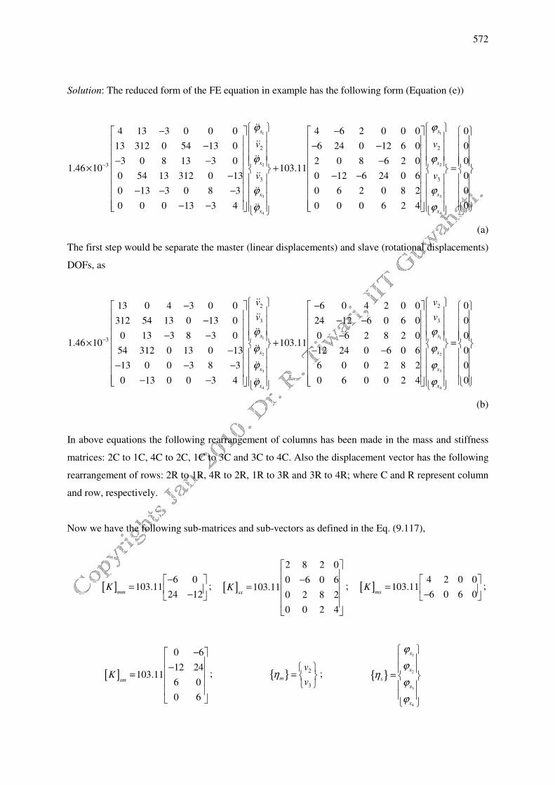
572

Solution: The reduced form of the FE equation in example has the following form (Equation (e))

1

2

3

4

2

3

3

4 13 3 0 0 0 4 6 2 0 0 0

13 312 0 54 13 0 6 24 0 12 6 0

3 0 8 13 3 0 2 0 8 6 2 01.46 10 103.11

0 54 13 312 0 13 0 12 6 24 0 6

0 13 3 0 8 3 0 6 2 0 8 2

0 0 0 13 3 4 0 0 0 6 2 4

x

x

x

x

v

v

ϕ

ϕ

ϕ

ϕ

−

− − − − − − − −

× + − − −

− − −

− −

��

��

��

��

��

��

1

2

3

4

2

3

0

0

0

0

0

0

x

x

x

x

v

v

ϕ

ϕ

ϕ

ϕ

=

(a)

The first step would be separate the master (linear displacements) and slave (rotational displacements)

DOFs, as

1

2

3

4

2

3

3

13 0 4 3 0 0 6 0 4 2 0 0

312 54 13 0 13 0 24 12 6 0 6 0

0 13 3 8 3 0 0 6 2 8 2 01.46 10 103.11

54 312 0 13 0 13 12 24 0 6 0 6

13 0 0 3 8 3 6 0 0 2 8 2

0 13 0 0 3 4 0 6 0 0 2 4

x

x

x

x

v

v

ϕ

ϕ

ϕ

ϕ

−

− − − − − − − −

× + − − −

− − −

− −

��

��

��

��

��

��

1

2

3

4

2

3

0

0

0

0

0

0

x

x

x

x

v

v

ϕ

ϕ

ϕ

ϕ

=

(b)

In above equations the following rearrangement of columns has been made in the mass and stiffness

matrices: 2C to 1C, 4C to 2C, 1C to 3C and 3C to 4C. Also the displacement vector has the following

rearrangement of rows: 2R to 1R, 4R to 2R, 1R to 3R and 3R to 4R; where C and R represent column

and row, respectively.

Now we have the following sub-matrices and sub-vectors as defined in the Eq. (9.117),

[ ]6 0

103.1124 12mm

K−

= − ; [ ]

2 8 2 0

0 6 0 6103.11

0 2 8 2

0 0 2 4

ssK

− =

;

[ ]4 2 0 0

103.116 0 6 0ms

K

= − ;

[ ]

0 6

12 24103.11

6 0

0 6

smK

− − =

; { } 2

3

m

v

vη

=

; { }

1

2

3

4

x

x

s

x

x

ϕ

ϕη

ϕ

ϕ

=

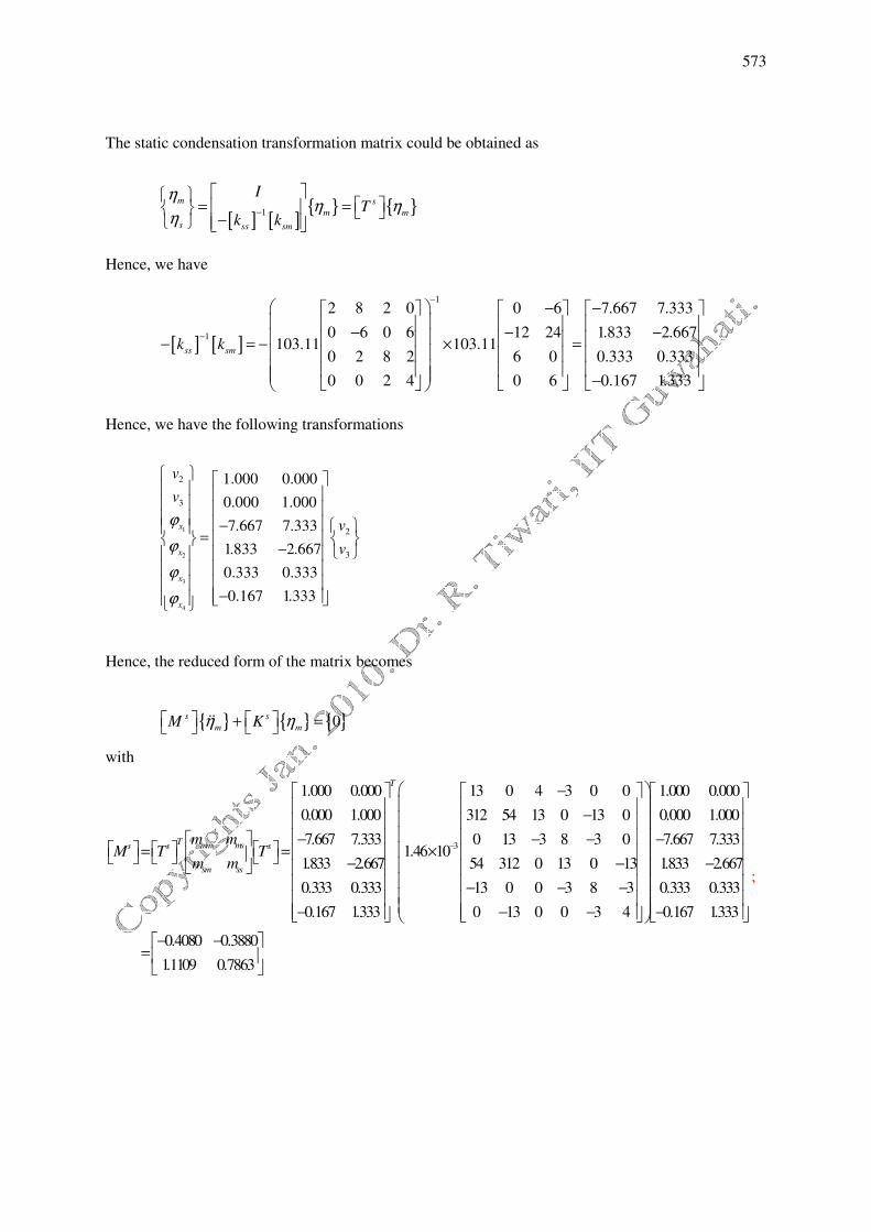
573

The static condensation transformation matrix could be obtained as

[ ] [ ]{ } { }1

m s

m m

s ss sm

IT

k k

ηη η

η −

= = −

Hence, we have

[ ] [ ]

1

1

2 8 2 0 0 6 7.667 7.333

0 6 0 6 12 24 1.833 2.667103.11 103.11

0 2 8 2 6 0 0.333 0.333

0 0 2 4 0 6 0.167 1.333

ss smk k

−

−

− − − − − − = − × = −

Hence, we have the following transformations

1

2

3

4

2

3

2

3

1.000 0.000

0.000 1.000

7.667 7.333

1.833 2.667

0.333 0.333

0.167 1.333

x

x

x

x

v

v

v

v

ϕ

ϕ

ϕ

ϕ

−

= −

−

Hence, the reduced form of the matrix becomes

{ } { } { }0s s

m mM Kη η + = ��

with

3

1.000 0.000 13 0 4 3 0 0

0.000 1.000 312 54 13 0 13 0

7.667 7.333 0 13 3 8 3 01.46 10

1.833 2.667 54 312 0 13 0 13

0.333 0.333 13 0 0 3 8 3

0.167 1.333 0 13 0 0 3 4

T

T mm mss s s

sm ss

m mM T T

m m

−

− − − − −

= = × − − − − − − − −

1.000 0.000

0.000 1.000

7.667 7.333

1.833 2.667

0.333 0.333

0.167 1.333

0.4080 0.3880

1.1109 0.7863

−

− −

− − =

;

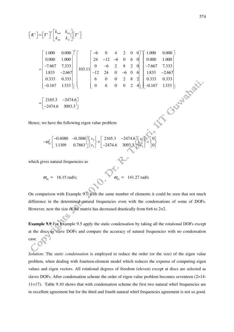
574

1.000 0.000 6 0 4 2 0 0

0.000 1.000 24 12 6 0 6 0

7.667 7.333 0 6 2 8 2 0103.11

1.833 2.667 12 24 0 6 0 6

0.333 0.333 6 0 0 2 8 2

0.167 1.333 0 6 0 0 2 4

T mm mss s s

sm ss

T

k kK T T

k k

=

− − − − −

= − − −

−

1.000 0.000

0.000 1.000

7.667 7.333

1.833 2.667

0.333 0.333

0.167 1.333

2165.3 2474.6

2474.6 3093.3

−

−

−

− = −

Hence, we have the following eigen value problem

2 22

3 3

0.4080 0.3880 2165.3 2474.6 0

1.1109 0.7863 2474.6 3093.3 0nf

v v

v vω

− − − − + = −

which gives natural frequencies as

1nf

ω = 16.15 rad/s; 1nf

ω = 141.27 rad/s

On comparison with Example 9.1 with the same number of elements it could be seen that not much

difference in the determined natural frequencies even with the condensations of some of DOFs.

However, now the size of the matrix has decreased drastically from 6×6 to 2×2.

Example 9.9 For Example 9.5 apply the static condensation by taking all the rotational DOFs except

at the discs as slave DOFs and compare the accuracy of natural frequencies with no condensation

case.

Solution: The static condensation is employed to reduce the order (or the size) of the eigen value

problem, when dealing with fourteen-element model which reduces the expense of computing eigen

values and eigen vectors. All rotational degrees of freedom (eleven) except at discs are selected as

slaves DOFs. After condensation scheme the order of eigen value problem becomes seventeen (2×14-

11=17). Table 9.10 shows that with condensation scheme the first two natural whirl frequencies are

in excellent agreement but for the third and fourth natural whirl frequencies agreement is not so good.

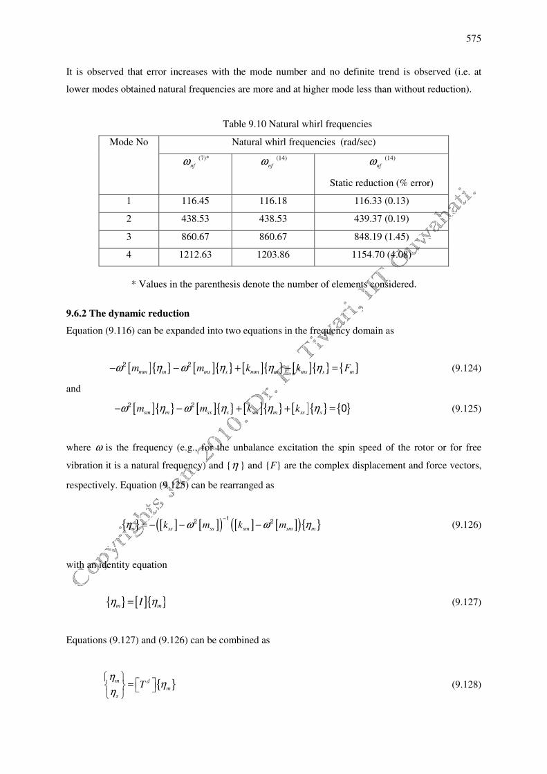
575

It is observed that error increases with the mode number and no definite trend is observed (i.e. at

lower modes obtained natural frequencies are more and at higher mode less than without reduction).

Table 9.10 Natural whirl frequencies

Mode No Natural whirl frequencies (rad/sec)

nfω (7)*

nf

ω (14)

nfω (14)

Static reduction (% error)

1 116.45 116.18 116.33 (0.13)

2 438.53 438.53 439.37 (0.19)

3 860.67 860.67 848.19 (1.45)

4 1212.63 1203.86 1154.70 (4.08)

* Values in the parenthesis denote the number of elements considered.

9.6.2 The dynamic reduction

Equation (9.116) can be expanded into two equations in the frequency domain as

[ ]{ } [ ]{ } [ ]{ } [ ]{ } { }mm m ms s mm m ms s mm m k k Fω η ω η η η− − + + =2 2 (9.124)

and

[ ]{ } [ ]{ } [ ]{ } [ ]{ } { }sm m ss s sm m ss sm m k kω η ω η η η− − + + =2 2 0 (9.125)

where ω is the frequency (e.g., for the unbalance excitation the spin speed of the rotor or for free

vibration it is a natural frequency) and {η } and {F} are the complex displacement and force vectors,

respectively. Equation (9.125) can be rearranged as

{ } [ ] [ ]( ) [ ] [ ]( ){ }s ss ss sm sm mk m k mη ω ω η−

= − − −1

2 2 (9.126)

with an identity equation

{ } [ ]{ }m mIη η= (9.127)

Equations (9.127) and (9.126) can be combined as

{ }m d

m

s

Tη

ηη

=

(9.128)

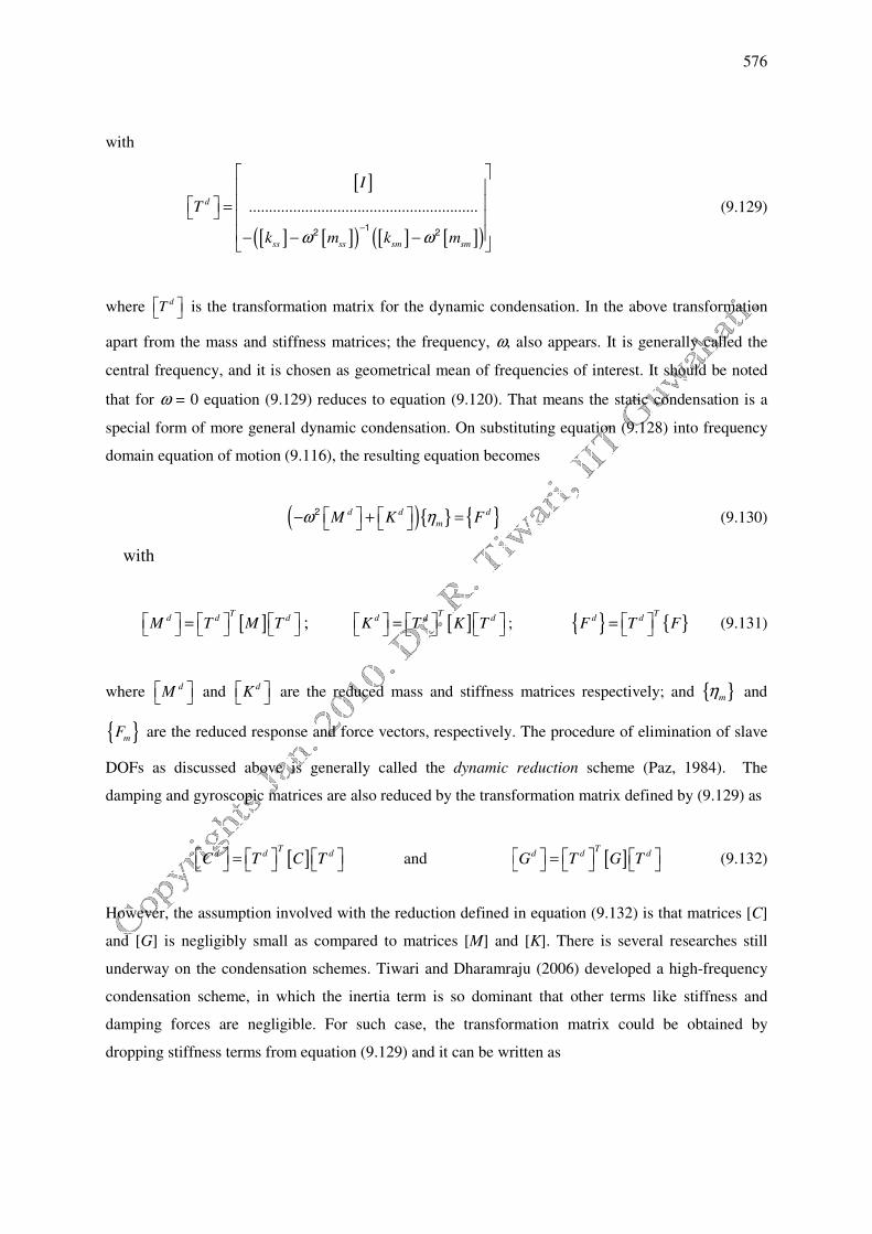
576

with

[ ]

[ ] [ ]( ) [ ] [ ]( )

.........................................................d

ss ss sm sm

I

T

k m k mω ω−

= − − −

12 2

(9.129)

where dT is the transformation matrix for the dynamic condensation. In the above transformation

apart from the mass and stiffness matrices; the frequency, ω, also appears. It is generally called the

central frequency, and it is chosen as geometrical mean of frequencies of interest. It should be noted

that for ω = 0 equation (9.129) reduces to equation (9.120). That means the static condensation is a

special form of more general dynamic condensation. On substituting equation (9.128) into frequency

domain equation of motion (9.116), the resulting equation becomes

( ){ } { }d d d

mM K Fω η − + =

2 (9.130)

with

[ ]T

d d dM T M T = ; [ ]

Td d d

K T K T = ; { } { }T

d dF T F = (9.131)

where dM and dK are the reduced mass and stiffness matrices respectively; and { }mη and

{ }mF are the reduced response and force vectors, respectively. The procedure of elimination of slave

DOFs as discussed above is generally called the dynamic reduction scheme (Paz, 1984). The

damping and gyroscopic matrices are also reduced by the transformation matrix defined by (9.129) as

[ ]T

d d dC T C T = and [ ]

Td d d

G T G T = (9.132)

However, the assumption involved with the reduction defined in equation (9.132) is that matrices [C]

and [G] is negligibly small as compared to matrices [M] and [K]. There is several researches still

underway on the condensation schemes. Tiwari and Dharamraju (2006) developed a high-frequency

condensation scheme, in which the inertia term is so dominant that other terms like stiffness and

damping forces are negligible. For such case, the transformation matrix could be obtained by

dropping stiffness terms from equation (9.129) and it can be written as

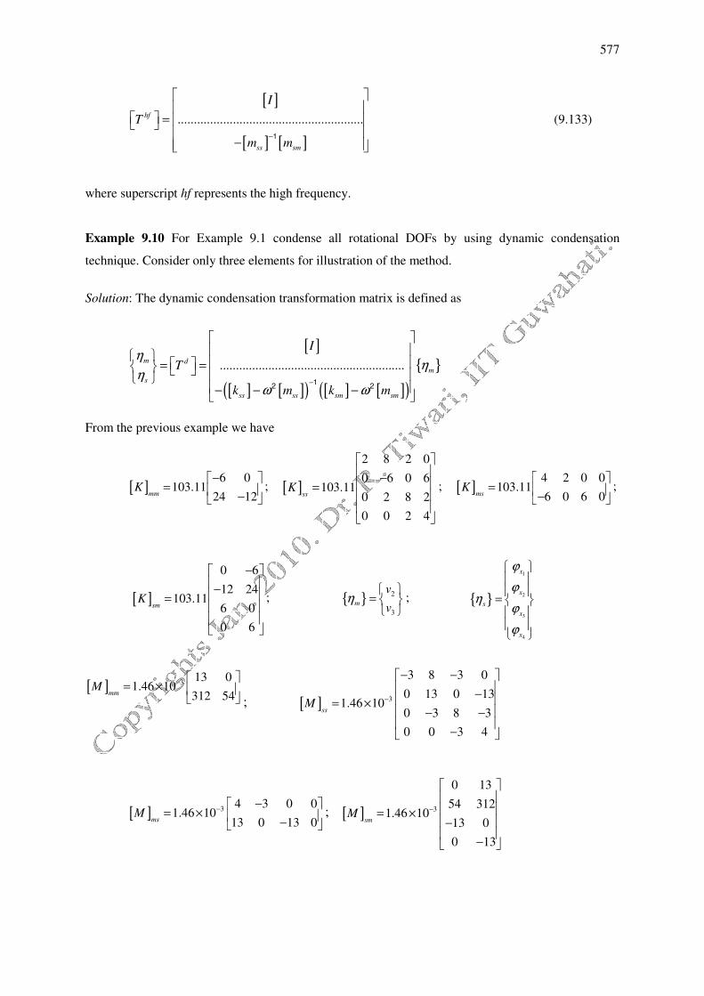
577

[ ]

[ ] [ ]

.........................................................hf

ss sm

I

T

m m−

=

− 1

(9.133)

where superscript hf represents the high frequency.

Example 9.10 For Example 9.1 condense all rotational DOFs by using dynamic condensation

technique. Consider only three elements for illustration of the method.

Solution: The dynamic condensation transformation matrix is defined as

[ ]

[ ] [ ]( ) [ ] [ ]( ){ }.........................................................

m d

m

s

ss ss sm sm

I

T

k m k m

ηη

ηω ω

−

= = − − −

12 2

From the previous example we have

[ ]6 0

103.1124 12mm

K−

= − ; [ ]

2 8 2 0

0 6 0 6103.11

0 2 8 2

0 0 2 4

ssK

− =

;

[ ]4 2 0 0

103.116 0 6 0ms

K

= − ;

[ ]

0 6

12 24103.11

6 0

0 6

smK

− − =

; { } 2

3

m

v

vη

=

; { }

1

2

3

4

x

x

s

x

x

ϕ

ϕη

ϕ

ϕ

=

[ ] 313 0

1.46 10312 54mm

M−

= × ; [ ] 3

3 8 3 0

0 13 0 131.46 10

0 3 8 3

0 0 3 4

ssM

−

− − − = × − −

−

[ ] 34 3 0 0

1.46 1013 0 13 0ms

M− −

= × − ; [ ] 3

0 13

54 3121.46 10

13 0

0 13

smM

−

= × −

−

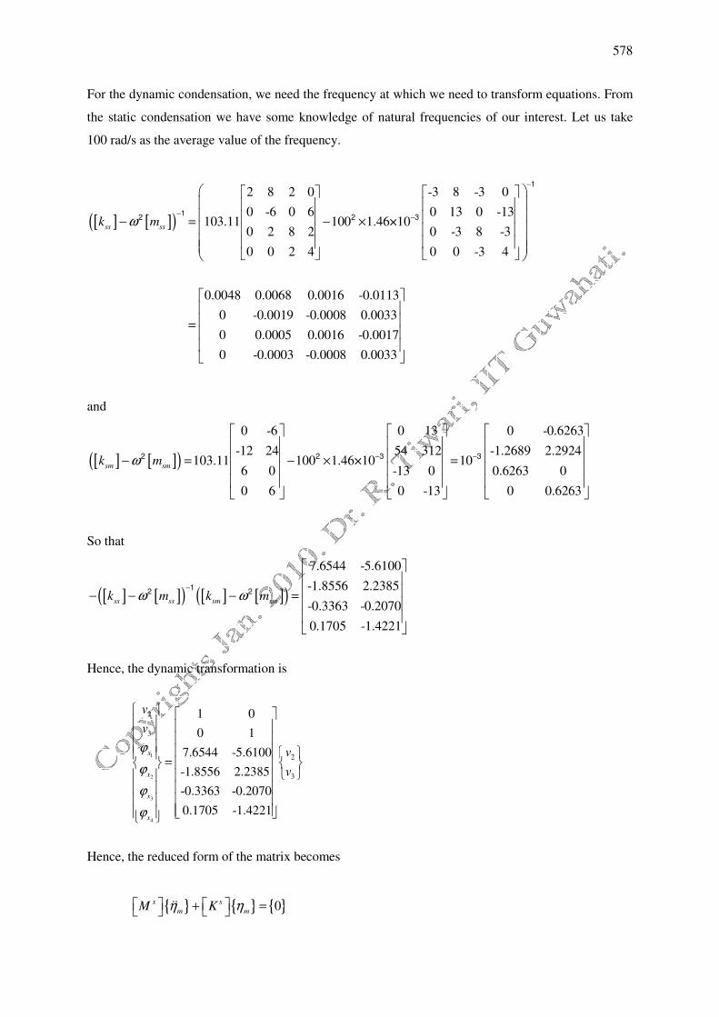
578

For the dynamic condensation, we need the frequency at which we need to transform equations. From

the static condensation we have some knowledge of natural frequencies of our interest. Let us take

100 rad/s as the average value of the frequency.

[ ] [ ]( )

2 8 2 0 -3 8 -3 0

0 -6 0 6 0 13 0 -13103.11 100 1.46×10

0 2 8 2 0 -3 8 -3

0 0 2 4 0 0 -3 4

0.0048 0.0068 0.0016 -0.0113

0 -0.0019 -0.0008 0.0033

0 0.0005 0.0016 -0.0017

0 -0.0003 -0.0008 0.00

ss ssk mω

−

−−

− = − ×

=

1

12 2 3

33

and

[ ] [ ]( )

0 -6 0 13 0 -0.6263

-12 24 54 312 -1.2689 2.2924103.11 100 1.46×10 10

6 0 -13 0 0.6263 0

0 6 0 -13 0 0.6263

sm smk mω − −

− = − × =

2 2 3 3

So that

[ ] [ ]( ) [ ] [ ]( )

7.6544 -5.6100

-1.8556 2.2385

-0.3363 -0.2070

0.1705 -1.4221

ss ss sm smk m k mω ω

−

− − − =

12 2

Hence, the dynamic transformation is

1

2

3

4

2

3

2

3

1 0

0 1

7.6544 -5.6100

-1.8556 2.2385

-0.3363 -0.2070

0.1705 -1.4221

x

x

x

x

v

v

v

v

ϕ

ϕ

ϕ

ϕ

=

Hence, the reduced form of the matrix becomes

{ } { } { }0s s

m mM Kη η + = ��

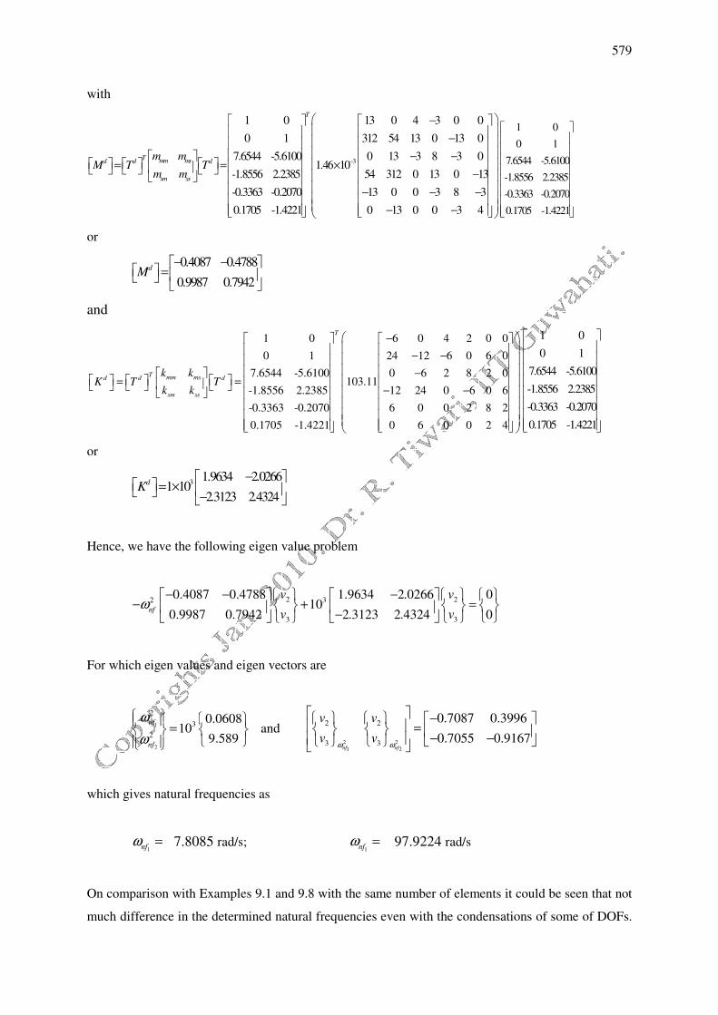
579

with

3

1 0 13 0 4 3 0 0

0 1 312 54 13 0 13 0

7.6544 -5.6100 0 13 3 8 3 01.46 10

-1.8556 2.2385 54 312 0 13 0 13

-0.3363 -0.2070 13 0 0 3 8 3

0.1705 -1.4221 0 13 0 0 3 4

T

T mm msd d d

sm ss

m mM T T

m m

−

− − − −

= = × − − − −

− −

1 0

0 1

7.6544 -5.6100

-1.8556 2.2385

-0.3363 -0.2070

0.1705 -1.4221

or

0.4087 0.4788

0.9987 0.7942

dM− −

=

and

1 0 6 0 4 2 0 0

0 1 24 12 6 0 6 0

7.6544 -5.6100 0 6 2 8 2 0103.11

-1.8556 2.2385 12 24 0 6 0 6

-0.3363 -0.2070 6 0 0 2 8 2

0.1705 -1.4221 0 6 0 0 2 4

T

T mm msd d d

sm ss

k kK T T

k k

− − − −

= = − −

1 0

0 1

7.6544 -5.6100

-1.8556 2.2385

-0.3363 -0.2070

0.1705 -1.4221

or

31.9634 2.0266

1 102.3123 2.4324

dK−

= × −

Hence, we have the following eigen value problem

2 22 3

3 3

0.4087 0.4788 1.9634 2.0266 010

0.9987 0.7942 2.3123 2.4324 0nf

v v

v vω

− − − − + = −

For which eigen values and eigen vectors are

1

2

2

3

2

0.060810

9.589

nf

nf

ω

ω

=

and 2 2

1 2

2 2

3 3

0.7087 0.3996

0.7055 0.9167nf nf

v v

v vω ω

− = − −

which gives natural frequencies as

1nf

ω = 7.8085 rad/s; 1nf

ω = 97.9224 rad/s

On comparison with Examples 9.1 and 9.8 with the same number of elements it could be seen that not

much difference in the determined natural frequencies even with the condensations of some of DOFs.

580

However, now the size of the matrix has decreased drastically from 6×6 to 2×2. The difference

between the condensed and non-condensed cases would be very less when we will have very large

DOFs system. The present example, in fact illustrate the method but not the potential of the dynamic

condensation as such.

Concluding Remarks

To brief, in the present chapter we considered transverse vibration of continuous system for some

simple boundary conditions. Natural frequencies and mode shapes are summarised for various

boundary conditions. The main focus of the present chapter is to analyse the free and forced vibrations

by using the finite element method. Various boundary conditions like the simply supported, over-

hanged, intermediate supports, etc. have been illustrated through examples. The purpose of the

examples are to have clarity of intermediate steps involved in the formulation of the elemental and

assembled governing equations, application of boundary conditions, and extraction of modal

parameters and forced response information. The static and dynamic condensation schemes are

described in detailed, which are used to reduce the size of matrices to be handled for final solution of

either the eigen value problem or to obtained the forced response. The forced response of simple rotor

systems are obtained for most common type of excitation, i.e., unbalances. However, the analysis can

be easily extended for other periodic forces by using the Fourier analysis, as any periodic force can be

written as the sine and cosine series form. Fourier series will be dealt in more detail in subsequent

chapters. In next chapter, we will continue with the finite element analysis of rotors by including

some higher effects like gyroscopic effects and the shear deformation; which are predominant for at

high spin speeds and thick shafts, respectively.

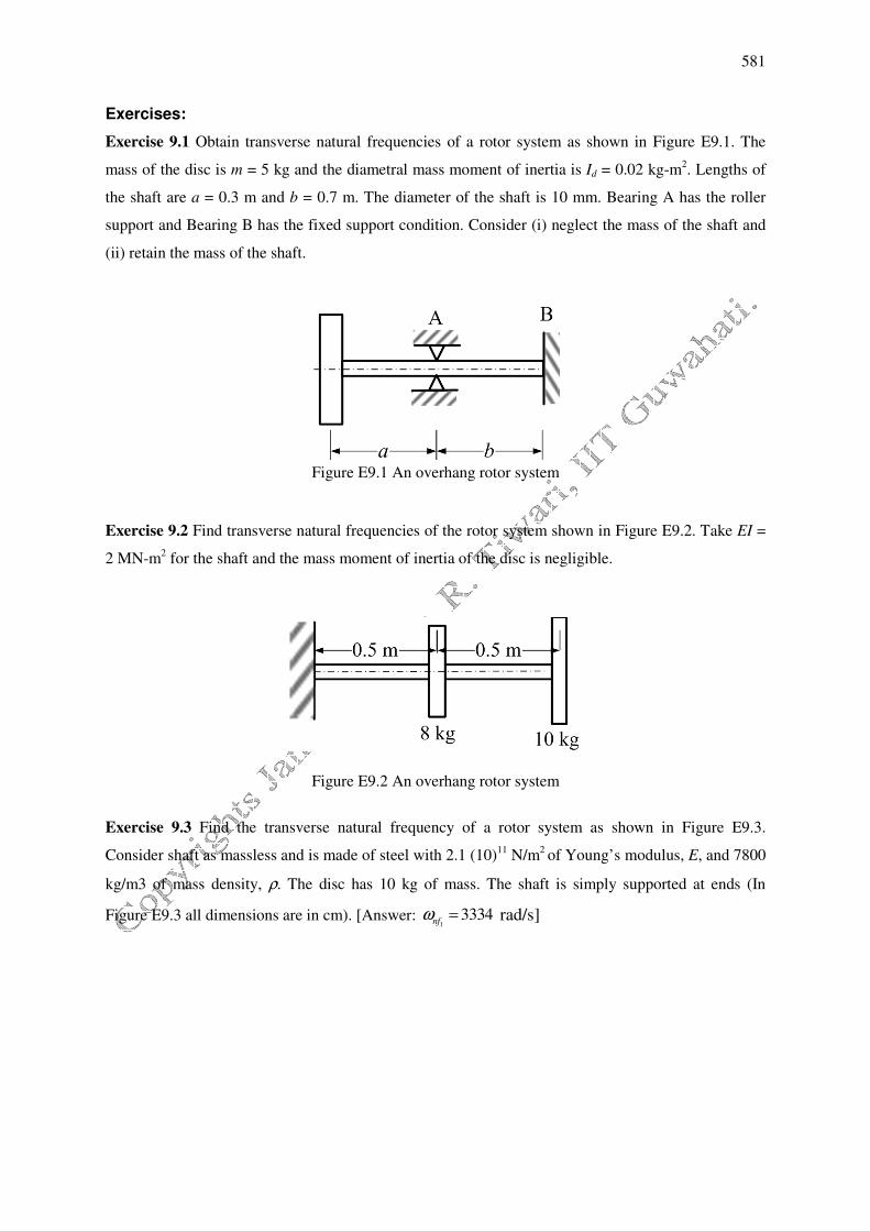
581

Exercises:

Exercise 9.1 Obtain transverse natural frequencies of a rotor system as shown in Figure E9.1. The

mass of the disc is m = 5 kg and the diametral mass moment of inertia is Id = 0.02 kg-m2. Lengths of

the shaft are a = 0.3 m and b = 0.7 m. The diameter of the shaft is 10 mm. Bearing A has the roller

support and Bearing B has the fixed support condition. Consider (i) neglect the mass of the shaft and

(ii) retain the mass of the shaft.

Figure E9.1 An overhang rotor system

Exercise 9.2 Find transverse natural frequencies of the rotor system shown in Figure E9.2. Take EI =

2 MN-m2 for the shaft and the mass moment of inertia of the disc is negligible.

Figure E9.2 An overhang rotor system

Exercise 9.3 Find the transverse natural frequency of a rotor system as shown in Figure E9.3.

Consider shaft as massless and is made of steel with 2.1 (10)11

N/m2 of Young’s modulus, E, and 7800

kg/m3 of mass density, ρ. The disc has 10 kg of mass. The shaft is simply supported at ends (In

Figure E9.3 all dimensions are in cm). [Answer: 1

3334nf

ω = rad/s]

582

Figure E9.3

Exercise 9.4 For exercises 9.1 to 9.3 plot the linear and angular displacements (with both amplitude

and phase) of discs with respect to the rotational speed of the rotor (take the rotational frequency of

the rotor minimum of 0.1 rad/s and maximum at least 5 rad/s above the second critical speed of the

rotor system). Assume imbalances of 20 gm-mm at one of the disc with 30-degree phase with some

shaft reference point. Check whether critical speeds are in agreement with the obtained by free

vibration analysis.

Exercise 9.5 Obtain the bending natural frequency of a rotor as shown in Figure E9.5. The rotor is

assumed to be fixed supported at one end. Take mass of the disc m = 2 kg and its diametral moment of

inertia 0.05dI = kg-m2. The shaft is assumed to be massless, and its length and diameter are 0.2 m

and 0.01 m, respectively. Take the Young’s modulus 112.1 10E = × N/m2 for the shaft material.

Figure E9.5

Exercise 9.6 For Exercise E9.2 when the left and right discs have respectively diametral mass

moment of inertias as .d

I =1

0 05 kg-m2 and .

dI =

20 06 kg-m

2, obtain the transverse natural

frequencies and mode shapes of the rotor system.

Exercise 9.7 Obtain transverse natural frequencies of a rotor system as shown in Figure E9.7. The

mass of the disc is 5m = kg and the diametral mass moment of inertia is Id = 0.02 kg-m2. Shaft lengths

are a = 0.3 m and b = 0.7 m, the diameter of the shaft is 10 mm and the modulus of elasticity of the

shaft is E = 2.1 × 1011

N/m2. Consider two different cases i.e. when bearing A is (i) a simple support

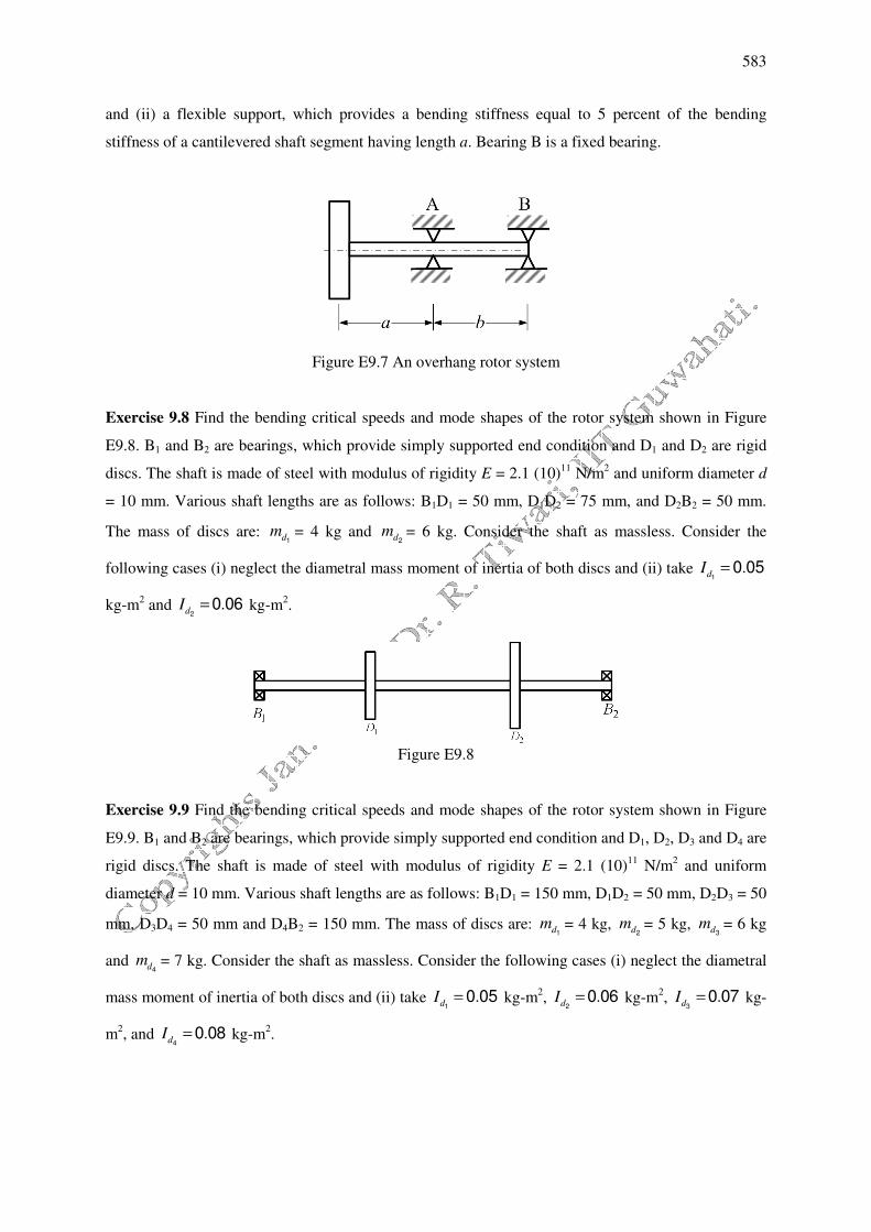
583

and (ii) a flexible support, which provides a bending stiffness equal to 5 percent of the bending

stiffness of a cantilevered shaft segment having length a. Bearing B is a fixed bearing.

Figure E9.7 An overhang rotor system

Exercise 9.8 Find the bending critical speeds and mode shapes of the rotor system shown in Figure

E9.8. B1 and B2 are bearings, which provide simply supported end condition and D1 and D2 are rigid

discs. The shaft is made of steel with modulus of rigidity E = 2.1 (10)11

N/m2 and uniform diameter d

= 10 mm. Various shaft lengths are as follows: B1D1 = 50 mm, D1D2 = 75 mm, and D2B2 = 50 mm.

The mass of discs are: dm

1= 4 kg and d

m2= 6 kg. Consider the shaft as massless. Consider the

following cases (i) neglect the diametral mass moment of inertia of both discs and (ii) take .d

I =1

0 05

kg-m2 and .

dI =

20 06 kg-m

2.

Figure E9.8

Exercise 9.9 Find the bending critical speeds and mode shapes of the rotor system shown in Figure

E9.9. B1 and B2 are bearings, which provide simply supported end condition and D1, D2, D3 and D4 are

rigid discs. The shaft is made of steel with modulus of rigidity E = 2.1 (10)11

N/m2 and uniform

diameter d = 10 mm. Various shaft lengths are as follows: B1D1 = 150 mm, D1D2 = 50 mm, D2D3 = 50

mm, D3D4 = 50 mm and D4B2 = 150 mm. The mass of discs are: dm

1= 4 kg, d

m2= 5 kg, d

m3= 6 kg

and dm

4= 7 kg. Consider the shaft as massless. Consider the following cases (i) neglect the diametral

mass moment of inertia of both discs and (ii) take .d

I =1

0 05 kg-m2, .

dI =

20 06 kg-m

2, .

dI =

30 07 kg-

m2, and .

dI =

40 08 kg-m

2.

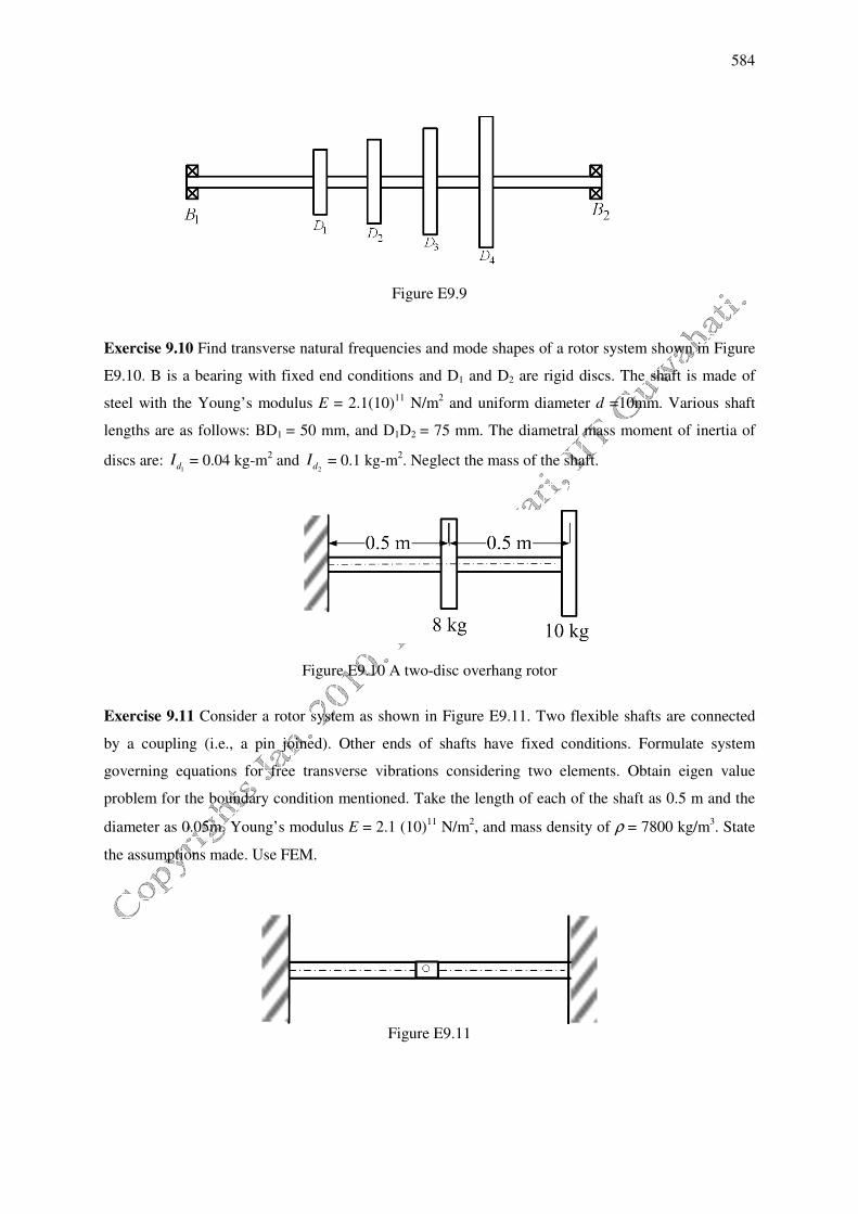
584

Figure E9.9

Exercise 9.10 Find transverse natural frequencies and mode shapes of a rotor system shown in Figure

E9.10. B is a bearing with fixed end conditions and D1 and D2 are rigid discs. The shaft is made of

steel with the Young’s modulus E = 2.1(10)11

N/m2 and uniform diameter d =10mm. Various shaft

lengths are as follows: BD1 = 50 mm, and D1D2 = 75 mm. The diametral mass moment of inertia of

discs are: 1d

I = 0.04 kg-m2 and

2dI = 0.1 kg-m

2. Neglect the mass of the shaft.

Figure E9.10 A two-disc overhang rotor

Exercise 9.11 Consider a rotor system as shown in Figure E9.11. Two flexible shafts are connected

by a coupling (i.e., a pin joined). Other ends of shafts have fixed conditions. Formulate system

governing equations for free transverse vibrations considering two elements. Obtain eigen value

problem for the boundary condition mentioned. Take the length of each of the shaft as 0.5 m and the

diameter as 0.05m. Young’s modulus E = 2.1 (10)11

N/m2, and mass density of ρ = 7800 kg/m

3. State

the assumptions made. Use FEM.

Figure E9.11

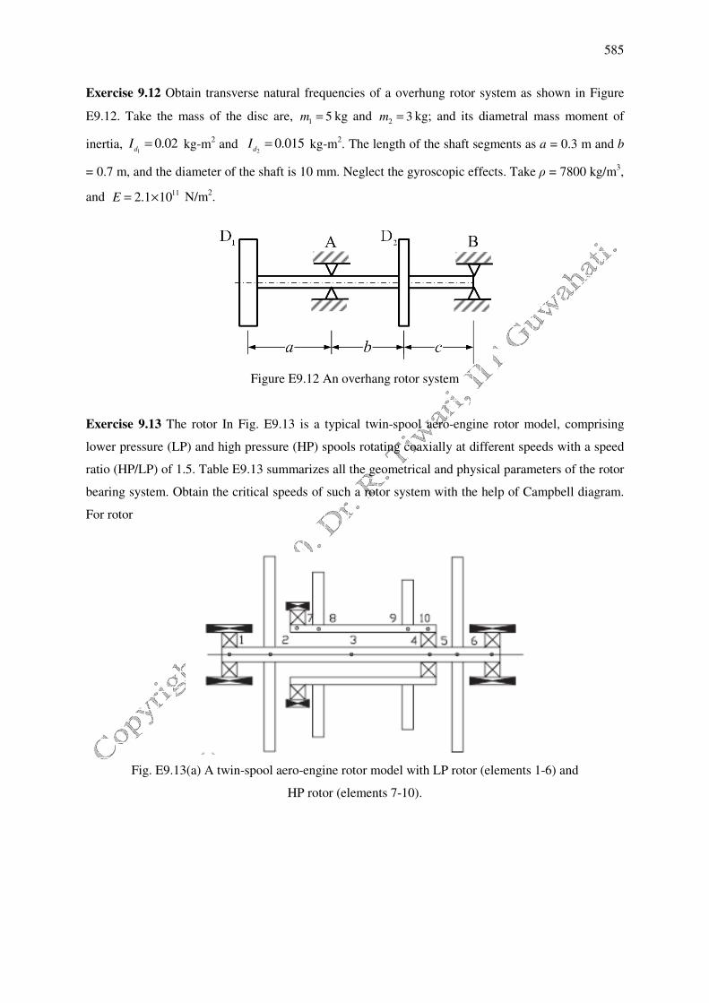
585

Exercise 9.12 Obtain transverse natural frequencies of a overhung rotor system as shown in Figure

E9.12. Take the mass of the disc are, 1 5m = kg and

2 3m = kg; and its diametral mass moment of

inertia, 1

0.02d

I = kg-m2 and

20.015

dI = kg-m

2. The length of the shaft segments as a = 0.3 m and b

= 0.7 m, and the diameter of the shaft is 10 mm. Neglect the gyroscopic effects. Take ρ = 7800 kg/m3,

and N/m2.

Figure E9.12 An overhang rotor system

Exercise 9.13 The rotor In Fig. E9.13 is a typical twin-spool aero-engine rotor model, comprising

lower pressure (LP) and high pressure (HP) spools rotating coaxially at different speeds with a speed

ratio (HP/LP) of 1.5. Table E9.13 summarizes all the geometrical and physical parameters of the rotor

bearing system. Obtain the critical speeds of such a rotor system with the help of Campbell diagram.

For rotor

Fig. E9.13(a) A twin-spool aero-engine rotor model with LP rotor (elements 1-6) and

HP rotor (elements 7-10).

112.1 10E = ×

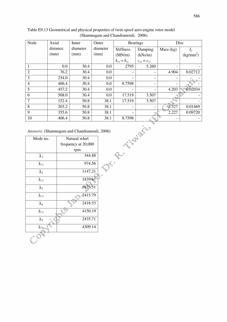
586

Table E9.13 Geometrical and physical properties of twin-spool aero-engine rotor model

(Shanmugam and Chandramouli, 2006)

Node Axial

distance

(mm)

Inner

diameter

(mm)

Outer

diameter

(mm)

Bearings Disc

Stiffness

(MN/m)

kxx = kyy

Damping

(kNs/m)

cxx = cyy

Mass (kg) Ip

(kg/mm2)

1 0.0 30.4 0.0 2795 5.260 - -

2 76.2 30.4 0.0 - - 4.904 0.02712

3 254.0 30.4 0.0 - - - -

4 406.4 30.4 0.0 8.7598 - - -

5 457.2 30.4 0.0 - - 4.203 0.02034

6 508.0 30.4 0.0 17.519 3.507 - -

7 152.4 50.8 38.1 17.519 3.507 - -

8 203.2 50.8 38.1 - - 3.327 0.01469

9 355.6 50.8 38.1 - - 2.227 0.09720

10 406.4 50.8 38.1 8.7598 - - -

Answers: (Shanmugam and Chandramouli, 2006)

Mode no. Natural whirl

frequency at 20,000

rpm

λ1 344.88

λ-1 974.56

λ2 1147.21

λ-2 1839.61

λ3 1623.51

λ-3 2415.79

λ4 2418.53

λ-4 4150.19

λ5 2435.71

λ-5 4309.14

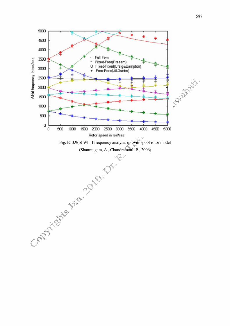
587

Fig. E13.9(b) Whirl frequency analysis of twin-spool rotor model

(Shanmugam, A., Chandramouli P., 2006)

588

References

Bickford, W.B., Greenhill, L.M., and Nelson, H.D., 1985, “A Conical Beam Finite Element for Rotor

Dynamics Analysis”, Transactions of the ASME, Journal of Vibration, Stress and Reliability in

Design, vol. 107, pp. 421-430.

Booker, J.F., and Ruhl, R.L., 1972, “A Finite Element Model for Distributed Parameter Turborotor

Systems”, ASME, Journal of Engineering for Industry, vol. 94, p. 126.

Booker, J.F., and Ruhl, R.L., 1986, “A Finite Element Model for Distributed Parameter Turborotor

Systems” , ASME, Journal of Vibration, Stress and Reliability in Design, vol. 108, pp. 177-181,

paper C432/142.

Chen, L.W., and Ku, D.M., 1991, “Finite Element Analysis of Natural Whirl Speeds of Rotating

Shafts”, Computers & Structures, vol. 40, pp. 741-747.

Chen, W.J., “A Note on Computational Rotor Dynamics”, Transactions of the ASME journal,

Journal of Vibration and Acoustics, vol.120, pp. 228-233.

Childs, D., Turbomachinery Rotordynamics, Phenomena, Modeling, and Analysis, John Wiley &

Sons, Inc., 1993.

Childs, D.W., and Graviss, K., 1982, “A Note on Critical-Speed Solutions for Finite Element Based

Rotor Models.” ASME, Journal of Mechanical Design, vol. 104, pp. 412-416.

Chong-Won Lee Vibration Analysis of Rotors, Kluwer Academic Publishers, 1993.

Clough R.W. and Penzien, J., Dynamics of Structures, McGraw-Hill, Inc 1993.

Cook, D., Malkus, D.W., and Plesha, M.E., Concepts and Applications of Finite Element Analysis,

John Wiley & Sons, Third Edition, 1989.

Craig Jr., R.R., Bampton, M.C.C., 1968, Coupling of substructures for dynamic analysis, AIAA

Journal, 6, 1313–1319.

Craig Jr., R. R., Chang, C-J., 1977, On the use of attachment modes in substructure coupling for

dynamic analysis, AIAA/ASME 18th Structures, Structural Dynamics and Material Conference,

San Diego, CA.

Crandall, H., S., Rotardynamics software, Rotating Machinery Dynamics (Proc.), 1992, pp. 3-21.

Den Hartog, J.,P., Mechanical Vibration, Dover Publications, Inc.,1985, pp. 262 – 263.

Diana, G., Massa, E., and Pizzigoni, 1975, “Finite Element Method for Computing Oil Whirl

Instability of A Rotating Shaft Supported by Elastic Bearings,” I. Mech. E., pp. 659-663.

Dimarganas, A.D., 1975, “A General Method for Stability Analysis of Rotating Shafts,” Inggenieur-

Archiv, vol.44, p. 126.

Dimentberg, F.M., 1961, Flexural Vibrations of Rotating Shafts, Butterworths, London.

Dutt, J.K., and Nakara, B.C., 1992, “Stability of Rotor Systems with Viscoelastic Supports,” Journal

of Sound and Vibration, vol.153, No.1, pp. 89-96.

Edney, S.L., Fox, C.H.J., and Williams, E.J., 1990, “Tapered Timoshenko Finite Elements for Rotor

Dynamics Analysis,” Journal of Sound & Vibration, vol.137, pp. 463-481.

589

Frisiwell, M., I., Penny, J., E., T., Gravery, S., D., Smart, M., G., 1998 “ Computing Critical speeds

for Rotating Machines with speed dependent Bearing Properties ”, Journal of Sound & Vibration,

vol.213, No. 1, pp. 139-158.

Friswell M. I., Garvey S. D. and Penny J. E. T., 1994 Fifth International Conference on Recent

Advances in Structural Dynamics, UK, July 1994, 879-889.

Genta, G., 1985, “A Consistent Matrix Approach for Finite Element Method ; Dynamic Modeling of

Rotors,” Current Advances in Mechanical Design & Production, 3rd

Cairo University MDP

Conference, Cairo, pp 115-122.

Genta, G., 1988, “Whirling of Unsymmetrical Rotors, A Finite Element Approach Based on Complex

Coordinates,” Journal of Sound & Vibration, vol. 124, pp. 27-53.

Genta, G., and Gugliotta, A., 1988, “A Conical Element for Finite Element Rotor Dynamics,”

Journal of Sound & Vibration, vol. 120, pp. 175-182.

Genta, G., Vibration of Structures and Mechanics, Practical Aspects, Springer-Verlong, 1993.

Genta,G., and Tonoli, A., 1996, “A Harmonic Finite Element for The Analysis of Flexural,

Torsional, and Axial Rotor Dynamic Behavior of Discs,”, Journal of Sound & Vibration, vol. 196,

pp. 19-43.

Goodwin, M. J., 1989, Dynamics of Rotor Bearing Systems, Unwin Hyman Inc.

Gunter, E.J., 1966, “Dynamic Stability of Rotor Bearing System,” NASA, SP-113.

Guyan R. J., 1965 AIAA Journal, 3(2), 280. Reduction of stiffness and mass matrices.

Guyan, R.J., 1965, “Reduction of Stiffness and Mass Matrices,” AIAA, Journal 3, pp. 380.

Kahraman, A., Nevzat Ozguven, H., Houser, D.R., and Zakrajsek, J.J., 1992, “Dynamic Analysis of

Geared Rotors by Finite Elements,” Trans ASME, Journal of Mechanical Design, vol. 114, p. 507

Kane K. and Torby B. J. 1991 Transactions of American Society of Mechanical Engineering, Journal

of Vibration and Acoustics 113(1), 79-84. The extended modal reduction method applied to rotor

dynamic problems.

Kao, J.S., and Rouch, K.E., 1979, “A Tapered Beam Finite Element For Rotor Dynamics Analysis,”

Journal of Sound & Vibration, vol. 66, pp. 119-140.

M. Karthikeyan, and R. Tiwari, 2009, Mechanism and Machine Theory, Detection, localization, and

sizing of a structural flaw in a beam based on forced response measurements- An experimental

investigation. (Available online: doi:10.1016/j.mechmachtheory.2009.11.003).

Khulief, Y.A., and Mohiuddin, M.A., 1994, “Modal Characteristics of Rotors Using A Conical Shaft

Finite Element,” Computer Methods in Applied Mechanics & Engineering, vol. 115, pp. 125-144.

Khulief, Y.A., and Mohiuddin, M.A., 1999, “Coupled Bending Torsional Vibration of Rotors using

Finite Elements,” Journal of Sound & Vibration, Vol. 223(2), pp. 297-316.

Kim, Y.D., and Lee, C.W., 1986, “ Finite Element Analysis of Rotor Bearing Systems Using A Modal

Transformation Matrix,” Journal of Sound & Vibration, vol. 111, pp. 441-456.

590

Ku, D.M, 1998, “Finite Element Analysis of Whirl Speeds of Rotor-Bearing Systems with Internal

Dampimg,” Journal Mechanical Design, Vol. 102, pp. 599-619.

Lund, J.W., 1974, “Stability of Damped Critical Speeds of a Flexible Rotor on Fluid Film Bearings,”

Transactions of the ASME, Journal of Engineering for Industry, Vol. 96, pp.509-517.

McVaugh, J.M., and Nelson, H.D., 1976, “The Dynamics of Rotor Bearing Systems Using Finite

Elements,” Transactions of the ASME, Journal of Engineering for Industry, vol. 98, pp. 593-600.

Meiorvitch, L., 1967, Analytical Methods in Vibrations, MacMillan Book Co., NY.

Meirovitch, L., 1986, Elements of Vibration Analysis, McGraw Hill, Second edition, NY.

Nelson, H.D., 1980, “A Finite Rotating Shaft Element Using Timoshenko Beam Theory,”,

Transactions of the ASME, Journal of Mechanical Design, vol.102, pp.793-803.

Nelson, H.D., 1998, Rotordynamic modelling and analysis procedures: a review. JSME International

Journal, Series C, Vol. 41, No. 1, 1-12.

Nelson, H.D., and Zorzi, E.S., 1977, “Finite Element Simulation of Rotor Bearing Systems With

Internal Damping,” Transactions of the ASME, Journal of Engineering for Power, vol. 99, pp.71-

76.

Nelson, H.D., and Zorzi, E.S., 1980, “The Dynamics of Rotor Bearing Systems With Axial Torque - A

Finite Element Approach,” Journal of Mechanical Engineering Design, vol.102, 158-161.

Nelson, H.D., Sept. 1977, “A Finite Rotating Shaft Element Using Timoshenko Beam Theory,”

Engineering Research Center Report ERC-R-77023, Arizona State University, p. 61.

O’Callahan J. 1989 Seventh International Modal Analysis Conerence, Las Vegas, January, 17-21. A

procedure for an improved reduced system (IRS) model.

O’Callahan J., Avitabile P. and Riemer R. 1989 Seventh International Modal Analysis Conerence, Las

Vegas, January, 29-37. System equivalent reduction expansion process.

Ozguven, H.N., and Ozkan, Z.L., 1984, “Whirl Speeds & Unbalance Response of Multibearing

Rotors Using Finite Elements,” Transactions of the ASME, Journal of Vibration, Acoustics,

Stress, and Reliability in Design, vol.106, pp. 72-79.

Paz M., 1984, AIAA Journal, 22(5), 724-727. Dynamic condensation.

Polk, S.R., May1974, “Finite Element Formulation & Solution of Flexible Rotor – Rigid Disc

Systems for Natural Frequencies & Critical Whirl Speeds,” MSE Engineering Report, Arizona

State University.

Rao, J. S., Rotor Dynamics, New Age International Publishers, Third Edition, 1996, pp. 209 - 211.

Ruhl, R.L., 1970, “Dynamics of Distributed Parameter Rotor Systems: Transfer Matrix & Finite

Element Techniques,” Ph.D. Dissertation, Cornell University, Ithaca, N.Y.

Ruhl, R.L., and Booker, J.F., 1972, “A Finite Element Model for Distributed Parameter Turborotor

Systems,” Transactions of the ASME, Journal of Engineering for Industry, vol. 94, pp. 128-132.

Shanmugam, A., Chandramouli P., 2006, A fixed–free interface component mode synthesis method

for rotordynamic analysis. Journal of Sound and Vibration 297, 664–679.

591

Shiau, T.N., and Hwang, J.L., 1989, “A New Approach to the Dynamic Characteristics of Undamped

Rotor-Bearing Systems,” ASME, Journal of Vibration, Acoustics, Stress, and Reliability in

Design, vol.111, pp. 379-385.

Thorkildsen, T., June 1979, “Solution of a Distributed mass and Unbalanced Rotor Systems using a

Consistent Mass Matrix Approach,” MSE Engineering Report, Arizona state University.

Tondl, A., 1965, Some Problems of Rotor Dynamics, Chapman and Hall Ltd., England, pp. 100 –102

-----------------**************-----------------