Chapter 9 - Lecture 2Computing the analysis of

variance for simple experiments (single factor, unrelated groups

experiments).

Review of one-way, unrelated groups F and t tests

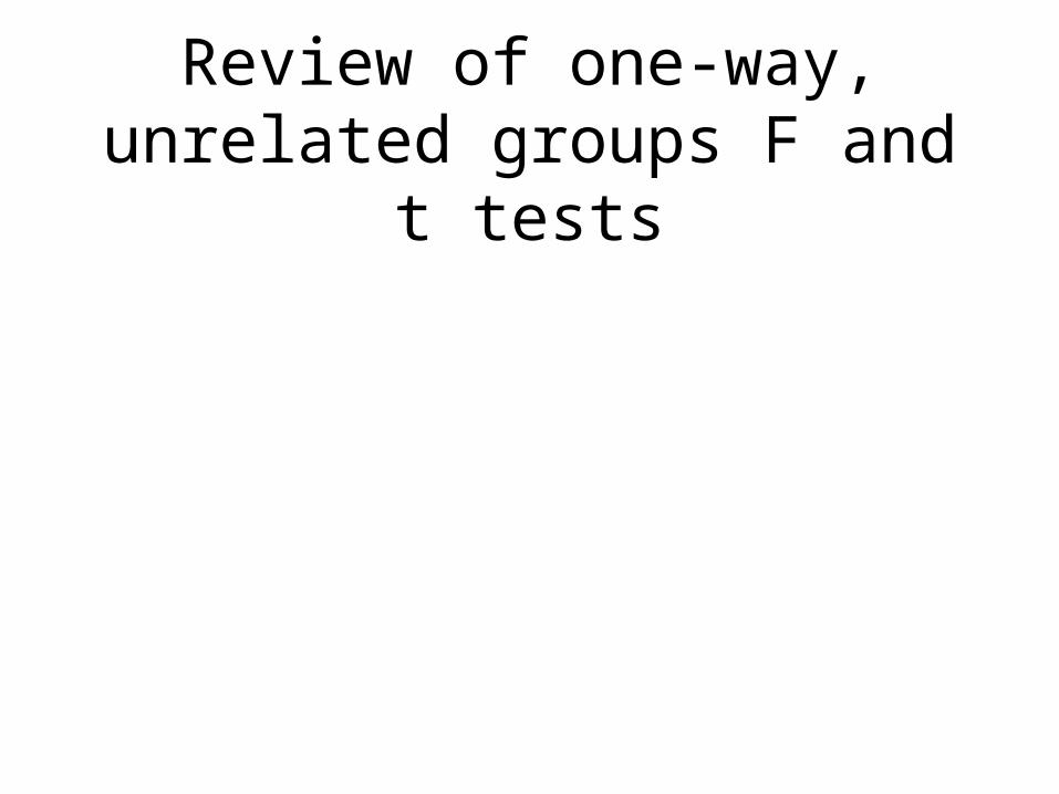
Simple Experiments

• Simple experiments have only a single independent variable with multiple levels.

• In simple experiments, participants are chosen independently. So participants in one group are unrelated to those in other groups.

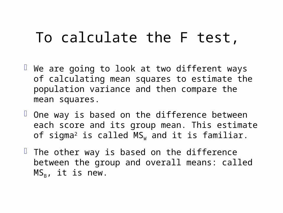
To calculate the F test,

We are going to look at two different ways of calculating mean squares to estimate the population variance and then compare the mean squares.

One way is based on the difference between each score and its group mean. This estimate of sigma2 is called MSW and it is familiar.

The other way is based on the difference between the group and overall means: called MSB, it is new.

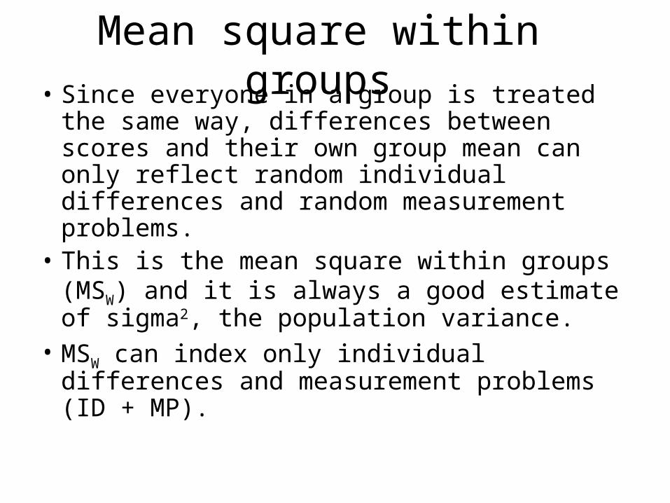
Mean square within groups• Since everyone in a group is treated the same

way, differences between scores and their own group mean can only reflect random individual differences and random measurement problems.

• This is the mean square within groups (MSW) and it is always a good estimate of sigma2, the population variance.

• MSW can index only individual differences and measurement problems (ID + MP).

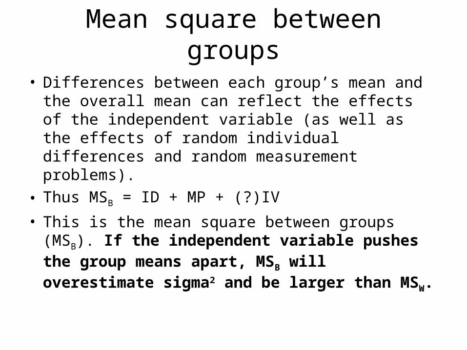
Mean square between groups

• Differences between each group’s mean and the overall mean can reflect the effects of the independent variable (as well as the effects of random individual differences and random measurement problems).

• Thus MSB = ID + MP + (?)IV

• This is the mean square between groups (MSB). If the independent variable pushes the group means apart, MSB will overestimate sigma2 and be larger than MSW.

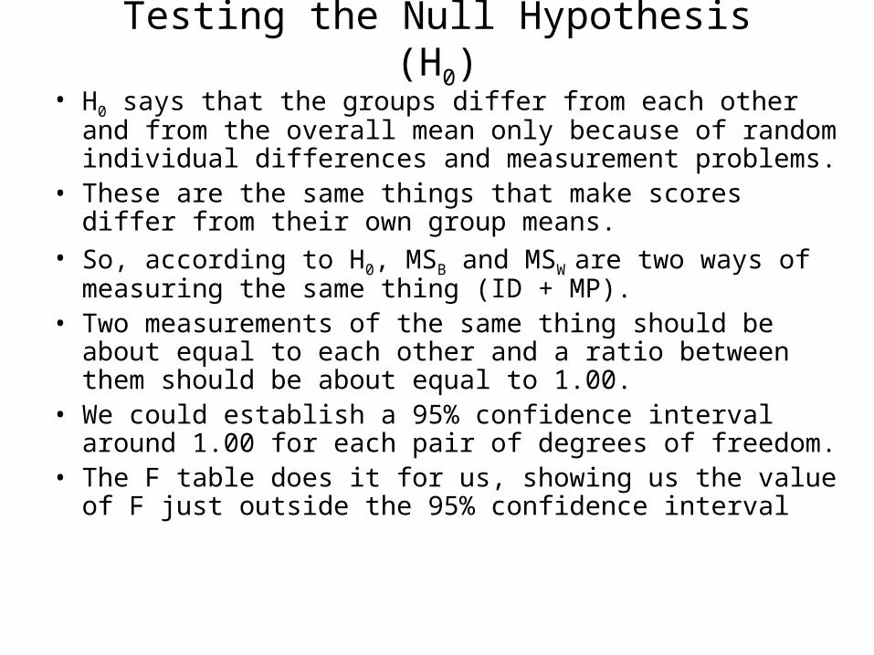
Testing the Null Hypothesis (H0)

• H0 says that the groups differ from each other and from the overall mean only because of random individual differences and measurement problems.

• These are the same things that make scores differ from their own group means.

• So, according to H0, MSB and MSW are two ways of measuring the same thing (ID + MP).

• Two measurements of the same thing should be about equal to each other and a ratio between them should be about equal to 1.00.

• We could establish a 95% confidence interval around 1.00 for each pair of degrees of freedom.

• The F table does it for us, showing us the value of F just outside the 95% confidence interval

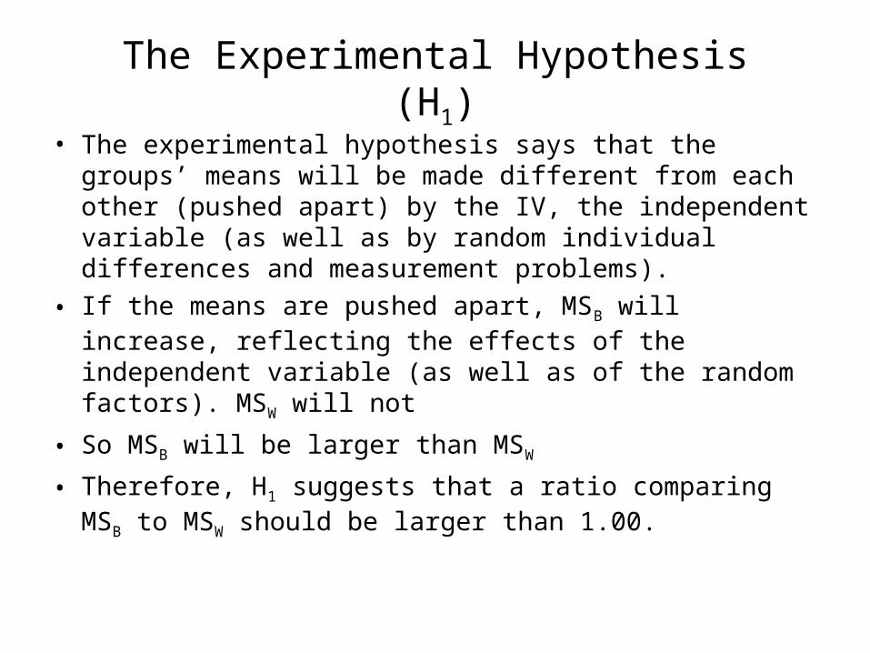
The Experimental Hypothesis (H1)

• The experimental hypothesis says that the groups’ means will be made different from each other (pushed apart) by the IV, the independent variable (as well as by random individual differences and measurement problems).

• If the means are pushed apart, MSB will increase, reflecting the effects of the independent variable (as well as of the random factors). MSW will not

• So MSB will be larger than MSW

• Therefore, H1 suggests that a ratio comparing MSB to MSW should be larger than 1.00.

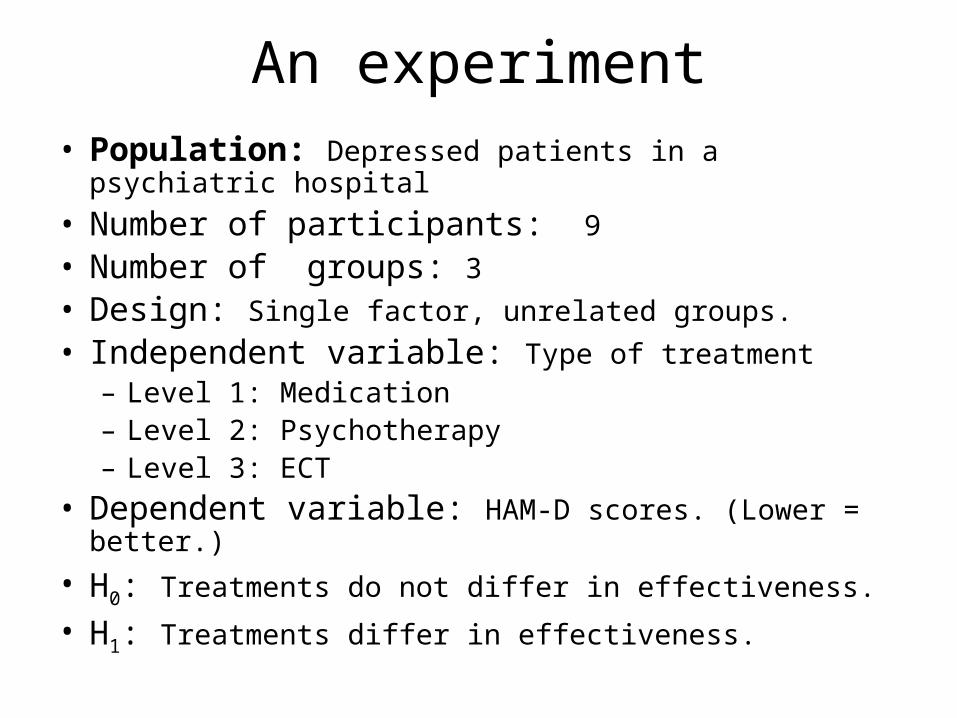
An experiment• Population: Depressed patients in a psychiatric hospital

• Number of participants: 9 • Number of groups: 3• Design: Single factor, unrelated groups.

• Independent variable: Type of treatment– Level 1: Medication– Level 2: Psychotherapy– Level 3: ECT

• Dependent variable: HAM-D scores. (Lower = better.)

• H0: Treatments do not differ in effectiveness.

• H1: Treatments differ in effectiveness.

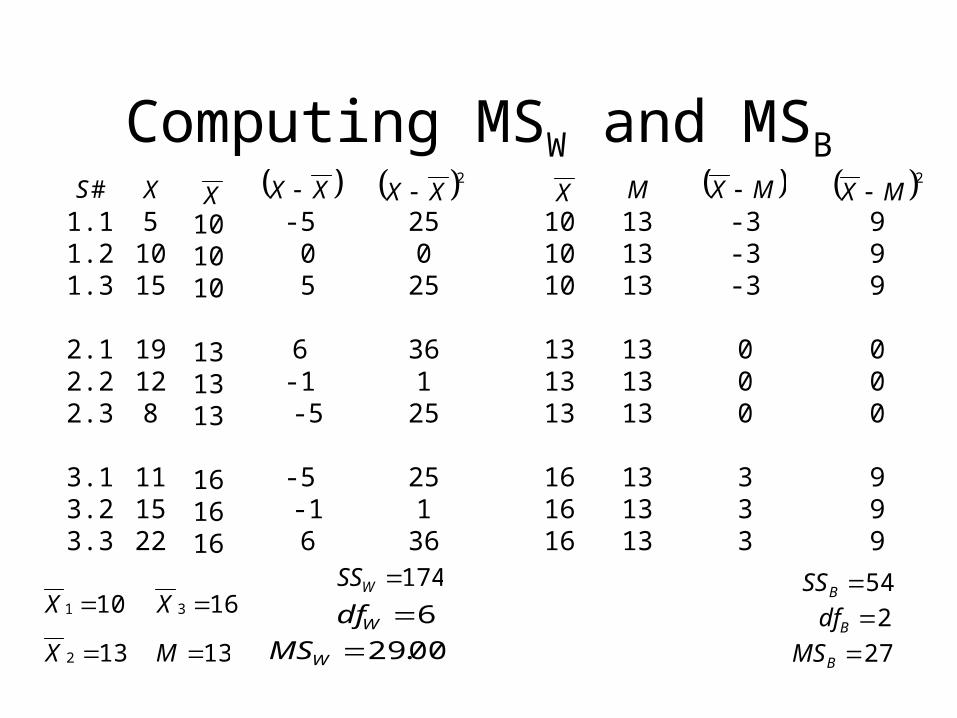
Computing MSW and MSB

1.11.21.3

2.12.22.3

3.13.23.3

51015

19128

111522

999

000

999

2MX -3-3-3

000

333

MX 101010

131313

161616

131313

131313

131313

MX250

25

361

25

251

36

2XX -5 0 5

6-1 -5

-5 -1 6

XX X#S

101010

131313

161616

X

101 X

132 X

163 X

13M

174WSS

6Wdf

00.29WMS

54BSS

2Bdf

27BMS

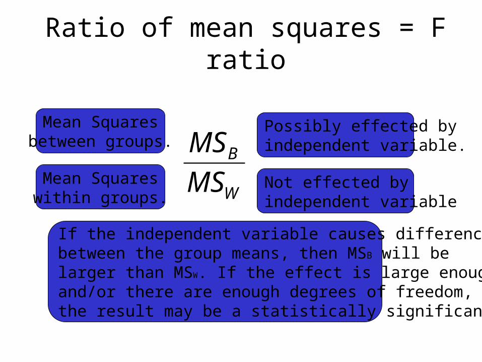
Ratio of mean squares = F ratio

W

B

MS

MSMean Squareswithin groups.

Mean Squaresbetween groups.

Possibly effected byindependent variable.

Not effected byindependent variable.

If the independent variable causes differencesbetween the group means, then MSB will belarger than MSW. If the effect is large enough and/or there are enough degrees of freedom, the result may be a statistically significant F ratio.

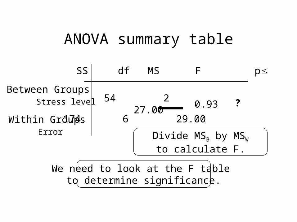
ANOVA summary table

Between GroupsStress level

Within GroupsError

54 2 27.00 174 6 29.00

0.93

SS df MS F p

?

We need to look at the F table to determine significance.

Divide MSB by MSW

to calculate F.

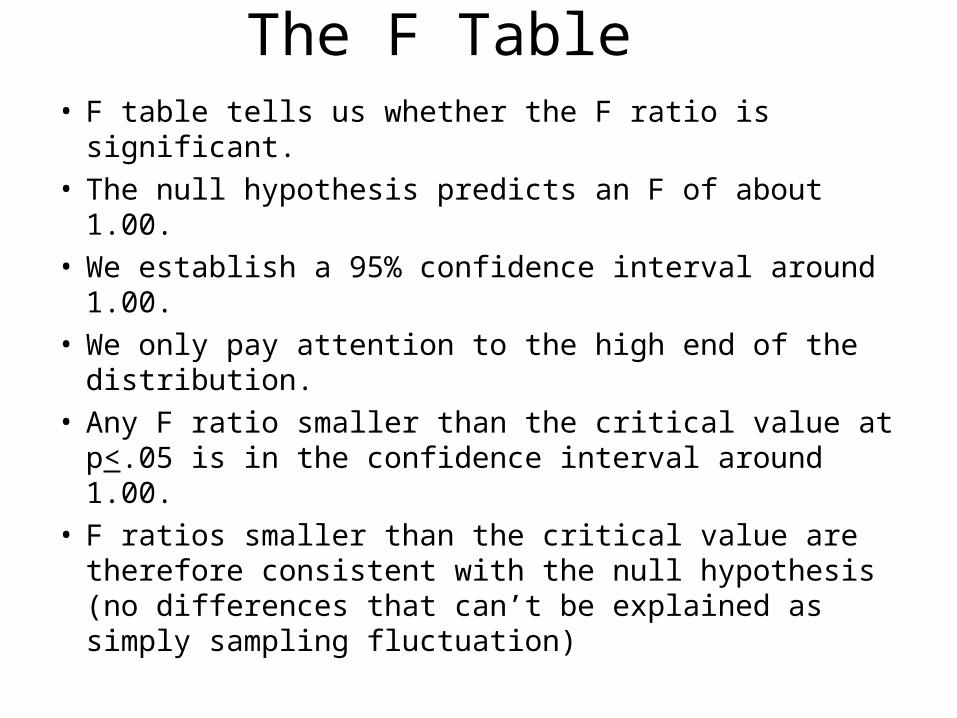
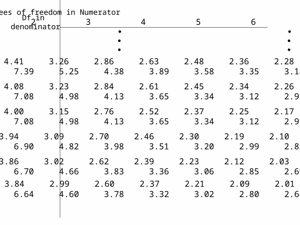
The F Table• F table tells us whether the F ratio is significant. • The null hypothesis predicts an F of about 1.00.• We establish a 95% confidence interval around 1.00. • We only pay attention to the high end of the

distribution.• Any F ratio smaller than the critical value at p<.05 is

in the confidence interval around 1.00.• F ratios smaller than the critical value are therefore

consistent with the null hypothesis (no differences that can’t be explained as simply sampling fluctuation)

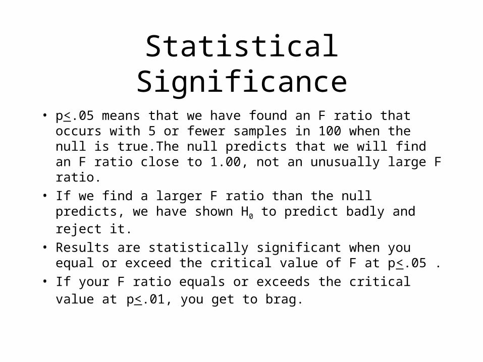
Statistical Significance

• p<.05 means that we have found an F ratio that occurs with 5 or fewer samples in 100 when the null is true.The null predicts that we will find an F ratio close to 1.00, not an unusually large F ratio.

• If we find a larger F ratio than the null predicts, we have shown H0 to predict badly and reject it.

• Results are statistically significant when you equal or exceed the critical value of F at p<.05 .

• If your F ratio equals or exceeds the critical value at p<.01, you get to brag.

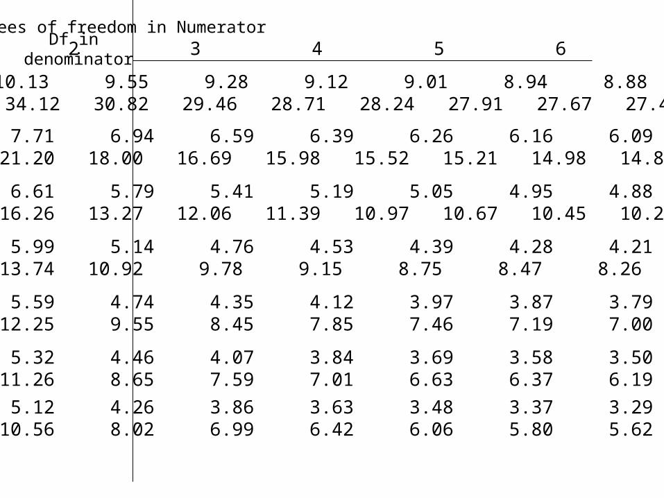
3 10.13 9.55 9.28 9.12 9.01 8.94 8.88 8.84 34.12 30.82 29.46 28.71 28.24 27.91 27.67 27.49

Degrees of freedom in Numerator 1 2 3 4 5 6 7 8 Df in

denominator

4 7.71 6.94 6.59 6.39 6.26 6.16 6.09 6.04 21.20 18.00 16.69 15.98 15.52 15.21 14.98 14.80

5 6.61 5.79 5.41 5.19 5.05 4.95 4.88 4.82 16.26 13.27 12.06 11.39 10.97 10.67 10.45 10.27

6 5.99 5.14 4.76 4.53 4.39 4.28 4.21 4.15 13.74 10.92 9.78 9.15 8.75 8.47 8.26 8.10

7 5.59 4.74 4.35 4.12 3.97 3.87 3.79 3.73 12.25 9.55 8.45 7.85 7.46 7.19 7.00 6.84

8 5.32 4.46 4.07 3.84 3.69 3.58 3.50 3.44 11.26 8.65 7.59 7.01 6.63 6.37 6.19 6.03

9 5.12 4.26 3.86 3.63 3.48 3.37 3.29 3.23 10.56 8.02 6.99 6.42 6.06 5.80 5.62 5.47

Degrees of freedom in Numerator 1 2 3 4 5 6 7 8 Df in

denominator

36 4.41 3.26 2.86 2.63 2.48 2.36 2.28 2.21 7.39 5.25 4.38 3.89 3.58 3.35 3.18 3.04

40 4.08 3.23 2.84 2.61 2.45 2.34 2.26 2.19 7.08 4.98 4.13 3.65 3.34 3.12 2.95 2.82

60 4.00 3.15 2.76 2.52 2.37 2.25 2.17 2.10 7.08 4.98 4.13 3.65 3.34 3.12 2.95 2.82

100 3.94 3.09 2.70 2.46 2.30 2.19 2.10 2.03 6.90 4.82 3.98 3.51 3.20 2.99 2.82 2.69

400 3.86 3.02 2.62 2.39 2.23 2.12 2.03 1.96 6.70 4.66 3.83 3.36 3.06 2.85 2.69 2.55

3.84 2.99 2.60 2.37 2.21 2.09 2.01 1.94 6.64 4.60 3.78 3.32 3.02 2.80 2.64 2.51

3 10.13 9.55 9.28 9.12 9.01 8.94 8.88 8.84 34.12 30.82 29.46 28.71 28.24 27.91 27.67 27.49

Degrees of freedom in Numerator 1 2 3 4 5 6 7 8 Df in

denominator

4 7.71 6.94 6.59 6.39 6.26 6.16 6.09 6.04 21.20 18.00 16.69 15.98 15.52 15.21 14.98 14.80

5 6.61 5.79 5.41 5.19 5.05 4.95 4.88 4.82 16.26 13.27 12.06 11.39 10.97 10.67 10.45 10.27

6 5.99 5.14 4.76 4.53 4.39 4.28 4.21 4.15 13.74 10.92 9.78 9.15 8.75 8.47 8.26 8.10

7 5.59 4.74 4.35 4.12 3.97 3.87 3.79 3.73 12.25 9.55 8.45 7.85 7.46 7.19 7.00 6.84

8 5.32 4.46 4.07 3.84 3.69 3.58 3.50 3.44 11.26 8.65 7.59 7.01 6.63 6.37 6.19 6.03

9 5.12 4.26 3.86 3.63 3.48 3.37 3.29 3.23 10.56 8.02 6.99 6.42 6.06 5.80 5.62 5.47

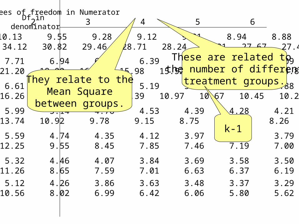
These are related to the number of different

treatment groups.They relate to theMean Square

between groups.

k-1

3 10.13 9.55 9.28 9.12 9.01 8.94 8.88 8.84 34.12 30.82 29.46 28.71 28.24 27.91 27.67 27.49

Degrees of freedom in Numerator 1 2 3 4 5 6 7 8 Df in

denominator

4 7.71 6.94 6.59 6.39 6.26 6.16 6.09 6.04 21.20 18.00 16.69 15.98 15.52 15.21 14.98 14.80

5 6.61 5.79 5.41 5.19 5.05 4.95 4.88 4.82 16.26 13.27 12.06 11.39 10.97 10.67 10.45 10.27

6 5.99 5.14 4.76 4.53 4.39 4.28 4.21 4.15 13.74 10.92 9.78 9.15 8.75 8.47 8.26 8.10

7 5.59 4.74 4.35 4.12 3.97 3.87 3.79 3.73 12.25 9.55 8.45 7.85 7.46 7.19 7.00 6.84

8 5.32 4.46 4.07 3.84 3.69 3.58 3.50 3.44 11.26 8.65 7.59 7.01 6.63 6.37 6.19 6.03

9 5.12 4.26 3.86 3.63 3.48 3.37 3.29 3.23 10.56 8.02 6.99 6.42 6.06 5.80 5.62 5.47

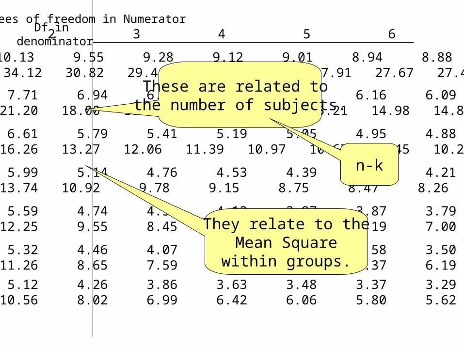
These are related to the number of subjects.

They relate to theMean Squarewithin groups.

n-k

3 10.13 9.55 9.28 9.12 9.01 8.94 8.88 8.84 34.12 30.82 29.46 28.71 28.24 27.91 27.67 27.49

Degrees of freedom in Numerator 1 2 3 4 5 6 7 8 Df in

denominator

4 7.71 6.94 6.59 6.39 6.26 6.16 6.09 6.04 21.20 18.00 16.69 15.98 15.52 15.21 14.98 14.80

5 6.61 5.79 5.41 5.19 5.05 4.95 4.88 4.82 16.26 13.27 12.06 11.39 10.97 10.67 10.45 10.27

6 5.99 5.14 4.76 4.53 4.39 4.28 4.21 4.15 13.74 10.92 9.78 9.15 8.75 8.47 8.26 8.10

7 5.59 4.74 4.35 4.12 3.97 3.87 3.79 3.73 12.25 9.55 8.45 7.85 7.46 7.19 7.00 6.84

8 5.32 4.46 4.07 3.84 3.69 3.58 3.50 3.44 11.26 8.65 7.59 7.01 6.63 6.37 6.19 6.03

9 5.12 4.26 3.86 3.63 3.48 3.37 3.29 3.23 10.56 8.02 6.99 6.42 6.06 5.80 5.62 5.47

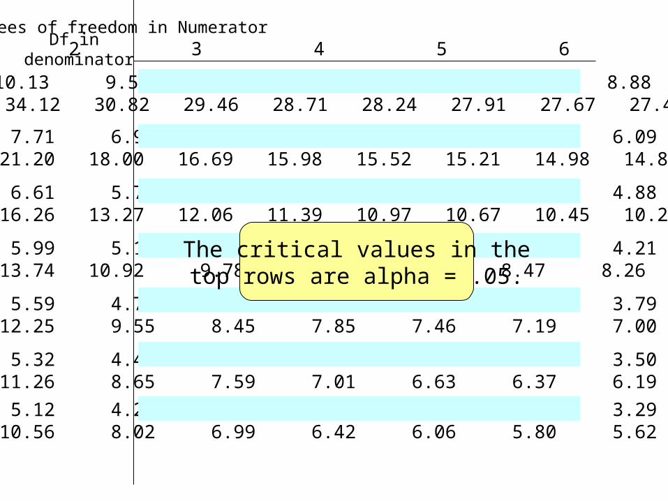
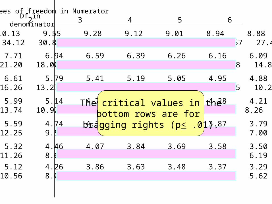
The critical values in thetop rows are alpha = .05.

3 10.13 9.55 9.28 9.12 9.01 8.94 8.88 8.84 34.12 30.82 29.46 28.71 28.24 27.91 27.67 27.49

Degrees of freedom in Numerator 1 2 3 4 5 6 7 8 Df in

denominator

4 7.71 6.94 6.59 6.39 6.26 6.16 6.09 6.04 21.20 18.00 16.69 15.98 15.52 15.21 14.98 14.80

5 6.61 5.79 5.41 5.19 5.05 4.95 4.88 4.82 16.26 13.27 12.06 11.39 10.97 10.67 10.45 10.27

6 5.99 5.14 4.76 4.53 4.39 4.28 4.21 4.15 13.74 10.92 9.78 9.15 8.75 8.47 8.26 8.10

7 5.59 4.74 4.35 4.12 3.97 3.87 3.79 3.73 12.25 9.55 8.45 7.85 7.46 7.19 7.00 6.84

8 5.32 4.46 4.07 3.84 3.69 3.58 3.50 3.44 11.26 8.65 7.59 7.01 6.63 6.37 6.19 6.03

9 5.12 4.26 3.86 3.63 3.48 3.37 3.29 3.23 10.56 8.02 6.99 6.42 6.06 5.80 5.62 5.47

The critical values in thebottom rows are for

bragging rights (p< .01).

3 10.13 9.55 9.28 9.12 9.01 8.94 8.88 8.84 34.12 30.82 29.46 28.71 28.24 27.91 27.67 27.49

Degrees of freedom in Numerator 1 2 3 4 5 6 7 8 Df in

denominator

4 7.71 6.94 6.59 6.39 6.26 6.16 6.09 6.04 21.20 18.00 16.69 15.98 15.52 15.21 14.98 14.80

5 6.61 5.79 5.41 5.19 5.05 4.95 4.88 4.82 16.26 13.27 12.06 11.39 10.97 10.67 10.45 10.27

6 5.99 5.14 4.76 4.53 4.39 4.28 4.21 4.15 13.74 10.92 9.78 9.15 8.75 8.47 8.26 8.10

7 5.59 4.74 4.35 4.12 3.97 3.87 3.79 3.73 12.25 9.55 8.45 7.85 7.46 7.19 7.00 6.84

8 5.32 4.46 4.07 3.84 3.69 3.58 3.50 3.44 11.26 8.65 7.59 7.01 6.63 6.37 6.19 6.03

9 5.12 4.26 3.86 3.63 3.48 3.37 3.29 3.23 10.56 8.02 6.99 6.42 6.06 5.80 5.62 5.47

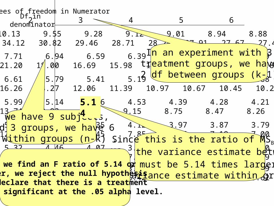
In an experiment with 3 treatment groups, we have 2 df between groups (k-1).

If we have 9 subjects, and 3 groups, we have 6df within groups (n-k) . Since this is the ratio of MSB to

MSW, the variance estimate between groups must be 5.14 times larger than the variance estimate within groups.

5.14

If we find an F ratio of 5.14 or larger, we reject the null hypothesis and declare that there is a treatment

effect, significant at the .05 alpha level.

ANOVA summary table

Between GroupsStress level

Within GroupsError

54 2 27.00 174 6 29.00

0.93

SS df MS F p

?

We need to look at the F table to determine significance.

Divide MSB by MSW

to calculate F.

3 10.13 9.55 9.28 9.12 9.01 8.94 8.88 8.84 34.12 30.82 29.46 28.71 28.24 27.91 27.67 27.49

Degrees of freedom in Numerator 1 2 3 4 5 6 7 8 Df in

denominator

4 7.71 6.94 6.59 6.39 6.26 6.16 6.09 6.04 21.20 18.00 16.69 15.98 15.52 15.21 14.98 14.80

5 6.61 5.79 5.41 5.19 5.05 4.95 4.88 4.82 16.26 13.27 12.06 11.39 10.97 10.67 10.45 10.27

6 5.99 5.14 4.76 4.53 4.39 4.28 4.21 4.15 13.74 10.92 9.78 9.15 8.75 8.47 8.26 8.10

7 5.59 4.74 4.35 4.12 3.97 3.87 3.79 3.73 12.25 9.55 8.45 7.85 7.46 7.19 7.00 6.84

8 5.32 4.46 4.07 3.84 3.69 3.58 3.50 3.44 11.26 8.65 7.59 7.01 6.63 6.37 6.19 6.03

9 5.12 4.26 3.86 3.63 3.48 3.37 3.29 3.23 10.56 8.02 6.99 6.42 6.06 5.80 5.62 5.47

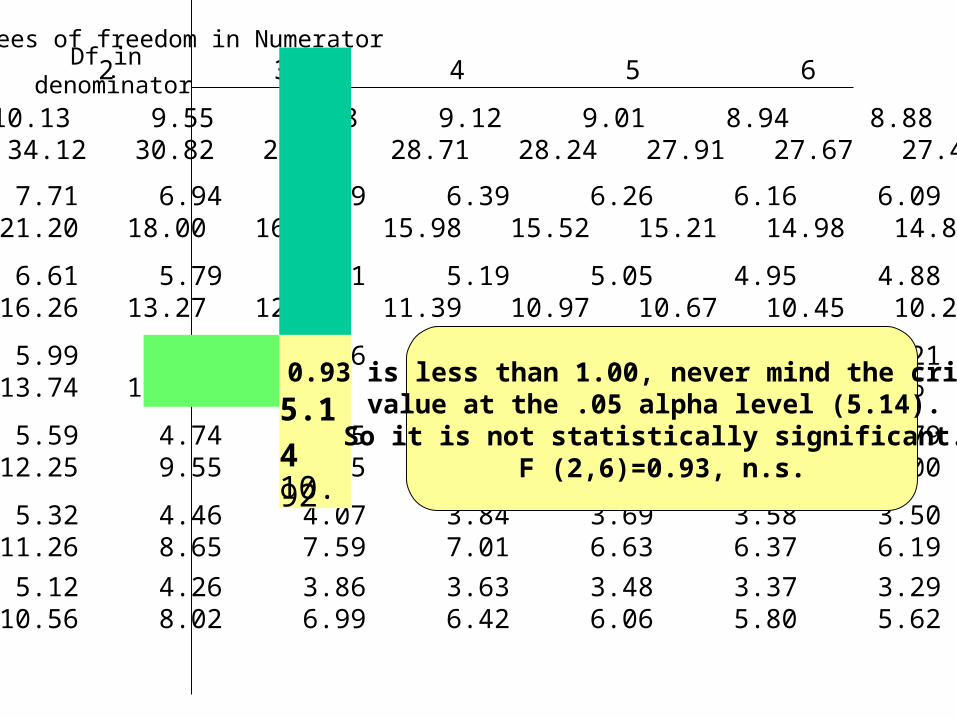
5.1410.92

0.93 is less than 1.00, never mind the criticalvalue at the .05 alpha level (5.14). So it is not statistically significant.

F (2,6)=0.93, n.s.

3 10.13 9.55 9.28 9.12 9.01 8.94 8.88 8.84 34.12 30.82 29.46 28.71 28.24 27.91 27.67 27.49

Degrees of freedom in Numerator 1 2 3 4 5 6 7 8 Df in

denominator

4 7.71 6.94 6.59 6.39 6.26 6.16 6.09 6.04 21.20 18.00 16.69 15.98 15.52 15.21 14.98 14.80

5 6.61 5.79 5.41 5.19 5.05 4.95 4.88 4.82 16.26 13.27 12.06 11.39 10.97 10.67 10.45 10.27

6 5.99 5.14 4.76 4.53 4.39 4.28 4.21 4.15 13.74 10.92 9.78 9.15 8.75 8.47 8.26 8.10

7 5.59 4.74 4.35 4.12 3.97 3.87 3.79 3.73 12.25 9.55 8.45 7.85 7.46 7.19 7.00 6.84

8 5.32 4.46 4.07 3.84 3.69 3.58 3.50 3.44 11.26 8.65 7.59 7.01 6.63 6.37 6.19 6.03

9 5.12 4.26 3.86 3.63 3.48 3.37 3.29 3.23 10.56 8.02 6.99 6.42 6.06 5.80 5.62 5.47

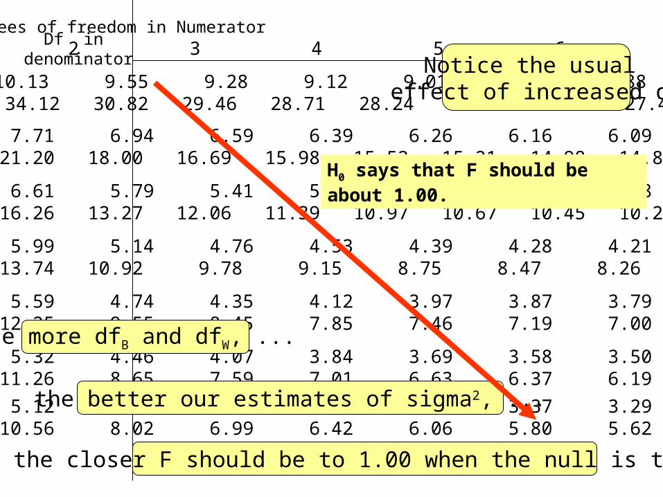
Notice the usual effect of increased df

The more dfB and dfW, ...

the better our estimates of sigma2, ...

the closer F should be to 1.00 when the null is true.

H0 says that F should be about 1.00.

The t test

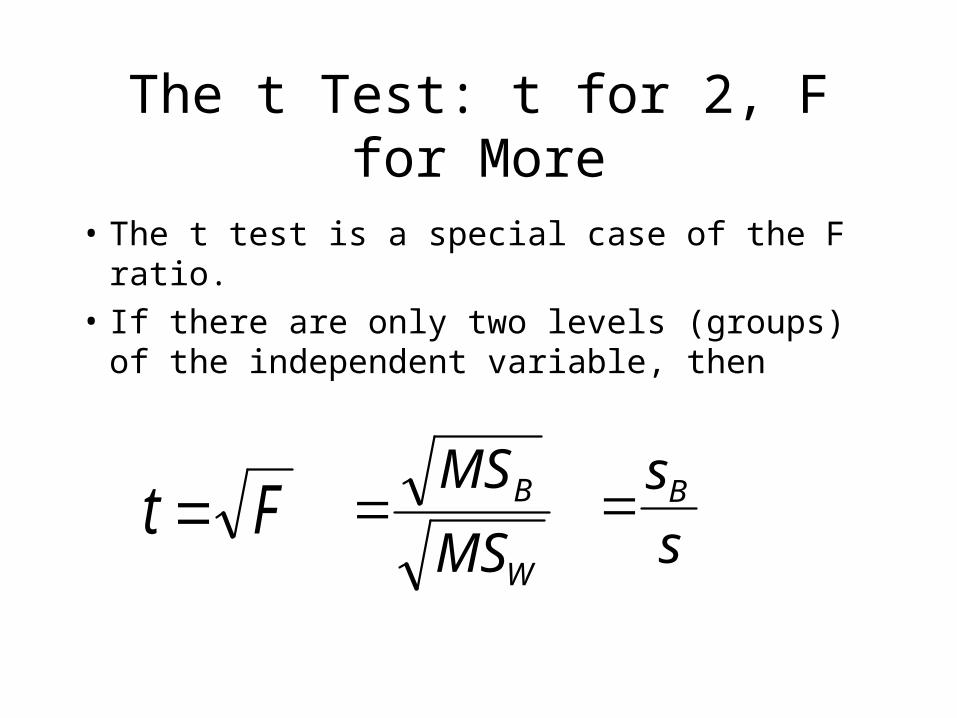
The t Test: t for 2, F for More

• The t test is a special case of the F ratio.

• If there are only two levels (groups) of the independent variable, then

Ft W

B

MS

MS

s

sB

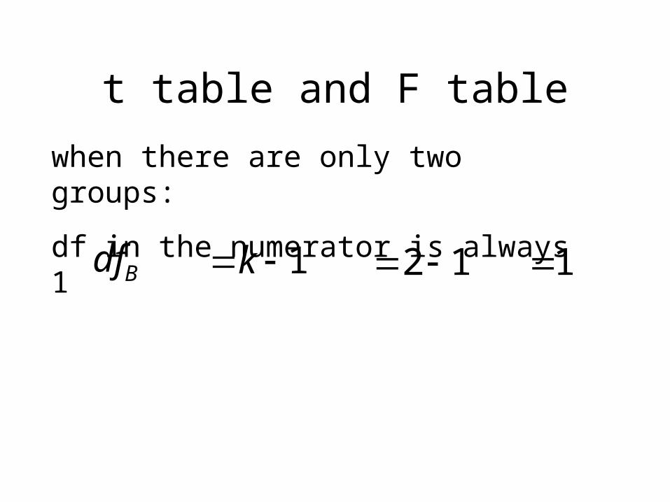
t table and F table

when there are only two groups:

df in the numerator is always 1

Bdf 1k 12 1

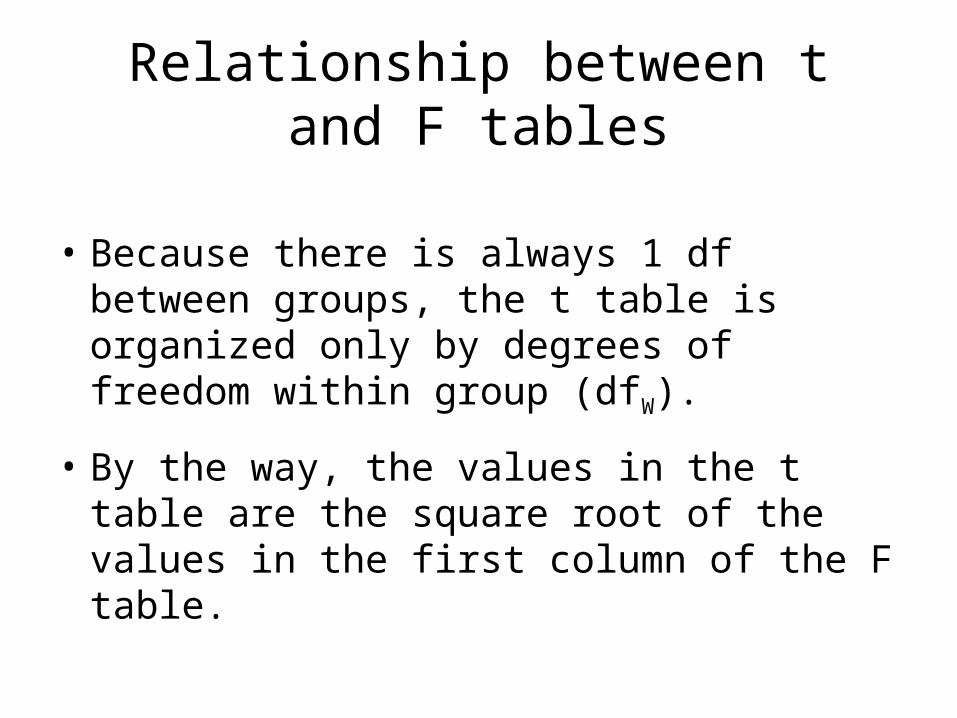
Relationship between t and F tables

• Because there is always 1 df between groups, the t table is organized only by degrees of freedom within group (dfW).

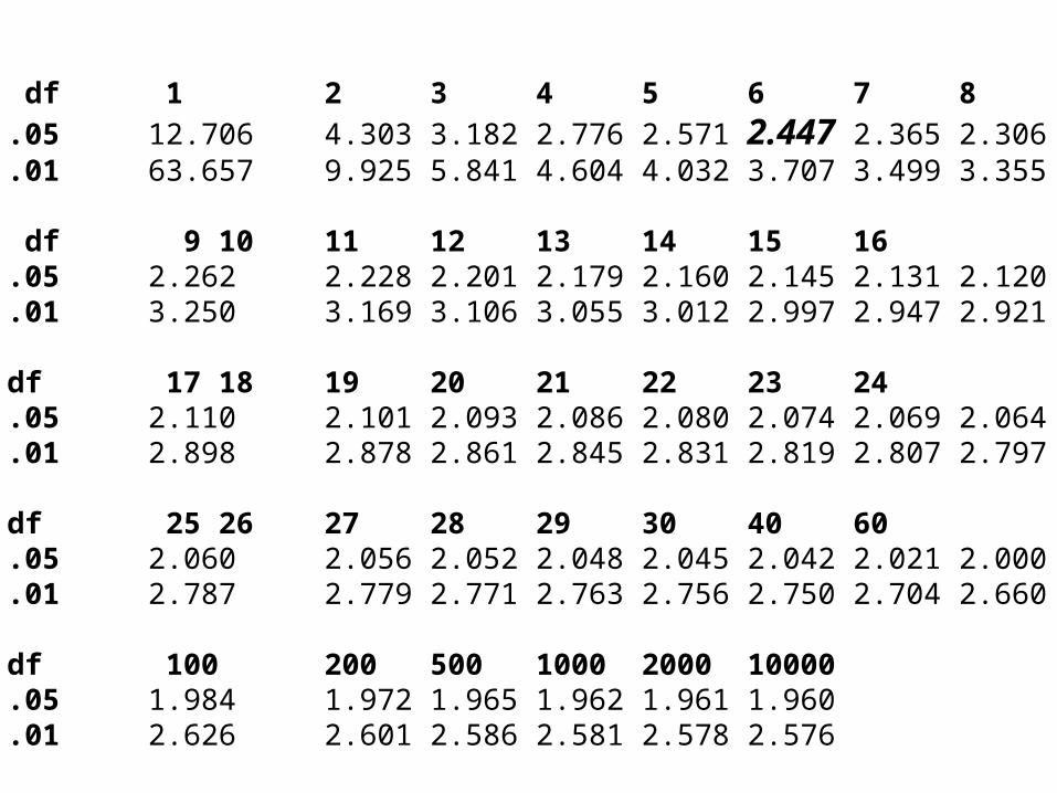
• By the way, the values in the t table are the square root of the values in the first column of the F table.

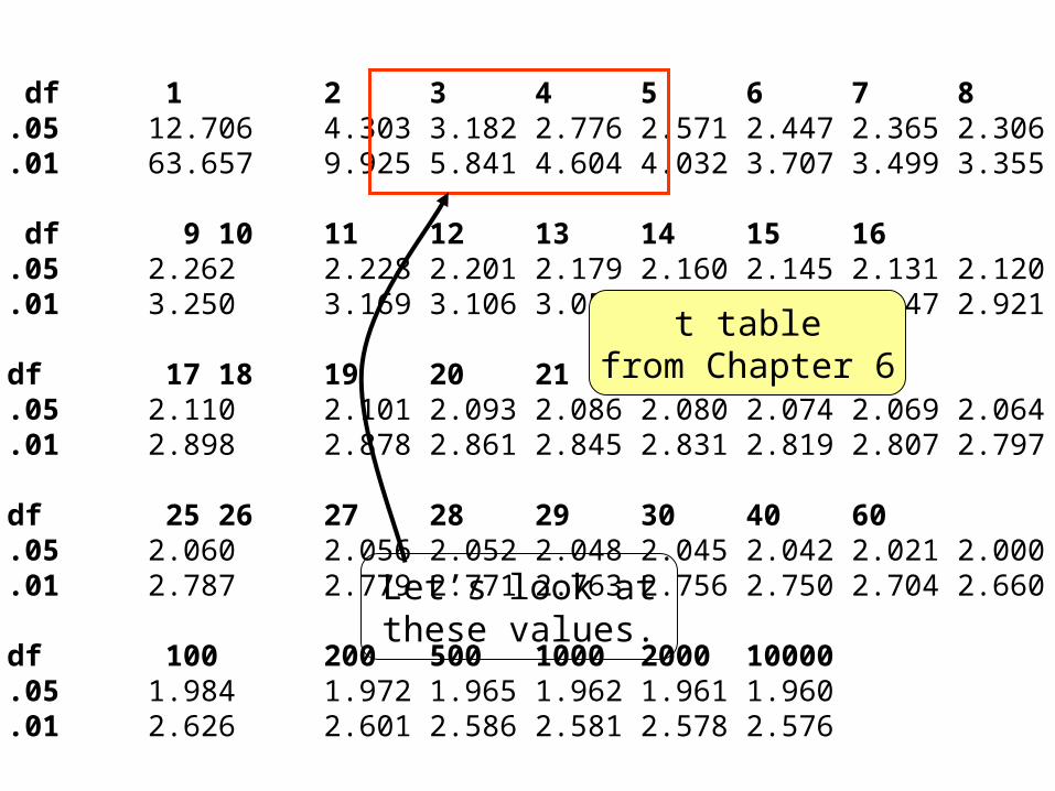
df 1 2 3 4 5 6 7 8.05 12.706 4.303 3.182 2.776 2.571 2.447 2.365 2.306.01 63.657 9.925 5.841 4.604 4.032 3.707 3.499 3.355

df 9 10 11 12 13 14 15 16.05 2.262 2.228 2.201 2.179 2.160 2.145 2.131 2.120.01 3.250 3.169 3.106 3.055 3.012 2.997 2.947 2.921

df 17 18 19 20 21 22 23 24.05 2.110 2.101 2.093 2.086 2.080 2.074 2.069 2.064.01 2.898 2.878 2.861 2.845 2.831 2.819 2.807 2.797

df 25 26 27 28 29 30 40 60.05 2.060 2.056 2.052 2.048 2.045 2.042 2.021 2.000.01 2.787 2.779 2.771 2.763 2.756 2.750 2.704 2.660

df 100 200 500 1000 2000 10000.05 1.984 1.972 1.965 1.962 1.961 1.960.01 2.626 2.601 2.586 2.581 2.578 2.576

t tablefrom Chapter 6

Let’s look atthese values.

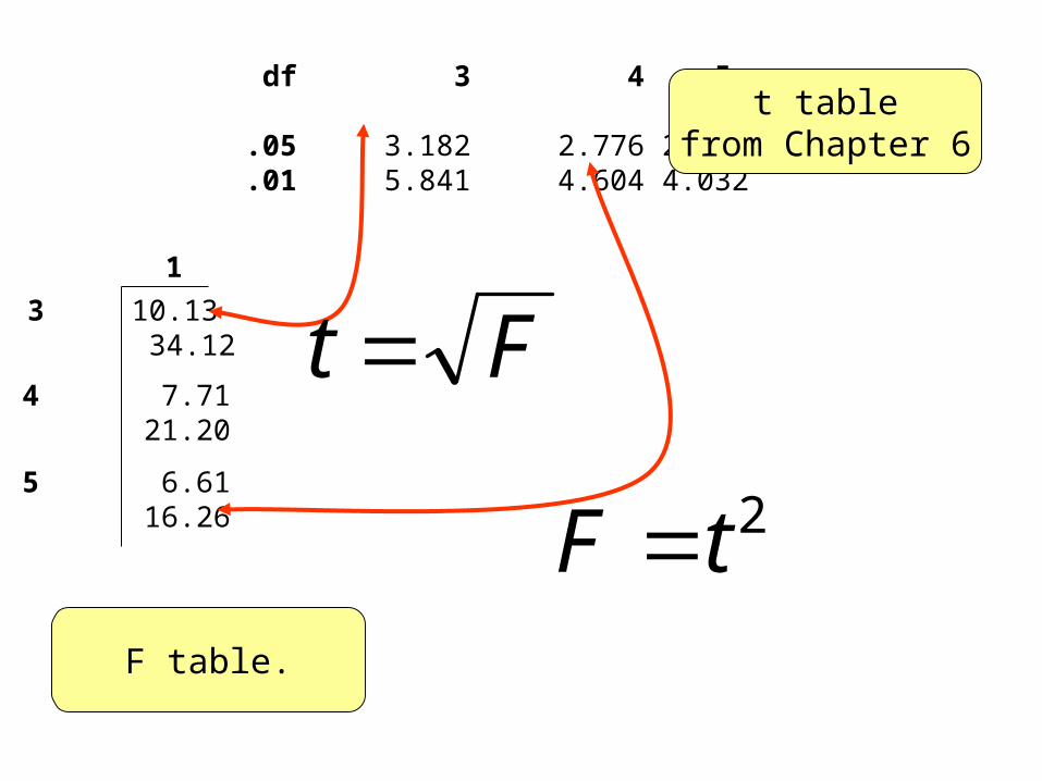
df 3 4 5.05 3.182 2.776 2.571.01 5.841 4.604 4.032

t tablefrom Chapter 6

F table.

3 10.13 34.12

4 7.71 21.20

5 6.61 16.26

1

Ft

2tF

You do this t test

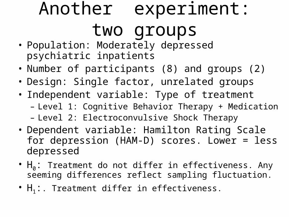
Another experiment: two groups• Population: Moderately depressed psychiatric

inpatients• Number of participants (8) and groups (2)• Design: Single factor, unrelated groups• Independent variable: Type of treatment

– Level 1: Cognitive Behavior Therapy + Medication– Level 2: Electroconvulsive Shock Therapy

• Dependent variable: Hamilton Rating Scale for depression (HAM-D) scores. Lower = less depressed

• H0: Treatment do not differ in effectiveness. Any seeming differences reflect sampling fluctuation.

• H1:. Treatment differ in effectiveness.

1.11.21.31.4

2.12.22.32.4

12141618

13161821

1111

1111

2MX -1-1-1-1

1 1 1 1

MX 15151515

21212121

16161616

16161616

MX9119

1611

16

2XX -3 -1 13

-4-1 1 4

XX X#S

00.8BSS

1Bdf

00.8BMS

00.54WSS

6Wdf

00.9WMS

Computing MSW and MSB

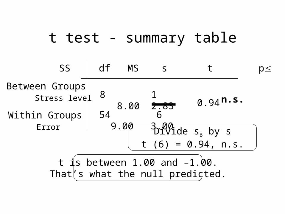
t test - summary table

Between GroupsStress level

Within GroupsError

8 1 8.00 2.83 54 6 9.00 3.00

0.94

SS df MS s t p

n.s.

t is between 1.00 and –1.00.That’s what the null predicted.

Divide sB by st (6) = 0.94, n.s.

Alternate Formats for F test problems.

How do you set up and solve this problem?

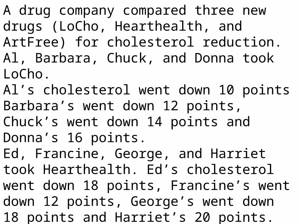
A drug company compared three new drugs (LoCho, Hearthealth, and ArtFree) for cholesterol reduction. Al, Barbara, Chuck, and Donna took LoCho. Al’s cholesterol went down 10 points Barbara’s went down 12 points, Chuck’s went down 14 points and Donna’s 16 points. Ed, Francine, George, and Harriet took Hearthealth. Ed’s cholesterol went down 18 points, Francine’s went down 12 points, George’s went down 18 points and Harriet’s 20 points. Ira, Jenny, Karl, and Linda took ArtFree. Ira’s cholesterol went down 28 points, Jenny’s went down 22 points, Karl’s went down 20 points and Linda’s 26 points.

This one is easy.

You just set up the within and between groups tables as usual.

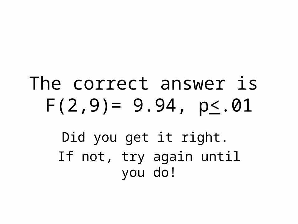
The correct answer is F(2,9)= 9.94, p<.01

Did you get it right.

If not, try again until you do!

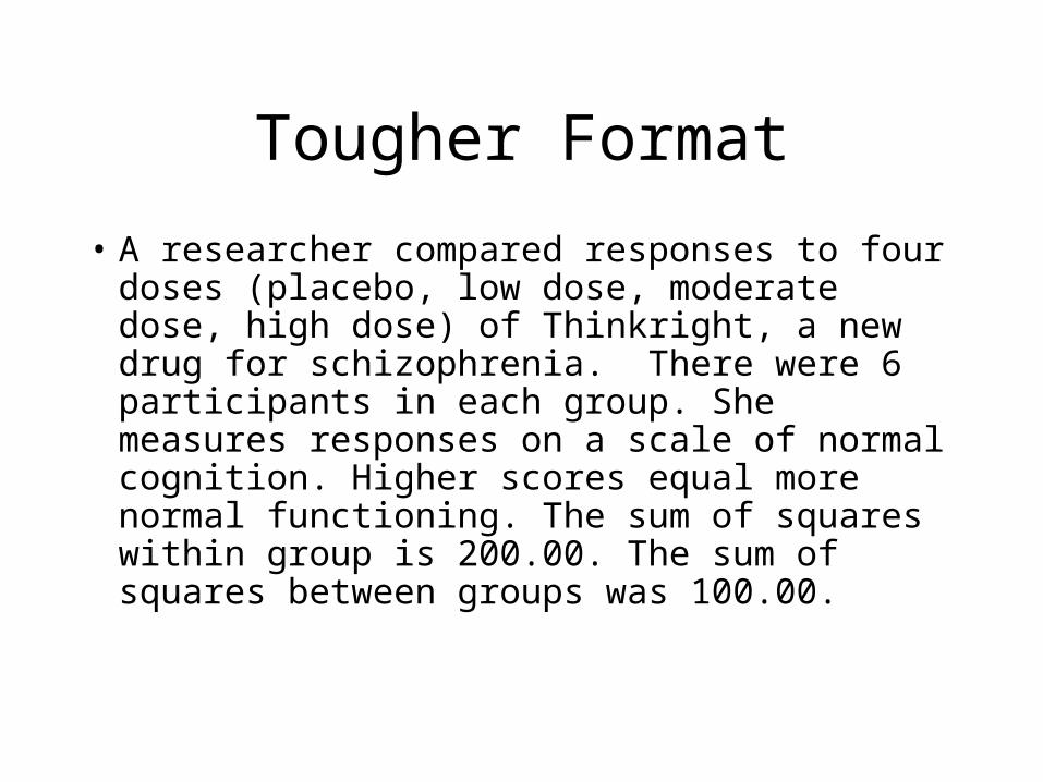
Tougher Format

• A researcher compared responses to four doses (placebo, low dose, moderate dose, high dose) of Thinkright, a new drug for schizophrenia. There were 6 participants in each group. She measures responses on a scale of normal cognition. Higher scores equal more normal functioning. The sum of squares within group is 200.00. The sum of squares between groups was 100.00.

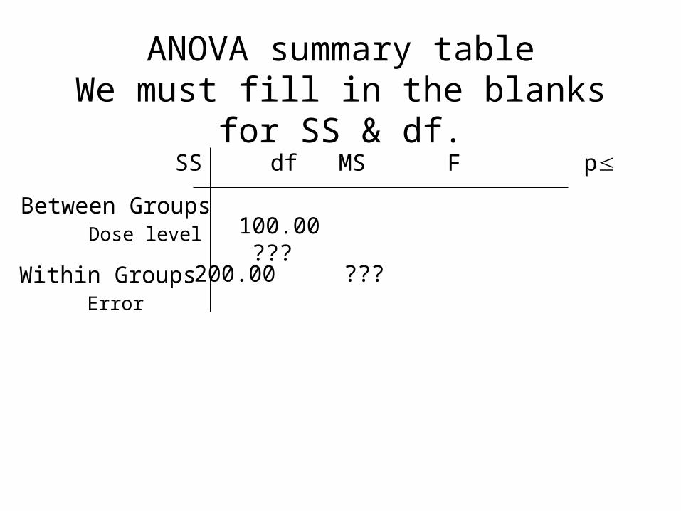
ANOVA summary tableWe must fill in the blanks for SS & df.

Between GroupsDose level

Within GroupsError

100.00 ???

200.00 ???

SS df MS F p

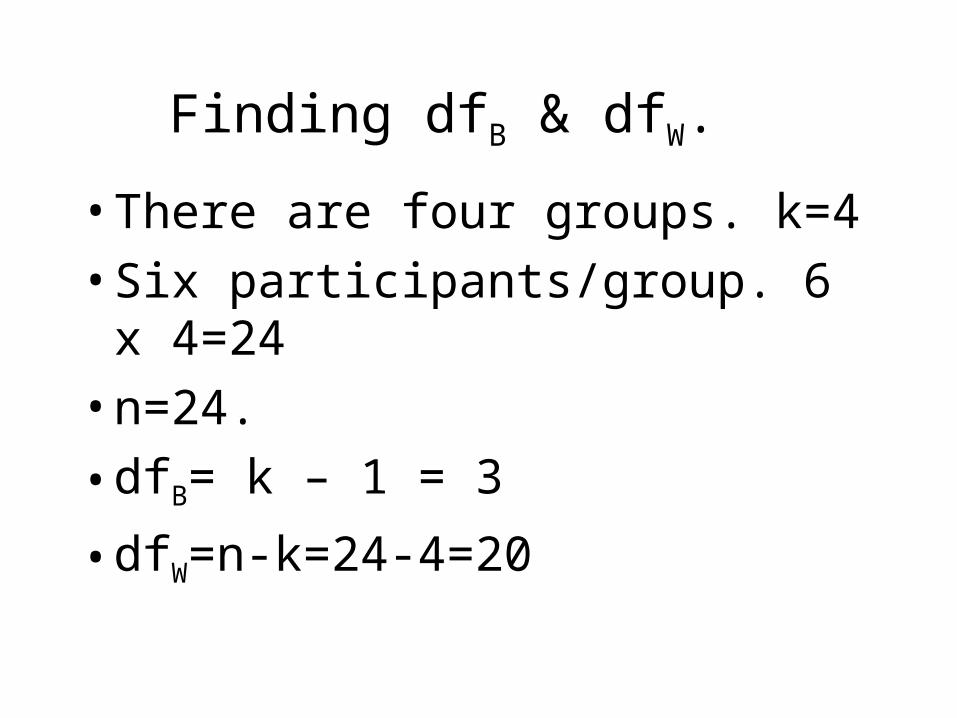
Finding dfB & dfW.

• There are four groups. k=4

• Six participants/group. 6 x 4=24

• n=24.

• dfB= k – 1 = 3

• dfW=n-k=24-4=20

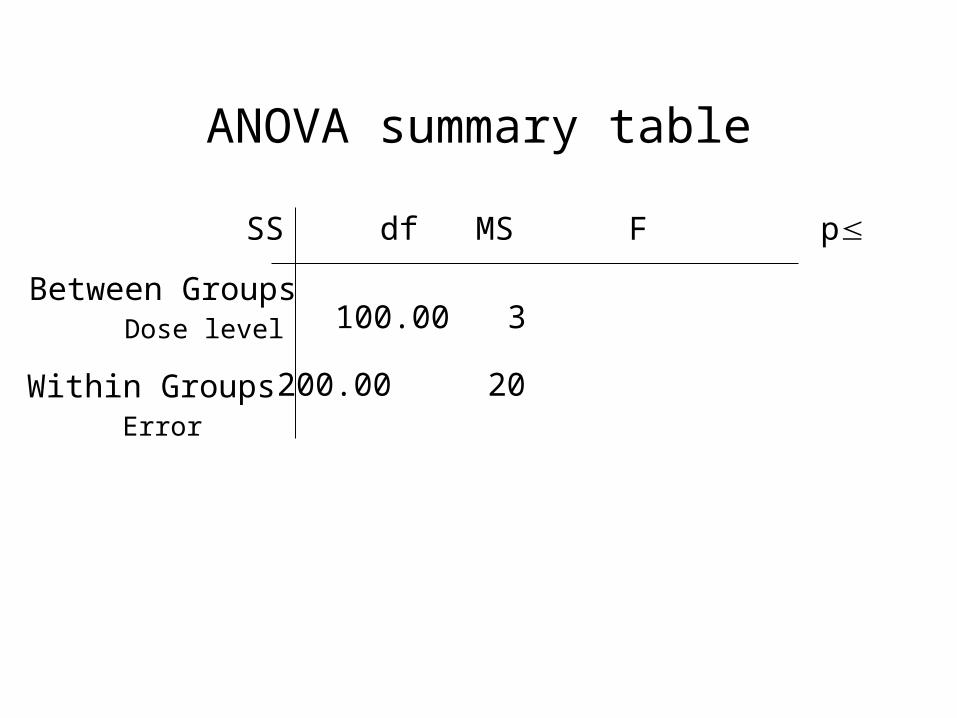
ANOVA summary table

Between GroupsDose level

Within GroupsError

100.00 3

200.00 20

SS df MS F p

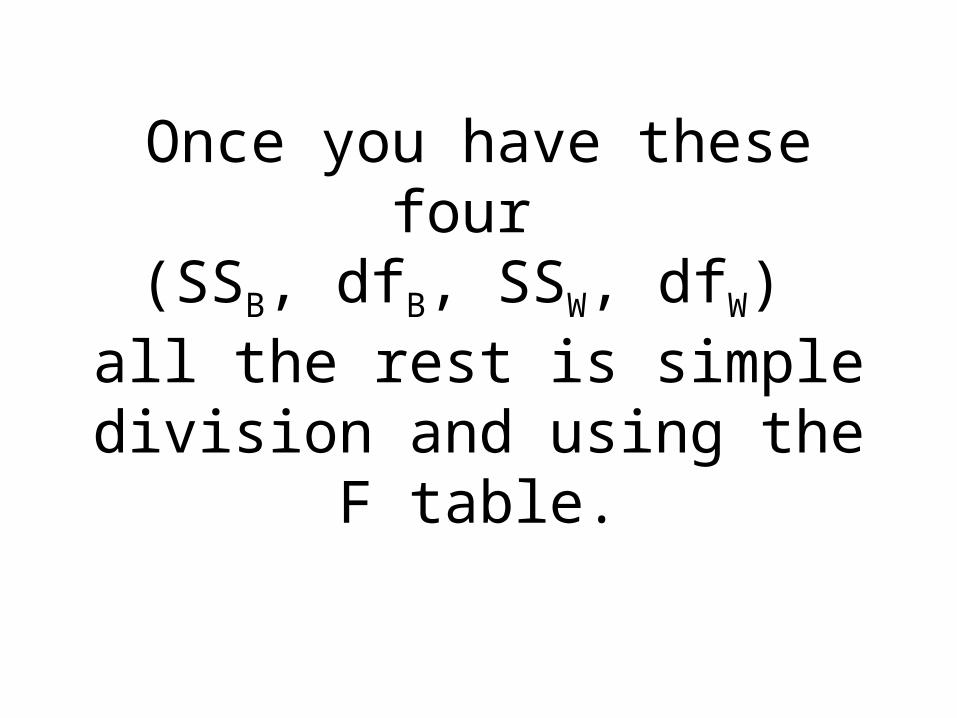
Once you have these four (SSB, dfB, SSW, dfW)

all the rest is simple division and using the F table.

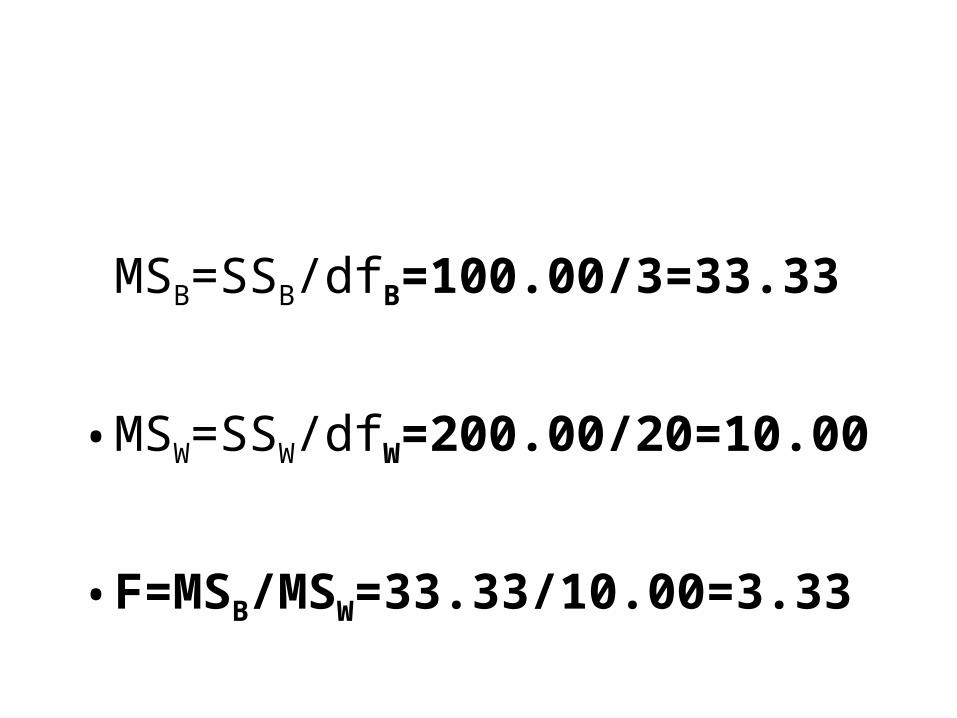
MSB=SSB/dfB=100.00/3=33.33

• MSW=SSW/dfW=200.00/20=10.00

• F=MSB/MSW=33.33/10.00=3.33

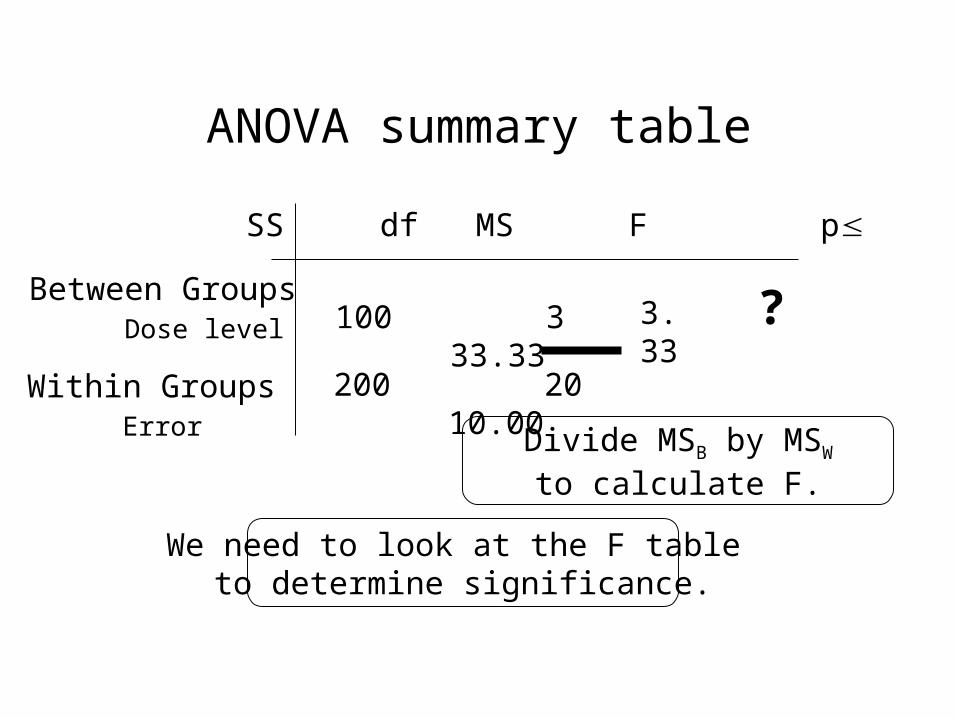
ANOVA summary table

Between GroupsDose level

Within GroupsError

100 3 33.33 200 20 10.00

3.33

SS df MS F p

?

We need to look at the F table to determine significance.

Divide MSB by MSW

to calculate F.

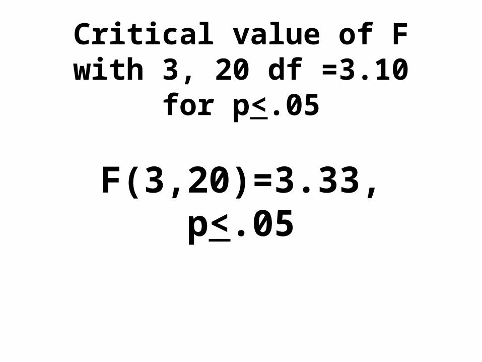
Critical value of F with 3, 20 df =3.10 for p<.05

F(3,20)=3.33, p<.05

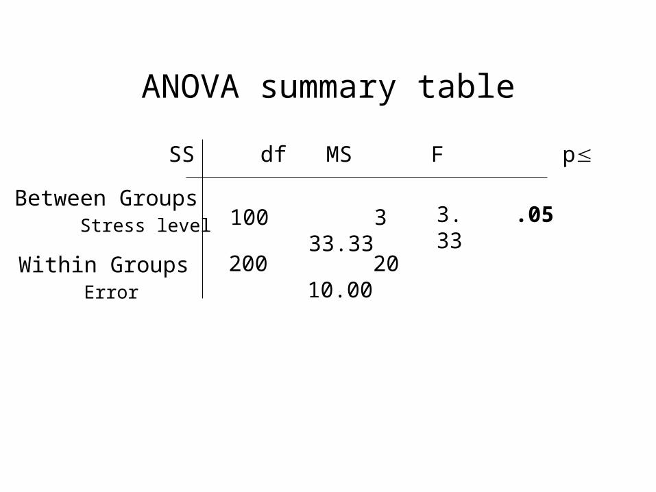
ANOVA summary table

Between GroupsStress level

Within GroupsError

100 3 33.33 200 20 10.00

3.33

SS df MS F p

.05

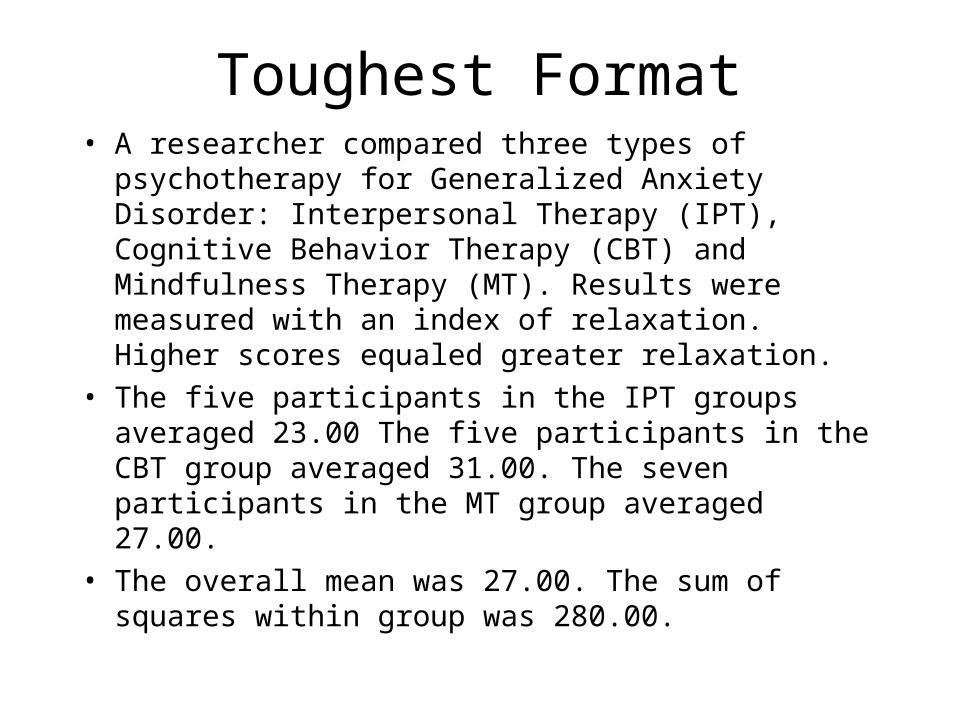
Toughest Format• A researcher compared three types of psychotherapy for

Generalized Anxiety Disorder: Interpersonal Therapy (IPT), Cognitive Behavior Therapy (CBT) and Mindfulness Therapy (MT). Results were measured with an index of relaxation. Higher scores equaled greater relaxation.

• The five participants in the IPT groups averaged 23.00 The five participants in the CBT group averaged 31.00. The seven participants in the MT group averaged 27.00.

• The overall mean was 27.00. The sum of squares within group was 280.00.

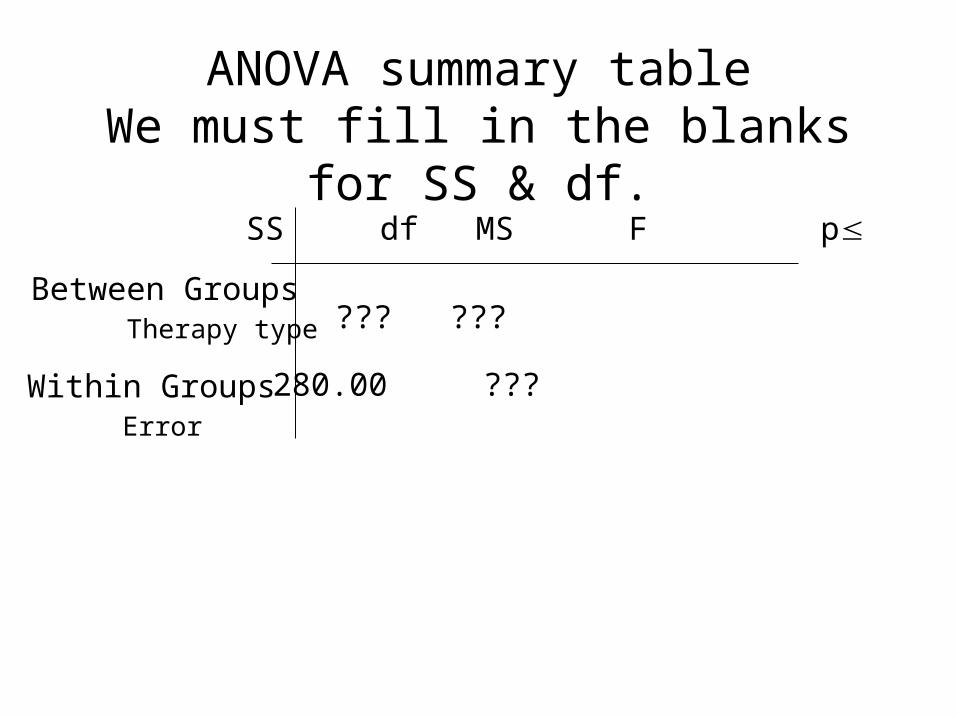
ANOVA summary tableWe must fill in the blanks for SS & df.

Between GroupsTherapy type

Within GroupsError

??? ???

280.00 ???

SS df MS F p

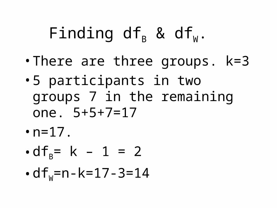
Finding dfB & dfW.

• There are three groups. k=3

• 5 participants in two groups 7 in the remaining one. 5+5+7=17

• n=17.

• dfB= k – 1 = 2

• dfW=n-k=17-3=14

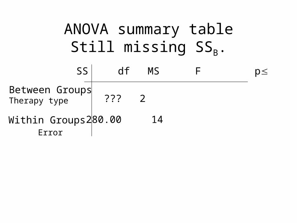
ANOVA summary tableStill missing SSB.

Between GroupsTherapy type

Within GroupsError

??? 2

280.00 14

SS df MS F p

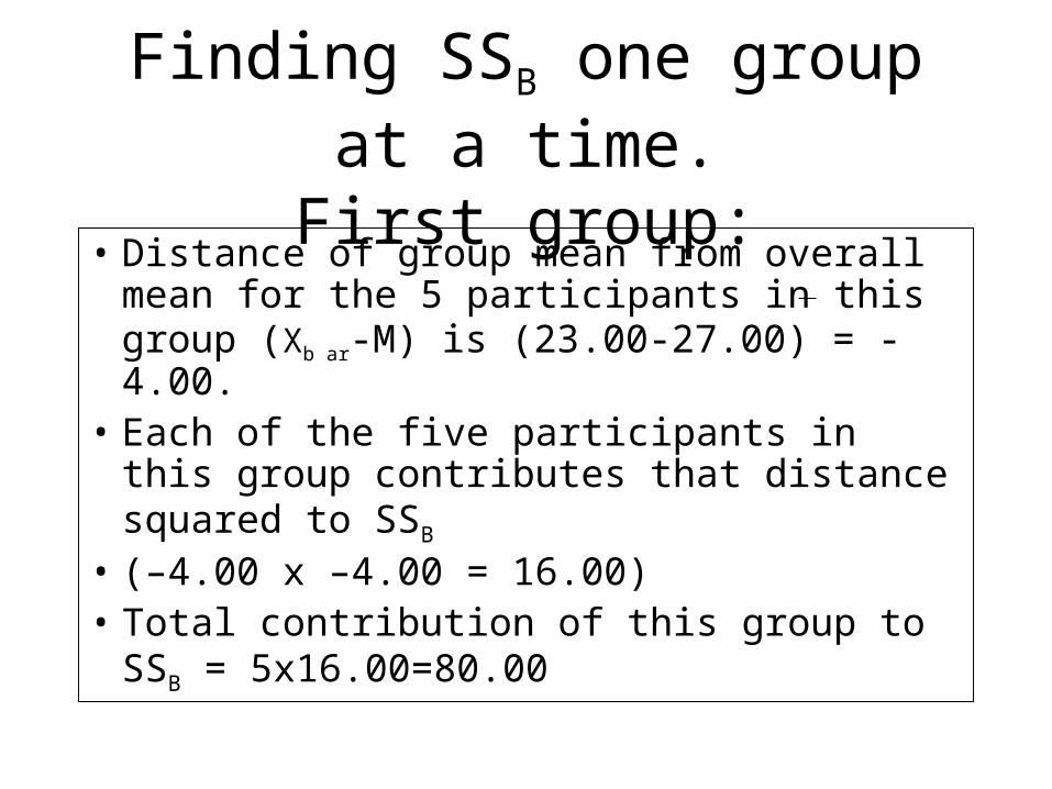
Finding SSB one group at a time.First group:

• Distance of group mean from overall mean for the 5 participants in this group (Xb ar-M) is (23.00-27.00) = -4.00.

• Each of the five participants in this group contributes that distance squared to SSB

• (–4.00 x –4.00 = 16.00)• Total contribution of this group to SSB =

5x16.00=80.00

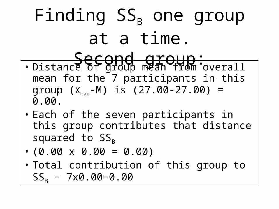
Finding SSB one group at a time.Second group:

• Distance of group mean from overall mean for the 7 participants in this group (Xbar-M) is (27.00-27.00) = 0.00.

• Each of the seven participants in this group contributes that distance squared to SSB

• (0.00 x 0.00 = 0.00)• Total contribution of this group to SSB =

7x0.00=0.00

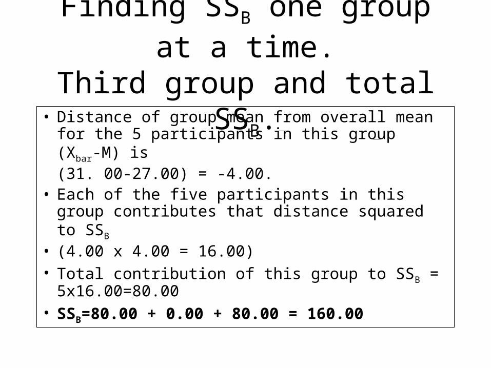
Finding SSB one group at a time.Third group and total SSB.

• Distance of group mean from overall mean for the 5 participants in this group (Xbar-M) is (31. 00-27.00) = -4.00.

• Each of the five participants in this group contributes that distance squared to SSB

• (4.00 x 4.00 = 16.00)• Total contribution of this group to SSB =

5x16.00=80.00• SSB=80.00 + 0.00 + 80.00 = 160.00

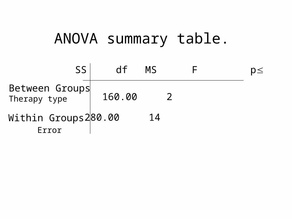
ANOVA summary table.

Between GroupsTherapy type

Within GroupsError

160.00 2

280.00 14

SS df MS F p

Once you have these four (SSB, dfB, SSW, dfW)

all the rest is simple division and using the F table.

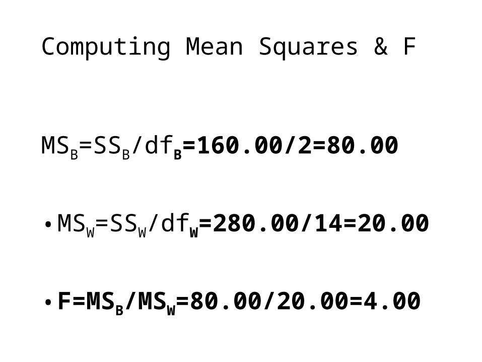
Computing Mean Squares & F

MSB=SSB/dfB=160.00/2=80.00

• MSW=SSW/dfW=280.00/14=20.00

• F=MSB/MSW=80.00/20.00=4.00

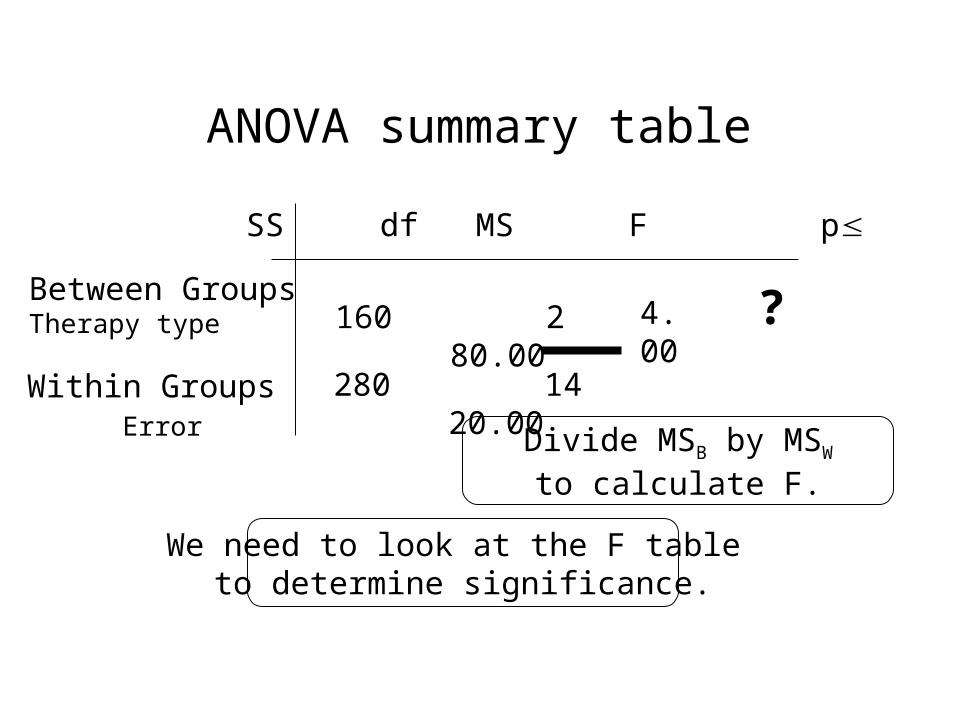
ANOVA summary table

Between GroupsTherapy type

Within GroupsError

160 2 80.00 280 14 20.00

4.00

SS df MS F p

?

We need to look at the F table to determine significance.

Divide MSB by MSW

to calculate F.

Critical value of F with 2,14 df =3.74 for p<.05

F(2,14)=4.00, p<.05

ANOVA summary table

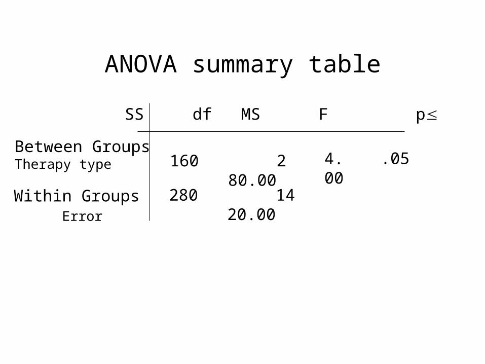
Between GroupsTherapy type

Within GroupsError

160 2 80.00 280 14 20.00

4.00

SS df MS F p

.05

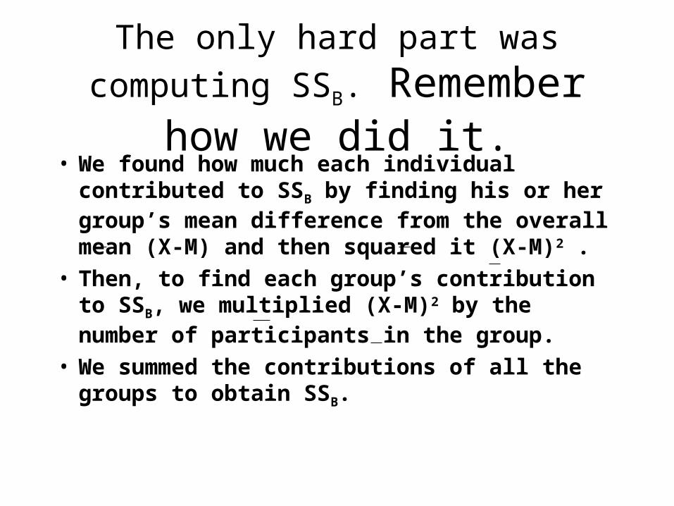
The only hard part was computing SSB. Remember how we did it.

• We found how much each individual contributed to SSB by finding his or her group’s mean difference from the overall mean (X-M) and then squared it (X-M)2 .

• Then, to find each group’s contribution to SSB, we multiplied (X-M)2 by the number of participants in the group.

• We summed the contributions of all the groups to obtain SSB.

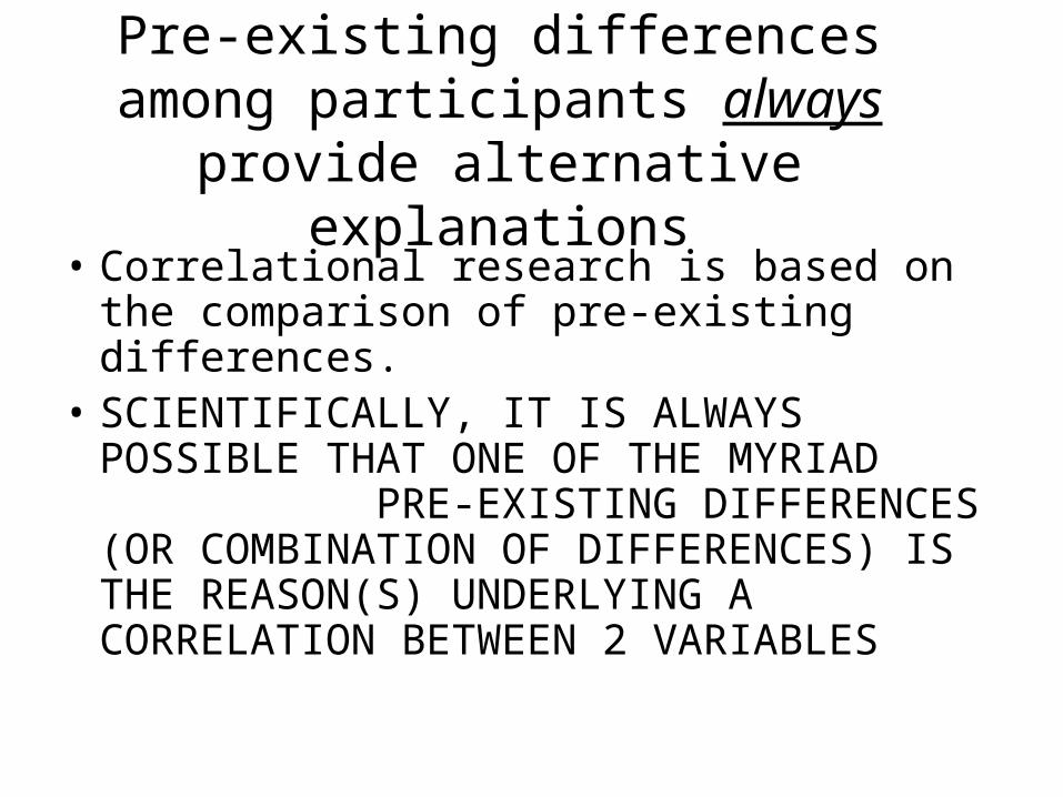
Pre-existing differences among participants always provide alternative

explanations• Correlational research is based on the

comparison of pre-existing differences.• SCIENTIFICALLY, IT IS ALWAYS

POSSIBLE THAT ONE OF THE MYRIAD PRE-EXISTING DIFFERENCES (OR COMBINATION OF DIFFERENCES) IS THE REASON(S) UNDERLYING A CORRELATION BETWEEN 2 VARIABLES

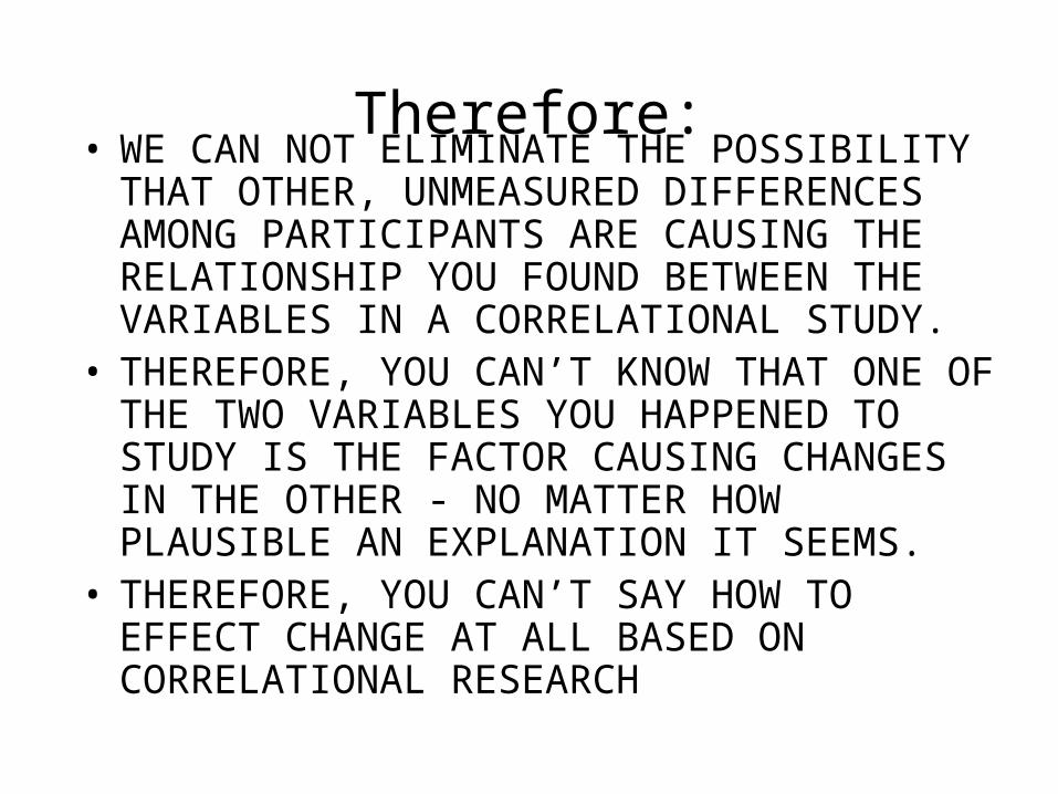
Therefore:• WE CAN NOT ELIMINATE THE POSSIBILITY

THAT OTHER, UNMEASURED DIFFERENCES AMONG PARTICIPANTS ARE CAUSING THE RELATIONSHIP YOU FOUND BETWEEN THE VARIABLES IN A CORRELATIONAL STUDY.

• THEREFORE, YOU CAN’T KNOW THAT ONE OF THE TWO VARIABLES YOU HAPPENED TO STUDY IS THE FACTOR CAUSING CHANGES IN THE OTHER - NO MATTER HOW PLAUSIBLE AN EXPLANATION IT SEEMS.

• THEREFORE, YOU CAN’T SAY HOW TO EFFECT CHANGE AT ALL BASED ON CORRELATIONAL RESEARCH

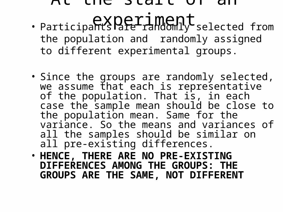
At the start of an experiment• Participants are randomly selected from the

population and randomly assigned to different experimental groups.

• Since the groups are randomly selected, we assume that each is representative of the population. That is, in each case the sample mean should be close to the population mean. Same for the variance. So the means and variances of all the samples should be similar on all pre-existing differences.

• HENCE, THERE ARE NO PRE-EXISTING DIFFERENCES AMONG THE GROUPS: THE GROUPS ARE THE SAME, NOT DIFFERENT

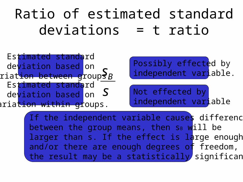
Ratio of estimated standard deviations = t ratio

s

sBEstimated standarddeviation based on

variation within groups.

Estimated standarddeviation based on

variation between groups.

Possibly effected byindependent variable.

Not effected byindependent variable.

If the independent variable causes differencesbetween the group means, then sB will belarger than s. If the effect is large enough and/or there are enough degrees of freedom, the result may be a statistically significant t test.

df 1 2 3 4 5 6 7 8

.05 12.706 4.303 3.182 2.776 2.571 2.447 2.365 2.306

.01 63.657 9.925 5.841 4.604 4.032 3.707 3.499 3.355

df 9 10 11 12 13 14 15 16.05 2.262 2.228 2.201 2.179 2.160 2.145 2.131 2.120.01 3.250 3.169 3.106 3.055 3.012 2.997 2.947 2.921

df 17 18 19 20 21 22 23 24.05 2.110 2.101 2.093 2.086 2.080 2.074 2.069 2.064.01 2.898 2.878 2.861 2.845 2.831 2.819 2.807 2.797

df 25 26 27 28 29 30 40 60.05 2.060 2.056 2.052 2.048 2.045 2.042 2.021 2.000.01 2.787 2.779 2.771 2.763 2.756 2.750 2.704 2.660

df 100 200 500 1000 2000 10000.05 1.984 1.972 1.965 1.962 1.961 1.960.01 2.626 2.601 2.586 2.581 2.578 2.576

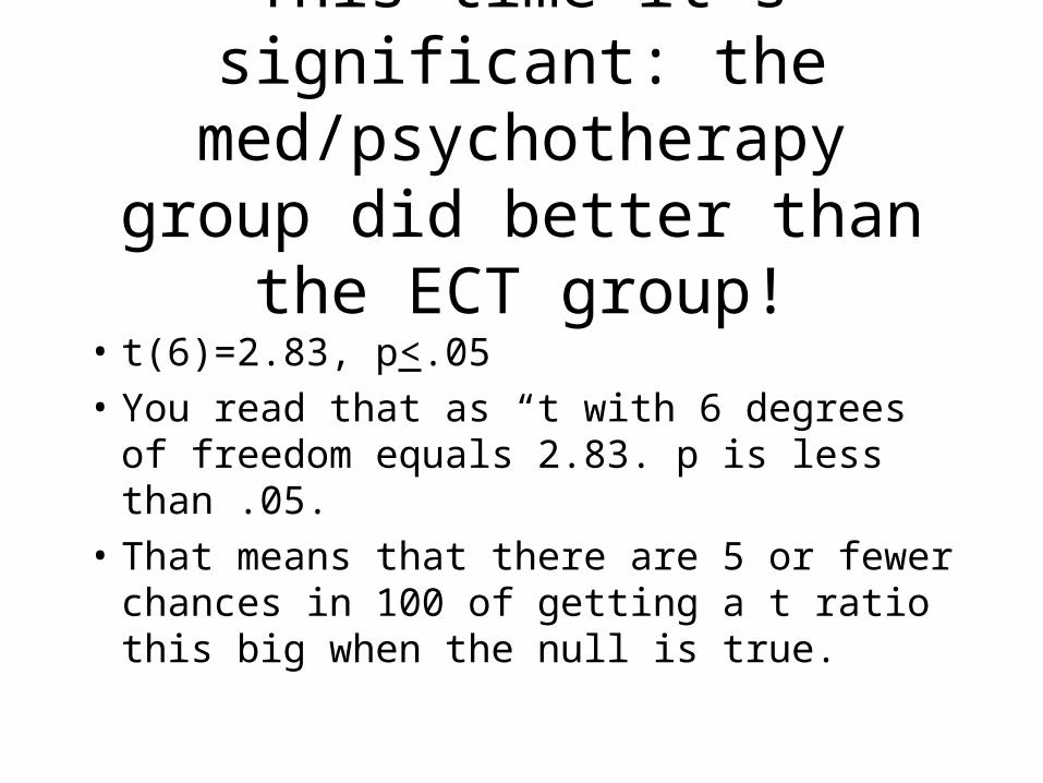
This time it’s significant: the med/psychotherapy group did

better than the ECT group!

• t(6)=2.83, p<.05

• You read that as “t with 6 degrees of freedom equals 2.83. p is less than .05.

• That means that there are 5 or fewer chances in 100 of getting a t ratio this big when the null is true.