Chapter 9 Integer Programming

Companion slides of Applied Mathematical Programming

by Bradley, Hax, and Magnanti (Addison-Wesley, 1977)

prepared by José Fernando Oliveira

Maria Antónia Carravilla

What are integer-programming problems?

• In many applications, integrality restrictions reflect natural indivisibilities of the problem under study. For example, when deciding how many nuclear aircraft carriers to have in the U.S. Navy, fractional solutions clearly are meaningless. In these situations, the decision variables are inherently integral by the nature of the decision-making problem.

What are integer-programming problems?

• Linear programming problems in which fractional solutions are not realistic. – Mixed integer programs when some, but not all,

variables are restricted to be integer. – Pure integer programs when all decision variables

must be integers. – Binary programs when all decision variables must

be either 0 or 1.

SOME INTEGER-PROGRAMMING MODELS

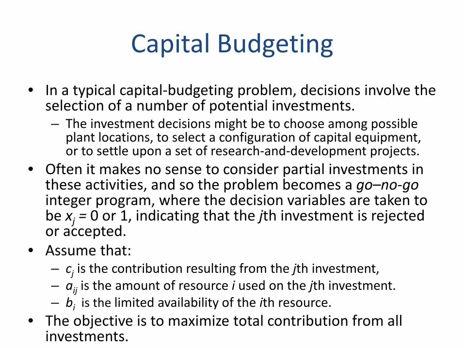
Capital Budgeting • In a typical capital-budgeting problem, decisions involve the

selection of a number of potential investments. – The investment decisions might be to choose among possible

plant locations, to select a configuration of capital equipment, or to settle upon a set of research-and-development projects.

• Often it makes no sense to consider partial investments in these activities, and so the problem becomes a go–no-go integer program, where the decision variables are taken to be xj = 0 or 1, indicating that the jth investment is rejected or accepted.

• Assume that: – cj is the contribution resulting from the jth investment, – aij is the amount of resource i used on the jth investment. – bi is the limited availability of the ith resource.

• The objective is to maximize total contribution from all investments.

Model

Note that…

• The coefficients aij represent the net cash flow from investment j in period i. – If the investment requires additional cash in period i ,

then aij > 0, – If the investment generates cash in period i,

then aij < 0. • The righthand-side coefficients bi represent the

incremental exogenous cash flows. – If additional funds are made available in period i,

then bi > 0, – If funds are withdrawn in period i ,

then bi < 0.

The capital-budgeting model can be made much richer by including logical

considerations

• The investment in a new product line is contingent upon previous investment in a new plant (contingency constraints)

• Conflicting projects (multiple-choice constraints)

The 0-1 knapsack problem

• A capital budgeting problem with a single resource:

Warehouse Location

• In modeling distribution systems, decisions must be made about tradeoffs between transportation costs and costs for operating distribution centers.

• As an example, suppose that a manager must decide which of n warehouses to use for meeting the demands of m customers for a good.

• The decisions to be made are which warehouses to operate and how much to ship from any warehouse to any customer.

Decision variables and relevant data

• There are two types of constraints for the model: – the demand dj of each customer must be filled from the

warehouses, – goods can be shipped from a warehouse only if it is

opened.

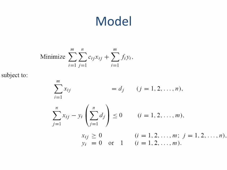
Model

Scheduling

• Consider the scheduling of airline flight personnel.

• The airline has a number of routing ‘‘legs’’ to be flown, such as 10 A.M. New York to Chicago, or 6 P.M.Chicago to Los Angeles.

• The airline must schedule its personnel crews on routes to cover these flights. One crew, for example, might be scheduled to fly a route containing the two legs just mentioned.

Decision variables and relevant data

• The coefficients aij define the acceptable combinations of legs and routes, taking into account such characteristics as sequencing of legs for making connections between flights and for including in the routes ground time for maintenance.

Model

An alternative formulation that permits a crew to ride as passengers

on a leg

• Set-partitioning:

• Set-covering

Traveling salesperson problem

• Starting from his home, a salesperson wishes to visit each of (n −1) other cities and return home at minimal cost.

• (S)He must visit each city exactly once and it costs cij to travel from city i to city j.

• What route should (s)he select?

Decision variables

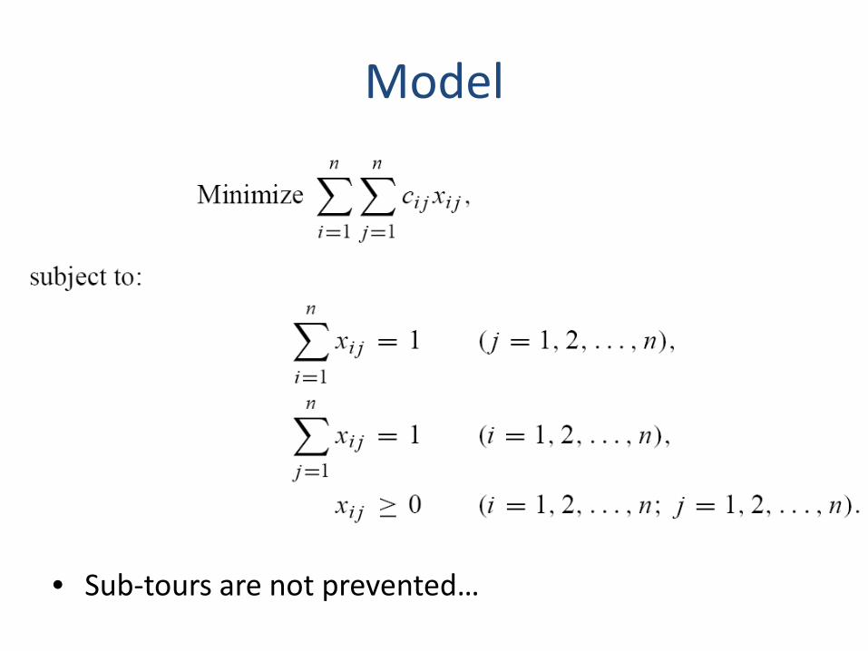
Model

• Sub-tours are not prevented…

Sub-tours elimination

• With n cities, (2n −1) constraints of this nature must be added… – True for this strategy and many other strategies used to

eliminate sub-tours in TSP models.

+

FORMULATING INTEGER PROGRAMS

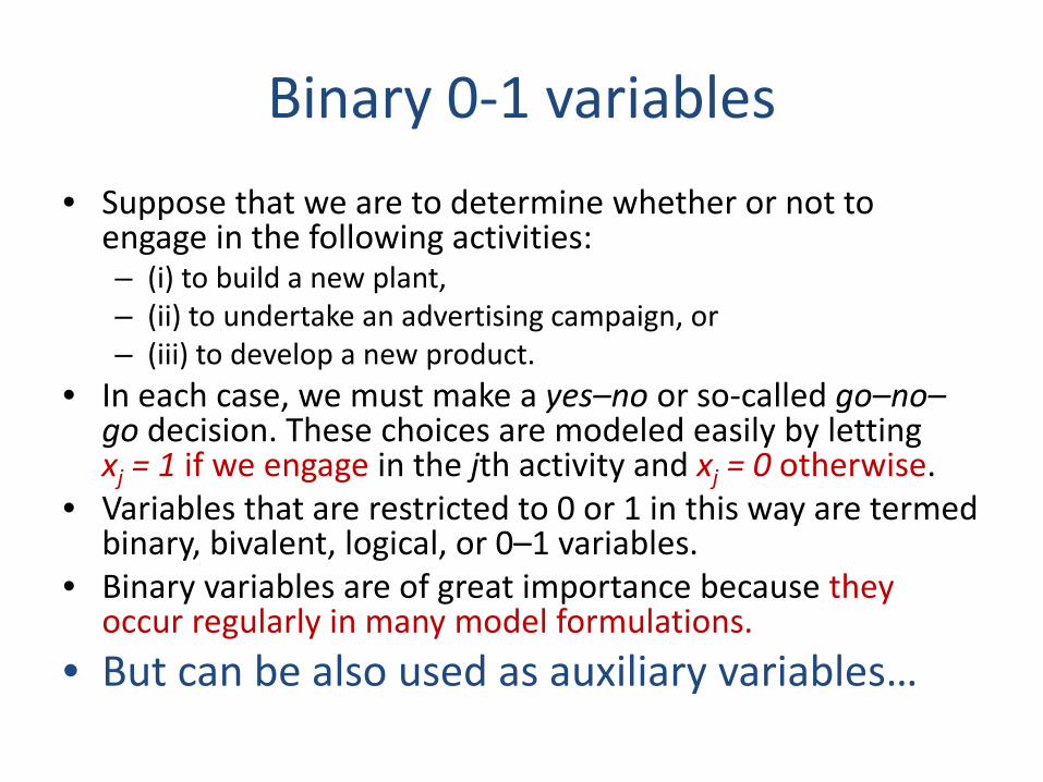
Binary 0-1 variables • Suppose that we are to determine whether or not to

engage in the following activities: – (i) to build a new plant, – (ii) to undertake an advertising campaign, or – (iii) to develop a new product.

• In each case, we must make a yes–no or so-called go–no–go decision. These choices are modeled easily by letting xj = 1 if we engage in the jth activity and xj = 0 otherwise.

• Variables that are restricted to 0 or 1 in this way are termed binary, bivalent, logical, or 0–1 variables.

• Binary variables are of great importance because they occur regularly in many model formulations.

• But can be also used as auxiliary variables…

Constraint Feasibility

• Does a given choice of the decision variables satisfies the constraint ?

Introduce a binary variable y with the interpretation:

and write B is chosen to be large enough so

that the constraint always is satisfied

if y = 1

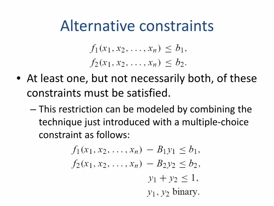
Alternative constraints

• At least one, but not necessarily both, of these constraints must be satisfied. – This restriction can be modeled by combining the

technique just introduced with a multiple-choice constraint as follows:

• We can save one integer variable in this formulation:

Conditional Constraints

• These constraints have the form:

• If we note that: (p ⇒ q) ⇔ (∼p ∨ q)

we end up with the following alternative constraints:

k-Fold Alternatives

• We must satisfy at least k of the constraints:

Assuming that Bj for j = 1, 2, . . . , p, are chosen so that the ignored constraints will not be binding, the general problem can be formulated as follows:

Compound Alternatives

Representing Nonlinear Functions

• Nonlinear functions can be represented by integer-programming formulations…

Fixed Costs • Frequently, the objective function for a minimization problem

contains fixed costs (preliminary design costs, fixed investment costs, fixed contracts, and so forth).

• Assume that the equipment has a capacity of B units. • Define y to be a binary variable that indicates when

the fixed cost is incurred, so that y = 1 when x > 0 and y = 0 when x = 0.

• Then the contribution to cost due to x may be written as

with the constraints

Piecewise Linear Representation

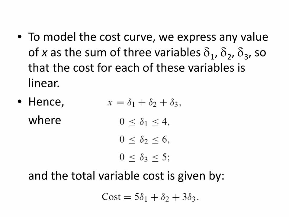
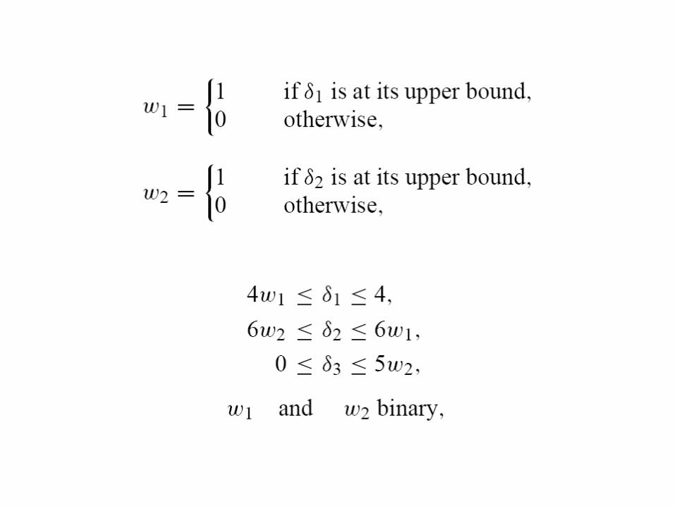
• To model the cost curve, we express any value of x as the sum of three variables δ1, δ2, δ3, so that the cost for each of these variables is linear.

• Hence, where and the total variable cost is given by:

• Note that we have defined the variables so that: – δ1 corresponds to the amount by which x exceeds 0,

but is less than or equal to 4; – δ2 is the amount by which x exceeds 4, but is less than

or equal to 10; and – δ3 is the amount by which x exceeds 10, but is less

than or equal to 15. • If this interpretation is to be valid, we must also

require that δ1 = 4 whenever δ2 > 0 and that δ2 = 6 whenever δ3 > 0.

• However, these restrictions on the variables are simply conditional constraints and can be modeled by introducing (more) binary variables:

Diseconomies of Scale • When marginal costs are increasing for a minimization

problem or marginal returns are decreasing for a maximization problem.

subject to: • The conditional constraints involving binary variables

in the previous formulation can be ignored if the cost curve appears in a minimization objective function, since the coefficients of δ1, δ2, δ3 imply that it is always best to set δ1 = 4 before taking δ2 > 0, and to set δ2 = 6 before taking δ3 > 0.

• This representation without integer variables is not valid, however, if economies of scale are present.

SOME CHARACTERISTICS OF INTEGER PROGRAMS

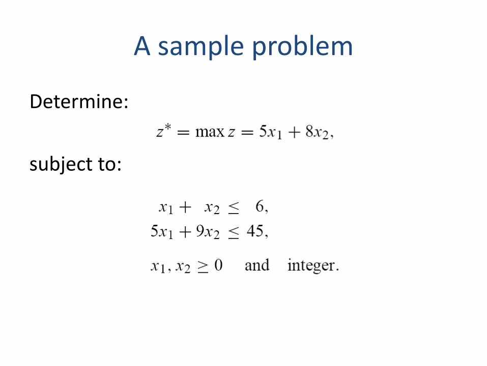
A sample problem

Determine: subject to:

Feasible region

Dots in the shaded region are feasible integer points.

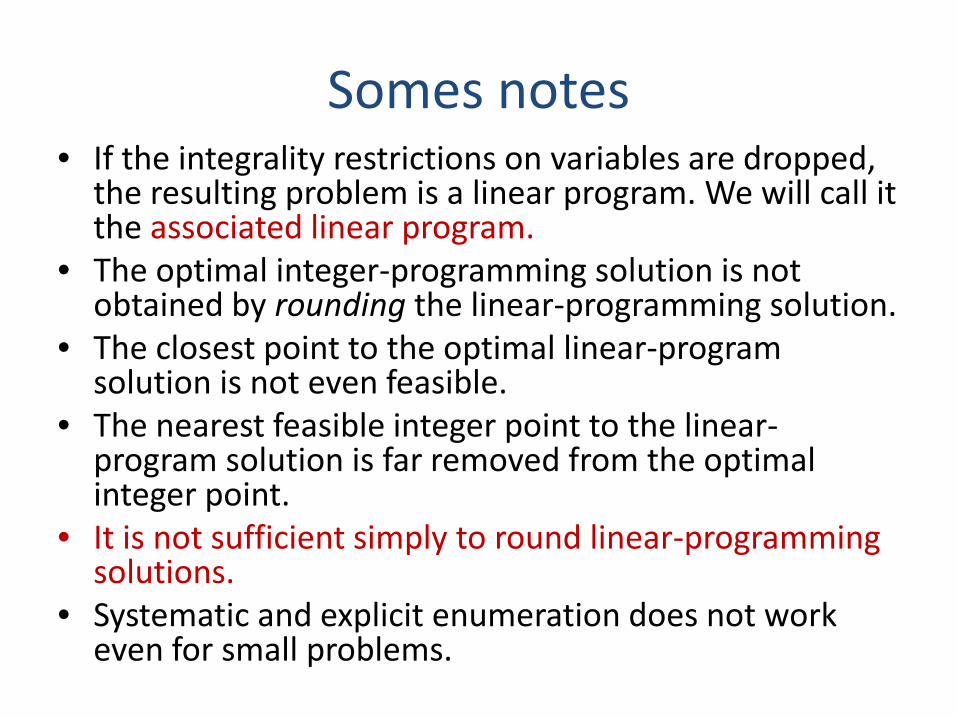
Somes notes • If the integrality restrictions on variables are dropped,

the resulting problem is a linear program. We will call it the associated linear program.

• The optimal integer-programming solution is not obtained by rounding the linear-programming solution.

• The closest point to the optimal linear-program solution is not even feasible.

• The nearest feasible integer point to the linear-program solution is far removed from the optimal integer point.

• It is not sufficient simply to round linear-programming solutions.

• Systematic and explicit enumeration does not work even for small problems.

BRANCH-AND-BOUND

Strategy of ‘‘divide and conquer’’ • An integer linear program is a linear program further

constrained by the integrality restrictions. • Thus, in a maximization problem, the value of the

objective function, at the linear-program optimum, will always be an upper bound on the optimal integer-programming objective.

• In addition, any integer feasible point is always a lower bound on the optimal linear-program objective value.

• The idea of branch-and-bound is to utilize these observations to systematically subdivide the linear programming feasible region and make assessments of the integer-programming problem based upon these subdivisions.

Further Considerations

• There are three points that have yet to be considered with respect to the branch-and-bound procedure: i. Can the linear programs corresponding to the

subdivisions be solved efficiently? ii. What is the best way to subdivide a given region,

and which unanalyzed subdivision should be considered next?

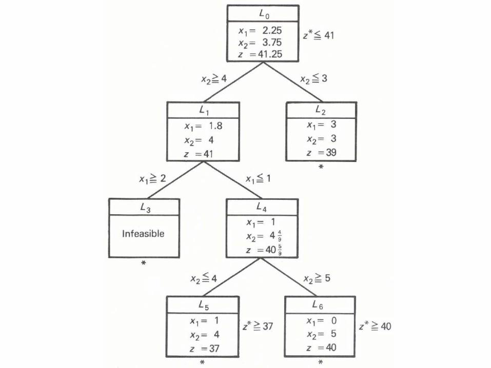
iii. Can the upper bound (z = 41, in the example) on the optimal value z of the integer program be improved while the problem is being solved?

Can the linear programs corresponding to the subdivisions be solved efficiently?

• Dual simplex method! – Adding the new constraint:

– Results in:

• We must pivot to isolate x2 in the second constraint and re-express the system as:

and perform a dual simplex method iteration.

What is the best way to subdivide a given region, and which unanalyzed subdivision

should be considered next? • If we can make our choice of subdivisions in such a way

as to rapidly obtain a good (with luck, near-optimal) integer solution z’, then we can eliminate many potential subdivisions immediately – as if any region has its linear programming value z < z’,

then the objective value of no integer point in that region can exceed z’ and the region need not be subdivided.

• There is no universal method for making the required choice, although several heuristic procedures have been suggested, such as selecting the subdivision: – with the largest optimal linear-programming value. – on a last-generated–first-analyzed basis (depth-first).

• Rules for determining which fractional variables to use in constructing subdivisions are more subtle…

Can the upper bound on the optimal value z* of the integer program be improved

while the problem is being solved?

• Initial upper bound = 41.25 41 if we recall that

the objective function coefficients are also integer.

• Current upper bound = 40 5/9 40, for the same

reasons.

Summary

• The essential idea of branch-and-bound is to subdivide the feasible region to develop bounds zL < z* < zU on z*.

• For a maximization problem, the lower bound zL is the highest value of any feasible integer point encountered.

• The upper bound is given by the optimal value of the associated linear program or by the largest value for the objective function at any ‘‘hanging’’ box.

• After considering a subdivision, we must branch to (move to) another subdivision and analyze it.

Summary

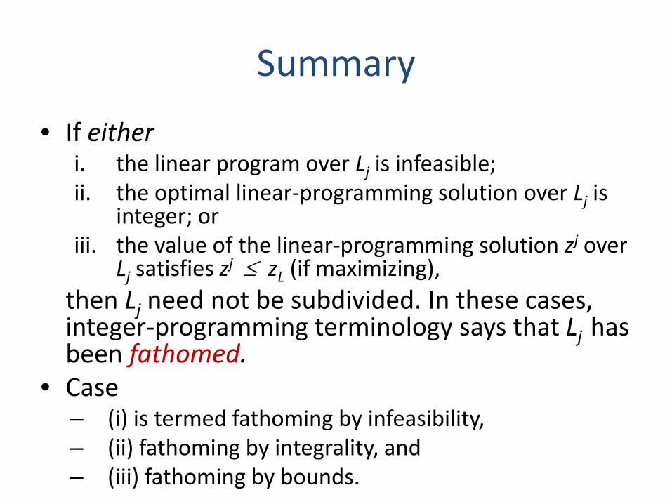
• If either i. the linear program over Lj is infeasible; ii. the optimal linear-programming solution over Lj is

integer; or iii. the value of the linear-programming solution zj over

Lj satisfies zj ≤ zL (if maximizing), then Lj need not be subdivided. In these cases,

integer-programming terminology says that Lj has been fathomed.

• Case – (i) is termed fathoming by infeasibility, – (ii) fathoming by integrality, and – (iii) fathoming by bounds.

Branch-and-bound flowchart

BRANCH-AND-BOUND FOR MIXED-INTEGER PROGRAMS

Branch-and-Bound for Mixed-Integer Programs

• The branch-and-bound approach just described is easily extended to solve problems in which some, but not all, variables are constrained to be integral.

• Subdivisions then are generated solely by the integral variables.

• In every other way, the procedure is the same as that specified above.

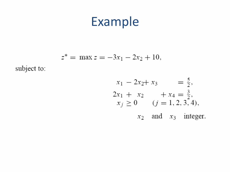
Example

Search Tree

Simplex tableaus

Simplex tableaus

BINARY BRANCH-AND-BOUND Implicit enumeration

A special branch-and-bound procedure for integer programs with only binary variables • The algorithm has the advantage that it

requires no linear-programming solutions. • In the ordinary branch-and-bound procedure,

subdivisions were analyzed by maintaining the linear constraints and dropping the integrality restrictions – relax the variables

• Here, we adopt the opposite tactic of always maintaining the 0–1 restrictions, but ignoring the linear inequalities – relax the constraints

General idea

• The idea is to utilize a branch-and-bound (or subdivision) process to fix some of the variables at 0 or 1.

• The variables remaining to be specified are called free variables.

• Note that, when the inequality constraints are ignored, the objective function is maximized by setting the free variables to zero, since their objective function coefficients are negative. – This is mandatory to apply this algorithm.

Example

subject to:

all coefficients are negative maximization problem

constraints are specified as ‘‘less than or equal to’’ inequalities

• We start with no fixed variables, and consequently every variable is free and set to zero.

• The solution does not satisfy the inequality constraints, and we must subdivide to search for feasible solutions.

• One subdivision choice might be: – For subdivision 1 : x1 = 1, – For subdivision 2 : x1 = 0.

• Now variable x1 is fixed in each subdivision. If the inequalities are ignored, the optimal solution over each subdivision has x2 = x3 = x4 = x5 = 0.

• The resulting solution in subdivision 1 gives z = – 8(1) – 2(0) – 4(0) – 5(0) + 10 = 2

and happens to satisfy the inequalities, so the optimal solution to the original problem is at least 2, z* ≥ 2.

• Also, subdivision 1 has been fathomed: – The above solution is best among all 0–1 combinations

with x1 = 1. – No other feasible 0–1 combination in subdivision 1 needs

to be evaluated explicitly. – These combinations have been considered implicitly.

• The solution with x2 = x3 = x4 = x5 = 0 in subdivision 2 is the same as the original solution with every variable at zero, and is infeasible.

• Consequently, the region must be subdivided further, say with x2 = 1 or x2 = 0, giving: – For subdivision 3 : x1 = 0, x2 = 1; – For subdivision 4 : x1 = 0, x2 = 0.

Enumeration tree to this point

• Completing it…

Complete tree

Note that

1. At , the solution x1 = 0, x2 = x3 = 1 , with free variables x4 = x5 = 0, is feasible, with z = 4, thus providing an improved lower bound on z.

2. At , the solution x1 = x3 = 0, x2 = x4 = 1, and free variable x5 = 0, has z = 1 < 4, so that no solution in that subdivision can be as good as that generated at .

3. At and , every free variable is fixed. In each case, the subdivisions contain only a single point, which is infeasible, and further subdivision is not possible.

Note that

4. At , the second inequality (with fixed variables x1 = x2 = 0) reads:

−2 x3 − x4 + x5 ≤ −4. No 0–1 values of x3, x4, or x5 ‘‘completing’’

the fixed variables x1 = x2 = 0 satisfy this constraint, since the lowest value for the lefthand side of this equation is −3 when x3 = x4 = 1 and x5 = 0.

The subdivision then has no feasible solution and need not be analyzed further.

Generalizing

• Subdivisions are fathomed if any of three conditions hold: i. the integer program is known to be infeasible over

the subdivision, for example, by the previous infeasibility test;

ii. the 0–1 solution obtained by setting free variables to zero satisfies the linear inequalities; or

iii. the objective value obtained by setting free variables to zero is no larger than the best feasible 0–1 solution previously generated.

Once again

• This algorithm is designed for problems in which: 1. the objective is a maximization with all

coefficients negative; and 2. constraints are specified as ‘‘less than or equal

to’’ inequalities.

• If not, then…

Problem transformation

• Minimization problems are transformed to maximization by multiplying cost coefficients by −1.

• If xj appears in the maximization form with a positive coefficient, then the variable substitution xj = 1− x’j everywhere in the model leaves the binary variable x’j with a negative objective-function coefficient.

• ‘‘Greater than or equal to’’ constraints can be multiplied by −1 to become ‘‘less than or equal to’’ constraints.