Embed Size (px)
Citation preview
058:0160 Chapter 8
Professor Fred Stern Fall 2019 1
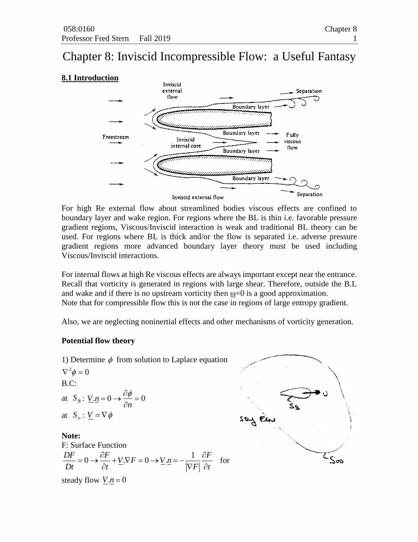
Chapter 8: Inviscid Incompressible Flow: a Useful Fantasy
8.1 Introduction
For high Re external flow about streamlined bodies viscous effects are confined to
boundary layer and wake region. For regions where the BL is thin i.e. favorable pressure
gradient regions, Viscous/Inviscid interaction is weak and traditional BL theory can be
used. For regions where BL is thick and/or the flow is separated i.e. adverse pressure
gradient regions more advanced boundary layer theory must be used including
Viscous/Inviscid interactions.
For internal flows at high Re viscous effects are always important except near the entrance.
Recall that vorticity is generated in regions with large shear. Therefore, outside the B.L
and wake and if there is no upstream vorticity then ω=0 is a good approximation.
Note that for compressible flow this is not the case in regions of large entropy gradient.
Also, we are neglecting noninertial effects and other mechanisms of vorticity generation.
Potential flow theory
1) Determine from solution to Laplace equation
02
B.C:
at BS : . 0 0V nn
at S : V
Note:
F: Surface Function
10 . 0 .
DF F FV F V n
Dt t F t
for
steady flow . 0V n
058:0160 Chapter 8
Professor Fred Stern Fall 2019 2
2) Determine V from V and p(x) from Bernoulli equation
Therefore, primarily for external flow application we now consider inviscid flow theory (
0 ) and incompressible flow ( const )
Euler equation:
. 0
. ( )
V
DVp g
Dt
VV V p z
t
2
.2
: 2
VV V V
Where V vorticity fluid angular velocity
21( )
2
0 0 :
Vp V z V
t
If ie V then V
1( )
2p z B t
t
Continuity equation shows that GDE for is the Laplace equation which is a 2nd order
linear PDE ie superposition principle is valid. (Linear combination of solution is also a
solution) 2
1 2
2
2 2 2 2 1
1 2 1 2 2
2
0
00 ( ) 0 0
0
V
Techniques for solving Laplace equation:
1) superposition of elementary solution (simple geometries)
2) surface singularity method (integral equation)
3) FD or FE
4) electrical or mechanical analogs
5) Conformal mapping ( for 2D flow)
6) Analytical for simple geometries (separation of variable etc)
058:0160 Chapter 8
Professor Fred Stern Fall 2019 3
8.2 Elementary plane-flow solutions:
Recall that for 2D we can define a stream function such that:
x
y
v
u
0)()( 2
yxyxz
yxuv
i.e. 02
Also recall that and are orthogonal.
yx
xy
v
u
udyvdxdydxd
vdyudxdydxd
yx
yx
i.e.
const
const
dx
dyv
u
dx
dy
1
Uniform stream
yx
xy
v
constUu
0
i.e. yU
xU
Note: 022 is satisfied.
ˆV U i
Say a uniform stream is at an angle to
the x-axis:
cosu Uy x
sinv Ux y
058:0160 Chapter 8
Professor Fred Stern Fall 2019 4
After integration, we obtain the following expressions for the stream function and velocity
potential:
cos sinU y x
cos sinU x y
2D Source or Sink:
𝑥 = 𝑟 cos 𝜃
𝑦 = 𝑟 sin 𝜃
Imagine that fluid comes out radially at origin with uniform rate in all directions.
(singularity at origin where velocity is infinite)
Consider a circle of radius r enclosing this source. Let vr be the radial component of
velocity associated with this source (or sink). Then, from conservation of mass, for a
cylinder of radius r, and width b, perpendicular to the paper, 3
A
LQ V d A
S
where 𝑉 = 𝑣𝑟𝑒�̂�; 𝑛 = 𝑒�̂�; 𝑑𝐴 = 𝑟𝑑𝜃𝑏
2
,
2
r
r
Q r b v
Or
Qv
br
0, vr
mvr
Where: 2
Qm
b is the source strength with unit m2/s velocity × length
(m>0 for source and m<0 for sink). Note that V is singular at (0,0) since rv
In a polar coordinate system, for 2-D flows we will use:
𝑉 = 𝛻𝜙 =𝜕𝜙
𝜕𝑟𝑒�̂� +
1
𝑟
𝜕𝜙
𝜕𝜃𝑒�̂�
𝛻 =𝜕
𝜕𝑟𝑒�̂� +
1
𝑟
𝜕
𝜕𝜃𝑒�̂�
058:0160 Chapter 8
Professor Fred Stern Fall 2019 5
And:
. 0
1 1( ) ( ) 0r
V
rv vr r r
i.e.:
rv
rrvr
r
1 velocityTangential
1 velocityRadial
Such that 0V by definition.
Therefore,
rv
rrvr
r
10
1
r
m
i.e.
x
ymm
yxmrm
1
22
tan
lnln
Doublets:
The doublet is defined as:
𝛹 = −𝑚
2𝜋 ( 𝜃1⏟
𝑠𝑖𝑛𝑘
− 𝜃2⏟𝑠𝑜𝑢𝑟𝑐𝑒
) → 𝜃1 − 𝜃2 = −2𝜋𝛹
𝑚
𝑡𝑎𝑛 (−2𝜋𝛹
𝑚) = 𝑡𝑎𝑛(𝜃1 − 𝜃2) =
𝑡𝑎𝑛 𝜃1 − 𝑡𝑎𝑛 𝜃2
1 + 𝑡𝑎𝑛 𝜃1 𝑡𝑎𝑛 𝜃2
𝑡𝑎𝑛 𝜃1 =𝑟 𝑠𝑖𝑛 𝜃
𝑟 𝑐𝑜𝑠 𝜃 − 𝑎; 𝑡𝑎𝑛 𝜃2 =
𝑟 𝑠𝑖𝑛 𝜃
𝑟 𝑐𝑜𝑠 𝜃 + 𝑎
𝑡𝑎𝑛 (−2𝜋𝛹
𝑚) =
2𝑎𝑟 sin 𝜃
𝑟2 − 𝑎2
058:0160 Chapter 8
Professor Fred Stern Fall 2019 6
Therefore
Ψ = −𝑚
2𝜋tan−1 (
2𝑎𝑟 sin 𝜃
𝑟2 − 𝑎2)
For small distance
Ψ = −𝑚
2𝜋
2𝑎𝑟 sin 𝜃
𝑟2 − 𝑎2=
𝑚𝑎𝑟 sin 𝜃
𝜋(𝑟2 − 𝑎2)
The doublet is formed by letting 𝑎 → 0 while increasing the strength m (𝑚 → ∞) so that
doublet strength 𝐾 =𝑚𝑎
𝜋 remains constant
Ψ = −𝐾 sin 𝜃
𝑟
Corresponding potential
𝜙 =𝐾 cos 𝜃
𝑟
By rearranging
Ψ = −𝐾 rsin 𝜃
𝑟2= −
𝐾𝑦
𝑥2 + 𝑦2→ 𝑥2 + (𝑦 +
𝐾
2Ψ)
2
= (𝐾
2Ψ)
2
= 𝑅2
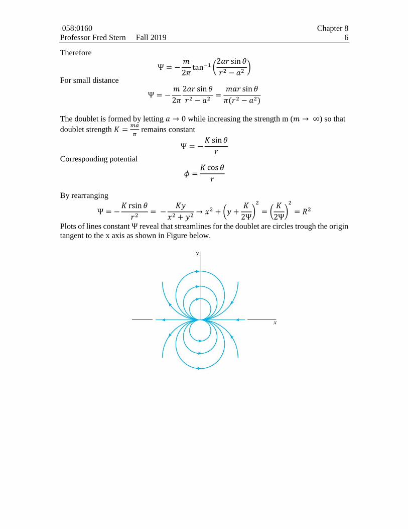
Plots of lines constant Ψ reveal that streamlines for the doublet are circles trough the origin
tangent to the x axis as shown in Figure below.
058:0160 Chapter 8
Professor Fred Stern Fall 2019 7
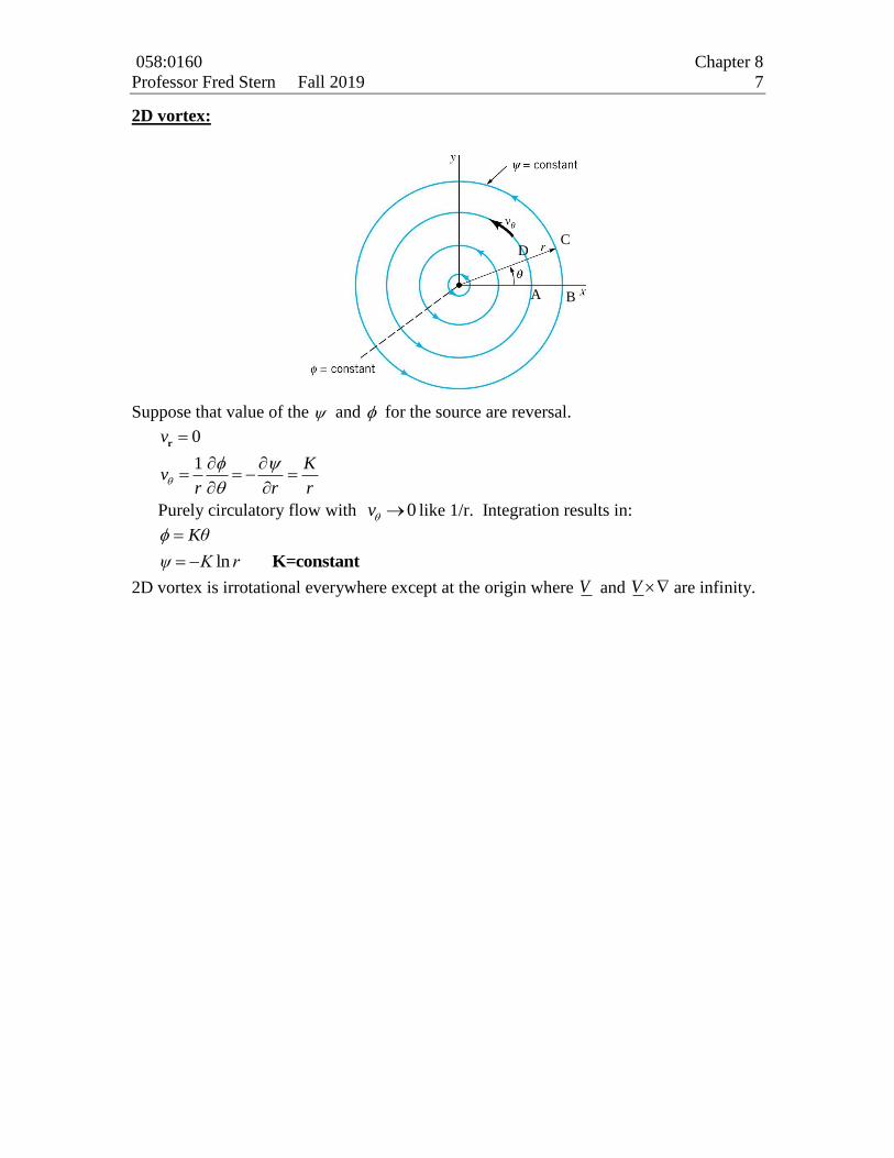
2D vortex:
Suppose that value of the and for the source are reversal.
0
1
rv
Kv
r r r
Purely circulatory flow with 0v like 1/r. Integration results in:
ln K=constant
Kθ
ψ K r
2D vortex is irrotational everywhere except at the origin where V and V are infinity.
A B
C D
058:0160 Chapter 8
Professor Fred Stern Fall 2019 8
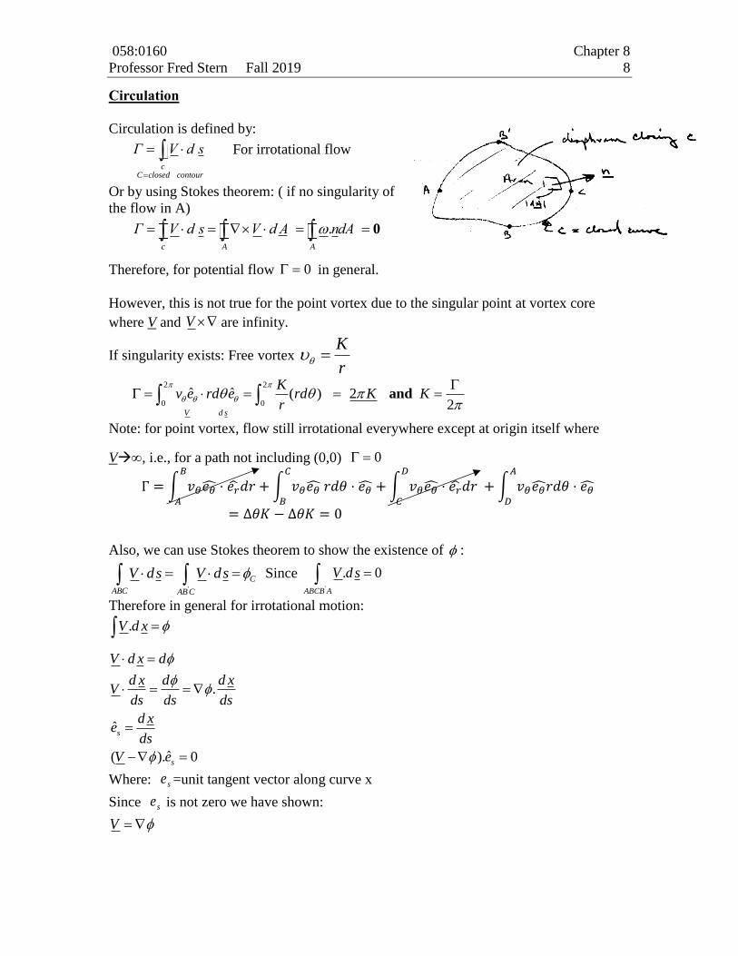
Circulation
Circulation is defined by:
cC closed contour
Γ V d s
For irrotational flow
Or by using Stokes theorem: ( if no singularity of
the flow in A)
. 0c A A
Γ V d s V d A ndA
Therefore, for potential flow 0 in general.
However, this is not true for the point vortex due to the singular point at vortex core
where V and V are infinity.
If singularity exists: Free vortex r
K
2 2
0 0ˆ ˆ ( ) 2
2 and
V d s
Kv e rd e rd K K
r
Note: for point vortex, flow still irrotational everywhere except at origin itself where
V, i.e., for a path not including (0,0) 0
Γ = ∫ 𝑣𝜃𝑒�̂� ⋅ 𝑒�̂�𝑑𝑟𝐵
𝐴
+ ∫ 𝑣𝜃𝑒�̂� 𝑟𝑑𝜃 ⋅ 𝑒�̂�
𝐶
𝐵
+ ∫ 𝑣𝜃𝑒�̂� ⋅ 𝑒�̂�𝑑𝑟 𝐷
𝐶
+ ∫ 𝑣𝜃𝑒�̂�𝑟𝑑𝜃 ⋅ 𝑒�̂� 𝐴
𝐷
= Δ𝜃𝐾 − Δ𝜃𝐾 = 0
Also, we can use Stokes theorem to show the existence of :
'
C
ABC AB C
V ds V ds Since '
. 0
ABCB A
V d s
Therefore in general for irrotational motion:
.V d x
Where: se =unit tangent vector along curve x
Since se is not zero we have shown:
V
.
ˆ
ˆ( ). 0
s
s
V d x d
d x d d xV
ds ds ds
d xe
ds
V e
058:0160 Chapter 8
Professor Fred Stern Fall 2019 9
i.e. velocity vector is gradient of a scalar function if the motion is irrotational. (
0V ds )
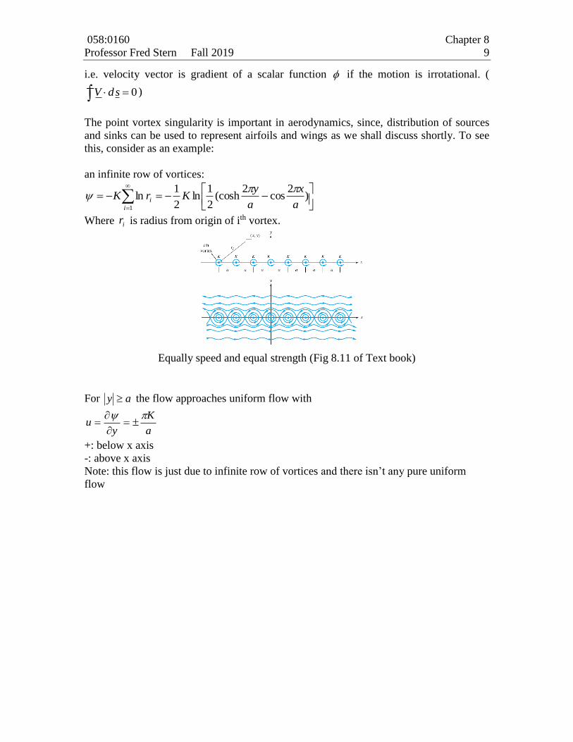
The point vortex singularity is important in aerodynamics, since, distribution of sources
and sinks can be used to represent airfoils and wings as we shall discuss shortly. To see
this, consider as an example:
an infinite row of vortices:
)2
cos2
(cosh2
1ln
2
1ln
1 a
x
a
yKrK
i
i
Where ir is radius from origin of ith vortex.
Equally speed and equal strength (Fig 8.11 of Text book)
For ay the flow approaches uniform flow with
a
K
yu
+: below x axis
-: above x axis
Note: this flow is just due to infinite row of vortices and there isn’t any pure uniform
flow
058:0160 Chapter 8
Professor Fred Stern Fall 2019 10
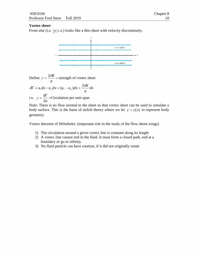
Vortex sheet:
From afar (i.e. ay ) looks like a thin sheet with velocity discontinuity.
Define a
K
2strength of vortex sheet
dxa
Kdxuudxudxud ulul
2)(
i.e. dx
d =Circulation per unit span
Note: There is no flow normal to the sheet so that vortex sheet can be used to simulate a
body surface. This is the basis of airfoil theory where we let )(x to represent body
geometry.
Vortex theorem of Helmholtz: (important role in the study of the flow about wings)
1) The circulation around a given vortex line is constant along its length
2) A vortex line cannot end in the fluid. It must form a closed path, end at a
boundary or go to infinity.
3) No fluid particle can have rotation, if it did not originally rotate
058:0160 Chapter 8
Professor Fred Stern Fall 2019 11
8.3 Potential Flow Solutions for Simple Geometries
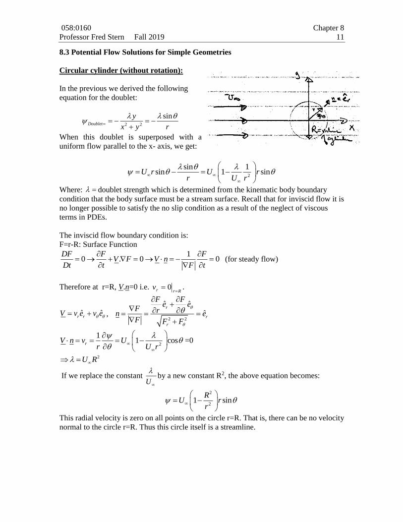
Circular cylinder (without rotation):
In the previous we derived the following
equation for the doublet:
2 2
sinDoublet
y
x y r
When this doublet is superposed with a
uniform flow parallel to the x- axis, we get:
2
sin 1sin 1 sinU r U r
r U r
Where: doublet strength which is determined from the kinematic body boundary
condition that the body surface must be a stream surface. Recall that for inviscid flow it is
no longer possible to satisfy the no slip condition as a result of the neglect of viscous
terms in PDEs.
The inviscid flow boundary condition is:
F=r-R: Surface Function
10 . 0 0
DF F FV F V n
Dt t F t
(for steady flow)
Therefore at r=R, V.n=0 i.e. Rrrv
0 .
ˆ ˆr rV v e v e ,
2 2
ˆ ˆ
ˆr
r
r
F Fe e
F rn eF F F
2
11 cosrV n v U
r U r
=0
2U R
If we replace the constant U
by a new constant R2, the above equation becomes:
2
21 sin
RU r
r
This radial velocity is zero on all points on the circle r=R. That is, there can be no velocity
normal to the circle r=R. Thus this circle itself is a streamline.
058:0160 Chapter 8
Professor Fred Stern Fall 2019 12
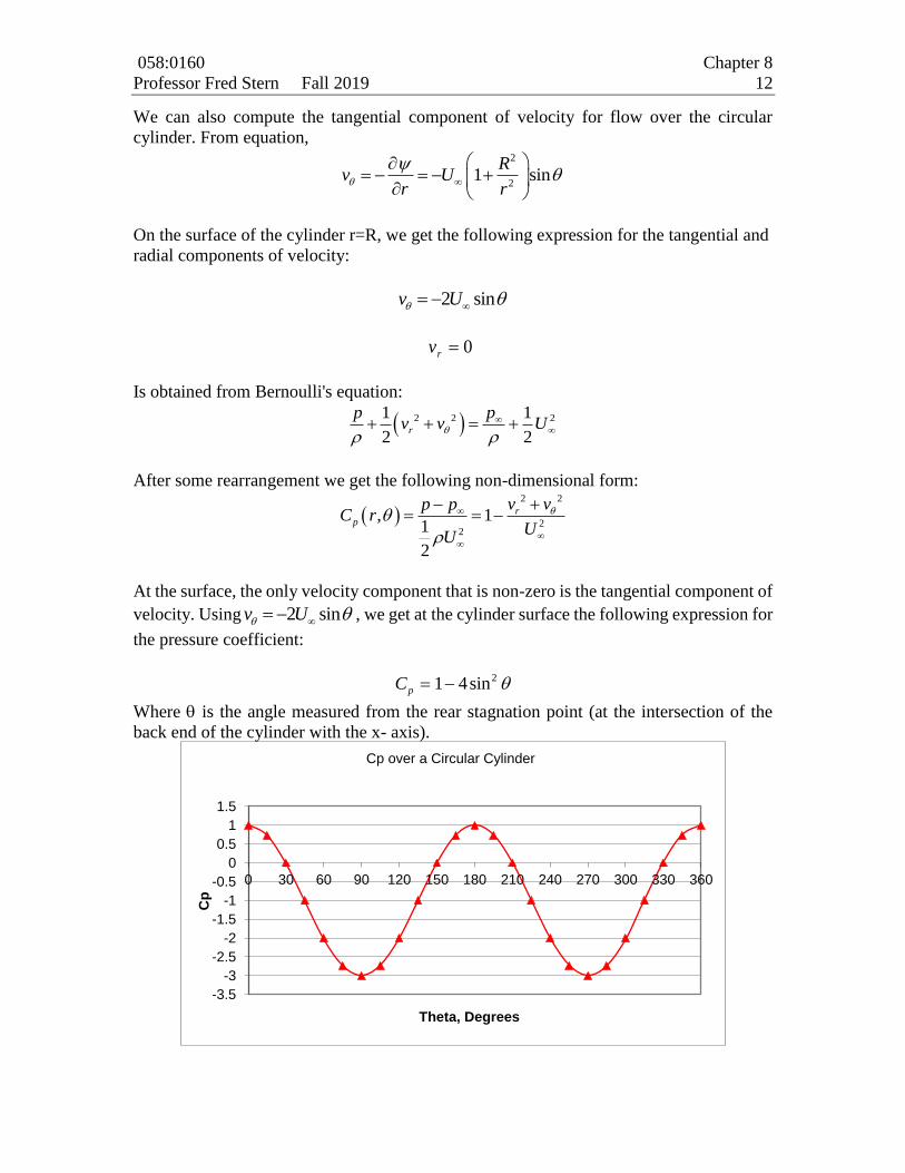
We can also compute the tangential component of velocity for flow over the circular
cylinder. From equation, 2
21 sin
Rv U
r r
On the surface of the cylinder r=R, we get the following expression for the tangential and
radial components of velocity:
2 sinv U
0rv
Is obtained from Bernoulli's equation:
2 2 21 1
2 2r
ppv v U
After some rearrangement we get the following non-dimensional form:
2 2
22
, 11
2
rp
v vp pC r
UU
At the surface, the only velocity component that is non-zero is the tangential component of
velocity. Using 2 sinv U , we get at the cylinder surface the following expression for
the pressure coefficient:
Where is the angle measured from the rear stagnation point (at the intersection of the
back end of the cylinder with the x- axis).
Cp 1 4 2sin
-3.5
-3
-2.5
-2
-1.5
-1
-0.5
0
0.5
1
1.5
0 30 60 90 120 150 180 210 240 270 300 330 360
Cp
Theta, Degrees
Cp over a Circular Cylinder
058:0160 Chapter 8
Professor Fred Stern Fall 2019 13
From pressure coefficient we can calculate the fluid force on the cylinder:
21( ) ( , )
2p
A A
F p p nds U C R nds
( )ds Rd b b=span length 2
2 2
0
1 ˆ ˆ(1 4sin )(cos sin )2
F U bR i j d
2 2
ˆ
1 1
2 2
L
Lift F jC
U bR U bR
= 0sin)sin41(
2
0
2
d (due to symmetry of flow
around x axis)
2 2
ˆ
1 1
2 2
F
Drag F iC
U bR U bR
= 0cos)sin41(
2
0
2
d (dÁlembert paradox)
D
058:0160 Chapter 8
Professor Fred Stern Fall 2019 14
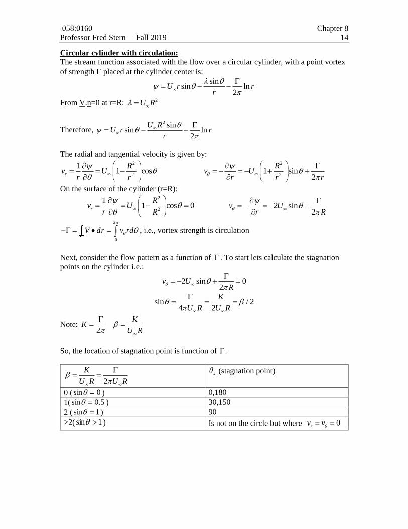
Circular cylinder with circulation:
The stream function associated with the flow over a circular cylinder, with a point vortex
of strength placed at the cylinder center is:
sinsin ln
2U r r
r
From V.n=0 at r=R: 2U R
Therefore, 2 sin
sin ln2
U RU r r
r
The radial and tangential velocity is given by: 2
2
11 cosr
Rv U
r r
2
21 sin
2
Rv U
r r r
On the surface of the cylinder (r=R):
2
2
11 cos 0r
Rv U
r R
2 sin
2v U
r R
2
0
V dr v rd
, i.e., vortex strength is circulation
Next, consider the flow pattern as a function of . To start lets calculate the stagnation
points on the cylinder i.e.:
2 sin 02
v UR
sin / 24 2
K
U R U R
Note: 2
KK
U R
So, the location of stagnation point is function of .
2
K
U R U R
s (stagnation point)
0 ( 0sin ) 0,180
1( 5.0sin ) 30,150
2 ( 1sin ) 90
>2( 1sin ) Is not on the circle but where 0rv v
058:0160 Chapter 8
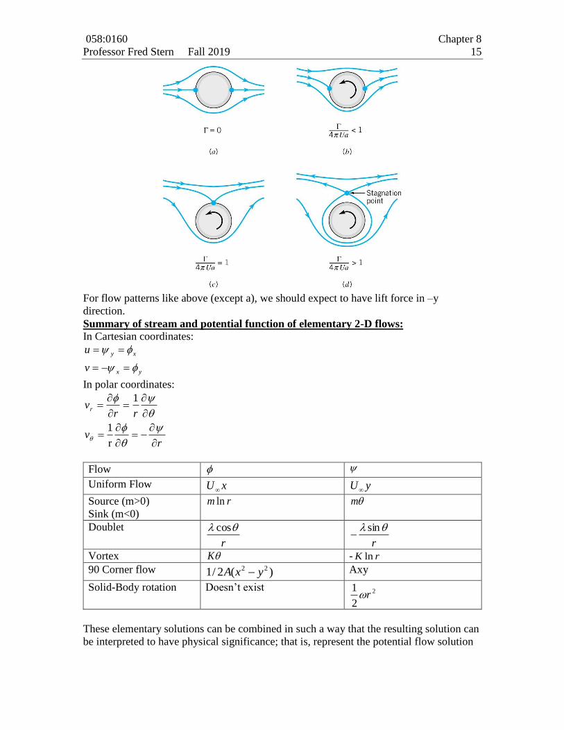
Professor Fred Stern Fall 2019 15
For flow patterns like above (except a), we should expect to have lift force in –y
direction.
Summary of stream and potential function of elementary 2-D flows:
In Cartesian coordinates:
yx
xy
v
u
In polar coordinates:
rv
rrvr
r
1
1
Flow
Uniform Flow xU yU
Source (m>0)
Sink (m<0)
lnm r m
Doublet
r
cos
r
sin
Vortex K - lnK r
90 Corner flow )(2/1 22 yxA Axy
Solid-Body rotation Doesn’t exist 2
2
1r
These elementary solutions can be combined in such a way that the resulting solution can
be interpreted to have physical significance; that is, represent the potential flow solution
058:0160 Chapter 8
Professor Fred Stern Fall 2019 16
for various geometries. Also, methods for arbitrary geometries combine uniform stream
with distribution of the elementary solution on the body surface.
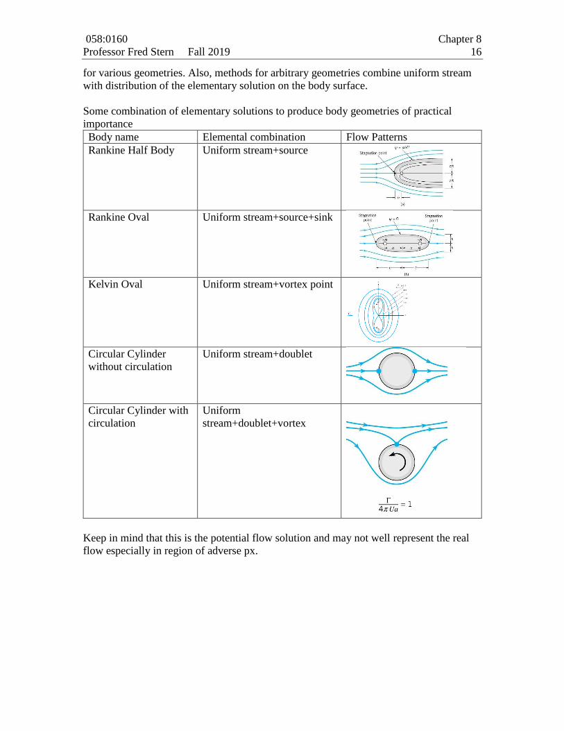
Some combination of elementary solutions to produce body geometries of practical
importance
Body name Elemental combination Flow Patterns
Rankine Half Body Uniform stream+source
Rankine Oval Uniform stream+source+sink
Kelvin Oval Uniform stream+vortex point
Circular Cylinder
without circulation
Uniform stream+doublet
Circular Cylinder with
circulation
Uniform
stream+doublet+vortex
Keep in mind that this is the potential flow solution and may not well represent the real
flow especially in region of adverse px.
058:0160 Chapter 8
Professor Fred Stern Fall 2019 17
The Kutta – Joukowski lift theorem:
Since we know the tangential component of velocity at any point on the cylinder (and the
radial component of velocity is zero), we can find the pressure field over the surface of
the cylinder from Bernoulli’s equation: 22 2
2 2 2
rvv p Up
Therefore:
2 2
2 2 2 2
2 2
2
1 12 sin 2 sin sin
2 2 2 8
sin sin
Up p U U p U U
R R R
A B C
where
2
2
2 2
1
2 8A p U
R
UB
R
22C U Calculation of Lift: Let us first consider lift. Lift per unit span, L (i.e. per unit distance
normal to the plane of the paper) is given by:
On the surface of the cylinder, x = Rcos. Thus, dx = -Rsind, and the above integrals
may be thought of as integrals with respect to . For the lower surface, varies between
and 2. For the upper surface, varies between and 0. Thus,
Reversing the upper and lower limits of the second integral, we get:
Substituting for B ,we get:
This is an important result. It says that clockwise vortices (negative numerical values of )
will produce positive lift that is proportional to and the free stream speed with direction
90 degrees from the stream direction rotating opposite to the circulation. Kutta and
Joukowski generalized this result to lifting flow over airfoils. Equation is
known as the Kutta-Joukowski theorem.
Lower upper
pdxpdxL
2 0
22 sinsinsinsinsinsin dCBARdCBARL
2
0
32
2
0
2 sinsinsinsinsinsin BRdCBARdCBARL
uL
uL
058:0160 Chapter 8
Professor Fred Stern Fall 2019 18
Drag: We can likewise integrate drag forces. The drag per unit span, D, is given by:
Since y=Rsin on the cylinder, dy=Rcosd. Thus, as in the case of lift, we can convert
these two integrals over y into integrals over . On the front side, varies from 3/2 to /2.
On the rear side, varies between 3/2 and /2. Performing the integration, we can show
that
This result is in contrast to reality, where drag is high due to viscous separation. This
contrast between potential flow theory and drag is the dÁlembert Paradox.
The explanation of this paradox are provided by Prandtl (1904) with his boundary layer
theory i.e. viscous effects are always important very close to the body where the no slip
boundary condition must be satisfied and large shear stress exists which contributes the
drag.
Front rear
pdypdyD
0D
058:0160 Chapter 8
Professor Fred Stern Fall 2019 19
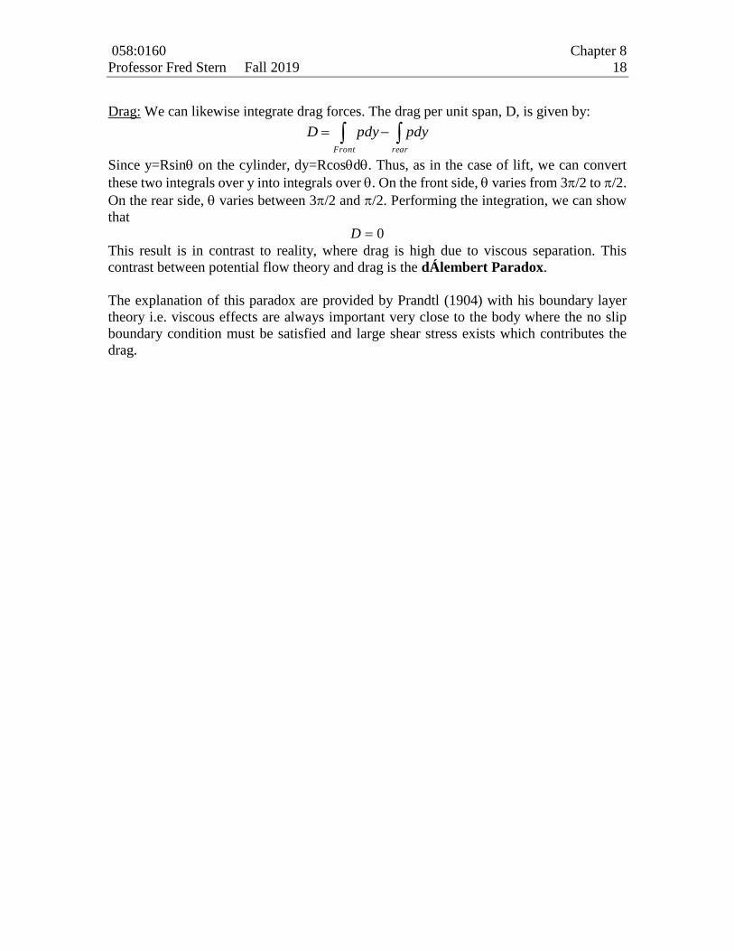
Lift for rotating Cylinder:
We know that L U therefore:
21(2 )
2
L
LC
U RU R
Define:
R
dvvAverage
2
1
2
12
0
Note: c c c
Γ V d s V d A V Rd
2averagfeLC v
U
Velocity ratio: a
U
Theoretical and experimental lift and drag of a rotating cylinder
Experiments have been performed that simulate the previous flow by rotating a circular
cylinder in a uniform stream. In this case Rv which is due to no slip boundary
condition.
- Lift is quite high but not as large as theory (due to viscous effect ie flow separation)
058:0160 Chapter 8
Professor Fred Stern Fall 2019 20
- Note drag force is also fairy high
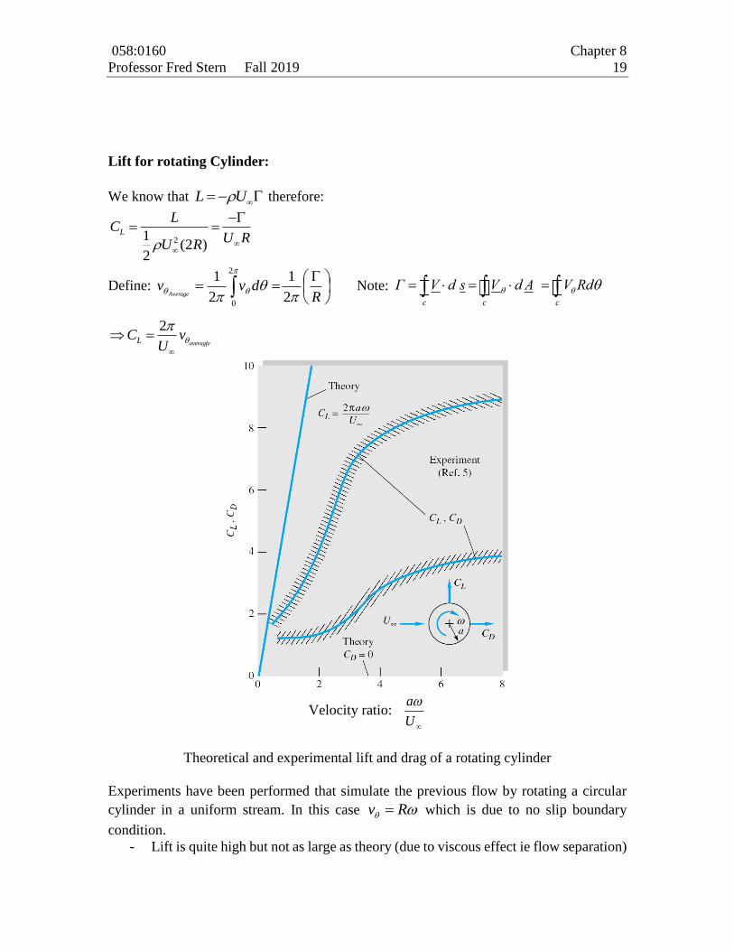
Flettner (1924) used rotating cylinder to produce forward motion.
058:0160 Chapter 8
Professor Fred Stern Fall 2019 21
058:0160 Chapter 8
Professor Fred Stern Fall 2019 22
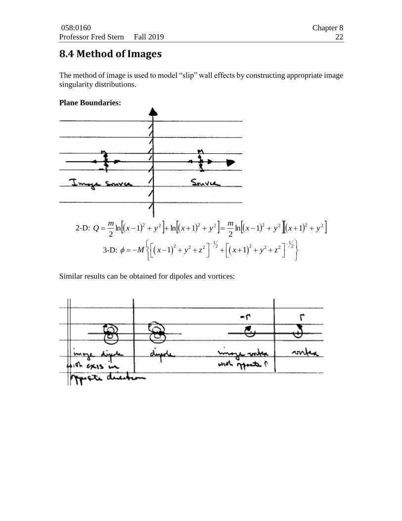
8.4 Method of Images
The method of image is used to model “slip” wall effects by constructing appropriate image
singularity distributions.
Plane Boundaries:
2-D: 2222222211ln
21ln1ln
2yxyx
myxyx
mQ
3-D: 1 1
2 22 22 2 2 21 1M x y z x y z
Similar results can be obtained for dipoles and vortices:
058:0160 Chapter 8
Professor Fred Stern Fall 2019 23
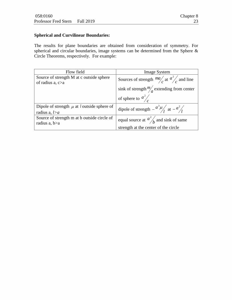
Spherical and Curvilinear Boundaries:
The results for plane boundaries are obtained from consideration of symmetry. For
spherical and circular boundaries, image systems can be determined from the Sphere &
Circle Theorems, respectively. For example:
Flow field Image System
Source of strength M at c outside sphere
of radius a, c>a Sources of strength
cma at
ca 2
and line
sink of strengtha
m extending from center
of sphere to c
a 2
Dipole of strength at l outside sphere of
radius a, l>a dipole of strength
la 3
at l
a 2
Source of strength m at b outside circle of
radius a, b>a equal source at
ba 2
and sink of same
strength at the center of the circle
058:0160 Chapter 8
Professor Fred Stern Fall 2019 24
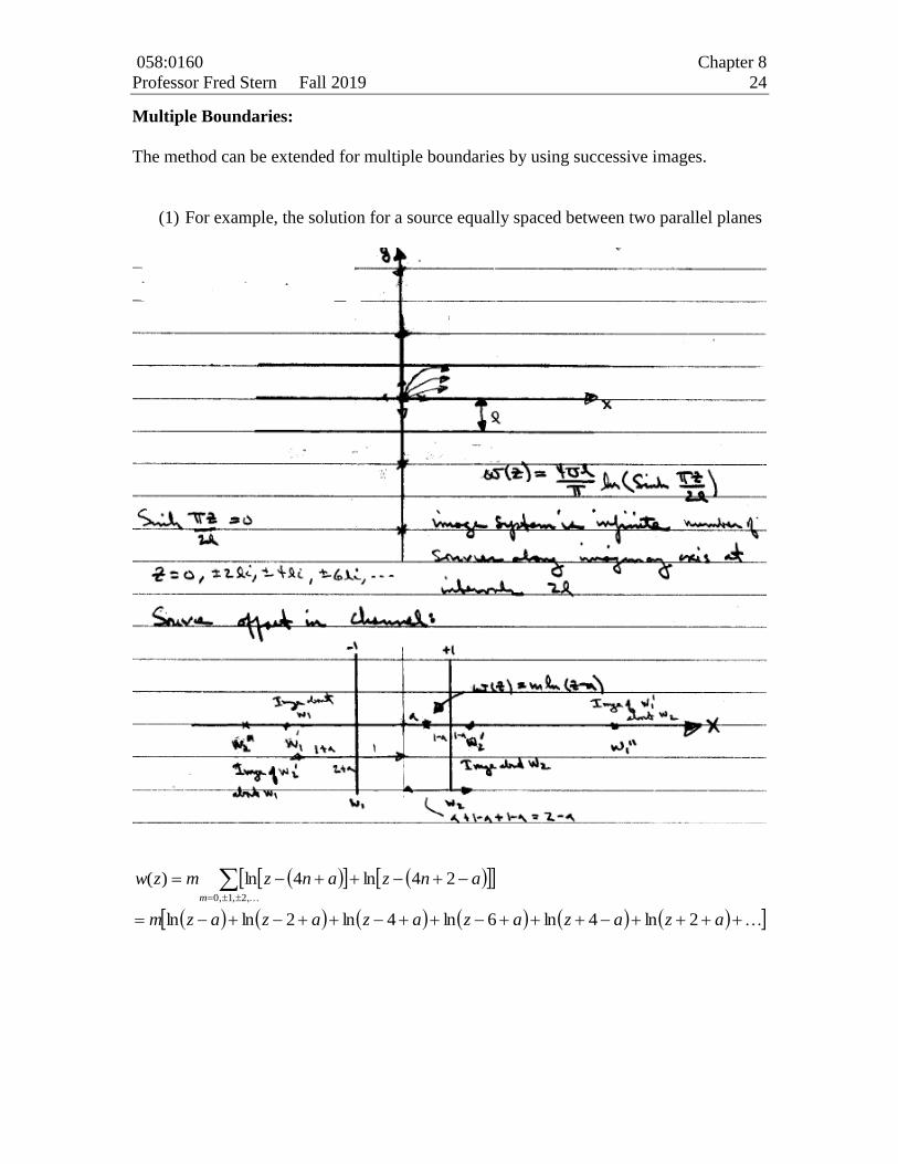
Multiple Boundaries:
The method can be extended for multiple boundaries by using successive images.
(1) For example, the solution for a source equally spaced between two parallel planes
azazazazazazm
anzanzmzwm
2ln4ln6ln4ln2lnln
24ln4ln)(,2,1,0
058:0160 Chapter 8
Professor Fred Stern Fall 2019 25
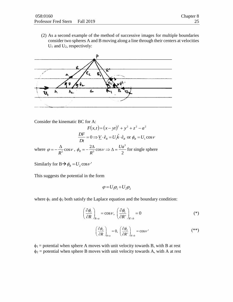
(2) As a second example of the method of successive images for multiple boundaries
consider two spheres A and B moving along a line through their centers at velocities
U1 and U2, respectively:
Consider the kinematic BC for A:
2222, azyytxtxF
1 1ˆˆ ˆ0 or cosR R R
DFV e U k e U
Dt
where 2
cosR
, 3
3
2cos
2R
Ua
R
for single sphere
Similarly for B 2 cos 'R U
This suggests the potential in the form
1 1 2 2U U
where 1 and 2 both satisfy the Laplace equation and the boundary condition:
1 1
'
cos , 0'R a R bR R
(*)
2 2
'
0, cos ''R a R bR R
(**)
1 = potential when sphere A moves with unit velocity towards B, with B at rest
2 = potential when sphere B moves with unit velocity towards A, with A at rest
058:0160 Chapter 8
Professor Fred Stern Fall 2019 26
If B were absent. 3
01 2 2
cos cos2
a
R R
,
2
3
0
a
but this does not satisfy the second condition in (*). To satisfy this, we introduce the image
of 0 in B, which is a doublet 1 directed along BA at A1, the inverse point of A with
respect to B. This image requires an image 2 at A2, the inverse of A1 with respect to A,
and so on. Thus we have an infinite series of images A1, A2, … of strengths 1 , 2 , 3 etc.
where the odd suffixes refer to points within B and the even to points within A.
Let &n nf AA AB c
c
bcf
2
1 , 1
2
2f
af ,
2
2
3fc
bcf
,…
3
3
01c
b,
3
1
3
12f
a,
3
2
3
23fc
b,…
where 1 = image dipole strength, 0 = dipole strength 3
3
sistance
radius
0 1 1 2 21 2 2 2
1 2
cos cos cos
R R R
with a similar development procedure for 2.
Although exact, this solution is of unwieldy form. Let’s investigate the possibility of an
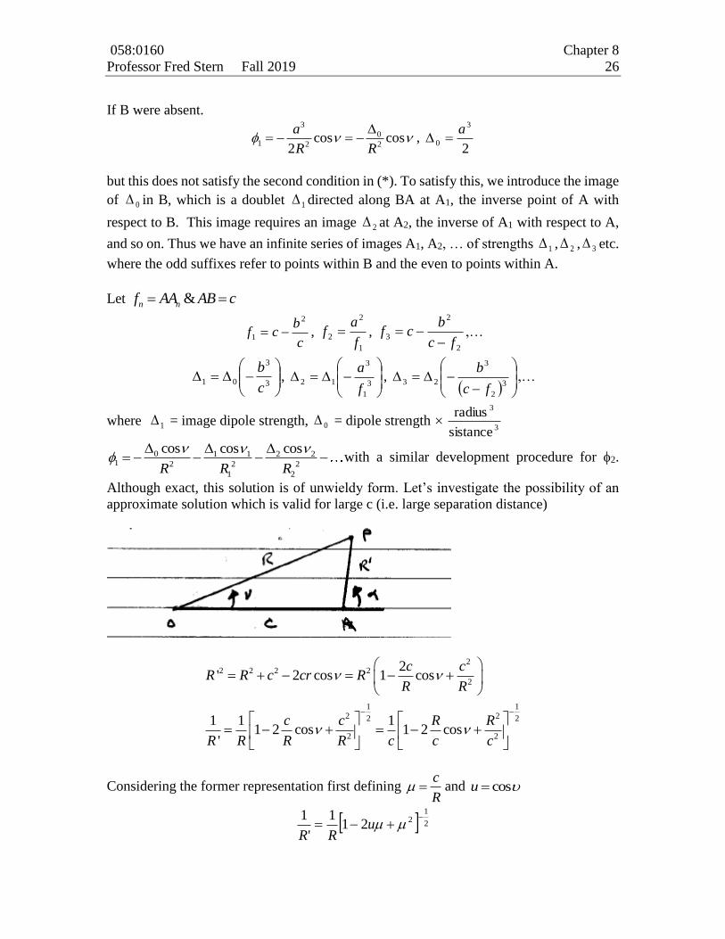
approximate solution which is valid for large c (i.e. large separation distance)
22 2 2 2
2
1 12 22 2
2 2
2' 2 cos 1 cos
1 1 11 2 cos 1 2 cos
'
c cR R c cr R
R R
c c R R
R R R R c c c
Considering the former representation first defining c
R and cosu
2
1221
1
'
1 u
RR
058:0160 Chapter 8
Professor Fred Stern Fall 2019 27
By the binomial theorem valid for 1x
3
3
2
2102
1
1 xxxx , 10 and
n
nn
242
1231
Hence if 12 2 u
2
210
2
2
2
102
1
2 uPuPuPu
After collecting terms in powers of , where the Pn are Legendre functions of the first
kind (i.e. Legendre polynomials which are Legendre functions of the first kind of order
zero). Thus,
2
1 22 3
2
1 22 3
1 1: cos cos
'
1 1: cos cos
'
R RR C P P
R c c c
c cR C P P
R R R R
Next, consider a doublet of strength at A
3 12
2 2 2 22 2
coscos 1
'2 cos 2 cos
R c
R cR c cR R c cR
Thus,
2
1 2
2 2 3
2
1 2 32 3 4
2 cos 3 coscos 1:
'
1 2 3: cos cos cos
RP R PR c
R c c c
c cR c P P P
R R R
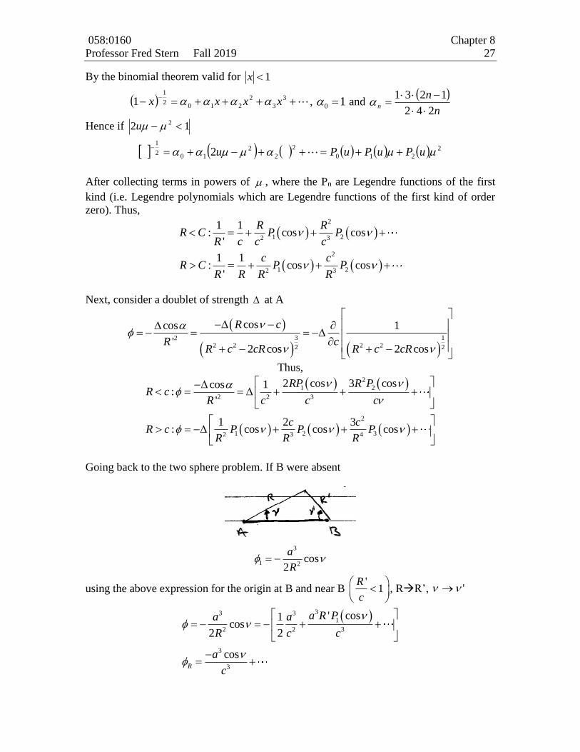
Going back to the two sphere problem. If B were absent
3
1 2cos
2
a
R
using the above expression for the origin at B and near B '
1R
c
, RR’, '
33 31
2 2 3
3
3
' cos1cos
2 2
cosR
a R Pa a
R c c
a
c
058:0160 Chapter 8
Professor Fred Stern Fall 2019 28
which can be cancelled by adding a term to the first approximation, i.e. 3 3 3
1 2 3 2
1 cos 1 cos '
2 2 '
a a b
R c R
to confirm this 3 3 3
1 2 3 3
1 3 'cos ' 1 cos
2 2
a a R a b
c c c R
3
3 3 3 ''1
' 3 3 '
cos ' cos( ) 0
a a bR b hot
R c c R
Similarly, the solution for f2 is
2
3 ' 3 3
2 3 2'
1 cos 1 cos
2 2
b a b
c RR
These approximate solutions are converted to 3c .
To find the kinetic energy of the fluid, we have
1
2A B
n n
S S
K dS dS
2 2
11 1 12 1 2 22 2
1
2 2A B
n
S S
K A U A U U A U dS
111 1 A
A
A dSn
, 222 2 B
B
A dSn
, 1 112 2 1A B
A B
A dS dSn n
where 22 sindS R d
3
113
2aA ,
3 3
12 3
2 a bA
c
, 3
223
2bA ,
3 32 2
1 1 1 2 2 23
1 2 1' '
4 4
a bK M U U U M U
c
: using the approximate form of the potentials
where 2 2
1 1 2 2
1 1' , '
4 4M U M U : masses of liquid displaced by sphere.
8.5 Complex variable and conformal mapping
This method provides a very powerful method for solving 2-D flow problems. Although
the method can be extended for arbitrary geometries, other techniques are equally useful.
Thus, the greatest application is for getting simple flow geometries for which it provides
closed form analytic solution which provides basic solutions and can be used to validate
numerical methods.
058:0160 Chapter 8
Professor Fred Stern Fall 2019 29
Function of a complex variable
Conformal mapping relies entirely on complex mathematics. Therefore, a brief review is
undertaken at this point.
A complex number z is a sum of a real and imaginary part; z = real + i imaginary
The term i, refers to the complex number
so that;
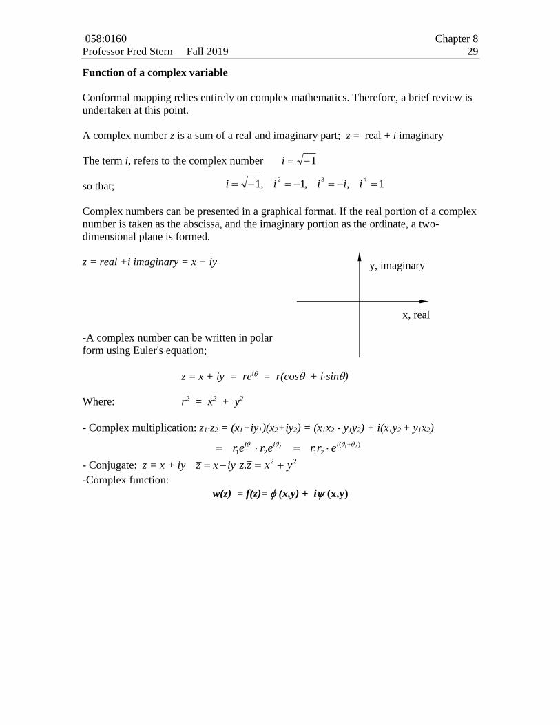
Complex numbers can be presented in a graphical format. If the real portion of a complex
number is taken as the abscissa, and the imaginary portion as the ordinate, a two-
dimensional plane is formed.
z = real +i imaginary = x + iy
-A complex number can be written in polar
form using Euler's equation;
z = x + iy = rei = r(cos + isin)
Where: r2 = x2 + y2
- Complex multiplication: z1z2 = (x1+iy1)(x2+iy2) = (x1x2 - y1y2) + i(x1y2 + y1x2)
- Conjugate: z = x + iy z x iy 22. yxzz
-Complex function:
w(z) = f(z)= (x,y) + i (x,y)
1i
1,,1,1432 iiiii
y, imaginary
x, real
)(
21212121
iii
errerer
058:0160 Chapter 8
Professor Fred Stern Fall 2019 30
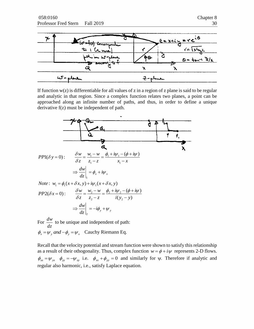
If function w(z) is differentiable for all values of z in a region of z plane is said to be regular
and analytic in that region. Since a complex function relates two planes, a point can be
approached along an infinite number of paths, and thus, in order to define a unique
derivative f(z) must be independent of path.
1 1 1
1 1
1
1 1 1
( )1( 0) :
: ( , ) ( , )
x x
w w i iwPP y
z z z x x
dwi
dz
Note w x x y i x x y
2 2 2
2 2
2
( )2( 0) :
( )
y y
w w i iwPP x
z z z i y y
dwi
dz
For dz
dw to be unique and independent of path:
x y y xand Cauchy Riemann Eq.
Recall that the velocity potential and stream function were shown to satisfy this relationship
as a result of their othogonality. Thus, complex function iw represents 2-D flows.
xx yx yy xy i.e. 0 yyxx and similarly for Therefore if analytic and
regular also harmonic, i.e., satisfy Laplace equation.
058:0160 Chapter 8
Professor Fred Stern Fall 2019 31
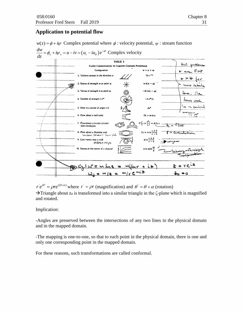
Application to potential flow
( )w z i Complex potential where : velocity potential, : stream function
i
x x r
dwi u iv u iu e
dz
Complex velocity
)('' ii reer where rr '(magnification) and ' (rotation)
Triangle about z0 is transformed into a similar triangle in the ζ-plane which is magnified
and rotated.
Implication:
-Angles are preserved between the intersections of any two lines in the physical domain
and in the mapped domain.
-The mapping is one-to-one, so that to each point in the physical domain, there is one and
only one corresponding point in the mapped domain.
For these reasons, such transformations are called conformal.
058:0160 Chapter 8
Professor Fred Stern Fall 2019 32
Usually the flow-field solution in the ζ-plane is known:
),(),()( iW
Then
),(),()( yxiyxzfWzw or &
Conformal mapping
The real power of the use of complex variables for flow analysis is through the application
of conformal mapping: techniques whereby a complicated geometry in the physical z-
domain is mapped onto a simple geometry in the ζ-plane (circular cylinder) for which the
flow-field solution is known. The flow-field solution in the z-plane is obtained by relating
the ζ-plane solution to the z-plane through the conformal transformation ζ=f(z) (or inverse
mapping z=g(ζ)).
Before considering the application of the technique, we shall review some of the more
important properties and theorems associated with it.
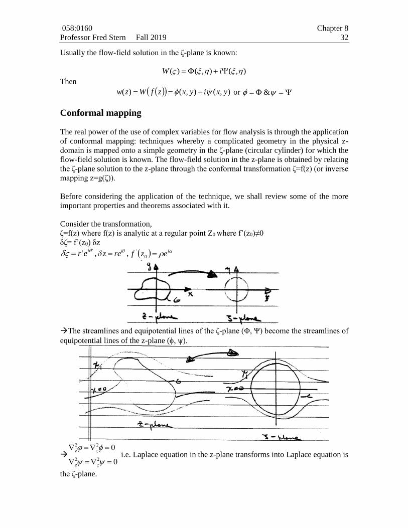
Consider the transformation,
ζ=f(z) where f(z) is analytic at a regular point Z0 where f’(z0)≠0
δζ= f’(z0) δz '' ier , iz re , iezf 0
'
The streamlines and equipotential lines of the ζ-plane (Φ, Ψ) become the streamlines of
equipotential lines of the z-plane (, ψ).
2 2
2 2
0
0
z
z
i.e. Laplace equation in the z-plane transforms into Laplace equation is
the ζ-plane.
058:0160 Chapter 8
Professor Fred Stern Fall 2019 33
The complex velocities in each plane are also simply related
'( )dw dw d dw
f zdz d dz d
( ) ( ) '( ) ( ( ))dw dW
z u iv U iV f z f zdz d
i.e. velocities in two planes are proportional.
Two independent theorems concerning conformal transformations are:
(1) Closed curves map to closed curves
(2) Rieman mapping theorem: an arbitrary closed profile can be mapped onto the unit
circle.
More theorems are given and discussed in AMF Section 43. Note that these are for the
interior problems, but are equally valid for the exterior problems through the inversion
mapping.
Many transformations have been investigated and are compiled in handbooks. The AMF
contains many examples:
1) Elementary transformations:
a) linear: 0 ,
bcad
dcz
bazw
b) corner flow: nAzw
c) Jowkowsky:
2cw
d) exponential: new
e) szw , s irational
2) Flow field for specific geometries
a) circle theorem
b) flat plate
c) circular arc
d) ellipse
e) Jowkowski foils
f) ogive (two circular areas)
g) Thin foil theory [solutions by mapping flat plate with thin foil BC onto unit
circle]
h) multiple bodies
3) Schwarz-Cristoffel mapping
4) Free-streamline theory
058:0160 Chapter 8
Professor Fred Stern Fall 2019 34
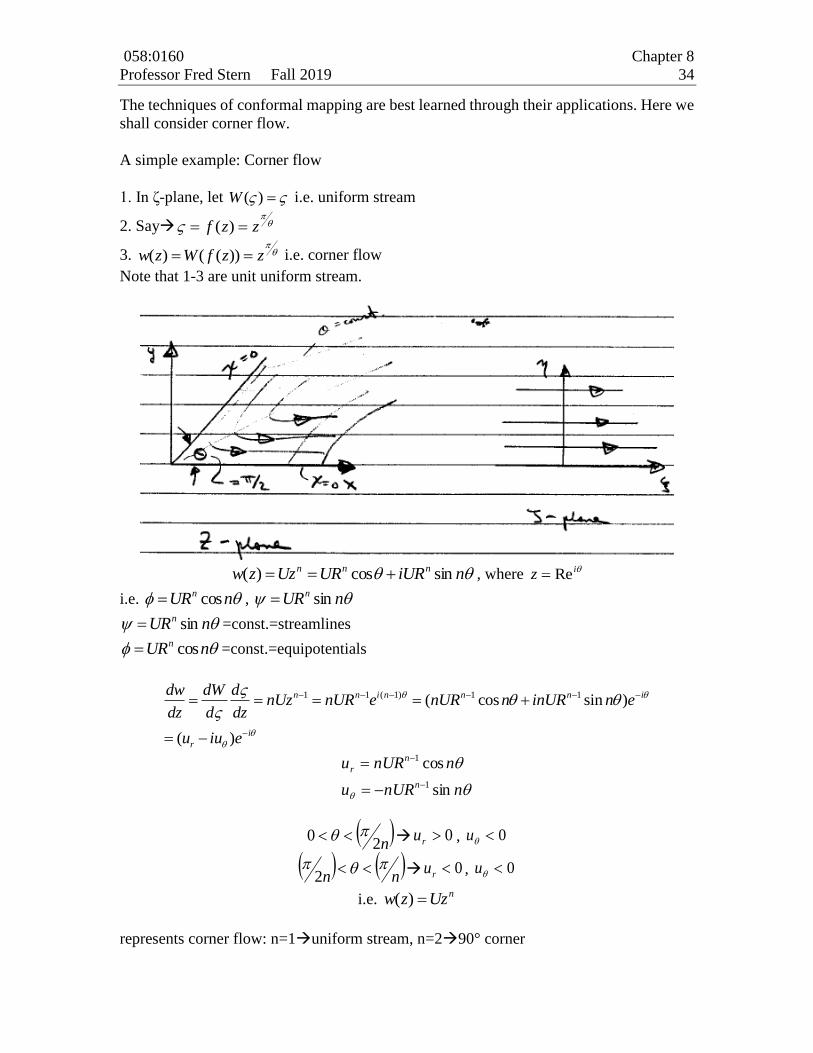
The techniques of conformal mapping are best learned through their applications. Here we
shall consider corner flow.
A simple example: Corner flow
1. In ζ-plane, let )(W i.e. uniform stream
2. Say
zzf )(
3.
zzfWzw ))(()( i.e. corner flow
Note that 1-3 are unit uniform stream.
niURURUzzw nnn sincos)( , where iz Re
i.e. nURn cos , nURn sin
nURn sin =const.=streamlines
nURn cos =const.=equipotentials
1 1 ( 1) 1 1( cos sin )
( )
n n i n n n i
i
r
dw dW dnUz nUR e nUR n inUR n e
dz d dz
u iu e
nnURu
nnURu
n
n
r
sin
cos
1
1
n2
0 0ru , 0u
nn
2
0ru , 0u
i.e. nUzzw )(
represents corner flow: n=1uniform stream, n=290° corner
058:0160 Chapter 8
Professor Fred Stern Fall 2019 35
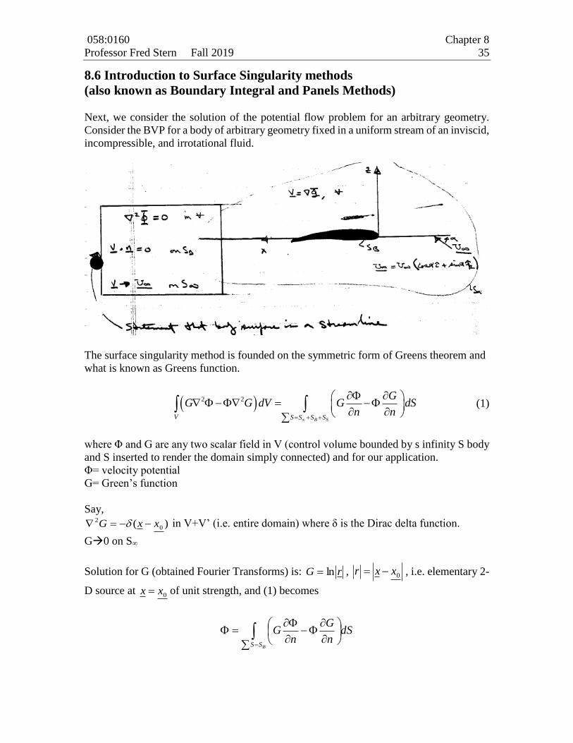
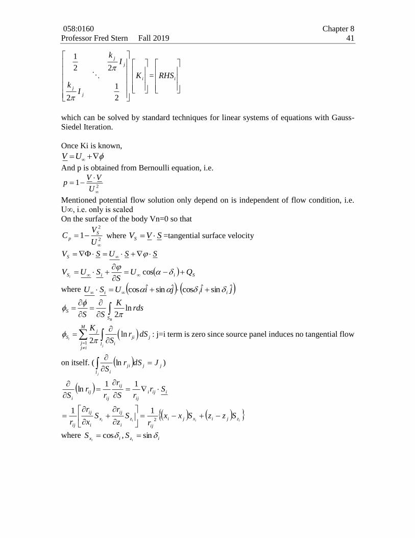
8.6 Introduction to Surface Singularity methods
(also known as Boundary Integral and Panels Methods)
Next, we consider the solution of the potential flow problem for an arbitrary geometry.
Consider the BVP for a body of arbitrary geometry fixed in a uniform stream of an inviscid,
incompressible, and irrotational fluid.
The surface singularity method is founded on the symmetric form of Greens theorem and
what is known as Greens function.
2 2
B SV S S S S
GG G dV G dS
n n
(1)
where Φ and G are any two scalar field in V (control volume bounded by s infinity S body
and S inserted to render the domain simply connected) and for our application.
Φ= velocity potential
G= Green’s function
Say,
)( 0
2 xxG in V+V’ (i.e. entire domain) where δ is the Dirac delta function.
G0 on S∞
Solution for G (obtained Fourier Transforms) is: rG ln , 0xxr , i.e. elementary 2-
D source at 0xx of unit strength, and (1) becomes
BSS
dSn
G
nG
058:0160 Chapter 8
Professor Fred Stern Fall 2019 36
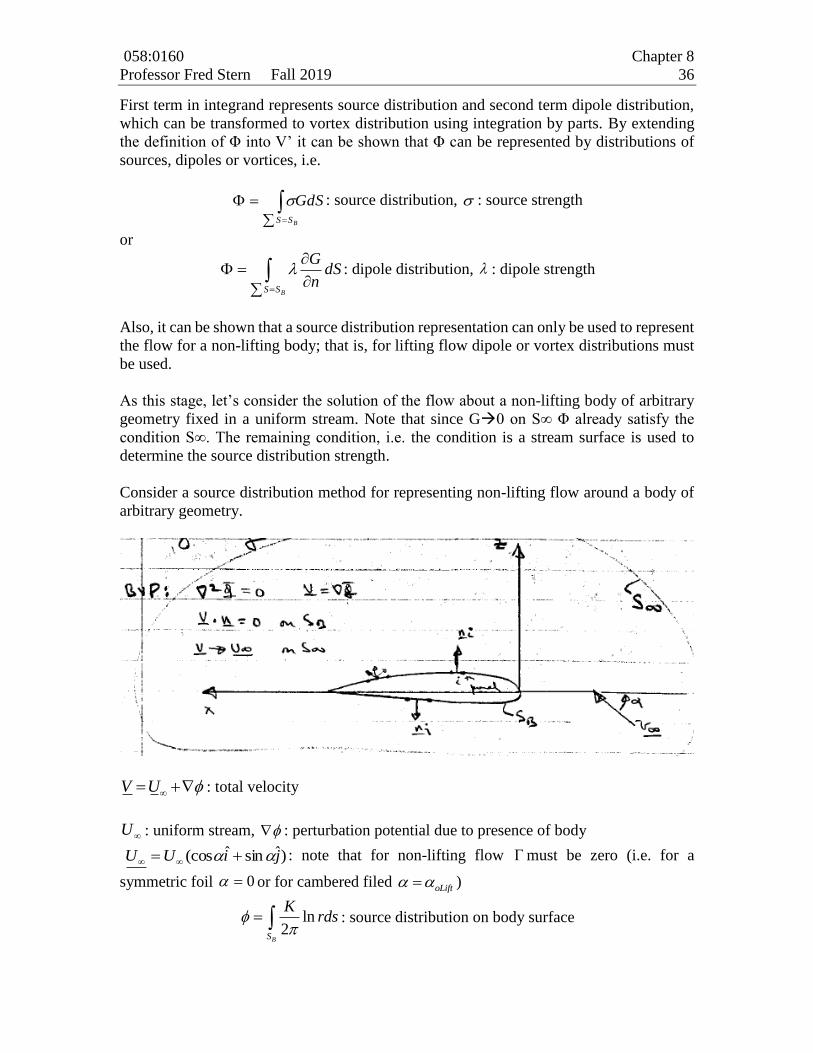
First term in integrand represents source distribution and second term dipole distribution,
which can be transformed to vortex distribution using integration by parts. By extending
the definition of Φ into V’ it can be shown that Φ can be represented by distributions of
sources, dipoles or vortices, i.e.
BSS
GdS : source distribution, : source strength
or
BSS
dSn
G : dipole distribution, : dipole strength
Also, it can be shown that a source distribution representation can only be used to represent
the flow for a non-lifting body; that is, for lifting flow dipole or vortex distributions must
be used.
As this stage, let’s consider the solution of the flow about a non-lifting body of arbitrary
geometry fixed in a uniform stream. Note that since G0 on S∞ Φ already satisfy the
condition S∞. The remaining condition, i.e. the condition is a stream surface is used to
determine the source distribution strength.
Consider a source distribution method for representing non-lifting flow around a body of
arbitrary geometry.
V U : total velocity
U : uniform stream, : perturbation potential due to presence of body
)ˆsinˆ(cos jiUU : note that for non-lifting flow must be zero (i.e. for a
symmetric foil 0 or for cambered filed oLift )
ln2
BS
Krds
: source distribution on body surface
058:0160 Chapter 8
Professor Fred Stern Fall 2019 37
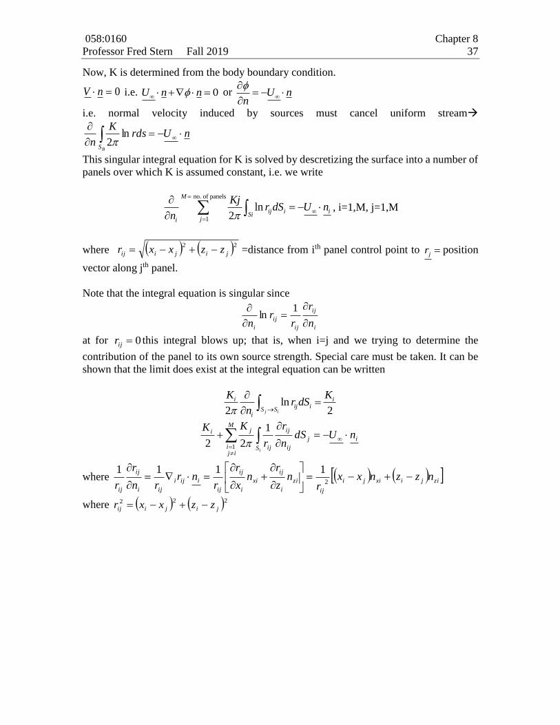
Now, K is determined from the body boundary condition.
0 nV i.e. 0U n n or U nn
i.e. normal velocity induced by sources must cancel uniform stream
nUrdsK
nBS
ln
2
This singular integral equation for K is solved by descretizing the surface into a number of
panels over which K is assumed constant, i.e. we write
no. of panels
1
ln2
M
ij i iSi
ji
Kjr dS U n
n
, i=1,M, j=1,M
where 22
jijiij zzxxr =distance from ith panel control point to jr position
vector along jth panel.
Note that the integral equation is singular since
i
ij
ij
ij
i n
r
rr
n
1ln
at for 0ijr this integral blows up; that is, when i=j and we trying to determine the
contribution of the panel to its own source strength. Special care must be taken. It can be
shown that the limit does exist at the integral equation can be written
ln2 2j i
i iij i
S Si
K Kr dS
n
M
iji S
ij
ij
ij
ij
ji
i
nUdSn
r
r
KK
1
1
22
where zijixiji
ij
zi
i
ij
xi
i
ij
ij
iiji
iji
ij
ij
nzznxxr
nz
rn
x
r
rnr
rn
r
r
2
1111
where 222
jijiij zzxxr
058:0160 Chapter 8
Professor Fred Stern Fall 2019 38
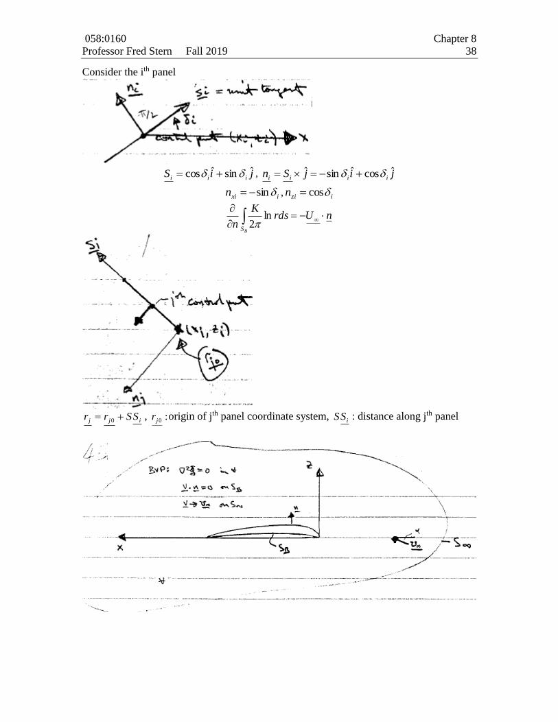
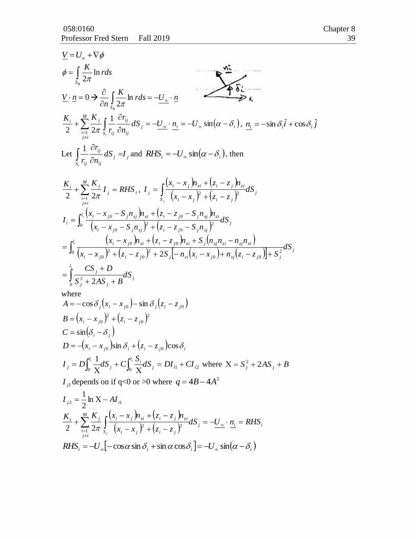
Consider the ith panel
jiS iiiˆsinˆcos , jijSn iiii
ˆcosˆsinˆ
ixin sin , izin cos
nUrdsK
nBS
ln
2
ijj SSrr 0, :0jr origin of jth panel coordinate system,
iSS : distance along jth panel
058:0160 Chapter 8
Professor Fred Stern Fall 2019 39
V U
ln2
BS
Krds
0 nV nUrdsK
nBS
ln
2
M
iji S
iij
ij
ij
ij
ji
i
UnUdSn
r
r
KK
1
sin1
22
, jin iii
ˆcosˆsin
Let j
S
j
ij
ij
ij
IdSn
r
ri
1and ii URHS sin , then
i
M
iji
j
ji RHSIKK
1 22
, j
S jiji
zijixiji
j dSzzxx
nzznxxI
j
22
j
l
jj
j
j
l
jjizjjizijjiji
xizjzixjjzijixiji
j
l
xjjjizjjji
zixjjjixizjjji
i
dSBASS
DCS
dSSzznxxnSzzxx
nnnnSnzznxx
dSnSzznSxx
nnSzznnSxxI
i
i
i
0
2
0 2
00
2
0
2
0
00
0 2
0
2
0
00
2
2
where
ijiiji
ji
jiji
jijjij
zzxxD
C
zzxxB
zzxxA
cossin
sin
sincos
00
2
0
2
0
00
2100
1iij
li
j
l
j CIDIdSS
CdSDIii
where BASS jj 22
1jI depends on if q<0 or >0 where 244 ABq
12 ln2
1ij AII
ii
M
iji
j
S jiji
zijixijiji RHSnUdSzzxx
nzznxxKK
j
1
2222
iiii UURHS sincossinsincos
058:0160 Chapter 8
Professor Fred Stern Fall 2019 40
i
M
iji
i
ji RHSIKK
1 22
: Matrix equation for Ki and can be solved using Standard
methods such as Gauss-Siedel Iteration.
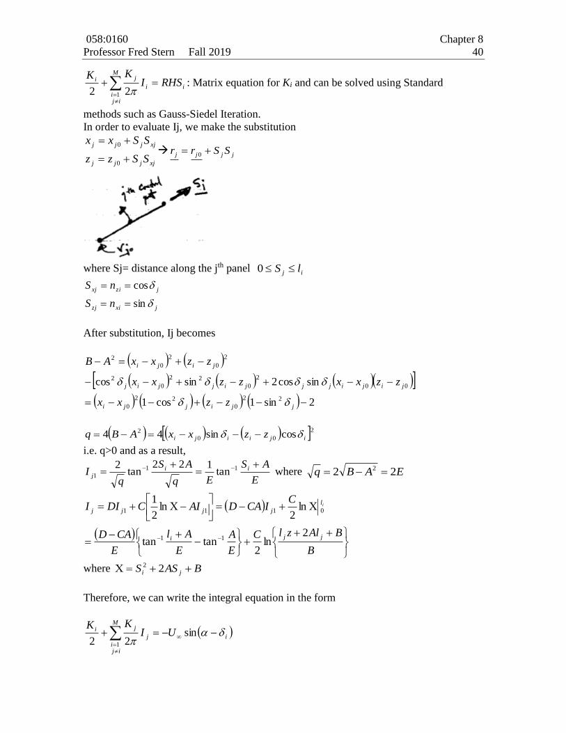
In order to evaluate Ij, we make the substitution
xjjjj
xjjjj
SSzz
SSxx
0
0
jjjj SSrr 0
where Sj= distance along the jth panel
ij lS 0
jxizj
jzixj
nS
nS
sin
cos
After substitution, Ij becomes
2sin1cos1
sincos2sincos
22
0
22
0
00
2
0
22
0
2
2
0
2
0
2
jjijji
jijijjjijjij
jiji
zzxx
zzxxzzxx
zzxxAB
200
2 cossin44 ijiiji zzxxABq
i.e. q>0 and as a result,
E
AS
Eq
AS
qI ii
j
11
1 tan122
tan2
where EABq 22 2
B
BAlzlC
E
A
E
Al
E
CAD
CICADAICDII
jji
l
jjjji
2ln
2tantan
ln2
ln2
1
11
0111
where BASS ji 22
Therefore, we can write the integral equation in the form
i
M
iji
j
ji UIKK
sin22 1
058:0160 Chapter 8
Professor Fred Stern Fall 2019 41
2
1
2
22
1
j
j
j
j
Ik
Ik
iK =
iRHS
which can be solved by standard techniques for linear systems of equations with Gauss-
Siedel Iteration.
Once Ki is known,
V U
And p is obtained from Bernoulli equation, i.e.
21
U
VVp
Mentioned potential flow solution only depend on is independent of flow condition, i.e.
U∞, i.e. only is scaled
On the surface of the body Vn=0 so that
2
2
1
U
VC S
p where SVVS =tangential surface velocity
SSUSVS
SiiS QUS
SUVi
cos
where jijiUSU iiiˆsinˆcosˆsinˆcos
ln2
B
S
S
Krds
S S
1
ln2i
j
Mj
S ji j
j ilj i
Kr dS
S
: j=i term is zero since source panel induces no tangential flow
on itself. ( j
l
jji
i
JdSrS
j
ln )
iiii zjixji
ij
z
i
ij
x
i
ij
ij
iiji
ij
ij
ij
ij
i
SzzSxxr
Sz
rS
x
r
r
SrrS
r
rr
S
2
11
11ln
where ixiS cos , izi
S sin
058:0160 Chapter 8
Professor Fred Stern Fall 2019 42
2
1
U
VC i
i
S
p , j
jij
ii J
KUV
1 2
cos
j
l
zjjjixjjji
zizxjjjixixjjji
j
S jiji
zijixiji
j
l
ij
ij
ij
dSSSzzSSxx
SSSzzSSSxx
dSzzxx
nzznxxdS
S
r
rJ
i
ji
0 2
0
2
0
00
22
1
where ixi
S cos ,izi
S sin , BASSSSzzSSxx jjzjjjixjjji 222
0
2
0
i
i
jj
j
ijijzizjxixjjiiiiji
dSCASS
DCS
SSSSSzzxx
0
2
0 sinsincoscossincos
1121
00
ln2
1cos
sincos
jjjjji
ijiiji
AICDICIDIC
zzxxD
B
BAllC
E
A
E
Al
E
ACDCIACDJ
jjj
jj
2
ln2
tantanln2
2
11
1
jijijjijijijji
jjijiji
jjijiji
jjijiiji
iijjiiji
jijiijiiji
ijijiiji
ijiiji
zzxx
zz
xx
zz
xx
zzxx
zzxx
zzxxACD
sincoscossincoscossinsincossin
sincoscossin1sin
cossinsincos1cos
sincoscossinsinsin
coscoscossinsincos
coscossinsinsincos
cossincos
sincos
00
2
0
2
0
2
0
2
0
00
00
00
where ji
E
ACD
sin
058:0160 Chapter 8
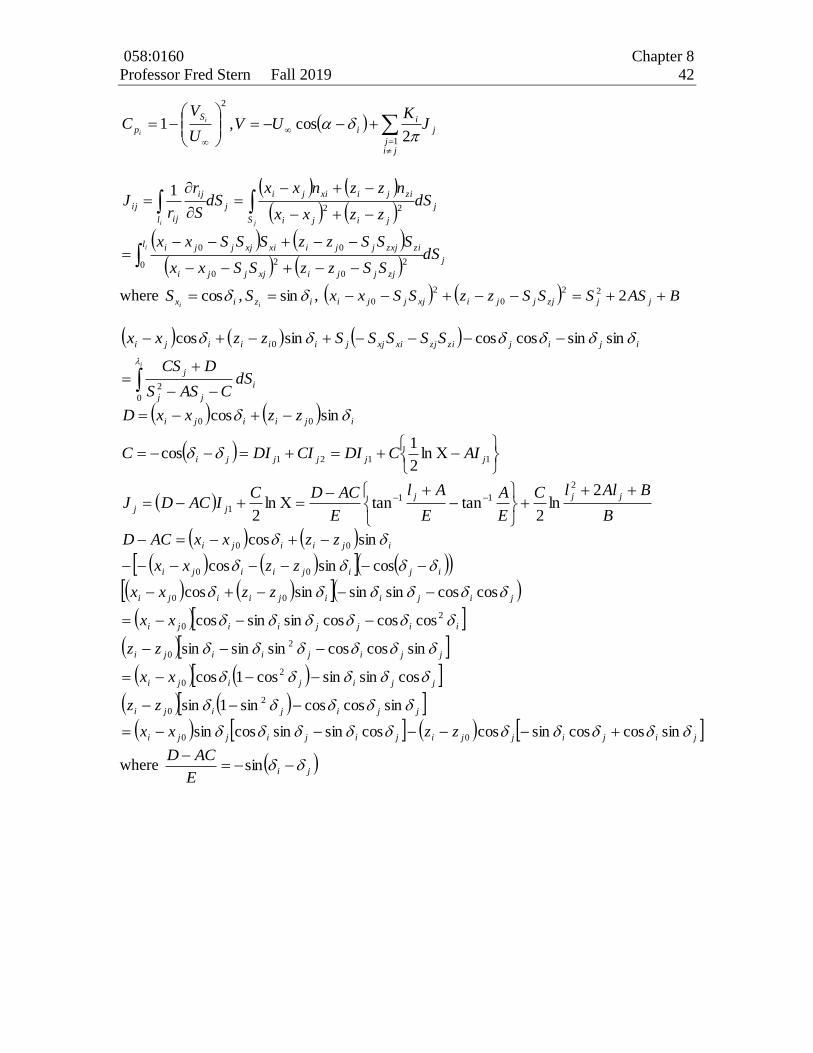
Professor Fred Stern Fall 2019 43
058:0160 Chapter 8
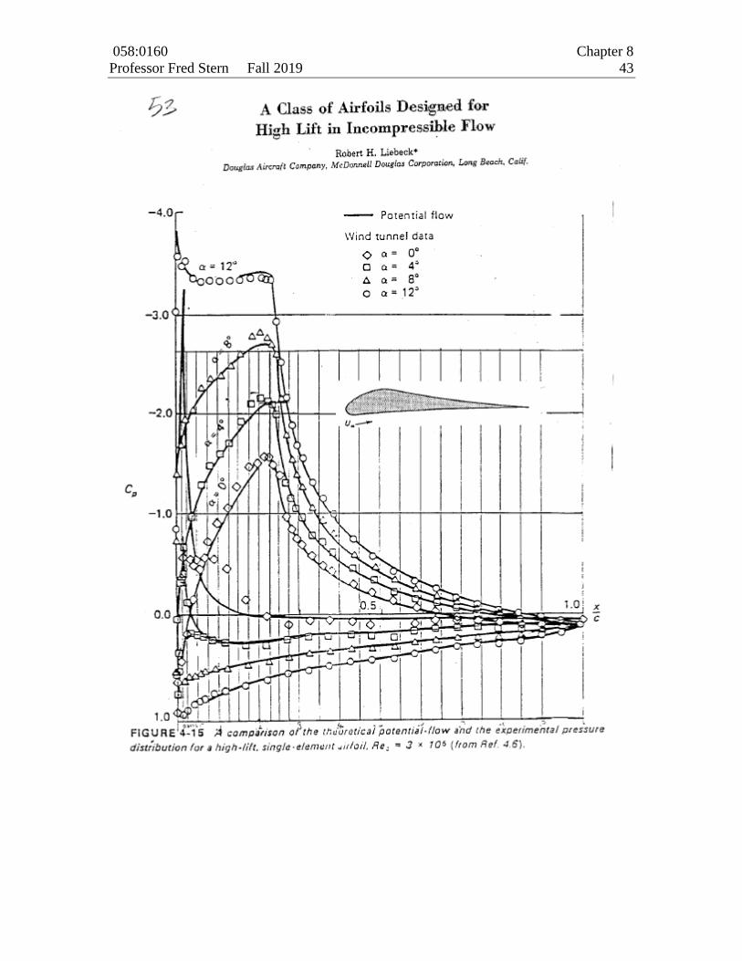
Professor Fred Stern Fall 2019 44
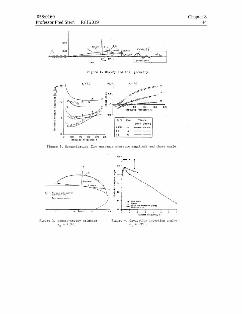
058:0160 Chapter 8
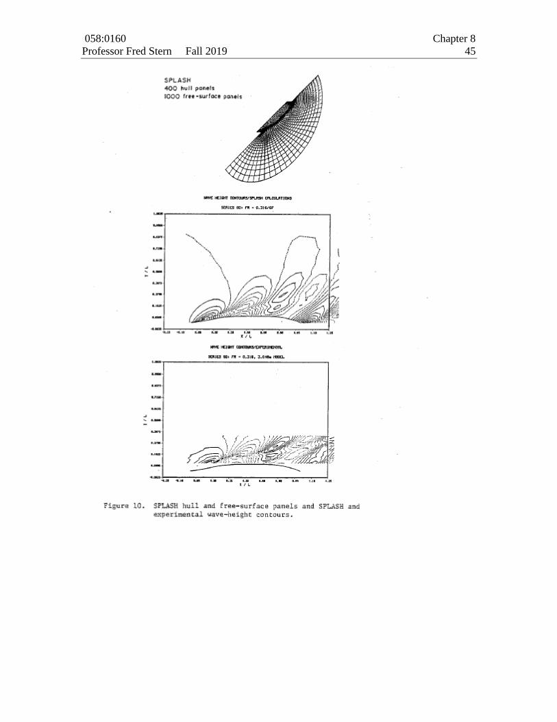
Professor Fred Stern Fall 2019 45
058:0160 Chapter 8
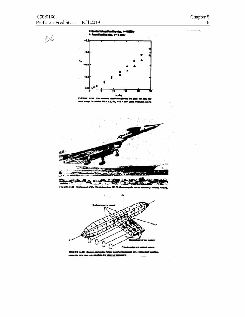
Professor Fred Stern Fall 2019 46
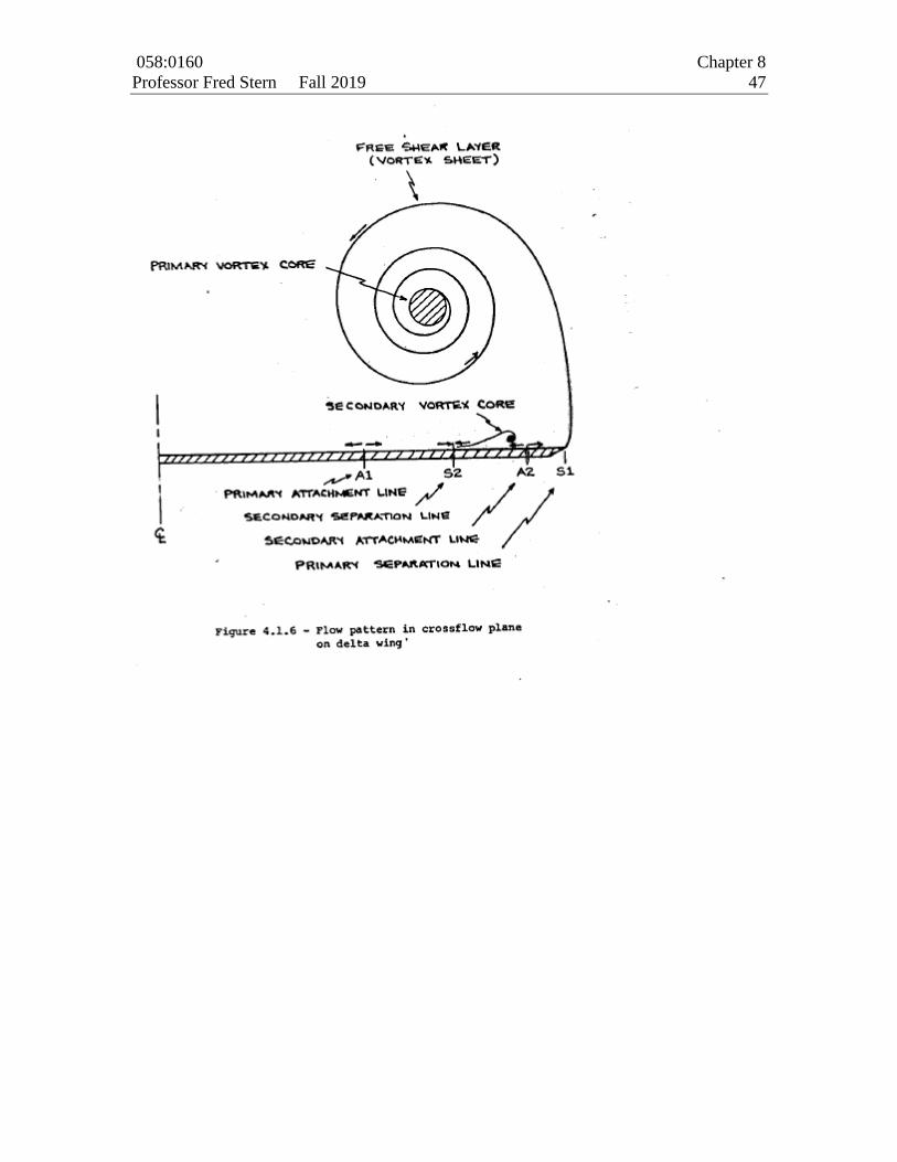
058:0160 Chapter 8
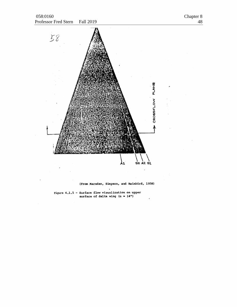
Professor Fred Stern Fall 2019 47
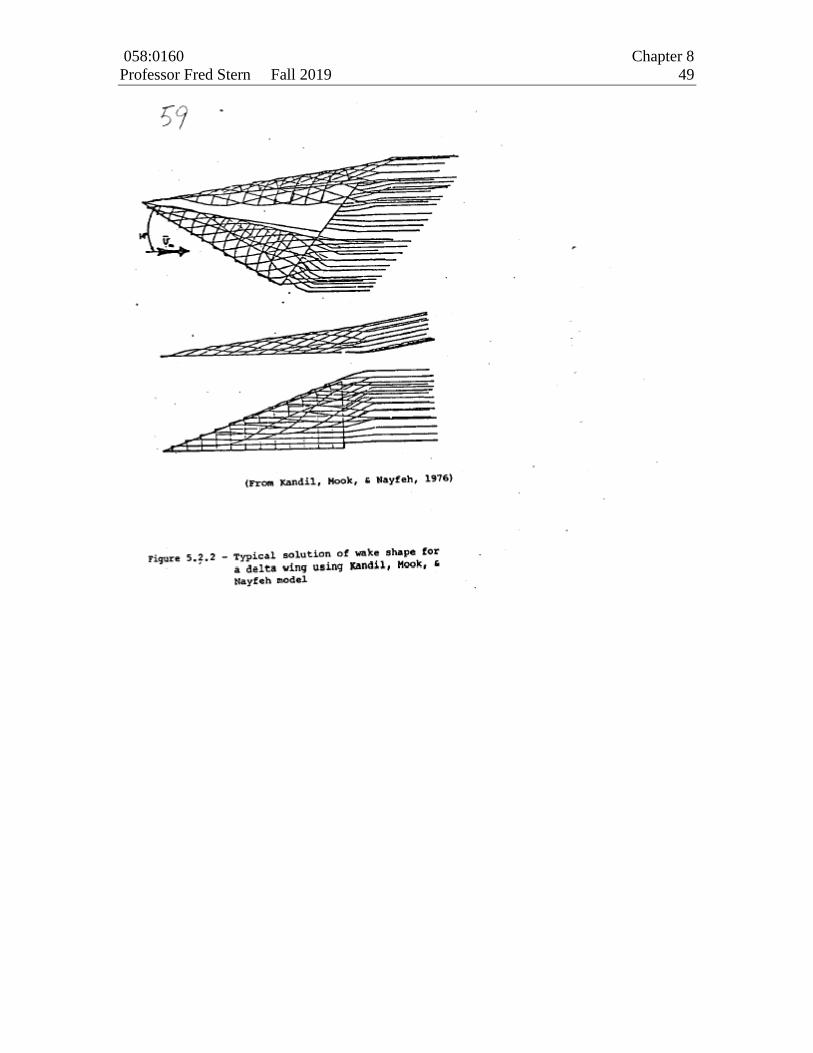
058:0160 Chapter 8
Professor Fred Stern Fall 2019 48
058:0160 Chapter 8
Professor Fred Stern Fall 2019 49
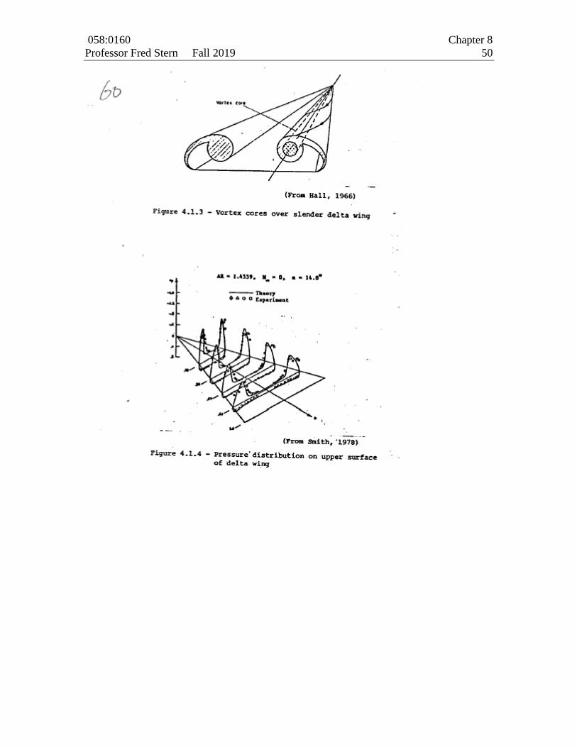
058:0160 Chapter 8
Professor Fred Stern Fall 2019 50
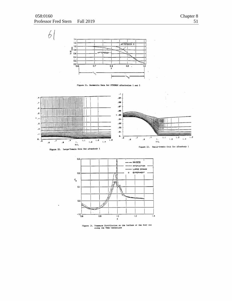
058:0160 Chapter 8
Professor Fred Stern Fall 2019 51