Embed Size (px)
Citation preview
8 DERIVATIONS INPREDICATE LOGIC
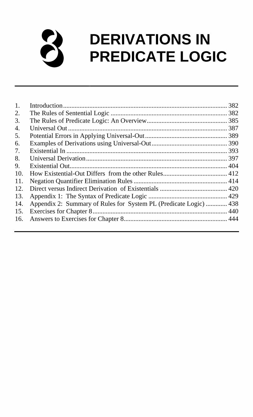
1. Introduction.................................................................................................... 3822. The Rules of Sentential Logic ....................................................................... 3823. The Rules of Predicate Logic: An Overview................................................. 3854. Universal Out ................................................................................................. 3875. Potential Errors in Applying Universal-Out .................................................. 3896. Examples of Derivations using Universal-Out .............................................. 3907. Existential In .................................................................................................. 3938. Universal Derivation...................................................................................... 3979. Existential Out................................................................................................ 40410. How Existential-Out Differs from the other Rules....................................... 41211. Negation Quantifier Elimination Rules ......................................................... 41412. Direct versus Indirect Derivation of Existentials ......................................... 42013. Appendix 1: The Syntax of Predicate Logic ................................................ 42914. Appendix 2: Summary of Rules for System PL (Predicate Logic) ............. 43815. Exercises for Chapter 8.................................................................................. 44016. Answers to Exercises for Chapter 8............................................................... 444
AB|~¬∀∃↔→∨¸

382 Hardegree, Symbolic Logic
1. INTRODUCTION
Having discussed the grammar of predicate logic and its relation to English,we now turn to the problem of argument validity in predicate logic.
Recall that, in Chapter 5, we developed the technique of formal derivation inthe context of sentential logic – specifically System SL. This is a technique to de-duce conclusions from premises in sentential logic. In particular, if an argument isvalid in sentential logic, then we can (in principle) construct a derivation of its con-clusion from its premises in System SL, and if it is invalid, then we cannot constructsuch a derivation.
In the present chapter, we examine the corresponding deductive system forpredicate logic – what will be called System PL (short for ‘predicate logic’). Asyou might expect, since the syntax (grammar) of predicate logic is considerablymore complex than the syntax of sentential logic, the method of derivation inSystem PL is correspondingly more complex than System SL.
On the other hand, anyone who has already mastered sentential logic deriva-tions can also master predicate logic derivations. The transition primarily involves(1) getting used to the new symbols and (2) practicing doing the new derivations(just like in sentential logic!). The practical converse, unfortunately, is also true.Anyone who hasn't already mastered sentential logic derivations will have tremen-dous difficulty with predicate logic derivations. Of course, it's still not too late tofigure out sentential derivations!
2. THE RULES OF SENTENTIAL LOGIC
We begin by stating the first principle of predicate logic derivations. To wit,
Every rule of System SL (sentential logic) is also a ruleof System PL (predicate logic).
The converse is not true; as we shall see in later sections, there are several rulespeculiar to predicate logic, i.e., rules that do not arise in sentential logic.
Since predicate logic adopts all the derivation rules of sentential logic, it is agood idea to review the salient features of sentential logic derivations.
First of all, the derivation rules divide into two categories; on the one hand,there are inference rules, which are upward-oriented; on the other hand, there areshow rules, which are downward-oriented.
There are numerous inference rules, but they divide into four basic categories.
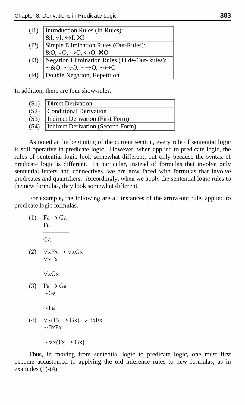
Chapter 8: Derivations in Predicate Logic 383
(I1) Introduction Rules (In-Rules):&I, ∨I, ↔I, ¸I
(I2) Simple Elimination Rules (Out-Rules):&O, ∨O, →O, ↔O, ¸O
(I3) Negation Elimination Rules (Tilde-Out-Rules):~&O, ~∨O, ~→O, ~↔O
(I4) Double Negation, Repetition
In addition, there are four show-rules.
(S1) Direct Derivation(S2) Conditional Derivation(S3) Indirect Derivation (First Form)(S4) Indirect Derivation (Second Form)
As noted at the beginning of the current section, every rule of sentential logicis still operative in predicate logic. However, when applied to predicate logic, therules of sentential logic look somewhat different, but only because the syntax ofpredicate logic is different. In particular, instead of formulas that involve onlysentential letters and connectives, we are now faced with formulas that involvepredicates and quantifiers. Accordingly, when we apply the sentential logic rules tothe new formulas, they look somewhat different.
For example, the following are all instances of the arrow-out rule, applied topredicate logic formulas.
(1) Fa → GaFa––––––––Ga
(2) ∀xFx → ∀xGx∀xFx––––––––––––∀xGx
(3) Fa → Ga~Ga––––––––~Fa
(4) ∀x(Fx → Gx) → ∃xFx~∃xFx–––––––––––––––––––~∀x(Fx → Gx)
Thus, in moving from sentential logic to predicate logic, one must firstbecome accustomed to applying the old inference rules to new formulas, as inexamples (1)-(4).

384 Hardegree, Symbolic Logic
The same thing applies to the show rules of sentential logic, and their associ-ated derivation strategies, which remain operative in predicate logic. Just as before,to show a conditional formula, one uses conditional derivation; similarly, to show anegation, or disjunction, or atomic formula, one uses indirect derivation. The onlydifference is that one must learn to apply these strategies to predicate logicformulas.
For example, consider the following show lines.
(1) ¬: Fa → Ga
(2) ¬: ∀xFx → ∀xGx
(3) ¬: ~Fa
(4) ¬: ~∃x(Fx & Gx)
(5) ¬: Rab
(6) ¬: ∀xFx ∨ ∀xGx
Every one of these is a formula for which we already have a ready-made derivationstrategy. In each case, either the formula is atomic, or its main connective is a sen-tential logic connective.
The formulas in (1) and (2) are conditionals, so we use conditional derivation,as follows.
(1) ¬: Fa → Ga CD Fa As ¬: Ga ??
(2) ¬: ∀xFx → ∀xGx CD ∀xFx As ¬: ∀xGx ??
The formulas in (3) and (4) are negations, so we use indirect derivation of thefirst form, as follows.
(3) ¬: ~Fa ID Fa As ¬: ¸ ??
(4) ¬: ~∃x(Fx & Gx) ID ∃x(Fx & Gx) As ¬: ¸ ??
The formula in (5) is atomic, so we use indirect derivation, supposing that adirect derivation doesn't look promising.
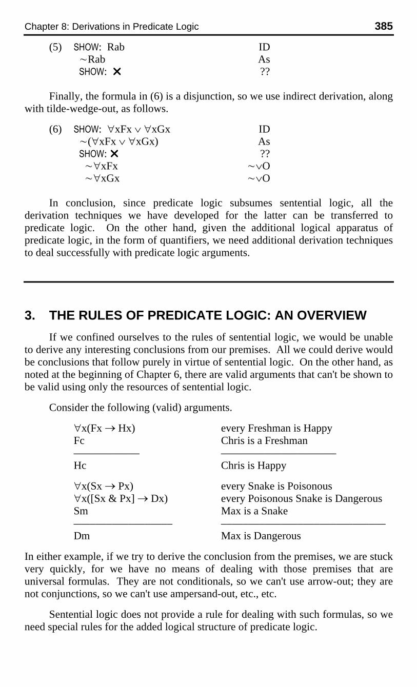
Chapter 8: Derivations in Predicate Logic 385
(5) ¬: Rab ID ~Rab As ¬: ¸ ??
Finally, the formula in (6) is a disjunction, so we use indirect derivation, alongwith tilde-wedge-out, as follows.
(6) ¬: ∀xFx ∨ ∀xGx ID ~(∀xFx ∨ ∀xGx) As ¬: ¸ ?? ~∀xFx ~∨O ~∀xGx ~∨O
In conclusion, since predicate logic subsumes sentential logic, all thederivation techniques we have developed for the latter can be transferred topredicate logic. On the other hand, given the additional logical apparatus ofpredicate logic, in the form of quantifiers, we need additional derivation techniquesto deal successfully with predicate logic arguments.
3. THE RULES OF PREDICATE LOGIC: AN OVERVIEW
If we confined ourselves to the rules of sentential logic, we would be unableto derive any interesting conclusions from our premises. All we could derive wouldbe conclusions that follow purely in virtue of sentential logic. On the other hand, asnoted at the beginning of Chapter 6, there are valid arguments that can't be shown tobe valid using only the resources of sentential logic.
Consider the following (valid) arguments.
∀x(Fx → Hx) every Freshman is HappyFc Chris is a Freshman–––––––––––– –––––––––––––––––––––Hc Chris is Happy
∀x(Sx → Px) every Snake is Poisonous∀x([Sx & Px] → Dx) every Poisonous Snake is DangerousSm Max is a Snake–––––––––––––––––– ––––––––––––––––––––––––––––––Dm Max is Dangerous
In either example, if we try to derive the conclusion from the premises, we are stuckvery quickly, for we have no means of dealing with those premises that areuniversal formulas. They are not conditionals, so we can't use arrow-out; they arenot conjunctions, so we can't use ampersand-out, etc., etc.
Sentential logic does not provide a rule for dealing with such formulas, so weneed special rules for the added logical structure of predicate logic.
386 Hardegree, Symbolic Logic
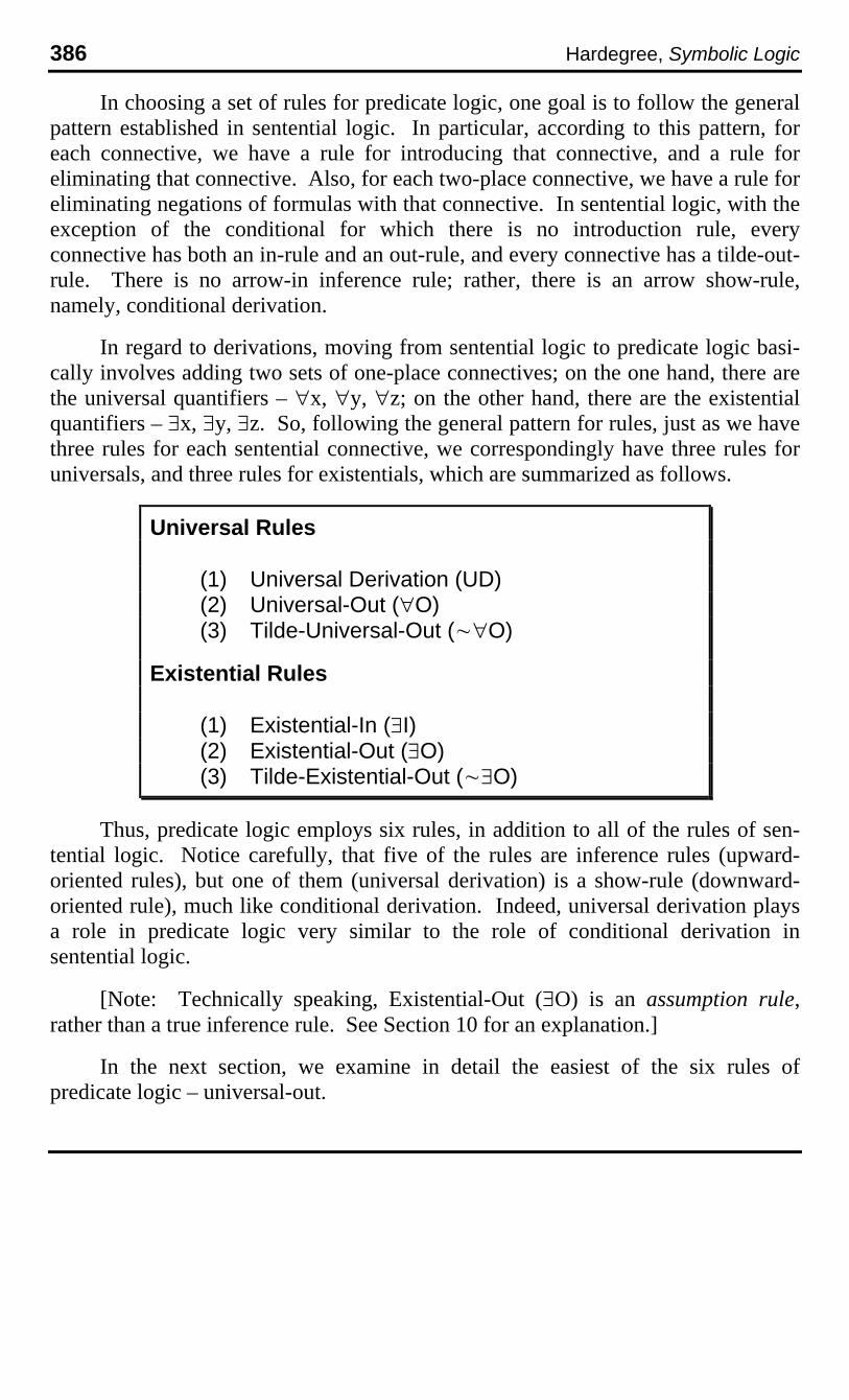
In choosing a set of rules for predicate logic, one goal is to follow the generalpattern established in sentential logic. In particular, according to this pattern, foreach connective, we have a rule for introducing that connective, and a rule foreliminating that connective. Also, for each two-place connective, we have a rule foreliminating negations of formulas with that connective. In sentential logic, with theexception of the conditional for which there is no introduction rule, everyconnective has both an in-rule and an out-rule, and every connective has a tilde-out-rule. There is no arrow-in inference rule; rather, there is an arrow show-rule,namely, conditional derivation.
In regard to derivations, moving from sentential logic to predicate logic basi-cally involves adding two sets of one-place connectives; on the one hand, there arethe universal quantifiers – ∀x, ∀y, ∀z; on the other hand, there are the existentialquantifiers – ∃x, ∃y, ∃z. So, following the general pattern for rules, just as we havethree rules for each sentential connective, we correspondingly have three rules foruniversals, and three rules for existentials, which are summarized as follows.
Universal Rules
(1) Universal Derivation (UD)(2) Universal-Out (∀O)(3) Tilde-Universal-Out (~∀O)
Existential Rules
(1) Existential-In (∃I)(2) Existential-Out (∃O)(3) Tilde-Existential-Out (~∃O)
Thus, predicate logic employs six rules, in addition to all of the rules of sen-tential logic. Notice carefully, that five of the rules are inference rules (upward-oriented rules), but one of them (universal derivation) is a show-rule (downward-oriented rule), much like conditional derivation. Indeed, universal derivation playsa role in predicate logic very similar to the role of conditional derivation insentential logic.
[Note: Technically speaking, Existential-Out (∃O) is an assumption rule,rather than a true inference rule. See Section 10 for an explanation.]
In the next section, we examine in detail the easiest of the six rules ofpredicate logic – universal-out.

Chapter 8: Derivations in Predicate Logic 387
4. UNIVERSAL OUT
The first, and easiest, rule we examine is universal-elimination (universal-out,for short). As its name suggests, it is a rule designed to decompose any formulawhose main connective is a universal quantifier (i.e., ∀x, ∀y, or ∀z).
The official statement of the rule goes as follows.
Universal-Out (∀O)
If one has an available line that is a universal formula,which is to say that it has the form ∀vF[v], where v isany variable, and F[v] is any formula in which v occursfree, then one is entitled to infer any substitution in-stance of F[v].
In symbols, this may be pictorially summarized as follows.
∀O: ∀vF[v]––––––F[n]
Here,
(1) v is any variable (x, y, z);
(2) n is any name (a-w);
(3) F[v] is any formula, and F[n] is the formula that results when n is substi-tuted for every occurrence of v that is free in F[v].
In order to understand this rule, it is best to look at a few examples.
Example 1: ∀xFx
This is by far the easiest example. In this v is x, and F[v] is Fx. To obtain a substi-tution instance of Fx one simply replaces x by a name, any name. Thus, all of thefollowing follow by ∀O:
Fa, Fb, Fc, Fd, etc.
Example 2: ∀yRyk
This is almost as easy. In this v is y, and F[v] is Ryk. To obtain a substitution in-stance of Ryk one simply replaces y by a name, any name. Thus, all of thefollowing follow by ∀O:
Rak, Rbk, Rck, Rdk, etc.
In both of these examples, the intuition behind the rule is quitestraightforward. In Example 1, the premise says that everything is an F; but if

388 Hardegree, Symbolic Logic
everything is an F, then any particular thing we care to mention is an F, so a is an F,b is an F, c is an F, etc. Similarly, in Example 2, the premise says that everythingbears relation R to k (for example, everyone respects Kay); but if everything bearsR to k, then any particular thing we care to mention bears R to k, so a bears R to k,b bears R to k, etc.
In examples 1 and 2, the formula F[v] is atomic. In the remaining examples,F[v] is molecular.
Example 3: ∀x(Fx → Gx)
In this v is x, and F[v] is Fx→Gx. To obtain a substitution instance, we replaceboth occurrences of x by a name, the same name for both occurrences. Thus, all ofthe following follow by ∀O.
Fa → Ga, Fb → Gb, Fc → Gc, etc.
In this example, the intuition underlying the rule may be less clear than in the firsttwo examples. The premise may be read in many ways in English, some morecolloquial than others.
(r1) every F is G(r2) everything is G if it's F(r3) everything is such that: if it is F, then it is G.
The last reading (r3) says that everything has a certain property, namely, that if it isF then it is G. But if everything has this property, then any particular thing we careto mention has the property. So a has the property, b has the property, etc. But tosay that a has the property is simply to say that if a is F then a is G; to say that b hasthe property is to say that if b is F then b is G. Both of these are applications ofuniversal-out.
Example 4: ∀x∃yRxy
Here, v is x, and F[v] is ∃yRxy. To obtain a substitution instance of ∃yRxy, onereplaces the one and only occurrence of x by a name, any name. Thus, thefollowing all follow by ∀O.
∃yRay, ∃yRby, ∃yRcy, ∃yRdy, etc.
The premise says that everything bears relation R to something or other. For exam-ple, it translates the English sentence ‘everyone respects someone (or other)’. But ifeveryone respects someone (or other), then anyone you care to mention respectssomeone, so a respects someone, b respects someone, etc.
Example 5: ∀x(Fx → ∀xGx)
Here, v is x, and F[v] is Fx→∀xGx. To obtain a substitution instance, one replacesevery free occurrence of x in Fx→∀xGx by a name. In this example, the firstoccurrence is free, but the remaining two are not, so we only replace the firstoccurrence. Thus, the following all follow by ∀O.
Fa → ∀xGx, Fb → ∀xGx, Fc → ∀xGx, etc.

Chapter 8: Derivations in Predicate Logic 389
This example is complicated by the presence of a second quantifier governing thesame variable, so we have to be especially careful in applying ∀O. Nevertheless,one's intuitions are not violated. The premise says that if anyone is an F then every-one is a G (recall the distinction between ‘if any’ and ‘if every’). From this it fol-lows that if a is an F then everyone is a G, and if b is an F then everyone is a G, etc.But that is precisely what we get when we apply ∀O to the premise.
5. POTENTIAL ERRORS IN APPLYING UNIVERSAL-OUT
There are basically two ways in which one can misapply the rule universal-out: (1) improper substitution; (2) improper application.
In the case of improper substitution, the rule is applied to an appropriate for-mula, namely, a universal, but an error is made in performing the substitution.Refer to the Appendix concerning correct and incorrect substitution instances. Thefollowing are a few examples of improper substitution.
(1) ∀xRxx ; to infer Rax, Rab, Rba WRONG!!!
(2) ∀x(Fx → Gx); to infer Fa → Gb, Fb → Gc WRONG!!!
(3) ∀x(Fx → ∀xGx); to infer Fa → ∀aGa, Fa → ∀xGa WRONG!!!
In the case of improper application, one attempts to apply the rule to a line thatdoes not have the appropriate form. Universal-out, as its name is intended to sug-gest, applies to universal formulas, not to atomic formulas, or existentials, or nega-tions, or conditionals, or biconditional, or conjunctions, or disjunctions.
Recall, in this connection, a very important principle.
INFERENCE RULES APPLYEXCLUSIVELY TO WHOLE LINES,
NOT TO PIECES OF LINES.
The following are examples of improper application of universal-out.
(4) ∀xFx → ∀xGx
to infer Fa → ∀xGx WRONG!!!to infer ∀xFx → Ga WRONG!!!to infer Fa → Gb WRONG!!!
In each case, the error is the same – specifically, applying universal-out to aformula that does not have the appropriate form. Now, the formula in question isnot a universal, but is rather a conditional; so the appropriate elimination rule is notuniversal-out, but rather arrow-out (which, of course, requires an additional prem-ise).
390 Hardegree, Symbolic Logic
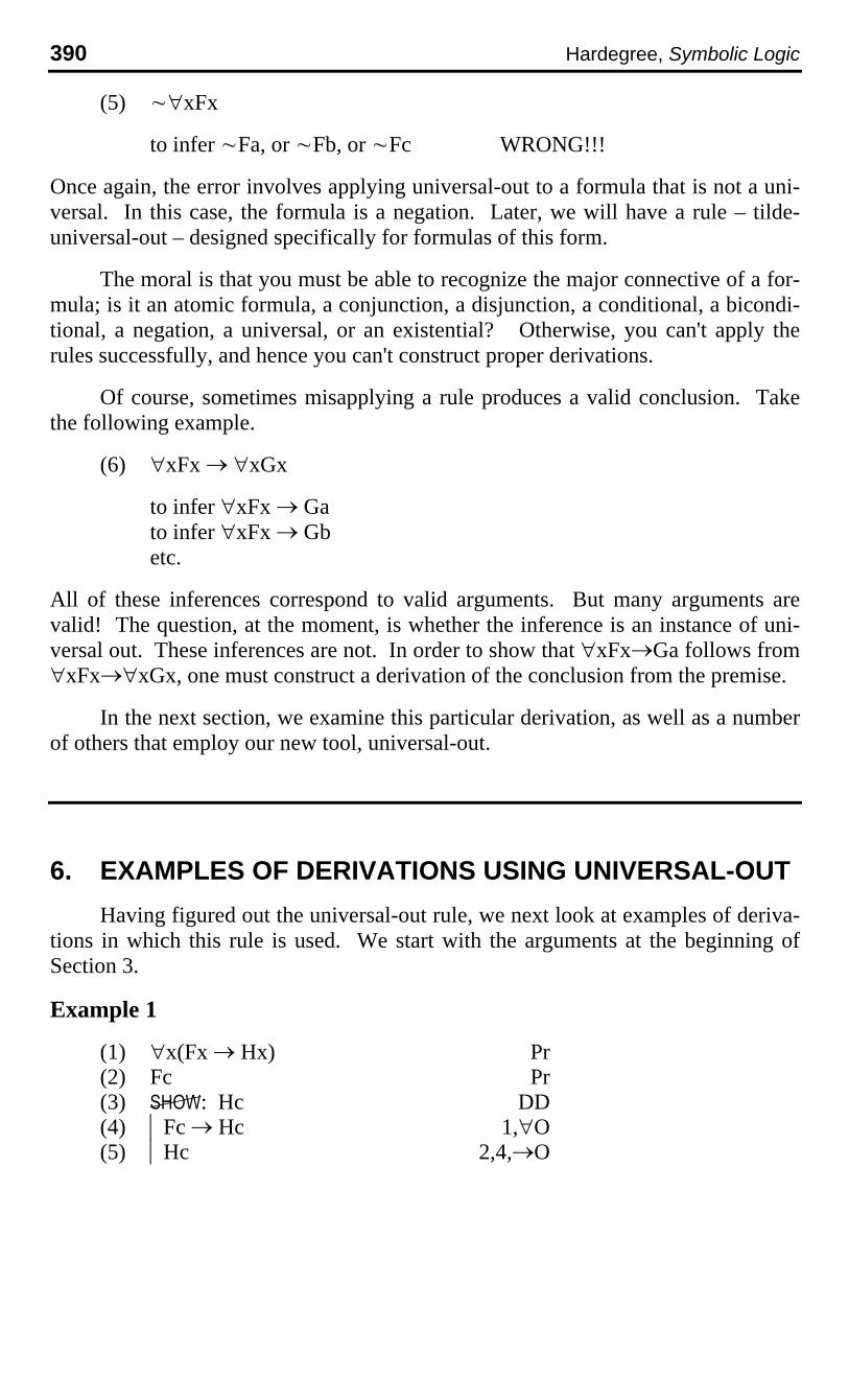
(5) ~∀xFx
to infer ~Fa, or ~Fb, or ~Fc WRONG!!!
Once again, the error involves applying universal-out to a formula that is not a uni-versal. In this case, the formula is a negation. Later, we will have a rule – tilde-universal-out – designed specifically for formulas of this form.
The moral is that you must be able to recognize the major connective of a for-mula; is it an atomic formula, a conjunction, a disjunction, a conditional, a bicondi-tional, a negation, a universal, or an existential? Otherwise, you can't apply therules successfully, and hence you can't construct proper derivations.
Of course, sometimes misapplying a rule produces a valid conclusion. Takethe following example.
(6) ∀xFx → ∀xGx
to infer ∀xFx → Gato infer ∀xFx → Gbetc.
All of these inferences correspond to valid arguments. But many arguments arevalid! The question, at the moment, is whether the inference is an instance of uni-versal out. These inferences are not. In order to show that ∀xFx→Ga follows from∀xFx→∀xGx, one must construct a derivation of the conclusion from the premise.
In the next section, we examine this particular derivation, as well as a numberof others that employ our new tool, universal-out.
6. EXAMPLES OF DERIVATIONS USING UNIVERSAL-OUT
Having figured out the universal-out rule, we next look at examples of deriva-tions in which this rule is used. We start with the arguments at the beginning ofSection 3.
Example 1
(1) ∀x(Fx → Hx) Pr(2) Fc Pr(3) : Hc DD(4) |Fc → Hc 1,∀O(5) |Hc 2,4,→O
Chapter 8: Derivations in Predicate Logic 391
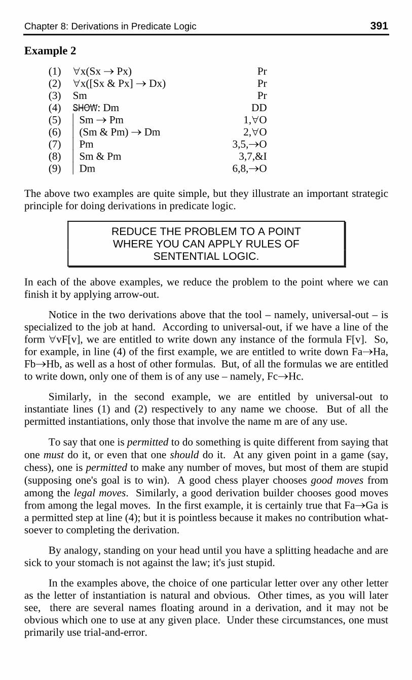
Example 2
(1) ∀x(Sx → Px) Pr(2) ∀x([Sx & Px] → Dx) Pr(3) Sm Pr(4) : Dm DD(5) |Sm → Pm 1,∀O(6) |(Sm & Pm) → Dm 2,∀O(7) |Pm 3,5,→O(8) |Sm & Pm 3,7,&I(9) |Dm 6,8,→O
The above two examples are quite simple, but they illustrate an important strategicprinciple for doing derivations in predicate logic.
REDUCE THE PROBLEM TO A POINTWHERE YOU CAN APPLY RULES OF
SENTENTIAL LOGIC.
In each of the above examples, we reduce the problem to the point where we canfinish it by applying arrow-out.
Notice in the two derivations above that the tool – namely, universal-out – isspecialized to the job at hand. According to universal-out, if we have a line of theform ∀vF[v], we are entitled to write down any instance of the formula F[v]. So,for example, in line (4) of the first example, we are entitled to write down Fa→Ha,Fb→Hb, as well as a host of other formulas. But, of all the formulas we are entitledto write down, only one of them is of any use – namely, Fc→Hc.
Similarly, in the second example, we are entitled by universal-out toinstantiate lines (1) and (2) respectively to any name we choose. But of all thepermitted instantiations, only those that involve the name m are of any use.
To say that one is permitted to do something is quite different from saying thatone must do it, or even that one should do it. At any given point in a game (say,chess), one is permitted to make any number of moves, but most of them are stupid(supposing one's goal is to win). A good chess player chooses good moves fromamong the legal moves. Similarly, a good derivation builder chooses good movesfrom among the legal moves. In the first example, it is certainly true that Fa→Ga isa permitted step at line (4); but it is pointless because it makes no contribution what-soever to completing the derivation.
By analogy, standing on your head until you have a splitting headache and aresick to your stomach is not against the law; it's just stupid.
In the examples above, the choice of one particular letter over any other letteras the letter of instantiation is natural and obvious. Other times, as you will latersee, there are several names floating around in a derivation, and it may not beobvious which one to use at any given place. Under these circumstances, one mustprimarily use trial-and-error.
392 Hardegree, Symbolic Logic
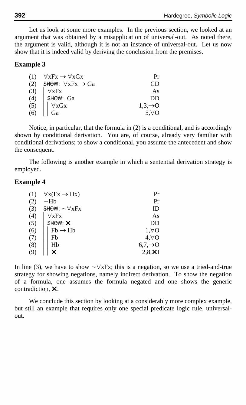
Let us look at some more examples. In the previous section, we looked at anargument that was obtained by a misapplication of universal-out. As noted there,the argument is valid, although it is not an instance of universal-out. Let us nowshow that it is indeed valid by deriving the conclusion from the premises.
Example 3
(1) ∀xFx → ∀xGx Pr(2) : ∀xFx → Ga CD(3) |∀xFx As(4) |: Ga DD(5) ||∀xGx 1,3,→O(6) ||Ga 5,∀O
Notice, in particular, that the formula in (2) is a conditional, and is accordinglyshown by conditional derivation. You are, of course, already very familiar withconditional derivations; to show a conditional, you assume the antecedent and showthe consequent.
The following is another example in which a sentential derivation strategy isemployed.
Example 4
(1) ∀x(Fx → Hx) Pr(2) ~Hb Pr(3) : ~∀xFx ID(4) |∀xFx As(5) |: ¸ DD(6) ||Fb → Hb 1,∀O(7) ||Fb 4,∀O(8) ||Hb 6,7,→O(9) ||¸ 2,8,¸I
In line (3), we have to show ~∀xFx; this is a negation, so we use a tried-and-truestrategy for showing negations, namely indirect derivation. To show the negationof a formula, one assumes the formula negated and one shows the genericcontradiction, ¸.
We conclude this section by looking at a considerably more complex example,but still an example that requires only one special predicate logic rule, universal-out.

Chapter 8: Derivations in Predicate Logic 393
Example 5
(1) ∀x(Fx → ∀yRxy) Pr(2) ∀x∀y(Rxy → ∀zGz) Pr(3) ~Gb Pr(4) : ~Fa ID(5) |Fa As(6) |: ¸ DD(7) ||Fa → ∀yRay 1,∀O(8) ||∀yRay 5,7,→O(9) ||Rab 8,∀O(10) ||∀y(Ray → ∀zGz) 2,∀O(11) ||Rab → ∀zGz 10,∀O(12) ||∀zGz 9,11,→O(13) ||Gb 12,∀O(14) ||¸ 3,13,¸I
If you can figure out this derivation, better yet if you can reproduce it yourself, thenyou have truly mastered the universal-out rule!
7. EXISTENTIAL IN
Of the six rules of predicate logic that we are eventually going to have, wehave now examined only one – universal-out. In the present section, we add onemore to the list.
The new rule, existential introduction (existential-in, ∃I) is officially stated asfollows.
Existential-In (∃I)
If formula F[n] is an available line, where F[n] is asubstitution instance of formula F[v], then one is entitledto infer the existential formula ∃vF[v].
In symbols, this may be pictorially summarized as follows.
∃I: F[n]––––––∃vF[v]
Here,
(1) v is any variable (x, y, z);
394 Hardegree, Symbolic Logic
(2) n is any name (a-w);
(3) F[v] is any formula, and F[n] is the formula that results when n is substi-tuted for every occurrence of v that is free in F[v].
Existential-In is very much like an upside-down version of Universal-Out.However, turning ∀O upside down to produce ∃I brings a small complication. In∀O, one begins with the formula F[v] with variable v, and one substitutes a name nfor the variable v. The only possible complication pertains to free and bound occur-rences of v. By contrast, in ∃I, one works backwards; one begins with the substitu-tion instance F[n] with name n, and one "de-substitutes" a variable v for n.Unfortunately, in many cases, de-substitution is radically different fromsubstitution. See examples below.
As with all rules of derivation, the best way to understand ∃I is to look at afew examples.
Example 1
have: Fb b is Finfer: ∃xFx; ∃yFy; ∃zFz at least one thing is F
Here, n is ‘b’, and F[n] is Fb, which is a substitution instance of three different for-mulas – Fx, Fy, and Fz. So the inferred formulas (which are alphabetic variants ofone another; see Appendix) can all be inferred in accordance with ∃I.
In Example 1, the intuition underlying the rule's application is quite straight-forward. The premise says that b is F. But if b is F, then at least one thing is F,which is what all three conclusions assert. One might understand this rule as sayingthat, if a particular thing has a property, then at least one thing has that property.
Example 2
have: Rjk j R's kinfer: ∃xRxk, ∃yRyk, ∃zRzk something R's kinfer: ∃xRjx, ∃yRjy, ∃zRjz j R's something
Here, we have two choices for n – ‘j’ and ‘k’. Treating ‘j’ as n, Rjk is a substitutioninstance of three different formulas – Rxk, Ryk, and Rzk, which are alphabeticvariants of one another. Treating ‘k’ as ‘n’, Rjk is a substitution instance of threedifferent formulas – Rjx, Rjy, and Rjz, which are alphabetic variants of one another.Thus, two different sets of formulas can be inferred in accordance with ∃I.
In Example 2, letting ‘R’ be ‘...respects...’ and ‘j’ be ‘Jay’ and ‘k’ be ‘Kay’,the premise says that Jay respects Kay. The conclusions are basically two(discounting alphabetic variants) – someone respects Kay, and Jay respects some-one.
Example 3
have: Fb & Hb
Here, n is ‘b’, and F[n] is Fb&Hb, which is a substitution instance of nine differentformulas:

Chapter 8: Derivations in Predicate Logic 395
(f1) Fx & Hx, Fy & Hy, Fz & Hz(f2) Fb & Hx, Fb & Hy, Fb & Hz(f3) Fx & Hb, Fy & Hb, Fz & Hb
So the following are all inferences that are in accord with ∃I:
infer:∃x(Fx & Hx), ∃y(Fy & Hy), ∃z(Fz & Hz)infer:∃x(Fb & Hx), ∃y(Fb & Hy), ∃z(Fb & Hz)infer:∃x(Fx & Hb), ∃y(Fy & Hb), ∃z(Fz & Hb)
In Example 3, three groups of formulas can be inferred by ∃I. In the case ofthe first group, the underlying intuition is fairly clear. The premise says that b is Fand b is H (i.e., b is both F and H), and the conclusions variously say that at leastone thing is both F and H. In the case of the remaining two groups, the intuition isless clear. These are permitted inferences, but they are seldom, if ever, used inactual derivations, so we will not dwell on them here.
In Example 3, there are two groups of conclusions that are somehow extrane-ous, although they are certainly permitted. The following example is quite similar,insofar as it involves two occurrences of the same name. However, the difference isthat the two extra groups of valid conclusions are not only legitimate but alsouseful.
Example 4
have: Rkk; k R's itself
infer:∃xRxx, ∃yRyy, ∃zRzz something R's itselfinfer:∃xRxk, ∃yRyk, ∃zRzk something R's kinfer:∃xRkx, ∃yRky, ∃zRkz k R's something
Here, n is ‘k’, and F[n] is Rkk, which is a substitution instance of nine differentformulas – Rxx, Rkx, Rxk, as well as the alphabetic variants involving ‘y’ and ‘z’.So the above inferences are all in accord with ∃I.
In Example 4, although the various inferences at first look a bit complicated,they are actually not too hard to understand. Letting ‘R’ be ‘...respects...’ and ‘k’ be‘Kay’, then the premise says that Kay respects Kay, or more colloquially Kay re-spects herself. But if Kay respects herself, then we can validly draw all of the fol-lowing conclusions.
(c1) someone respects her(him)self ∃xRxx(c2) someone respects Kay ∃xRxk(c3) Kay respects someone ∃xRkx
All of these follow from the premise ‘Kay respects herself’, and moreover they areall in accord with ∃I.
In all the previous examples, no premise involves a quantifier. The followingis the first such example, which introduces a further complication, as well.
396 Hardegree, Symbolic Logic
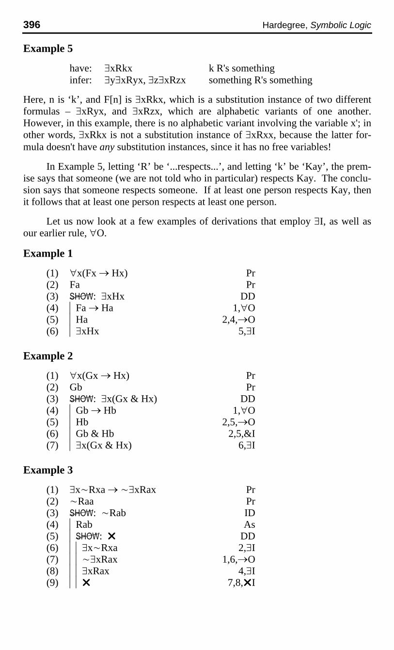
Example 5
have: ∃xRkx k R's somethinginfer: ∃y∃xRyx, ∃z∃xRzx something R's something
Here, n is ‘k’, and F[n] is ∃xRkx, which is a substitution instance of two differentformulas – ∃xRyx, and ∃xRzx, which are alphabetic variants of one another.However, in this example, there is no alphabetic variant involving the variable x'; inother words, ∃xRkx is not a substitution instance of ∃xRxx, because the latter for-mula doesn't have any substitution instances, since it has no free variables!
In Example 5, letting ‘R’ be ‘...respects...’, and letting ‘k’ be ‘Kay’, the prem-ise says that someone (we are not told who in particular) respects Kay. The conclu-sion says that someone respects someone. If at least one person respects Kay, thenit follows that at least one person respects at least one person.
Let us now look at a few examples of derivations that employ ∃I, as well asour earlier rule, ∀O.
Example 1
(1) ∀x(Fx → Hx) Pr(2) Fa Pr(3) : ∃xHx DD(4) |Fa → Ha 1,∀O(5) |Ha 2,4,→O(6) |∃xHx 5,∃I
Example 2
(1) ∀x(Gx → Hx) Pr(2) Gb Pr(3) : ∃x(Gx & Hx) DD(4) |Gb → Hb 1,∀O(5) |Hb 2,5,→O(6) |Gb & Hb 2,5,&I(7) |∃x(Gx & Hx) 6,∃I
Example 3
(1) ∃x~Rxa → ~∃xRax Pr(2) ~Raa Pr(3) : ~Rab ID(4) |Rab As(5) |: ¸ DD(6) ||∃x~Rxa 2,∃I(7) ||~∃xRax 1,6,→O(8) ||∃xRax 4,∃I(9) ||¸ 7,8,¸I

Chapter 8: Derivations in Predicate Logic 397
Example 4
(1) ∀x(∃yRxy → ∀yRxy) Pr(2) Raa Pr(3) : Rab DD(4) |∃yRay → ∀yRay 1,∀O(5) |∃yRay 2,∃I(6) |∀yRay 4,5,→O(7) |Rab 6,∀O
8. UNIVERSAL DERIVATION
We have now studied two rules, universal-out and existential-in. As statedearlier, every connective (other than tilde) has associated with it three rules, anintroduction rule, an elimination rule, and a negation-elimination rule. In thepresent section, we examine the introduction rule for the universal quantifier.
The first important point to observe is that, whereas the introduction rule forthe existential quantifier is an inference rule, the introduction rule for the universalquantifier is a show rule, called universal derivation (UD); compare this with condi-tional derivation. In other words, the rule is for dealing with lines of the form‘¬: ∀v...’.
Suppose one is faced with a derivation problem like the following.
(1) ∀x(Fx → Gx) Pr(2) ∀xFx Pr(3) ¬: ∀xGx ??
How do to go about completing the derivation? At the present, given its form, theonly derivation strategies available are direct derivation and indirect derivation(second form). However, in either approach, one quickly gets stuck. This is be-cause, as it stands, our derivation system is inadequate; we cannot derive ∀xFx'with the machinery currently at our disposal. So, we need a new rule.
Now what does the conclusion say? Well, ‘for any x, Gx’ says that everythingis G. This amounts to asserting every item in the following very long list.
(c1) Ga(c2) Gb(c3) Gc(c4) Gd
etc.
This is a very long list, one in which every particular thing in the universe is(eventually) mentioned. [Of course, we run out of ordinary names long before werun out of things to mention; so, in this situation, we have to suppose that we have atruly huge collection of names available.]
398 Hardegree, Symbolic Logic
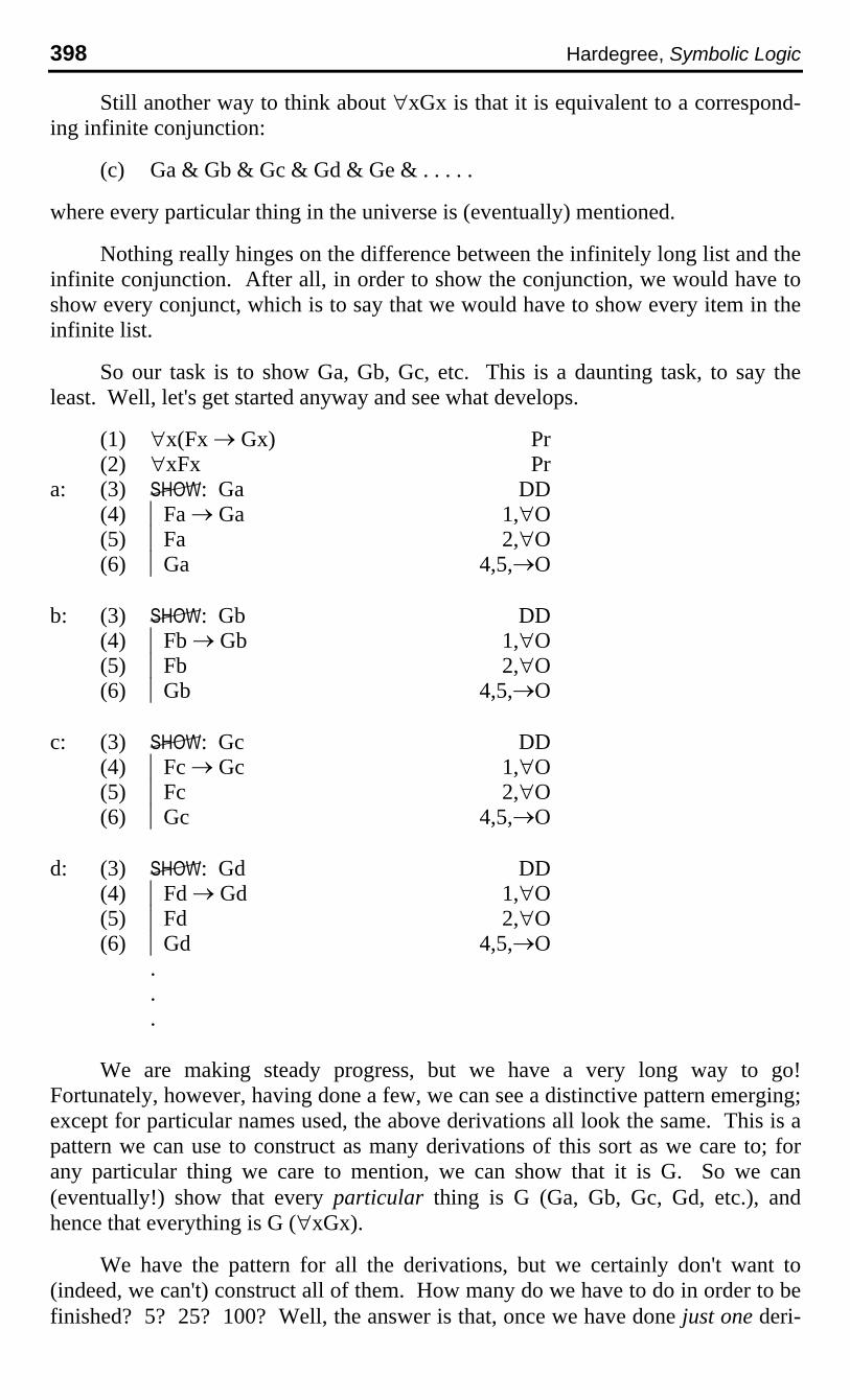
Still another way to think about ∀xGx is that it is equivalent to a correspond-ing infinite conjunction:
(c) Ga & Gb & Gc & Gd & Ge & . . . . .
where every particular thing in the universe is (eventually) mentioned.
Nothing really hinges on the difference between the infinitely long list and theinfinite conjunction. After all, in order to show the conjunction, we would have toshow every conjunct, which is to say that we would have to show every item in theinfinite list.
So our task is to show Ga, Gb, Gc, etc. This is a daunting task, to say theleast. Well, let's get started anyway and see what develops.
(1) ∀x(Fx → Gx) Pr(2) ∀xFx Pr
a: (3) : Ga DD(4) |Fa → Ga 1,∀O(5) |Fa 2,∀O(6) |Ga 4,5,→O
b: (3) : Gb DD(4) |Fb → Gb 1,∀O(5) |Fb 2,∀O(6) |Gb 4,5,→O
c: (3) : Gc DD(4) |Fc → Gc 1,∀O(5) |Fc 2,∀O(6) |Gc 4,5,→O
d: (3) : Gd DD(4) |Fd → Gd 1,∀O(5) |Fd 2,∀O(6) |Gd 4,5,→O
.
.
.
We are making steady progress, but we have a very long way to go!Fortunately, however, having done a few, we can see a distinctive pattern emerging;except for particular names used, the above derivations all look the same. This is apattern we can use to construct as many derivations of this sort as we care to; forany particular thing we care to mention, we can show that it is G. So we can(eventually!) show that every particular thing is G (Ga, Gb, Gc, Gd, etc.), andhence that everything is G (∀xGx).
We have the pattern for all the derivations, but we certainly don't want to(indeed, we can't) construct all of them. How many do we have to do in order to befinished? 5? 25? 100? Well, the answer is that, once we have done just one deri-
Chapter 8: Derivations in Predicate Logic 399
vation, we already have the pattern (model, mould) for every other derivation, so wecan stop after doing just one! The rest look the same, and are redundant, in effect.
This leads to the first (but not final) formulation of the principle of universalderivation.
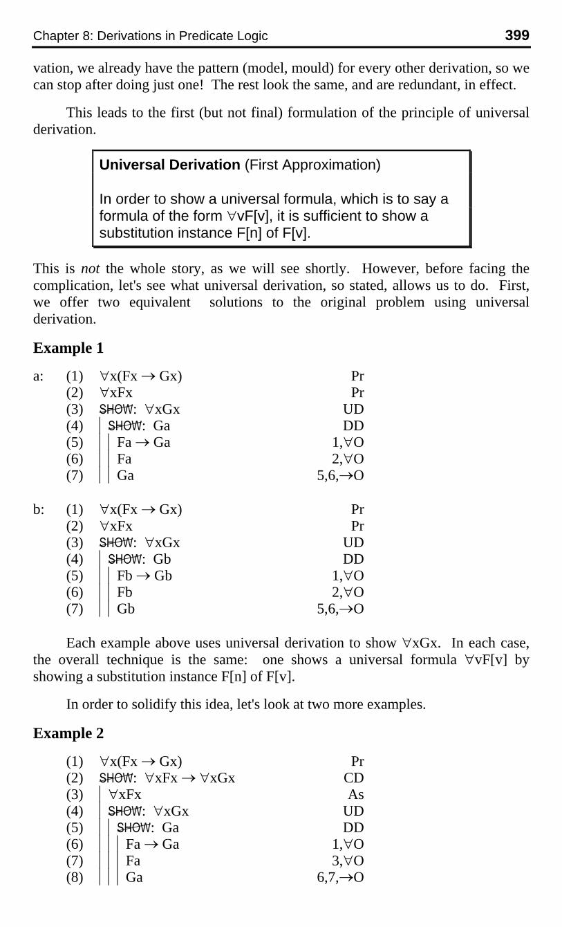
Universal Derivation (First Approximation)
In order to show a universal formula, which is to say aformula of the form ∀vF[v], it is sufficient to show asubstitution instance F[n] of F[v].
This is not the whole story, as we will see shortly. However, before facing thecomplication, let's see what universal derivation, so stated, allows us to do. First,we offer two equivalent solutions to the original problem using universalderivation.
Example 1
a: (1) ∀x(Fx → Gx) Pr(2) ∀xFx Pr(3) : ∀xGx UD(4) |: Ga DD(5) ||Fa → Ga 1,∀O(6) ||Fa 2,∀O(7) ||Ga 5,6,→O
b: (1) ∀x(Fx → Gx) Pr(2) ∀xFx Pr(3) : ∀xGx UD(4) |: Gb DD(5) ||Fb → Gb 1,∀O(6) ||Fb 2,∀O(7) ||Gb 5,6,→O
Each example above uses universal derivation to show ∀xGx. In each case,the overall technique is the same: one shows a universal formula ∀vF[v] byshowing a substitution instance F[n] of F[v].
In order to solidify this idea, let's look at two more examples.
Example 2
(1) ∀x(Fx → Gx) Pr(2) : ∀xFx → ∀xGx CD(3) |∀xFx As(4) |: ∀xGx UD(5) ||: Ga DD(6) |||Fa → Ga 1,∀O(7) |||Fa 3,∀O(8) |||Ga 6,7,→O

400 Hardegree, Symbolic Logic
In this example, line (2) asks us to show ∀xFx→∀xGx. One might be tempted touse universal derivation to show this, but this would be completely wrong. Why?Because ∀xFx→∀xGx is not a universal formula, but rather a conditional. Well,we already have a derivation technique for showing conditionals – conditionalderivation. That gives us the next two lines; we assume the antecedent, and weshow the consequent. So that gets us to line (4), which is to show ∀xGx'. Now,this formula is indeed a universal, so we use universal derivation; this means weimmediately write down a further show-line ‘¬: Ga’ (we could also write‘¬: Gb’, or ‘¬: Gc’, etc.). This is shown by direct derivation.
Example 3
(1) ∀x(Fx → Gx) Pr(2) ∀x(Gx → Hx) Pr(3) : ∀x(Fx → Hx) UD(4) |: Fa → Ha CD(5) ||Fa As(6) ||: Ha DD(7) |||Fa → Ga 1,∀O(8) |||Ga → Ha 2,∀O(9) |||Ga 5,7,→O(10) |||Ha 8,9,→O
In this example, we are asked to show ∀x(Fx→Gx), which is a universal formula,so we show it using universal derivation. This means that we immediately writedown a new show line, in this case ‘¬: Fa→Ha’; notice that Fa→Ha is asubstitution instance of Fx→Hx. Remember, to show ∀vF[v], one shows F[n],where F[n] is a substitution instance of F[v]. Now the problem is to show Fa→Ha;this is a conditional, so we use conditional derivation.
Having seen three successful uses of universal derivation, let us now examinean illegitimate use. Consider the following "proof" of a clearly invalid argument.
Example 4 (Invalid Argument!!)
(1) Fa & Ga Pr(2) ¬: ∀xGx UD(3) ¬: Ga DD WRONG!!!(4) Ga 1,&O
First of all, the fact that a is F and a is G does not logically imply that every-thing (or everyone) is G. From the fact that Adams is a Freshman who is Gloomy itdoes not follow that everyone is Gloomy. Then what went wrong with our tech-nique? We showed ∀xGx by showing an instance of Gx, namely Ga.
An important clue is forthcoming as soon as we try to generalize the aboveerroneous derivation to any other name. In the Examples 1-3, the fact that we use‘a’ is completely inconsequential; we could just as easily use any name, and thederivation goes through with equal success. But with the last example, we can in-deed show Ga, but that is all; we cannot show Gb or Gc or Gd. But in order to dem-
Chapter 8: Derivations in Predicate Logic 401
onstrate that everything is G, we have to show (in effect) that a is G, b is G, c is G,etc. In the last example, we have actually only shown that a is G.
In Examples 1-3, doing the derivation with ‘a’ was enough because this onederivation serves as a model for every other derivation. Not so in Example 4. Butwhat is the difference? When is a derivation a model derivation, and when is it nota model derivation?
Well, there is at least one conspicuous difference between the goodderivations and the bad derivation above. In every good derivation above, no nameappears in the derivation before the universal derivation, whereas in the badderivation above the name ‘a’ appears in the premises.
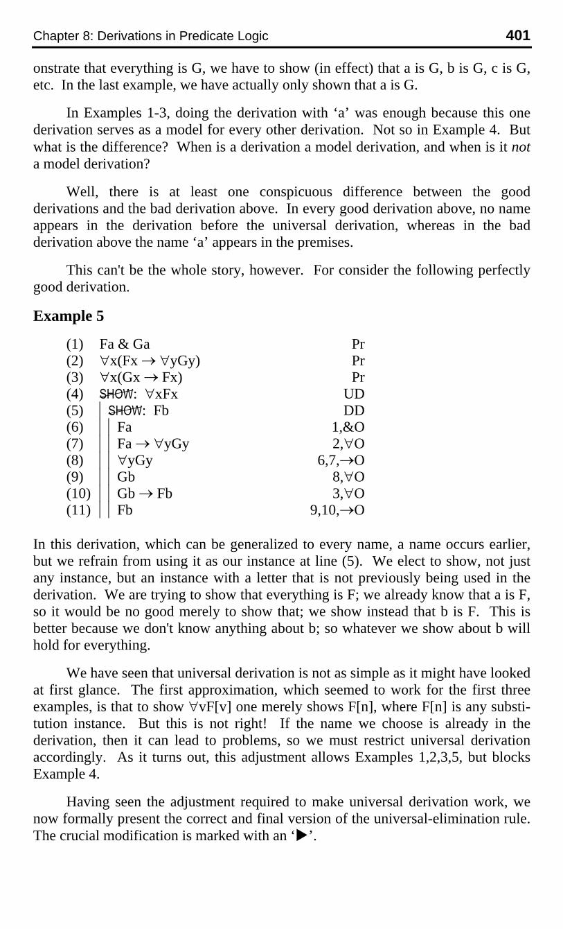
This can't be the whole story, however. For consider the following perfectlygood derivation.
Example 5
(1) Fa & Ga Pr(2) ∀x(Fx → ∀yGy) Pr(3) ∀x(Gx → Fx) Pr(4) : ∀xFx UD(5) |: Fb DD(6) ||Fa 1,&O(7) ||Fa → ∀yGy 2,∀O(8) ||∀yGy 6,7,→O(9) ||Gb 8,∀O(10) ||Gb → Fb 3,∀O(11) ||Fb 9,10,→O
In this derivation, which can be generalized to every name, a name occurs earlier,but we refrain from using it as our instance at line (5). We elect to show, not justany instance, but an instance with a letter that is not previously being used in thederivation. We are trying to show that everything is F; we already know that a is F,so it would be no good merely to show that; we show instead that b is F. This isbetter because we don't know anything about b; so whatever we show about b willhold for everything.
We have seen that universal derivation is not as simple as it might have lookedat first glance. The first approximation, which seemed to work for the first threeexamples, is that to show ∀vF[v] one merely shows F[n], where F[n] is any substi-tution instance. But this is not right! If the name we choose is already in thederivation, then it can lead to problems, so we must restrict universal derivationaccordingly. As it turns out, this adjustment allows Examples 1,2,3,5, but blocksExample 4.
Having seen the adjustment required to make universal derivation work, wenow formally present the correct and final version of the universal-elimination rule.The crucial modification is marked with an ‘u’.
402 Hardegree, Symbolic Logic
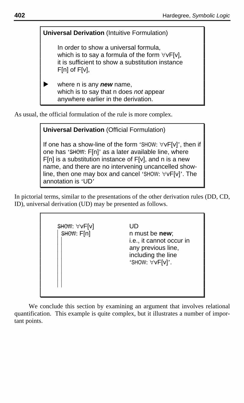
Universal Derivation (Intuitive Formulation)
In order to show a universal formula,which is to say a formula of the form ∀vF[v],it is sufficient to show a substitution instanceF[n] of F[v],
u where n is any new name,which is to say that n does not appearanywhere earlier in the derivation.
As usual, the official formulation of the rule is more complex.
Universal Derivation (Official Formulation)
If one has a show-line of the form ‘¬: ∀vF[v]’, then ifone has ‘: F[n]’ as a later available line, whereF[n] is a substitution instance of F[v], and n is a newname, and there are no intervening uncancelled show-line, then one may box and cancel ‘¬: ∀vF[v]’. Theannotation is ‘UD’
In pictorial terms, similar to the presentations of the other derivation rules (DD, CD,ID), universal derivation (UD) may be presented as follows.
: ∀vF[v] UD|: F[n] n must be new;|| i.e., it cannot occur in|| any previous line,|| including the line|| ‘¬: ∀vF[v]’.||||||
We conclude this section by examining an argument that involves relationalquantification. This example is quite complex, but it illustrates a number of impor-tant points.
Chapter 8: Derivations in Predicate Logic 403
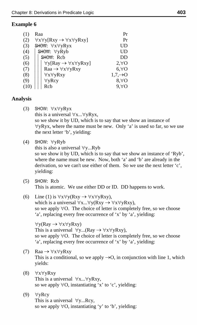
Example 6
(1) Raa Pr(2) ∀x∀y[Rxy → ∀x∀yRxy] Pr(3) : ∀x∀yRyx UD(4) |: ∀yRyb UD(5) ||: Rcb DD(6) |||∀y[Ray → ∀x∀yRxy] 2,∀O(7) |||Raa → ∀x∀yRxy 6,∀O(8) |||∀x∀yRxy 1,7,→O(9) |||∀yRcy 8,∀O(10) |||Rcb 9,∀O
Analysis
(3) ¬: ∀x∀yRyxthis is a universal ∀x...∀yRyx,so we show it by UD, which is to say that we show an instance of∀yRyx, where the name must be new. Only ‘a’ is used so far, so we usethe next letter ‘b’, yielding:
(4) ¬: ∀yRybthis is also a universal ∀y...Rybso we show it by UD, which is to say that we show an instance of ‘Ryb’,where the name must be new. Now, both ‘a’ and ‘b’ are already in thederivation, so we can't use either of them. So we use the next letter ‘c’,yielding:
(5) ¬: RcbThis is atomic. We use either DD or ID. DD happens to work.
(6) Line (1) is ∀x∀y(Rxy → ∀x∀yRxy),which is a universal ∀x...∀y(Rxy → ∀x∀yRxy),so we apply ∀O. The choice of letter is completely free, so we choose‘a’, replacing every free occurrence of ‘x’ by ‘a’, yielding:
∀y(Ray → ∀x∀yRxy)This is a universal ∀y...(Ray → ∀x∀yRxy),so we apply ∀O. The choice of letter is completely free, so we choose‘a’, replacing every free occurrence of ‘x’ by ‘a’, yielding:
(7) Raa → ∀x∀yRxyThis is a conditional, so we apply →O, in conjunction with line 1, whichyields:
(8) ∀x∀yRxyThis is a universal ∀x...∀yRxy,so we apply ∀O, instantiating ‘x’ to ‘c’, yielding:
(9) ∀yRcyThis is a universal ∀y...Rcy,so we apply ∀O, instantiating ‘y’ to ‘b’, yielding:
404 Hardegree, Symbolic Logic
(10) RcbThis is what we wanted to show!
By way of concluding this section, let us review the following points.
Having ∀vF[v] as an available line is very different fromhaving ‘¬: ∀vF[v]’ as a line.
In one case you have ∀vF[v];
in the other case, you don't have ∀vF[v];rather, you are trying to show it.
∀O applies when you have a universal;you can use any name whatsoever.
UD applies when you want a universal;you must use a new name.
9. EXISTENTIAL OUT
We now have three rules; we have both an elimination (out) and an introduc-tion (in) rule for ∀, and we have an introduction rule for ∃. At the moment, how-ever, we do not have an elimination rule for ∃. That is the topic of the current sec-tion.
Consider the following derivation problem.
(1) ∀x(Fx → Hx) Pr(2) ∃xFx Pr(3) ¬: ∃xHx ??
One possible English translation of this argument form goes as follows.
(1) every Freshman is happy(2) at least one person is a Freshman(3) therefore, at least one person is happy
This is indeed a valid argument. But how do we complete the correspondingderivation? The problem is the second premise, which is an existential formula. Atpresent, we do not have a rule specifically designed to decompose existentialformulas.
How should such a rule look? Well, the second premise is ∃xFx, which saysthat some thing (at least one thing) is F; however, it is not very specific; it doesn'tsay which particular thing is F. We know that at least one item in the following in-finite list is true, but we don't know which one it is.

Chapter 8: Derivations in Predicate Logic 405
(1) Fa(2) Fb(3) Fc(4) Fd
etc.
Equivalently, we know that the following infinite disjunction is true.
(d) Fa ∨ Fb ∨ Fc ∨ Fd ∨ ... ∨ ...
[Once again, we pretend that we have sufficiently many names to cover every singlething in the universe.]
The second premise ∃xFx says that at least one thing is F (some thing is F),but it provides no further information as to which thing in particular is F. Is it a? Isit b? We don't know given only the information conveyed by ∃xFx. So, what hap-pens if we simply assume that a is F. Adding this assumption yields the followingsubstitute problem.
(1) ∀x(Fx → Hx) Pr(2) ∃xFx Pr(3) ¬: ∃xHx DD(4) Fa ???
I write ‘???’ because the status of this line is not obvious at the moment. Let usproceed anyway.
Well, now the problem is much easier! The following is the completedderivation.
a: (1) ∀x(Fx → Hx) Pr(2) ∃xFx Pr(3) : ∃xHx DD(4) |Fa ???(5) |Fa → Ha 1,∀O(6) |Ha 4,5,→O(7) |∃xHx 6,∃I
In other words, if we assume that the something that is F is in fact a, then we cancomplete the derivation.
The problem is that we don't actually know that a is F, but only that somethingis F. Well, then maybe the something that is F is in fact b. So let us instead assumethat b is F. Then we have the following derivation.
b: (1) ∀x(Fx → Hx) Pr(2) ∃xFx Pr(3) : ∃xHx DD(4) |Fb ???(5) |Fb → Hb 1,∀O(6) |Hb 4,5,→O(7) |∃xHx 6,∃I

406 Hardegree, Symbolic Logic
Or perhaps the something that is F is actually c, so let us assume that c is F, inwhich case we have the following derivation.
c: (1) ∀x(Fx → Hx) Pr(2) ∃xFx Pr(3) : ∃xHx DD(4) |Fc ???(5) |Fc → Hc 1,∀O(6) |Hc 4,5,→O(7) |∃xHx 6,∃I
A definite pattern of reasoning begins to appear. We can keep going on andon. It seems that whatever it is that is actually an F (and we know that somethingis), we can show that something is H. For any particular name, we can construct aderivation using that name. All the resulting derivations would look (virtually) thesame, the only difference being the particular letter introduced at line (4).
The generality of the above derivation is reminiscent of universal derivation.Recall that a universal derivation substitutes a single model derivation for infinitelymany derivations all of which look virtually the same. The above pattern looks verysimilar: the first derivation serves as a model of all the rest.
Indeed, we can recast the above derivations in the form of UD by inserting anextra show-line as follows. Remember that one is entitled to write down any show-line at any point in a derivation.
u: (1) ∀x(Fx → Hx) Pr(2) ∃xFx Pr(3) : ∃xHx DD(4) |: ∀x(Fx → ∃xHx) UD(5) ||: Fa → ∃xHx CD(6) |||Fa As(7) |||: ∃xHx DD(8) |||Fa → Ha 1,∀O(9) |||Ha 6,8,→O(10) |||∃xHx 9,∃I(11) |∃xHx 2,4,???
The above derivation is clear until the very last line, since we don't have a rulethat deals with lines 2 and 4. In English, the reasoning goes as follows.
(2) at least one thing is F(4) if anything is F then at least one thing is H(10) (therefore) at least one thing is H
Without further ado, let us look at the existential-elimination rule.
Chapter 8: Derivations in Predicate Logic 407
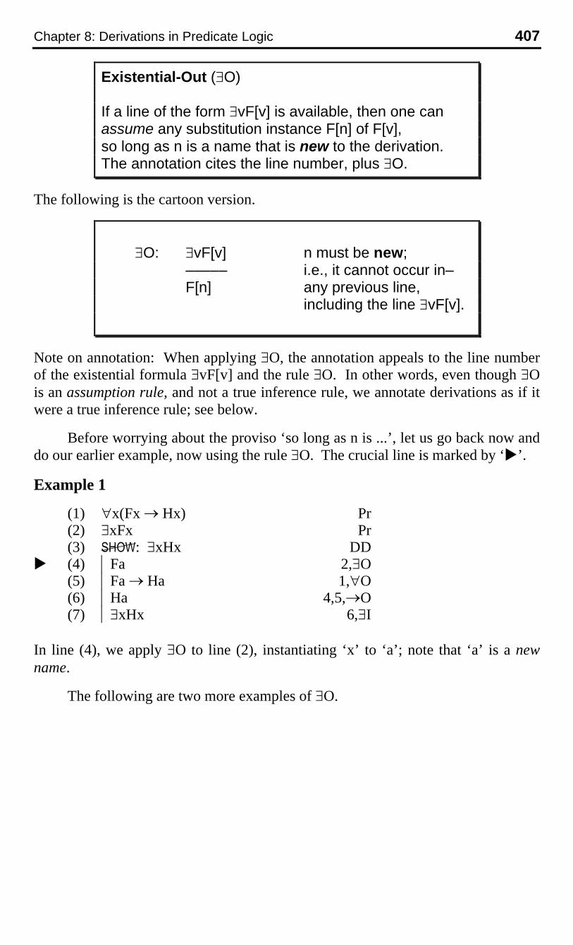
Existential-Out (∃O)
If a line of the form ∃vF[v] is available, then one canassume any substitution instance F[n] of F[v],so long as n is a name that is new to the derivation.The annotation cites the line number, plus ∃O.
The following is the cartoon version.
∃O: ∃vF[v] n must be new;––––– i.e., it cannot occur in–F[n] any previous line,
including the line ∃vF[v].
Note on annotation: When applying ∃O, the annotation appeals to the line numberof the existential formula ∃vF[v] and the rule ∃O. In other words, even though ∃Ois an assumption rule, and not a true inference rule, we annotate derivations as if itwere a true inference rule; see below.
Before worrying about the proviso ‘so long as n is ...’, let us go back now anddo our earlier example, now using the rule ∃O. The crucial line is marked by ‘u’.
Example 1
(1) ∀x(Fx → Hx) Pr(2) ∃xFx Pr(3) : ∃xHx DD
u (4) |Fa 2,∃O(5) |Fa → Ha 1,∀O(6) |Ha 4,5,→O(7) |∃xHx 6,∃I
In line (4), we apply ∃O to line (2), instantiating ‘x’ to ‘a’; note that ‘a’ is a newname.
The following are two more examples of ∃O.
408 Hardegree, Symbolic Logic
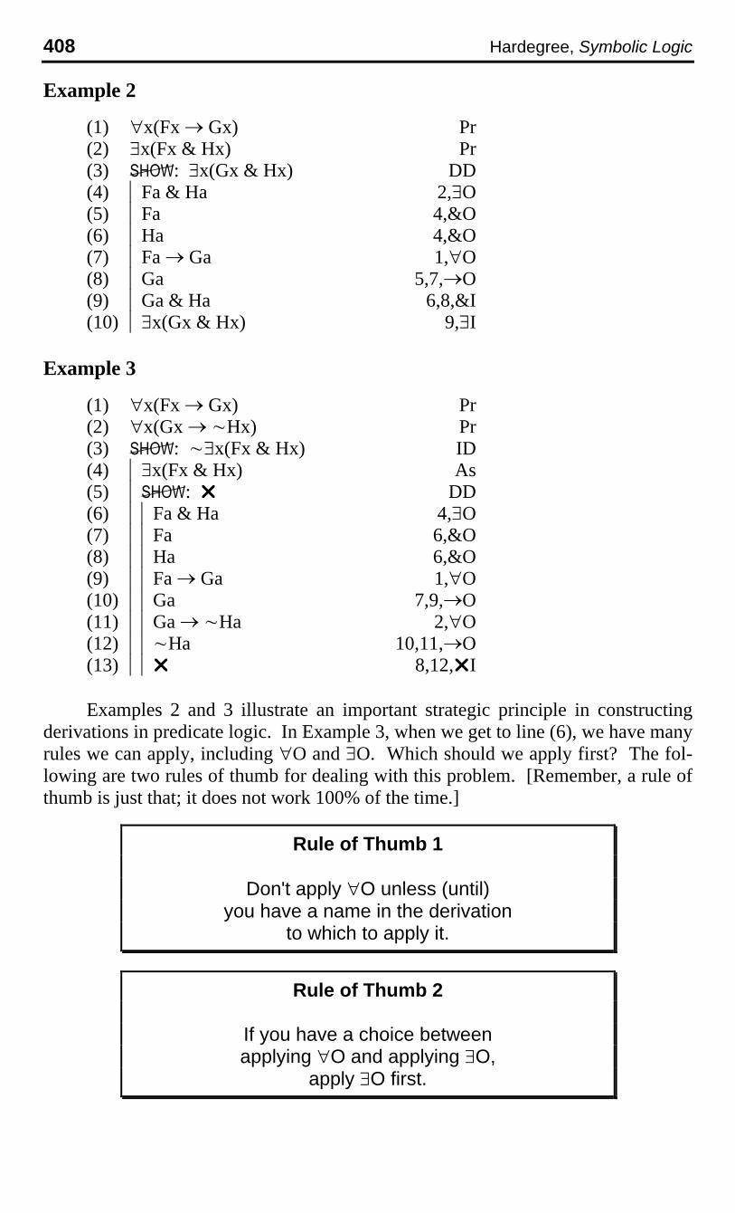
Example 2
(1) ∀x(Fx → Gx) Pr(2) ∃x(Fx & Hx) Pr(3) : ∃x(Gx & Hx) DD(4) |Fa & Ha 2,∃O(5) |Fa 4,&O(6) |Ha 4,&O(7) |Fa → Ga 1,∀O(8) |Ga 5,7,→O(9) |Ga & Ha 6,8,&I(10) |∃x(Gx & Hx) 9,∃I
Example 3
(1) ∀x(Fx → Gx) Pr(2) ∀x(Gx → ~Hx) Pr(3) : ~∃x(Fx & Hx) ID(4) |∃x(Fx & Hx) As(5) |: ¸ DD(6) ||Fa & Ha 4,∃O(7) ||Fa 6,&O(8) ||Ha 6,&O(9) ||Fa → Ga 1,∀O(10) ||Ga 7,9,→O(11) ||Ga → ~Ha 2,∀O(12) ||~Ha 10,11,→O(13) ||¸ 8,12,¸I
Examples 2 and 3 illustrate an important strategic principle in constructingderivations in predicate logic. In Example 3, when we get to line (6), we have manyrules we can apply, including ∀O and ∃O. Which should we apply first? The fol-lowing are two rules of thumb for dealing with this problem. [Remember, a rule ofthumb is just that; it does not work 100% of the time.]
Rule of Thumb 1
Don't apply ∀O unless (until)you have a name in the derivation
to which to apply it.
Rule of Thumb 2
If you have a choice betweenapplying ∀O and applying ∃O,
apply ∃O first.

Chapter 8: Derivations in Predicate Logic 409
The second rule is, in some sense, an application of the first rule. If one has noname to apply ∀O to, then one way to produce a name is to apply ∃O. Thus, onefirst applies ∃O, thus producing a name, and then applies ∀O.
What happens if you violate the above rules of thumb? Well, nothing verybad; you just end up with extraneous lines in the derivation. Consider the followingderivation, which contains a violation of Rules 1 and 2.
Example 2 (revisited):
(1) ∀x(Fx → Gx) Pr(2) ∃x(Fx & Hx) Pr(3) : ∃x(Gx & Hx) DD
u (*) |Fa → Ga 1,∀O(4) |Fb & Hb 2,∃O ‘b’ is new; ‘a’ isn't.(5) |Fb 4,&O(6) |Hb 4,&O(7) |Fb → Gb 1,∀O(8) |Gb 5,7,→O(9) |Gb & Hb 6,8,&I(10) |∃x(Gx & Hx) 9,∃I
The line marked ‘u’ is completely useless; it just gets in the way, as can be seenimmediately in line (4). This derivation is not incorrect; it would receive full crediton an exam (supposing it was assigned!); rather, it is somewhat disfigured.
In Examples 1-3, there are no names in the derivation except those introducedby ∃O. At the point we apply ∃O, there aren't any names in the derivation, so anyname will do! Thus, the requirement that the name be new is easy to satisfy.However, in other problems, additional names are involved, and the requirement isnot trivially satisfied.
Nonetheless, the requirement that the name be new is important, because itblocks erroneous derivations (and in particular, erroneous derivations of invalid ar-guments). Consider the following.
Invalid argument
(A) ∃xFx∃xGx/ ∃x(Fx & Gx)
at least one thing is Fat least one thing is G/ at least one thing is both F and G
There are many counterexamples to this argument; consider two of them.
Counterexamples
at least one number is evenat least one number is odd/ at least one number is both even and odd

410 Hardegree, Symbolic Logic
at least one person is femaleat least one person is male/ at least one person is both male and female
Argument (A) is clearly invalid. However, consider the following erroneousderivation.
Example 4 (erroneous derivation)
(1) ∃xFx Pr(2) ∃xGx Pr(3) ¬: ∃x(Fx & Gx) DD(4) Fa 1,∃O(5) Ga 2,∃O WRONG!!!(6) Fa & Ga 4,5,&I(7) ∃x(Fx & Gx) 6,∃I
The reason line (5) is wrong concerns the use of the name ‘a’, which is defi-nitely not new, since it appears in line (4). To be a proper application of ∃O, thename must be new, so we would have to instantiate Gx to Gb or Gc, anything butGa. When we correct line (5), the derivation looks like the following.
(1) ∃xFx Pr(2) ∃xGx Pr(3) ¬: ∃x(Fx & Gx) DD(4) Fa 1,∃O(5) Gb 2,∃O RIGHT!!!(6) ?????? ??? but we can't finish
Now, the derivation cannot be completed, but that is good, because the argument inquestion is, after all, invalid!
The previous examples do not involve multiply quantified formulas, so it isprobably a good idea to consider some of those.
Example 5
(1) ∀x(Fx → ∃yHy) Pr(2) : ∃xFx → ∃yHy CD(3) |∃xFx As(4) |: ∃yHy DD(5) ||Fa 3,∃O(6) ||Fa → ∃yHy 1,∀O(7) ||∃yHy 5,6,→O
As noted in the previous chapter, the premise may be read
if anything is F, then something is H,
whereas the conclusion may be read
if something is F, then something is H.
Chapter 8: Derivations in Predicate Logic 411
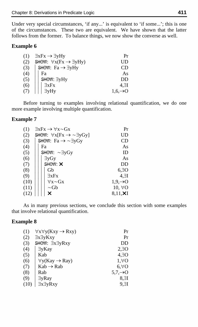
Under very special circumstances, ‘if any...’ is equivalent to ‘if some...’; this is oneof the circumstances. These two are equivalent. We have shown that the latterfollows from the former. To balance things, we now show the converse as well.
Example 6
(1) ∃xFx → ∃yHy Pr(2) : ∀x(Fx → ∃yHy) UD(3) |: Fa → ∃yHy CD(4) ||Fa As(5) ||: ∃yHy DD(6) |||∃xFx 4,∃I(7) |||∃yHy 1,6,→O
Before turning to examples involving relational quantification, we do onemore example involving multiple quantification.
Example 7
(1) ∃xFx → ∀x~Gx Pr(2) : ∀x[Fx → ~∃yGy] UD(3) |: Fa → ~∃yGy CD(4) ||Fa As(5) ||: ~∃yGy ID(6) |||∃yGy As(7) |||: ¸ DD(8) ||||Gb 6,∃O(9) ||||∃xFx 4,∃I(10) ||||∀x~Gx 1,9,→O(11) ||||~Gb 10, ∀O(12) ||||¸ 8,11,¸I
As in many previous sections, we conclude this section with some examplesthat involve relational quantification.
Example 8
(1) ∀x∀y(Kxy → Rxy) Pr(2) ∃x∃yKxy Pr(3) : ∃x∃yRxy DD(4) |∃yKay 2,∃O(5) |Kab 4,∃O(6) |∀y(Kay → Ray) 1,∀O(7) |Kab → Rab 6,∀O(8) |Rab 5,7,→O(9) |∃yRay 8,∃I(10) |∃x∃yRxy 9,∃I

412 Hardegree, Symbolic Logic
Example 9
(1) ∀x∃yRxy Pr(2) ∀x∀y[Rxy → Rxx] Pr(3) ∀x[Rxx → ∀yRyx] Pr(4) : ∀x∀yRxy UD(5) |: ∀yRay UD(6) ||: Rab DD(7) |||∃yRby 1,∀O(8) |||Rbc 7,∃O(9) |||∀y[Rby → Rbb] 2,∀O(10) |||Rbc → Rbb 9,∀O(11) |||Rbb 8,9,→O(12) |||Rbb → ∀yRyb 3,∀O(13) |||∀yRyb 11,12,→O(14) |||Rab 13,∀O
10. HOW EXISTENTIAL-OUT DIFFERSFROM THE OTHER RULES
As stated in the previous section, although we annotate existential-out just likeother elimination rules (like →O, ∨O, ∀O, etc.), it is not a true inference rule, but israther an assumption rule. In the present section, we show exactly how ∃O is dif-ferent from the other rules in predicate and sentential logic.
First consider a simple application of the rule ∀O.
∀xFx–––––Fa
This is a valid argument of predicate logic, and the corresponding derivation is triv-ial.
(1) ∀xFx Pr(2) : Fa DD(3) |Fa 2,∀O
Next, consider a simple application of the rule ∃I.
Fa–––––∃xFx
Again, the argument is valid, and the derivation is trivial.
Chapter 8: Derivations in Predicate Logic 413
(1) Fa Pr(2) : ∃xFx DD(3) |∃xFx 1,∃I
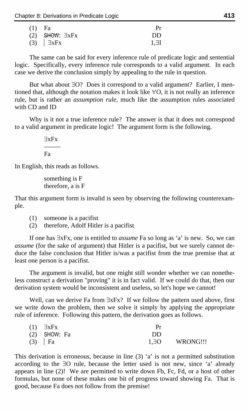
The same can be said for every inference rule of predicate logic and sententiallogic. Specifically, every inference rule corresponds to a valid argument. In eachcase we derive the conclusion simply by appealing to the rule in question.
But what about ∃O? Does it correspond to a valid argument? Earlier, I men-tioned that, although the notation makes it look like ∀O, it is not really an inferencerule, but is rather an assumption rule, much like the assumption rules associatedwith CD and ID
Why is it not a true inference rule? The answer is that it does not correspondto a valid argument in predicate logic! The argument form is the following.
∃xFx–––––Fa
In English, this reads as follows.
something is Ftherefore, a is F
That this argument form is invalid is seen by observing the following counterexam-ple.
(1) someone is a pacifist(2) therefore, Adolf Hitler is a pacifist
If one has ∃xFx, one is entitled to assume Fa so long as ‘a’ is new. So, we canassume (for the sake of argument) that Hitler is a pacifist, but we surely cannot de-duce the false conclusion that Hitler is/was a pacifist from the true premise that atleast one person is a pacifist.
The argument is invalid, but one might still wonder whether we can nonethe-less construct a derivation "proving" it is in fact valid. If we could do that, then ourderivation system would be inconsistent and useless, so let's hope we cannot!
Well, can we derive Fa from ∃xFx? If we follow the pattern used above, firstwe write down the problem, then we solve it simply by applying the appropriaterule of inference. Following this pattern, the derivation goes as follows.
(1) ∃xFx Pr(2) ¬: Fa DD(3) |Fa 1,∃O WRONG!!!
This derivation is erroneous, because in line (3) ‘a’ is not a permitted substitutionaccording to the ∃O rule, because the letter used is not new, since ‘a’ alreadyappears in line (2)! We are permitted to write down Fb, Fc, Fd, or a host of otherformulas, but none of these makes one bit of progress toward showing Fa. That isgood, because Fa does not follow from the premise!
414 Hardegree, Symbolic Logic
Thus, in spite of the notation, ∃O is quite different from the other rules. Whenwe apply ∃O to an existential formula (say, ∃xFx) to obtain a formula (say, Fc), weare not inferring or deducing Fc from ∃xFx. After all, this is not a valid inference.Rather, we are writing down an assumption. Some assumptions are permitted andsome are not; this is an example of a permitted assumption (provided, of course, thename is new) just like assuming the antecedent in conditional derivation.
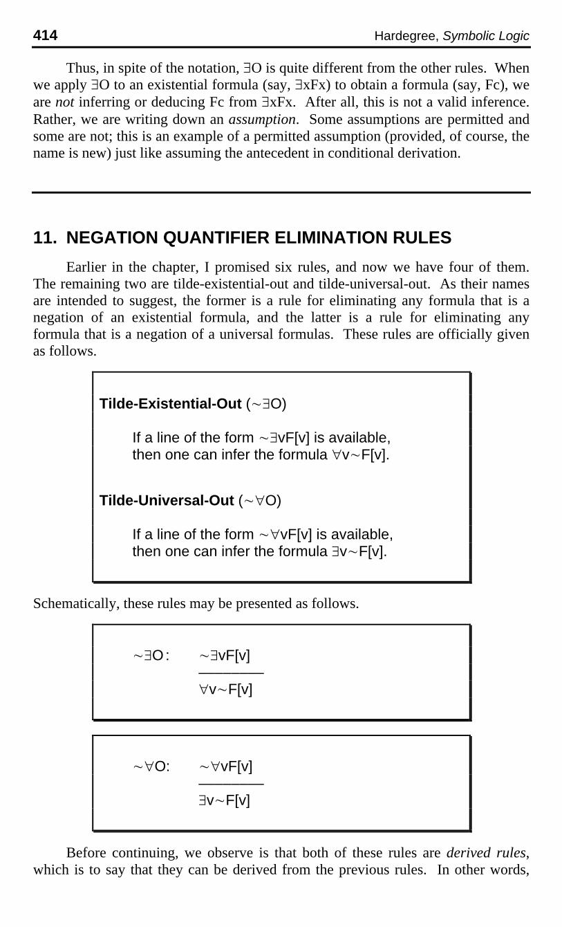
11. NEGATION QUANTIFIER ELIMINATION RULES
Earlier in the chapter, I promised six rules, and now we have four of them.The remaining two are tilde-existential-out and tilde-universal-out. As their namesare intended to suggest, the former is a rule for eliminating any formula that is anegation of an existential formula, and the latter is a rule for eliminating anyformula that is a negation of a universal formulas. These rules are officially givenas follows.
Tilde-Existential-Out (~∃O)
If a line of the form ~∃vF[v] is available,then one can infer the formula ∀v~F[v].
Tilde-Universal-Out (~∀O)
If a line of the form ~∀vF[v] is available,then one can infer the formula ∃v~F[v].
Schematically, these rules may be presented as follows.
~∃O: ~∃vF[v]––––––––∀v~F[v]
~∀O: ~∀vF[v]––––––––∃v~F[v]
Before continuing, we observe is that both of these rules are derived rules,which is to say that they can be derived from the previous rules. In other words,
Chapter 8: Derivations in Predicate Logic 415
these rules are completely dispensable: any conclusion that can be derived usingeither rule can be derived without using it. They are added for the sake of conven-ience.
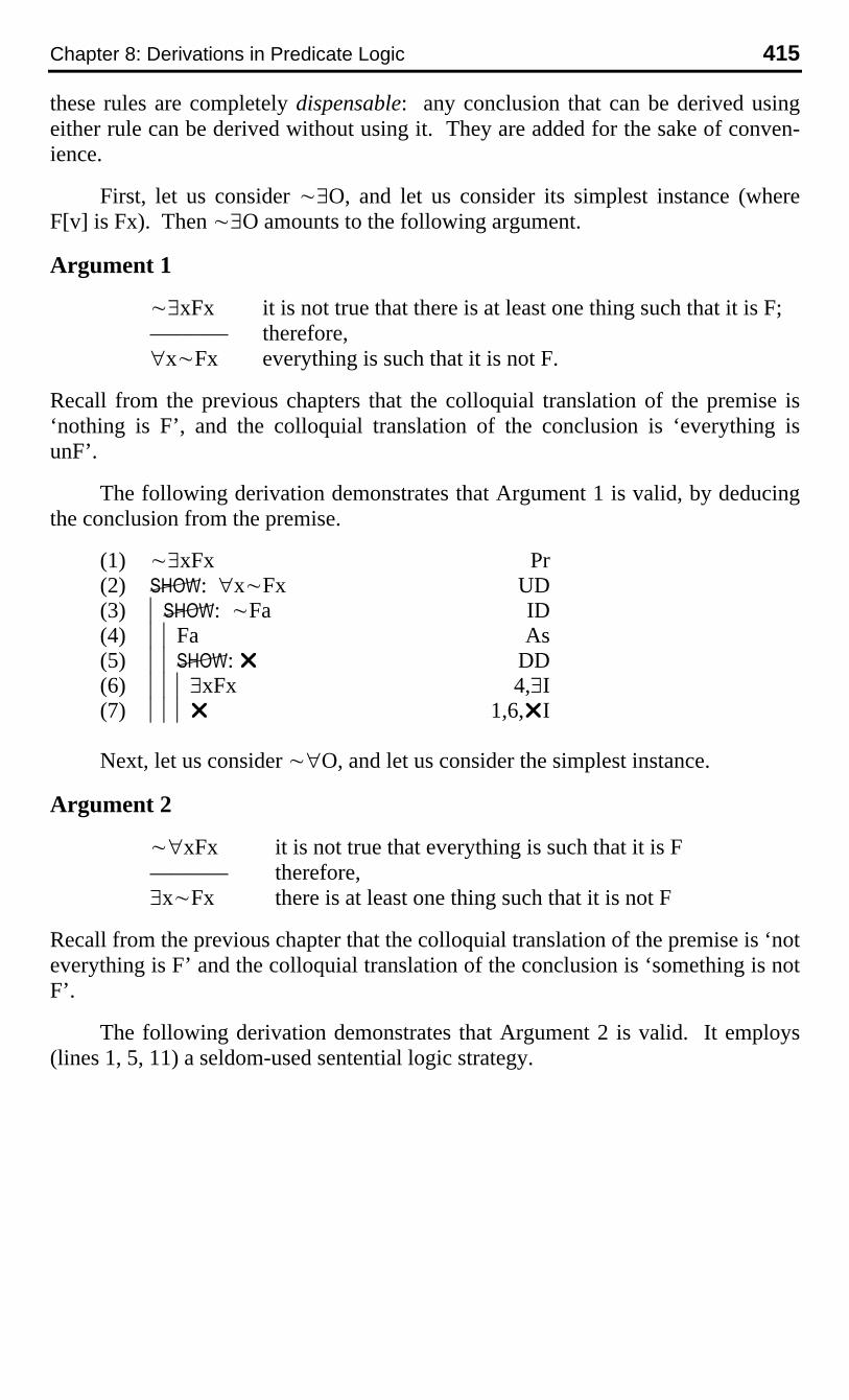
First, let us consider ~∃O, and let us consider its simplest instance (whereF[v] is Fx). Then ~∃O amounts to the following argument.
Argument 1
~∃xFx it is not true that there is at least one thing such that it is F;––––––– therefore,∀x~Fx everything is such that it is not F.
Recall from the previous chapters that the colloquial translation of the premise is‘nothing is F’, and the colloquial translation of the conclusion is ‘everything isunF’.
The following derivation demonstrates that Argument 1 is valid, by deducingthe conclusion from the premise.
(1) ~∃xFx Pr(2) : ∀x~Fx UD(3) |: ~Fa ID(4) ||Fa As(5) ||: ¸ DD(6) |||∃xFx 4,∃I(7) |||¸ 1,6,¸I
Next, let us consider ~∀O, and let us consider the simplest instance.
Argument 2
~∀xFx it is not true that everything is such that it is F––––––– therefore,∃x~Fx there is at least one thing such that it is not F
Recall from the previous chapter that the colloquial translation of the premise is ‘noteverything is F’ and the colloquial translation of the conclusion is ‘something is notF’.
The following derivation demonstrates that Argument 2 is valid. It employs(lines 1, 5, 11) a seldom-used sentential logic strategy.

416 Hardegree, Symbolic Logic
u (1) ~∀xFx Pr(2) : ∃x~Fx ID(3) |~∃x~Fx As(4) |: ¸ DD
u (5) ||: ∀xFx UD(6) |||: Fa ID(7) ||||~Fa As(8) ||||: ¸ DD(9) |||||∃x~Fx 7,∃I(10) |||||¸ 3,9,¸I
u (11) ||¸ 1,5,¸I
In each derivation, we have only shown the simplest instance of the rule,where F[v] is Fx. However, the complicated instances are shown in precisely thesame manner. We can in principle show for any formula F[v] and variable v that∀v~F[v] follows from ~∃vF[v], and that ∃v~F[v] follows from ~∀vF[v].
Note that the converse arguments are also valid, as demonstrated by thefollowing derivations.
(1) ∀x~Fx Pr(2) : ~∃xFx ID(3) |∃xFx As(4) |: ¸ DD(5) ||Fa 3,∃O(6) ||~Fa 1,∀O(7) ||¸ 5,6,¸I
(1) ∃x~Fx Pr(2) : ~∀xFx ID(3) |∀xFx As(4) |: ¸ DD(5) ||~Fa 1,∃O(6) ||Fa 3,∀O(7) ||¸ 5,6,¸I
Note carefully, however, that neither of the converse arguments corresponds to anyrule in our system. In particular,
THERE IS NO RULE TILDE-EXISTENTIAL-IN.
THERE IS NO RULE TILDE-UNIVERSAL-IN.
The corresponding arguments are valid, and accordingly can be demonstrated in oursystem. However, they are not inference rules. As usual, not every valid argumentform corresponds to an inference rule. This is simply a choice we make – we only
Chapter 8: Derivations in Predicate Logic 417
have negation-connective elimination rules, and no negation-connectiveintroduction rules.
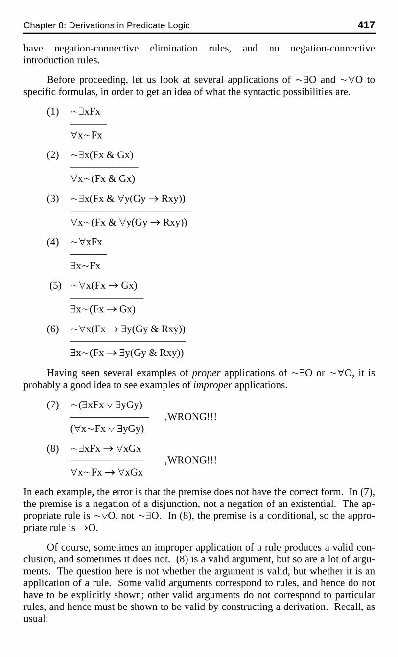
Before proceeding, let us look at several applications of ~∃O and ~∀O tospecific formulas, in order to get an idea of what the syntactic possibilities are.
(1) ~∃xFx–––––––∀x~Fx
(2) ~∃x(Fx & Gx)–––––––––––––∀x~(Fx & Gx)
(3) ~∃x(Fx & ∀y(Gy → Rxy))–––––––––––––––––––––––∀x~(Fx & ∀y(Gy → Rxy))
(4) ~∀xFx–––––––∃x~Fx
(5) ~∀x(Fx → Gx)––––––––––––––∃x~(Fx → Gx)
(6) ~∀x(Fx → ∃y(Gy & Rxy))––––––––––––––––––––––∃x~(Fx → ∃y(Gy & Rxy))
Having seen several examples of proper applications of ~∃O or ~∀O, it isprobably a good idea to see examples of improper applications.
(7) ~(∃xFx ∨ ∃yGy)––––––––––––––– ‚WRONG!!!(∀x~Fx ∨ ∃yGy)
(8) ~∃xFx → ∀xGx–––––––––––––– ‚WRONG!!!∀x~Fx → ∀xGx
In each example, the error is that the premise does not have the correct form. In (7),the premise is a negation of a disjunction, not a negation of an existential. The ap-propriate rule is ~∨O, not ~∃O. In (8), the premise is a conditional, so the appro-priate rule is →O.
Of course, sometimes an improper application of a rule produces a valid con-clusion, and sometimes it does not. (8) is a valid argument, but so are a lot of argu-ments. The question here is not whether the argument is valid, but whether it is anapplication of a rule. Some valid arguments correspond to rules, and hence do nothave to be explicitly shown; other valid arguments do not correspond to particularrules, and hence must be shown to be valid by constructing a derivation. Recall, asusual:

418 Hardegree, Symbolic Logic
INFERENCE RULES APPLYEXCLUSIVELY TO WHOLE LINES,
NOT TO PIECES OF LINES.
(8) is valid, so we can derive its conclusion from its premise. The following isone such derivation. It also illustrates a further point about our new rules.
Example 1
(1) ~∃xFx → ∀xGx Pr(2) : ∀x~Fx → ∀xGx CD(3) |∀x~Fx As
u (4) |: ∀xGx ID(5) ||~∀xGx As(6) ||: ¸ DD(7) |||~~∃xFx 1,5,→O(8) |||∃xFx 7,DN(9) |||Fa 8,∃O(10) |||~Fa 3,∀O(11) |||¸ 9,10,¸I
This derivation is curious in the following way: line (4) is shown by indirectderivation, rather than universal derivation. But this is permissible, since ID issuitable for any kind of formula.
Indeed, once we have the rule ~∀O, we can show any universal formula byID. By way of illustration, consider Example 2 from Section 7, first done usingUD, then done using ID.
Example 2 (done using UD)
(1) ∀x(Fx → Gx) Pr(2) : ∀xFx → ∀xGx CD(3) |∀xFx As
u (4) |: ∀xGx UD(5) ||: Ga DD(6) |||Fa → Ga 1,∀O(7) |||Fa 3,∀O(8) |||Ga 6,7,→O
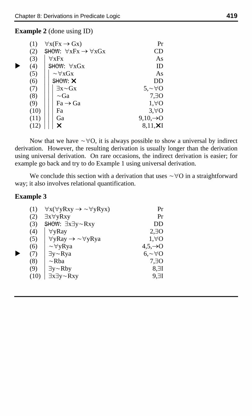
Chapter 8: Derivations in Predicate Logic 419
Example 2 (done using ID)
(1) ∀x(Fx → Gx) Pr(2) : ∀xFx → ∀xGx CD(3) |∀xFx As
u (4) |: ∀xGx ID(5) ||~∀xGx As(6) ||: ¸ DD(7) |||∃x~Gx 5,~∀O(8) |||~Ga 7,∃O(9) |||Fa → Ga 1,∀O(10) |||Fa 3,∀O(11) |||Ga 9,10,→O(12) |||¸ 8,11,¸I
Now that we have ~∀O, it is always possible to show a universal by indirectderivation. However, the resulting derivation is usually longer than the derivationusing universal derivation. On rare occasions, the indirect derivation is easier; forexample go back and try to do Example 1 using universal derivation.
We conclude this section with a derivation that uses ~∀O in a straightforwardway; it also involves relational quantification.
Example 3
(1) ∀x(∀yRxy → ~∀yRyx) Pr(2) ∃x∀yRxy Pr(3) : ∃x∃y~Rxy DD(4) |∀yRay 2,∃O(5) |∀yRay → ~∀yRya 1,∀O(6) |~∀yRya 4,5,→O
u (7) |∃y~Rya 6,~∀O(8) |~Rba 7,∃O(9) |∃y~Rby 8,∃I(10) |∃x∃y~Rxy 9,∃I
420 Hardegree, Symbolic Logic
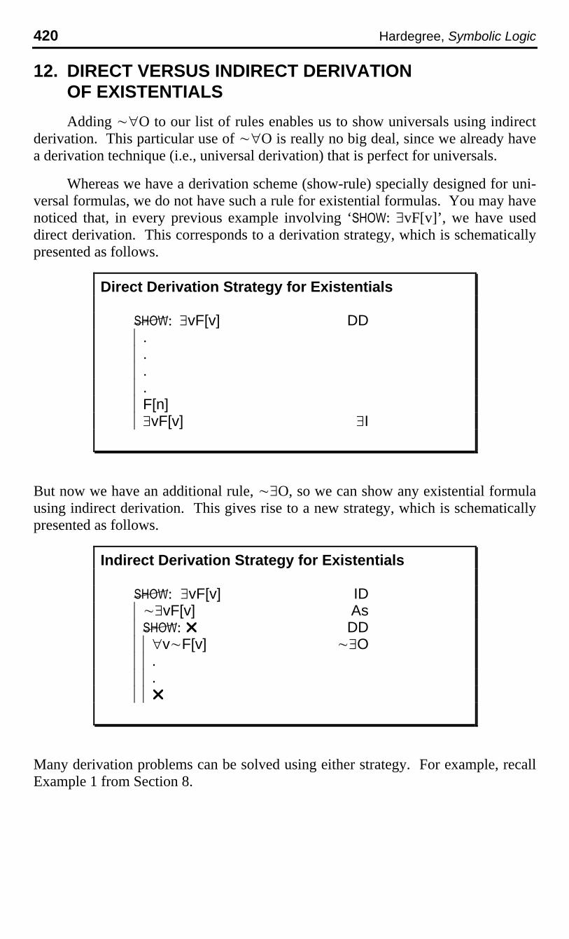
12. DIRECT VERSUS INDIRECT DERIVATIONOF EXISTENTIALS
Adding ~∀O to our list of rules enables us to show universals using indirectderivation. This particular use of ~∀O is really no big deal, since we already havea derivation technique (i.e., universal derivation) that is perfect for universals.
Whereas we have a derivation scheme (show-rule) specially designed for uni-versal formulas, we do not have such a rule for existential formulas. You may havenoticed that, in every previous example involving ‘¬: ∃vF[v]’, we have useddirect derivation. This corresponds to a derivation strategy, which is schematicallypresented as follows.
Direct Derivation Strategy for Existentials
: ∃vF[v] DD|.|.|.|.|F[n]|∃vF[v] ∃I
But now we have an additional rule, ~∃O, so we can show any existential formulausing indirect derivation. This gives rise to a new strategy, which is schematicallypresented as follows.
Indirect Derivation Strategy for Existentials
: ∃vF[v] ID|~∃vF[v] As|: ¸ DD||∀v~F[v] ~∃O||.||.||¸
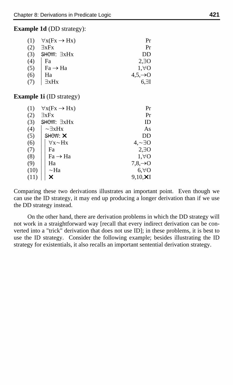
Many derivation problems can be solved using either strategy. For example, recallExample 1 from Section 8.
Chapter 8: Derivations in Predicate Logic 421
Example 1d (DD strategy):
(1) ∀x(Fx → Hx) Pr(2) ∃xFx Pr(3) : ∃xHx DD(4) |Fa 2,∃O(5) |Fa → Ha 1,∀O(6) |Ha 4,5,→O(7) |∃xHx 6,∃I
Example 1i (ID strategy)
(1) ∀x(Fx → Hx) Pr(2) ∃xFx Pr(3) : ∃xHx ID(4) |~∃xHx As(5) |: ¸ DD(6) ||∀x~Hx 4,~∃O(7) ||Fa 2,∃O(8) ||Fa → Ha 1,∀O(9) ||Ha 7,8,→O(10) ||~Ha 6,∀O(11) ||¸ 9,10,¸I
Comparing these two derivations illustrates an important point. Even though wecan use the ID strategy, it may end up producing a longer derivation than if we usethe DD strategy instead.
On the other hand, there are derivation problems in which the DD strategy willnot work in a straightforward way [recall that every indirect derivation can be con-verted into a "trick" derivation that does not use ID]; in these problems, it is best touse the ID strategy. Consider the following example; besides illustrating the IDstrategy for existentials, it also recalls an important sentential derivation strategy.

422 Hardegree, Symbolic Logic
Example 2
u (1) ∃xFx ∨ ∃xGx Pruu (2) : ∃x(Fx ∨ Gx) ID
(3) |~∃x(Fx ∨ Gx) As(4) |: ¸ DD(5) ||∀x~(Fx ∨ Gx) 3,~∃O
u (6) ||: ~∃xFx ID(7) |||∃xFx As(8) |||: ¸ DD(9) ||||Fa 7,∃O(10) ||||~(Fa ∨ Ga) 5,∀O(11) ||||~Fa 10,~∨O(12) ||||¸ 9,11,¸I
u (13) ||∃xGx 1,6,∨O(14) ||Gb 13,∃O(15) ||~(Fb ∨ Gb) 5,∀O(16) ||~Gb 15,~∨O(17) ||¸ 14,16,¸I
Recall the wedge-out strategy from sentential logic:
Wedge-Out Strategy
If you have a disjunction (for example, it is a premise),then you try to find (or show) the negation of one of thedisjuncts.
We are following the wedge-out strategy in line (6).
While we are on the topic of sentential derivation strategies, let us recall twoother strategies, the first being the wedge-derivation strategy, which isschematically presented as follows.
Wedge-Derivation Strategy
: A ∨ B ID|~(A ∨ B) As|: ¸ DD||~A ~∨O||~B ~∨O||.||.||.||¸ ¸I

Chapter 8: Derivations in Predicate Logic 423
This strategy is employed in the following example, which is the converse of 2.
Example 2c
(1) ∃x(Fx ∨ Gx) Pr(2) : ∃xFx ∨ ∃xGx ID(3) |~(∃xFx ∨ ∃xGx) As(4) |: ¸ DD(5) ||~∃xFx 3,~∨O(6) ||~∃xGx 3,~∨O(7) ||∀x~Fx 5,~∃O(8) ||∀x~Gx 6,~∃O(9) ||Fa ∨ Ga 1,∃O(10) ||~Fa 7,∀O(11) ||~Ga 8,∀O(12) ||Ga 9,10,∨O(13) ||¸ 11,12,¸I
Another sentential strategy is the arrow-out strategy, which is given asfollows.
Arrow-Out Strategy
If you have a conditional (for example, it is a premise),then you try to find (or show) either the antecedent orthe negation of the consequent.
The following example illustrates the arrow-out strategy; it also reiterates apoint made in Chapter 6 – namely, that an existential-conditional formula, e.g.,∃x(Fx → Gx), does not say much, and certainly does not say that some F is G.
424 Hardegree, Symbolic Logic
Example 3
u (1) ∀xFx → ∃xGx Pruu (2) : ∃x(Fx → Gx) ID
(3) |~∃x(Fx → Gx) As(4) |: ¸ DD(5) ||∀x~(Fx → Gx) 3,~∃O
u (6) ||: ∀xFx UD(7) |||: Fa DD(8) |||||~(Fa → Ga) 5,∀O(9) |||||Fa & ~Ga 8,~→O(10) |||||Fa 9,&O
u (11) ||∃xGx 1,6,→O(12) ||Gb 11,∃O(13) ||~(Fb → Gb) 5,∀O(14) ||Fb & ~Gb 13,~→O(15) ||~Gb 14,&O(16) ||¸ 12,15,¸I
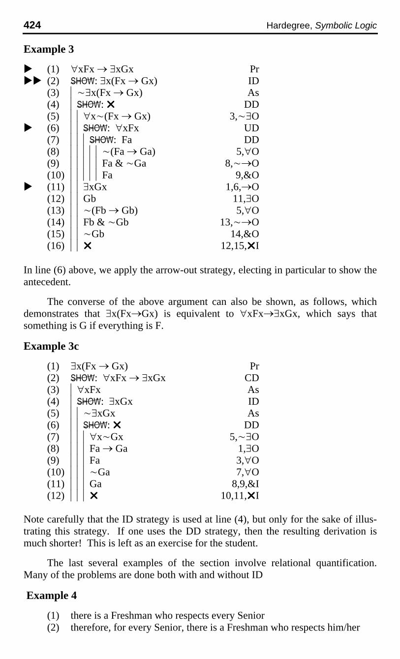
In line (6) above, we apply the arrow-out strategy, electing in particular to show theantecedent.
The converse of the above argument can also be shown, as follows, whichdemonstrates that ∃x(Fx→Gx) is equivalent to ∀xFx→∃xGx, which says thatsomething is G if everything is F.
Example 3c
(1) ∃x(Fx → Gx) Pr(2) : ∀xFx → ∃xGx CD(3) |∀xFx As(4) |: ∃xGx ID(5) ||~∃xGx As(6) ||: ¸ DD(7) |||∀x~Gx 5,~∃O(8) |||Fa → Ga 1,∃O(9) |||Fa 3,∀O(10) |||~Ga 7,∀O(11) |||Ga 8,9,&I(12) |||¸ 10,11,¸I
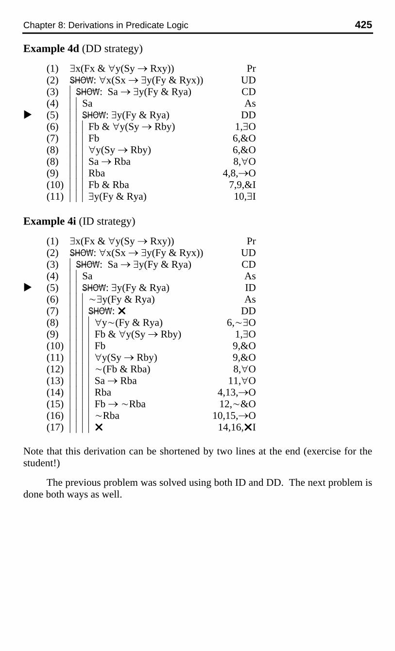
Note carefully that the ID strategy is used at line (4), but only for the sake of illus-trating this strategy. If one uses the DD strategy, then the resulting derivation ismuch shorter! This is left as an exercise for the student.
The last several examples of the section involve relational quantification.Many of the problems are done both with and without ID
Example 4
(1) there is a Freshman who respects every Senior(2) therefore, for every Senior, there is a Freshman who respects him/her
Chapter 8: Derivations in Predicate Logic 425
Example 4d (DD strategy)
(1) ∃x(Fx & ∀y(Sy → Rxy)) Pr(2) : ∀x(Sx → ∃y(Fy & Ryx)) UD(3) |: Sa → ∃y(Fy & Rya) CD(4) ||Sa As
u (5) ||: ∃y(Fy & Rya) DD(6) |||Fb & ∀y(Sy → Rby) 1,∃O(7) |||Fb 6,&O(8) |||∀y(Sy → Rby) 6,&O(8) |||Sa → Rba 8,∀O(9) |||Rba 4,8,→O(10) |||Fb & Rba 7,9,&I(11) |||∃y(Fy & Rya) 10,∃I
Example 4i (ID strategy)
(1) ∃x(Fx & ∀y(Sy → Rxy)) Pr(2) : ∀x(Sx → ∃y(Fy & Ryx)) UD(3) |: Sa → ∃y(Fy & Rya) CD(4) ||Sa As
u (5) ||: ∃y(Fy & Rya) ID(6) |||~∃y(Fy & Rya) As(7) |||: ¸ DD(8) ||||∀y~(Fy & Rya) 6,~∃O(9) ||||Fb & ∀y(Sy → Rby) 1,∃O(10) ||||Fb 9,&O(11) ||||∀y(Sy → Rby) 9,&O(12) ||||~(Fb & Rba) 8,∀O(13) ||||Sa → Rba 11,∀O(14) ||||Rba 4,13,→O(15) ||||Fb → ~Rba 12,~&O(16) ||||~Rba 10,15,→O(17) ||||¸ 14,16,¸I
Note that this derivation can be shortened by two lines at the end (exercise for thestudent!)
The previous problem was solved using both ID and DD. The next problem isdone both ways as well.

426 Hardegree, Symbolic Logic
Example 5
(1) there is someone who doesn't respect any Freshman(2) therefore, for every Freshman, there is someone who doesn't respect
him/her.
Example 5d (DD strategy)
(1) ∃x~∃y(Fy & Ryx) Pr(2) : ∀x(Fx → ∃y~Rxy) UD(3) |: Fa → ∃y~Ray CD(4) ||Fa As
u (5) ||: ∃y~Ray DD(6) |||~∃y(Fy & Ryb) 1,∃O(7) |||∀y~(Fy & Ryb) 6,~∃O(8) |||~(Fa & Rab) 7,∀O(9) |||Fa → ~Rab 8,~&O(10) |||~Rab 4,9,→O(11) |||∃y~Ray 10,∃I
Example 5i (ID strategy)
(1) ∃x~∃y(Fy & Ryx) Pr(2) : ∀x(Fx → ∃y~Rxy) UD(3) |: Fa → ∃y~Ray CD(4) ||Fa As
u (5) ||: ∃y~Ray ID(6) |||~∃y~Ray As(7) |||: ¸ DD(8) ||||∀y~~Ray 6,~∃O(9) ||||~∃y(Fy & Ryb) 1,∃O(10) ||||∀y~(Fy & Ryb) 9,~∃O(11) ||||~(Fa & Rab) 10,∀O(12) ||||Fa → ~Rab 11,~&O(12) ||||~~Rab 8,∀O(14) ||||~Fa 12,13,→O(15) ||||¸ 4,14,¸I
The final example of this section is considerably more complex than the previ-ous ones. It is done only once, using ID. Using the ID strategy is hard enough;using the DD strategy is also hard; try it and see!

Chapter 8: Derivations in Predicate Logic 427
Example 6
(1) every Freshman respects Adams(2) there is a Senior who doesn't respect any one who respects Adams(3) therefore, there is a Senior who doesn't respect any Freshman
(1) ∀x(Fx → Rxa) Pr(2) ∃x(Sx & ~∃y(Rya & Rxy)) Pr
u (3) : ∃x(Sx & ~∃y(Fy & Rxy)) ID(4) |~∃x(Sx & ~∃y(Fy & Rxy)) As(5) |: ¸ DD(6) ||∀x~(Sx & ~∃y(Fy & Rxy)) 4,~∃O(7) ||Sb & ~∃y(Rya & Rby) 2,∃O(8) ||Sb 7,&O(9) ||~∃y(Rya & Rby) 7,&O(10) ||∀y~(Rya & Rby) 9,~∃O(11) ||~(Sb & ~∃y(Fy & Rby)) 6,∀O(12) ||Sb → ~~∃y(Fy & Rby) 11,~&O(13) ||~~∃y(Fy & Rby) 8,12,→O(14) ||∃y(Fy & Rby) 13,DN(15) ||Fc & Rbc 14,∃O(16) ||Fc 15,&O(17) ||Rbc 15,&O(18) ||Fc → Rca 1,∀O(19) ||Rca 16,18,→O(20) ||~(Rca & Rbc) 10,∀O(21) ||Rca → ~Rbc 20,~&O(22) ||~Rbc 19,21,→O(23) ||¸ 17,22,¸I
What strategy should one employ in showing existential formulas? The fol-lowing principles might be useful in deciding between the two strategies.

428 Hardegree, Symbolic Logic
1. If any strategy will work, the ID strategy will. Theworst that can happen is that the derivation islonger than it needs to be.
2. If there are no names available, and if there are noexistential formulas to instantiate in order to obtainnames, then the ID strategy is advisable, althougha "trick" derivation is still possible.
3. When it works in a straightforward way (and itusually does), the DD strategy produces a prettierderivation. The worst that can happen is that onehas to start over, and use ID
4. If names are obtainable by applying ∃O, then theDD strategy will probably work; however, it mightbe harder than the ID strategy.
I conclude with the following principle, based on 1-4.
If you want a risk-free technique, use the ID strategy.
If you want more of a challenge, use the DD strategy.

Chapter 8: Derivations in Predicate Logic 429
13. APPENDIX 1: THE SYNTAX OF PREDICATE LOGIC
In this appendix, we review the syntactic features of predicate logic that arecrucial to understanding derivations in predicate logic. These include the followingnotions.
(1) principal (major) connective(2) free occurrence of a variable(3) substitution instance(4) alphabetic variant
1. OFFICIAL PRESENTATION OF THE SYNTAX OFPREDICATE LOGIC
A. Singular Terms.
1. Variables: x, y, z;2. Constants: a, b, c, ..., w;X. Nothing else is an singular term.
B. Predicate Letters.
0. 0-place predicate letters: A, B, ..., Z;1. 1-place predicate letters: the same;2. 2-place predicate letters: the same;3. 3-place predicate letters: the same;
and so forth...X. Nothing else is a predicate letter.
C. Quantifiers.
1. Universal Quantifiers: ∀x, ∀y, ∀z.2. Existential Quantifiers: ∃x, ∃y, ∃z.X. Nothing else is a quantifier.
D. Atomic Formulas.
1. If P is an n-place predicate letter, and t1,...,tn are singular terms, thenPt1...t2 is an atomic formula.
X. Nothing else is an atomic formula.
E. Formulas.
1. Every atomic formula is a formula.2. If A is a formula, then so is ~A.3. If A and B are formulas, then so are:
(a) (A & B)(b) (A ∨ B)(c) (A → B)(d) (A ↔ B).

430 Hardegree, Symbolic Logic
4. If A is a formula, then so are:∀xA, ∀yA, ∀zA,∃xA, ∃yA, ∃zA.
X. Nothing else is a formula.
Given the above characterization of the syntax of predicate logic, we see thatevery formula is exactly one of the following.
1. An atomic formula; there are no connectives:
Fa, Fx, Rab, Rax, Rxb, etc.
2. A negation; the major connective is negation:
~Fa, ~Rxy, ~(Fx & Gx), ~∀xFx, ~∃x∀yRxy, ~∀x(Fx → Gx), etc.
3. A universal; the major connective is a universal quantifier:
∀xFx, ∀yRay, ∀x(Fx → Gx), ∀x∃yRxy, ∀x(Fx → ∃yRxy), etc.
4. An existential; the major connective is an existential quantifier:
∃zFz, ∃xRax, ∃x(Fx & Gx), ∃y∀xRxy, ∃x(Fx & ∀yRyx), etc.
5. A conjunction; the major connective is ampersand:
Fx & Gy, ∀xFx & ∃yGy, ∀x(Fx → Gx) & ~∀x(Gx → Fx), etc.Fx ∨ Gy, ∀xFx ∨ ∃yGy, ∀x(Fx → Gx) ∨ ~∀x(Gx → Fx), etc.
6. A conditional; the major connective is arrow:
Fx → Gx, ∀xFx → ∀xGx, ∀x(Fx → Gx) → ∀x(Fx → Hx), etc.
7. A biconditional; the major connective is double-arrow:
Fx ↔ Gy, ∀xFx ↔ ∃yGy, ∀x(Fx → Gx) ↔ ~∀xGx, etc.
Now, just as in sentential logic, whether a rule of predicate logic applies to agiven formula is primarily determined by what the formula's major connective is.(In the case of negations, the immediately subordinate formula must also beconsidered.) So it is important to be able to recognize the major connective of aformula of predicate logic.
2. FREEDOM AND BONDAGE
A. Variables versus Occurrences of Variables.
How many words are there in this paragraph? Well, it depends on what youmean. This question is actually ambiguous between the following two differentquestions. (1) How many different (unique) words are used in this paragraph? (2)How long is this paragraph in words, or how many word occurrences are there in

Chapter 8: Derivations in Predicate Logic 431
this paragraph? The answer to the first question is: 46. On the other hand, theanswer to the second question is: 93. For example, the word ‘the’ appears 10times; which is to say that there are 10 occurrences of the word ‘the’ in thisparagraph.
Just as a given word of English (e.g., ‘the’) can occur many times in a givensentence (or paragraph) of English, a given logic symbol can occur many times in agiven formula. And in particular, a given variable can occur many times in a for-mula. Consider the following examples of occurrences of variables.
(1) Fx
‘x’ occurs once [or: there is one occurrence of ‘x’.]
(2) Rxy
‘x’ occurs once; ‘y’ occurs once.
(3) Fx → Hx
‘x’ occurs twice.
(4) ∀x(Fx → Hx)
‘x’ occurs three times.
(5) ∀y(Fx → Hy)
‘x’ occurs once; ‘y’ occurs twice.
(6) ∀x(Fx → ∀xHx)
‘x’ occurs four times.
(7) ∀x∀y(Rxy → Ryx)
‘x’ occurs three times; ‘y’ occurs three times.
We also speak the same way about occurrences of other symbols and combi-nations of symbols. So, for example, we can speak of occurrences of ‘~’, or occur-rences of ‘∀x’.
B. Quantifier Scope.
Definition
The scope of an occurrence of a quantifier is, bydefinition, the smallest formula containing that occur-rence.
The scope of a quantifier is exactly analogous to the scope of a negation sign in aformula of sentential logic. Consider the analogous definition.

432 Hardegree, Symbolic Logic
Definition
The scope of an occurrence of ‘~’ is, by definition, thesmallest formula containing that occurrence.
Examples
(1) ~P → Q; the scope of ~ is: ~P;(2) ~(P → Q);the scope of ~ is: ~(P → Q);(3) P → ~(R→S); the scope of ~ is: ~(R → S).
By analogy, consider the following involving universal quantifiers.
(1) ∀xFx → Fa the scope of ∀x is: ∀xFx(2) ∀x(Fx → Gx) the scope of ∀x is: ∀x(Fx → Gx)(3) Fa → ∀x(Gx→Hx) the scope of ∀x is: ∀x(Gx → Hx)
As a somewhat more complicated example, consider the following.
(4) ∀x(∀yRxy → ∀zRzx)
the scope of ∀x is ∀x(∀yRxy → ∀zRzx)the scope of ∀y is ∀yRxythe scope of ∀z is ∀zRzx
As a still more complicated example, consider the following.
(5) ∀x[∀xFx → ∀y(∀yGy → ∀zRxyz)];
the scope of the first ∀x is the whole formula;the scope of the second ∀x is ∀xFx;the scope of the first ∀y is ∀y(∀yGy → ∀zRxyz);the scope of the second ∀y is ∀yGy;the scope of the only ∀z is ∀zRxyz.
C. Government and Binding
Definition
‘∀x’ and ‘∃x’ govern the variable ‘x’;‘∀y’ and ‘∃y’ govern the variable ‘y’;‘∀z’ and ‘∃z’ govern the variable ‘z’;etc.
Chapter 8: Derivations in Predicate Logic 433
Definition
An occurrence of a quantifier binds an occurrence of avariable iff:
(1) the quantifier governs the variable,and
(2) the occurrence of the variable iscontained within the scope of theoccurrence of the quantifier.
Definition
An occurrence of a quantifier truly binds an occurrenceof a variable iff:
(1) the occurrence of the quantifier bindsthe occurrence of the variable,
and(2) the occurrence of the quantifier is inside
the scope of every occurrence of thatquantifier that binds the occurrence ofthe variable.
Example
∀x(Fx → ∀xGx);
In this formula the first ‘∀x’ binds every occurrence of ‘x’, but it only trulybinds the first two occurrences; on the other hand, the second ‘∀x’ truly binds thelast two occurrences of ‘x’.
D. Free versus Bound Occurrences of Variables
Every given occurrence of a given variable is either free or bound.
Definition
An occurrence of a variable in a formula F is bound in Fif and only if that occurrence is bound by somequantifier occurrence in F.
Definition
An occurrence of a variable in a formula F is free in F ifand only if that occurrence is not bound in F.
434 Hardegree, Symbolic Logic
Examples
(1) Fx:
the one and only occurrence of ‘x’ is free in this formula;
(2) ∀x(Fx → Gx):
all three occurrences of ‘x’ are bound by ‘∀x’;
(3) Fx → ∀xGx:
the first occurrence of ‘x’ is free; the remaining two occurrences arebound.
(4) ∀x(Fx → ∀xGx):
the first two occurrences of ‘x’ are bound by the first ‘∀x’; the secondtwo are bound by the second ‘∀x’.
(5) ∀x(∀yRxy → ∀zRzx):
every occurrence of every variable is bound.
Notice in example (4) that the variable ‘x’ occurs within the scope of two differentoccurrences of ‘∀x’. It is only the innermost occurrence of ‘∀x’ that truly binds thevariable, however. The other occurrence of ‘∀x’ binds the first occurrence of ‘x’but none of the remaining ones.
3. SUBSTITUTION INSTANCES
Having described the difference between free and bound occurrences of vari-ables, we turn to the topic of substitution instance, which is officially defined asfollows.
Definition
Let v be any variable, let F[v] be any formula containingv, and let n be any name. Then a substitution instanceof the formula F[v] is any formula F[n] obtained fromF[v] by substituting occurrences of the name n for eachand every occurrence of the variable v that is free inF[v].
Let us look at a few examples; in each example, I give examples of correct substitu-tion instances, and then I give examples of incorrect substitution instances.
(1) Fx:
Correct: Fa; Fb; Fc; etc.;Incorrect: Fx; Fy, Fz.
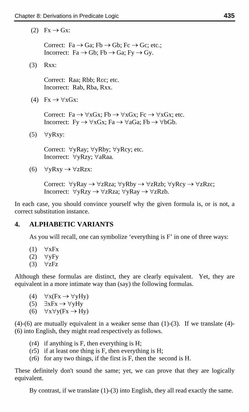
Chapter 8: Derivations in Predicate Logic 435
(2) Fx → Gx:
Correct: Fa → Ga; Fb → Gb; Fc → Gc; etc.;Incorrect: Fa → Gb; Fb → Ga; Fy → Gy.
(3) Rxx:
Correct: Raa; Rbb; Rcc; etc.Incorrect: Rab, Rba, Rxx.
(4) Fx → ∀xGx:
Correct: Fa → ∀xGx; Fb → ∀xGx; Fc → ∀xGx; etc.Incorrect: Fy → ∀xGx; Fa → ∀aGa; Fb → ∀bGb.
(5) ∀yRxy:
Correct: ∀yRay; ∀yRby; ∀yRcy; etc.Incorrect: ∀yRzy; ∀aRaa.
(6) ∀yRxy → ∀zRzx:
Correct: ∀yRay → ∀zRza; ∀yRby → ∀zRzb; ∀yRcy → ∀zRzc;Incorrect: ∀yRzy → ∀zRza; ∀yRay → ∀zRzb.
In each case, you should convince yourself why the given formula is, or is not, acorrect substitution instance.
4. ALPHABETIC VARIANTS
As you will recall, one can symbolize ‘everything is F’ in one of three ways:
(1) ∀xFx(2) ∀yFy(3) ∀zFz
Although these formulas are distinct, they are clearly equivalent. Yet, they areequivalent in a more intimate way than (say) the following formulas.
(4) ∀x(Fx → ∀yHy)(5) ∃xFx → ∀yHy(6) ∀x∀y(Fx → Hy)
(4)-(6) are mutually equivalent in a weaker sense than (1)-(3). If we translate (4)-(6) into English, they might read respectively as follows.
(r4) if anything is F, then everything is H;(r5) if at least one thing is F, then everything is H;(r6) for any two things, if the first is F, then the second is H.
These definitely don't sound the same; yet, we can prove that they are logicallyequivalent.
By contrast, if we translate (1)-(3) into English, they all read exactly the same.
436 Hardegree, Symbolic Logic
(r1-3) everything is F.
We describe the relation between the various (1)-(3) by saying that they are alpha-betic variants of one another. They are slightly different symbolic ways of sayingexactly the same thing.
The formal definition of alphabetic variants is difficult to give in the general case ofunlimited variables. But if we restrict ourselves to just three variables, then thedefinition is merely complicated.
Definition
A formula F is closed iff: no variable occurs free in F.
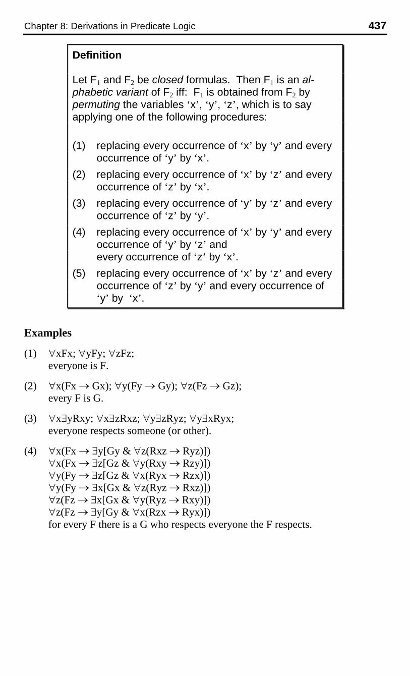
Chapter 8: Derivations in Predicate Logic 437
Definition
Let F1 and F2 be closed formulas. Then F1 is an al-phabetic variant of F2 iff: F1 is obtained from F2 bypermuting the variables ‘x’, ‘y’, ‘z’, which is to sayapplying one of the following procedures:
(1) replacing every occurrence of ‘x’ by ‘y’ and everyoccurrence of ‘y’ by ‘x’.
(2) replacing every occurrence of ‘x’ by ‘z’ and everyoccurrence of ‘z’ by ‘x’.
(3) replacing every occurrence of ‘y’ by ‘z’ and everyoccurrence of ‘z’ by ‘y’.
(4) replacing every occurrence of ‘x’ by ‘y’ and everyoccurrence of ‘y’ by ‘z’ andevery occurrence of ‘z’ by ‘x’.
(5) replacing every occurrence of ‘x’ by ‘z’ and everyoccurrence of ‘z’ by ‘y’ and every occurrence of‘y’ by ‘x’.
Examples
(1) ∀xFx; ∀yFy; ∀zFz;everyone is F.
(2) ∀x(Fx → Gx); ∀y(Fy → Gy); ∀z(Fz → Gz);every F is G.
(3) ∀x∃yRxy; ∀x∃zRxz; ∀y∃zRyz; ∀y∃xRyx;everyone respects someone (or other).
(4) ∀x(Fx → ∃y[Gy & ∀z(Rxz → Ryz)])∀x(Fx → ∃z[Gz & ∀y(Rxy → Rzy)])∀y(Fy → ∃z[Gz & ∀x(Ryx → Rzx)])∀y(Fy → ∃x[Gx & ∀z(Ryz → Rxz)])∀z(Fz → ∃x[Gx & ∀y(Ryz → Rxy)])∀z(Fz → ∃y[Gy & ∀x(Rzx → Ryx)])for every F there is a G who respects everyone the F respects.

438 Hardegree, Symbolic Logic
14. APPENDIX 2: SUMMARY OF RULES FORSYSTEM PL (PREDICATE LOGIC)
A. Sentential Logic Rules
Every rule of SL (sentential logic) is also a rule of PL (predicate logic).
B. Rules that don't require a new name
In the following, v is any variable, a and n are names, F[v] is a formula.Furthermore, F[a] is the formula that results when a is substituted for v at allits free occurrences, and similarly, F[n] is the formula that results when n is sosubstituted.
Universal-Out (∀∀O)
∀vF[v]––––––F[a] a can be any name
Existential-In (∃∃I)
F[a] a can be any name––––––∃vF[v]
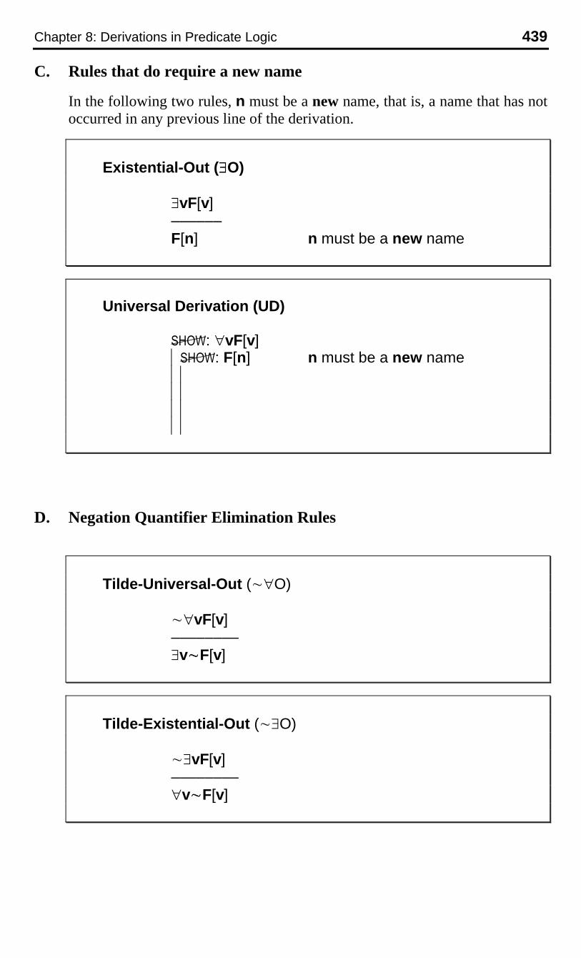
Chapter 8: Derivations in Predicate Logic 439
C. Rules that do require a new name
In the following two rules, n must be a new name, that is, a name that has notoccurred in any previous line of the derivation.
Existential-Out (∃∃O)
∃vF[v]––––––F[n] n must be a new name
Universal Derivation (UD)
: ∀vF[v]|: F[n] n must be a new name||||||||
D. Negation Quantifier Elimination Rules
Tilde-Universal-Out (~∀O)
~∀vF[v]––––––––∃v~~F[v]
Tilde-Existential-Out (~∃O)
~∃vF[v]––––––––∀v~~F[v]
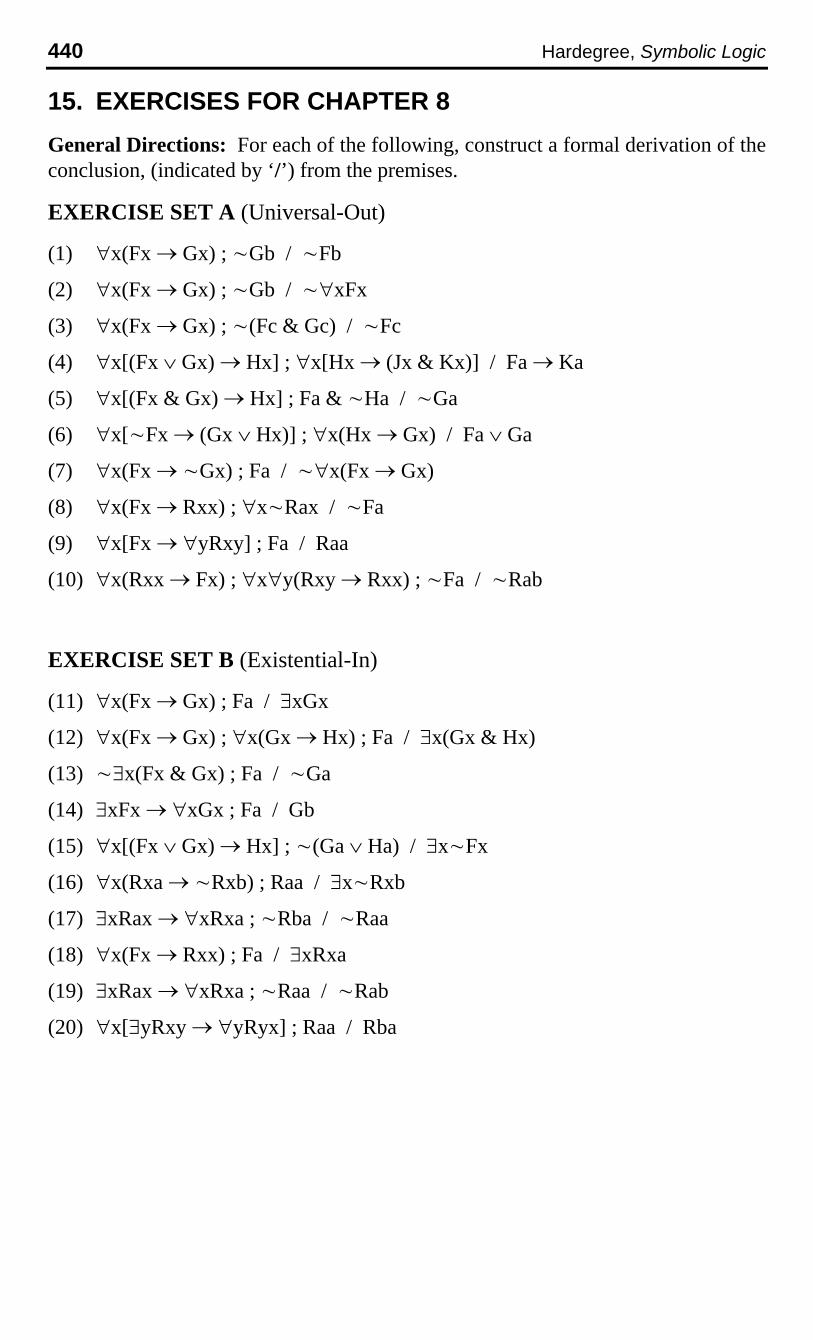
440 Hardegree, Symbolic Logic
15. EXERCISES FOR CHAPTER 8
General Directions: For each of the following, construct a formal derivation of theconclusion, (indicated by ‘/’) from the premises.
EXERCISE SET A (Universal-Out)
(1) ∀x(Fx → Gx) ; ~Gb / ~Fb
(2) ∀x(Fx → Gx) ; ~Gb / ~∀xFx
(3) ∀x(Fx → Gx) ; ~(Fc & Gc) / ~Fc
(4) ∀x[(Fx ∨ Gx) → Hx] ; ∀x[Hx → (Jx & Kx)] / Fa → Ka
(5) ∀x[(Fx & Gx) → Hx] ; Fa & ~Ha / ~Ga
(6) ∀x[~Fx → (Gx ∨ Hx)] ; ∀x(Hx → Gx) / Fa ∨ Ga
(7) ∀x(Fx → ~Gx) ; Fa / ~∀x(Fx → Gx)
(8) ∀x(Fx → Rxx) ; ∀x~Rax / ~Fa
(9) ∀x[Fx → ∀yRxy] ; Fa / Raa
(10) ∀x(Rxx → Fx) ; ∀x∀y(Rxy → Rxx) ; ~Fa / ~Rab
EXERCISE SET B (Existential-In)
(11) ∀x(Fx → Gx) ; Fa / ∃xGx
(12) ∀x(Fx → Gx) ; ∀x(Gx → Hx) ; Fa / ∃x(Gx & Hx)
(13) ~∃x(Fx & Gx) ; Fa / ~Ga
(14) ∃xFx → ∀xGx ; Fa / Gb
(15) ∀x[(Fx ∨ Gx) → Hx] ; ~(Ga ∨ Ha) / ∃x~Fx
(16) ∀x(Rxa → ~Rxb) ; Raa / ∃x~Rxb
(17) ∃xRax → ∀xRxa ; ~Rba / ~Raa
(18) ∀x(Fx → Rxx) ; Fa / ∃xRxa
(19) ∃xRax → ∀xRxa ; ~Raa / ~Rab
(20) ∀x[∃yRxy → ∀yRyx] ; Raa / Rba

Chapter 8: Derivations in Predicate Logic 441
EXERCISE SET C (Universal Derivation)
(21) ∀x(Fx → Gx) ; ∀x(Gx → Hx) / ∀x(Fx → Hx)
(22) ∀x(Fx → Gx) ; ∀x[(Fx & Gx) → Hx] / ∀x(Fx → Hx)
(23) ∀x(Fx → Gx) ; ∀x([Gx ∨ Hx] → Kx) / ∀x(Fx → Kx)
(24) ∀xFx & ∀xGx / ∀x(Fx & Gx)
(25) ∀xFx ∨ ∀xGx / ∀x(Fx ∨ Gx)
(26) ~∃xFx / ∀x(Fx → Gx)
(27) ~∃x(Fx & Gx) / ∀x(Fx → ~Gx)
(28) ∀x(Fx → Gx) ; ~∃x(Gx & Hx) / ∀x(Fx → ~Hx)
(29) ∀x(Fx → Gx) / ∀xFx → ∀xGx
(30) ∀x((Fx & Gx) → Hx) / ∀x(Fx → Gx) → ∀x(Fx → Hx)
EXERCISE SET D (Existential-Out)
(31) ∀x(Fx → Gx) ; ∃x(Fx & Hx) / ∃x(Gx & Hx)
(32) ∃x(Fx & Gx) ; ∀x(Hx → ~Gx) / ∃x(Fx & ~Hx)
(33) ∀x(Fx → Gx) ; ∀x(Gx → Hx) ; ∃x~Hx / ∃x~Fx
(34) ∀x(Fx → ~Gx) / ~∃x(Fx & Gx)
(35) ∃x(Fx & ~Gx) / ~∀x(Fx → Gx)
(36) ∀x(Fx → Gx) ; ∀x(Gx → ~Hx) / ~∃x(Fx & Hx)
(37) ∀x(Gx → Hx) ; ∃x(Ix & ~Hx) ; ∀x(~Fx ∨ Gx) / ∃x(Ix & ~Fx)
(38) ∃xFx ∨ ∃xGx ; ∀x~Fx / ∃xGx
(39) ∀x(Fx → Gx) / ∃xFx → ∃xGx
(40) ∀x(Fx → (Gx → Hx)) / ∃x(Fx & Gx) → ∃x(Fx & Hx)
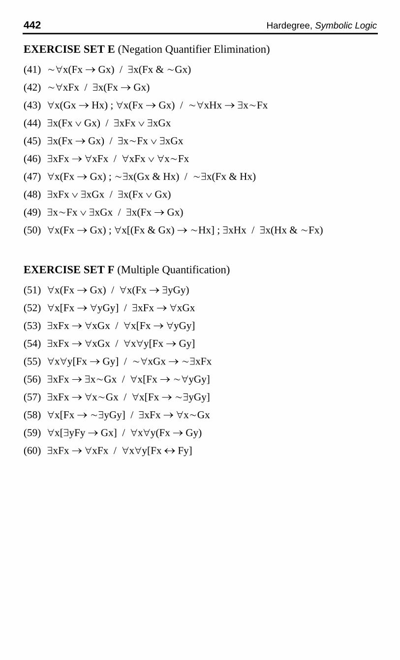
442 Hardegree, Symbolic Logic
EXERCISE SET E (Negation Quantifier Elimination)
(41) ~∀x(Fx → Gx) / ∃x(Fx & ~Gx)
(42) ~∀xFx / ∃x(Fx → Gx)
(43) ∀x(Gx → Hx) ; ∀x(Fx → Gx) / ~∀xHx → ∃x~Fx
(44) ∃x(Fx ∨ Gx) / ∃xFx ∨ ∃xGx
(45) ∃x(Fx → Gx) / ∃x~Fx ∨ ∃xGx
(46) ∃xFx → ∀xFx / ∀xFx ∨ ∀x~Fx
(47) ∀x(Fx → Gx) ; ~∃x(Gx & Hx) / ~∃x(Fx & Hx)
(48) ∃xFx ∨ ∃xGx / ∃x(Fx ∨ Gx)
(49) ∃x~Fx ∨ ∃xGx / ∃x(Fx → Gx)
(50) ∀x(Fx → Gx) ; ∀x[(Fx & Gx) → ~Hx] ; ∃xHx / ∃x(Hx & ~Fx)
EXERCISE SET F (Multiple Quantification)
(51) ∀x(Fx → Gx) / ∀x(Fx → ∃yGy)
(52) ∀x[Fx → ∀yGy] / ∃xFx → ∀xGx
(53) ∃xFx → ∀xGx / ∀x[Fx → ∀yGy]
(54) ∃xFx → ∀xGx / ∀x∀y[Fx → Gy]
(55) ∀x∀y[Fx → Gy] / ~∀xGx → ~∃xFx
(56) ∃xFx → ∃x~Gx / ∀x[Fx → ~∀yGy]
(57) ∃xFx → ∀x~Gx / ∀x[Fx → ~∃yGy]
(58) ∀x[Fx → ~∃yGy] / ∃xFx → ∀x~Gx
(59) ∀x[∃yFy → Gx] / ∀x∀y(Fx → Gy)
(60) ∃xFx → ∀xFx / ∀x∀y[Fx ↔ Fy]
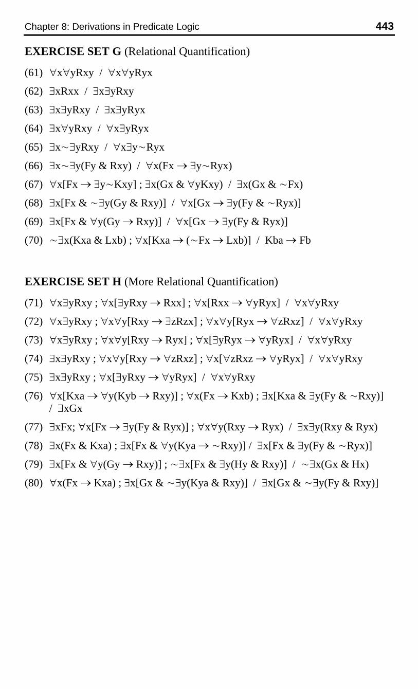
Chapter 8: Derivations in Predicate Logic 443
EXERCISE SET G (Relational Quantification)
(61) ∀x∀yRxy / ∀x∀yRyx
(62) ∃xRxx / ∃x∃yRxy
(63) ∃x∃yRxy / ∃x∃yRyx
(64) ∃x∀yRxy / ∀x∃yRyx
(65) ∃x~∃yRxy / ∀x∃y~Ryx
(66) ∃x~∃y(Fy & Rxy) / ∀x(Fx → ∃y~Ryx)
(67) ∀x[Fx → ∃y~Kxy] ; ∃x(Gx & ∀yKxy) / ∃x(Gx & ~Fx)
(68) ∃x[Fx & ~∃y(Gy & Rxy)] / ∀x[Gx → ∃y(Fy & ~Ryx)]
(69) ∃x[Fx & ∀y(Gy → Rxy)] / ∀x[Gx → ∃y(Fy & Ryx)]
(70) ~∃x(Kxa & Lxb) ; ∀x[Kxa → (~Fx → Lxb)] / Kba → Fb
EXERCISE SET H (More Relational Quantification)
(71) ∀x∃yRxy ; ∀x[∃yRxy → Rxx] ; ∀x[Rxx → ∀yRyx] / ∀x∀yRxy
(72) ∀x∃yRxy ; ∀x∀y[Rxy → ∃zRzx] ; ∀x∀y[Ryx → ∀zRxz] / ∀x∀yRxy
(73) ∀x∃yRxy ; ∀x∀y[Rxy → Ryx] ; ∀x[∃yRyx → ∀yRyx] / ∀x∀yRxy
(74) ∃x∃yRxy ; ∀x∀y[Rxy → ∀zRxz] ; ∀x[∀zRxz → ∀yRyx] / ∀x∀yRxy
(75) ∃x∃yRxy ; ∀x[∃yRxy → ∀yRyx] / ∀x∀yRxy
(76) ∀x[Kxa → ∀y(Kyb → Rxy)] ; ∀x(Fx → Kxb) ; ∃x[Kxa & ∃y(Fy & ~Rxy)]/ ∃xGx
(77) ∃xFx; ∀x[Fx → ∃y(Fy & Ryx)] ; ∀x∀y(Rxy → Ryx) / ∃x∃y(Rxy & Ryx)
(78) ∃x(Fx & Kxa) ; ∃x[Fx & ∀y(Kya → ~Rxy)] / ∃x[Fx & ∃y(Fy & ~Ryx)]
(79) ∃x[Fx & ∀y(Gy → Rxy)] ; ~∃x[Fx & ∃y(Hy & Rxy)] / ~∃x(Gx & Hx)
(80) ∀x(Fx → Kxa) ; ∃x[Gx & ~∃y(Kya & Rxy)] / ∃x[Gx & ~∃y(Fy & Rxy)]
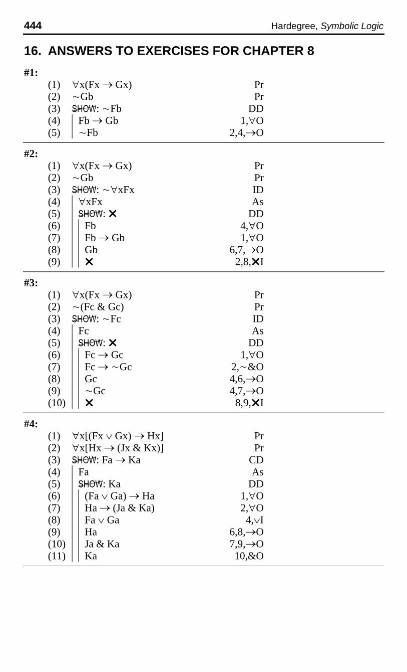
444 Hardegree, Symbolic Logic
16. ANSWERS TO EXERCISES FOR CHAPTER 8
#1:(1) ∀x(Fx → Gx) Pr(2) ~Gb Pr(3) : ~Fb DD(4) |Fb → Gb 1,∀O(5) |~Fb 2,4,→O
#2:(1) ∀x(Fx → Gx) Pr(2) ~Gb Pr(3) : ~∀xFx ID(4) |∀xFx As(5) |: ¸ DD(6) ||Fb 4,∀O(7) ||Fb → Gb 1,∀O(8) ||Gb 6,7,→O(9) ||¸ 2,8,¸I
#3:(1) ∀x(Fx → Gx) Pr(2) ~(Fc & Gc) Pr(3) : ~Fc ID(4) |Fc As(5) |: ¸ DD(6) ||Fc → Gc 1,∀O(7) ||Fc → ~Gc 2,~&O(8) ||Gc 4,6,→O(9) ||~Gc 4,7,→O(10) ||¸ 8,9,¸I
#4:(1) ∀x[(Fx ∨ Gx) → Hx] Pr(2) ∀x[Hx → (Jx & Kx)] Pr(3) : Fa → Ka CD(4) |Fa As(5) |: Ka DD(6) ||(Fa ∨ Ga) → Ha 1,∀O(7) ||Ha → (Ja & Ka) 2,∀O(8) ||Fa ∨ Ga 4,∨I(9) ||Ha 6,8,→O(10) ||Ja & Ka 7,9,→O(11) ||Ka 10,&O
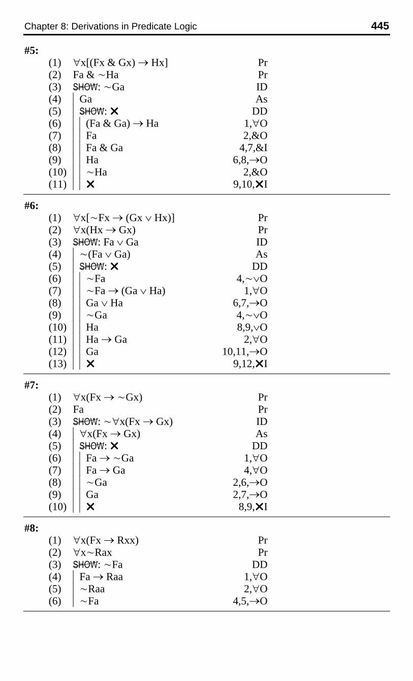
Chapter 8: Derivations in Predicate Logic 445
#5:(1) ∀x[(Fx & Gx) → Hx] Pr(2) Fa & ~Ha Pr(3) : ~Ga ID(4) |Ga As(5) |: ¸ DD(6) ||(Fa & Ga) → Ha 1,∀O(7) ||Fa 2,&O(8) ||Fa & Ga 4,7,&I(9) ||Ha 6,8,→O(10) ||~Ha 2,&O(11) ||¸ 9,10,¸I
#6:(1) ∀x[~Fx → (Gx ∨ Hx)] Pr(2) ∀x(Hx → Gx) Pr(3) : Fa ∨ Ga ID(4) |~(Fa ∨ Ga) As(5) |: ¸ DD(6) ||~Fa 4,~∨O(7) ||~Fa → (Ga ∨ Ha) 1,∀O(8) ||Ga ∨ Ha 6,7,→O(9) ||~Ga 4,~∨O(10) ||Ha 8,9,∨O(11) ||Ha → Ga 2,∀O(12) ||Ga 10,11,→O(13) ||¸ 9,12,¸I
#7:(1) ∀x(Fx → ~Gx) Pr(2) Fa Pr(3) : ~∀x(Fx → Gx) ID(4) |∀x(Fx → Gx) As(5) |: ¸ DD(6) ||Fa → ~Ga 1,∀O(7) ||Fa → Ga 4,∀O(8) ||~Ga 2,6,→O(9) ||Ga 2,7,→O(10) ||¸ 8,9,¸I
#8:(1) ∀x(Fx → Rxx) Pr(2) ∀x~Rax Pr(3) : ~Fa DD(4) |Fa → Raa 1,∀O(5) |~Raa 2,∀O(6) |~Fa 4,5,→O
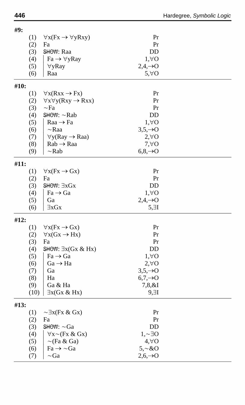
446 Hardegree, Symbolic Logic
#9:(1) ∀x(Fx → ∀yRxy) Pr(2) Fa Pr(3) : Raa DD(4) |Fa → ∀yRay 1,∀O(5) |∀yRay 2,4,→O(6) |Raa 5,∀O
#10:(1) ∀x(Rxx → Fx) Pr(2) ∀x∀y(Rxy → Rxx) Pr(3) ~Fa Pr(4) : ~Rab DD(5) |Raa → Fa 1,∀O(6) |~Raa 3,5,→O(7) |∀y(Ray → Raa) 2,∀O(8) |Rab → Raa 7,∀O(9) |~Rab 6,8,→O
#11:(1) ∀x(Fx → Gx) Pr(2) Fa Pr(3) : ∃xGx DD(4) |Fa → Ga 1,∀O(5) |Ga 2,4,→O(6) |∃xGx 5,∃I
#12:(1) ∀x(Fx → Gx) Pr(2) ∀x(Gx → Hx) Pr(3) Fa Pr(4) : ∃x(Gx & Hx) DD(5) |Fa → Ga 1,∀O(6) |Ga → Ha 2,∀O(7) |Ga 3,5,→O(8) |Ha 6,7,→O(9) |Ga & Ha 7,8,&I(10) |∃x(Gx & Hx) 9,∃I
#13:(1) ~∃x(Fx & Gx) Pr(2) Fa Pr(3) : ~Ga DD(4) |∀x~(Fx & Gx) 1,~∃O(5) |~(Fa & Ga) 4,∀O(6) |Fa → ~Ga 5,~&O(7) |~Ga 2,6,→O

Chapter 8: Derivations in Predicate Logic 447
#14:(1) ∃xFx → ∀xGx Pr(2) Fa Pr(3) : Gb DD(4) |∃xFx 2,∃I(5) |∀xGx 1,4,→O(6) |Gb 5,∀O
#15:(1) ∀x[(Fx ∨ Gx) → Hx] Pr(2) ~(Ga ∨ Ha) Pr(3) : ∃x~Fx DD(4) |~Ha 2,~∨O(5) |(Fa ∨ Ga) → Ha 1,∀O(6) |~(Fa ∨ Ga) 4,5,→O(7) |~Fa 6,~∨O(8) |∃x~Fx 7,∃I
#16:(1) ∀x(Rxa → ~Rxb) Pr(2) Raa Pr(3) : ∃x~Rxb DD(4) |Raa → ~Rab 1,∀O(5) |~Rab 2,4,→O(6) |∃x~Rxb 5,∃I
#17:(1) ∃xRax → ∀xRxa Pr(2) ~Rba Pr(3) : ~Raa ID(4) |Raa As(5) |: ¸ DD(6) ||∃xRax 4,∃I(7) ||∀xRxa 1,6,→O(8) ||Rba 7,∀O(9) ||¸ 2,8,¸I
#18:(1) ∀x(Fx → Rxx) Pr(2) Fa Pr(3) : ∃xRxa DD(4) |Fa → Raa 1,∀O(5) |Raa 2,4,→O(6) |∃xRxa 5,∃I
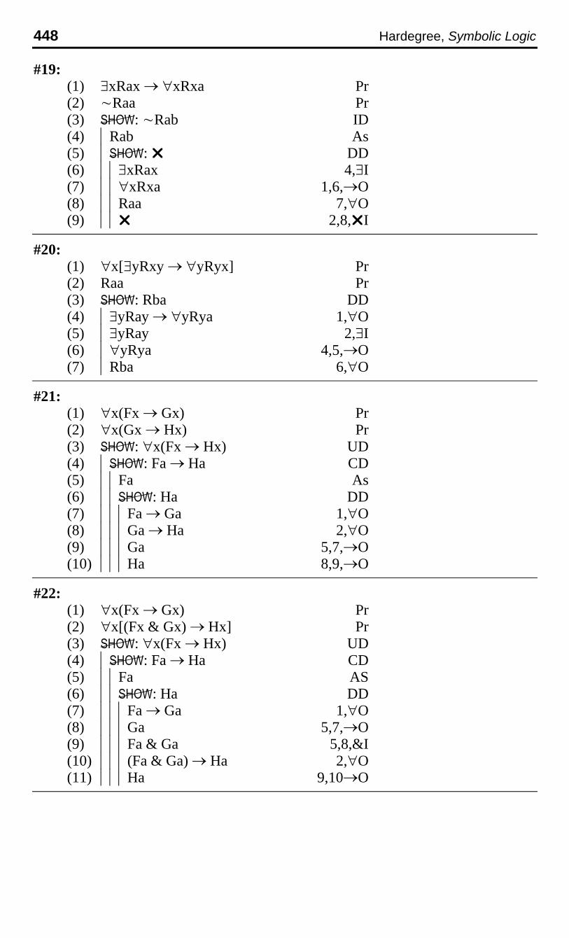
448 Hardegree, Symbolic Logic
#19:(1) ∃xRax → ∀xRxa Pr(2) ~Raa Pr(3) : ~Rab ID(4) |Rab As(5) |: ¸ DD(6) ||∃xRax 4,∃I(7) ||∀xRxa 1,6,→O(8) ||Raa 7,∀O(9) ||¸ 2,8,¸I
#20:(1) ∀x[∃yRxy → ∀yRyx] Pr(2) Raa Pr(3) : Rba DD(4) |∃yRay → ∀yRya 1,∀O(5) |∃yRay 2,∃I(6) |∀yRya 4,5,→O(7) |Rba 6,∀O
#21:(1) ∀x(Fx → Gx) Pr(2) ∀x(Gx → Hx) Pr(3) : ∀x(Fx → Hx) UD(4) |: Fa → Ha CD(5) ||Fa As(6) ||: Ha DD(7) |||Fa → Ga 1,∀O(8) |||Ga → Ha 2,∀O(9) |||Ga 5,7,→O(10) |||Ha 8,9,→O
#22:(1) ∀x(Fx → Gx) Pr(2) ∀x[(Fx & Gx) → Hx] Pr(3) : ∀x(Fx → Hx) UD(4) |: Fa → Ha CD(5) ||Fa AS(6) ||: Ha DD(7) |||Fa → Ga 1,∀O(8) |||Ga 5,7,→O(9) |||Fa & Ga 5,8,&I(10) |||(Fa & Ga) → Ha 2,∀O(11) |||Ha 9,10→O
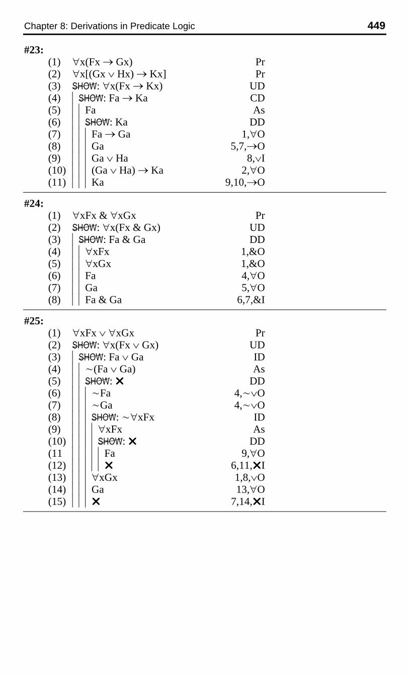
Chapter 8: Derivations in Predicate Logic 449
#23:(1) ∀x(Fx → Gx) Pr(2) ∀x[(Gx ∨ Hx) → Kx] Pr(3) : ∀x(Fx → Kx) UD(4) |: Fa → Ka CD(5) ||Fa As(6) ||: Ka DD(7) |||Fa → Ga 1,∀O(8) |||Ga 5,7,→O(9) |||Ga ∨ Ha 8,∨I(10) |||(Ga ∨ Ha) → Ka 2,∀O(11) |||Ka 9,10,→O
#24:(1) ∀xFx & ∀xGx Pr(2) : ∀x(Fx & Gx) UD(3) |: Fa & Ga DD(4) ||∀xFx 1,&O(5) ||∀xGx 1,&O(6) ||Fa 4,∀O(7) ||Ga 5,∀O(8) ||Fa & Ga 6,7,&I
#25:(1) ∀xFx ∨ ∀xGx Pr(2) : ∀x(Fx ∨ Gx) UD(3) |: Fa ∨ Ga ID(4) ||~(Fa ∨ Ga) As(5) ||: ¸ DD(6) |||~Fa 4,~∨O(7) |||~Ga 4,~∨O(8) |||: ~∀xFx ID(9) ||||∀xFx As(10) ||||: ¸ DD(11 |||||Fa 9,∀O(12) |||||¸ 6,11,¸I(13) |||∀xGx 1,8,∨O(14) |||Ga 13,∀O(15) |||¸ 7,14,¸I

450 Hardegree, Symbolic Logic
#26:(1) ~∃xFx Pr(2) : ∀x(Fx → Gx) UD(3) |: Fa → Ga CD(4) ||Fa As(5) ||: Ga ID(6) |||~Ga As(7) |||: ¸ DD(8) ||||∀x~Fx 1,~∃O(9) ||||~Fa 8,∀O(10) ||||¸ 4,9,¸I
#27:(1) ~∃x(Fx & Gx) Pr(2) : ∀x(Fx → ~Gx) UD(3) |: Fa → ~Ga CD(4) ||Fa As(5) ||: ~Ga ID(6) |||Ga As(7) |||: ¸ DD(8) ||||∀x~(Fx & Gx) 1,~∃O(9) ||||~(Fa & Ga) 8,∀O(10) ||||Fa & Ga 4,6,&I(11) ||||¸ 9,10,¸I
#28:(1) ∀x(Fx → Gx) Pr(2) ~∃x(Gx & Hx) Pr(3) : ∀x(Fx → ~Hx) UD(4) |: Fa → ~Ha CD(5) ||Fa As(6) ||: ~Ha ID(7) |||Ha As(8) |||: ¸ DD(9) ||||Fa → Ga 1,∀O(10) ||||Ga 5,9,→O(11) ||||Ga & Ha 7,10,&I(12) ||||∃x(Gx & Hx) 11,∃I(13) ||||¸ 2,12,¸I
#29:(1) ∀x(Fx → Gx) Pr(2) : ∀xFx → ∀xGx CD(3) |∀xFx As(4) |: ∀xGx UD(5) ||: Ga DD(6) |||Fa → Ga 1,∀O(7) |||Fa 3,∀O(8) |||Ga 6,7,→O
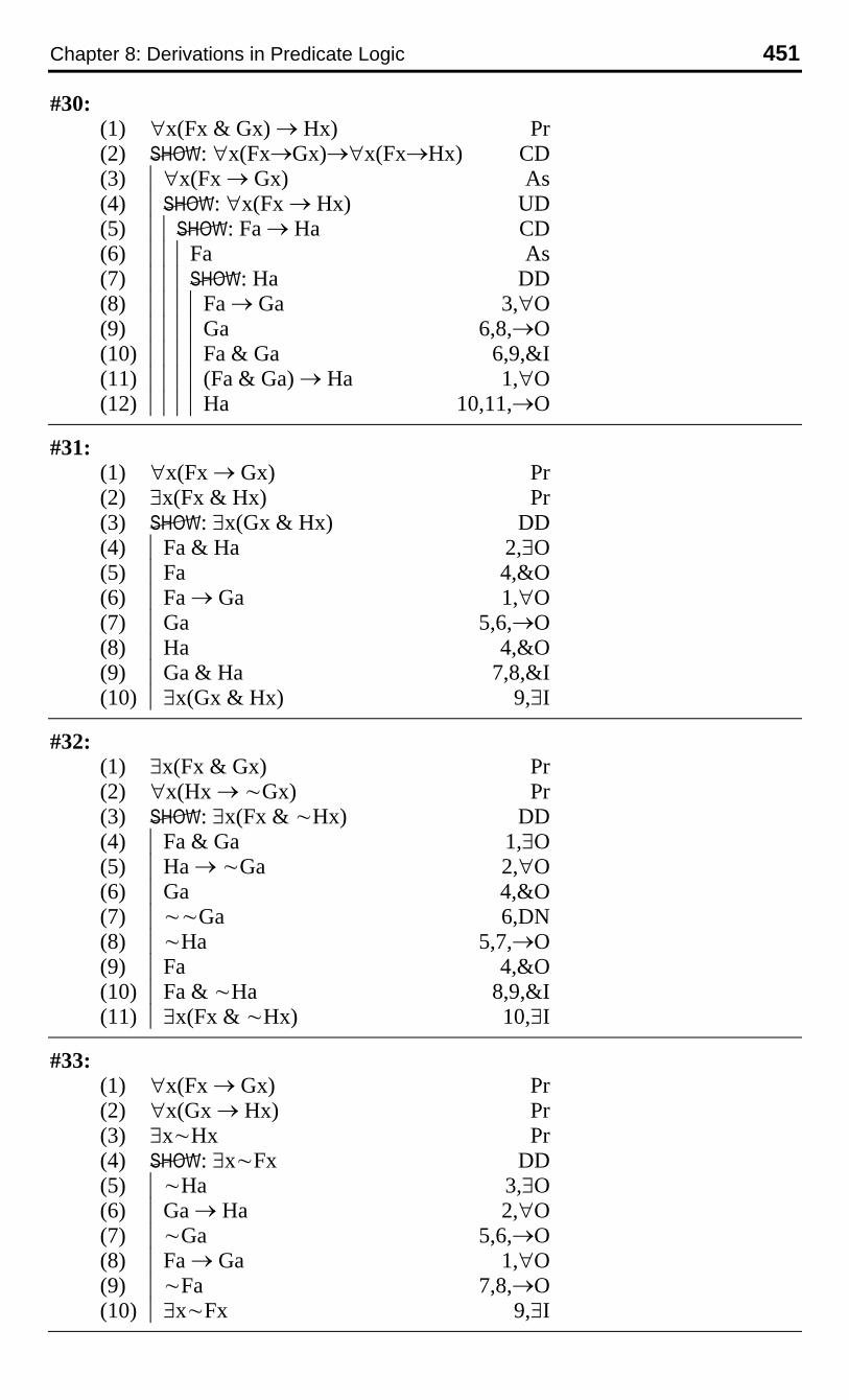
Chapter 8: Derivations in Predicate Logic 451
#30:(1) ∀x(Fx & Gx) → Hx) Pr(2) : ∀x(Fx→Gx)→∀x(Fx→Hx) CD(3) |∀x(Fx → Gx) As(4) |: ∀x(Fx → Hx) UD(5) ||: Fa → Ha CD(6) |||Fa As(7) |||: Ha DD(8) ||||Fa → Ga 3,∀O(9) ||||Ga 6,8,→O(10) ||||Fa & Ga 6,9,&I(11) ||||(Fa & Ga) → Ha 1,∀O(12) ||||Ha 10,11,→O
#31:(1) ∀x(Fx → Gx) Pr(2) ∃x(Fx & Hx) Pr(3) : ∃x(Gx & Hx) DD(4) |Fa & Ha 2,∃O(5) |Fa 4,&O(6) |Fa → Ga 1,∀O(7) |Ga 5,6,→O(8) |Ha 4,&O(9) |Ga & Ha 7,8,&I(10) |∃x(Gx & Hx) 9,∃I
#32:(1) ∃x(Fx & Gx) Pr(2) ∀x(Hx → ~Gx) Pr(3) : ∃x(Fx & ~Hx) DD(4) |Fa & Ga 1,∃O(5) |Ha → ~Ga 2,∀O(6) |Ga 4,&O(7) |~~Ga 6,DN(8) |~Ha 5,7,→O(9) |Fa 4,&O(10) |Fa & ~Ha 8,9,&I(11) |∃x(Fx & ~Hx) 10,∃I
#33:(1) ∀x(Fx → Gx) Pr(2) ∀x(Gx → Hx) Pr(3) ∃x~Hx Pr(4) : ∃x~Fx DD(5) |~Ha 3,∃O(6) |Ga → Ha 2,∀O(7) |~Ga 5,6,→O(8) |Fa → Ga 1,∀O(9) |~Fa 7,8,→O(10) |∃x~Fx 9,∃I
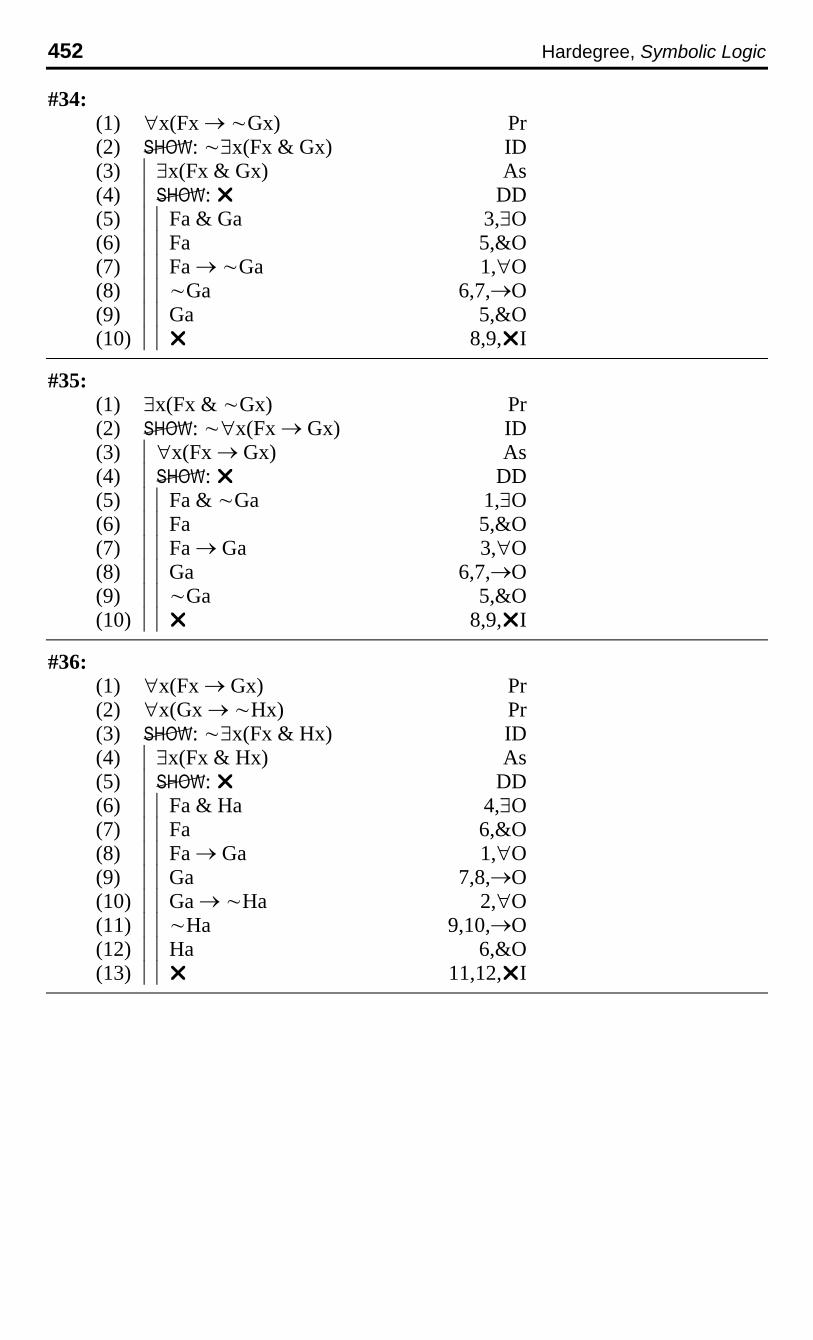
452 Hardegree, Symbolic Logic
#34:(1) ∀x(Fx → ~Gx) Pr(2) : ~∃x(Fx & Gx) ID(3) |∃x(Fx & Gx) As(4) |: ¸ DD(5) ||Fa & Ga 3,∃O(6) ||Fa 5,&O(7) ||Fa → ~Ga 1,∀O(8) ||~Ga 6,7,→O(9) ||Ga 5,&O(10) ||¸ 8,9,¸I
#35:(1) ∃x(Fx & ~Gx) Pr(2) : ~∀x(Fx → Gx) ID(3) |∀x(Fx → Gx) As(4) |: ¸ DD(5) ||Fa & ~Ga 1,∃O(6) ||Fa 5,&O(7) ||Fa → Ga 3,∀O(8) ||Ga 6,7,→O(9) ||~Ga 5,&O(10) ||¸ 8,9,¸I
#36:(1) ∀x(Fx → Gx) Pr(2) ∀x(Gx → ~Hx) Pr(3) : ~∃x(Fx & Hx) ID(4) |∃x(Fx & Hx) As(5) |: ¸ DD(6) ||Fa & Ha 4,∃O(7) ||Fa 6,&O(8) ||Fa → Ga 1,∀O(9) ||Ga 7,8,→O(10) ||Ga → ~Ha 2,∀O(11) ||~Ha 9,10,→O(12) ||Ha 6,&O(13) ||¸ 11,12,¸I
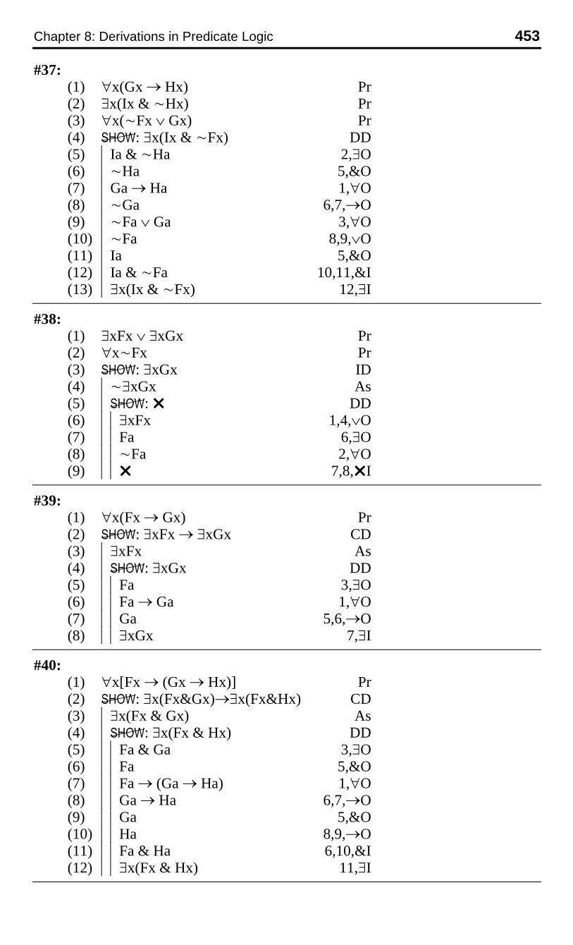
Chapter 8: Derivations in Predicate Logic 453
#37:(1) ∀x(Gx → Hx) Pr(2) ∃x(Ix & ~Hx) Pr(3) ∀x(~Fx ∨ Gx) Pr(4) : ∃x(Ix & ~Fx) DD(5) |Ia & ~Ha 2,∃O(6) |~Ha 5,&O(7) |Ga → Ha 1,∀O(8) |~Ga 6,7,→O(9) |~Fa ∨ Ga 3,∀O(10) |~Fa 8,9,∨O(11) |Ia 5,&O(12) |Ia & ~Fa 10,11,&I(13) |∃x(Ix & ~Fx) 12,∃I
#38:(1) ∃xFx ∨ ∃xGx Pr(2) ∀x~Fx Pr(3) : ∃xGx ID(4) |~∃xGx As(5) |: ¸ DD(6) ||∃xFx 1,4,∨O(7) ||Fa 6,∃O(8) ||~Fa 2,∀O(9) ||¸ 7,8,¸I
#39:(1) ∀x(Fx → Gx) Pr(2) : ∃xFx → ∃xGx CD(3) |∃xFx As(4) |: ∃xGx DD(5) ||Fa 3,∃O(6) ||Fa → Ga 1,∀O(7) ||Ga 5,6,→O(8) ||∃xGx 7,∃I
#40:(1) ∀x[Fx → (Gx → Hx)] Pr(2) : ∃x(Fx&Gx)→∃x(Fx&Hx) CD(3) |∃x(Fx & Gx) As(4) |: ∃x(Fx & Hx) DD(5) ||Fa & Ga 3,∃O(6) ||Fa 5,&O(7) ||Fa → (Ga → Ha) 1,∀O(8) ||Ga → Ha 6,7,→O(9) ||Ga 5,&O(10) ||Ha 8,9,→O(11) ||Fa & Ha 6,10,&I(12) ||∃x(Fx & Hx) 11,∃I

454 Hardegree, Symbolic Logic
#41:(1) ~∀x(Fx → Gx) Pr(2) : ∃x(Fx & ~Gx) ID(3) |~∃x(Fx & ~Gx) As(4) |: ¸ DD(5) ||∃x~(Fx → Gx) 1,~∀O(6) ||~(Fa → Ga) 5,∃O(7) ||Fa & ~Ga 6,~→O(8) ||∀x~(Fx & ~Gx) 3,~∃O(9) ||~(Fa & ~Ga) 8,∀O(10) ||¸ 7,9,¸I
#42:(1) ~∀xFx Pr(2) : ∃x(Fx → Gx) ID(3) |~∃x(Fx → Gx) As(4) |: ¸ DD(5) ||∃x~Fx 1,~∀O(6) ||~Fa 5,∃O(7) ||∀x~(Fx → Gx) 3,~∃O(8) ||~(Fa → Ga) 7,∀O(9) ||Fa & ~Ga 8,~→O(10) ||Fa 9,&O(11) ||¸ 6,10,¸I
#43:(1) ∀x(Gx → Hx) Pr(2) ∀x(Fx → Gx) Pr(3) : ~∀xHx → ∃x~Fx CD(4) |~∀xHx As(5) |: ∃x~Fx DD(6) ||∃x~Hx 4,~∀O(7) ||~Ha 6,∃O(8) ||Ga → Ha 1,∀O(9) ||~Ga 7,8,→O(10) ||Fa → Ga 2,∀O(11) ||~Fa 9,10,→O(12) ||∃x~Fx 11,∃I

Chapter 8: Derivations in Predicate Logic 455
#44:(1) ∃x(Fx ∨ Gx) Pr(2) : ∃xFx ∨ ∃xGx ID(3) |~(∃xFx ∨ ∃xGx) As(4) |: ¸ DD(5) ||~∃xFx 3,~∨O(6) ||~∃xGx 3,~∨O(7) ||Fa ∨ Ga 1,∃O(8) ||∀x~Fx 5,~∃O(9) ||~Fa 8,∀O(10) ||Ga 7,9,∨O(11) ||∀x~Gx 6,~∃O(12) ||~Ga 11,∀O(13) ||¸ 10,12,¸I
#45:(1) ∃x(Fx → Gx) Pr(2) : ∃x~Fx ∨ ∃xGx ID(3) |~(∃x~Fx ∨ ∃xGx) As(4) |: ¸ DD(5) ||~∃x~Fx 3,~∨O(6) ||~∃xGx 3,~∨O(7) ||Fa → Ga 1,∃O(8) ||∀x~~Fx 5,~∃O(9) ||~~Fa 8,∀O(10) ||Fa 9,DN(11) ||Ga 7,10,→O(12) ||∀x~Gx 6,~∃O(13) ||~Ga 12,∀O(14) ||¸ 11,13,¸I
#46:(1) ∃xFx → ∀xFx Pr(2) : ∀xFx ∨ ∀x~Fx ID(3) |~(∀xFx ∨ ∀x~Fx) As(4) |: ¸ DD(5) ||~∀xFx 3,~∨O(6) ||~∀x~Fx 3,~∨O(7) ||~∃xFx 1,5,→O(8) ||∀x~Fx 7,~∃O(9) ||¸ 6,8,¸I
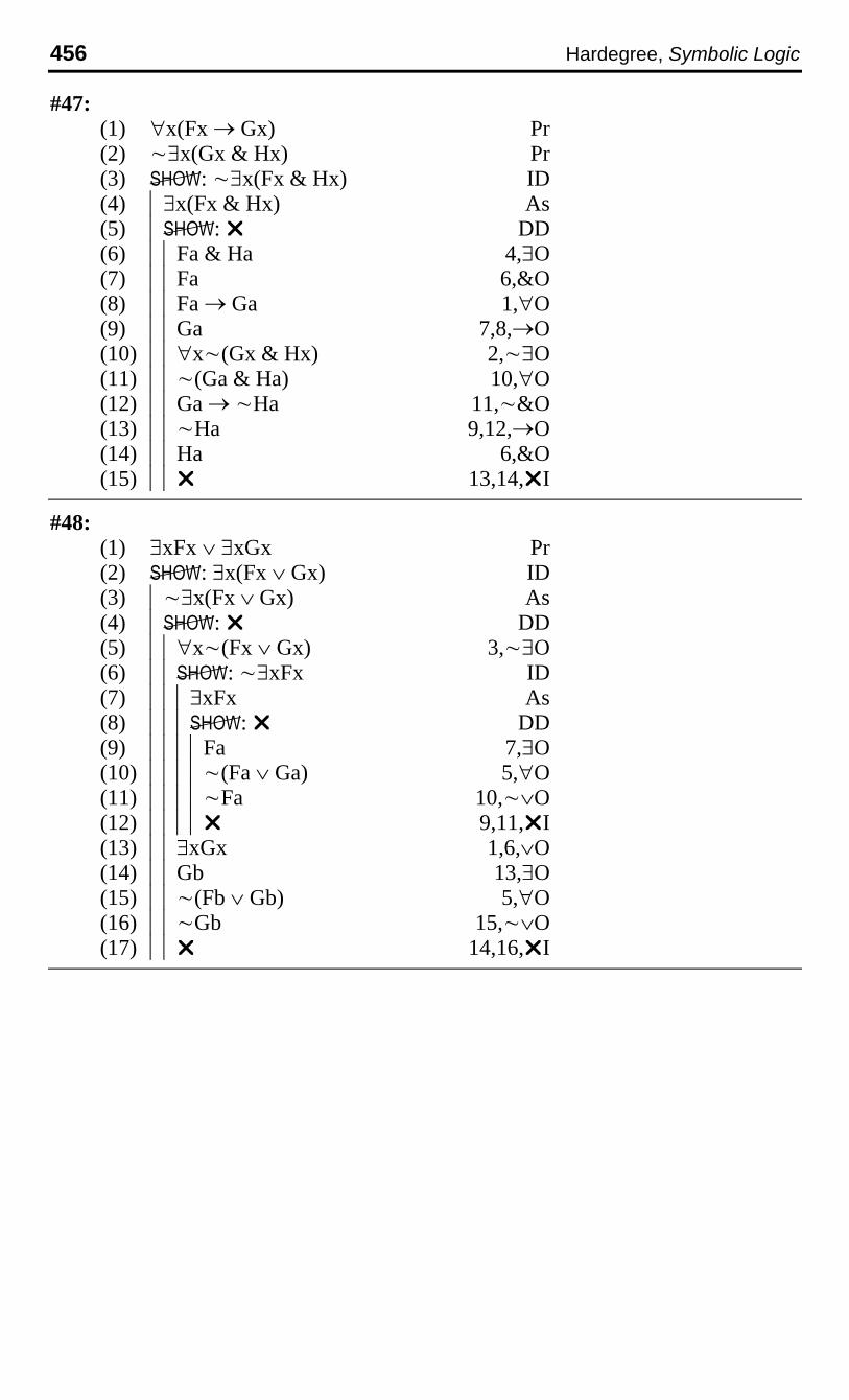
456 Hardegree, Symbolic Logic
#47:(1) ∀x(Fx → Gx) Pr(2) ~∃x(Gx & Hx) Pr(3) : ~∃x(Fx & Hx) ID(4) |∃x(Fx & Hx) As(5) |: ¸ DD(6) ||Fa & Ha 4,∃O(7) ||Fa 6,&O(8) ||Fa → Ga 1,∀O(9) ||Ga 7,8,→O(10) ||∀x~(Gx & Hx) 2,~∃O(11) ||~(Ga & Ha) 10,∀O(12) ||Ga → ~Ha 11,~&O(13) ||~Ha 9,12,→O(14) ||Ha 6,&O(15) ||¸ 13,14,¸I
#48:(1) ∃xFx ∨ ∃xGx Pr(2) : ∃x(Fx ∨ Gx) ID(3) |~∃x(Fx ∨ Gx) As(4) |: ¸ DD(5) ||∀x~(Fx ∨ Gx) 3,~∃O(6) ||: ~∃xFx ID(7) |||∃xFx As(8) |||: ¸ DD(9) ||||Fa 7,∃O(10) ||||~(Fa ∨ Ga) 5,∀O(11) ||||~Fa 10,~∨O(12) ||||¸ 9,11,¸I(13) ||∃xGx 1,6,∨O(14) ||Gb 13,∃O(15) ||~(Fb ∨ Gb) 5,∀O(16) ||~Gb 15,~∨O(17) ||¸ 14,16,¸I
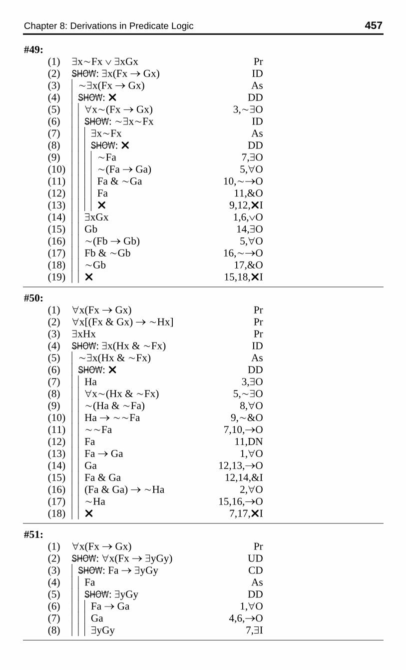
Chapter 8: Derivations in Predicate Logic 457
#49:(1) ∃x~Fx ∨ ∃xGx Pr(2) : ∃x(Fx → Gx) ID(3) |~∃x(Fx → Gx) As(4) |: ¸ DD(5) ||∀x~(Fx → Gx) 3,~∃O(6) ||: ~∃x~Fx ID(7) |||∃x~Fx As(8) |||: ¸ DD(9) ||||~Fa 7,∃O(10) ||||~(Fa → Ga) 5,∀O(11) ||||Fa & ~Ga 10,~→O(12) ||||Fa 11,&O(13) ||||¸ 9,12,¸I(14) ||∃xGx 1,6,∨O(15) ||Gb 14,∃O(16) ||~(Fb → Gb) 5,∀O(17) ||Fb & ~Gb 16,~→O(18) ||~Gb 17,&O(19) ||¸ 15,18,¸I
#50:(1) ∀x(Fx → Gx) Pr(2) ∀x[(Fx & Gx) → ~Hx] Pr(3) ∃xHx Pr(4) : ∃x(Hx & ~Fx) ID(5) |~∃x(Hx & ~Fx) As(6) |: ¸ DD(7) ||Ha 3,∃O(8) ||∀x~(Hx & ~Fx) 5,~∃O(9) ||~(Ha & ~Fa) 8,∀O(10) ||Ha → ~~Fa 9,~&O(11) ||~~Fa 7,10,→O(12) ||Fa 11,DN(13) ||Fa → Ga 1,∀O(14) ||Ga 12,13,→O(15) ||Fa & Ga 12,14,&I(16) ||(Fa & Ga) → ~Ha 2,∀O(17) ||~Ha 15,16,→O(18) ||¸ 7,17,¸I
#51:(1) ∀x(Fx → Gx) Pr(2) : ∀x(Fx → ∃yGy) UD(3) |: Fa → ∃yGy CD(4) ||Fa As(5) ||: ∃yGy DD(6) |||Fa → Ga 1,∀O(7) |||Ga 4,6,→O(8) |||∃yGy 7,∃I
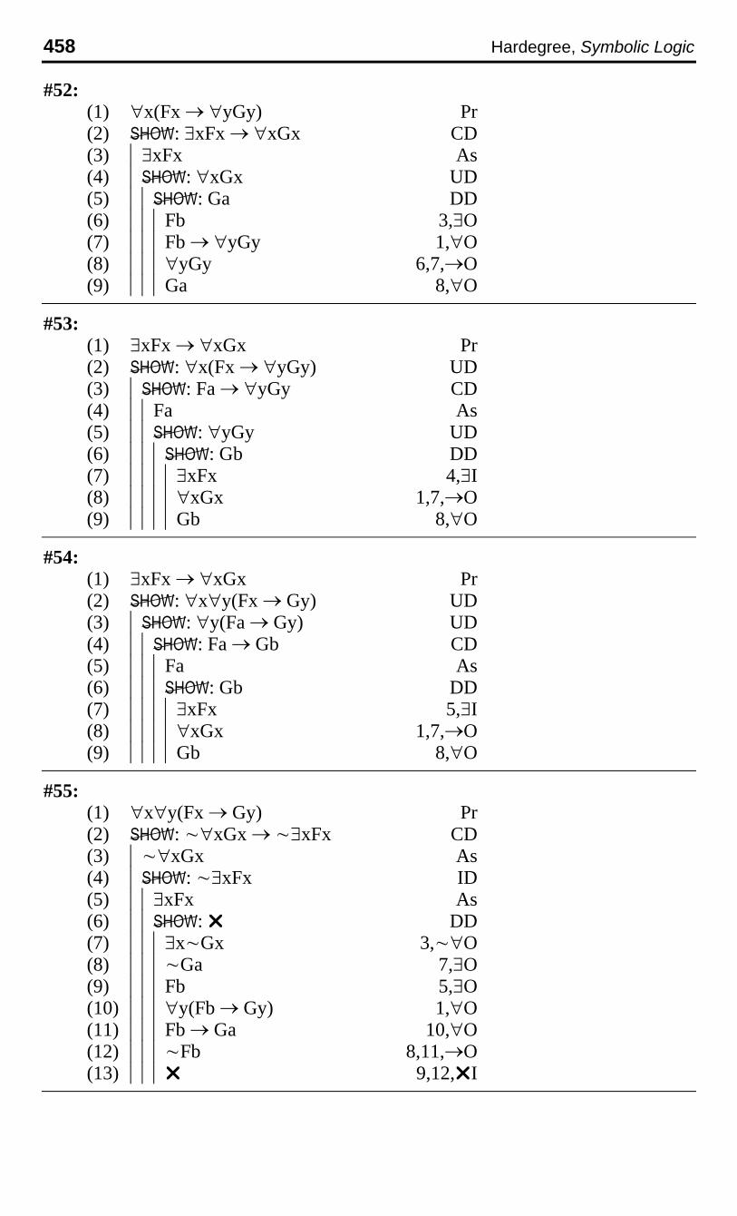
458 Hardegree, Symbolic Logic
#52:(1) ∀x(Fx → ∀yGy) Pr(2) : ∃xFx → ∀xGx CD(3) |∃xFx As(4) |: ∀xGx UD(5) ||: Ga DD(6) |||Fb 3,∃O(7) |||Fb → ∀yGy 1,∀O(8) |||∀yGy 6,7,→O(9) |||Ga 8,∀O
#53:(1) ∃xFx → ∀xGx Pr(2) : ∀x(Fx → ∀yGy) UD(3) |: Fa → ∀yGy CD(4) ||Fa As(5) ||: ∀yGy UD(6) |||: Gb DD(7) ||||∃xFx 4,∃I(8) ||||∀xGx 1,7,→O(9) ||||Gb 8,∀O
#54:(1) ∃xFx → ∀xGx Pr(2) : ∀x∀y(Fx → Gy) UD(3) |: ∀y(Fa → Gy) UD(4) ||: Fa → Gb CD(5) |||Fa As(6) |||: Gb DD(7) ||||∃xFx 5,∃I(8) ||||∀xGx 1,7,→O(9) ||||Gb 8,∀O
#55:(1) ∀x∀y(Fx → Gy) Pr(2) : ~∀xGx → ~∃xFx CD(3) |~∀xGx As(4) |: ~∃xFx ID(5) ||∃xFx As(6) ||: ¸ DD(7) |||∃x~Gx 3,~∀O(8) |||~Ga 7,∃O(9) |||Fb 5,∃O(10) |||∀y(Fb → Gy) 1,∀O(11) |||Fb → Ga 10,∀O(12) |||~Fb 8,11,→O(13) |||¸ 9,12,¸I

Chapter 8: Derivations in Predicate Logic 459
#56:(1) ∃xFx → ∃x~Gx Pr(2) : ∀x(Fx → ~∀yGy) UD(3) |: Fa → ~∀yGy CD(4) ||Fa As(5) ||: ~∀yGy ID(6) |||∀yGy As(7) |||: ¸ DD(8) ||||∃xFx 4,∃I(9) ||||∃x~Gx 1,8,→O(10) ||||~Gb 9,∃O(11) ||||Gb 6,∀O(12) ||||¸ 10,11,¸I
#57:(1) ∃xFx → ∀x~Gx Pr(2) : ∀x(Fx → ~∃yGy) UD(3) |: Fa → ~∃yGy CD(4) ||Fa As(5) ||: ~∃yGy ID(6) |||∃yGy As(7) |||: ¸ DD(8) ||||∃xFx 4,∃I(9) ||||∀x~Gx 1,8,→O(10) ||||Gb 6,∃O(11) ||||~Gb 9,∀O(12) ||||¸ 10,11,¸I
#58:(1) ∀x(Fx → ~∃yGy) Pr(2) : ∃xFx → ∀x~Gx CD(3) |∃xFx As(4) |: ∀x~Gx UD(5) ||: ~Ga ID(6) |||Ga As(7) |||: ¸ DD(8) ||||Fb 3,∃O(9) ||||Fb → ~∃yGy 1,∀O(10) ||||~∃yGy 8,9,→O(11) ||||∀y~Gy 10,~∃O(12) ||||~Ga 11,∀O(13) ||||¸ 6,12,¸I

460 Hardegree, Symbolic Logic
#59:(1) ∀x(∃yFy → Gx) Pr(2) : ∀x∀y(Fx → Gy) UD(3) |: ∀y(Fa → Gy) UD(4) ||: Fa → Gb CD(5) |||Fa As(6) |||: Gb DD(7) ||||∃yFy → Gb 1,∀O(8) ||||∃yFy 5,∃I(9) ||||Gb 7,8,→O
#60:(1) ∃xFx → ∀xFx Pr(2) : ∀x∀y(Fx ↔ Fy) UD(3) |: ∀y(Fa ↔ Fy) UD(4) ||: Fa ↔ Fb DD(5) |||: Fa → Fb CD(6) ||||Fa As(7) ||||: Fb DD(8) |||||∃xFx 6,∃I(9) |||||∀xFx 1,8,→O(10) |||||Fb 9,∀O(11) |||: Fb → Fa CD(12) ||||Fb As(13) ||||: Fa DD(14) |||||∃xFx 12,∃I(15) |||||∀xFx 1,14,→O(16) |||||Fa 15,∀O(17) |||Fa ↔ Fb 5,11,↔I
#61:(1) ∀x∀yRxy Pr(2) : ∀x∀yRyx UD(3) |: ∀yRya UD(4) ||: Rba DD(5) |||∀yRby 1,∀O(6) |||Rba 5,∀O
#62:(1) ∃xRxx Pr(2) : ∃x∃yRxy DD(3) |Raa 1,∃O(4) |∃yRay 3,∃I(5) |∃x∃yRxy 4,∃I
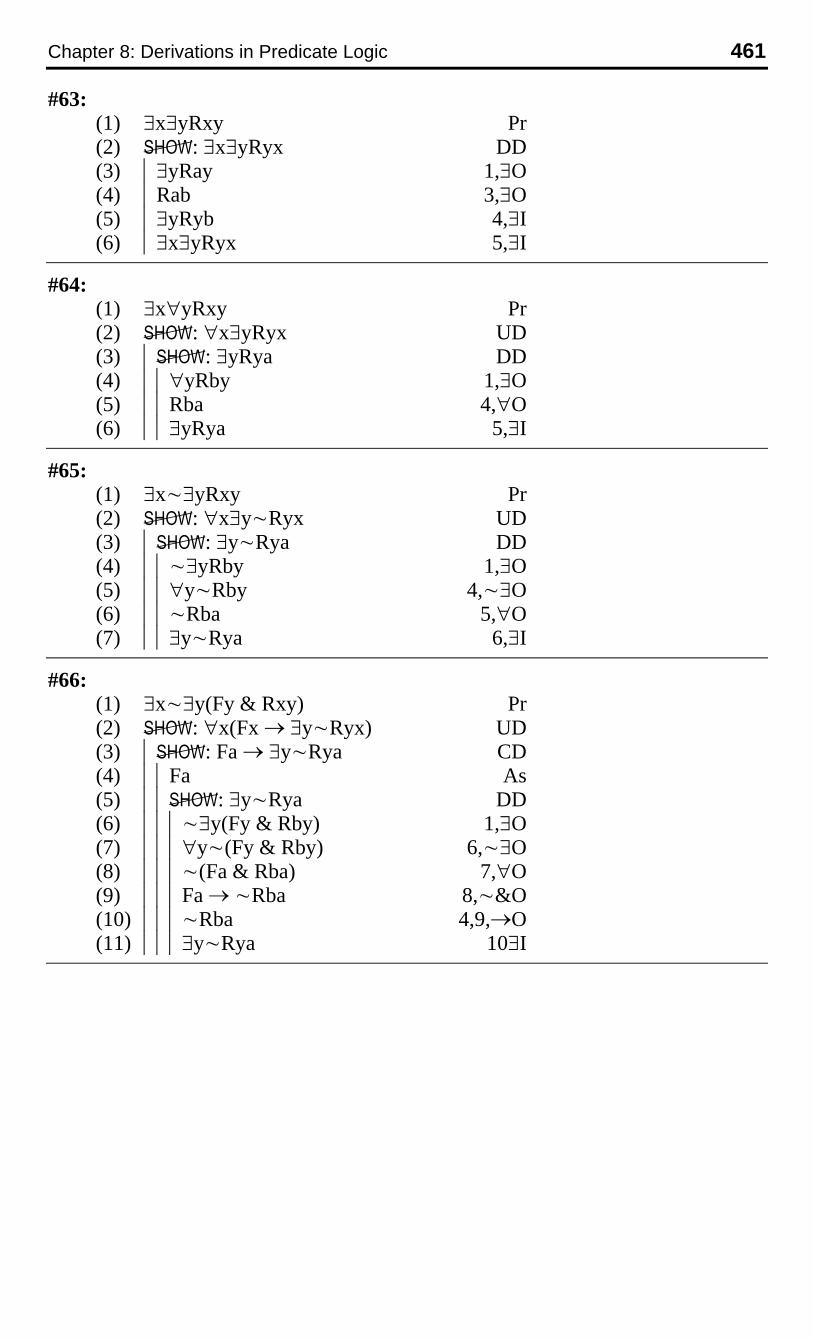
Chapter 8: Derivations in Predicate Logic 461
#63:(1) ∃x∃yRxy Pr(2) : ∃x∃yRyx DD(3) |∃yRay 1,∃O(4) |Rab 3,∃O(5) |∃yRyb 4,∃I(6) |∃x∃yRyx 5,∃I
#64:(1) ∃x∀yRxy Pr(2) : ∀x∃yRyx UD(3) |: ∃yRya DD(4) ||∀yRby 1,∃O(5) ||Rba 4,∀O(6) ||∃yRya 5,∃I
#65:(1) ∃x~∃yRxy Pr(2) : ∀x∃y~Ryx UD(3) |: ∃y~Rya DD(4) ||~∃yRby 1,∃O(5) ||∀y~Rby 4,~∃O(6) ||~Rba 5,∀O(7) ||∃y~Rya 6,∃I
#66:(1) ∃x~∃y(Fy & Rxy) Pr(2) : ∀x(Fx → ∃y~Ryx) UD(3) |: Fa → ∃y~Rya CD(4) ||Fa As(5) ||: ∃y~Rya DD(6) |||~∃y(Fy & Rby) 1,∃O(7) |||∀y~(Fy & Rby) 6,~∃O(8) |||~(Fa & Rba) 7,∀O(9) |||Fa → ~Rba 8,~&O(10) |||~Rba 4,9,→O(11) |||∃y~Rya 10∃I

462 Hardegree, Symbolic Logic
#67:(1) ∀x(Fx → ∃y~Kxy) Pr(2) ∃x(Gx & ∀yKxy) Pr(3) : ∃x(Gx & ~Fx) ID(4) |~∃x(Gx & ~Fx) As(5) |: ¸ DD(6) ||∀x~(Gx & ~Fx) 4,~∃O(7) ||Ga & ∀yKay 2,∃O(8) ||Ga 7,&O(9) ||~(Ga & ~Fa) 6,∀O(10) ||Ga → ~~Fa 9,~&O(11) ||~~Fa 8,10,→O(12) ||Fa 11,DN(13) ||Fa → ∃y~Kay 1,∀O(14) ||∃y~Kay 12,13,→O(15) ||~Kab 14,∃O(16) ||∀yKay 7,&O(17) ||Kab 16,∀O(18) ||¸ 15,17,¸I
#68:(1) ∃x[Fx & ~∃y(Gy & Rxy)] Pr(2) : ∀x[Gx → ∃y(Fy & ~Ryx)] UD(3) |: Ga → ∃y(Fy & ~Rya) CD(4) ||Ga As(5) ||: ∃y(Fy & ~Rya) DD(6) |||Fb & ~∃y(Gy & Rby) 1,∃O(7) |||Fb 6,&O(8) |||~∃y(Gy & Rby) 6,&O(9) |||∀y~(Gy & Rby) 8,~∃O(10) |||~(Ga & Rba) 9,∀O(11) |||Ga → ~Rba 10,~&O(12) |||~Rba 4,11,→O(13) |||Fb & ~Rba 7,12,&I(14) |||∃y(Fy & ~Rya) 13,∃I
#69:(1) ∃x[Fx & ∀y(Gy → Rxy)] Pr(2) : ∀x[Gx → ∃y(Fy & Ryx)] UD(3) |: Ga → ∃y(Fy & Rya) CD(4) ||Ga As(5) ||: ∃y(Fy & Rya) DD(6) |||Fb & ∀y(Gy → Rby) 1,∃O(7) |||∀y(Gy → Rby) 6,&O(8) |||Ga → Rba 7,∀O(9) |||Rba 4,8,→O(10) |||Fb 6,&O(11) |||Fb & Rba 9,10,&I(12) |||∃y(Fy & Rya) 11,∃I
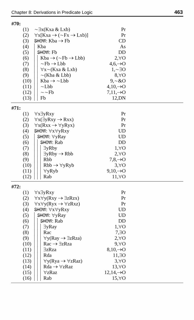
Chapter 8: Derivations in Predicate Logic 463
#70:(1) ~∃x(Kxa & Lxb) Pr(2) ∀x[Kxa → (~Fx → Lxb)] Pr(3) : Kba → Fb CD(4) |Kba As(5) |: Fb DD(6) ||Kba → (~Fb → Lbb) 2,∀O(7) ||~Fb → Lbb 4,6,→O(8) ||∀x~(Kxa & Lxb) 1,~∃O(9) ||~(Kba & Lbb) 8,∀O(10) ||Kba → ~Lbb 9,~&O(11) ||~Lbb 4,10,→O(12) ||~~Fb 7,11,→O(13) ||Fb 12,DN
#71:(1) ∀x∃yRxy Pr(2) ∀x(∃yRxy → Rxx) Pr(3) ∀x(Rxx → ∀yRyx) Pr(4) : ∀x∀yRxy UD(5) |: ∀yRay UD(6) ||: Rab DD(7) |||∃yRby 1,∀O(8) |||∃yRby → Rbb 2,∀O(9) |||Rbb 7,8,→O(10) |||Rbb → ∀yRyb 3,∀O(11) |||∀yRyb 9,10,→O(12) |||Rab 11,∀O
#72:(1) ∀x∃yRxy Pr(2) ∀x∀y(Rxy → ∃zRzx) Pr(3) ∀x∀y(Ryx → ∀zRxz) Pr(4) : ∀x∀yRxy UD(5) |: ∀yRay UD(6) ||: Rab DD(7) |||∃yRay 1,∀O(8) |||Rac 7,∃O(9) |||∀y(Ray → ∃zRza) 2,∀O(10) |||Rac → ∃zRza 9,∀O(11) |||∃zRza 8,10,→O(12) |||Rda 11,∃O(13) |||∀y(Rya → ∀zRaz) 3,∀O(14) |||Rda → ∀zRaz 13,∀O(15) |||∀zRaz 12,14,→O(16) |||Rab 15,∀O
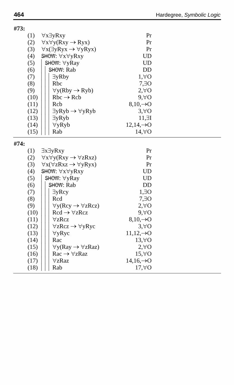
464 Hardegree, Symbolic Logic
#73:(1) ∀x∃yRxy Pr(2) ∀x∀y(Rxy → Ryx) Pr(3) ∀x(∃yRyx → ∀yRyx) Pr(4) : ∀x∀yRxy UD(5) |: ∀yRay UD(6) ||: Rab DD(7) |||∃yRby 1,∀O(8) |||Rbc 7,∃O(9) |||∀y(Rby → Ryb) 2,∀O(10) |||Rbc → Rcb 9,∀O(11) |||Rcb 8,10,→O(12) |||∃yRyb → ∀yRyb 3,∀O(13) |||∃yRyb 11,∃I(14) |||∀yRyb 12,14,→O(15) |||Rab 14,∀O
#74:(1) ∃x∃yRxy Pr(2) ∀x∀y(Rxy → ∀zRxz) Pr(3) ∀x(∀zRxz → ∀yRyx) Pr(4) : ∀x∀yRxy UD(5) |: ∀yRay UD(6) ||: Rab DD(7) |||∃yRcy 1,∃O(8) |||Rcd 7,∃O(9) |||∀y(Rcy → ∀zRcz) 2,∀O(10) |||Rcd → ∀zRcz 9,∀O(11) |||∀zRcz 8,10,→O(12) |||∀zRcz → ∀yRyc 3,∀O(13) |||∀yRyc 11,12,→O(14) |||Rac 13,∀O(15) |||∀y(Ray → ∀zRaz) 2,∀O(16) |||Rac → ∀zRaz 15,∀O(17) |||∀zRaz 14,16,→O(18) |||Rab 17,∀O
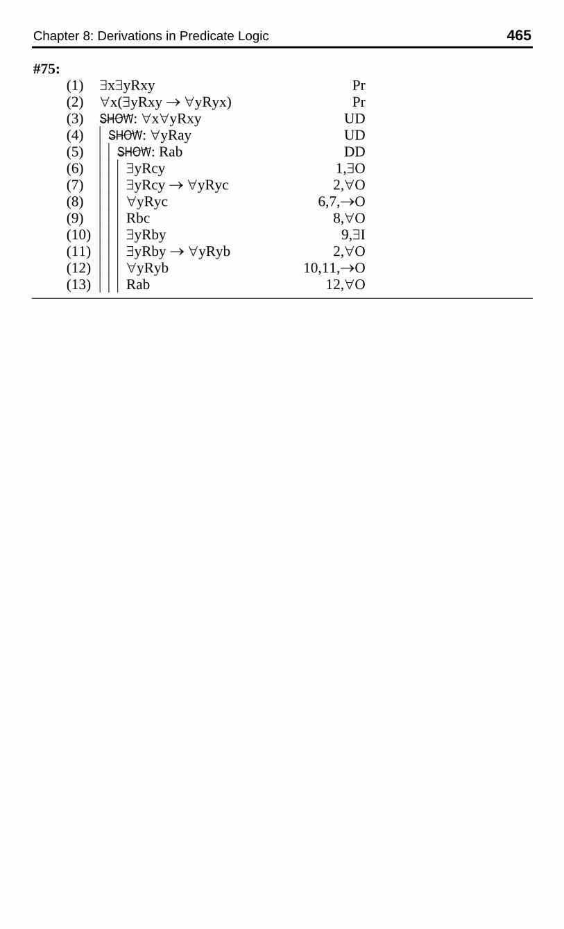
Chapter 8: Derivations in Predicate Logic 465
#75:(1) ∃x∃yRxy Pr(2) ∀x(∃yRxy → ∀yRyx) Pr(3) : ∀x∀yRxy UD(4) |: ∀yRay UD(5) ||: Rab DD(6) |||∃yRcy 1,∃O(7) |||∃yRcy → ∀yRyc 2,∀O(8) |||∀yRyc 6,7,→O(9) |||Rbc 8,∀O(10) |||∃yRby 9,∃I(11) |||∃yRby → ∀yRyb 2,∀O(12) |||∀yRyb 10,11,→O(13) |||Rab 12,∀O

466 Hardegree, Symbolic Logic
#76:(1) ∀x[Kxa → ∀y(Kyb → Rxy)] Pr(2) ∀x(Fx → Kxb) Pr(3) ∃x[Kxa & ∃y(Fy & ~Rxy)] Pr(4) : ∃xGx ID(5) |~∃xGx As(6) |: ¸ DD(7) ||Kca & ∃y(Fy & ~Rcy) 3,∃O(8) ||∃y(Fy & ~Rcy) 7,&O(9) ||Fd & ~Rcd 8,∃O(10) ||Fd 9,&O(11) ||Kca → ∀y(Kyb → Rcy) 1,∀O(12) ||Kca 7,&O(13) ||∀y(Kyb → Rcy) 11,12,→O(14) ||Kdb → Rcd 13,∀O(15) ||Fd → Kdb 2,∀O(16) ||Kdb 10,15,→O(17) ||Rcd 14,16,→O(18) ||~Rcd 9,&O(19) ||¸ 17,18,¸I
#77:(1) ∃xFx Pr(2) ∀x[Fx → ∃y(Fy & Ryx)] Pr(3) ∀x∀y(Rxy → Ryx) Pr(4) : ∃x∃y(Rxy & Ryx) DD(5) |Fa 1,∃O(6) |Fa → ∃y(Fy & Rya) 2,∀O(7) |∃y(Fy & Rya) 5,6,→O(8) |Fb & Rba 7,∃O(9) |Rba 8,&O(10) |∀y(Rby → Ryb) 3,∀O(11) |Rba → Rab 10,∀O(12) |Rab 9,11,→O(13) |Rab & Rba 9,12,&I(14) |∃y(Ray & Rya) 13,∃I(15) |∃x∃y(Rxy & Ryx) 14,∃I

Chapter 8: Derivations in Predicate Logic 467
#78:(1) ∃x(Fx & Kxa) Pr(2) ∃x[Fx & ∀y(Kya → ~Rxy)] Pr(3) : ∃x[Fx & ∃y(Fy & ~Ryx)] DD(4) |Fb & Kba 1,∃O(5) |Fc & ∀y(Kya → ~Rcy) 2,∃O(6) |∀y(Kya → ~Rcy) 5,&O(7) |Kba → ~Rcb 6,∀O(8) |Kba 4,&O(9) |~Rcb 7,8,→O(10) |Fc 5,&O(11) |Fc & ~Rcb 9,10,&I(12) |∃y(Fy & ~Ryb) 11,∃I(13) |Fb 4,&O(14) |Fb & ∃y(Fy & ~Ryb) 12,13,&I(15) |∃x[Fx & ∃y(Fy & ~Ryx)] 14,∃I
#79:(1) ∃x[Fx & ∀y(Gy → Rxy)] Pr(2) ~∃x[Fx & ∃y(Hy & Rxy)] Pr(3) : ~∃x(Gx & Hx) ID(4) |∃x(Gx & Hx) As(5) |: ¸ DD(6) ||Fa & ∀y(Gy → Ray) 1,∃O(7) ||∀x~[Fx & ∃y(Hy & Rxy)] 2,~∃O(8) ||~[Fa & ∃y(Hy & Ray)] 7,∀O(9) ||Fa → ~∃y(Hy & Ray) 8,~&O(10) ||Fa 6,&O(11) ||~∃y(Hy & Ray) 9,10,→O(12) ||∀y~(Hy & Ray) 11,~∃O(13) ||Gb & Hb 4,∃O(14) ||~(Hb & Rab) 12,∀O(15) ||Hb → ~Rab 14,~&O(16) ||Hb 13,&O(17) ||~Rab 15,16,→O(18) ||∀y(Gy → Ray) 6,&O(19) ||Gb → Rab 18,∀O(20) ||Gb 13,&O(21) ||Rab 19,20,→O(22) ||¸ 17,21,¸I
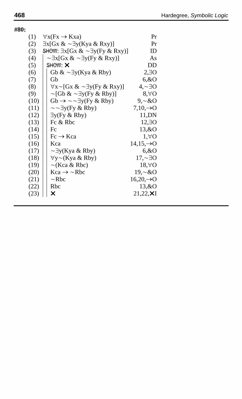
468 Hardegree, Symbolic Logic
#80:(1) ∀x(Fx → Kxa) Pr(2) ∃x[Gx & ~∃y(Kya & Rxy)] Pr(3) : ∃x[Gx & ~∃y(Fy & Rxy)] ID(4) |~∃x[Gx & ~∃y(Fy & Rxy)] As(5) |: ¸ DD(6) ||Gb & ~∃y(Kya & Rby) 2,∃O(7) ||Gb 6,&O(8) ||∀x~[Gx & ~∃y(Fy & Rxy)] 4,~∃O(9) ||~[Gb & ~∃y(Fy & Rby)] 8,∀O(10) ||Gb → ~~∃y(Fy & Rby) 9,~&O(11) ||~~∃y(Fy & Rby) 7,10,→O(12) ||∃y(Fy & Rby) 11,DN(13) ||Fc & Rbc 12,∃O(14) ||Fc 13,&O(15) ||Fc → Kca 1,∀O(16) ||Kca 14,15,→O(17) ||~∃y(Kya & Rby) 6,&O(18) ||∀y~(Kya & Rby) 17,~∃O(19) ||~(Kca & Rbc) 18,∀O(20) ||Kca → ~Rbc 19,~&O(21) ||~Rbc 16,20,→O(22) ||Rbc 13,&O(23) ||¸ 21,22,¸I