Chapter 7 Physical Layer and Transmission Media...7.1.2 Transmission Impairment Signals travel through transmission media, which are not perfect. The imperfection causes signal impairment

Copyright © The McGraw-Hill Companies, Inc. Permission required for reproduction or display.7.1

.

Chapter 7

Physical Layer

and

Transmission

Media


Chapter 7: Outline

7.1 DATA AND SIGNAL

7.2 DIGITAL TRANSMISSION

7.3ANALOG TRANSMISSION

7.4 BANDWIDTH UTILIZATION

7.5TRANSMISSION MEDIA


Chapter 7: Objective

We first discuss the relationship between data and signals. We

then show how data and signals can be both analog and digital.

We then concentrate on digital transmission. We show how to

convert digital and analog data to digital signals.

Next, we concentrate on analog transmission. We show how to

convert digital and analog data to analog signals.

We then talk about multiplexing techniques and how they can

combine several channels.

Finally, we go below the physical layer and discuss the

transmission media.


7-1 DATA AND SIGNALS

At the physical layer, the communication isnode-to-node, but the nodes exchangeelectromagnetic signals. Figure 7.1 uses thesame scenario we showed in four earlierchapters, but the communication is now atthe physical layer.


Figure 7.1: Communication at the physical layer


7.1.1 Analog and Digital

Data can be analog or digital. The term analog data

refers to information that is continuous. Digital data

take on discrete values.

Like the data they represent, signals can be either

analog or digital. An analog signal has infinitely

many levels of intensity over a period of time. A

digital signal, on the other hand, can have only a

limited number of defined values. Although each

value can be any number, it is often as simple as 1

and 0.


7.1.1 (continued)

Analog Signals

Time and Frequency Domains

Composite Signals

Bandwidth

Digital Signals

Bit Rate

Bit Length

Digital Signal as a Composite Analog Signal

Transmission of Digital Signals

Baseband Transmission

Broadband Transmission


Figure 7.2: Comparison of analog and digital signals


Figure 7.3: A sine wave


Figure 7.4: Wavelength and period


Figure 7.5: The time-domain and frequency-domain plots of a sine wave


12

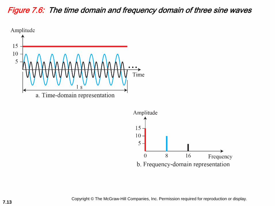
The frequency domain is more compact and useful when we

are dealing with more than one sine wave. For example,

Figure 7.6 shows three sine waves, each with different

amplitude and frequency. All can be represented by three

spikes in the frequency domain.

Example 7.1


Figure 7.6: The time domain and frequency domain of three sine waves


Figure 7.7: The bandwidth of periodic and nonperiodic composite signals


Figure 7.8: Two digital signals: one with two signal levels and the other with four signal levels


Assume we need to download text documents at the rate of

100 pages per minute. What is the required bit rate of the

channel? A page is an average of 24 lines with 80 characters

in each line. If we assume that one character requires 8 bits,

the bit rate is

Example 7.2


Figure 7.9: The time and frequency domains of periodic and nonperiodic digital signals


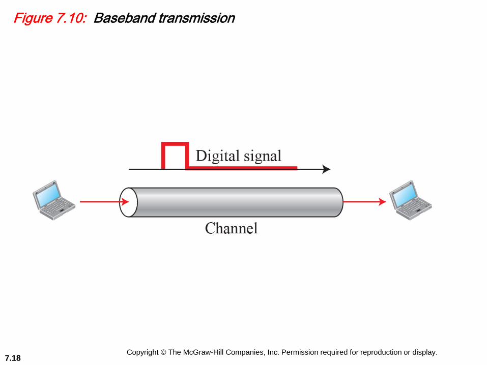
Figure 7.10: Baseband transmission


An example of a dedicated channel where the entire

bandwidth of the medium is used as one single channel is a

LAN. Almost every wired LAN today uses a dedicated

channel for two stations communicating with each other.

Example 7.3


Figure 7.11: Bandwidth of a band-pass channel


Figure 7.12: Modulation of a digital signal for transmission on a band-pass channel


An example of broadband transmission using modulation is

the sending of computer data through a telephone subscriber

line, the line connecting a resident to the central telephone

office. Although this channel can be used as a low-pass

channel, it is normally considered a band-pass channel. One

reason is that the bandwidth is so narrow (4 kHz) that if we

treat the channel as low-pass and use it for baseband

transmission, the maximum bit rate can be only 8 kbps

(explained later). The solution is to consider the channel a

band-pass channel, convert the digital signal from the

computer to an analog signal, and send the analog signal.

Example 7.4


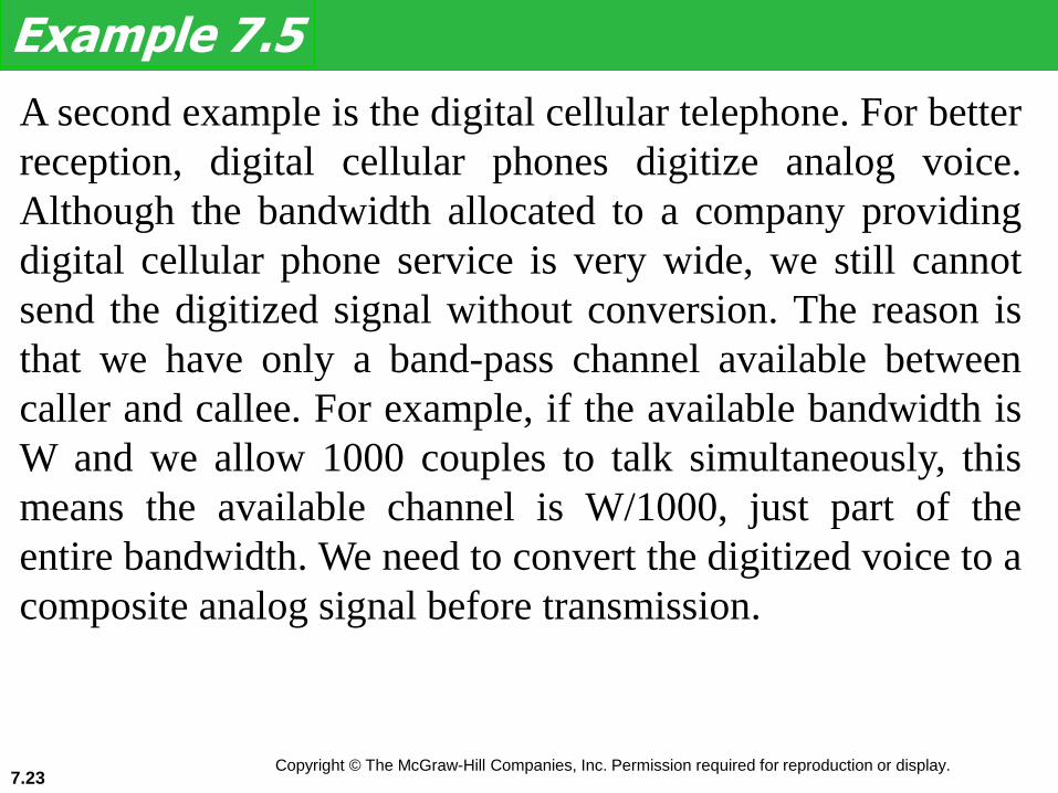
A second example is the digital cellular telephone. For better

reception, digital cellular phones digitize analog voice.

Although the bandwidth allocated to a company providing

digital cellular phone service is very wide, we still cannot

send the digitized signal without conversion. The reason is

that we have only a band-pass channel available between

caller and callee. For example, if the available bandwidth is

W and we allow 1000 couples to talk simultaneously, this

means the available channel is W/1000, just part of the

entire bandwidth. We need to convert the digitized voice to a

composite analog signal before transmission.

Example 7.5


7.1.2 Transmission Impairment

Signals travel through transmission media, which

are not perfect. The imperfection causes signal

impairment. This means that the signal at the

beginning of the medium is not the same as the

signal at the end of the medium. What is sent is not

what is received. Three causes of impairment are

attenuation, distortion, and noise.


7.1.2 (continued)

Attenuation

Distortion

Signal-to-Noise Ratio (SNR)

Noise


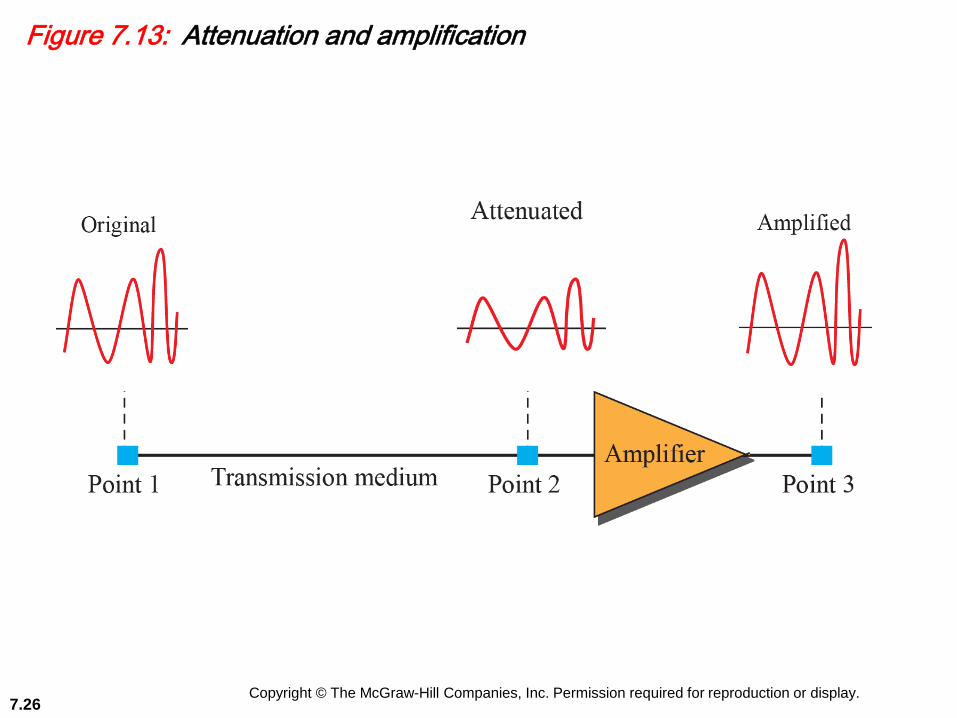
Figure 7.13: Attenuation and amplification


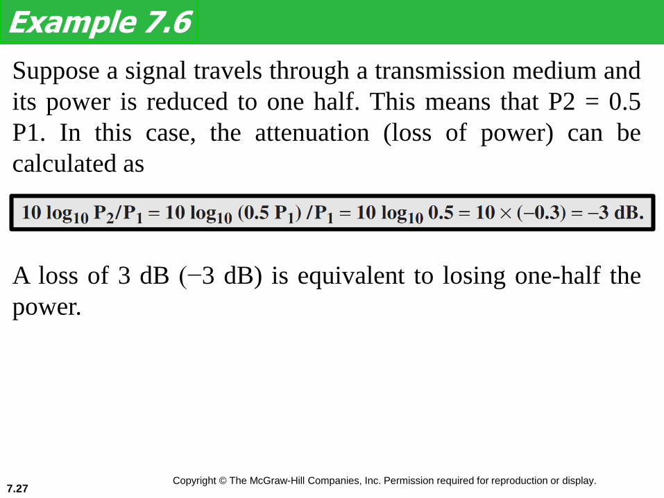
Suppose a signal travels through a transmission medium and

its power is reduced to one half. This means that P2 = 0.5

P1. In this case, the attenuation (loss of power) can be

calculated as

Example 7.6

A loss of 3 dB (−3 dB) is equivalent to losing one-half the

power.


Figure 7.14: Distortion


Figure 7.15: Noise


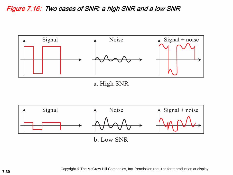
Figure 7.16: Two cases of SNR: a high SNR and a low SNR


7.1.3 Data Rate Limits

A very important consideration in data

communications is how fast we can send data, in bits

per second, over a channel. Data rate depends on

three factors:

1. The bandwidth available

2. The level of the signals we use

3. The quality of the channel (the level of noise)

Two theoretical formulas were developed to

calculate the data rate: one by Nyquist for a

noiseless channel, another by Shannon for a noisy

channel.


7.1.3 (continued)

Noiseless Channel: Nyquist Bit Rate

Noisy Channel: Shannon Capacity

Using Both Limits


We need to send 265 kbps over a noiseless (ideal) channel

with a bandwidth of 20 kHz. How many signal levels do we

need? We can use the Nyquist formula as shown:

Example 7.7

Since this result is not a power of 2, we need to either

increase the number of levels or reduce the bit rate. If we

have 128 levels, the bit rate is 280 kbps. If we have 64

levels, the bit rate is 240 kbps.


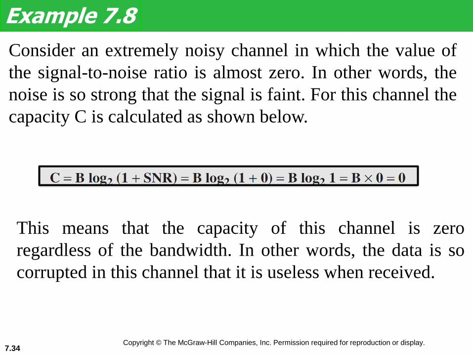
Consider an extremely noisy channel in which the value of

the signal-to-noise ratio is almost zero. In other words, the

noise is so strong that the signal is faint. For this channel the

capacity C is calculated as shown below.

Example 7.8

This means that the capacity of this channel is zero

regardless of the bandwidth. In other words, the data is so

corrupted in this channel that it is useless when received.


We can calculate the theoretical highest bit rate of a regular

telephone line. A telephone line normally has a bandwidth of

3000 Hz (300 to 3300 Hz) assigned for data

communications. The signal-to-noise ratio is usually 3162.

For this channel the capacity is calculated as shown below.

Example 7.9

This means that the highest bit rate for a telephone line is

34.881 kbps. If we want to send data faster than this, we can

either increase the bandwidth of the line or improve the

signal-to noise ratio.


We have a channel with a 1-MHz bandwidth. The SNR for

this channel is 63. What are the appropriate bit rate and

signal level?

Example 7.10


7.1.4 Performance

Up to now, we have discussed the tools of

transmitting data (signals) over a network and how

the data behave. One important issue in networking

is the performance of the network—how good is it?

We discuss quality of service, an overall

measurement of network performance, in detail in

Chapter 8.


7.1.4 (continued)

Bandwidth

Bandwidth in Hertz

Bandwidth in Bits per Seconds

Relationship

Throughput

Latency (Delay)

Bandwidth-Delay Product

Jitter


The bandwidth of a subscriber line is 4 kHz for voice or

data. The bandwidth of this line for data transmission can be

up to 56 kbps, using a sophisticated modem to change the

digital signal to analog. If the telephone company improves

the quality of the line and increases the bandwidth to 8 kHz,

we can send 112 kbps.

Example 7.11


Figure 7.17: Filling the link with bits for cases 1 and 2


We can think about the link between two points as a pipe.

The cross section of the pipe represents the bandwidth, and

the length of the pipe represents the delay. We can say the

volume of the pipe defines the bandwidth-delay product, as

shown in Figure 7.18.

Example 7.12


Figure 7.18: Concept of bandwidth-delay product


7-2 DIGITAL TRANSMISSION

A computer network is designed to sendinformation from one point to another. Thisinformation needs to be converted to either adigital signal or an analog signal fortransmission. In this section, we discuss thefirst choice, conversion to digital signals; in thenext section, we discuss the second choice,conversion to analog signals.


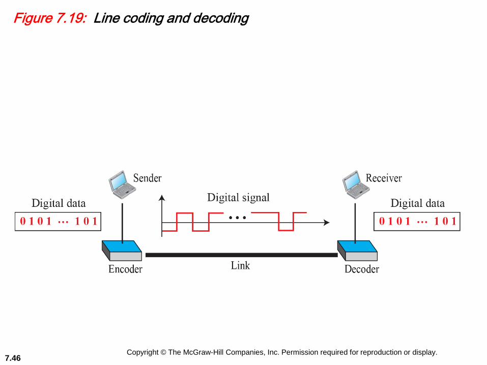
7.2.1 Digital-to-Digital Conversion

In this section, we see how we can represent

digital data by using digital signals. The

conversion involves three techniques: line

coding, block coding, and scrambling. Line

coding is always needed; block coding and

scrambling may or may not be needed.


7.2.1 (continued)

Line Coding

Polar Schemes

Bipolar Schemes

Multilevel Schemes

Block Coding

4B/5B Coding

8B/10B Coding

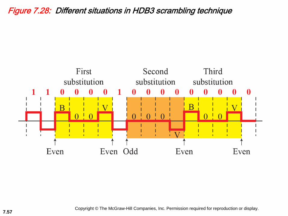
Scrambling

B8ZS Coding

HDB3 Coding


Figure 7.19: Line coding and decoding


Figure 7.20: Polar schemes (Part I: NRZ)


Figure 7.20: Polar schemes (Part II: RZ)


Figure 7.20: Polar schemes (Part III: Manchesters)


Figure 7.21: Bipolar schemes: AMI and pseudoternary


Figure 7.22: Multilevel: 2B1Q and 8B6T


Figure 7.23: Block coding concept


Figure 7.24: Using block coding 4B/5B with NRZ-I line coding scheme


Figure 7.25: 8B/10B block encoding


Figure 7.26: AMI used with scrambling


Figure 7.27: Two cases of B8ZS scrambling technique


Figure 7.28: Different situations in HDB3 scrambling technique


7.2.2 Analog-to-Digital Conversion

The techniques described in Section 7.2.1

convert digital data to digital signals.

Sometimes, however, we have an analog

signal such as one created by a microphone

or camera. The tendency today is to change

an analog signal to digital data because the

digital signal is less susceptible to noise. In

this section we describe two techniques, pulse

code modulation and delta modulation. After

the digital data are created (digitization),


7.2.2 (continued)

Pulse Code Modulation (PCM)

Sampling

Quantization

Encoding

Original Signal Recovery

PCM Bandwidth

Delta Modulation (DM)


Figure 7.29: Components of PCM encoder


Figure 7.30: Three different sampling methods for PCM


Figure 7.30: Nyquist sampling rate for low-pass and bandpass signals


Figure 7.32: Quantization and encoding of a sampled signal


64

We want to digitize the human voice. What is the bit rate,

assuming 8 bits per sample?

Solution

The human voice normally contains frequencies from 0 to

4000 Hz. So the sampling rate and bit rate are calculated as

follows.

Example 7.13


Figure 7.33: Components of a PCM decoder


Figure 7.34: The process of delta modulation


7-3 ANALOG TRANSMISSION

While digital transmission is desirable, itneeds a low-pass channel; analogtransmission is the only choice if we have abandpass channel. Converting digital data toa bandpass analog signal is traditionallycalled digital-to-analog conversion.Converting a low-pass analog signal to abandpass analog signal is traditionally calledanalog-to-analog conversion.


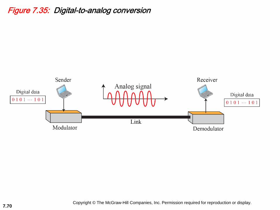
7.3.1 Digital-to-Analog Conversion

Digital-to-analog conversion is the process of

changing one of the characteristics of an analog

signal based on the information in digital data.

Figure 7.35 shows the relationship between the

digital information, the digital-to-analog

modulating process, and the resultant analog

signal.


7.3.1 (continued)

Amplitude Shift Keying

Binary ASK (BASK)

Multilevel ASK

Binary FSK (BFSK)

Multilevel FSK

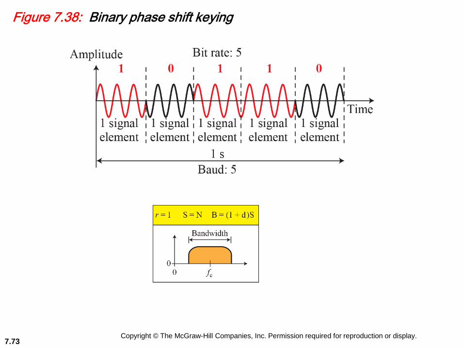
Phase Shift Keying

Binary PSK (BPSK)

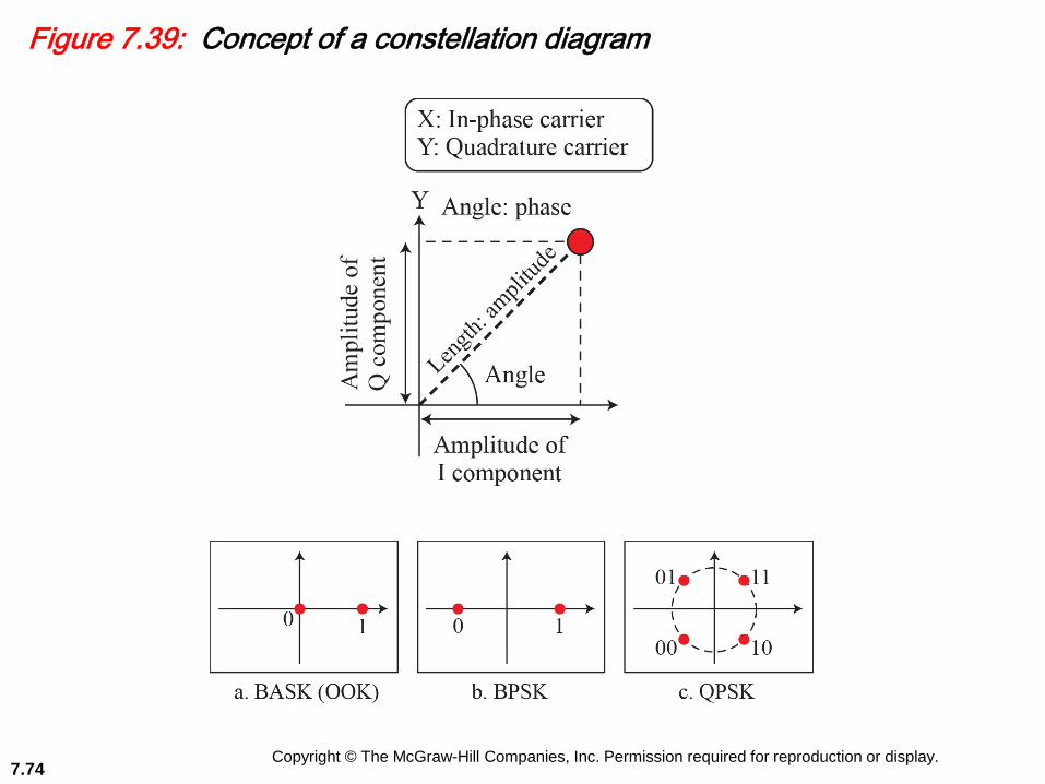
Quadrature PSK (QPSK)

Constellation Diagram

Quadrature Amplitude Modulation

Bandwidth for QAM


Figure 7.35: Digital-to-analog conversion


Figure 7.36: Binary amplitude shift keying


Figure 7.37: Binary frequency shift keying


Figure 7.38: Binary phase shift keying


Figure 7.39: Concept of a constellation diagram


Figure 7.40: Constellation diagrams for some QAMs


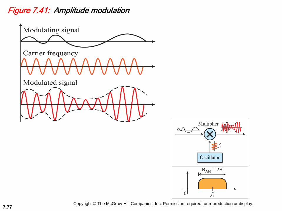
7.3.2 Analog-to-Analog Conversion

Analog-to-analog conversion, or analog

modulation, is the representation of analog

information by an analog signal. One may ask

why we need to modulate an analog signal; it is

already analog. Modulation is needed if the

medium is bandpass in nature or if only a

bandpass channel is available to us.

Amplitude Modulation

Frequency Modulation

Phase Modulation


Figure 7.41: Amplitude modulation


Figure 7.42: Frequency modulation


Figure 7.43: Phase modulation

VCO

d/dt

0fc

BPM = 2(1 + b )B


7-4 BANDWIDTH UTILIZATION

In real life, we have links with limitedbandwidths. Sometimes we need tocombine several low-bandwidth channels tomake use of one channel with a largerbandwidth. Sometimes we need to expandthe bandwidth of a channel to achieve goalssuch as privacy and anti-jamming.


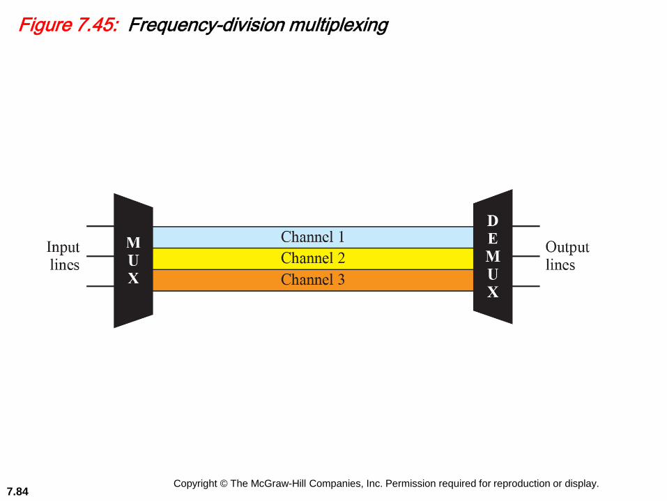
7.4.1 Multiplexing

Multiplexing is the set of techniques that allows

the simultaneous transmission of multiple signals

across a single data link. As data and

telecommunications use increases, so does traffic.

We can accommodate this increase by continuing

to add individual links each time a new channel is

needed, or we can install higher-bandwidth links

and use each to carry multiple signals.


7.4.1 (continued)

Frequency-Division Multiplexing

Wavelength-Division Multiplexing

Synchronous TDM

Statistical Time-Division Multiplexing

Time-Division Multiplexing


Figure 7.44: Dividing a link into channels


Figure 7.45: Frequency-division multiplexing


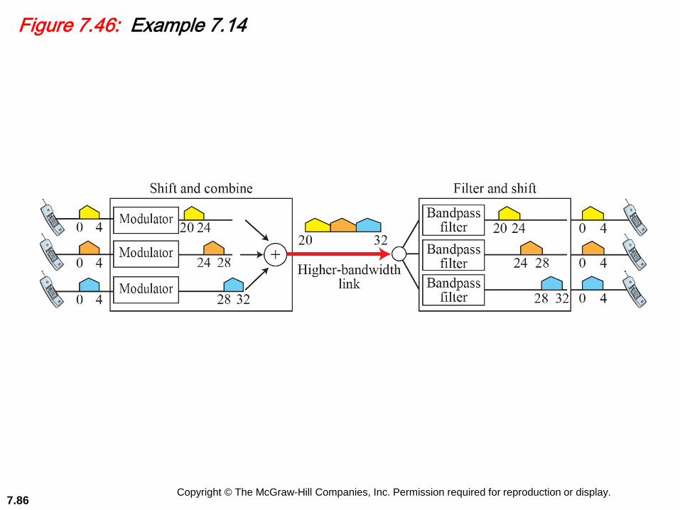
Assume that a voice channel occupies a bandwidth of 4 kHz.

We need to combine three voice channels into a link with a

bandwidth of 12 kHz, from 20 to 32 kHz. Show the

configuration, using the frequency domain. Assume there

are no guard bands.

Example 7.14


Figure 7.46: Example 7.14


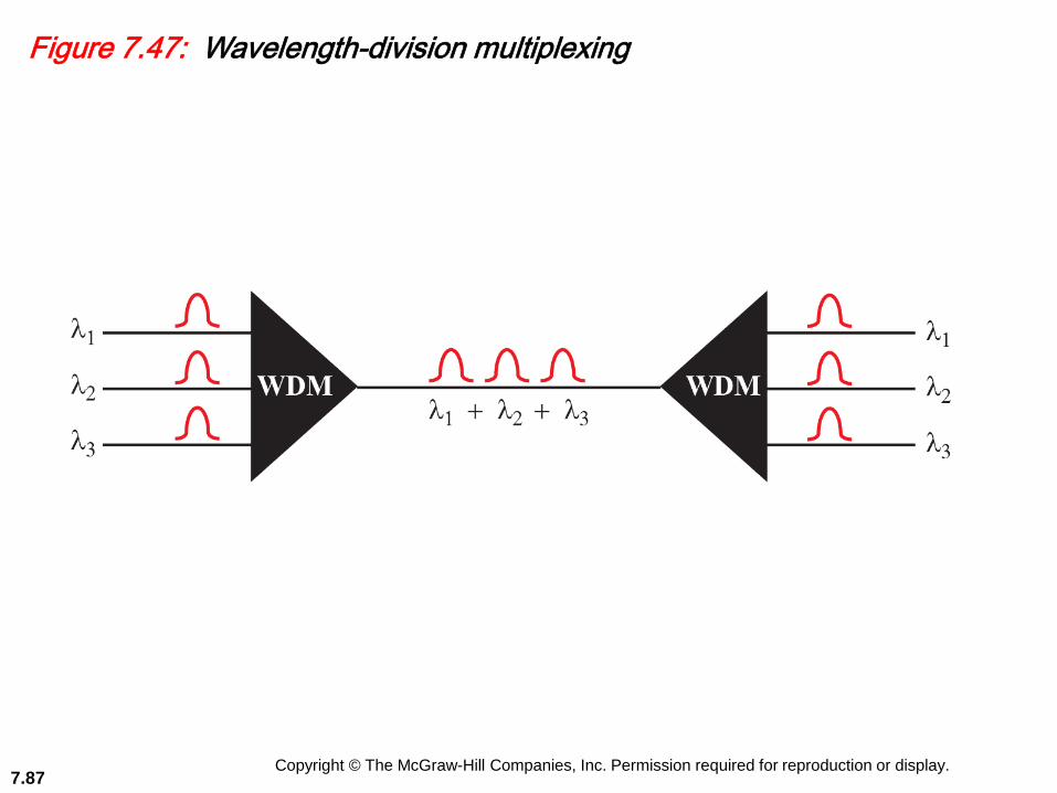
Figure 7.47: Wavelength-division multiplexing


Figure 7.48: TDM


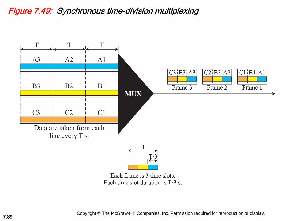
Figure 7.49: Synchronous time-division multiplexing


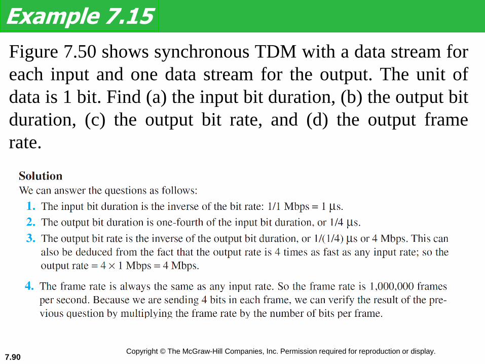
Figure 7.50 shows synchronous TDM with a data stream for

each input and one data stream for the output. The unit of

data is 1 bit. Find (a) the input bit duration, (b) the output bit

duration, (c) the output bit rate, and (d) the output frame

rate.

Example 7.15


Figure 7.50: Example 7.15


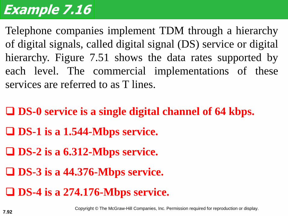
Telephone companies implement TDM through a hierarchy

of digital signals, called digital signal (DS) service or digital

hierarchy. Figure 7.51 shows the data rates supported by

each level. The commercial implementations of these

services are referred to as T lines.

Example 7.16

❑ DS-0 service is a single digital channel of 64 kbps.

❑ DS-1 is a 1.544-Mbps service.





Figure 7.51: Digital hierarchy


Figure 7.52: TDM slot comparison


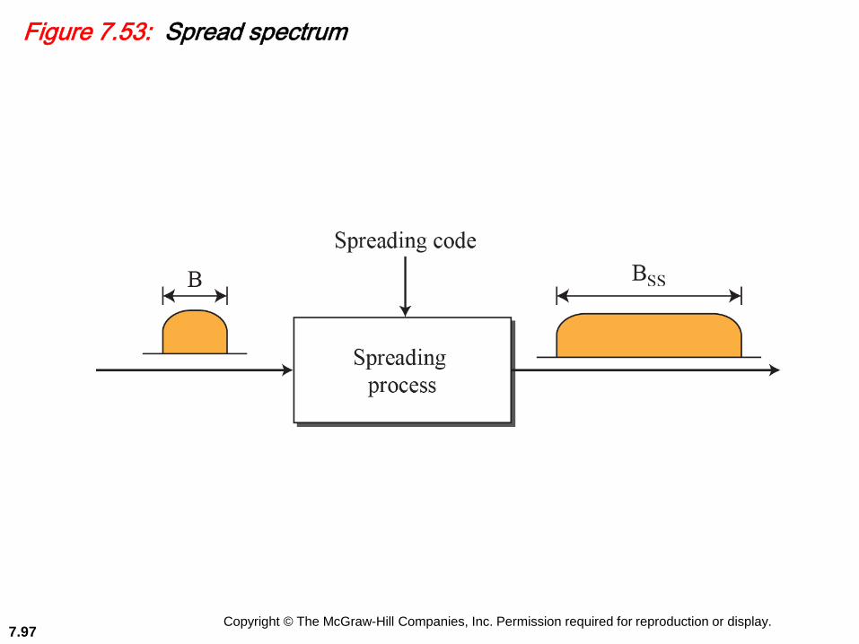
7.4.2 Spread Spectrum

In spread spectrum, we also combine signals from

different sources to fit into a larger bandwidth, but

our goals are somewhat different. In these types of

applications, we have some concerns that

outweigh bandwidth efficiency. In wireless

applications, all stations use air (or a vacuum) as

the medium for communication. Stations must be

able to share this medium without interception by

an eavesdropper and without being subject to

jamming from a malicious intruder (in military

operations, for example).


7.4.2 (continued)

Frequency Hopping Spread Spectrum (FHSS)

Bandwidth Sharing

Direct Sequence Spread Spectrum


Figure 7.53: Spread spectrum


Figure 7.54: Frequency hopping spread spectrum (FHSS)


Figure 7.55: FHSS cycles


Figure 7.56: Bandwidth sharing


Figure 7.57: DSSS


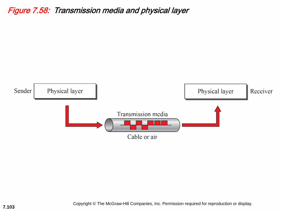
7-5 TRANSMISSION MEDIA

We discussed many issues related to thephysical layer in this chapter. In this section,we discuss transmission media.Transmission media are actually locatedbelow the physical layer and are directlycontrolled by the physical layer. We couldsay that transmission media belong to layerzero.


Figure 7.58: Transmission media and physical layer


7.5.1 Guided Media

Guided media, which are those that provide a

conduit from one device to another, include

twisted-pair cable, coaxial cable, and fiber-optic

cable. A signal traveling along any of these media

is directed and contained by the physical limits of

the medium. Twisted-pair and coaxial cable use

metallic (copper) conductors that accept and

transport signals in the form of electric current.

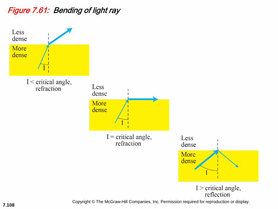
Fiber-optic cable is a cable that accepts and

transports signals in the form of light.


7.5.1 (continued)

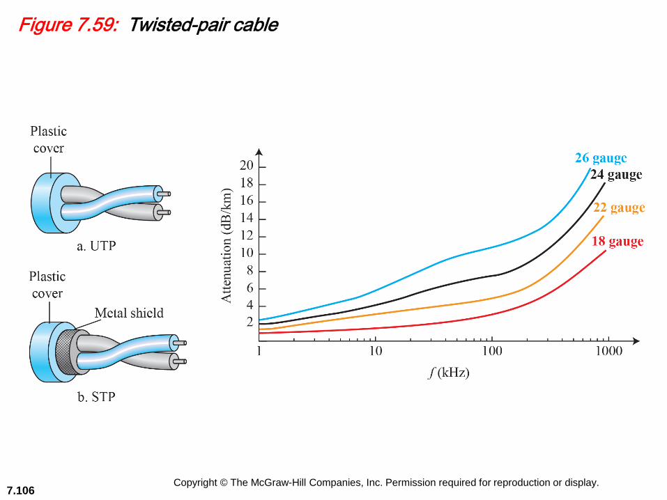
Twisted-Pair Cable

Performance

Applications

Coaxial Cable

Performance

Applications

Fiber-Optic Cable

Propagation Modes

Performance

Applications


Figure 7.59: Twisted-pair cable


Figure 7.60: Coaxial cable


Figure 7.61: Bending of light ray


Figure 7.62: Optical fiber


Figure 7.63: Modes


7.5.2 Unguided Media

Unguided media transport electromagnetic waves

without using a physical conductor. This type of

communication is often referred to as wireless

communication. Signals are normally broadcast

through free space and thus are available to

anyone who has a device capable of receiving

them.

Radio Waves

Microwaves

Infrared


Figure 7.64: Electromagnetic spectrum for wireless communication


Table 7.1: Bands


Chapter 7: Summary

Data must be transformed to electromagnetic signals to be

transmitted. Analog data are continuous and take continuous

values. Digital data have discrete states and take discrete values.

Analog signals can have an infinite number of values in a

range; digital signals can have only a limited number of values.

In data communications, we commonly use periodic analog

signals and non-periodic digital signals.

Digital-to-digital conversion involves three techniques: line

coding, block coding, and scrambling. The most common

technique to change an analog signal to digital data

(digitization) is called pulse code modulation (PCM).


Chapter 7: Summary (continued)

Digital-to-analog conversion is the process of changing one of

the characteristics of an analog signal based on the information

in the digital data. Digital-to-analog can be achieved in several

ways: ASK, FSK, and PSK. QAM combines ASK and PSK.

Analog-to-analog conversion can be accomplished in three

ways: AM, FM), and PM.

Bandwidth utilization is the use of available bandwidth to

achieve specific goals. Efficiency can be achieved by using

multiplexing; privacy and anti-jamming can be achieved by

using spreading.

Transmission media lie below the physical layer. We discussed

guided and unguided media.

Documents

Chapter 7 Physical Layer and Transmission Media...7.1.2 Transmission Impairment Signals travel through transmission media, which are not perfect. The imperfection causes signal impairment