Chapter 6

Linear Programming: The Simplex Method

Section 3

The Dual Problem: Minimization with Problem Constraints of the Form ≥

2

Learning Objectives for Section 6.3

The student will be able to formulate the dual problem. The student will be able to solve minimization problems. The student will be able to solve applications of the dual

such as the transportation problem. The student will be able to summarize problem types and

solution methods.

Dual Problem: Minimization with Problem Constraints of the Form >

3

Dual Problem: Minimization With Problem Constraints of the Form >

Associated with each minimization problem with > constraints is a maximization problem called the dual problem. The dual problem will be illustrated through an example. We wish to minimize the objective function C subject to certain constraints:

C 16x1 9x

2 21x

3

x1 x

2 3x

312

2x1 x

2 x

316

x1, x

2,x

30

4

Initial Matrix

We start with an initial matrix A which corresponds to the problem constraints:

A

1 1 3 12

2 1 1 16

16 9 21 1

5

Transpose of Matrix A

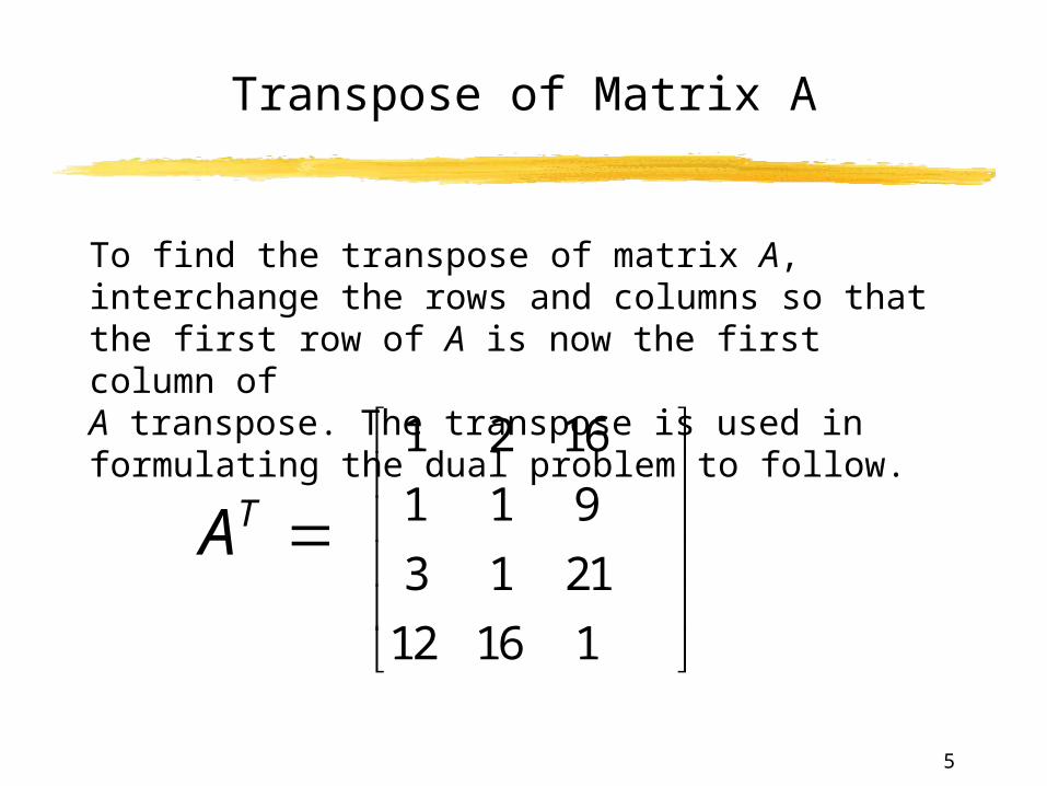
To find the transpose of matrix A, interchange the rows and columns so that the first row of A is now the first column of A transpose. The transpose is used in formulating the dual problem to follow.

1 2 16

1 1 9

3 1 21

12 16 1

AT

6

Dual of the Minimization Problem

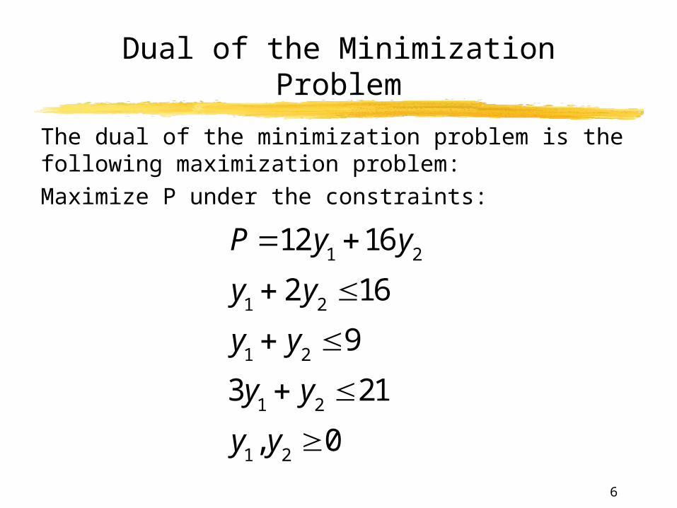
The dual of the minimization problem is the following maximization problem:

Maximize P under the constraints:

P 12y116y

2

y1 2y

216

y1 y

29

3y1 y

221

y1, y

20

7

Formation of the Dual Problem

Given a minimization problem with ≥ problem constraints,

1. Use the coefficients and constants in the problem constraints and the objective function to form a matrix A with the coefficients of the objective function in the last row.

2. Interchange the rows and columns of matrix A to form the matrix AT, the transpose of A.

3. Use the rows of AT to form a maximization problem with ≤ problem constraints.

8

Theorem 1: Fundamental Principle of Duality

A minimization problem has a solution if and only if its dual problem has a solution. If a solution exists, then the optimal value of the minimization problem is the same as the optimum value of the dual problem.

9

Forming the Dual Problem

We transform the inequalities into equalities by adding the slack variables x1, x2, x3:

y1 2y

2 x

116

y1 y

2 x

29

3y1 y

2 x

321

12y1 16y

2 p 0

10

Form the Simplex Tableau for the Dual Problem

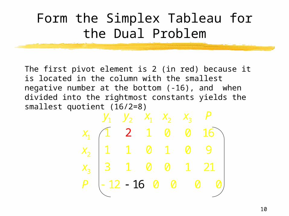
The first pivot element is 2 (in red) because it is located in the column with the smallest negative number at the bottom (-16), and when divided into the rightmost constants yields the smallest quotient (16/2=8)

1 2 1 2 3

1

2

3

1 1 0 0 16

1 1 0 1 0 9

3 1 0 0 1 21

1

2

0612 0 0 0

y y x x x P

x

x

x

P

11

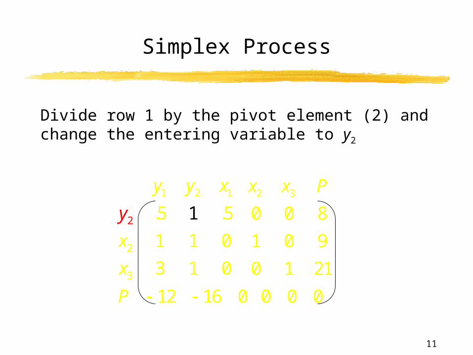
Simplex Process

Divide row 1 by the pivot element (2) and change the entering variable to y2

1 2 1 2 3

2

3

2 .5 .5 0 0 8

1 1 0 1 0 9

3 1 0

1

0 1 21

12 16 0 0 0 0

y y x x x P

y

x

x

P

12

Simplex Process(continued)

Perform row operations to get zeros in the column containing the pivot element. Result is shown below.Identify the next pivot element (0.5) (in red)

1 2 1 2 3

2

3

2 .5 1 .5 0 0 8

0 .5 1 0 1

2.5 0 .5 0 1 13

0 8 0 0 14 28

.5

y y x

P

y

x x P

x

x

New pivot element

Pivot element located in this column because of negative indicator

13

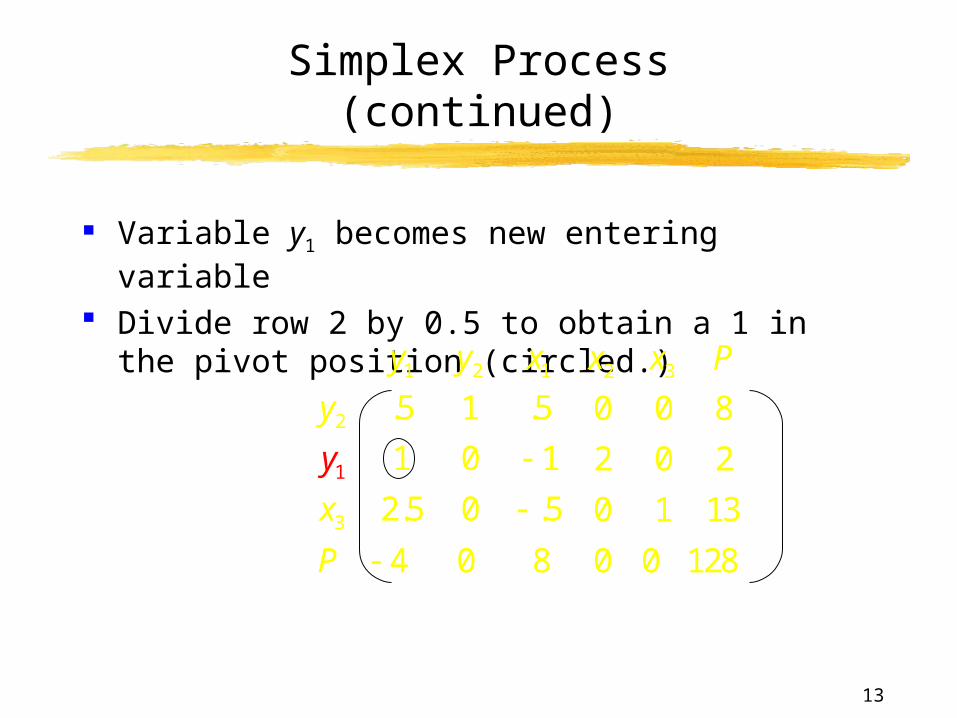
Simplex Process(continued)

Variable y1 becomes new entering variable

Divide row 2 by 0.5 to obtain a 1 in the pivot position (circled.)

1 2 1 2 3

2

3

1

.5 1 .5 0 0 8

1 0 1 2 0 2

2.5 0 .5 0 1 13

4 0 8 0 0 128

y y x x x P

y

P

y

x

14

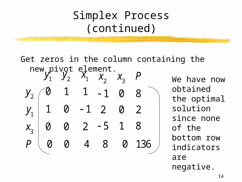
Simplex Process(continued)

Get zeros in the column containing the new pivot element.

y1

y2

x1

y2

0 1 1

y1

1 0 1

x3

0 0 2

x2

x3

P

1 0 8

2 0 2

5 1 8

P 0 0 4 8 0 136

We have now obtained the optimal solution since none of the bottom row indicators are negative.

15

Solution of the Linear Programming Problem

Solution: An optimal solution to a minimization problem can always be obtained from the bottom row of the final simplex tableau for the dual problem.

Minimum of P is 136, which is also the maximum of the dual problem. It occurs at x1 = 4, x2 = 8, x3 = 0

1 2 1 2 3

2

1

3

0 1 1 1 0 8

1 0 1 2 0 2

0 0 2

0 0 4 8 0 13

5 1 8

6

y y x x x P

P

y

y

x

16

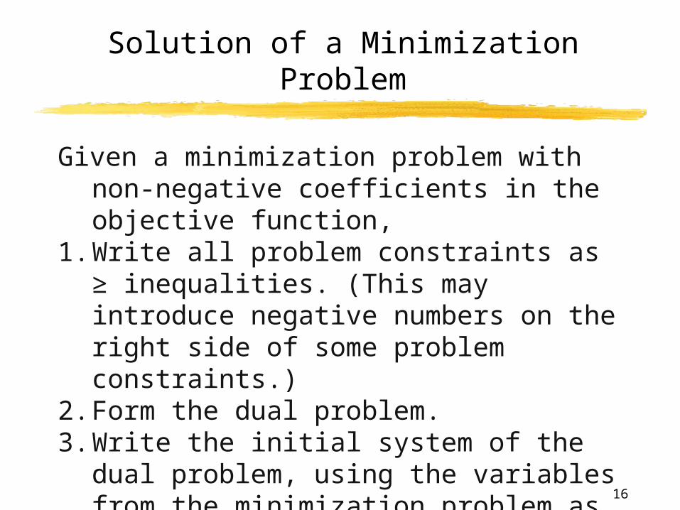
Solution of a Minimization Problem

Given a minimization problem with non-negative coefficients in the objective function,

1. Write all problem constraints as ≥ inequalities. (This may introduce negative numbers on the right side of some problem constraints.)

2. Form the dual problem.3. Write the initial system of the dual problem, using

the variables from the minimization problem as slack variables.

17

Solution of a Minimization Problem

4. Use the simplex method to solve the dual problem.

5. Read the solution of the minimization problem from the bottom row of the final simplex tableau in step 4.

Note: If the dual problem has no optimal solution, the minimization problem has no optimal solution.

18

Application:Transportation Problem

One of the first applications of linear programming was to the problem of minimizing the cost of transporting materials. Problems of this type are referred to as transportation problems.

Example: A computer manufacturing company has two assembly plants, plant A and plant B, and two distribution outlets, outlet I and outlet II. Plant A can assemble at most 700 computers a month, and plant B can assemble at most 900 computers a month. Outlet I must have at least 500 computers a month, and outlet II must have at least 1,000 computers a month.

19

Transportation Problem (continued)

Transportation costs for shipping one computer from each plant to each outlet are as follows: $6 from plant A to outlet I; $5 from plant A to outlet II: $4 from plant B to outlet I; $8 from plant B to outlet II. Find a shipping schedule that will minimize the total cost of shipping the computers from the assembly plants to the distribution outlets. What is the minimum cost?

20

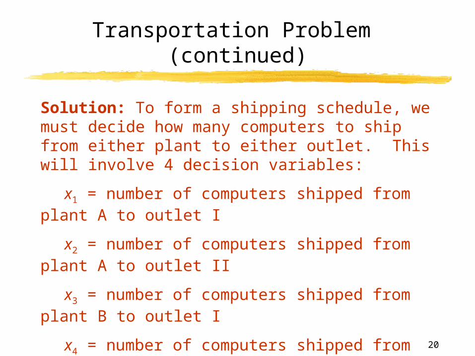
Transportation Problem (continued)

Solution: To form a shipping schedule, we must decide how many computers to ship from either plant to either outlet. This will involve 4 decision variables:

x1 = number of computers shipped from plant A to outlet I

x2 = number of computers shipped from plant A to outlet II

x3 = number of computers shipped from plant B to outlet I

x4 = number of computers shipped from plant B to outlet II

21

Transportation Problem (continued)

Constraints are as follows:

x1 + x2 < 700 Available from A

x3 + x4 < 900 Available from B

x1 + x3 > 500 Required at I

x2 + x4 > 1,000 Required at II

Total shipping charges are:

C = 6x1 + 5x2 + 4x3 + 8x4

22

Transportation Problem (continued)

Thus, we must solve the following linear programming problem:

Minimize C = 6x1 + 5x2 + 4x3 + 8x4

subject to

x1 + x2 < 700 Available from A

x3 + x4 < 900 Available from B

x1 + x3 > 500 Required at I

x2 + x4 > 1,000 Required at II

Before we can solve this problem, we must multiply the first two constraints by -1 so that all are of the > type.

23

Transportation Problem (continued)

The problem can now be stated as:

Minimize C = 6x1 + 5x2 + 4x3 + 8x4

subject to

-x1 - x2 > -700

- x3 - x4 > -900

x1 + x3 > 500

x2 + x4 > 1,000

x1, x2, x3, x4 > 0

24

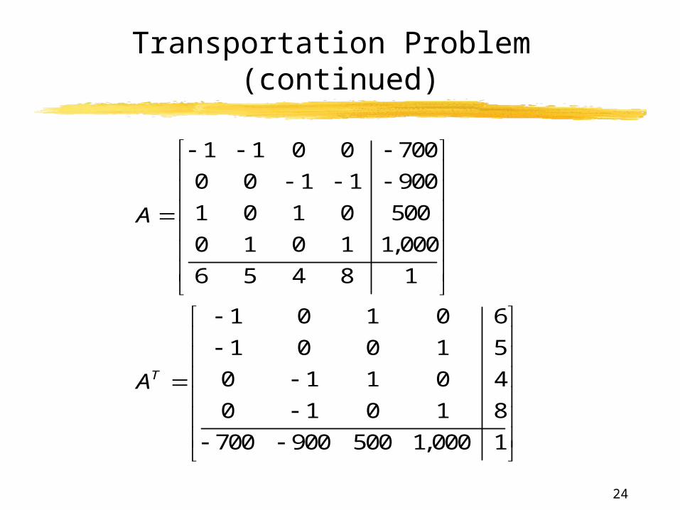
Transportation Problem (continued)

1 1 0 0 700

0 0 1 1 900

1 0 1 0 500

0 1 0 1 1,000

6 5 4 8 1

1 0 1 0 6

1 0 0 1 5

0 1 1 0 4

0 1 0 1 8

700 900 500 1,000 1

T

A

A

25

Transportation Problem (continued)

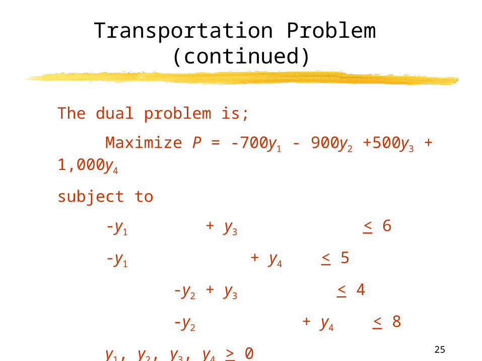
The dual problem is;

Maximize P = -700y1 - 900y2 +500y3 + 1,000y4

subject to

-y1 + y3 < 6

-y1 + y4 < 5

-y2 + y3 < 4

-y2 + y4 < 8

y1, y2, y3, y4 > 0

26

Transportation Problem (continued)

Introduce slack variables x1, x2, x3, and x4 to form the initial system for the dual:

-y1 + y3 + x1 = 6

-y1 + y4 + x2 = 5

-y2 + y3 + x3 = 4

-y2 + y4 + x4 = 8

-700y1 - 900y2 +500y3 + 1,000y4 +P = 0

27

Transportation Problem Solution

If we form the simplex tableau for this initial system and solve, we find that the shipping schedule that minimizes the shipping charges is 0 from plant A to outlet I, 700 from plant A to outlet II, 500 from plant B to outlet I, and 300 from plant B to outlet II. The total shipping cost is $7,900.

28

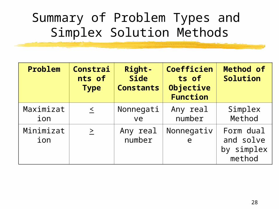
Summary of Problem Types and Simplex Solution Methods

Problem Constraints of Type

Right-Side Constants

Coefficients of Objective Function

Method of Solution

Maximization < Nonnegative Any real number

Simplex Method

Minimization > Any real number

Nonnegative Form dual and solve by

simplex method