Quasi-Newton minimization for the p(x)-Laplacianproblem

M. Caliaria,∗, S. Zucchera

aDepartment of Computer Science, University of Verona, Strada Le Grazie 15, 37134Verona, Italy

Abstract

We propose a quasi-Newton minimization approach for the solution of the p(x)-Laplacian elliptic problem, x ∈ Ω ⊂ Rm. This method outperforms those exist-ing for the p(x)-variable case, which are based on general purpose minimizerssuch as BFGS. Moreover, when compared to ad hoc techniques available in lit-erature for the p-constant case, and usually referred to as “mesh independent”,the present method turns out to be generally superior thanks to better descentdirections given by the quadratic model.

Keywords: p(x)-Laplacian, degenerate quasi-linear elliptic problem,quasi-Newton minimization

1. Introduction

We consider the p(x)-Laplacian elliptic problem−div(|∇u(x)|p(x)−2∇u(x)) = f(x) x ∈ Ω ⊂ Rm,u(x) = 0 x ∈ ∂Ω

(1)

where Ω is an open bounded subset of Rm with ∂Ω Lipschitz continuous, p ∈P log, that is p is a measurable function, p : Ω → [1,+∞] and 1/p is globallylog-Holder continuous. Moreover, we assume 1 < pmin ≤ p(x) ≤ pmax < ∞,f ∈ Lp′(x)(Ω) (where p′(x) denotes the dual variable exponent of p(x)) and u ∈V = W

1,p(x)0 (Ω). Since p(x) is bounded, we may see the space W

1,p(x)0 (Ω) as the

space of functions in W 1,p(x)(Ω) with null trace on ∂Ω. The trace operator canbe defined on W 1,p(x)(Ω) in such a way that, as usual, if u ∈W 1,p(x)(Ω)∩C(Ω),then its trace coincides with u|∂Ω. We refer to [1] for a general introduction tovariable exponent Sobolev spaces. This model occurs in many applications, suchas image processing [2, 3] and electrorheological fluids [4–6], in which p(x) mayassume values close to the extreme ones [7–9]. Hereafter we leave the explicitdependence on x ∈ Ω ⊂ Rm only for the exponent p(x) and all integrals are

∗Corresponding author

Preprint submitted to Elsevier June 20, 2016

intended over the domain Ω. The p(x)-Laplacian problem (1) admits a unique[10] weak solution u satisfying

u = arg minv∈V

J(v)

where

J(u) =

∫ |∇u|p(x)

p(x)−∫fu (2)

or, equivalently,J ′(u)v = 0, ∀v ∈ V (3)

where

J ′(u)v =

∫|∇u|p(x)−2∇u · ∇v −

∫fv. (4)

A common way [11–14] to tackle the problem is the direct minimization, in asuitable finite dimensional subspace of V , of the functional J in equation (2),rather than solving the nonlinear equation (3) [15]. However, to our knowl-edge, ad hoc minimization algorithms were developed only for the p-constantcase [13–15], whereas only general purpose methods such as the quasi-Newtonmethod BFGS (Broyden–Fletcher–Goldfarb–Shanno) have been used for thep(x)-variable case [12].

In this work we minimize J(u) employing a new quadratic model whichmakes use of the exact second differential J ′′(u), only slightly regularized inorder to handle possible analytic or numerical degeneracy when |∇u| is smalland p(x) is close to the extreme values pmin or pmax. The result is an efficientand robust algorithm converging faster than those available in literature, bothfor the p-constant case and the p(x)-variable one.

2. Minimization problem

We minimize J(u) in a suitable finite element subspace of V and we call uh

the solution

uh = arg minvh∈V h0

J(vh)⇔ J ′(uh)vh = 0 ∀vh ∈ V h0 .

Given a regular triangulation of a polygonal approximation Ωh of the domain,we select the subspace V h0 ⊂ V of continuous piecewise linear functions whichare zero at the boundaries of Ωh. Since for p 6= 2 problem (1) is degenerate quasi-linear elliptic, its solution has a limited regularity (see, for instance, [16]) andtherefore higher-order finite element approximations do not worth (see Ref. [17]).For the variable exponent case, p(x) is approximated by continuous piecewiselinear functions as well, even if a local approximation by constant functions ispossible (see Ref. [10, 18]). Given the approximation un ∈ V h0 of the solutionuh at iteration n, we look for a direction dn ∈ V h0 such that

J(un + αndn) < J(un).

2

The descent direction dn is called steepest descent direction if

J ′(un)dn = −‖J ′(un)‖∗ ‖dn‖

where ‖·‖ is a suitable norm in V h0 and ‖·‖∗ its dual norm. The idea (seeRef. [13, 14]) is to find dn as the solution of

dn : bn(dn, v) = −J ′(un)v, ∀v ∈ V h0where bn(·, ·) is a suitable bilinear form depending on iteration n. The choice ofbn characterizes the minimization method.

The extension to non-homogeneous Dirichlet boundary conditions is straight-

forward. The solution u belongs to the variable exponent Sobolev spaceW1,p(x)g =

v ∈ W 1,p(x) : v = g on ∂Ω and its piecewise approximation must be in thespace V hgh , that is the space of continuous piecewise linear functions whose valueof ∂Ωh is gh, where gh is chosen to approximate the Dirichlet boundary data.The search directions are still in the space V h0 .

2.1. Gradient-based directions

The choice in Ref. [13], for the p-constant case, is dn = wn, where

bn(wn, v) =

∫

(ε+ |∇un|p−2)∇wn · ∇v, p > 2∫

(ε+ |∇un|)p−2∇wn · ∇v, p < 2.

(5)

The bilinear form bn(·, ·) corresponds to a simple linearization of J ′(un)v. Theparameter ε is introduced in order to handle possible analytic or numerical de-generacy where |∇un| is small. In fact, for p 2 the term |∇un|p−2

mayunderflow even if |∇un| > 0. On the other hand, for p < 2 the same termmay overflow. We notice that the parameter ε is introduced only for findingthe descent direction and not for regularizing the original p(x)-Laplacian func-tional J . With the above choice, the authors in Ref. [13] proved a convergenceresult (J(un)→ J(u)) only for the case p > 2. Their complicated proof is hardlyextendible to the case p < 2 or to the general case with variable p(x). The di-rection wn is called in Ref. [13] preconditioned steepest descent. The scalar valueαn is chosen as

αn = arg minαJ(un + αdn) (6)

(exact linesearch).In Ref. [14] wn is computed for all 1 < p < +∞ using the first definition

in (5). The descent direction is then computed by

dn = wn + βndn−1

where

βn = max

0,min

wnTwn

wn−1Twn−1,

(wn − wn−1)Twn

wn−1Twn−1

.

3

The definition of βn corresponds to an hybridization of the popular Fletcher–Reeves and Polak–Ribiere–Polyak parameters for the nonlinear conjugate gra-dient method (see also Ref. [19]). Direction dn is called in Ref. [14] hybridconjugate gradient. The scalar αn is chosen as in equation (6).

2.2. Quasi-Newton directionOur proposal for the direction dn in the general case p(x) is the following.

We start with the second differential of J , which is well defined for p(x) ≥ 2

J ′′(u)(v, w) =

∫(p(x)− 2)|∇u|p(x)−4(∇u · ∇w)(∇u · ∇v) +

∫|∇u|p(x)−2∇w · ∇v (7a)

=

∫|∇u|p(x)−2

((p(x)− 2)

∇u|∇u|

· ∇w∇u|∇u|

· ∇v +∇w · ∇v)

(7b)

=

∫|∇u|p(x)−2

((p(x)− 2) (Sign(∇u) · ∇w) (Sign(∇u) · ∇v) +∇w · ∇v

)(7c)

where we defined

Sign(∇u(x)) =∇u(x)√

|∇u(x)|2 +(

1− sign(|∇u(x)|2)) =

∇u(x)

|∇u(x)| if ∇u(x) 6= 0

0 if ∇u(x) = 0

Formula (7c) is well defined and numerically computable for p(x) ≥ 2 even if∇u(x) is zero somewhere. On the other hand it is in general still not positivedefinite and not defined if p(x) < 2 and ∇u(x) = 0 somewhere. Therefore we

modify |∇u|p(x)−2in formula (7c) into

|∇u|p(x)−2ε = ε+

(ε2 ·

(1− sign(|∇u|2)

)+ |∇u|2

) p(x)−22

. (8)

In this way, we accomplish both the regularizations in equation (5), since p(x)can be simultaneously very large in some regions and small in some other regions.Hence, the regularized second differential is

J ′′ε (u)(v, w) =

∫|∇u|p(x)−2

ε

((p(x)− 2) (Sign(∇u) · ∇w) (Sign(∇u) · ∇v) +∇w · ∇v

). (9)

Therefore our descent direction is dn = wn defined by

wn : bn(wn, v) = −J ′(un)v, ∀v ∈ V h0 (10)

where bn(wn, v) = J ′′ε (un)(wn, v). In this way, we are in practice approximatingJ(u) by a quadratic positive definite model

J(u) ≈ J(un) + J ′(un)(u− un) +1

2J ′′ε (un)((u− un), (u− un))

from which the name quasi-Newton. Other regularizations would be possible,

by replacing |∇u|p(x)−2with

ε+ (ε+ |∇u|)p(x)−2

4

(see, for instance, [13]) or with

ε+(ε2 + |∇u|2

) p(x)−22

(see, for instance, [20]), which is similar to the idea used in [21], where theproblem itself, and not only the second differential, is regularized in the sameway. Our choice (8) turned out to be the most effective in the numerical exper-iments. We notice that the choice of the gradient-based directions [13, 14] canbe generalized for the p(x)-variable case as

wn : Pε(un)(wn, v) =

∫|∇un|p(x)−2

ε ∇wn · ∇v = −J ′(un)v, ∀v ∈ V h0 (11)

and

dn = wn, preconditioned steepest descent [13] (12a)

dn = wn + βndn−1, hybrid conjugate gradient [14]. (12b)

The scaling length αn in un+αndn is found by a backtracking line search method

based on sufficient decrease condition (Armijo’s rule). Together with reasonableassumptions on J ′′ε (un), this is enough to guarantee convergence to a stationarypoint of J(u) (see, for instance, [22, Th. 3.2.4]).

3. Numerical examples

We implemented the quasi-Newton and, for comparison, the gradient-basedminimization method [14] in FreeFem++ 3.31 [23] for the solution of two-dimensional problems, being the extension to three dimensions straightforward.The numerical solution at iteration n is denoted by

un(x, y) =∑j

unj φj(x, y)

where φj(x, y) is the j-th nodal finite element basis function. In the followingnumerical examples, the initial guess u0(x, y) is always the solution of Poisson’sproblem corresponding to p = 2. The descent directions wn in (10) and (11)are approximated by the linear conjugate gradient method.

The exit criterion (see Ref. [24, p. 160]) is

maxj

∣∣∣∣J ′(un)φj unjJ(un)

∣∣∣∣ ≤ 10−6

where J ′(un)φj is defined in (4) and denotes Hadamard’s product. For com-parison, in Ref. [13, 14] the initial guess is u0(x, y) = 0, wn is computed by amultigrid solver, the bisection method and the golden section method are usedin the linesearch, respectively and the exit criterion is√

bn(dn, dn)√b0(d0, d0)

≤ 10−6.

5

The solution of equation (10) is obtained by the default linear conjugategradient method provided by FreeFem++, which employs the diagonal pre-conditioner. We also tried the matrix of entries Pε(u

n)(φj , φi) (see (11)) aspreconditioner, since it is an approximation of the matrix J ′′ε (un)(φj , φi) usedfor the quasi-Newton direction. In this way, in general, we observed a smallernumber of iterations needed for the convergence of the linear conjugate gradientmethod. However this approach never paid in terms of total CPU time due tothe cost of the factorization of the preconditioner.

In the next tables, we report the total number of minimization iterations,the CPU time, the relative error of J and of the approximated solution in theW 1,p norm

‖u‖W 1,p =

(∫|u|p

) 1p

+

(∫|∇u|p

) 1p

whenever the exact solution is known. In case of variable p(x), we report eitherthe Luxemburg norm in Lp(x), that is

‖u‖Lp(x) = infγ>0

γ :

∫Ω

∣∣∣∣u(x)

γ

∣∣∣∣p(x)

dx ≤ 1

or in W 1,p(x), that is

‖u‖W 1,p(x) = ‖u‖Lp(x) + ‖∇u‖Lp(x) .

We have to say that the CPU time here shown, taken on an Intel Quad Corei7-4600U 2.10GHz, is not a reliable measure of the computational effort, since inour experiments we sometimes found significant variations in different instancesof the same experiment1.

3.1. p-constant case

Example 1. This case is taken from Ref. [13, 14], with Ω = B(0, 1) and f = 1.The exact solution is

u(x, y) =p− 1

p

(1

2

) 1p−1 (

1− (x2 + y2)p

2p−2

)and the corresponding value of J(u) is

J(u) = π

(1

2

) 1p−1 (p− 1)2

p(2− 3p).

The disk B(0, 1) is discretized with four different meshes called D1, D2, D3 andD4 with number of vertices (dof) 1600, 6221, 24444 and 97451 respectively. The

1All the next numerical experiments are reproducible with the code available at the webpage http://profs.scienze.univr.it/caliari/software.htm.

6

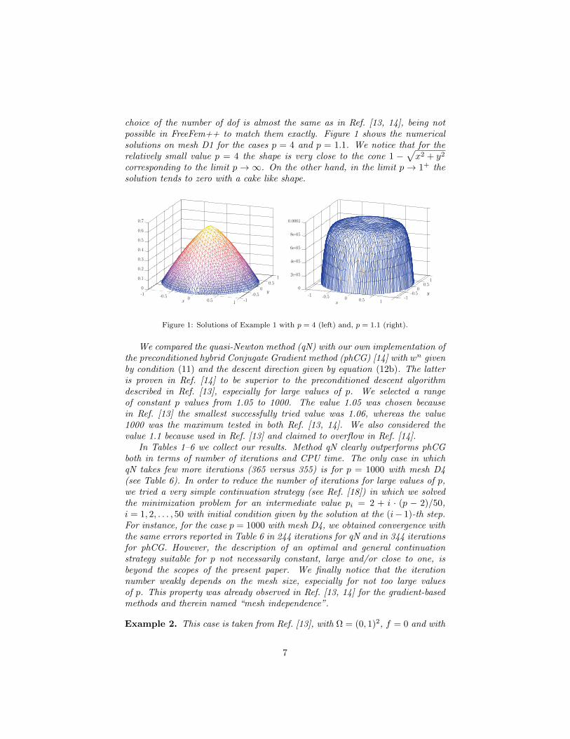
choice of the number of dof is almost the same as in Ref. [13, 14], being notpossible in FreeFem++ to match them exactly. Figure 1 shows the numericalsolutions on mesh D1 for the cases p = 4 and p = 1.1. We notice that for therelatively small value p = 4 the shape is very close to the cone 1 −

√x2 + y2

corresponding to the limit p→∞. On the other hand, in the limit p→ 1+ thesolution tends to zero with a cake like shape.

-0.5x

0 0.5 1

-1

-1

0

0.1

0.2

0.3

0.4

0.5

0.6

0.7

y

10.5

0-0.5 -1 -0.5

x0 0.5 1

0

2e-05

4e-05

6e-05

8e-05

0.0001

y

10.5

0-0.5

-1

Figure 1: Solutions of Example 1 with p = 4 (left) and, p = 1.1 (right).

We compared the quasi-Newton method (qN) with our own implementation ofthe preconditioned hybrid Conjugate Gradient method (phCG) [14] with wn givenby condition (11) and the descent direction given by equation (12b). The latteris proven in Ref. [14] to be superior to the preconditioned descent algorithmdescribed in Ref. [13], especially for large values of p. We selected a rangeof constant p values from 1.05 to 1000. The value 1.05 was chosen becausein Ref. [13] the smallest successfully tried value was 1.06, whereas the value1000 was the maximum tested in both Ref. [13, 14]. We also considered thevalue 1.1 because used in Ref. [13] and claimed to overflow in Ref. [14].

In Tables 1–6 we collect our results. Method qN clearly outperforms phCGboth in terms of number of iterations and CPU time. The only case in whichqN takes few more iterations (365 versus 355) is for p = 1000 with mesh D4(see Table 6). In order to reduce the number of iterations for large values of p,we tried a very simple continuation strategy (see Ref. [18]) in which we solvedthe minimization problem for an intermediate value pi = 2 + i · (p − 2)/50,i = 1, 2, . . . , 50 with initial condition given by the solution at the (i− 1)-th step.For instance, for the case p = 1000 with mesh D4, we obtained convergence withthe same errors reported in Table 6 in 244 iterations for qN and in 344 iterationsfor phCG. However, the description of an optimal and general continuationstrategy suitable for p not necessarily constant, large and/or close to one, isbeyond the scopes of the present paper. We finally notice that the iterationnumber weakly depends on the mesh size, especially for not too large valuesof p. This property was already observed in Ref. [13, 14] for the gradient-basedmethods and therein named “mesh independence”.

Example 2. This case is taken from Ref. [13], with Ω = (0, 1)2, f = 0 and with

7

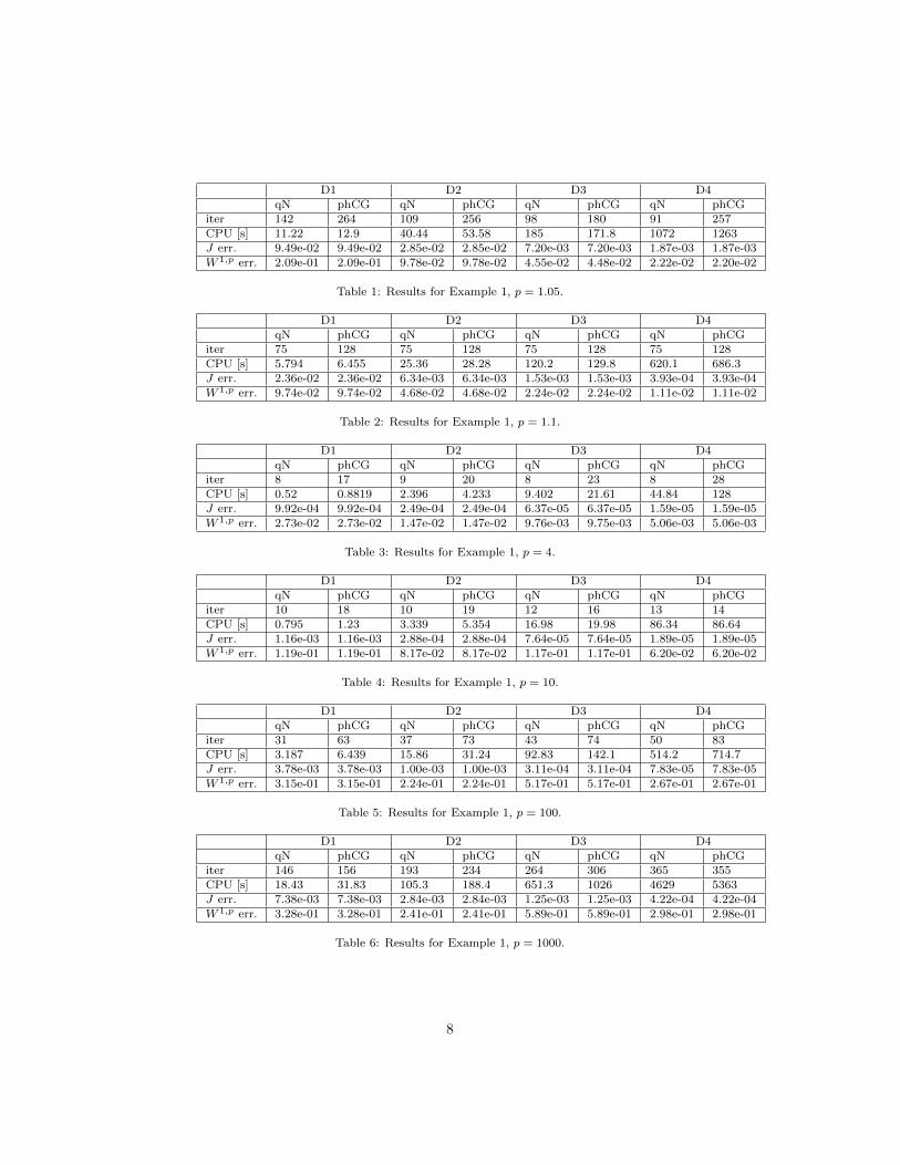
D1 D2 D3 D4qN phCG qN phCG qN phCG qN phCG

iter 142 264 109 256 98 180 91 257CPU [s] 11.22 12.9 40.44 53.58 185 171.8 1072 1263J err. 9.49e-02 9.49e-02 2.85e-02 2.85e-02 7.20e-03 7.20e-03 1.87e-03 1.87e-03W 1,p err. 2.09e-01 2.09e-01 9.78e-02 9.78e-02 4.55e-02 4.48e-02 2.22e-02 2.20e-02

Table 1: Results for Example 1, p = 1.05.

D1 D2 D3 D4qN phCG qN phCG qN phCG qN phCG

iter 75 128 75 128 75 128 75 128CPU [s] 5.794 6.455 25.36 28.28 120.2 129.8 620.1 686.3J err. 2.36e-02 2.36e-02 6.34e-03 6.34e-03 1.53e-03 1.53e-03 3.93e-04 3.93e-04W 1,p err. 9.74e-02 9.74e-02 4.68e-02 4.68e-02 2.24e-02 2.24e-02 1.11e-02 1.11e-02

Table 2: Results for Example 1, p = 1.1.

D1 D2 D3 D4qN phCG qN phCG qN phCG qN phCG

iter 8 17 9 20 8 23 8 28CPU [s] 0.52 0.8819 2.396 4.233 9.402 21.61 44.84 128J err. 9.92e-04 9.92e-04 2.49e-04 2.49e-04 6.37e-05 6.37e-05 1.59e-05 1.59e-05W 1,p err. 2.73e-02 2.73e-02 1.47e-02 1.47e-02 9.76e-03 9.75e-03 5.06e-03 5.06e-03

Table 3: Results for Example 1, p = 4.

D1 D2 D3 D4qN phCG qN phCG qN phCG qN phCG

iter 10 18 10 19 12 16 13 14CPU [s] 0.795 1.23 3.339 5.354 16.98 19.98 86.34 86.64J err. 1.16e-03 1.16e-03 2.88e-04 2.88e-04 7.64e-05 7.64e-05 1.89e-05 1.89e-05W 1,p err. 1.19e-01 1.19e-01 8.17e-02 8.17e-02 1.17e-01 1.17e-01 6.20e-02 6.20e-02

Table 4: Results for Example 1, p = 10.

D1 D2 D3 D4qN phCG qN phCG qN phCG qN phCG

iter 31 63 37 73 43 74 50 83CPU [s] 3.187 6.439 15.86 31.24 92.83 142.1 514.2 714.7J err. 3.78e-03 3.78e-03 1.00e-03 1.00e-03 3.11e-04 3.11e-04 7.83e-05 7.83e-05W 1,p err. 3.15e-01 3.15e-01 2.24e-01 2.24e-01 5.17e-01 5.17e-01 2.67e-01 2.67e-01

Table 5: Results for Example 1, p = 100.

D1 D2 D3 D4qN phCG qN phCG qN phCG qN phCG

iter 146 156 193 234 264 306 365 355CPU [s] 18.43 31.83 105.3 188.4 651.3 1026 4629 5363J err. 7.38e-03 7.38e-03 2.84e-03 2.84e-03 1.25e-03 1.25e-03 4.22e-04 4.22e-04W 1,p err. 3.28e-01 3.28e-01 2.41e-01 2.41e-01 5.89e-01 5.89e-01 2.98e-01 2.98e-01

Table 6: Results for Example 1, p = 1000.

8

non-homogeneous Dirichlet boundary conditions such that the exact solution is

u(x, y) = (x2 + y2)p−22p−2 .

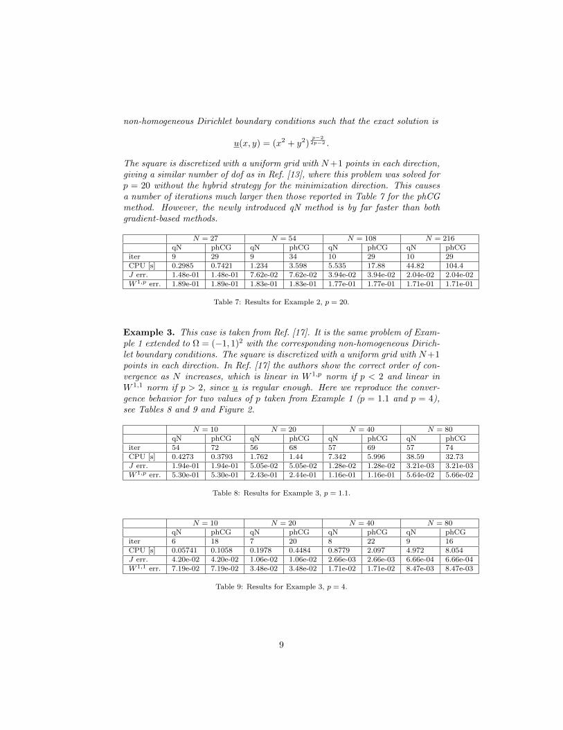
The square is discretized with a uniform grid with N+1 points in each direction,giving a similar number of dof as in Ref. [13], where this problem was solved forp = 20 without the hybrid strategy for the minimization direction. This causesa number of iterations much larger then those reported in Table 7 for the phCGmethod. However, the newly introduced qN method is by far faster than bothgradient-based methods.

N = 27 N = 54 N = 108 N = 216qN phCG qN phCG qN phCG qN phCG

iter 9 29 9 34 10 29 10 29CPU [s] 0.2985 0.7421 1.234 3.598 5.535 17.88 44.82 104.4J err. 1.48e-01 1.48e-01 7.62e-02 7.62e-02 3.94e-02 3.94e-02 2.04e-02 2.04e-02W 1,p err. 1.89e-01 1.89e-01 1.83e-01 1.83e-01 1.77e-01 1.77e-01 1.71e-01 1.71e-01

Table 7: Results for Example 2, p = 20.

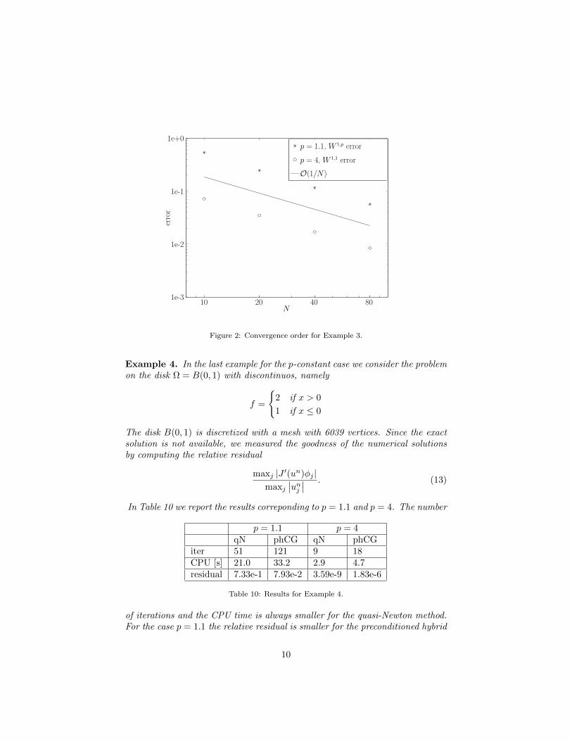
Example 3. This case is taken from Ref. [17]. It is the same problem of Exam-ple 1 extended to Ω = (−1, 1)2 with the corresponding non-homogeneous Dirich-let boundary conditions. The square is discretized with a uniform grid with N+1points in each direction. In Ref. [17] the authors show the correct order of con-vergence as N increases, which is linear in W 1,p norm if p < 2 and linear inW 1,1 norm if p > 2, since u is regular enough. Here we reproduce the conver-gence behavior for two values of p taken from Example 1 (p = 1.1 and p = 4),see Tables 8 and 9 and Figure 2.

N = 10 N = 20 N = 40 N = 80qN phCG qN phCG qN phCG qN phCG

iter 54 72 56 68 57 69 57 74CPU [s] 0.4273 0.3793 1.762 1.44 7.342 5.996 38.59 32.73J err. 1.94e-01 1.94e-01 5.05e-02 5.05e-02 1.28e-02 1.28e-02 3.21e-03 3.21e-03W 1,p err. 5.30e-01 5.30e-01 2.43e-01 2.44e-01 1.16e-01 1.16e-01 5.64e-02 5.66e-02

Table 8: Results for Example 3, p = 1.1.

N = 10 N = 20 N = 40 N = 80qN phCG qN phCG qN phCG qN phCG

iter 6 18 7 20 8 22 9 16CPU [s] 0.05741 0.1058 0.1978 0.4484 0.8779 2.097 4.972 8.054J err. 4.20e-02 4.20e-02 1.06e-02 1.06e-02 2.66e-03 2.66e-03 6.66e-04 6.66e-04W 1,1 err. 7.19e-02 7.19e-02 3.48e-02 3.48e-02 1.71e-02 1.71e-02 8.47e-03 8.47e-03

Table 9: Results for Example 3, p = 4.

9

10 20 40 801e-3

1e-2

1e-1

1e+0

N

error

p = 1.1, W 1,p error

p = 4, W 1,1 error

O(1/N)

Figure 2: Convergence order for Example 3.

Example 4. In the last example for the p-constant case we consider the problemon the disk Ω = B(0, 1) with discontinuos, namely

f =

2 if x > 0

1 if x ≤ 0

The disk B(0, 1) is discretized with a mesh with 6039 vertices. Since the exactsolution is not available, we measured the goodness of the numerical solutionsby computing the relative residual

maxj |J ′(un)φj |maxj

∣∣unj ∣∣ . (13)

In Table 10 we report the results correponding to p = 1.1 and p = 4. The number

p = 1.1 p = 4qN phCG qN phCG

iter 51 121 9 18CPU [s] 21.0 33.2 2.9 4.7residual 7.33e-1 7.93e-2 3.59e-9 1.83e-6

Table 10: Results for Example 4.

of iterations and the CPU time is always smaller for the quasi-Newton method.For the case p = 1.1 the relative residual is smaller for the preconditioned hybrid

10

Conjugate Gradient method. Compared with all the previous results, this couldbe due to the residual (13) not being a good indicator of the error for solutionswith low regularity and in the case p < 2.

3.2. p(x)-variable case

Example 5. This case is the two-dimensional extension of the one-dimensionalexample reported in Ref. [12], with Ω = (−1, 1)2, f = 0 and

p(x, y) =

1−εε |x|+ 1 + ε if |x| ≤ ε

2 if ε < |x| ≤ 1

where ε is a small parameter and p(0, y) → 1+ when ε → 0+. The non-homogeneous Dirichlet boundary conditions are such that the exact solution is

u(x, y) =

(U(|x|)− U(0)) · sign(x) if |x| ≤ ε(C(|x| − 1) +B) · sign(x) if ε < |x| ≤ 1

where C is set to 1.3, and, for 0 ≤ x ≤ ε,

U(x) =

(1−εε x+ ε

)exp

(lnC

1−εε x+ε

)− lnC · Ei

(lnC

1−εε x+ε

)1−εε

and B = U(ε)−U(0) +C(1− ε). The function Ei(x) is the exponential integraldefined as

Ei(x) = −∫ ∞−x

e−t

tdt.

For small values of ε the solution has a steep gradient along x = 0. For in-stance, for ε = 0.02, ∂xu(0, y) = C

1ε = 1.350 ≈ 5 · 105. As correctly observed

in Ref. [12], a more efficient and accurate finite element approximation wouldrequire a discontinuous Galerkin approach. For this reason, in Tables 11 and12, we report the Luxemburg norm in Lp(x) space of the relative error. In fact,even if the solution is in W 1,p(x) space, due to the steep gradient along x = 0,we had no reliable numerical approximation of ‖∇u‖Lp(x) on the uniform gridwe used (N = 101 points in each direction).

Tables 11 and 12 show that for relatively small values of ε the quasi-Newtonmethod takes only three iterations. On the other hand, if we use the BFGSmethod implemented in FreeFem++ (the same method was chosen by the authorsin Ref. [12] for the one-dimensional example), then the maximum number ofallowed iterations is reached and the CPU time is much larger. The hybridpreconditioned Conjugate Gradient method, never applied before to the p(x)-Laplacian, is better than BFGS but in any case worse than our quasi-Newtonmethod.

11

qN phCG BFGSiter 3 13 50CPU [s] 2.9007 5.56235 121.529

Lp(x) error 9.66e-02 9.67e-02 1.05e-01

Table 11: Results for Example 5, ε = 0.04.

qN phCG BFGSiter 3 5 50CPU [s] 3.9337 4.72026 128.144

Lp(x) error 3.92e-01 3.92e-01 4.03e-01

Table 12: Results for Example 5, ε = 0.02.

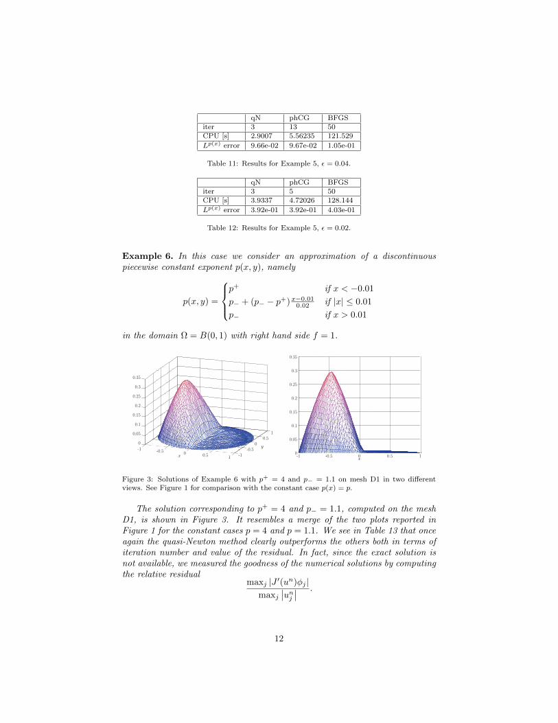
Example 6. In this case we consider an approximation of a discontinuouspiecewise constant exponent p(x, y), namely

p(x, y) =

p+ if x < −0.01

p− + (p− − p+)x−0.010.02 if |x| ≤ 0.01

p− if x > 0.01

in the domain Ω = B(0, 1) with right hand side f = 1.

-0.5x

0 0.5 1

-1

-1

0

0.05

0.1

0.15

0.2

0.25

0.3

0.35

y0

0.51

-0.5

-1 -0.5 0 0.5x

0

0.05

0.1

0.15

0.2

0.25

0.3

0.35

1

Figure 3: Solutions of Example 6 with p+ = 4 and p− = 1.1 on mesh D1 in two differentviews. See Figure 1 for comparison with the constant case p(x) = p.

The solution corresponding to p+ = 4 and p− = 1.1, computed on the meshD1, is shown in Figure 3. It resembles a merge of the two plots reported inFigure 1 for the constant cases p = 4 and p = 1.1. We see in Table 13 that onceagain the quasi-Newton method clearly outperforms the others both in terms ofiteration number and value of the residual. In fact, since the exact solution isnot available, we measured the goodness of the numerical solutions by computingthe relative residual

maxj |J ′(un)φj |maxj

∣∣unj ∣∣ .

12

qN phCG BFGSiter 18 44 50CPU [s] 1.891 3.247 8.758residual 1.39e-06 2.00e-05 2.49e-01

Table 13: Results for Example 6, p+ = 4, p− = 1.1.

Example 7. This case is taken from Ref. [11], with Ω = (−1, 1)2, f = 0 and

p(x, y) = 1 +

(1

2(x+ y) + 2

)−1

.

The corresponding exact solution is

u(x, y) =√

2e2(e

12 (x+y) − 1

).

N = 20 N = 40 N = 60 N = 80 N = 100 N = 120iter qN 3 3 3 3 2 2CPU [s] 0.07415 0.2949 1.382 2.563 1.686 2.87J err. 1.11e-03 2.77e-04 1.23e-04 6.93e-05 4.44e-05 3.08e-05

W 1,p(x) err. 2.19e-02 1.08e-02 7.16e-03 5.36e-03 4.30e-03 3.58e-03

Table 14: Results for Example 7.

20 40 60 80 100 1201e-3

1e-2

1e-1

N

error

W 1,p(x) error

O(1/N)

Figure 4: Convergence order for Example 7.

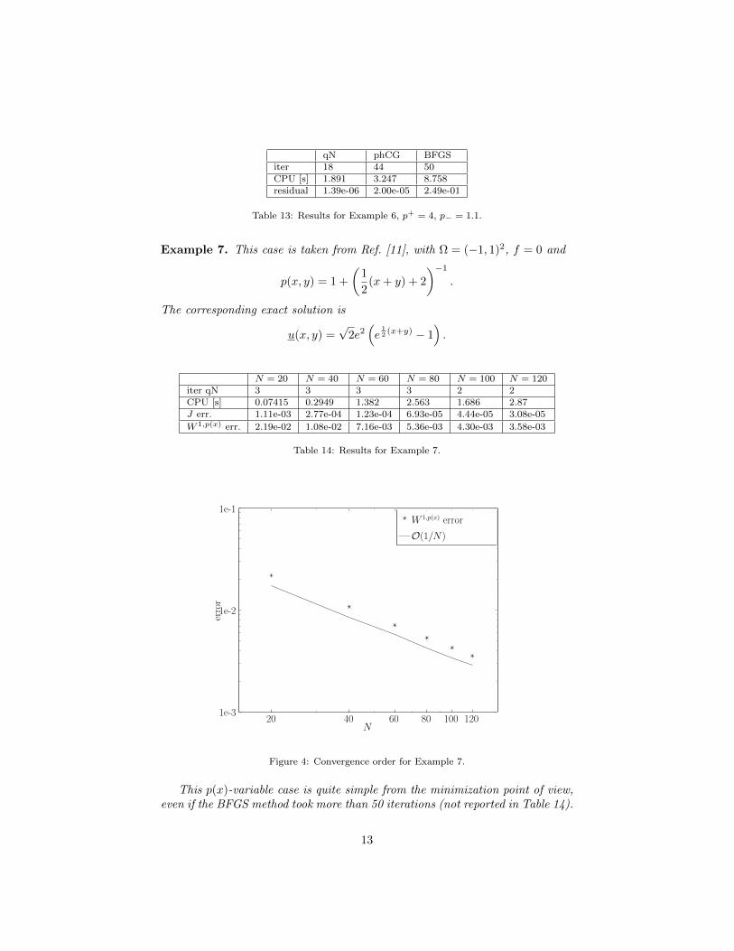
This p(x)-variable case is quite simple from the minimization point of view,even if the BFGS method took more than 50 iterations (not reported in Table 14).

13

As shown in Ref. [11], the correct linear order in N of the error in W 1,p(x) normis achieved (see Figure 4), where N+1 is the number of points for each directionof the uniform grid on the square Ω.

4. Conclusions

We developed a minimization approach for the p(x)-Laplacian problem basedon a quadratic model of the objective functional with a regularized second dif-ferential (quasi-Newton minimization). We have carried out several numericalexamples in two space dimensions with constant p or variable p(x), verified theresults against existing analytic solutions, and found that our method outper-forms those available in literature, both in number of iterations and CPU time.In particular, the quasi-Newton approach proved to be robust and efficient forvalues of p very small (up to 1.05) or very large (up to 1000) and for examplesof p(x) varying on the domain in a range between p1 and p2 with 1.02 ≤ p1 < 2and 2 ≤ p2 ≤ 4.

[1] L. Diening, P. Harjulehto, P. Hasto, M. Ruzicka, Lebesgue and SobolevSpaces with Variable Exponents, Vol. 2017 of Lect. Notes Math., Springer,2011.

[2] Y. Chen, S. Levine, M. Rao, Variable Exponent, Linear Growth Functionalsin Image Restoragion, SIAM J. Appl. Math. 66 (4) (2006) 1383–1406.

[3] P. Harjulehto, P. P. Hasto, U. V. Le, M. Nuortio, Overview of differentialequations with non-standard growth, Nonlinear Anal. 72 (2010) 4551–4574.

[4] K. Rajagopal, M. Ruzicka, On the modeling of electrorheological materials,Mech. Res. Commun. 23 (4) (1996) 401–407.

[5] M. Ruzicka, Electrorheological Fluids: Modeling and Mathematical The-ory, Vol. 1748 of Lect. Notes Math., Springer-Verlag, Berlin, 2000.

[6] L. C. Berselli, D. Breit, L. Diening, Convergence analysis for a finite elementapproximation of a steady model for electrorheological fluids, Numer. Math.132 (2016) 657–689.

[7] J. W. Barrett, L. Prigozhin, Beans critical-state model as p → ∞ limit ofan evolutionary p-Laplacian equation, Nonlinear Anal. 42 (2000) 977–993.

[8] E. M. Bollt, R. Chartrand, S. Esedoglu, P. Schultz, K. R. Vixie, Graduatedadaptive image denoising: local compromise between total variation andisotropic diffusion, Adv. Comput. Math. 31 (2009) 61–85.

[9] G. Bouchitte, G. Buttazzo, L. De Pascale, A p-Laplacian Approximationfor Some Mass Optimization Problems, J. Optim. Theory Appl. 118 (2003)1–25.

14

[10] D. Breit, L. Diening, S. Schwarzacher, Finite element approximation of thep(x)-Laplacian, SIAM J. Numer. Anal. 53 (1) (2015) 551–572.

[11] L. M. Del Pezzo, S. Martınez, Order of convergence of the finite elementmethod for the p(x)-Laplacian, IMA J. Numer. Anal. 35 (4) (2015) 1864–1887.

[12] L. M. Del Pezzo, A. L. Lombardi, S. Martınez, Interior penalty discontin-uous Galerkin FEM for the p(x)-Laplacian, SIAM J. Numer. Anal. 50 (5)(2012) 2497–2521.

[13] Y. Q. Huang, R. Li, W. Liu, Preconditioned descent algorithms for p-Laplacian, J. Sci. Comput. 32 (2) (2007) 343–371.

[14] G. Zhou, Y. Huang, C. Feng, Preconditioned hybrid conjugate gradientalgorithm for p-Laplacian, Int. J. Numer. Anal. Model. 2 (Supp.) (2005)123–130.

[15] R. Bermejo, J.-A. Infante, A multigrid algorithm for the p-Laplacian, SIAMJ. Sci. Comput. 21 (5) (2000) 1774–1789.

[16] T. Iwaniec, J. J. Manfredi, Regularity of p-harmonic functions on the plane,Rev. Mat. Iberoamericana 5 (1–2) (1989) 1–19.

[17] J. W. Barrett, W. B. Liu, Finite element approximation of the p-Laplacian,Math. Comp. 61 (204) (1993) 523–537.

[18] M. Caliari, S. Zuccher, The inverse power method for the p(x)-Laplacianproblem, J. Sci. Comput. 65 (2) (2015) 698–714.

[19] S. Babaie-Kafaki, R. Ghanbari, A hybridization of the Polak–Ribiere–Polyak and Fletcher–Reeves conjugate gradient methods, Numer. Algo-ritms 68 (2015) 481–495.

[20] R. J. Biezuner, J. Brown, G. Ercole, E. M. Martins, Computing the FirstEigenpair of the p-Laplacian via Inverse Iteration of Sublinear Supersolu-tions, J. Sci. Comput. 52 (1) (2012) 180–201.

[21] A. Hirn, Finite element approximation of singular power-law systems,Math. Comp. 82 (283) (2013) 1247–1268.

[22] C. T. Kelley, Iterative Methods for Optimization, Vol. 18 of Frontiers inApplied Mathematics, SIAM, Philadelphia, 1999.

[23] F. Hecht, New development in FreeFem++, J. Numer. Math. 20 (3-4)(2012) 251–265.

[24] J. E. Dennis, R. B. Schnabel, Numerical Methods for Unconstrained Opti-mization and Nonlinear Equations, Vol. 16 of Classics in Applied Mathe-matics, SIAM, Philadelphia, PA, USA, 1996.

15