Embed Size (px)
Citation preview

DATABASESYSTEMSGROUP
Knowledge Discovery in Databases I: Classification 1
Knowledge Discovery in DatabasesSS 2016
Lecture: Prof. Dr. Thomas Seidl
Tutorials: Julian Busch, Evgeniy Faerman, Florian Richter, Klaus Schmid
Ludwig-Maximilians-Universität MünchenInstitut für InformatikLehr- und Forschungseinheit für Datenbanksysteme
Chapter 6: Classification

DATABASESYSTEMSGROUP
Chapter 5: Classification
1) Introduction– Classification problem, evaluation of classifiers, numerical prediction
2) Bayesian Classifiers– Bayes classifier, naive Bayes classifier, applications
3) Linear discriminant functions & SVM1) Linear discriminant functions
2) Support Vector Machines
3) Non-linear spaces and kernel methods
4) Decision Tree Classifiers– Basic notions, split strategies, overfitting, pruning of decision trees
5) Nearest Neighbor Classifier– Basic notions, choice of parameters, applications
6) Ensemble Classification
Outline 2

DATABASESYSTEMSGROUP
Additional literature for this chapter
• Christopher M. Bishop: Pattern Recognition and Machine Learning. Springer, Berlin 2006.
Classification Introduction 3

DATABASESYSTEMSGROUP
Introduction: Example
• Training data
• Simple classifierif age > 50 then risk = low;
if age ≤ 50 and car type = truck then risk = low;
if age ≤ 50 and car type ≠ truck then risk = high.
Classification Introduction 4
ID age car type risk1 23 family high2 17 sportive high3 43 sportive high4 68 family low5 32 truck low
DATABASESYSTEMSGROUP
Classification: Training Phase (Model Construction)
Classification Introduction 5
Classifier
(age=60, familiy)if age > 50 then risk = low;
if age ≤ 50 and car type = truck then risk = low;
if age ≤ 50 and car type ≠ truck then risk = high
ID age car type risk1 23 family high2 17 sportive high3 43 sportive high4 68 family low5 32 truck low
training data
classifier
training
unknown data
class label

DATABASESYSTEMSGROUP
Classification: Prediction Phase (Application)
Classification Introduction 6
Classifier
(age=60, family) risk = lowif age > 50 then risk = low;
if age ≤ 50 and car type = truck then risk = low;
if age ≤ 50 and car type ≠ truck then risk = high
training data
classifier
training
unknown data
class label
ID age car type risk1 23 family high2 17 sportive high3 43 sportive high4 68 family low5 32 truck low

DATABASESYSTEMSGROUP
Classification
• The systematic assignment of new observations to known categories according to criteria learned from a training set
• Formally, – a classifier K for a model 𝑀𝑀(𝜃𝜃) is a function 𝐾𝐾𝑀𝑀(𝜃𝜃): 𝐷𝐷 → 𝑌𝑌, where
• 𝐷𝐷: data space– Often d-dimensional space with attributes 𝑎𝑎𝑖𝑖, 𝑖𝑖 = 1, … ,𝑑𝑑 (not necessarily vector space)
– Some other space, e.g. metric space
• 𝑌𝑌 = 𝑦𝑦1, … ,𝑦𝑦𝑘𝑘 : set of 𝑘𝑘 distinct class labels 𝑦𝑦𝑗𝑗, 𝑗𝑗 = 1, … , 𝑘𝑘• 𝑂𝑂 ⊆ 𝐷𝐷: set of training objects, 𝑜𝑜 = (𝑜𝑜1, … , 𝑜𝑜𝑑𝑑), with known class labels 𝑦𝑦 ∈ 𝑌𝑌
– Classification: application of classifier K on objects from 𝐷𝐷 − 𝑂𝑂
• Model 𝑀𝑀(𝜃𝜃) is the “type” of the classifier, and 𝜃𝜃 are the model parameters
• Supervised learning: find/learn optimal parameters 𝜃𝜃 for the model 𝑀𝑀 𝜃𝜃 from the given training data
Classification Introduction 7
DATABASESYSTEMSGROUP
Supervised vs. Unsupervised Learning
• Unsupervised learning (clustering)– The class labels of training data are unknown– Given a set of measurements, observations, etc. with the aim of
establishing the existence of classes or clusters in the data• Classes (=clusters) are to be determined
• Supervised learning (classification)– Supervision: The training data (observations, measurements, etc.)
are accompanied by labels indicating the class of the observations• Classes are known in advance (a priori)
– New data is classified based on information extracted from the training set
Classification Introduction 8
[WK91] S. M. Weiss and C. A. Kulikowski. Computer Systems that Learn: Classification and Prediction Methods from Statistics, Neural Nets, Machine Learning, and Expert Systems. Morgan Kaufman, 1991.

DATABASESYSTEMSGROUP
Numerical Prediction
• Related problem to classification: numerical prediction– Determine the numerical value of an object
– Method: e.g., regression analysis
– Example: prediction of flight delays
• Numerical prediction is different from classification– Classification refers to predict categorical class label
– Numerical prediction models continuous-valued functions
• Numerical prediction is similar to classification– First, construct a model
– Second, use model to predict unknown value• Major method for numerical prediction is regression
– Linear and multiple regression
– Non-linear regression
Classification Introduction 9
Windspeed
Delay offlight
query
predictedvalue
DATABASESYSTEMSGROUP
Goals of this lecture
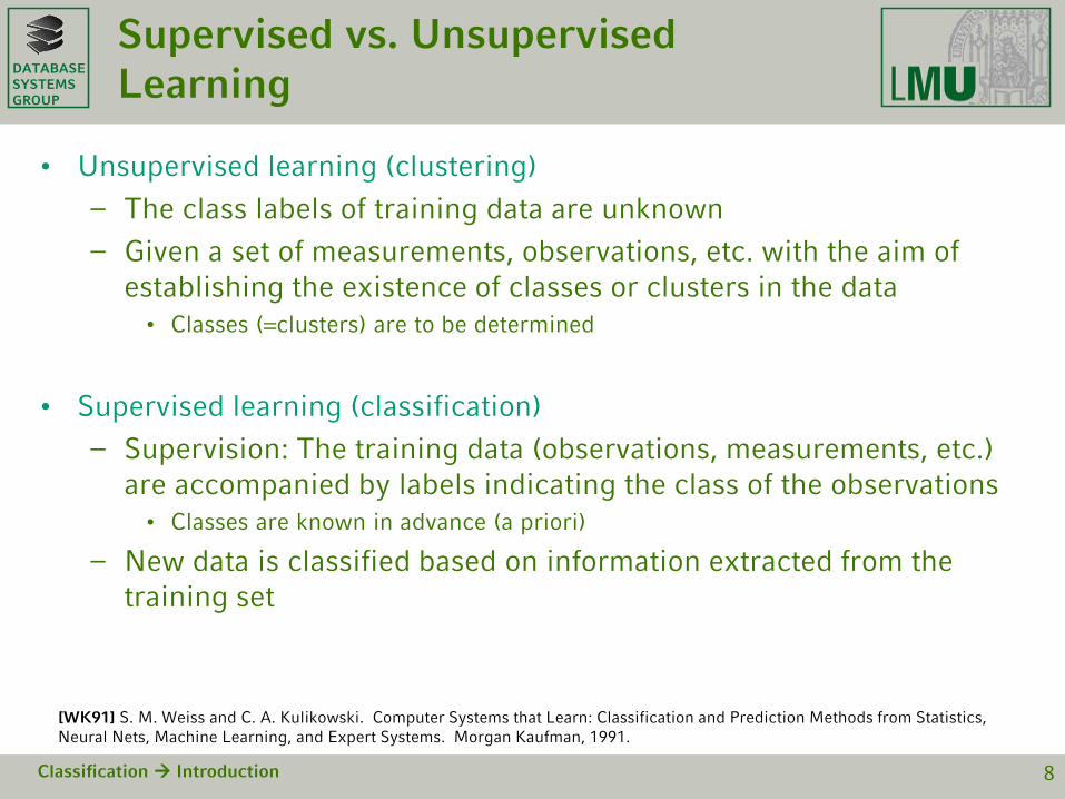
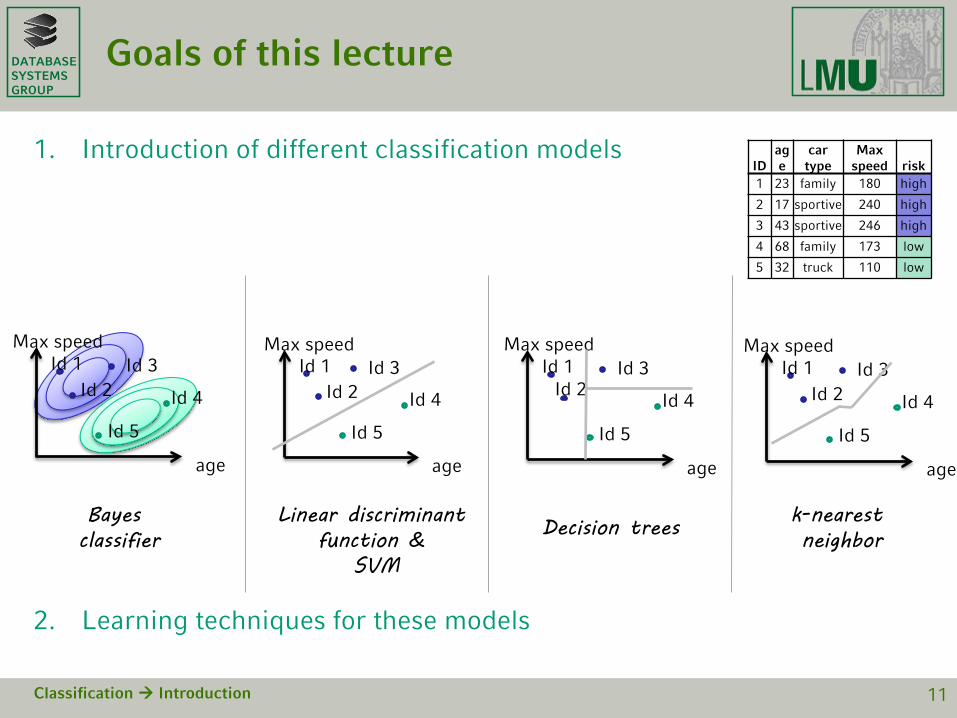
1. Introduction of different classification models
2. Learning techniques for these models
Classification Introduction 11
IDage
car type
Max speed risk
1 23 family 180 high
2 17 sportive 240 high
3 43 sportive 246 high
4 68 family 173 low
5 32 truck 110 low
age
Max speedId 1
Id 2Id 3
Id 5
Id 4
age
Max speedId 1
Id 2Id 3
Id 5
Id 4
age
Max speedId 1
Id 2Id 3
Id 5
Id 4
Linear discriminant function &
SVM
Decision trees k-nearest neighbor
Bayes classifier
age
Max speedId 1
Id 2Id 3
Id 5
Id 4

DATABASESYSTEMSGROUP
Quality Measures for Classifiers
• Classification accuracy or classification error (complementary)• Compactness of the model
– decision tree size; number of decision rules
• Interpretability of the model– Insights and understanding of the data provided by the model
• Efficiency– Time to generate the model (training time)
– Time to apply the model (prediction time)
• Scalability for large databases– Efficiency in disk-resident databases
• Robustness– Robust against noise or missing values
Classification Introduction 16
DATABASESYSTEMSGROUP
Evaluation of Classifiers – Notions
• Using training data to build a classifier and to estimate the model’s accuracy may result in misleading and overoptimistic estimates – due to overspecialization of the learning model to the training data
• Train-and-Test: Decomposition of labeled data set 𝑂𝑂 into two partitions– Training data is used to train the classifier
• construction of the model by using information about the class labels
– Test data is used to evaluate the classifier• temporarily hide class labels, predict them anew and compare results
with original class labels
• Train-and-Test is not applicable if the set of objects for which the class label is known is very small
Classification Introduction 17
DATABASESYSTEMSGROUP
Evaluation of Classifiers –Cross Validation
• m-fold Cross Validation– Decompose data set evenly into m subsets of (nearly) equal size
– Iteratively use m – 1 partitions as training data and the remaining single partition as test data.
– Combine the m classification accuracy values to an overall classification accuracy, and combine the m generated models to an overall model for the data.
• Leave-one-out is a special case of cross validation (m=n)– For each of the objects 𝑜𝑜 in the data set 𝑂𝑂:
• Use set 𝑂𝑂\{𝑜𝑜} as training set
• Use the singleton set {𝑜𝑜} as test set
– Compute classification accuracy by dividing the number of correct predictions through the database size 𝑂𝑂
– Particularly well applicable to nearest-neighbor classifiers
Classification Introduction 18
DATABASESYSTEMSGROUP
Quality Measures: Accuracy and Error
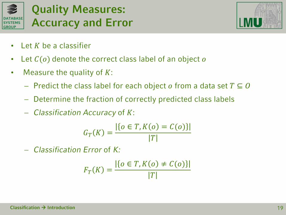
• Let 𝐾𝐾 be a classifier
• Let 𝐶𝐶(𝑜𝑜) denote the correct class label of an object 𝑜𝑜
• Measure the quality of 𝐾𝐾:
− Predict the class label for each object 𝑜𝑜 from a data set 𝑇𝑇 ⊆ 𝑂𝑂
− Determine the fraction of correctly predicted class labels
− Classification Accuracy of 𝐾𝐾:
𝐺𝐺𝑇𝑇 𝐾𝐾 =𝑜𝑜 ∈ 𝑇𝑇,𝐾𝐾 𝑜𝑜 = 𝐶𝐶(𝑜𝑜)
𝑇𝑇− Classification Error of K:
𝐹𝐹𝑇𝑇 𝐾𝐾 =𝑜𝑜 ∈ 𝑇𝑇,𝐾𝐾 𝑜𝑜 ≠ 𝐶𝐶(𝑜𝑜)
𝑇𝑇
Classification Introduction 19
DATABASESYSTEMSGROUP
Quality Measures: Accuracy and Error
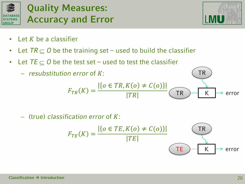
• Let 𝐾𝐾 be a classifier
• Let TR ⊆ O be the training set – used to build the classifier
• Let TE ⊆ O be the test set – used to test the classifier
− resubstitution error of 𝐾𝐾:
𝐹𝐹𝑇𝑇𝑇𝑇 𝐾𝐾 =𝑜𝑜 ∈ 𝑇𝑇𝑇𝑇,𝐾𝐾 𝑜𝑜 ≠ 𝐶𝐶(𝑜𝑜)
𝑇𝑇𝑇𝑇
− (true) classification error of 𝐾𝐾:
𝐹𝐹𝑇𝑇𝐸𝐸 𝐾𝐾 =𝑜𝑜 ∈ 𝑇𝑇𝑇𝑇,𝐾𝐾 𝑜𝑜 ≠ 𝐶𝐶(𝑜𝑜)
𝑇𝑇𝑇𝑇
Classification Introduction 20
TR
TR K error
TR
TE K error
DATABASESYSTEMSGROUP
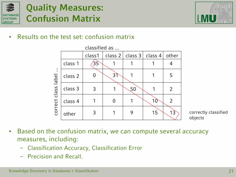
Quality Measures: Confusion Matrix
• Results on the test set: confusion matrix
• Based on the confusion matrix, we can compute several accuracymeasures, including:– Classification Accuracy, Classification Error
– Precision and Recall.
21
class1 class 2 class 3 class 4 other
class 1
class 2
class 3
class 4
other
35 1 1
0
3
1
3
31
1
1
50
10
1 9
1 4
1
1
5
2
210
15 13
classified as ...
corr
ect
clas
sla
bel.
..
correctly classifiedobjects
Knowledge Discovery in Databases I: Klassifikation
DATABASESYSTEMSGROUP
23
Quality Measures: Precision and Recall
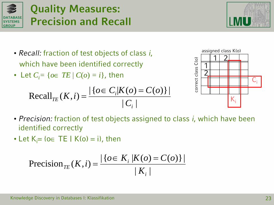
|||)}()(|{|),(Precision
i
iTE K
oCoKKoiK =∈=
Knowledge Discovery in Databases I: Klassifikation
•Recall: fraction of test objects of class i, which have been identified correctly
• Let Ci= {o∈ TE | C(o) = i}, then
•Precision: fraction of test objects assigned to class i, which have beenidentified correctly
•Let Ki= {o∈ TE | K(o) = i}, then
|||)}()(|{|),(Recall
i
iTE C
oCoKCoiK =∈=
Ci
Ki
assigned class K(o)
corr
ect
clas
sC
(o) 1 2
12
DATABASESYSTEMSGROUP
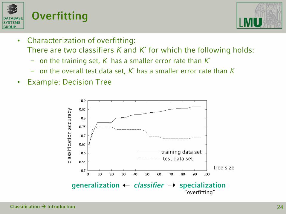
Overfitting
• Characterization of overfitting:There are two classifiers K and K´ for which the following holds:– on the training set, K has a smaller error rate than K´
– on the overall test data set, K´ has a smaller error rate than K
• Example: Decision Tree
Classification Introduction 24
clas
sifi
cati
on a
ccur
acy
generalization classifier specialization
training data settest data set
“overfitting”
tree size
DATABASESYSTEMSGROUP
Overfitting (2)
• Overfitting– occurs when the classifier is too optimized to the (noisy) training data
– As a result, the classifier yields worse results on the test data set
– Potential reasons• bad quality of training data (noise, missing values, wrong values)
• different statistical characteristics of training data and test data
• Overfitting avoidance– Removal of noisy and erroneous training data; in particular,
remove contradicting training data
– Choice of an appropriate size of the training set: not too small, not too large
– Choice of appropriate sample: sample should describe all aspects of the domain and not only parts of it
Classification Introduction 25

DATABASESYSTEMSGROUP
Underfitting
• Underfitting– Occurs when the classifiers model is too simple, e.g. trying to separate
classes linearly that can only be separated by a quadratic surface
– happens seldomly
• Trade-off – Usually one has to find a good balance between over- and underfitting
Classification Introduction 26
DATABASESYSTEMSGROUP
Chapter 6: Classification
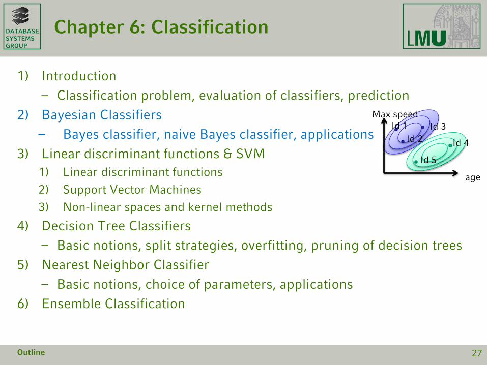
1) Introduction– Classification problem, evaluation of classifiers, prediction
2) Bayesian Classifiers– Bayes classifier, naive Bayes classifier, applications
3) Linear discriminant functions & SVM1) Linear discriminant functions
2) Support Vector Machines
3) Non-linear spaces and kernel methods
4) Decision Tree Classifiers– Basic notions, split strategies, overfitting, pruning of decision trees
5) Nearest Neighbor Classifier– Basic notions, choice of parameters, applications
6) Ensemble Classification
Outline 27
age
Max speedId 1
Id 2Id 3
Id 5
Id 4
DATABASESYSTEMSGROUP
Bayes Classification
• Probability based classification– Based on likelihood of observed data, estimate explicit probabilities for
classes
– Classify objects depending on costs for possible decisions and the probabilities for the classes
• Incremental– Likelihood functions built up from classified data
– Each training example can incrementally increase/decrease the probability that a hypothesis (class) is correct
– Prior knowledge can be combined with observed data.
• Good classification results in many applications
Classification Bayesian Classifiers 28
DATABASESYSTEMSGROUP
Bayes’ theorem
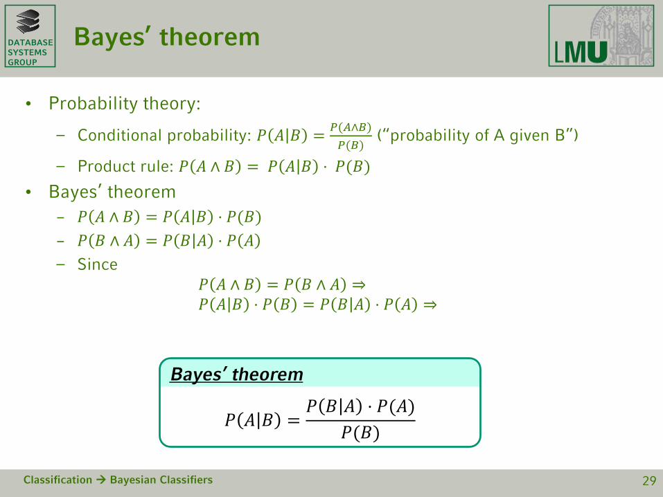
• Probability theory:
– Conditional probability: 𝑃𝑃 𝐴𝐴 𝐵𝐵 = 𝑃𝑃(𝐴𝐴∧𝐵𝐵)𝑃𝑃(𝐵𝐵)
(“probability of A given B”)
– Product rule: 𝑃𝑃 𝐴𝐴 ∧ 𝐵𝐵 = 𝑃𝑃 𝐴𝐴 𝐵𝐵 ⋅ 𝑃𝑃(𝐵𝐵)• Bayes’ theorem
– 𝑃𝑃 𝐴𝐴 ∧ 𝐵𝐵 = 𝑃𝑃 𝐴𝐴 𝐵𝐵 ⋅ 𝑃𝑃(𝐵𝐵)– 𝑃𝑃 𝐵𝐵 ∧ 𝐴𝐴 = 𝑃𝑃 𝐵𝐵 𝐴𝐴 ⋅ 𝑃𝑃 𝐴𝐴– Since
𝑃𝑃 𝐴𝐴 ∧ 𝐵𝐵 = 𝑃𝑃 𝐵𝐵 ∧ 𝐴𝐴 ⇒𝑃𝑃 𝐴𝐴 𝐵𝐵 ⋅ 𝑃𝑃 𝐵𝐵 = 𝑃𝑃 𝐵𝐵 𝐴𝐴 ⋅ 𝑃𝑃 𝐴𝐴 ⇒
Classification Bayesian Classifiers 29
Bayes’ theorem
𝑃𝑃 𝐴𝐴 𝐵𝐵 =𝑃𝑃 𝐵𝐵 𝐴𝐴 ⋅ 𝑃𝑃(𝐴𝐴)
𝑃𝑃(𝐵𝐵)
DATABASESYSTEMSGROUP
Bayes Classifier
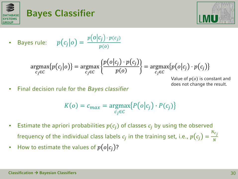
• Bayes rule: 𝑝𝑝 𝑐𝑐𝑗𝑗 𝑜𝑜 =𝑝𝑝 𝑜𝑜 𝑐𝑐𝑗𝑗 � 𝑝𝑝(𝑐𝑐𝑗𝑗)
𝑝𝑝(𝑜𝑜)
argmax𝑐𝑐𝑗𝑗∈𝐶𝐶
𝑝𝑝 𝑐𝑐𝑗𝑗 𝑜𝑜 = argmax𝑐𝑐𝑗𝑗∈𝐶𝐶
𝑝𝑝 𝑜𝑜 𝑐𝑐𝑗𝑗 ⋅ 𝑝𝑝 𝑐𝑐𝑗𝑗𝑝𝑝 𝑜𝑜
= argmax𝑐𝑐𝑗𝑗∈𝐶𝐶
𝑝𝑝 𝑜𝑜 𝑐𝑐𝑗𝑗 ⋅ 𝑝𝑝 𝑐𝑐𝑗𝑗
• Final decision rule for the Bayes classifier
𝐾𝐾 𝑜𝑜 = 𝑐𝑐𝑚𝑚𝑚𝑚𝑚𝑚 = argmax𝑐𝑐𝑗𝑗∈𝐶𝐶
𝑃𝑃 𝑜𝑜 𝑐𝑐𝑗𝑗 � 𝑃𝑃(𝑐𝑐𝑗𝑗)
• Estimate the apriori probabilities 𝑝𝑝(𝑐𝑐𝑗𝑗) of classes 𝑐𝑐𝑗𝑗 by using the observed
frequency of the individual class labels 𝑐𝑐𝑗𝑗 in the training set, i.e., 𝑝𝑝 𝑐𝑐𝑗𝑗 =𝑁𝑁𝑐𝑐𝑗𝑗𝑁𝑁
• How to estimate the values of 𝑝𝑝 𝑜𝑜 𝑐𝑐𝑗𝑗 ?
Classification Bayesian Classifiers 30
Value of 𝑝𝑝(𝑜𝑜) is constant and does not change the result.

DATABASESYSTEMSGROUP
Density estimation techniques
• Given a database DB, how to estimate conditional probability 𝑝𝑝 𝑜𝑜 𝑐𝑐𝑗𝑗 ?– Parametric methods: e.g. single Gaussian distribution
• Compute by maximum likelihood estimators (MLE), etc.
– Non-parametric methods: Kernel methods• Parzen’s window, Gaussian kernels, etc.
– Mixture models: e.g. mixture of Gaussians (GMM = Gaussian Mixture Model)• Compute by e.g. EM algorithm
• Curse of dimensionality often lead to problems in high dimensional data– Density functions become too uninformative
– Solution:• Dimensionality reduction
• Usage of statistical independence of single attributes (extreme case: naïve Bayes)
Classification Bayesian Classifiers 31
DATABASESYSTEMSGROUP
Naïve Bayes Classifier (1)
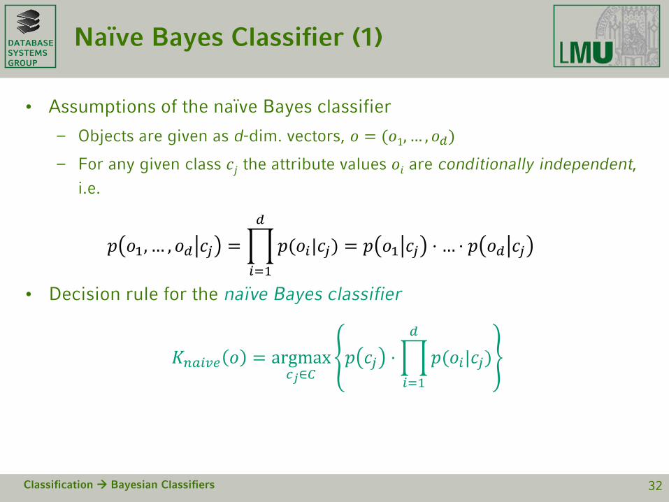
• Assumptions of the naïve Bayes classifier
– Objects are given as d-dim. vectors, 𝑜𝑜 = (𝑜𝑜1, … , 𝑜𝑜𝑑𝑑)
– For any given class 𝑐𝑐𝑗𝑗 the attribute values 𝑜𝑜𝑖𝑖 are conditionally independent, i.e.
𝑝𝑝 𝑜𝑜1, … , 𝑜𝑜𝑑𝑑 𝑐𝑐𝑗𝑗 = �𝑖𝑖=1
𝑑𝑑
𝑝𝑝(𝑜𝑜𝑖𝑖|𝑐𝑐𝑗𝑗) = 𝑝𝑝 𝑜𝑜1 𝑐𝑐𝑗𝑗 ⋅ … ⋅ 𝑝𝑝 𝑜𝑜𝑑𝑑 𝑐𝑐𝑗𝑗
• Decision rule for the naïve Bayes classifier
𝐾𝐾𝑛𝑛𝑚𝑚𝑖𝑖𝑛𝑛𝑛𝑛 𝑜𝑜 = argmax𝑐𝑐𝑗𝑗∈𝐶𝐶
𝑝𝑝 𝑐𝑐𝑗𝑗 ⋅�𝑖𝑖=1
𝑑𝑑
𝑝𝑝(𝑜𝑜𝑖𝑖|𝑐𝑐𝑗𝑗)
Classification Bayesian Classifiers 32

DATABASESYSTEMSGROUP
Naïve Bayes Classifier (2)
• Independency assumption: 𝑝𝑝 𝑜𝑜1, … , 𝑜𝑜𝑑𝑑 𝑐𝑐𝑗𝑗 = ∏𝑖𝑖=1𝑑𝑑 𝑝𝑝(𝑜𝑜𝑖𝑖|𝑐𝑐𝑗𝑗)
• If i-th attribute is categorical:𝑝𝑝(𝑜𝑜𝑖𝑖|𝐶𝐶) can be estimated as the relative frequencyof samples having value 𝑥𝑥𝑖𝑖 as 𝑖𝑖-th attribute in class C in the training set
• If i-th attribute is continuous:𝑝𝑝 𝑜𝑜𝑖𝑖 𝐶𝐶 can, for example, be estimated through:– Gaussian density function determined by (µ𝑖𝑖,𝑗𝑗 ,σ𝑖𝑖,𝑗𝑗)
𝑝𝑝 𝑜𝑜𝑖𝑖 𝐶𝐶𝑗𝑗 = 12𝜋𝜋𝜎𝜎𝑖𝑖,𝑗𝑗
e−12
𝑜𝑜𝑖𝑖−𝜇𝜇𝑖𝑖,𝑗𝑗𝜎𝜎𝑖𝑖,𝑗𝑗
2
• Computationally easy in both cases
Classification Bayesian Classifiers 33
p(oi|C3)
xiµi,3
p(oi|C2)
xiµi,2
p(oi|C1)
xiµi,1
xi
p(oi|Cj)
f(xi)
q
DATABASESYSTEMSGROUP
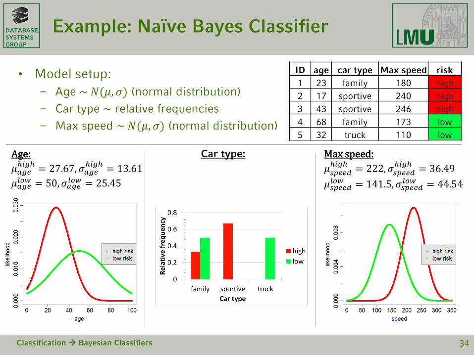
Example: Naïve Bayes Classifier
• Model setup:– Age ~ 𝑁𝑁(𝜇𝜇,𝜎𝜎) (normal distribution)
– Car type ~ relative frequencies
– Max speed ~ 𝑁𝑁(𝜇𝜇,𝜎𝜎) (normal distribution)
Classification Bayesian Classifiers 34
ID age car type Max speed risk1 23 family 180 high2 17 sportive 240 high3 43 sportive 246 high4 68 family 173 low5 32 truck 110 low
Max speed:𝜇𝜇𝑠𝑠𝑝𝑝𝑛𝑛𝑛𝑛𝑑𝑑ℎ𝑖𝑖𝑖𝑖ℎ = 222,𝜎𝜎𝑠𝑠𝑝𝑝𝑛𝑛𝑛𝑛𝑑𝑑
ℎ𝑖𝑖𝑖𝑖ℎ = 36.49𝜇𝜇𝑠𝑠𝑝𝑝𝑛𝑛𝑛𝑛𝑑𝑑𝑙𝑙𝑜𝑜𝑙𝑙 = 141.5,𝜎𝜎𝑠𝑠𝑝𝑝𝑛𝑛𝑛𝑛𝑑𝑑𝑙𝑙𝑜𝑜𝑙𝑙 = 44.54
Age:𝜇𝜇𝑚𝑚𝑖𝑖𝑛𝑛ℎ𝑖𝑖𝑖𝑖ℎ = 27.67,𝜎𝜎𝑚𝑚𝑖𝑖𝑛𝑛
ℎ𝑖𝑖𝑖𝑖ℎ = 13.61𝜇𝜇𝑚𝑚𝑖𝑖𝑛𝑛𝑙𝑙𝑜𝑜𝑙𝑙 = 50,𝜎𝜎𝑚𝑚𝑖𝑖𝑛𝑛𝑙𝑙𝑜𝑜𝑙𝑙 = 25.45
Car type:
DATABASESYSTEMSGROUP
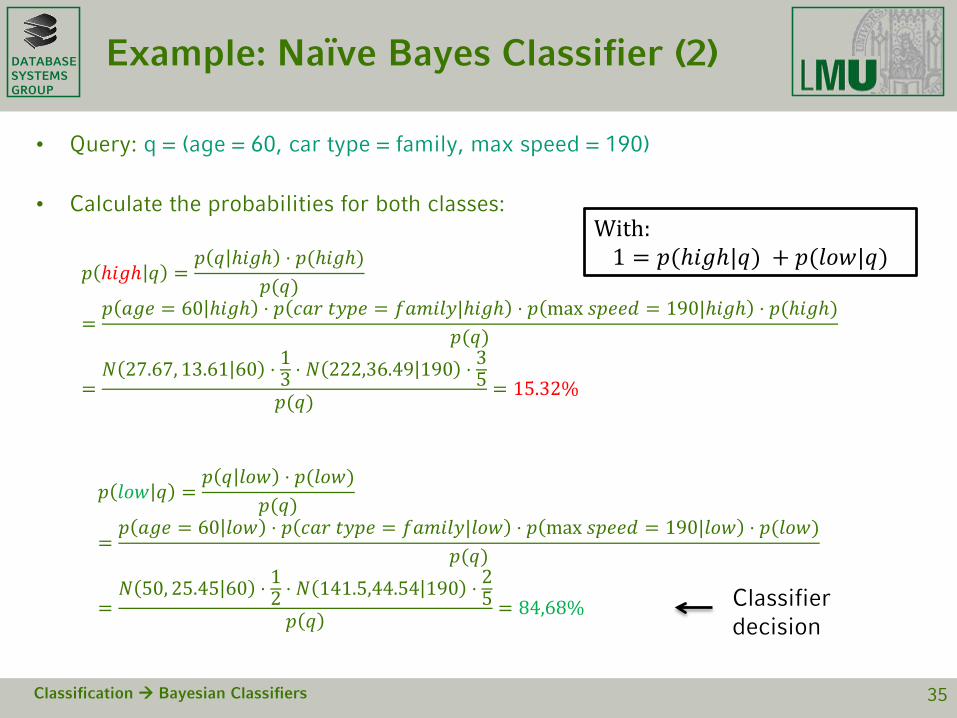
Example: Naïve Bayes Classifier (2)
• Query: q = (age = 60, car type = family, max speed = 190)
• Calculate the probabilities for both classes:
𝑝𝑝 ℎ𝑖𝑖𝑖𝑖ℎ 𝑞𝑞 =𝑝𝑝 𝑞𝑞 ℎ𝑖𝑖𝑖𝑖ℎ ⋅ 𝑝𝑝(ℎ𝑖𝑖𝑖𝑖ℎ)
𝑝𝑝(𝑞𝑞)
=𝑝𝑝 𝑎𝑎𝑖𝑖𝑎𝑎 = 60 ℎ𝑖𝑖𝑖𝑖ℎ ⋅ 𝑝𝑝 𝑐𝑐𝑎𝑎𝑐𝑐 𝑡𝑡𝑦𝑦𝑝𝑝𝑎𝑎 = 𝑓𝑓𝑎𝑎𝑓𝑓𝑖𝑖𝑓𝑓𝑦𝑦|ℎ𝑖𝑖𝑖𝑖ℎ ⋅ 𝑝𝑝 max 𝑠𝑠𝑝𝑝𝑎𝑎𝑎𝑎𝑑𝑑 = 190|ℎ𝑖𝑖𝑖𝑖ℎ ⋅ 𝑝𝑝(ℎ𝑖𝑖𝑖𝑖ℎ)
𝑝𝑝(𝑞𝑞)
=𝑁𝑁 27.67, 13.61 60 ⋅ 1
3 ⋅ 𝑁𝑁 222,36.49 190 ⋅ 35
𝑝𝑝(𝑞𝑞)= 15.32%
𝑝𝑝 𝑓𝑓𝑜𝑜𝑙𝑙 𝑞𝑞 =𝑝𝑝 𝑞𝑞 𝑓𝑓𝑜𝑜𝑙𝑙 ⋅ 𝑝𝑝(𝑓𝑓𝑜𝑜𝑙𝑙)
𝑝𝑝(𝑞𝑞)
=𝑝𝑝 𝑎𝑎𝑖𝑖𝑎𝑎 = 60 𝑓𝑓𝑜𝑜𝑙𝑙 ⋅ 𝑝𝑝 𝑐𝑐𝑎𝑎𝑐𝑐 𝑡𝑡𝑦𝑦𝑝𝑝𝑎𝑎 = 𝑓𝑓𝑎𝑎𝑓𝑓𝑖𝑖𝑓𝑓𝑦𝑦|𝑓𝑓𝑜𝑜𝑙𝑙 ⋅ 𝑝𝑝 max 𝑠𝑠𝑝𝑝𝑎𝑎𝑎𝑎𝑑𝑑 = 190|𝑓𝑓𝑜𝑜𝑙𝑙 ⋅ 𝑝𝑝(𝑓𝑓𝑜𝑜𝑙𝑙)
𝑝𝑝(𝑞𝑞)
=𝑁𝑁 50, 25.45 60 ⋅ 1
2 ⋅ 𝑁𝑁 141.5,44.54 190 ⋅ 25
𝑝𝑝 𝑞𝑞= 84,68%
Classification Bayesian Classifiers 35
With:1 = 𝑝𝑝(ℎ𝑖𝑖𝑖𝑖ℎ|𝑞𝑞) + 𝑝𝑝(𝑓𝑓𝑜𝑜𝑙𝑙|𝑞𝑞)
Classifier decision

DATABASESYSTEMSGROUP
Bayesian Classifier
• Assuming dimensions of o =(o1…od ) are not independent• Assume multivariate normal distribution (=Gaussian)
with
𝜇𝜇𝑗𝑗 mean vector of class 𝐶𝐶𝑗𝑗𝑁𝑁𝑗𝑗 is number of objects of class 𝐶𝐶𝑗𝑗Σ𝑗𝑗 is the 𝑑𝑑 × 𝑑𝑑 covariance matrix
Σ𝑗𝑗 = 1𝑁𝑁𝑗𝑗−1
∑𝑖𝑖=1𝑁𝑁𝑗𝑗 𝑜𝑜𝑖𝑖 − 𝜇𝜇𝑗𝑗
𝑇𝑇 ⋅ 𝑜𝑜𝑖𝑖 − 𝜇𝜇𝑗𝑗
|Σ𝑗𝑗| is the determinant of Σ𝑗𝑗 and Σ𝑗𝑗−1 the inverse of Σ𝑗𝑗
Classification Bayesian Classifiers 36
( )T
jjj oo
jdj e)CP(o
)()(21
2/12/
1
||21|
µµ
π−Σ−− −
Σ=
(outer product)

DATABASESYSTEMSGROUP
Example: Interpretation of Raster Images
• Scenario: automated interpretation of raster images– Take an image from a certain region (in d different frequency bands, e.g.,
infrared, etc.)
– Represent each pixel by d values: (o1, …, od)
• Basic assumption: different surface properties of the earth („landuse“) follow a characteristic reflection and emission pattern
Classification Bayesian Classifiers 37
• • • •• • • •• • • •• • • •
• • • •• • • •• • • •• • • •
Surface of the earth Feature-space
Band 1
Band 216.5 22.020.018.08
12
10
•
(12),(17.5)
••••
••• •
••
••••1 1 1 21 1 2 23 2 3 23 3 3 3
FarmlandWater
town
(8.5),(18.7)

DATABASESYSTEMSGROUP
Example: Interpretation of Raster Images
• Application of the Bayes classifier– Estimation of the p(o | c) without assumption of conditional independence
– Assumption of d-dimensional normal (= Gaussian) distributions for the value vectors of a class
Classification Bayesian Classifiers 38
farmland
townwater
decision regions
Probability p ofclass membership
DATABASESYSTEMSGROUP
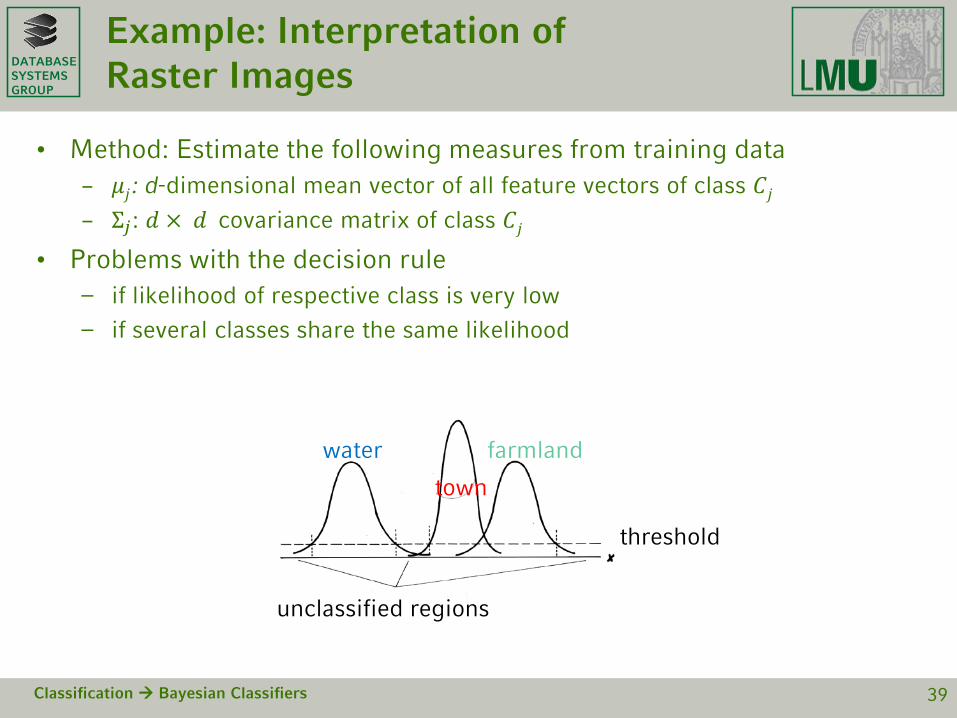
Example: Interpretation of Raster Images
• Method: Estimate the following measures from training data– 𝜇𝜇𝑗𝑗: d-dimensional mean vector of all feature vectors of class 𝐶𝐶𝑗𝑗– Σ𝑗𝑗: 𝑑𝑑 × 𝑑𝑑 covariance matrix of class 𝐶𝐶𝑗𝑗
• Problems with the decision rule– if likelihood of respective class is very low
– if several classes share the same likelihood
Classification Bayesian Classifiers 39
unclassified regions
threshold
water
town
farmland

DATABASESYSTEMSGROUP
Bayesian Classifiers – Discussion
• Pro– High classification accuracy for many applications if density function
defined properly
– Incremental computation many models can be adopted to new training objects by updating densities • For Gaussian: store count, sum, squared sum to derive mean, variance• For histogram: store count to derive relative frequencies
– Incorporation of expert knowledge about the application in the prior 𝑃𝑃 𝐶𝐶𝑖𝑖
• Contra– Limited applicability often, required conditional probabilities are not available
– Lack of efficient computation in case of a high number of attributes particularly for Bayesian belief networks
Classification Bayesian Classifiers 40
DATABASESYSTEMSGROUP
The independence hypothesis…
• … makes efficient computation possible• … yields optimal classifiers when satisfied• … but is seldom satisfied in practice, as attributes (variables) are often
correlated.• Attempts to overcome this limitation:
– Bayesian networks, that combine Bayesian reasoning with causal relationships between attributes
– Decision trees, that reason on one attribute at the time, considering most important attributes first
Classification Bayesian Classifiers 41

DATABASESYSTEMSGROUP
Chapter 6: Classification
1) Introduction– Classification problem, evaluation of classifiers, prediction
2) Bayesian Classifiers– Bayes classifier, naive Bayes classifier, applications
3) Linear discriminant functions & SVM1) Linear discriminant functions
2) Support Vector Machines
3) Non-linear spaces and kernel methods
4) Decision Tree Classifiers– Basic notions, split strategies, overfitting, pruning of decision trees
5) Nearest Neighbor Classifier– Basic notions, choice of parameters, applications
6) Ensemble Classification
Outline 42
age
Max speedId 1
Id 2Id 3
Id 5
Id 4
DATABASESYSTEMSGROUP
Linear discriminant function classifier
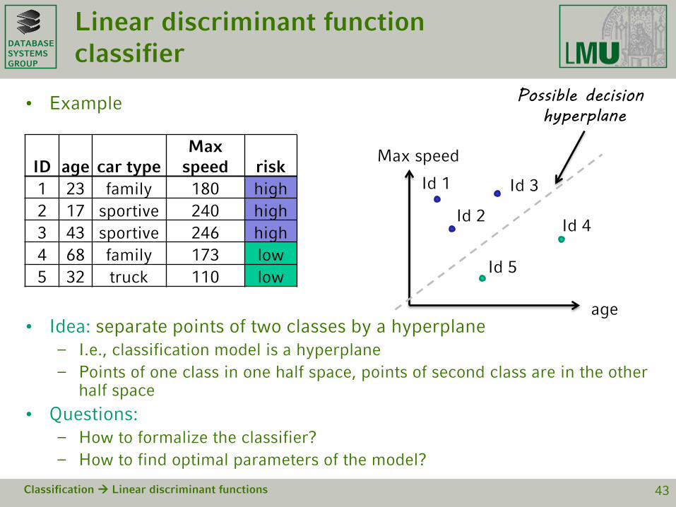
• Example
• Idea: separate points of two classes by a hyperplane– I.e., classification model is a hyperplane – Points of one class in one half space, points of second class are in the other
half space
• Questions: – How to formalize the classifier?– How to find optimal parameters of the model?
Classification Linear discriminant functions 43
ID age car typeMax
speed risk1 23 family 180 high2 17 sportive 240 high3 43 sportive 246 high4 68 family 173 low5 32 truck 110 low
age
Max speed
Id 1
Id 2
Id 3
Id 5
Id 4
Possible decision hyperplane

DATABASESYSTEMSGROUP
Basic notions
• Recall some general algebraic notions for a vector space 𝑉𝑉:– 𝐱𝐱, 𝐲𝐲 denotes an inner product of two vectors 𝐱𝐱, 𝐲𝐲 ∈ 𝑉𝑉:
e.g., the scalar product: 𝐱𝐱, 𝐲𝐲 = 𝐱𝐱𝑇𝑇𝐲𝐲 = ∑𝑖𝑖=1𝑑𝑑 (x𝑖𝑖 ⋅ y𝑖𝑖)
– 𝐻𝐻 𝐰𝐰,𝑙𝑙0 denotes a hyperplane with normal vector w and constant term 𝑙𝑙0:𝐱𝐱 ∈ 𝐻𝐻 𝐰𝐰,𝑙𝑙0 ⇔ 𝐰𝐰, 𝐱𝐱 + 𝑙𝑙0 = 0
– The normal vector w may be normalized to 𝒘𝒘𝒘:
𝐰𝐰′ =1𝐰𝐰,𝐰𝐰
⋅ 𝐰𝐰 ⟹ 𝐰𝐰′,𝐰𝐰′ = 1
– Distance of a vector x to the hyperplane 𝐻𝐻(𝐰𝐰𝒘,𝑙𝑙0):𝑑𝑑𝑖𝑖𝑠𝑠𝑡𝑡 𝐱𝐱,𝐻𝐻 𝐰𝐰𝒘,𝑙𝑙0 = 𝐰𝐰𝒘, 𝐱𝐱 + 𝑙𝑙0
Classification Linear discriminant functions 44

DATABASESYSTEMSGROUP
Formalization
• Consider a two-class example (generalizations later on):– 𝐷𝐷: d-dimensional vector space with attributes 𝑎𝑎𝑖𝑖, 𝑖𝑖 = 1, … ,𝑑𝑑– 𝑌𝑌 = −1, 1 set of 2 distinct class labels 𝑦𝑦𝑗𝑗– 𝑂𝑂 ⊆ 𝐷𝐷: set of objects, 𝐨𝐨 = (𝑜𝑜1, … , 𝑜𝑜𝑑𝑑), with known class labels 𝑦𝑦 ∈ 𝑌𝑌 and
cardinality of 𝑂𝑂 = 𝑁𝑁
• A hyperplane 𝐻𝐻 𝐰𝐰,𝑙𝑙0 with normal vector 𝐰𝐰 and constant term 𝑙𝑙0𝐱𝐱 ∈ 𝐻𝐻 ⇔ 𝐰𝐰𝑇𝑇𝐱𝐱 + 𝑙𝑙0 = 0
• Classification rule (linear classifier) given by:
Classification Linear discriminant functions 45
𝐰𝐰𝑇𝑇𝐱𝐱 + 𝑙𝑙0 = 0
𝐰𝐰𝑇𝑇𝐱𝐱 + 𝑙𝑙0 > 0𝐰𝐰𝑇𝑇𝐱𝐱 + 𝑙𝑙0 < 0
Classification rule
𝐾𝐾𝐻𝐻(𝐰𝐰,𝑙𝑙0) 𝐱𝐱 = sign 𝐰𝐰𝑇𝑇𝐱𝐱 + 𝑙𝑙0
DATABASESYSTEMSGROUP
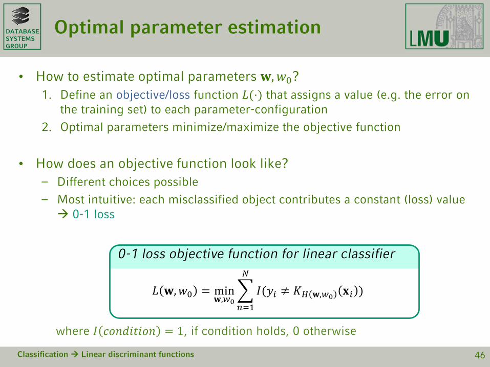
Optimal parameter estimation
• How to estimate optimal parameters 𝐰𝐰,𝑙𝑙0?1. Define an objective/loss function 𝐿𝐿(⋅) that assigns a value (e.g. the error on
the training set) to each parameter-configuration
2. Optimal parameters minimize/maximize the objective function
• How does an objective function look like?– Different choices possible
– Most intuitive: each misclassified object contributes a constant (loss) value 0-1 loss
Classification Linear discriminant functions 46
0-1 loss objective function for linear classifier
𝐿𝐿 𝐰𝐰,𝑙𝑙0 = min𝐰𝐰,𝑙𝑙0
�𝑛𝑛=1
𝑁𝑁
𝐼𝐼(𝑦𝑦𝑖𝑖 ≠ 𝐾𝐾𝐻𝐻 𝐰𝐰,𝑙𝑙0 𝐱𝐱𝑖𝑖 )
where 𝐼𝐼 𝑐𝑐𝑜𝑜𝑐𝑐𝑑𝑑𝑖𝑖𝑡𝑡𝑖𝑖𝑜𝑜𝑐𝑐 = 1, if condition holds, 0 otherwise
DATABASESYSTEMSGROUP
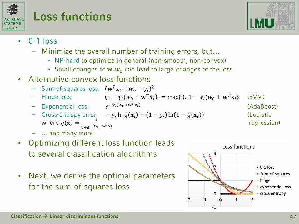
Loss functions
• 0-1 loss– Minimize the overall number of training errors, but…
• NP-hard to optimize in general (non-smooth, non-convex)• Small changes of 𝐰𝐰,𝑙𝑙0 can lead to large changes of the loss
• Alternative convex loss functions– Sum-of-squares loss: 𝐰𝐰𝑇𝑇𝐱𝐱𝑖𝑖 + 𝑙𝑙0 − 𝑦𝑦𝑖𝑖 2
– Hinge loss: 1 − 𝑦𝑦𝑖𝑖(𝑙𝑙0 + 𝐰𝐰𝑇𝑇𝐱𝐱𝑖𝑖 += max{0, 1 − 𝑦𝑦𝑖𝑖(𝑙𝑙0 + 𝐰𝐰𝑇𝑇𝐱𝐱𝑖𝑖} (SVM)
– Exponential loss: 𝑎𝑎−𝑦𝑦𝑖𝑖(𝑙𝑙0+𝐰𝐰𝑇𝑇𝐱𝐱𝑖𝑖) (AdaBoost)– Cross-entropy error: −𝑦𝑦𝑖𝑖 ln𝑖𝑖 𝐱𝐱𝑖𝑖 + 1 − 𝑦𝑦𝑖𝑖 ln 1 − 𝑖𝑖(𝐱𝐱𝑖𝑖) (Logistic
where 𝑖𝑖 𝐱𝐱 = 11+𝑛𝑛−(𝑤𝑤0+𝐰𝐰𝑇𝑇𝐱𝐱) regression)
– … and many more
• Optimizing different loss function leads to several classification algorithms
• Next, we derive the optimal parametersfor the sum-of-squares loss
Classification Linear discriminant functions 47

DATABASESYSTEMSGROUP
Optimal parameters for SSE loss
• Loss/Objective function: sum-of-squares error to real class values
• Minimize the error function for getting optimal parameters– Use standard optimization technique:
1. Calculate first derivative
2. Set derivative to zero and compute the global minimum (SSE is a convex function)
Classification Linear discriminant functions 48
Objective function
𝑆𝑆𝑆𝑆𝑇𝑇 𝐰𝐰,𝑙𝑙0 = �𝑖𝑖=1..𝑁𝑁
𝐰𝐰𝑇𝑇𝐱𝐱𝑖𝑖 + 𝑙𝑙0 − 𝑦𝑦𝑖𝑖 2
DATABASESYSTEMSGROUP
Optimal parameters for SSE loss (cont’d)
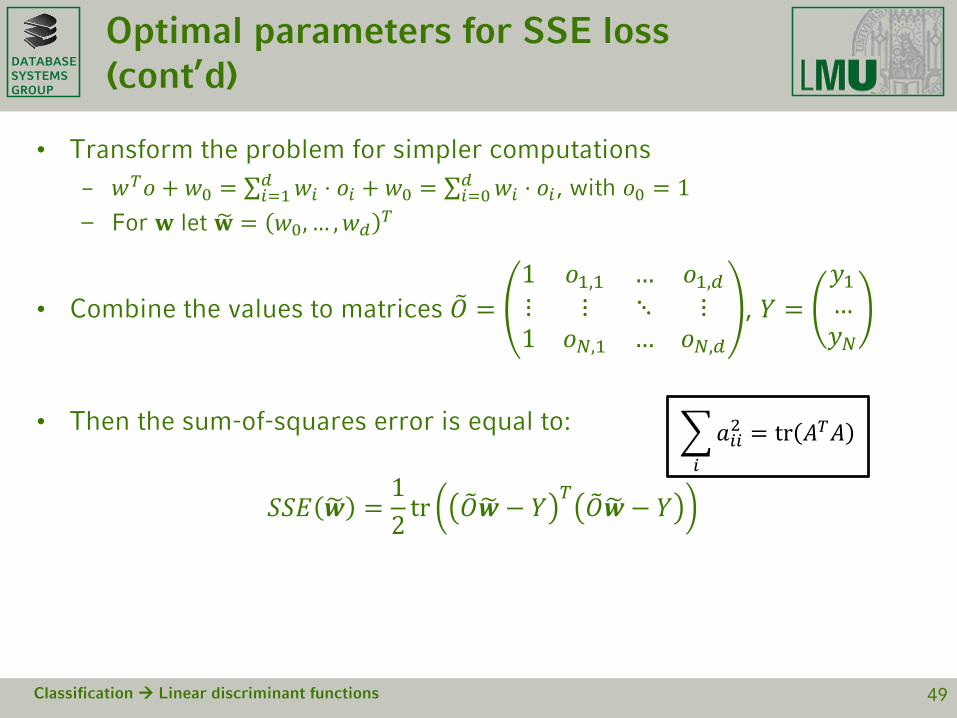
• Transform the problem for simpler computations– 𝑙𝑙𝑇𝑇𝑜𝑜 + 𝑙𝑙0 = ∑𝑖𝑖=1𝑑𝑑 𝑙𝑙𝑖𝑖 ⋅ 𝑜𝑜𝑖𝑖 + 𝑙𝑙0 = ∑𝑖𝑖=0𝑑𝑑 𝑙𝑙𝑖𝑖 ⋅ 𝑜𝑜𝑖𝑖, with 𝑜𝑜0 = 1– For 𝐰𝐰 let �𝐰𝐰 = 𝑙𝑙0, … ,𝑙𝑙𝑑𝑑 𝑇𝑇
• Combine the values to matrices �𝑂𝑂 =1 𝑜𝑜1,1 … 𝑜𝑜1,𝑑𝑑⋮ ⋮ ⋱ ⋮1 𝑜𝑜𝑁𝑁,1 … 𝑜𝑜𝑁𝑁,𝑑𝑑
, 𝑌𝑌 =𝑦𝑦1…𝑦𝑦𝑁𝑁
• Then the sum-of-squares error is equal to:
𝑆𝑆𝑆𝑆𝑇𝑇 �𝒘𝒘 =12
tr �𝑂𝑂�𝒘𝒘− 𝑌𝑌 𝑇𝑇 �𝑂𝑂�𝒘𝒘− 𝑌𝑌
Classification Linear discriminant functions 49
�𝑖𝑖
𝑎𝑎𝑖𝑖𝑖𝑖2 = tr 𝐴𝐴𝑇𝑇𝐴𝐴
DATABASESYSTEMSGROUP
Optimal parameters for SSE loss (cont’d)
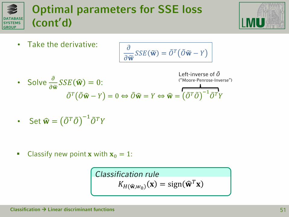
• Take the derivative:
• Solve 𝜕𝜕𝜕𝜕 �𝐰𝐰𝑆𝑆𝑆𝑆𝑇𝑇 �𝐰𝐰 = 0:
�𝑂𝑂𝑇𝑇 �𝑂𝑂 �𝐰𝐰 − 𝑌𝑌 = 0 ⇔ �𝑂𝑂 �𝐰𝐰 = 𝑌𝑌 ⇔ �𝐰𝐰 = �𝑂𝑂𝑇𝑇 �𝑂𝑂 −1 �𝑂𝑂𝑇𝑇𝑌𝑌
• Set �𝐰𝐰 = �𝑂𝑂𝑇𝑇 �𝑂𝑂 −1 �𝑂𝑂𝑇𝑇𝑌𝑌
Classify new point 𝐱𝐱 with 𝐱𝐱0 = 1:
Classification Linear discriminant functions 51
Left-inverse of �𝑂𝑂(“Moore-Penrose-Inverse”)
Classification rule𝐾𝐾𝐻𝐻(�𝐰𝐰,𝑙𝑙0) 𝐱𝐱 = sign �𝐰𝐰𝑇𝑇𝐱𝐱
𝜕𝜕𝜕𝜕 �𝐰𝐰
𝑆𝑆𝑆𝑆𝑇𝑇 �𝐰𝐰 = �𝑂𝑂𝑇𝑇 �𝑂𝑂 �𝐰𝐰− 𝑌𝑌
DATABASESYSTEMSGROUP
Example SSE
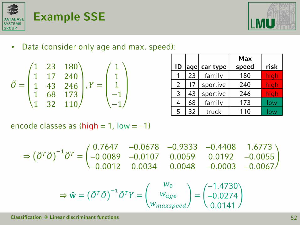
• Data (consider only age and max. speed):
�𝑂𝑂 =
1 23 1801 17 2401 43 2461 68 1731 32 110
,𝑌𝑌 =
111−1−1
encode classes as {high = 1, low = –1}
⇒ �𝑂𝑂𝑇𝑇 �𝑂𝑂 −1 �𝑂𝑂𝑇𝑇 =0.7647 −0.0678 −0.9333 −0.4408 1.6773−0.0089 −0.0107 0.0059 0.0192 −0.0055−0.0012 0.0034 0.0048 −0.0003 −0.0067
⇒ �𝐰𝐰 = �𝑂𝑂𝑇𝑇 �𝑂𝑂 −1 �𝑂𝑂𝑇𝑇𝑌𝑌 =𝑙𝑙0𝑙𝑙𝑚𝑚𝑖𝑖𝑛𝑛
𝑙𝑙𝑚𝑚𝑚𝑚𝑚𝑚𝑠𝑠𝑝𝑝𝑛𝑛𝑛𝑛𝑑𝑑=
−1.4730−0.02740.0141
Classification Linear discriminant functions 52
ID age car typeMax
speed risk1 23 family 180 high2 17 sportive 240 high3 43 sportive 246 high4 68 family 173 low5 32 truck 110 low
DATABASESYSTEMSGROUP
Example SSE (cont’d)
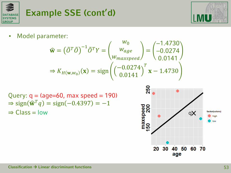
• Model parameter:
�𝐰𝐰 = �𝑂𝑂𝑇𝑇 �𝑂𝑂 −1 �𝑂𝑂𝑇𝑇𝑌𝑌 =𝑙𝑙0𝑙𝑙𝑚𝑚𝑖𝑖𝑛𝑛
𝑙𝑙𝑚𝑚𝑚𝑚𝑚𝑚𝑠𝑠𝑝𝑝𝑛𝑛𝑛𝑛𝑑𝑑=
−1.4730−0.02740.0141
⇒ 𝐾𝐾𝐻𝐻 𝐰𝐰,𝑙𝑙0 𝐱𝐱 = sign −0.02740.0141
𝑇𝑇𝐱𝐱 − 1.4730
Query: q = (age=60, max speed = 190)⇒ sign �𝐰𝐰𝑇𝑇𝑞𝑞 = sign −0.4397 = −1⇒ Class = low
Classification Linear discriminant functions 53
q

DATABASESYSTEMSGROUP
Extension to multiple classes
• Assume we have more than two (k > 2) classes. What to do?
Classification Linear discriminant functions 54
Multiclass linear classifier
k classifiers
One-vs-one (Majority vote of classifiers)
𝑘𝑘 𝑘𝑘−12
classifiers
?
One-vs-the-rest(“one-vs-all”)k classifiers
?
?
?
?
DATABASESYSTEMSGROUP
Extension to multiple classes (cont’d)
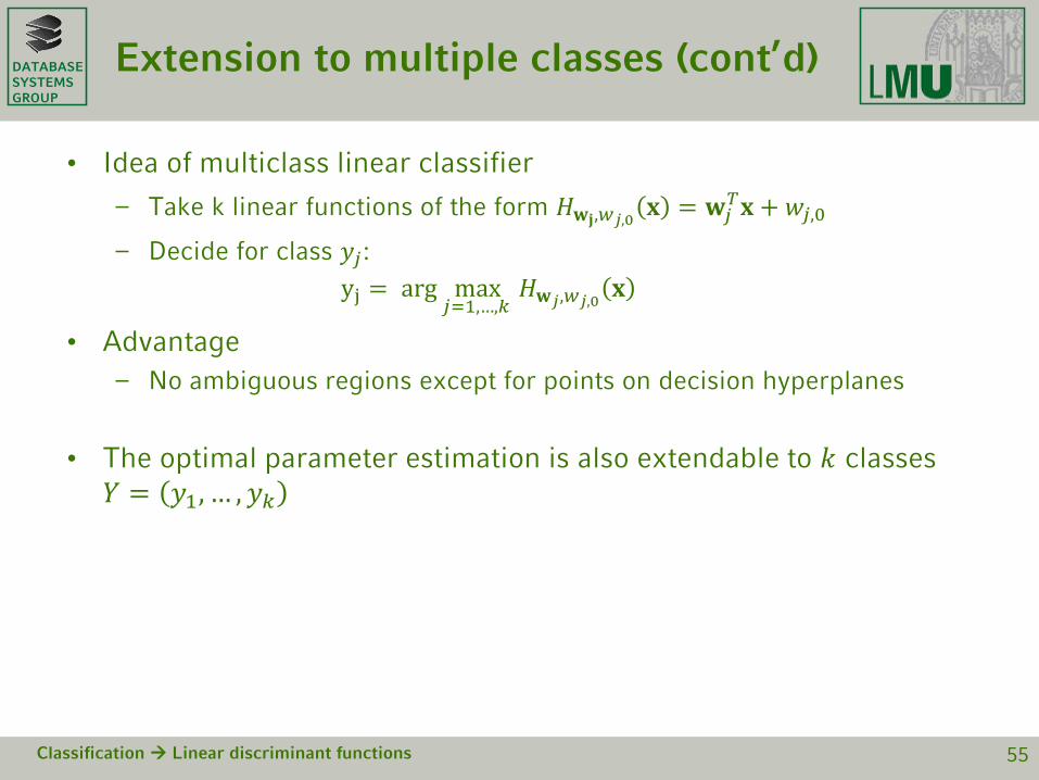
• Idea of multiclass linear classifier
– Take k linear functions of the form 𝐻𝐻𝐰𝐰𝐣𝐣,𝑙𝑙𝑗𝑗,0 𝐱𝐱 = 𝐰𝐰𝑗𝑗𝑇𝑇𝐱𝐱 + 𝑙𝑙𝑗𝑗,0
– Decide for class 𝑦𝑦𝑗𝑗: yj = arg max
𝑗𝑗=1,…,𝑘𝑘𝐻𝐻𝐰𝐰𝑗𝑗,𝑙𝑙𝑗𝑗,0 𝐱𝐱
• Advantage– No ambiguous regions except for points on decision hyperplanes
• The optimal parameter estimation is also extendable to 𝑘𝑘 classes 𝑌𝑌 = 𝑦𝑦1, … , 𝑦𝑦𝑘𝑘
Classification Linear discriminant functions 55

DATABASESYSTEMSGROUP
Discussion (SSE)
• Pro– Simple approach
– Closed form solution for parameters
– Easily extendable to non-linear spaces (later on)
• Contra– Sensitive to outliers not stable classifier
• How to define and efficiently determine the maximum stable hyperplane?
– Only good results for linearly separable data
– Expensive computation of selected hyperplanes
• Approach to solve the problems– Support Vector Machines (SVMs) [Vapnik 1979, 1995]
Classification Linear discriminant functions 56