263

CHAPTER- 6

ANALYSIS OF VERY FAST TRANSIENTS IN GIS USING

WAVELET TRANSFORMS

6.1 INTRODUCTION

Very Fast Transient Over voltages (VFTOs) and the associated Very

Fast Transient Currents (VFTCs) generated during switching operations in a

Gas Insulated Substation (GIS) couple conductively and inductively to the

secondary equipment connected to the GIS [89]. The frequency spectrum of

the VFTC gives the dominant frequencies present but cannot provide the

time varying current amplitude with respect to any particular frequency.

Since the transient response of the control circuits is a function of the

frequency content of the VFTC, it becomes necessary to segregate the VFTC

waveform both in time and frequency scale simultaneously. This has been

achieved by employing the GABOR wavelet function and the time-frequency

spectrum of the VFTC waveform has been calculated at various locations for

a 245kV GIS during a switching event.

6.2 INTRODUCTION TO WAVELETS

It is clear that any non-stationary signal can be analyzed with the

wavelet transforms. Time-frequency analysis of non-stationary signals

indicates the time instants at which different frequency components of the

signal come into reckoning. One direct consequence of such a treatment will

be the possibility to accurately locate in time all rapid changes in the signal

264

and estimate their frequency components as well.

Wavelet Theory is the mathematics associated with building a model

for a non-stationary signal, with a set of components that are small waves,

called wavelets. Informally, a wavelet is a short-term duration wave. These

functions have been proposed in connection with the analysis of signals,

primarily transients in a wide range of applications.

6.3 MATHEMATICAL BACKGROUND

To obtain a specific representation one has to decompose a signal X

into elementary building blocks Xi, of some importance as X = Σ Xi, where the

Xi’s are simple waveforms. In order to practically decompose a signal, we

need a fast algorithm in order to do it, since otherwise a practical

decomposition / representation might be only of theoretical importance. Once

we have the building blocks, we might attempt yet another task;

approximation, i.e. we try to get as good a performance of the original signal

as possible with only a few of the building blocks. We approach the original

signal by successively adding details to it, i.e. by successively refining it.

One of the classic tools to achieve such different representations of a signal is

the Fourier theory, for which we have a whole arsenal of tools at our disposal

from the purely continuous time, such as the Fourier integral, to discrete

time and the Fast Fourier Transform (FFT) algorithm. If we are given a pure

frequency signal eiωt, Fourier based methods will isolate a peak at the

frequency ω. However, already when confronted with the case of a signal built

of two pure oscillations occurring in two adjacent intervals, i.e. eiω1tX[a,b](t) +

265

eiω2tF[b,c](t), we run into problems: we obtain two peaks, without localization in

time. This immediately points out to the need for a time-frequency

representation of a signal, which would give us local information in time and

frequency.

6.4 CAPABILITIES OF WAVELET ANALYSIS

One major advantage afforded by wavelets is the ability to perform local

analysis that is, to analyze a localized area of a larger signal. When wavelets

are compared with sine wave, which is the basis of Fourier analysis,

sinusoids do not have limited duration, they extend from minus to plus

infinity. Where sinusoids are smooth and predictable, wavelets tend to be

irregular and asymmetric [107]. Fourier analysis consists of breaking up a

signal into some waves of various frequencies. Similarly, wavelet analysis is

the breaking up of a signal into shifted and scaled versions of the original (or

mother) wavelet. This has been explained clearly in the previous section.

6.5 BASIC CONCEPTS OF WAVELETS

Informally, a wavelet is a short-term duration wave. These functions

have been proposed in connection with the analysis of signals, primarily

transients in a wide range of applications. The basic concept of wavelet

analysis is the use of a wavelet as a kernal function [108] in integral

transforms and series expansion like sinusoid is used.

266

6.5.1 Continuous Wavelet Transform (CWT)

The continuous wavelet transform (CWT) was developed as an

alternative approach to short time Fourier transform (STFT).

The continuous wavelet transform is defined as follows:

*

,( , ) ( ) ( )

b aCWT b a f t t dtψ= ∫ (6.5.1)

Where * denotes complex conjugation. This equation shows how a function

f(t) is decomposed into a set of basis functions ψb,a(t), called the wavelet, and

the variables 'a' and 'b', scale and translation, are the new dimensions after

the wavelet transform.

The inverse wavelet transform of the above is given as

,

( ) ( , ) ( )b a

f t CWT b a t dbdaψ= ∫∫ (6.5.2)

The wavelets are generated from a single basic wavelet ψ (t), so-called

mother wavelet, by scaling and translation:

, ( ) 1 / ( / )b a t a t b aψ ψ= − (6.5.3)

In equation (6.5.3), 'a' is the scale factor, 'b' is the translation factor and the

factor 1/√a is for energy normalization across the different scales.

There are some conditions that must be met for a function to qualify as a

wavelet:

• Must be oscillatory

• Must decay quickly to zero (can only be non-zero for a short period of the

wavelet function).

• Must integrate to zero (i. e., the dc frequency component is zero)

267

These conditions allow the wavelet transform to translate a time-domain

function into a representation that is localized both in time (shift or

translation) and in frequency (scale or dilation). The time-frequency is used to

describe this type of multi resolution analysis. The selection of the mother

wavelet depends on the application. Scaling implies that the mother wavelet

is either dilated or compressed and translation implies shifting of the mother

wavelet in the time domain.

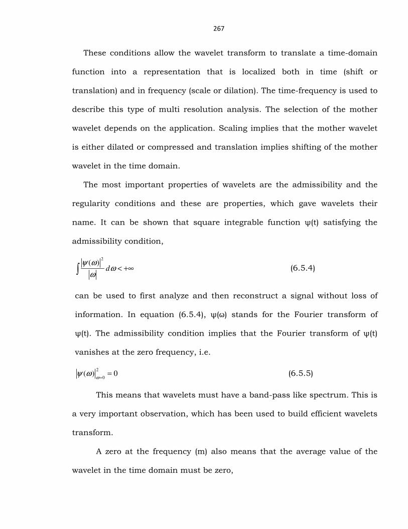
The most important properties of wavelets are the admissibility and the

regularity conditions and these are properties, which gave wavelets their

name. It can be shown that square integrable function ψ(t) satisfying the

admissibility condition,

2( )

dψ ω

ωω

< +∞∫ (6.5.4)

can be used to first analyze and then reconstruct a signal without loss of

information. In equation (6.5.4), ψ(ω) stands for the Fourier transform of

ψ(t). The admissibility condition implies that the Fourier transform of ψ(t)

vanishes at the zero frequency, i.e.

2

0( ) 0

ωψ ω

== (6.5.5)

This means that wavelets must have a band-pass like spectrum. This is

a very important observation, which has been used to build efficient wavelets

transform.

A zero at the frequency (m) also means that the average value of the

wavelet in the time domain must be zero,

268

( ) 0t dtψ =∫ (6.5.6)

As can be seen from Equation (6.5.6), the wavelet transform of a one-

dimensional function is two-dimensional; the wavelet of a two-dimensional

function is four dimensional, the time-bandwidth product of the wavelet

transform is the square of the input signal and for most practical applications

this is not a desirable property [109]. Therefore, one imposes some additional

conditions on the wavelet functions in order to make the wavelet transform

decrease quickly with decreasing scale 'a'. These are the reliability conditions

and they state that the wavelet function should have some smoothness and

concentration in both time and frequency domains. Regularity is complex

concept.

6.6 SCALING

The parameter scale (or dilation) in the wavelet analysis is similar to

the scale used in maps. As in the case of maps, high scales correspond to a

non-detailed global view (of the signal), and low scales correspond to a

detailed view. Similarly, in terms of frequency, low frequencies (high scales)

correspond to global information of a signal (that usually spans the entire

signal), whereas high frequencies (low scales) correspond to detailed

information of a hidden pattern in the signal (that usually lasts a relatively

short time). Fortunately in practical applications, low scales (high

frequencies) do not last for the entire duration of the signal. High scales (low

frequencies) usually last for the entire duration of the signal.

Scaling, as a mathematical operation, either dilates or compresses a

269

signal. Larger scales correspond to dilated (or stretched out) signals and

small scales correspond to compressed signals. All the signals given in the

Figures are derived from the same cosine signal, i.e., they are dilated or

compressed versions of the same function.

In terms of mathematical functions, if f(t) is a given function, it

corresponds to a contracted (compressed) version of f(t) if a > 1 and to an

expanded (dilated) version of f(t) if a < 1. However, in the definition of the

wavelet transform, the scaling term is used in the denominator, and

therefore, the opposite of the above statements holds, i.e., scales a > 1

dilates the signals where scales a <1, compresses the signal. This

interpretation of scale will be used throughout this text.

6.7 WAVELET FAMILIES

6.7.1 Mexican Hat Wavelet

Wavelets equal to the second derivative of a Gaussian function are

called Mexican Hats (MH). They were first used in computer vision to detect

multi scale edges. The MHW that has been used is as given by equation

(6.7.1)

22( ) (1 2 ) tt t eψ −= − (6.7.1)

This is obtained by taking the second derivative of the Gaussian function

6.7.2 Morlet Wavelet

The Morlet wavelet is arguably the 'original' wavelet. Although the

discrete Haar wavelets predate Morlet’s, it was only as a consequence of

Morlet’s work that the mathematical foundations of wavelets were found a

270

better formulation of time frequency methods [110].

Conceptually related to windowed-Fourier analysis, the Morlet wavelet is a

locally periodic wave train. It is obtained by taking complex sine wave and by

localizing it with a Gaussian (bell - shaped) envelops.

The Morlet wavelet is defined as:

2 2 2/ 2 / 4( ) [ ]e i tt Ce e e

α π π αψ = − (6.7.2)

This equation (6.7.2), it is a complex wavelet, which can be

decomposed into two parts, one for the real part and the other for the

imaginary part.

2 2 2/ 2 / 4( ) [cos( ) ]e

realt Ce t e

α π αψ π= − (6.7.3)

2 2 2/ 2 / 4( ) [sin( ) ]e

imagt Ce t e

α π αψ π−= − (6.7.4)

Where 'C' is the scaling parameter, which effects the width of window

and 'α' (alpha) is the modulation parameter. The Morlet wavelet is, by

definition, a complex function that contains phase information. For the

purpose of this project, only the real part of the Morlet wavelet is considered.

6.7.3: Discrete Wavelet Transform

Wavelet analysis employs a prototype function called the mother

wavelet. This function has a mean zero and sharply decays in an oscillatory

fashion, i.e., it sharply falls to zero on either side of its path. The wavelet

transform can be accomplished in two different ways depending on what

information is required out of this transformation process. The first method is

a continuous wavelet transform (CWT), where one obtains a surface of

271

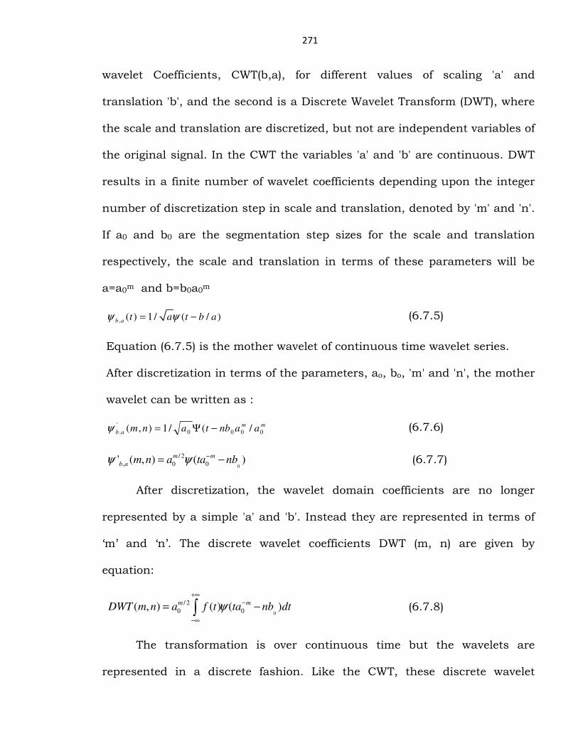
wavelet Coefficients, CWT(b,a), for different values of scaling 'a' and

translation 'b', and the second is a Discrete Wavelet Transform (DWT), where

the scale and translation are discretized, but not are independent variables of

the original signal. In the CWT the variables 'a' and 'b' are continuous. DWT

results in a finite number of wavelet coefficients depending upon the integer

number of discretization step in scale and translation, denoted by 'm' and 'n'.

If a0 and b0 are the segmentation step sizes for the scale and translation

respectively, the scale and translation in terms of these parameters will be

a=a0m and b=b0a0m

, ( ) 1 / ( / )b a t a t b aψ ψ= − (6.7.5)

Equation (6.7.5) is the mother wavelet of continuous time wavelet series.

After discretization in terms of the parameters, ao, bo, 'm' and 'n', the mother

wavelet can be written as :

mm

ab aanbtanm 0000

'

, /(/1),( −Ψ=ψ (6.7.6)

0

/ 2

, 0 0' ( , ) ( )m m

b am n a ta nbψ ψ −= − (6.7.7)

After discretization, the wavelet domain coefficients are no longer

represented by a simple 'a' and 'b'. Instead they are represented in terms of

‘m’ and ‘n’. The discrete wavelet coefficients DWT (m, n) are given by

equation:

0

/ 2

0 0( , ) ( ) ( )m mDWT m n a f t ta nb dtψ

+∞

−

−∞

= −∫ (6.7.8)

The transformation is over continuous time but the wavelets are

represented in a discrete fashion. Like the CWT, these discrete wavelet

272

coefficients represent the correlation between the original signal and wavelet

for different combinations of ‘m’ and ‘n’.

6.8 Wavelet Systems

There are several wavelet systems to implement wavelet transforms in

wavelet analysis, such has Haar, Daubechies, Symlets, Meyer and Shannon,

etc.

Haar and Daubechies Wavelets

Ingrid Daubechies, one of the brightest stars in the world of wavelet

research, invented what are called compactly supported wavelets – thus

making discrete wavelet analysis practicable. The name of the Daubechies

family wavelets is written as dbN, where N is the order, and 'db the

"surname" of the wavelet. The 'db' 1 is same as Haar wavelet. Haar is the

simplest wavelet basis. The scaling function φ(x) and primary wavelet ψ(x) are

given in equations below. These functions are defined recursively, as linear

combinations of scaled and shifted versions of φ(x), which is defined by the

fundamental recursion.

( ) (2 )kk z

x a x kφ φ∈

= −∑ (6.8.1)

such that

( ) 1x dxφ =∫ (6.8.2)

and ψ(x) is defined as

1( 1)( ) (2 )k kk zx a x kψ φ+∈ −

= +∑ (6.8.3)

The coefficients ak are the wavelets expansion coefficients. It is from the

273

restrictions on these values that the wavelet functions derive their properties,

such as orthogonal. The restrictions on the wavelet expansion coefficients are

the wavelet conditions as follows:

2kk z

a∈

=∑ (6.8.4)

The wavelet has compact support only if a finite number of the wavelet

coefficients 'a', and 'b' are non-zero. Haar wavelet is a scaling function, given

in equation (6.8.1). The function φ(x) will be zero in the real time except for

the region 0+ to 1; and 1 at x=1.

6.9 WAVELET ANALYSIS OF TRANSIENT SIGNALS

Wavelets are developing very rapidly in the recent years, and there are

many wavelet functions that have evolved, for example Morlet, Mexican Hat,

Haar, Daubechies , etc. But it is very important to choose the suitable

wavelet for the analysis of the selected problem. In the last few years many

authors suggested Mexican Hat for analysis of transient signals [105], and

some authors suggested Morlet [107, 108]. The Gabor, Daubechies, Haar

and Morlet wavelets, which are employed for analysis of transient signals. In

this thesis the Gabor wavelet is used to analyze VFTC. It is proposed that

proper selection of mother wavelet on the basis of nature of transients, to

improve the quality Time - frequency spectrums. In this case, the selection of

mother wavelet is on the basis of nature of transients (very high frequency);

particularly Gabor wavelet is very much suitable for time-frequency analysis.

The direct advantage of this is more accurate location of time for all abrupt

changes in the signal and estimates their frequency components. The

274

transient voltages and currents are obtained from EMTP-RV simulation

network as shown in the Fig.6.2. In this analysis the wavelet transforms are

performed on the required transient signals. Different soft wares were

developed and utilized for analysis. FFT software is employed for calculation

of dominant frequencies in the signals for the calculation of the dilation

factor used in wavelet transform. To perform continuous wavelet analysis for

VFTO/VFTC signals, two special programs were developed using MATLAB.

The programs are developed using Gabor wavelet function, for the wavelet

analysis. The “WAVELET TOOLBOX” in MATLAB software of Version 7.1,

(product of The Math Works) is used for Discrete and Continuous Wavelet

Analysis. The WAVELET TOOLBOX is a collection of functions built on the

MATLAB technical computing environment. It provides tools for the analysis

and synthesis of signals, tools for statistical applications, using wavelets and

wavelet packets within the framework of MATLAB. It provides an excellent

interface to explore the various aspects and applications of wavelets.

After the wavelet analysis on the required signals, the resulting graphs

are obtained using Picture files and .emf files available in Wavelet Toolbox

which is powerful and one of the best data visualization software. For

plotting and data visualization MATLAB programs and tools are extensively

used because of its unique combination of power, speed and ease of use and

other features. Its user interface is very useful and provides capability to

interactively explore and understand the data change plotting options, etc.

In this theoretical work, Mexican Hat (MH) and Morlet Wavelets (MW)

275

are used to determine time-frequency response of different shapes of

transient voltages/currents. The primary aim of the analysis is to determine

the changes in frequency with the decrease in values of dilation coefficient 'a'

and to obtain the limiting values for detection of perturbation.

6.10 TIME-FREQUENCY ANALYSIS OF VFTOs/VFTCs IN GIS SYSTEMS

Several authors have used transfer function approach to determine the

frequency response characteristics of such voltage pulses. However, this

method can be used for determining frequency characteristics only. Non-

stationary signals can be analyzed with wavelet technique. There are number

of ways in which the input signal can be subjected to time-frequency

analysis and among them, the wavelet transform is popular. The direct

consequence of this approach is the possibility to accurately locate in time,

all abrupt changes in the signal and estimate their frequency components as

well. Wavelets were developed independently in the field of mathematics,

quantum physics, seismic geology, and electrical engineering. Interchange

between these fields led to many new wavelet applications such as signal

compression, noise elimination, image compression, turbulence, human

vision radar, earthquake prediction, etc. Similarly, in electrical power

systems, the wavelet approach can be applied for analysis very high

frequency transients. The advantage of the most useful features of wavelets

is the effectiveness of defining coefficient for a given wavelet system to be

adopted for a given problem. In GIS systems, Very Fast Transient Over

voltages (VFTOs) are mainly due to switching operations. These transient

276

over voltages and the associated Very Fast Transient Currents (VFTC)

have rise times in the order of 4 to 50ns[20]. The peak magnitude of the

transient current may be about a few kA depending on the location of the

switch operated, the substation layout and the distance of the observation

point from the switch. These transients are a possible source of

electromagnetic interference (EMI) to the electronic equipments

operating within the GIS. Both the conducted and the radiated

mechanisms are responsible for the coupling of the VFTC to the control

circuitry present within the GIS. Each switching operation produces several

VFTC and hence numerous transient EM fields are generated. The number

of transients can vary with the rated voltage of the substation, type and

location of the switch operated, and speed of the switch and the electrical

characteristics of the high voltage bus being operated [112]. Many authors

have reported malfunctioning of the primary/secondary equipments

during switching operations in a GIS [113]. The transient voltages getting

coupled to control and protection circuits are highly sensitive to the

frequency content of VFTC. In view of the above, a technique is proposed in

this chapter for segregating the VFTC waveforms in both time and frequency

scale simultaneously. The variation of the amplitude of VFTC with distance

and time, dominant frequency components of the VFTC and variation in

the frequency content of VFTC with distance have been analyzed. Even

though, the characterization based on the above approach gives variation of

the amplitude and frequency content of the VFTC with distance, it cannot

277

provide the time varying current waveforms for dominant frequencies

associated with the VFTC. Such variation of the current magnitude with

frequency at various locations of the GIS is required, to know the critical

frequencies that are responsible for the transients induced in the control

circuitry. In the present study, a wavelet model is proposed to

evaluate the time- frequency spectra of VFTC waveforms. The model

has been validated, by evaluating the time varying transient

waveforms at different frequencies associated with an arbitrary

transient signal. Using these results as a source, the time-frequency spectra

of the VFTC waveforms are obtained at various locations of a 245kV GIS

during a Disconnector switch opening event is evaluated. By

reconstructing the VFTC waveform using the transient current waveforms

obtained at different frequencies, the wavelet model has been validated for

the present application. The proposed wavelet technique based model is

found to be effective for the characterization of VFTC waveform in time

and frequency scale simultaneously. During various switching the

VFTO is considered as a non-stationary high frequency signal whose

properties change or evolve in time. Wavelets are mathematical functions

that divide the data into different frequency components, and then study

each component with a resolution matched to its scale.

6.11. VERY FAST TRANSIENT CURRENTS (VFTC)

In this chapter, the time-frequency analysis of very fast transient

current (VFTC) waveform at two different locations has been carried out. The

278

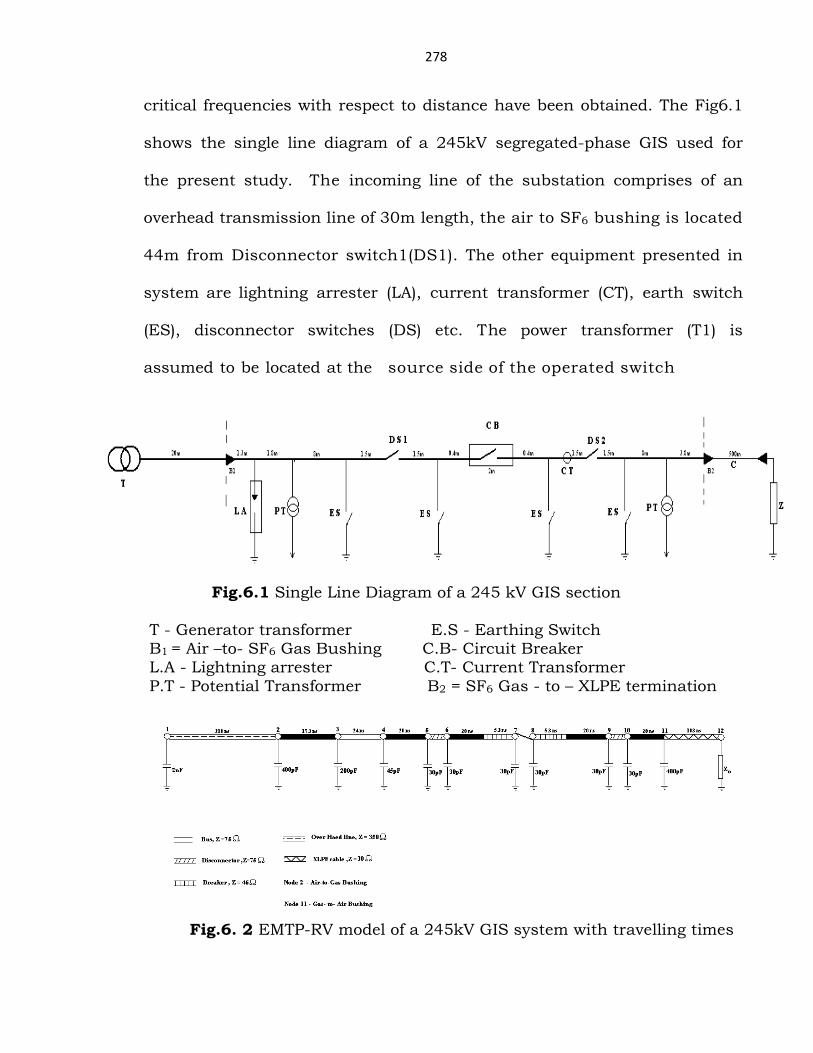
critical frequencies with respect to distance have been obtained. The Fig6.1

shows the single line diagram of a 245kV segregated-phase GIS used for

the present study. The incoming line of the substation comprises of an

overhead transmission line of 30m length, the air to SF6 bushing is located

44m from Disconnector switch1(DS1). The other equipment presented in

system are lightning arrester (LA), current transformer (CT), earth switch

(ES), disconnector switches (DS) etc. The power transformer (T1) is

assumed to be located at the source side of the operated switch

Fig.6.1 Single Line Diagram of a 245 kV GIS section

T - Generator transformer E.S - Earthing Switch B1 = Air –to- SF6 Gas Bushing C.B- Circuit Breaker L.A - Lightning arrester C.T- Current Transformer P.T - Potential Transformer B2 = SF6 Gas - to – XLPE termination

Fig.6. 2 EMTP-RV model of a 245kV GIS system with travelling times

279

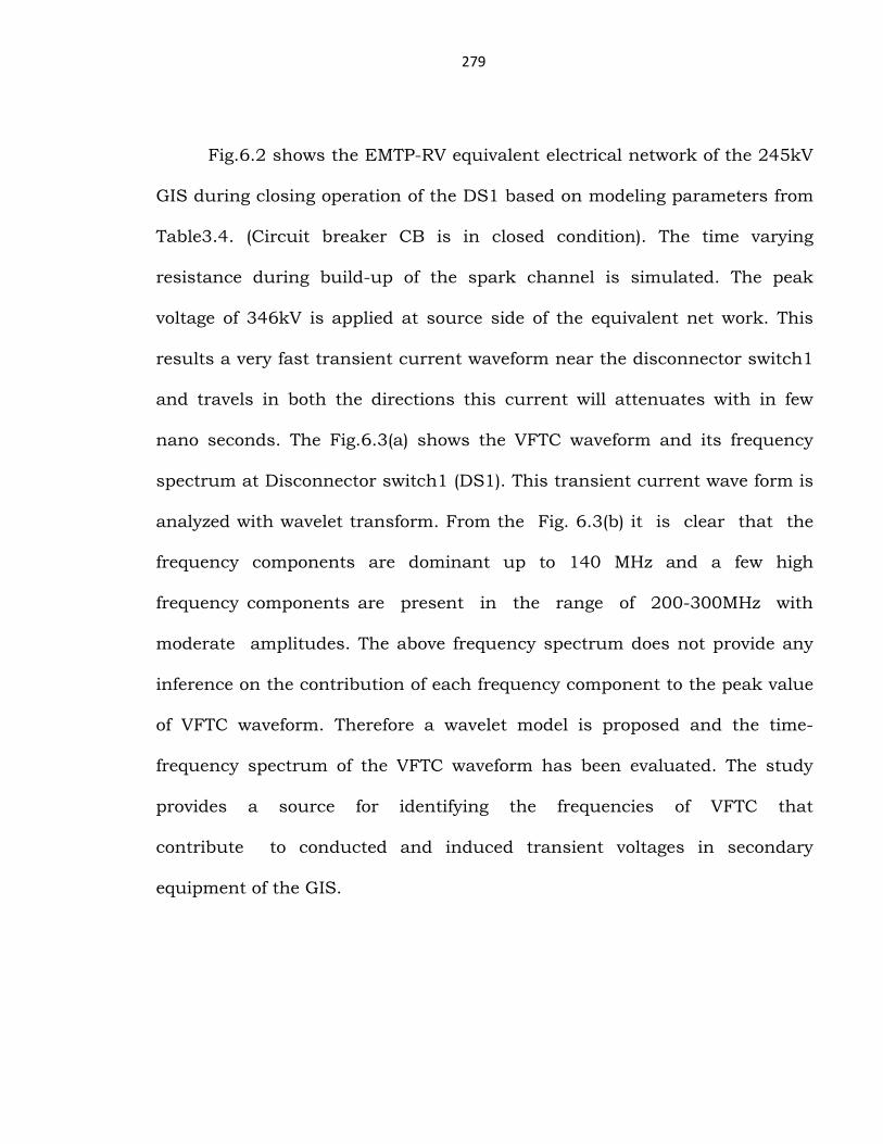
Fig.6.2 shows the EMTP-RV equivalent electrical network of the 245kV

GIS during closing operation of the DS1 based on modeling parameters from

Table3.4. (Circuit breaker CB is in closed condition). The time varying

resistance during build-up of the spark channel is simulated. The peak

voltage of 346kV is applied at source side of the equivalent net work. This

results a very fast transient current waveform near the disconnector switch1

and travels in both the directions this current will attenuates with in few

nano seconds. The Fig.6.3(a) shows the VFTC waveform and its frequency

spectrum at Disconnector switch1 (DS1). This transient current wave form is

analyzed with wavelet transform. From the Fig. 6.3(b) it is clear that the

frequency components are dominant up to 140 MHz and a few high

frequency components are present in the range of 200-300MHz with

moderate amplitudes. The above frequency spectrum does not provide any

inference on the contribution of each frequency component to the peak value

of VFTC waveform. Therefore a wavelet model is proposed and the time-

frequency spectrum of the VFTC waveform has been evaluated. The study

provides a source for identifying the frequencies of VFTC that

contribute to conducted and induced transient voltages in secondary

equipment of the GIS.

280

Fig.6.3 (a) VFTC Waveform at DS1 from EMTP-RV simulation

Fig. 6.3(b) Frequency Spectrum of VFTC at DS1

281

6.12 Proposed Wavelet Model

The wavelet transform W (b,a) of a function I(t) with respect to a given

mother wavelet , is defined as[104]:

/�K, Y� = 1√K Z Ψ [� − Y

K \ @����� �6.12.1�∞

<∞

K = 12Π& �6.12.2�

Where, a= Scale parameter,

b=Translation parameter

f = frequency

Gabor wavelet function is given by

��� = ]<[�"^"\_�`� �6.12.3�

Where a� is a constant control the

band of the frequencies to be identified

/�K, Y� = 1√K Z &���]<b�<c

L d^"

∞

<∞

_�` [� − YK \ �� �6.12.4�

Where, σ 2 is a constant and controls the band of the frequencies to be

identified. The VFTC waveform has been considered for the time duration of

2µs and time-localization window is moved from 0 to µs by the translation

parameter.

282

Validity of the proposed wavelet method

The aim of the present analysis is to segregate the VFTC waveform into

the time varying current waveform with dominant frequency. In order to

estimate the time varying current waveform at a particular frequency, it is

essential to determine the multiplication factor (k). This factor converts the

wavelet transform of the VFTC waveform at a particular scale

parameter ‘a’ into the transient current waveform for the corresponding

frequency (f =1/2a). The selection of σ 2 value is based on the

accuracy with which the output waveform (wavelet transform of the

input waveform) at a particular scale parameter matches with the input

/original waveform. To confirm the validity of σ2 value and the multiplication

factors at different frequencies, a sinusoidal signal with amplitude of 1p.u.

for various frequencies ranging from 5 to 200MHz is considered. Table 6.1

shows the variation of k values with σ 2 at a particular frequency.

Similarly, k values have been listed in Table 6.2 for different frequencies at a

particular value of σ 2. From these results, it is evident that the k value

decreases with increase of σ 2

and the value of k2/f is constant for a

particular value of σ 2 Fig.6.4(a-b) shows the Gabor mother wavelet for the

frequency of 200 MHz at σ 2= 4 and 64.

283

Table 6.1 Variation of k w.r.t. σ 2

Frequency(MHz)

σ 2

K

5.0

2.0 3989.0

3.0 3478.3

4.0 3105.4

16.0 1581.1

64.0 791.4

128.0 559.0

Table 6.2 Variation of k w. r. t. Frequency.

σ 2

Frequency

(MHz)

k

K2/f

64.0

5.0 791.4 0.1253

30.0 1936.5 0.1250

50.0 2500.0 0.1250

100.0 3541.7 0.1254

200.0 5010.0 0.1255

284

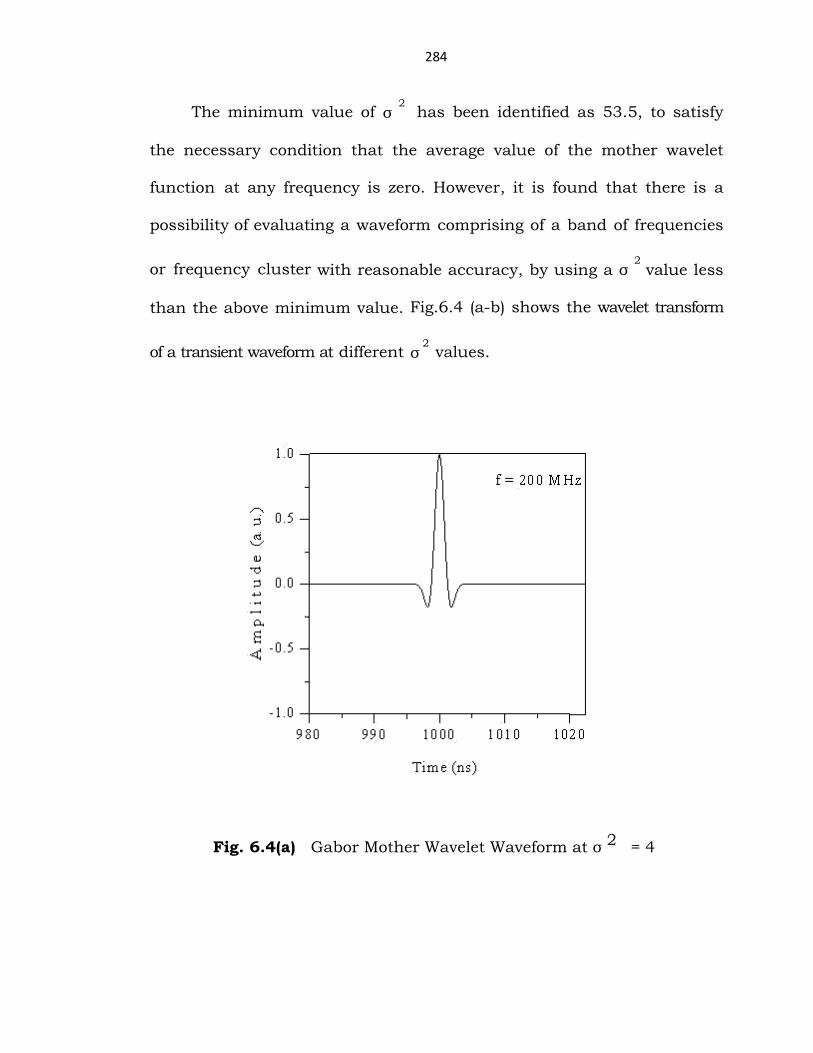
The minimum value of σ 2 has been identified as 53.5, to satisfy

the necessary condition that the average value of the mother wavelet

function at any frequency is zero. However, it is found that there is a

possibility of evaluating a waveform comprising of a band of frequencies

or frequency cluster with reasonable accuracy, by using a σ 2 value less

than the above minimum value. Fig.6.4 (a-b) shows the wavelet transform

of a transient waveform at different σ 2 values.

Fig. 6.4(a) Gabor Mother Wavelet Waveform at σ 2 = 4

285

Fig. 6.4(b) Gabor Mother Wavelet Waveform at σ 2 =64

At σ 2 = 4, however there is a small difference in the first quarter

cycle of the output waveform (wavelet transform of input waveform)

compared to the input waveform, the peak magnitude is observed

to be the same. For σ 2 = 64, the output waveform takes a minimum of

one time cycle to reach closer to original waveform with reasonable

accuracy. Similarly, for σ 2

=256, the output waveform takes one more

time cycle to match the original waveform. These results suggest that

the number of time cycles required for the output waveform to match

the original waveform increase with the increase of σ 2 value. Thus,

for reproducing as it is at a particular frequency, it is necessary to

286

keep σ 2 value less than or equal to 4.The validity of the model is

confirmed by comparing the original arbitrary transient signal with the

reconstructed transient signal, obtained by summing up the transient

waveforms at different frequencies. The validity of the model is further

established, by comparing the amplitudes of the dominant frequencies

from the frequency spectra of the above two signals i.e., the

reconstructed and the original. Using these results as a basis, VFTC

waveforms obtained at various locations of a 245kV GIS during the

proposed switching operation are segregated.

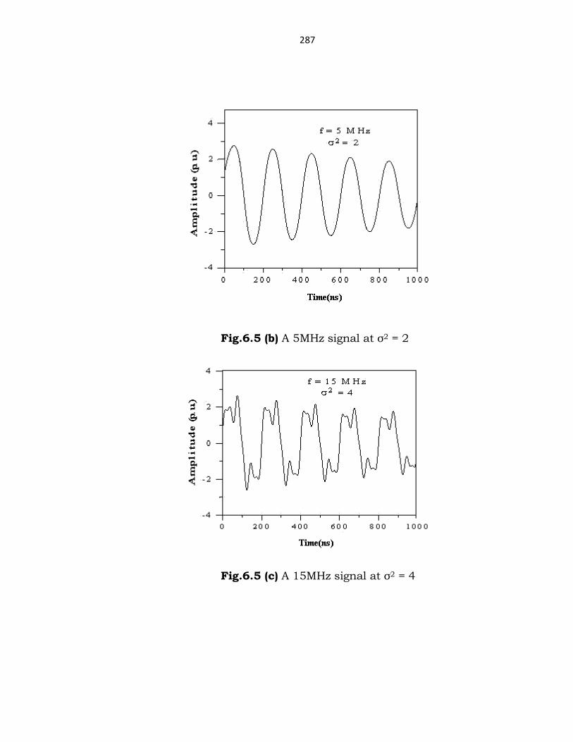
Fig.6.5 (a) Original wave form of the arbitrary signal

287

Fig.6.5 (b) A 5MHz signal at σ2 = 2

Fig.6.5 (c) A 15MHz signal at σ2 = 4

288

Fig.6.5 (d) A 15MHz signal at σ2 =64

Fig.6.5 (e) A 30MHz signal at σ2 =64

289

Fig.6.5 (f) A 50MHz signal at σ2 =128

Fig.6.5 (g) A 100MHz signal at σ2 =64

290

Fig.6.5 (h) A reconstructed waveform of arbitrary signal

Fig.6.5 (a-h) Validation of the Wavelet model for an arbitrary

transient signal.

6.13 RESULTS

The VFTC waveforms necessary for the study have been

calculated at important locations of a 245kV GIS during a switching

condition, using EMTP-RV. Fig 6.6(a) and 6.6(b) shows the VFTC

waveform at Air–SF6 bushing in time and frequency scale respectively.

The Fig6.8 shows the time-frequency spectrum of the VFTC waveform at

the DS1.

291

Fig. 6.6(a) VFTC Waveform at Air - SF6 bushing

Fig. 6.6(b) Frequency Spectrum of VFTC Waveform at Air -

SF6 bushing

292

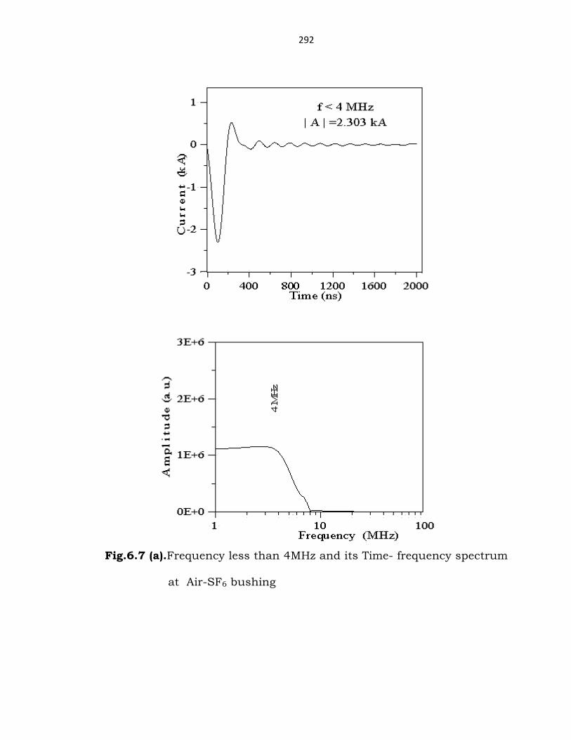
Fig.6.7 (a).Frequency less than 4MHz and its Time- frequency spectrum

at Air-SF6 bushing

293

Fig. 6.7(b) Frequency equal to 7.5MHz and its Time-frequency

spectrum at Air - SF6 bushing

294

Fig.6.7 (c) Frequency equal to 13MHz and its Time-frequency spectrum

at Air - SF6 bushing

295

Fig.6.7(d) Frequency equal to 29.5MHz and its Time-Frequency

spectrum at Air - SF6 bushing

296

Fig.6.7(e). Frequency equal to or less than 51 MHz and its Time-

Frequency spectrum at Air - SF6 bushing

297

Fig. 6.7 (f). Time-Frequency Spectrum of the VFTC at Air - SF6

Bushing

298

It is observed from the Fig.6.7(a) to Fig.6.7(e), the peak magnitude

of the current waveforms for the frequency content < 4 MHz, 7.5

MHz, 13MHz, 29.5MHz and 51 MHz are 2.303 kA, 1.083kA, 0.961kA,

0.058kA and 0.054kA respectively. Accurate evaluation of the first

peak of the transient current waveform for the frequency content

less than 4MHz is of utmost significance to reconstruct the VFTC

waveform. This may be due to the higher attenuation rate of the

transient current amplitude with time for this frequency component.

Thus, for estimation of the above waveform, a frequency of 2.5 MHz and

σ 2= 3 has been used. The current waveforms at other dominant

frequencies have been calculated with σ 2= 32. The VFTC waveform at

Air - SF6 bushing is mostly contributed by the frequency components

less than or equal to 13MHz. The current waveform calculated for a

frequency of 51MHz is also associated with the signal of 44.5MHz

frequency as can be seen from Fig. 6.7(e). From the results, it is

confirmed that the frequency spectrum of the VFTC waveform (refer

Fig.6.6(b) and the frequency spectra of the current waveforms

evaluated at dominant frequencies using the wavelet model (refer

Fig.6.7(a-e) are closely identical. The validity of the calculation is

further verified by comparing the resultant waveform obtained by

summing up the transient current waveforms at different

frequencies i.e., the reconstructed VFTC waveform in Fig. 6.7(f)) with

299

the original VFTC waveform shown in Fig.6.6(a). Both the waveforms are

more or less identical except that there is a slight reduction in the

peak amplitude about 6.8% of the reconstructed VFTC waveform.

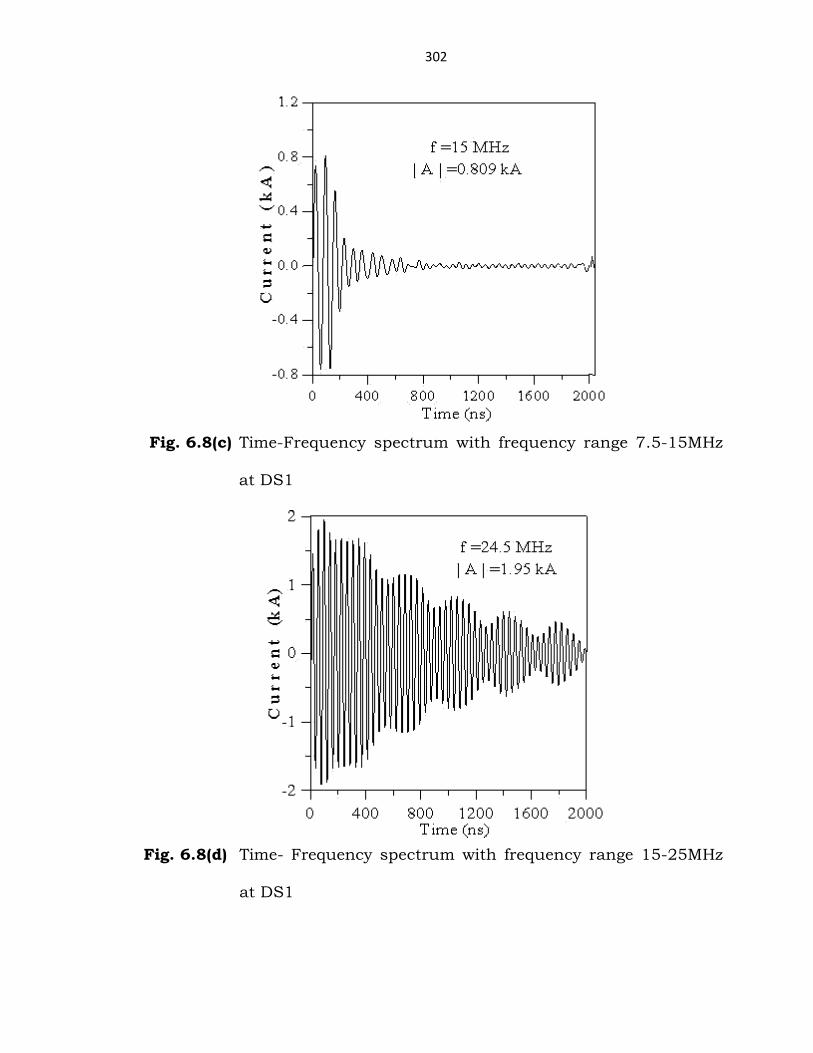
The Fig. 6.3(a) shows the transient current waveform at DS1 during the

switching operation of DS1 itself. From the Fig. 6.8(a) to 6.8(d) the peak

magnitudes of the current waveforms are observed for frequencies of < 4

MHz, 7.5 MHz, 15 MHz and 24.5 MHz are 2.46 kA, 2.18 kA, 0.809 kA

and 1.95 kA respectively. The current waveforms at all the frequencies

are found to be oscillatory and attenuating with time. The current

waveform for a frequency content less than 4 MHz is evaluated using a

scale parameter corresponding to the frequency of 3MHz and σ 2 =

4. The current waveforms at other dominant frequencies have been

evaluated using σ 2= 32 or 64 or 128 or 256. The transient current

waveform calculated for the frequency of 42.5MHz is also associated with

the signal of 44.5MHz frequency. Similarly, current waveform that was

calculated for frequency of 108.5MHz is associated with the waveforms

of 100 and 105 MHz The peak amplitude of transient current at 309 MHz

frequency is found to be about 0.5kA. It is clear that, higher value of σ 2

is required to evaluate current waveforms for the frequencies present

in the VFTC waveform at moderate/low levels. At this location also,

current magnitudes obtained at different frequencies may not be

directly proportional to the amplitudes obtained from the frequency

300

spectrum of the VFTC waveform. These results propose that the

attenuation rate of the transient current magnitude with time is

different for different frequencies associated with the VFTC. Finally,

from the Fig. 6.8(k) and 6.8(l) the model is validated by summing up the

current waveforms at different frequencies i.e., the reconstructed VFTC

waveform and compared with the original VFTC waveform. Both the

waveforms are identical except that there is a small reduction in the

peak magnitude (i.e., about 7.9 %) of the re-constructed waveform. This

may be due to those frequencies, which are inherent in the VFTC

waveform, but are neglected for the wavelet analysis and for the final

summation. To understand the effect of location of the observation

point on the peak amplitude of the transient current at different

frequencies in a 245kV GIS, wavelet analysis has been carried out

for VFTC waveforms at the DS1 and the Air-SF6 bushing locations.

The results are given in Table6.3. At the Air-SF6 bushing, which is at

a distance of 12.6m from DS1, the dominant frequencies are

possible up to 322MHz. The peak amplitude of the transient currents for

frequencies above 91.5MHz decreases from DS1 to the Air-SF6 bushing.

From the current amplitudes obtained at DS1 and the Air-SF6 bushing,

it is clear that high frequency components generated locally attenuate

within a few meters distance from their point of generation.

301

Fig. 6.8(a) Time- Frequency spectrum with frequency range 0-4MHz at

DS1

Fig. 6.8(b) Time-Frequency spectrum with frequency range 0-7.5MHz

at DS1

302

Fig. 6.8(c) Time-Frequency spectrum with frequency range 7.5-15MHz

at DS1

Fig. 6.8(d) Time- Frequency spectrum with frequency range 15-25MHz

at DS1

303

Fig. 6.8(e) Time-Frequency spectrum with frequency range 24-43MHz

at DS1

Fig. 6.8(f) Time-Frequency spectrum with frequency range 40-63MHz

at DS1

304

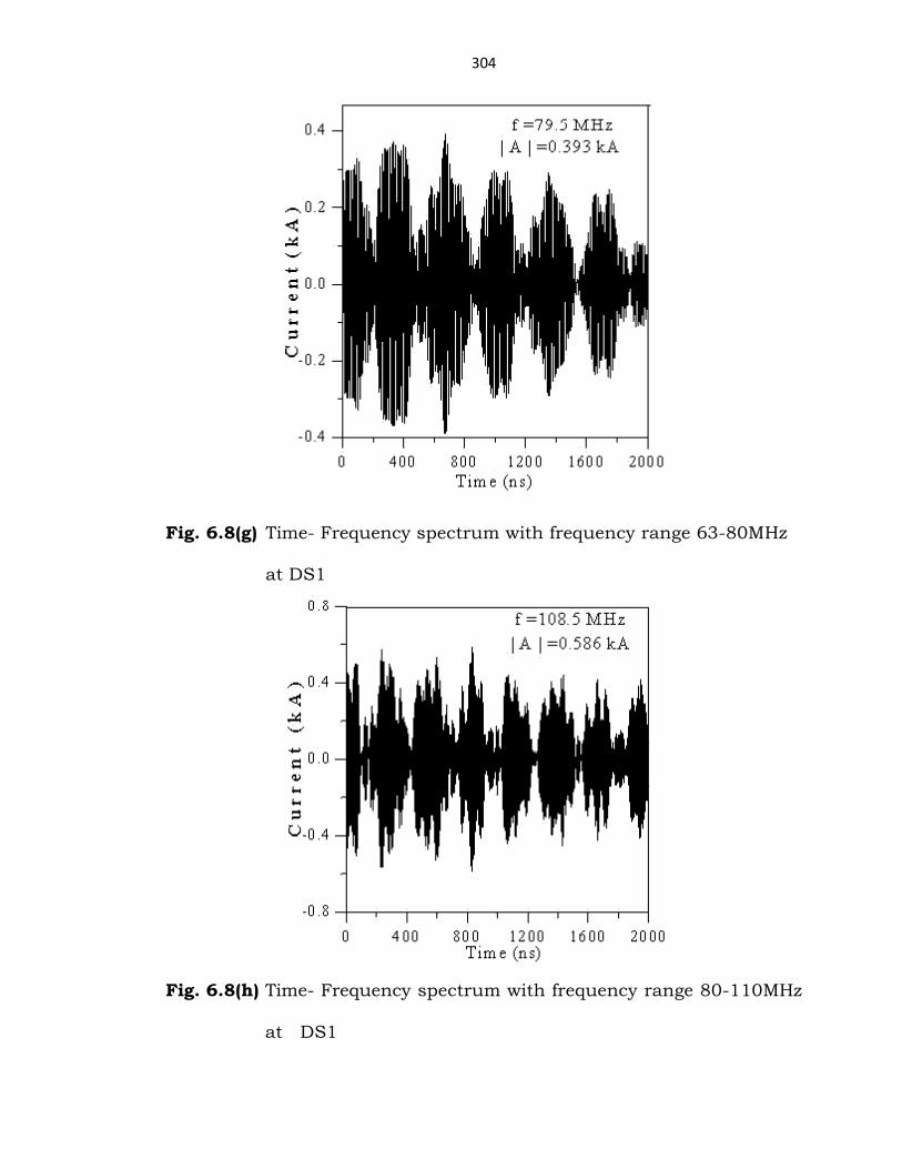
Fig. 6.8(g) Time- Frequency spectrum with frequency range 63-80MHz

at DS1

Fig. 6.8(h) Time- Frequency spectrum with frequency range 80-110MHz

at DS1

305

Fig. 6.8(i). Time-Frequency spectrum with frequency range 200-

310MHz at DS1

306

Fig. 6.8(j) VFTC waveform and its frequency spectrum using wavelet

transform at DS1

307

Table.6.3 Transient current amplitudes in kA during DS1 switching.

Frequency

(MHz)

At DS1

Air-SF6Bushing

4 2.460 2.303

7.5 2.180 1.083

13.0/15.0 0.809 0.961

21.5 - -

24.5 1.950 -

29.5 – 31.5 - 0.058

42.5-44.5 0.223 -

44.5-51.0 - 0.054

44.5 – 55.5 - -

62.0 0.209 -

72.0 - 87.5 - -

72.0 – 91.5 - -

79.5-82.5 0.393 -

100 – 108.5 0.586 -

121.5–135.0 - -

133.5–135.0 -

145.5 0.091 -

165.0 - -

200.0-205.0 0.200 -

230.0– 239.0 -

300.0-309.0 0.518 -

309.0-322.0 -

308

The transient current magnitude for the frequency content 100–

108.5 MHz is only 166 A at the DS1 location and is low compared to

585A at DS1. At the DS1 location, which is at a distance of 8.3 m from

the switch DS1, the dominant frequencies are limited to 135 MHz except

that there is a high frequency content in the range of 230-239MHz. The

transient current magnitude at DS1 location for the frequency of 230-

239 MHz is only 124 A, in contrast to the peak amplitude of 337A at the

Air-SF6 bushing. Further, the current magnitude for 24.5MHz frequency

at GIS-cable termination is only 58A, in contrast to 1.95kA at DS1.

From the analysis, it is observed that higher value of σ 2 > 64 is

acceptable, to evaluate the current waveforms for the dominant

frequencies, beyond 15MHz. The above frequency limit has been

identified based on attenuation rate of transient current magnitude

with time.Fig.6.10(a-c) shows the variation in peak amplitude of the

transient currents with frequency at various locations of a 245kV GIS

during the switching event under study. From this figure, it is seen that,

in general, at all positions of the GIS peak. The Current amplitude

decreases with increase of frequency. The contribution of very high

frequency components to the VFTC waveform at/near DS1 is

more compared to the other locations in the GIS. In order to understand

the variation in transient current level at different frequencies with

distance from the operated switch, current magnitude vs. distance

chart has been evaluated for various frequencies associated with

309

the VFTC waveforms.

Fig.6.9. Variation of peak amplitude of the transient current with

Frequency.

From the Fig.6.9, it is clear that the variation in amplitude of the

transient current for the low frequency content, i.e., less than 1.5 MHz

is almost flat. Beyond the frequency of 10.5 MHz, an oscillatory

variation in the peak magnitude of the transient current has been

observed as we move away from the location of the switch. This

oscillatory behavior may be due to the considerable surge capacitance

of the GIS components. More clearly, the GIS surge capacitance

converts high frequency transient current signal into the low

frequency signal. Further, the attenuation of the transient current

magnitude with distance has been observed to be significant for the

frequencies beyond 20.5MHz. For the entire frequency range of the

VFTC, the transient current magnitude is highest at/near the switch

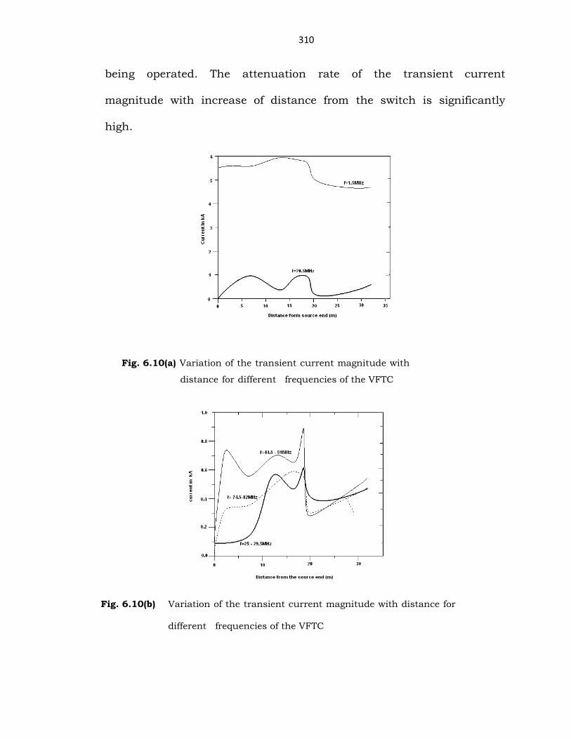
310

being operated. The attenuation rate of the transient current

magnitude with increase of distance from the switch is significantly

high.

Fig. 6.10(a) Variation of the transient current magnitude with

distance for different frequencies of the VFTC

Fig. 6.10(b) Variation of the transient current magnitude with distance for

different frequencies of the VFTC

311

Fig. 6.10(c) Variation of the transient current magnitude with distance for

different frequencies of the VFTC

“The data related to variation in the transient current

magnitudes with distance / frequency can be used as an excitation

for calculating the transient electromagnetic fields leaking out of the

GIS. More clearly, the transient current vs frequency chart at various

locations in a GIS will be helpful to identify critical frequencies of the

transient EM field emission from different modules of the GIS during

switching operations.”

6.13 SUMMARY

Time-Frequency spectrum of the VFTC waveform during

Disconnector switch operation has been evaluated at various locations of

a 245kV GIS by using proposed Gabor wavelet function. The variations

of current magnitude with time for different frequencies associated with

the VFTC are calculated. The variations in the transient current

magnitudes with distance / frequency have been estimated.

312

The current magnitudes at the DS1 location for all the frequencies

above 74.5MHz are found to be higher than the current levels that are

obtained at or near Air-to-SF6 Bushing. It is observed that the

current magnitude at the Air-to-SF6 Bushing is not considerable

beyond 13MHz and for frequency content less than 4 MHz, the

current magnitude is almost the same as that at the Disconnector

Switch1 operated.

The transient current magnitudes for frequency components of

200MHz and above at or near the Disconnector Switch1 operated

are in the order of a few hundred amperes. Further, the highest

transient current magnitudes at different frequencies are not directly

proportional to the amplitudes that are obtained from the

frequency spectrum of the VFTC waveform. It is also observed from

the results the attenuation of the current magnitude with time is

different for different frequencies of the VFTC. The wavelet analysis

also shows that the attenuation rate of the transient current magnitude

with distance has been observed to be significant for the frequencies

beyond 20.5MHz. It is concluded that the in GIS systems, the transient

current level decreases with increase of frequency component associated

with the VFTC waveforms. The proposed wavelet technique is very useful

in estimation of Time-frequency spectrum of VFTOs/VFTCs; hence

accurate shielding design is possible for GIS systems.