Embed Size (px)
Citation preview

Chapter 5. Separation of Variables
At this point we are ready to now resume our work on solving the three
main equations: the heat equation, Laplace’s equation and the wave equa-
tion using the method of separation of variables.
4.1 The heat equation
Consider, for example, the heat equation
ut = uxx, 0 < x < 1, t > 0 (4.1)
subject to the initial and boundary conditions
u(x, 0) = x− x2, u(0, t) = u(1, t) = 0. (4.2)
Assuming separable solutions
u(x, t) = X(x)T(t), (4.3)
shows that the heat equation (4.1) becomes
XT′ = X′′T,
which, after dividing by XT and expanding gives
T′
T=
X′′
X, (4.4)
implying that
T′ = λT, X′′ = λX, (4.5)
where λ is a constant. From (4.2) and (4.3), the boundary conditions be-
comes
X(0) = X(1) = 0. (4.6)

2 Chapter 5. Separation of Variables
Integrating the X equation in (4.5) gives rise to three cases depending on
the sign of λ but as seen in the last chapter, only the case where λ = −k2
for some constant k is applicable which we have as the solution
X(x) = c1 sin kx + c2 cos kx. (4.7)
Imposing the boundary conditions (4.6) shows that
c1 sin 0 + c2 cos 0 = 0, c1 sin k + c2 cos k = 0, (4.8)
which leads to
c2 = 0, c1 sin k = 0 ⇒ k = 0, π, 2π, . . . nπ, (4.9)
where n is an integer. From (4.5), we further deduce that
T(t) = c3e−n2π2t,
giving the solution
u(x, t) =∞
∑n=1
bne−n2π2t sin nπx,
where we have set c1c3 = bn. Using the initial condition gives
u(x, 0) = x− x2 =∞
∑n=1
bn sin nπx.
At this point, we recognize that we have a Fourier sine series and that the
coefficients bn are chosen such that
bn = 2∫ 1
0(x− x2) sin nπx dx
= 2[
1− 2xn2π2 cos nπx +
(x2 − x
nπ− 2
n3π3
)cos nπx
]∣∣∣∣1
0
=4
n3π3 (1− (−1)n).
Thus, the solution of the PDE as
u(x, t) =4
π3
∞
∑n=1
1− (−1)n
n3 e−n2π2t sin nπx. (4.10)

4.1. The heat equation 3
Figure 1 shows the solution at times t = 0, 0.1 and 0.2.
Example 1
Solve
ut = uxx, 0 < x < 1, t > 0 (4.11)
subject to
u(x, 0) = x− x2, ux(0, t) = ux(1, t) = 0. (4.12)
This problem is similar to the proceeding problem except the boundary
conditions are different. The last problem had the boundaries fixed at zero
whereas in this problem, the boundaries are insulated (i.e. no flux bound-
ary conditions). Assuming that the solutions are separable
u(x, t) = X(x)T(t), (4.13)
then from the heat equation, we obtain
T′ = λT, X′′ = λX, (4.14)
where λ is a constant. The boundary conditions in (4.12) become, accord-
ingly
X′(0) = X′(1) = 0. (4.15)
Integrating the X equation in (4.14) gives rise to again three cases depend-
ing on the sign of λ but as seen earlier, only the case where λ = −k2 for
some constant k is relevant. Thus, we have
X(x) = c1 sin kx + c2 cos kx. (4.16)
Imposing the boundary conditions (4.15) shows that
c1k cos 0− c2k sin 0 = 0, c1k cos k− c2k sin k = 0, (4.17)
which leads to
c1 = 0, sin k = 0 ⇒ k = 0, π, 2π, . . . , nπ, (4.18)

4 Chapter 5. Separation of Variables
where n is an integer. From (4.14), we also deduce that
T(t) = c3e−n2π2t,
giving the solution
u(x, t) =∞
∑n=0
ane−n2π2t cos nπx,
where we have set c1c3 = an. Using the initial condition gives
u(x, 0) = x− x2 =∞
∑n=0
an cos nπx
=a0
2+
∞
∑n=1
an cos nπx.
We again recognize that we have a Fourier cosine series and that the coef-
ficients an are chosen such that
a0 = 2∫ 1
0(x− x2) dx = 2
[x2
2− x3
3
]∣∣∣∣1
0=
13
,
an = 2∫ 1
0(x− x2) cos nπx dx
= 2[
1− 2xn2π2 sin nπx−
(x2 − x
nπ− 2
n3π3
)sin nπx
]∣∣∣∣1
0
= − 2n3π3 (1 + (−1)n).
Thus, the solution of the PDE as
u(x, t) =13
+2
π3
∞
∑n=1
(−1)(n + 1)− 1n3 e−n2π2t cos nπx. (4.19)
Figure 1 shows the solution at times t = 0, 0.25 and 0.5. It is interesting
to note that even though that same initial condition are used for each of
the two problems, fixing the boundaries and insulated them gives rise two
totally different behaviors after t ≥ 0.

4.1. The heat equation 5
t = 0.2
t = 0.1
t = 0
y
x
0.3
0.2
0.1
0.5 1.0
0.0
0.0
t = .05
t = .025
t = 0
y
x0.5
0.3
0.1
1.0
0.2
0.0
0.0
Figure 1. The solution of the heat equation with the same initial condition withfixed and no flux boundary conditions.
Example 2
Solve
ut = uxx, 0 < x < 2, t > 0 (4.20)
subject to
u(x, 0) =
{x if 0 < x < 1,2− x if 1 < x < 2,
u(0, t) = ux(2, t) = 0. (4.21)
In this problem, we have a mixture of both fixed and no flux boundary
conditions. Again, assuming separable solutions
u(x, t) = X(x)T(t), (4.22)
gives rise to
T′ = λT, X′′ = λX, (4.23)
where λ is a constant. The boundary conditions in (4.21) becomes, accord-
ingly
X(0) = X′(1) = 0. (4.24)
Integrating the X equation in (4.23) with λ = −k2 for some constant k gives
X(x) = c1 sin kx + c2 cos kx. (4.25)

6 Chapter 5. Separation of Variables
Imposing the boundary conditions (4.24) shows that
c1 sin 0 + c2 cos 0 = 0, c1k cos 2k− c2k sin 2k = 0,
which leads to
c2 = 0, cos 2k = 0 ⇒ k =π
4,
3π
4,
5π
4, . . . ,
(2n− 1)π
4,
for integer n. From (4.23), we then deduce that
T(t) = c3e−(2n−1)2
16 π2t,
giving the solution
u(x, t) =∞
∑n=1
bne−(2n−1)2
16 π2t sin(2n− 1)
4πx,
where we have set c1c3 = bn. Using the initial condition give
u(x, 0) =∞
∑n=1
bn sin(2n− 1)
4πx.
Recognizing that we have a Fourier sine series, we obtain the coefficients
bn as
bn = 2∫ 1
0x sin
(2n− 1)4
πx dx +∫ 2
1(2− x) sin
(2n− 1)4
πx dx
=[
32(2n− 1)2π2 sin
(2n− 1)4
πx− 8x(2n− 1)π
cos2n− 1
4πx
]∣∣∣∣1
0
+[− 32
(2n− 1)2π2 sin(2n− 1)
4πx +
8(x− 2)(2n− 1)π
cos2n− 1
4πx
]∣∣∣∣2
1
=32
(2n− 1)2π2
(sin
(2n− 1)π
4+ cos nπ
).
Hence, the solution of the PDE is
u(x, t) =32π2
∞
∑n=1
(sin (2n−1)π
4 + cos nπ)
(2n− 1)2 e−(2n−1)2
16 π2t sin2n− 1
4πx. (4.26)
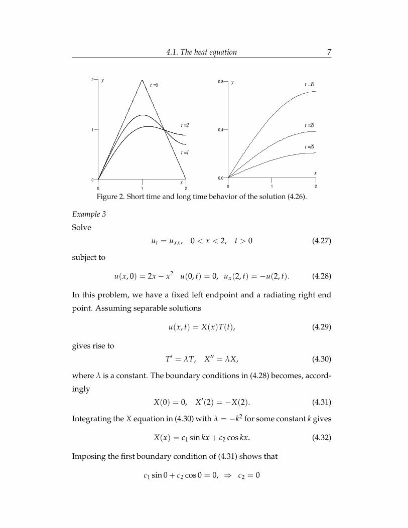
Figure 2 shows the solution both in short time t = 0, 0.1, 0.2 and long time
t = 10, 20, 30.
4.1. The heat equation 7
t = 2
t = 1
t = 0y
x2
0
0
1
2
1
t = 30
t = 20
t = 10y
x
1
0.8
20
0.4
0.0
Figure 2. Short time and long time behavior of the solution (4.26).
Example 3
Solve
ut = uxx, 0 < x < 2, t > 0 (4.27)
subject to
u(x, 0) = 2x− x2 u(0, t) = 0, ux(2, t) = −u(2, t). (4.28)
In this problem, we have a fixed left endpoint and a radiating right end
point. Assuming separable solutions
u(x, t) = X(x)T(t), (4.29)
gives rise to
T′ = λT, X′′ = λX, (4.30)
where λ is a constant. The boundary conditions in (4.28) becomes, accord-
ingly
X(0) = 0, X′(2) = −X(2). (4.31)
Integrating the X equation in (4.30) with λ = −k2 for some constant k gives
X(x) = c1 sin kx + c2 cos kx. (4.32)
Imposing the first boundary condition of (4.31) shows that
c1 sin 0 + c2 cos 0 = 0, ⇒ c2 = 0

8 Chapter 5. Separation of Variables
and the second boundary condition of (4.31) gives
tan 2k = −k. (4.33)
It is very important that we recognize that the solutions of (4.33) are not
equally spaced as seen in earlier problems. In fact, there are an infinite
number of solutions of this equation. Figure 3 shows graphically the curves
y = −k and y = tan 2k. The first three intersection points are the first three
solutions of (4.33).
k
2k
1k
y
k
3
0
2
4
−4
1 2
−2
0 43
Figure 3. The graph of y = tan 2k and y = −k.
Thus, it is necessary that we solve for k numerically. The first 10 solutions
are given in table 1.
n kn n kn1 1.144465 6 8.6966222 2.54349 7 10.2587613 4.048082 8 11.8231624 5.586353 9 13.3890445 7.138177 10 14.955947
Table 1. The first ten solution of tan 2k = −k.
Therefore, we have
X(x) = c1 sin knx. (4.34)
Further, integrating (4.30) for T gives
T(t) = c3e−k2nt (4.35)

4.1. The heat equation 9
and together with X, we have the solution to the PDE as
u(x, t) =∞
∑n=1
cne−k2nt sin knx, (4.36)
Imposing the boundary conditions (4.28) gives
u(0, t) = 2x− x2 =∞
∑n=1
cn sin knx, (4.37)
It is important to know that the cn’s are not given by the formula
cn =22
∫ 2
0(2x− x2)sinknx, dx
as usual. The reason for this is that the kn’s are not equally spaced. So
it is necessary to examine (4.37) on its own. Multiplying by sin kmx and
integrating over [0,2] gives
∫ 2
0(2x− x2) sin kmx dx =
∞
∑n=1
cn
∫ 2
0sin kmx sin knx dx,
For n 6= m, we have∫ 2
0sin kmx sin knx dx =
km sin 2kn cos 2km − kn sin 2km cos 2kn
k2n − k2
m(4.38)
and imposing (4.33) for each of km and kn shows (4.38) to be identically
satisfied. Therefore, we obtain the following when n = m∫ 2
0(2x− x2) sin knx dx = cn
∫ 2
0sin2 knx dx,
or
cn =
∫ 20 (2x− x2) sin knx dx
∫ 20 sin2 knx dx,
(4.39)
Table 2 gives the first ten cn’s that correspond to each kn.
n cn n cn1 0.873214 6 0.0287772 0.341898 7 -.0168033 -.078839 8 0.0153104 0.071427 9 -.0102025 -.032299 10 0.009458
Table 2. The coefficients cn from (4.77).
10 Chapter 5. Separation of Variables
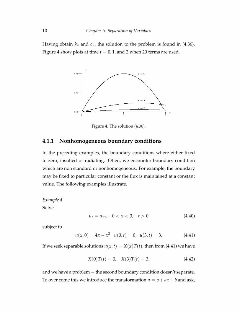
Having obtain kn and cn, the solution to the problem is found in (4.36).
Figure 4 show plots at time t = 0, 1, and 2 when 20 terms are used.
2t =
1t =
0t =
y
x
0 1
0.0
1.0
2
0.5
Figure 4. The solution (4.36).
4.1.1 Nonhomogeneous boundary conditions
In the preceding examples, the boundary conditions where either fixed
to zero, insulted or radiating. Often, we encounter boundary condition
which are non standard or nonhomogeneous. For example, the boundary
may be fixed to particular constant or the flux is maintained at a constant
value. The following examples illustrate.
Example 4
Solve
ut = uxx, 0 < x < 3, t > 0 (4.40)
subject to
u(x, 0) = 4x− x2 u(0, t) = 0, u(3, t) = 3. (4.41)
If we seek separable solutions u(x, t) = X(x)T(t), then from (4.41) we have
X(0)T(t) = 0, X(3)T(t) = 3, (4.42)
and we have a problem− the second boundary condition doesn’t separate.
To over come this we introduce the transformation u = v + ax + b and ask,

4.1. The heat equation 11
”Can we choose the constants a and b as to fix both boundary conditions
to zero. Upon substitution of both boundary conditions (4.41), we obtain
0 = v(0, t) + a(0) + b, 3 = v(3, t) + 3a + b (4.43)
Now we require that v(0, t) = 0 and v(3, t) = 0 which implies that we
must choose a = 1 and b = 0. Therefore, we have
u = v + x. (4.44)
We notice that under the transformation (4.44), the original equation doesn’t
change form, i.e.
ut = uxx ⇒ vt = vxx
however, the initial condition does change, it becomes
v(x, 0) = 3x− x2.
Thus, we have the new problem to solve
vt = vxx, 0 < x < 3, t > 0 (4.45)
subject to
v(x, 0) = 3x− x2 v(0, t) = 0, v(3, t) = 3. (4.46)
At this point, we seek the usual separable solutions V(x, t) = X(x)T(t)
which lead to the and the systems X′′ = −k2X and T′ = −k2T with the
boundary conditions X(0) = 0 and X(3) = 0. Solving for X gives
X(x) = c1 sin kx + c2 cos kx, (4.47)
and imposing both boundary conditions gives
X(x) = c1 sinnπ
3x, (4.48)
and
T(t) = c3e−n2π2
9 t

12 Chapter 5. Separation of Variables
where n is an integer. Therefore, we have the solution of (4.45) as
v(x, t) =∞
∑n=1
bne−n2π2
9 t sinnπ
3x.
Recognizing that we have a Fourier sine series, we obtain the coefficients
bn as
bn =23
∫ 3
0(3x− x2) sin
nπ
3x dx
=[−6(2x− 3)
n2π2 sinnπ
3x +
3(n2π2x2 − 3n2π2x− 18)n3π3 cos
nπ
3x]∣∣∣∣
3
0
=32(1− (−1)n)
n3π3 .
This gives
v(x, t) =32π3
∞
∑n=1
(1− (−1)n)n3 e−
n2π29 t sin
nπ
3x.
and since u = v + x, we obtain the solution for u as
u(x, t) = x +32π3
∞
∑n=1
(1− (−1)n)n3 e−
n2π29 t sin
nπ
3x. (4.49)
2t =
1t =
0t =
y
x
1 2
0
4
2
30
Figure 5. The solution (4.49) at time t = 0, 1 and 2.
Example 5
Solve
ut = uxx, 0 < x < 1, t > 0 (4.50)
subject to
u(x, 0) = 0 ux(0, t) = −1, ux(1, t) = 0. (4.51)

4.1. The heat equation 13
Unfortunately, the trick u = v + ax + b won’t work since ux = vx + a and
choosing a to fix the right boundary to zero only makes the left boundary
nonzero. To overcome this we might try u = v + ax2 + bx but the original
equation changes
ut = uxx, ⇒ vt = vxx + 2a (4.52)
As a second attempt, we try
u = v + a(x2 + 2t) + bx (4.53)
noting now
ut = uxx, ⇒ vt = vxx. (4.54)
Since ux = vx + 2ax + b, then choosing a = 1/2 and b = −1 gives the
the new boundary conditions as vx(0, t) = 0 and vx(2, t) = 0 and the
transformation becomes
u = v +12(x2 + 2t)− x, (4.55)
Finally, we consider the initial condition. From (4.55), we have v(x, 0) =
u(x, 0) − 12 x2 + x = x − x2
2 and our problem is transformed to the new
problem
vt = vxx, 0 < x < 1, t > 0 (4.56)
subject to
v(x, 0) = x− 12
x2, vx(0, t) = vx(1, t) = 0 (4.57)
A separation of variables v = XT leads to X′′ = −k2X and T′ = −k2T
from which we obtain
X = c1 sin kx + c2 cos kx, X = c1k cos kx− c2k sin kx, (4.58)
and imposing the boundary conditions (4.57) gives
c1 = 0, k = nπ, (4.59)
where n is an integer. This then leads to
X(x) = c2 cos nπx (4.60)

14 Chapter 5. Separation of Variables
and further
T(t) = c3e−n2π2t. (4.61)
Finally we arrive at
v(x, t) =a0
2+
∞
∑n=1
ane−n2π2t cos nπx.
noting that we have chosen an = c1c3. Upon substitution of t = 0 and
using the initial condition (4.57), we have
x− 12
x2 =a0
2+
∞
∑n=1
an cos nπx.
a Fourier cosine series. The coefficients are obtained by
a0 =21
∫ 1
0
(x− 1
2x2
), dx = x2 − 1
3x3
∣∣∣∣1
0=
23
,
an =21
∫ 1
0(x− 1
2x2) cos nπx dx
=[−2(x− 1)
n2π2 cos nπx−(
(2x− x2)nπ
+2
n3π3
)sin nπx
]∣∣∣∣1
0
= − 2n2π2 .
Thus, we obtain the solution for v as
v(x, t) =13− 2
π2
∞
∑n=1
1n2 e−n2π2t cos nπx.
and this, together with the transformation (4.55) gives
u(x, t) =12(x2 + 2t)− x +
13− 2
π2
∞
∑n=1
1n2 e−n2π2t cos nπx. (4.62)
Figure 6 shows plots at time t = 0.01, 0.5, 1.0 and 1.5. It is interesting to
note that at the left boundary ux = −1 and since the flux φ = −kux implies
that φ = k > 0 which gives that the flux is position and that heat is being
added at the left boundary. Hence the profile increase at the left while
insulated at the right boundary (no flux).

4.1. The heat equation 15
1.5t =
1.0t =
0.5t =
0.1t =
y
x
1.00.0 0.5
1
2
0
Figure 6. The solution (4.62) at time t = 0, 1 and 2.
A natural question is, can we transform
ut = uxx, 0 < x < L, t > 0, (4.63)
u(x, 0) = f (x), u(0, t) = p(t), u(L, t) = q(t) (4.64)
to a problem with standard boundary conditions. The answer is yes. We
seek a transformation of the form
u = v + A(t)x + B(t) (4.65)
as to transform the nonstandard boundary conditions to standard ones.
On substitution of the u and v boundary conditions, we obtain
p(t) = 0 + A(t)0 + B(t), q(t) = 0 + A(t)L + B(t) (4.66)
and solving for A(t) and B(t) gives
A(t) =q(t)− p(t)
L, B(t) = p(t), (4.67)
which results in the transformation
u = v +q(t)− p(t)
Lx + p(t)
= v + q(t)xL
+ p(t)(L− x)
L. (4.68)
However in doing so, we change not only the original equation but also
the initial condition. They becomes, respectively
vt = vxx − q′(t)xL
+ p′(t)(L− x)
L,
v(x, 0) = f (x)− q(0)xL− p(0)
(L− x)L
.

16 Chapter 5. Separation of Variables
The new initial condition doesn’t pose a problem but how do we solve the
heat equation with a term added to the equation.
4.1.2 Nonhomogeneous equations
We now focus our attention to solving the heat equation with a source
term
ut = uxx + Q(x), 0 < x < L, t > 0, (4.69)
u(0, t) = 0, u(L, t) = 0, u(x, 0) = f (x).
To investigate this problem, we will considered a particular example where
L = 2, f (x) = 2x − x2 and Q(x) = 1− |x − 1|. If we were to consider this
problem without a source term we would have solutions of the form
u(x, t) =∞
∑n=1
Tn(t) sinnπx
2, (4.70)
where
Tn(t) =16(1− (−1)n)
n3π3 e−n2π2
4 t (4.71)
We note that even if this Tn wasn’t known, we could find it as substitution
of (4.70) into the heat equation and isolating coefficients of sin nπx2 , would
lead to
T′n(t) = −n2π2
4Tn(t),
leading to the solution (4.71). For the problem with a source term we look
for solutions of the same form i.e. (4.70). However, in order that this tech-
nique works, it is necessary to expand the source term also in terms of a
Fourier sine series, i.e.
Q(x) =∞
∑n=1
qn sinnπx
2. (4.72)
For
Q(x) =
{x if 0 < x < 1,2− x if 1 < x < 2,
(4.73)

4.1. The heat equation 17
where
qn =∫ 2
0Q(x) sin
nπx2
dx.
=∫ 1
0x sin
nπx2
dx +∫ 2
x(2− x) sin
nπx2
dx,
=[
4n2π2 sin
nπx2
− 2xnπ cosnπx
2
]∣∣∣∣1
0
+[− 4
n2π2 sinnπx
2+
2x4
nπcos
nπx2
]∣∣∣∣2
1,
=8
n2π2 sinnπx
2. (4.74)
Substituting both (4.70) and (4.72) into (4.69) gives
∞
∑n=1
T′n(t) sinnπx
2=
∞
∑n=1
−(nπx
2
)2Tn(t) sin
nπx2
+∞
∑n=1
qn sinnπx
2,
and re-grouping and isolating the coefficients of sin nπx2 gives
T′n(t) +n2π2
4Tn(t) = qn, (4.75)
a linear ODE in Tn(t)! On solving (4.75) we obtain
Tn(t) =4
n2π2 qn + bne−( nπ2 )2t,
giving the final solution
u(x, t) =∞
∑n=1
(4
n2π2 qn + bne−( nπ2 )2t
)sin
nπx2
. (4.76)
Imposing the initial condition gives (4.70)
2x− x2 =∞
∑n=1
(4
n2π2 qn + bn
)sin
nπx2
.
If we set
cn =4
n2π2 qn + bn,
then we have
2x− x2 =∞
∑n=1
cn sinnπx
2.

18 Chapter 5. Separation of Variables
a regular Fourier sine series. Therefore
cn =∫ 2
0
(2x− x2
)sin
nπx2
dx.
=16
n3π3
(1− cos
nπ
2
), (4.77)
which in turn, gives
bn = cn − 4n2π2 qn,
and finally, the solution as
u(x, t) =∞
∑n=1
(4
n2π2 qn +(
cn − 4n2π2 qn
)e−( nπ
2 )2t)
sinnπx
2, (4.78)
where qn and cn are given in (4.74) and (4.77), respectively. Typical plots
are given in figure 7 at times t = 0, 1, 2 and 3.
3t =
2t =
1t =
0t =y
x
20 1
0.5
1.0
0.0
Figure 7. The solution (4.78) at time t = 0, 1, 2 and 3.
It is interesting to note that if we let t → ∞ the solution approaches the
same curve at t = 3. This is what is called steady state (no changes in
time). It is natural to ask “Can we find this steady state solution.?” The
answer is yes. For the steady state, ut → 0 as t → ∞ and the original PDE
becomes
uxx + Q(x) = 0. (4.79)
Integrating twice with Q(x) given in (4.73) gives
u =
{− x3
6 + c1x + c2 if 0 < x < 1,x3
6 − x2 + k1x + k2 if 1 < x < 2,(4.80)

4.1. The heat equation 19
where c1, c2, k1 and k2 are constants of integration. Imposing that the solu-
tion and its first derivative are continuous at x = 1 and that the solution is
zer0 at the endpoints gives
c1 − c1 + 1 = 0, c1 + c2 − k1 − k2 +23
= 0,
c2 = 0, 2k1 + k2 − 83
= 0,
which gives, upon solving
c1 =12
, c2 = 0, k1 =32
, k2 = −13
(4.81)
This, in turn gives the steady state solution as
u =
{− x3
6 + x2 if 0 < x < 1,
x3
6 − x2 + 3x2 − 1
3 if 1 < x < 2.(4.82)
4.1.3 Equations with a solution dependent source term
We now consider the heat equation with a solution dependent source term.
For simplicity we will consider a source term that is linear. Take, for ex-
ample
ut = uxx + αu, 0 < x < 1, t > 0,
u(0, t) = 0, u(1, t) = 0, u(x, 0) = x− x2, (4.83)
where α is some constant. We could try a separation of variables to ob-
tain solutions for this problem, but for more complicated source terms like
Q(x, t)u, a separation of variables is unsuccessful. Therefore, we try a dif-
ferent technique. Here we will try and transform the PDE to one that has
no source term. In attempting to do so, we seek a transformation of the
form
u(x, t) = A(x, t)v (4.84)
and ask “Is is possible to find A such that the source term in (4.83) can be
removed?” Substituting of (4.84) in (4.83) gives
Avt + Atv = Avxx + 2Axvx + Axxv + αAv,
20 Chapter 5. Separation of Variables
and dividing by A and expanding and regrouping gives
vt = vxx + 2Ax
Avx +
(Axx
A− At
A+ α
)v.
In order to target the standard heat equation, we choose
Ax = 0,Axx
A− At
A+ α = 0. (4.85)
From the first we obtain that A = A(t) and from the second we obtain
A′ = αA which has the solution A(t) = A0eαt for some constant A0. The
boundary conditions becomes
u(0, t) = 0 ⇒ A0eαtv(0, t) = 0 ⇒ v(0, t) = 0,
v(1, t) = 0 ⇒ A0eαtv(1, t) = 0 ⇒ v(1, t) = 0,
so the boundary conditions become unchanged. Next, we consider the
initial condition, so
u(x, 0) = x− x2 ⇒ A0eα0v(x, 0) = 0 ⇒ A0v(x, 0) = x− x2,
and as to leave the initial condition unchanged, we choose A0 = 1. Thus,
under the transformation
u = eαtv (4.86)
the problem (4.83) becomes
vt = vxx, 0 < x < 1, t > 0,
v(x, 0) = 0, v(1, t) = 0, v(x, 0) = x− x2, (4.87)
This particular problem was considered at the beginning of this chapter,
(4.1) where the solution was given in (4.26), namely
v(x, t) =4
π3
∞
∑n=1
1− (−1)n
n3 e−n2π2t sin nπx,
and so, from (4.86) we obtain the solution of (4.83) as
u(x, t) =4
π3 eαt∞
∑n=1
1− (−1)n
n3 e−n2π2t sin nπx. (4.88)

4.1. The heat equation 21
Figure 8 shows plots at times t = 0, 0.1 and 0.2 when α = 5 and 12. It
is interesting to note that in the case where α = 5, the diffusion is slower
in comparison with no source term (i.e α = 0 see Figure 1) and there is no
diffusion at all when α = 12.
0.2t =
0.1t =
0t =
x
0.5
0.0
0.3
0.1
0.2
0.0 1.0
0.2t =
0.1t =
0t =
y
x
0.0 0.5
0.0
0.4
1.0
0.2
Figure 8. The solution (4.88) of the heat equation with a source (4.83) with α = 5and α = 12.
It is natural to ask, for what value of α do we achieve a steady state
solution. To answer this consider the first few terms of the solution (4.88)
u =8
π3 eαt(
e−π2t sin πx +127
e−9π2t sin 3πx + . . .)
. (4.89)
Now clearly the exponential terms in (·) will decay to zero with the first
term decaying the slowest. Therefore, it is the balance between eαt and
e−π2t which determine whether the solution will decay to zero or not. It is
equality α = π2 that gives the steady state solution.
Example 6
Solve
ut = uxx + αu, 0 < x < 2, t > 0
u(x, 0) = 4x− x3 ux(0, t) = 0, ux(2, t) = 0. (4.90)
Established already is that the transformation (4.86) will transform the
equation to the heat equation and will leave the initial condition unchanged.

22 Chapter 5. Separation of Variables
It is now necessary to determine what happens to the boundary condi-
tions. Using (4.86) we have
ux(0, t) = 0 ⇒ A0eαtvx(0, t) = 0 ⇒ vx(0, t) = 0, (4.91)
vx(2, t) = 0 ⇒ A0eαtvx(2, t) = 0 ⇒ vx(2, t) = 0, (4.92)
and so the insulted boundary conditions also remain insulated! Thus, the
problem (4.90) becomes
vt = vxx, 0 < x < 2, t > 0
v(x, 0) = 4x− x2, vx(0, t) = 0, vx(2, t) = 0. (4.93)
Using a separation of variables and imposing the boundary conditions
gives (see example 1)
v =12
a0 +∞
∑n=1
ane−n2π2
4 t cosnπ
2x, (4.94)
where
a0 =22
∫ 2
0(4x− x3) dx =
[2x2 − x4
4
]∣∣∣∣2
0= 4,
an =22
∫ 2
0(4x− x3) cos
nπ
2x dx (4.95)
=[(
2(4x− x3)nπ
+48
n3π3
)sin
nπ
2x +
(4(4− 3x2)
n2π2 +96
n4π4
)cos
nπ
2x]∣∣∣∣
2
0
= − 16n2π2 −
96n4π4 +
(6
nπ+
48n3π3
)sin
nπ
2+
(4
n2π2 +96
n4π4
)cos
nπ
2.
Together with the transformation (4.86), the solution of (4.90) is
u = 2eαt + eαt∞
∑n=1
ane−n2π2
4 t cosnπ
2x, (4.96)
where an is given in (4.95). Figure 9 show plots at t = 0, 0.2, 0.4 and 0.6
when α = −2 and 2. It is interesting to note that the sign of α will deter-
mine whether the solution will grow or decay exponentially.

4.1. The heat equation 23
0.6t =
0.4t =
0.2t =
0t =
y
x
2
2
3
10
1
0
0.6t =
0.4t =
0.2t =
0t =
y
x
0
6
21
0
2
4
8
Figure 9. The solution (4.96) of the heat equation with a source (4.90) with noflux boundary condition with α = −2 and α = 2.
4.1.4 Equations with a solution dependent convective term
We now consider the heat equation with a solution dependent linear con-
vection term, i.e.
ut = uxx + β ux, 0 < x < 1, t > 0
u(0, t) = 0, u(1, t) = 0, u(x, 0) = x− x2, (4.97)
where β is some constant. We consider the same initial and boundary
conditions as in the previous section as it provides a means of comparing
the two respective problems. Again, we could try a separation of variables
to obtain solutions for this problem, but for more complicated convection
terms like P(x, t)ux, a separation of variable is unsuccessful. Therefore,
we again try a different technique. We will try and transform the PDE
to one that has no convection term. In attempting to do so, we seek a
transformation of the form
u(x, t) = A(x, t)v (4.98)
and ask “Is is possible to find A such that the convection term can be re-
moved?” Substituting of (4.98) in (4.97) gives
Avt + Atv = Avxx + 2Axvx + Axxv + β (Avx + Axv) ,

24 Chapter 5. Separation of Variables
and dividing by A and expanding and regrouping gives
vt = vxx +2Ax + βA
Avx +
Axx − At + βAx
Av. (4.99)
In order to target the standard heat equation, we choose
2Ax + βA = 0, Axx − At + βAx = 0. (4.100)
From the first we obtain that A(x, t) = C(t)e−12 βx and from the second
we obtain C′ + β2
4 C = 0 which has the solution C(t) = A0e−14 β2t for some
constant A0. This then gives
A(x, t) = A0e−12 βx− 1
4 β2t (4.101)
The boundary conditions becomes
u(0, t) = 0 ⇒ C0e−14 β2tv(0, t) = 0 ⇒ v(0, t) = 0, (4.102)
v(1, t) = 0 ⇒ C0e−12− 1
4 β2tv(1, t) = 0 ⇒ v(1, t) = 0, (4.103)
so the boundary conditions become unchanged. Next, we consider the
initial condition, so
u(x, 0) = x− x2 ⇒ v(x, 0) = (x− x2)e12 βx, (4.104)
where we have chosen A0 = 1. So here, the initial condition actually
changes. Thus, under the transformation
u = e−12 βx− 1
4 β2tv, (4.105)
the problem (4.97) becomes
vt = vxx, 0 < x < 1, t > 0,
v(x, 0) = 0, v(1, t) = 0, v(x, 0) = (x− x2)e12 βx. (4.106)
As in the previous section, the solution is given by
v(x, t) =∞
∑n=1
bne−n2π2t sin nπx, (4.107)

4.1. The heat equation 25
where bn is now given by
bn =21
∫ 1
0(x− x2)e
12 βx sin nπx dx, (4.108)
and from (4.105)
u(x, t) = e−12 βx− 1
4 β2t∞
∑n=1
bne−n2π2t sin nπx, (4.109)
At this point we consider two particular examples: β = 6 and β = −12.
For β = 6
bn = 2∫ 1
0(x− x2)e3x sin nπx dx
= −4nπ27 + n2π2 + 2n2π2e3 cos nπ
(9 + n2π2)3 . (4.110)
For β = −12
bn = 2∫ 1
0(x− x2)e−6x sin nπx dx
= 2nπ7n2π2 + 108 + (5n2π2 + 324)e−6 cos nπ
(36 + n2π2)3 . (4.111)
The respective solutions for each are
u(x, t) = 4πe−12 βx− 1
4 β2t (4.112)
×∞
∑n=1
n27 + n2π2 + 2n2π2e3 cos nπ
(9 + n2π2)3 e−n2π2t sin nπx,
u(x, t) = 2πe−12 βx− 1
4 β2t (4.113)
×∞
∑n=1
n7n2π2 + 108 + (5n2π2 + 324)e−6 cos nπ
(36 + n2π2)3 e−n2π2t sin nπx.
Figure 10 shows graphs at a variety of times for β = 6 and β = −12.

26 Chapter 5. Separation of Variables
0.1t =
0.05t =
0t =
y
x
0.0 0.5 1.0
0.3
0.1
0.0
0.2
0.05t =
0.025t =
0t =
y
x
0.0 0.5 1.0
0.3
0.1
0.0
0.2
Figure 10. The solution (4.112) of the heat equation with convection with fixedboundary conditions with β = 6 and β = −12.
Example 7
As a final example, we consider
ut = uxx + βux, 0 < x < 2, t > 0 (4.114)
subject to
u(x, 0) = 4x− x3 ux(0, t) = 0, ux(2, t) = 0. (4.115)
This problem is like problem 6 but with insulated boundary conditions.
Here, we will simply transform the problem to one that is in standard form
as to contrast the differences between the two problems. The transforma-
tion (4.105) transforms (4.114) to the heat equation so we will primarily fo-
cus on the boundary and initial conditions. For the boundary conditions,
upon differentiating (4.105) with respect to x gives
ux = e−12 βx− 1
4 β2tvx − β
2e−
12 βx− 1
4 β2tv, (4.116)
and so
ux(0, t) = 0 ⇒ vx(0, t)− β
2v(0, t) = 0, (4.117)
ux(2, t) = 0 ⇒ vx(2, t)− β
2v(2, t) = 0. (4.118)

4.2. Laplace’s equation 27
Thus, the insulated boundary condition become radiating boundary con-
ditions. As for the initial condition
u(x, 0) = 4x− x3 ⇒ v(x, 0) = (4x− x3)e12 βx, (4.119)
so again, the initial condition changes.
4.2 Laplace’s equation
The two dimensional Laplace’s equation is
uxx + uyy = 0 (4.120)
We will show that a separation of variables also works for this equation
As an example consider the boundary conditions
u(x, 0) = 0, u(x, 1) = x− x2 (4.121a)
u(0, y) = 0, u(1, 0) = 0. (4.121b)
If we assume separable solutions of the form
u(x, y) = X(x)Y(y), (4.122)
then substituting this into (4.120) gives
X′′Y + XY′′ = 0. (4.123)
Dividing by XY and expanding gives
X′′
X+
Y′′
Y= 0, (4.124)
and since each term is only a function of x or y, then each must be constant
givingX′′
X= λ,
Y′′
Y= −λ. (4.125)
From the first of (4.121a) and both of (4.121b) we deduce the boundary
conditions
X(0) = 0, X(1) = 0, Y(0) = 0. (4.126)
28 Chapter 5. Separation of Variables
The remaining boundary condition in (4.121a) will be used later. As seen
the in previous section, in order to solve the X equation in (4.125) subject
to the boundary conditions (4.126), it is necessary to set λ = −k2. The X
equation (4.125) as the general solution
X = c1 sin kx + c2 cos kx (4.127)
To satisfy the boundary conditions in (4.126) it is necessary to have c2 = 0
and k = nπ, k ∈ Z+ so
X(x) = c1 sin nπx. (4.128)
From (4.125), we obtain the solution to the Y equation
Y(y) = c3 sinh nπy + c4 cosh nπy (4.129)
Since Y(0) = 0 this implies c4 = 0 so
X(x)Y(y) = an sin nπx sinh nπy (4.130)
where we have chosen an = c1c3. Therefore, we obtain the solution to
(4.120) subject to three of the four boundary conditions in (4.121)
u =∞
∑n=1
an sin nπx sinh nπy. (4.131)
The remaining boundary condition is (4.121a) now needs to be satisfied,
thus
u(x, 1) = x− x2 =∞
∑n=1
an sin nπx sinh nπ. (4.132)
This looks like a Fourier sine series and if we let An = an sinh nπ, this
becomes∞
∑n=1
An sin nπx = x− x2. (4.133)
which is precisely a Fourier sine series. The coefficients An are given by
An =21
∫ 2
0
(x− x2
)sin nπx dx
=16
n3π3 (1− cos nπ), (4.134)

4.2. Laplace’s equation 29
and since An = an sinh nπ, this gives
an =4(1− (−1)n)n3π3 sinh nπ
. (4.135)
Thus, the solution to Laplace’s equation with the boundary conditions
given in (4.121) is
u(x, y) =4
π3
∞
∑n=1
1− (−1)n
n3 sin nπxsinh nπysinh nπ
. (4.136)
Figure 11 show both a top view and a 3− D view of the solution.
0.001u =
y
x
0.2u =
0.1u =
0.05u =
0.025u =
1.0
0.5
0.0
1.00.0 0.5
0.0
0.1
0.2
0.5
u
1.0
y
1.0
x
Figure 11. The solution (4.120) with the boundary conditions (4.121)
In general, using separation of variables, the solution of
uxx + uyy = 0, 0 < x < Lx, 0 < y < Ly, (4.137)
subject to
u(x, 0) = 0, u(x, 1) = f (x),
u(0, y) = 0, u(1, y) = 0,
is
u =∞
∑n=1
bn sinnπxLx
sinh nπyLy
sinh nπLy
, (4.139)

30 Chapter 5. Separation of Variables
where
bn =2Lx
∫ Lx
0f (x) sin
nπxLx
dx. (4.140)
In the next three examples, we will construct solutions of Laplace’s equa-
tion when we have nonzero boundary condition on each of the remaining
three sides of the region 0 < 1, 0 < y < 1.
Example 8
Solve
uxx + uyy = 0, (4.141)
subject to
u(x, 0) = 0, u(x, 1) = 0, (4.142a)
u(0, y) = 0, u(1, y) = y− y2. (4.142b)
Assume separable solutions of the form
u(x, y) = X(x)Y(y) (4.143)
Then substituting this into (4.141) gives
X′′Y + XY′′ = 0. (4.144)
Dividing by XY and expanding gives
X′′
X+
Y′′
Y= 0, (4.145)
from which we obtain
X′′
X= λ,
Y′′
Y= −λ (4.146)
From (4.186) we deduce the boundary conditions
X(0) = 0, Y(0) = 0, Y(1) = 0. (4.147)

4.2. Laplace’s equation 31
The remaining boundary condition in (4.186) will be used later. As seen
the in previous problem, in order to solve the Y equation in (4.146) subject
to the boundary conditions (4.147), it is necessary to set λ = k2. The Y
equation (4.146) as the general solution
Y = c1 sin ky + c2 cos ky (4.148)
To satisfy the boundary conditions in (4.147) it is necessary to have c2 = 0
and k = nπ so
Y(y) = c1 sin nπy. (4.149)
From (4.146), we obtain the solution to the X equation
X(x) = c3 sinh nπx + c4 cosh nπx (4.150)
Since X(0) = 0 this implies c4 = 0. This gives
X(x)Y(y) = an sinh nπx sin nπy (4.151)
where we have chosen an = c1c3. Therefore, we obtain
u =∞
∑n=1
an sinh nπx sin nπy. (4.152)
The remaining boundary condition is (4.186) now needs to be satisfied,
thus
u(1, y) = y− y2 =∞
∑n=1
an sinh nπ sin nπy. (4.153)
If we let An = an sinh nπ, this becomes
∞
∑n=1
An sin nπy = y− y2. (4.154)
Comparing with previous problem, we find that interchanging x and y
interchanges the two problems and thus we con conclude that
An =16
n3π3 (1− cos nπ), (4.155)

32 Chapter 5. Separation of Variables
and further that the solution to Laplace’s equation with the boundary con-
ditions given in (4.141) subject to (4.186) is
u =4
π3
∞
∑n=1
1− (−1)n
n3sinh nπxsinh nπ
sin nπy. (4.156)
Figure 12 show both a top view and a 3− D view of the solution. In com-
paring the solutions (4.136) and (4.156) shows that if we interchange x and
y they are the same. This should not be surprising because if we con-
sider Laplace equations with the boundary conditions given in (4.121) and
(4.186), that if we interchange x and y, the problems are transformed to
each other.
In general, using separation of variables, the solution of
uxx + uyy = 0, 0 < x < Lx, 0 < y < Ly (4.157)
subject to
u(x, 0) = 0, u(x, 1) = 0
u(0, y) = 0, u(1, y) = g(y).
is
u =∞
∑n=1
bnsinh nπx
Lx
sinh nπLx
sinnπyLy
(4.159)
where
bn =2Ly
∫ Ly
0g(y) sin
nπyLy
dy (4.160)
Example 9
Solve
uxx + uyy = 0 (4.161)
subject to
u(x, 0) = x− x2, u(x, 1) = 0 (4.162a)
u(0, y) = 0, u(1, y) = 0. (4.162b)

4.2. Laplace’s equation 33
Again, assuming separable solutions of the form
u(x, y) = X(x)Y(y) (4.163)
leads to
X′′Y + XY′′ = 0, (4.164)
when substituted into (4.161). Dividing by XY and expanding gives
X′′
X+
Y′′
Y= 0. (4.165)
Since each term is only a function of x or y then each must be constant
givingX′′
X= λ,
Y′′
Y= −λ (4.166)
From the first of (4.162a) and both of (4.162b) we deduce the boundary
conditions
X(0) = 0, X(1) = 0, Y(1) = 0, (4.167)
noting that the last boundary condition is different than the boundary con-
dition considered at the beginning of this section (i.e. Y(0) = 0). The re-
maining boundary condition in (4.162a) will be used later. In order to solve
the X equation in (4.166) subject to the boundary conditions (4.167), it is
necessary to set λ = −k2. The X equation (4.166) as the general solution
Y = c1 sin kx + c2 cos kx (4.168)
To satisfy the boundary conditions in (4.167) it is necessary to have c2 = 0
and k = nπ so
X(x) = c1 sin nπx. (4.169)
From (4.166), we obtain the solution to the Y equation
Y(y) = c3 sinh nπy + c4 cosh nπy (4.170)
Since Y(1) = 0 this implies
c3 sinh nπ + c4 cosh nπ = 0 ⇒ c4 = −c2sinh nπ
cosh nπ. (4.171)

34 Chapter 5. Separation of Variables
From (4.172) we have
Y(y) = c3 sinh nπy− c3 cosh nπysinh nπ
cosh nπ
= −c3sinh nπ(1− y)
sinh nπ. (4.172)
so
X(x)Y(y) = an sin nπx sinh nπ(1− y) (4.173)
where we have chosen an = −c1c3/ sinh nπ. Therefore, we obtain
u =∞
∑n=1
an sin nπx sinh nπ(1− y). (4.174)
The remaining boundary condition is (4.162a) now needs to be satisfied,
thus
u(x, 0) = x− x2 =∞
∑n=1
an sin nπx sinh nπ. (4.175)
At this point we recognize that this problem is now identically to the first
problem in this section where we obtained
an =4(1− (−1)n)n3π3 sinh nπ
(4.176)
so the solution to Laplace’s equation with the boundary conditions given
in (4.179) is
u(x, y) =4
π3
∞
∑n=1
1− (−1)n
n3 sin nπxsinh nπ(1− y)
sinh nπ. (4.177)
Figure 12 show both a top view and a 3− D view of the solution.
In general, using separation of variables, the solution of
uxx + uyy = 0, 0 < x < Lx, 0 < y < Ly (4.178)
subject to
u(x, 0) = f (x), u(x, 1) = 0
u(0, y) = 0, u(1, y) = 0.

4.2. Laplace’s equation 35
is
u =∞
∑n=1
bn sinnπxLx
sinh nπ(1−y)Ly
sinh nπLy
(4.180)
where
bn =2Lx
∫ Lx
0f (x) sin
nπxLx
dx (4.181)
Example 10
As the final example, we consider
uxx + uyy = 0 (4.182)
subject to
u(x, 0) = 0, u(x, 1) = 0 (4.183a)
u(0, y) = y− y2, u(1, y) = 0. (4.183b)
We could go through a separation of variables to obtain the solution but
we can avoid many of the steps by considering the previous three prob-
lems. One will notice to transform between the first and second problem,
the variables x and y only need to be interchanged. This can also be seen in
their respective solutions. One will also notice to transform between this
problem and problem 9, we only need to transform x and y again. Thus,
to obtain the solution for this final problem, we will transform the solution
given in (4.177) giving
u(x, y) =4
π3
∞
∑n=1
1− (−1)n
n3sinh nπ(1− x)
sinh nπsin nπy. (4.184)
In general, using separation of variables, the solution of
uxx + uyy = 0, 0 < x < Lx, 0 < y < Ly (4.185)
subject to
u(x, 0) = 0, u(x, 1) = 0
u(0, y) = g(y), u(1, y) = 0.

36 Chapter 5. Separation of Variables
is
u =∞
∑n=1
bnsinh nπ(1−x)
Ly
sinh nπLy
sinnπyLy
. (4.187)
where
bn =2Ly
∫ Ly
0g(y) sin
nπyLy
dy (4.188)