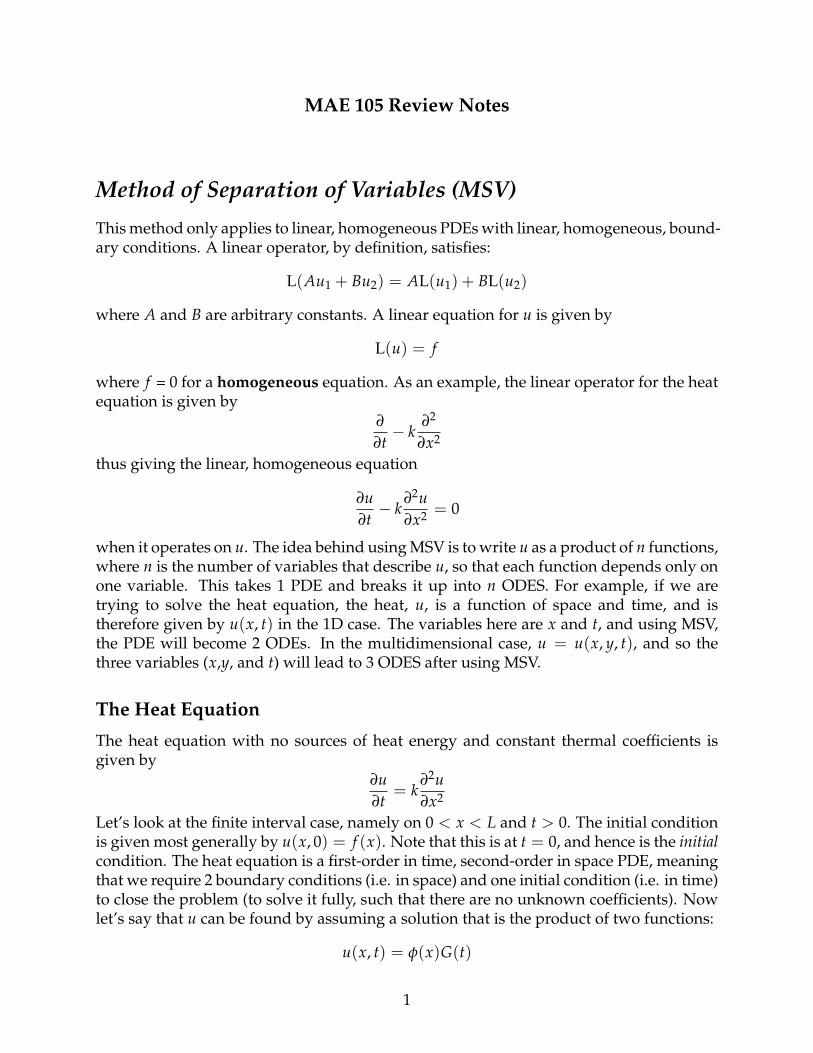
MAE 105 Review Notes

Method of Separation of Variables (MSV)

This method only applies to linear, homogeneous PDEs with linear, homogeneous, bound-ary conditions. A linear operator, by definition, satisfies:

L(Au1 + Bu2) = AL(u1) + BL(u2)

where A and B are arbitrary constants. A linear equation for u is given by

L(u) = f

where f = 0 for a homogeneous equation. As an example, the linear operator for the heatequation is given by

∂

∂t− k

∂2

∂x2

thus giving the linear, homogeneous equation

∂u∂t− k

∂2u∂x2 = 0

when it operates on u. The idea behind using MSV is to write u as a product of n functions,where n is the number of variables that describe u, so that each function depends only onone variable. This takes 1 PDE and breaks it up into n ODES. For example, if we aretrying to solve the heat equation, the heat, u, is a function of space and time, and istherefore given by u(x, t) in the 1D case. The variables here are x and t, and using MSV,the PDE will become 2 ODEs. In the multidimensional case, u = u(x, y, t), and so thethree variables (x,y, and t) will lead to 3 ODES after using MSV.

The Heat Equation

The heat equation with no sources of heat energy and constant thermal coefficients isgiven by

∂u∂t

= k∂2u∂x2

Let’s look at the finite interval case, namely on 0 < x < L and t > 0. The initial conditionis given most generally by u(x, 0) = f (x). Note that this is at t = 0, and hence is the initialcondition. The heat equation is a first-order in time, second-order in space PDE, meaningthat we require 2 boundary conditions (i.e. in space) and one initial condition (i.e. in time)to close the problem (to solve it fully, such that there are no unknown coefficients). Nowlet’s say that u can be found by assuming a solution that is the product of two functions:

u(x, t) = φ(x)G(t)

1

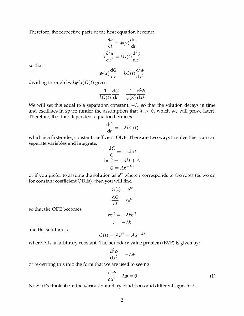
Therefore, the respective parts of the heat equation become:

∂u∂t

= φ(x)dGdt

k∂2u∂x2 = kG(t)

d2φ

dx2

so that

φ(x)dGdt

= kG(t)d2φ

dx2

dividing through by kφ(x)G(t) gives

1kG(t)

dGdt

=1

φ(x)d2φ

dx2

We will set this equal to a separation constant, −λ, so that the solution decays in timeand oscillates in space (under the assumption that λ > 0, which we will prove later).Therefore, the time-dependent equation becomes

dGdt

= −λkG(t)

which is a first-order, constant coefficient ODE. There are two ways to solve this: you canseparate variables and integrate:

dGG

= −λkdt

ln G = −λkt + AG = Ae−λkt

or if you prefer to assume the solution as ert where r corresponds to the roots (as we dofor constant coefficient ODEs), then you will find

G(t) = ert

dGdt

= rert

so that the ODE becomesrert = −λkert

r = −λkand the solution is

G(t) = Aert = Ae−λkt

where A is an arbitrary constant. The boundary value problem (BVP) is given by:

d2φ

dx2 = −λφ

or re-writing this into the form that we are used to seeing,

d2φ

dx2 + λφ = 0 (1)

Now let’s think about the various boundary conditions and different signs of λ.

2

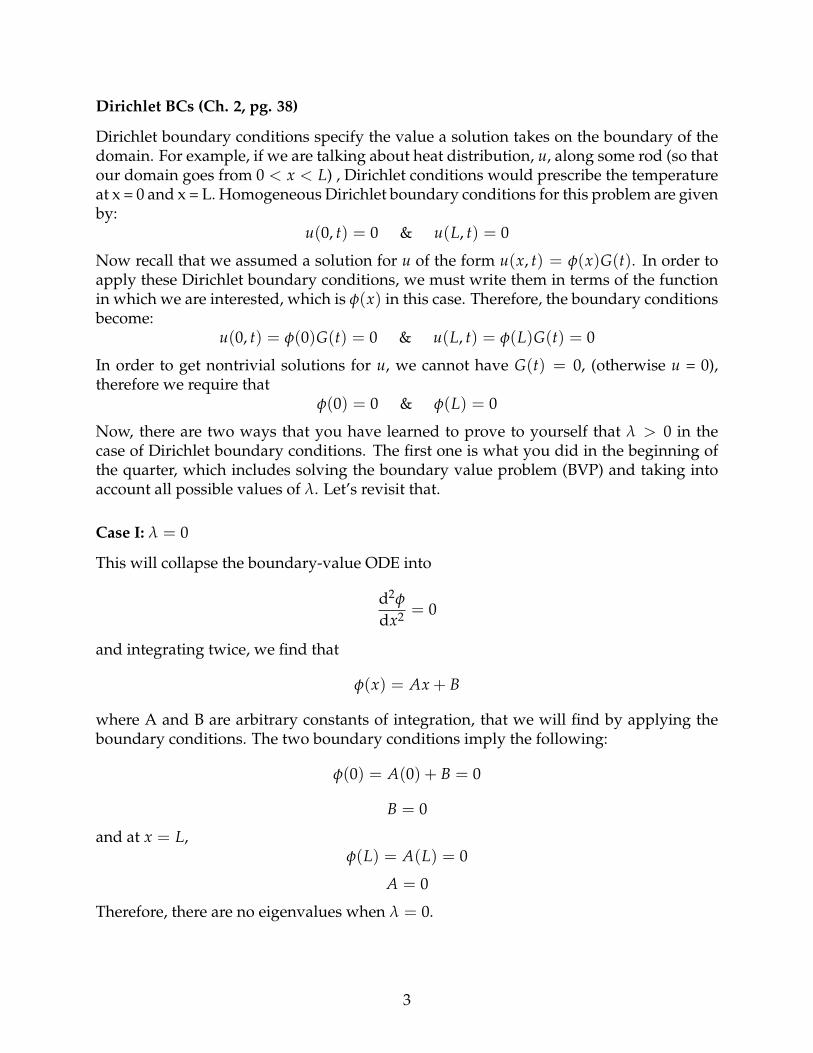
Dirichlet BCs (Ch. 2, pg. 38)

Dirichlet boundary conditions specify the value a solution takes on the boundary of thedomain. For example, if we are talking about heat distribution, u, along some rod (so thatour domain goes from 0 < x < L) , Dirichlet conditions would prescribe the temperatureat x = 0 and x = L. Homogeneous Dirichlet boundary conditions for this problem are givenby:

u(0, t) = 0 & u(L, t) = 0

Now recall that we assumed a solution for u of the form u(x, t) = φ(x)G(t). In order toapply these Dirichlet boundary conditions, we must write them in terms of the functionin which we are interested, which is φ(x) in this case. Therefore, the boundary conditionsbecome:

u(0, t) = φ(0)G(t) = 0 & u(L, t) = φ(L)G(t) = 0

In order to get nontrivial solutions for u, we cannot have G(t) = 0, (otherwise u = 0),therefore we require that

φ(0) = 0 & φ(L) = 0

Now, there are two ways that you have learned to prove to yourself that λ > 0 in thecase of Dirichlet boundary conditions. The first one is what you did in the beginning ofthe quarter, which includes solving the boundary value problem (BVP) and taking intoaccount all possible values of λ. Let’s revisit that.

Case I: λ = 0

This will collapse the boundary-value ODE into

d2φ

dx2 = 0

and integrating twice, we find that

φ(x) = Ax + B

where A and B are arbitrary constants of integration, that we will find by applying theboundary conditions. The two boundary conditions imply the following:

φ(0) = A(0) + B = 0

B = 0

and at x = L,φ(L) = A(L) = 0

A = 0

Therefore, there are no eigenvalues when λ = 0.

3

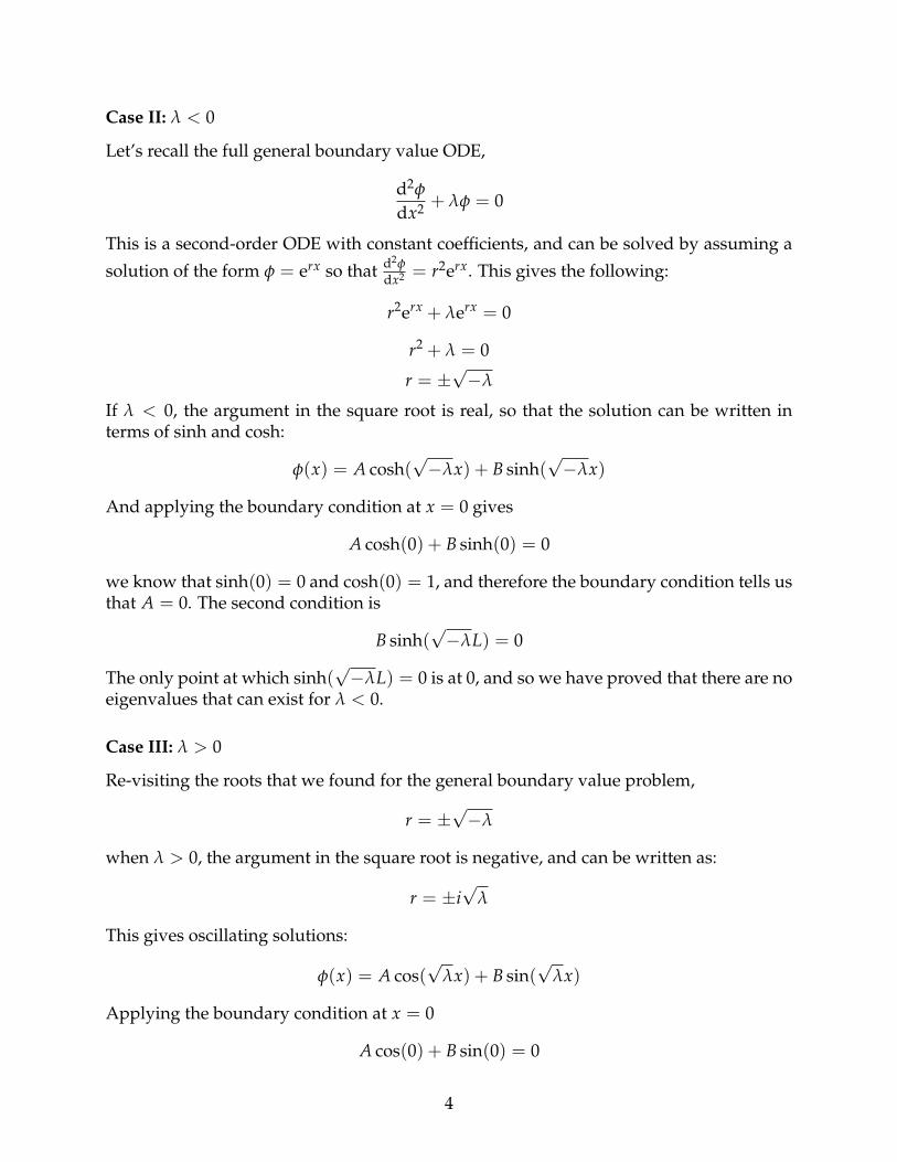
Case II: λ < 0

Let’s recall the full general boundary value ODE,

d2φ

dx2 + λφ = 0

This is a second-order ODE with constant coefficients, and can be solved by assuming a

solution of the form φ = erx so that d2φdx2 = r2erx. This gives the following:

r2erx + λerx = 0

r2 + λ = 0

r = ±√−λ

If λ < 0, the argument in the square root is real, so that the solution can be written interms of sinh and cosh:

φ(x) = A cosh(√−λx) + B sinh(

√−λx)

And applying the boundary condition at x = 0 gives

A cosh(0) + B sinh(0) = 0

we know that sinh(0) = 0 and cosh(0) = 1, and therefore the boundary condition tells usthat A = 0. The second condition is

B sinh(√−λL) = 0

The only point at which sinh(√−λL) = 0 is at 0, and so we have proved that there are no

eigenvalues that can exist for λ < 0.

Case III: λ > 0

Re-visiting the roots that we found for the general boundary value problem,

r = ±√−λ

when λ > 0, the argument in the square root is negative, and can be written as:

r = ±i√

λ

This gives oscillating solutions:

φ(x) = A cos(√

λx) + B sin(√

λx)

Applying the boundary condition at x = 0

A cos(0) + B sin(0) = 0

4

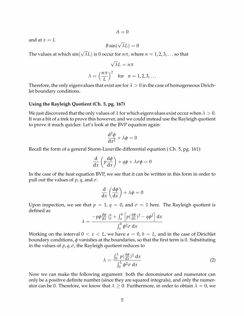
A = 0

and at x = LB sin(

√λL) = 0

The values at which sin(√

λL) is 0 occur for nπ, where n = 1, 2, 3, . . . so that√

λL = nπ

λ =(nπ

L

)2for n = 1, 2, 3, . . .

Therefore, the only eigenvalues that exist are for λ > 0 in the case of homogeneous Dirich-let boundary conditions.

Using the Rayleigh Quotient (Ch. 5, pg. 167)

We just discovered that the only values of λ for which eigenvalues exist occur when λ > 0.It was a bit of a trek to prove this however, and we could instead use the Rayleigh quotientto prove it much quicker. Let’s look at the BVP equation again:

d2φ

dx2 + λφ = 0

Recall the form of a general Sturm-Liouville differential equation ( Ch. 5, pg. 161):

ddx

(p

dφ

dx

)+ qφ + λσφ = 0

In the case of the heat equation BVP, we see that it can be written in this form in order topull out the values of p, q, and σ.

ddx

(dφ

dx

)+ λφ = 0

Upon inspection, we see that p = 1, q = 0, and σ = 1 here. The Rayleigh quotient isdefined as

λ =−pφ

dφdx |

ba +

∫ ba

[p(dφ

dx )2 − qφ2]

dx∫ ba φ2σ dx

Working on the interval 0 < x < L, we have a = 0, b = L, and in the case of Dirichletboundary conditions, φ vanishes at the boundaries, so that the first term is 0. Substitutingin the values of p, q, σ, the Rayleigh quotient reduces to

λ =

∫ L0 p(dφ

dx )2 dx∫ L0 φ2σ dx

(2)

Now we can make the following argument: both the denominator and numerator canonly be a positive definite number (since they are squared integrals), and only the numer-ator can be 0. Therefore, we know that λ ≥ 0. Furthermore, in order to obtain λ = 0, we

5

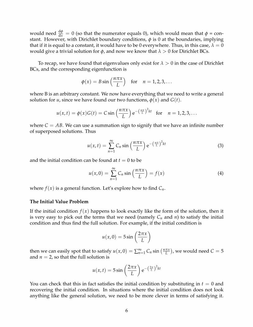
would need dφdx = 0 (so that the numerator equals 0), which would mean that φ = con-

stant. However, with Dirichlet boundary conditions, φ is 0 at the boundaries, implyingthat if it is equal to a constant, it would have to be 0 everywhere. Thus, in this case, λ = 0would give a trivial solution for φ, and now we know that λ > 0 for Dirichlet BCs.

To recap, we have found that eigenvalues only exist for λ > 0 in the case of DirichletBCs, and the corresponding eigenfunction is

φ(x) = B sin(nπx

L

)for n = 1, 2, 3, . . .

where B is an arbitrary constant. We now have everything that we need to write a generalsolution for u, since we have found our two functions, φ(x) and G(t).

u(x, t) = φ(x)G(t) = C sin(nπx

L

)e−( nπ

L )2kt for n = 1, 2, 3, . . .

where C = AB. We can use a summation sign to signify that we have an infinite numberof superposed solutions. Thus

u(x, t) =∞

∑n=1

Cn sin(nπx

L

)e−( nπ

L )2kt (3)

and the initial condition can be found at t = 0 to be

u(x, 0) =∞

∑n=1

Cn sin(nπx

L

)= f (x) (4)

where f (x) is a general function. Let’s explore how to find Cn.

The Initial Value Problem

If the initial condition f (x) happens to look exactly like the form of the solution, then itis very easy to pick out the terms that we need (namely Cn and n) to satisfy the initialcondition and thus find the full solution. For example, if the initial condition is

u(x, 0) = 5 sin(

2πxL

)then we can easily spot that to satisfy u(x, 0) = ∑∞

n=1 Cn sin(nπx

L), we would need C = 5

and n = 2, so that the full solution is

u(x, t) = 5 sin(

2πxL

)e−( 2π

L )2kt

You can check that this in fact satisfies the initial condition by substituting in t = 0 andrecovering the initial condition. In situations where the initial condition does not lookanything like the general solution, we need to be more clever in terms of satisfying it.

6

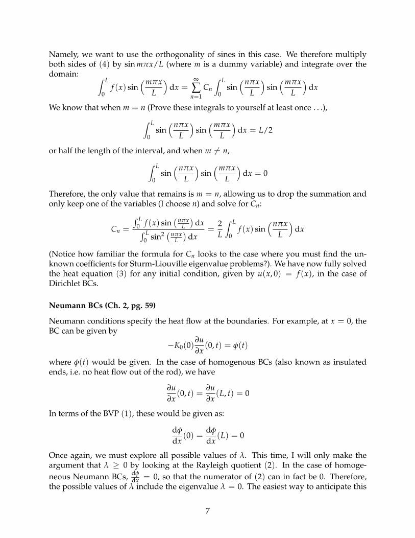
Namely, we want to use the orthogonality of sines in this case. We therefore multiplyboth sides of (4) by sin mπx/L (where m is a dummy variable) and integrate over thedomain: ∫ L

0f (x) sin

(mπxL

)dx =

∞

∑n=1

Cn

∫ L

0sin(nπx

L

)sin(mπx

L

)dx

We know that when m = n (Prove these integrals to yourself at least once . . .),∫ L

0sin(nπx

L

)sin(mπx

L

)dx = L/2

or half the length of the interval, and when m 6= n,∫ L

0sin(nπx

L

)sin(mπx

L

)dx = 0

Therefore, the only value that remains is m = n, allowing us to drop the summation andonly keep one of the variables (I choose n) and solve for Cn:

Cn =

∫ L0 f (x) sin

(nπxL)

dx∫ L0 sin2 (nπx

L)

dx=

2L

∫ L

0f (x) sin

(nπxL

)dx

(Notice how familiar the formula for Cn looks to the case where you must find the un-known coefficients for Sturm-Liouville eigenvalue problems?). We have now fully solvedthe heat equation (3) for any initial condition, given by u(x, 0) = f (x), in the case ofDirichlet BCs.

Neumann BCs (Ch. 2, pg. 59)

Neumann conditions specify the heat flow at the boundaries. For example, at x = 0, theBC can be given by

−K0(0)∂u∂x

(0, t) = φ(t)

where φ(t) would be given. In the case of homogenous BCs (also known as insulatedends, i.e. no heat flow out of the rod), we have

∂u∂x

(0, t) =∂u∂x

(L, t) = 0

In terms of the BVP (1), these would be given as:

dφ

dx(0) =

dφ

dx(L) = 0

Once again, we must explore all possible values of λ. This time, I will only make theargument that λ ≥ 0 by looking at the Rayleigh quotient (2). In the case of homoge-neous Neumann BCs, dφ

dx = 0, so that the numerator of (2) can in fact be 0. Therefore,the possible values of λ include the eigenvalue λ = 0. The easiest way to anticipate this

7

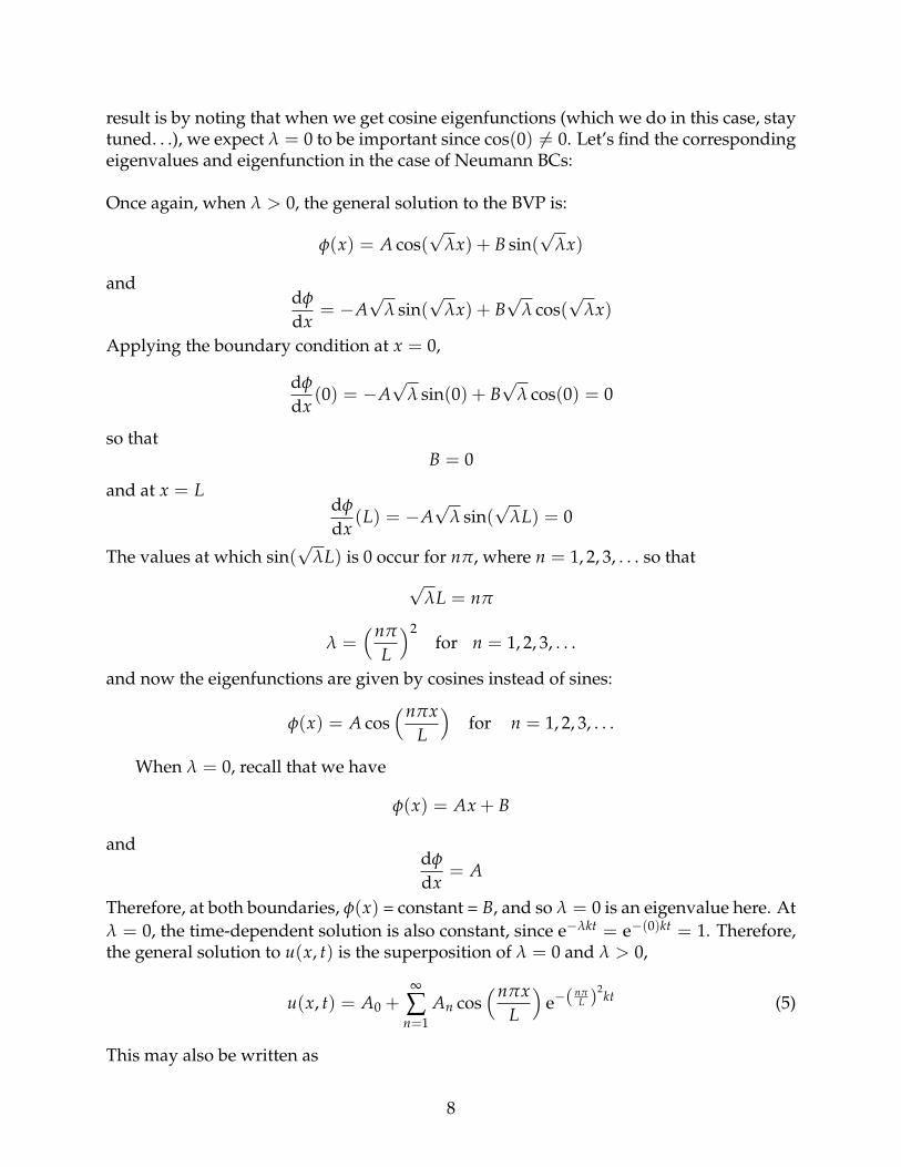
result is by noting that when we get cosine eigenfunctions (which we do in this case, staytuned. . .), we expect λ = 0 to be important since cos(0) 6= 0. Let’s find the correspondingeigenvalues and eigenfunction in the case of Neumann BCs:

Once again, when λ > 0, the general solution to the BVP is:

φ(x) = A cos(√

λx) + B sin(√

λx)

anddφ

dx= −A

√λ sin(

√λx) + B

√λ cos(

√λx)

Applying the boundary condition at x = 0,

dφ

dx(0) = −A

√λ sin(0) + B

√λ cos(0) = 0

so thatB = 0

and at x = Ldφ

dx(L) = −A

√λ sin(

√λL) = 0

The values at which sin(√

λL) is 0 occur for nπ, where n = 1, 2, 3, . . . so that√

λL = nπ

λ =(nπ

L

)2for n = 1, 2, 3, . . .

and now the eigenfunctions are given by cosines instead of sines:

φ(x) = A cos(nπx

L

)for n = 1, 2, 3, . . .

When λ = 0, recall that we have

φ(x) = Ax + B

anddφ

dx= A

Therefore, at both boundaries, φ(x) = constant = B, and so λ = 0 is an eigenvalue here. Atλ = 0, the time-dependent solution is also constant, since e−λkt = e−(0)kt = 1. Therefore,the general solution to u(x, t) is the superposition of λ = 0 and λ > 0,

u(x, t) = A0 +∞

∑n=1

An cos(nπx

L

)e−( nπ

L )2kt (5)

This may also be written as

8

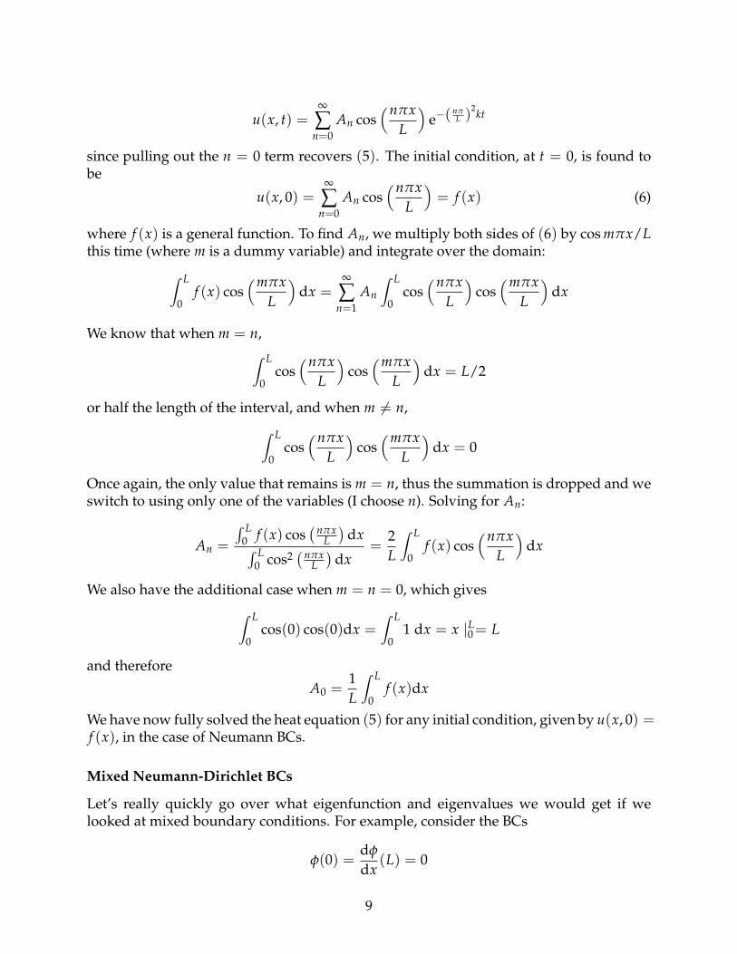
u(x, t) =∞

∑n=0

An cos(nπx

L

)e−( nπ

L )2kt

since pulling out the n = 0 term recovers (5). The initial condition, at t = 0, is found tobe

u(x, 0) =∞

∑n=0

An cos(nπx

L

)= f (x) (6)

where f (x) is a general function. To find An, we multiply both sides of (6) by cos mπx/Lthis time (where m is a dummy variable) and integrate over the domain:∫ L

0f (x) cos

(mπxL

)dx =

∞

∑n=1

An

∫ L

0cos

(nπxL

)cos

(mπxL

)dx

We know that when m = n,∫ L

0cos

(nπxL

)cos

(mπxL

)dx = L/2

or half the length of the interval, and when m 6= n,∫ L

0cos

(nπxL

)cos

(mπxL

)dx = 0

Once again, the only value that remains is m = n, thus the summation is dropped and weswitch to using only one of the variables (I choose n). Solving for An:

An =

∫ L0 f (x) cos

(nπxL)

dx∫ L0 cos2

(nπxL)

dx=

2L

∫ L

0f (x) cos

(nπxL

)dx

We also have the additional case when m = n = 0, which gives∫ L

0cos(0) cos(0)dx =

∫ L

01 dx = x |L0 = L

and therefore

A0 =1L

∫ L

0f (x)dx

We have now fully solved the heat equation (5) for any initial condition, given by u(x, 0) =f (x), in the case of Neumann BCs.

Mixed Neumann-Dirichlet BCs

Let’s really quickly go over what eigenfunction and eigenvalues we would get if welooked at mixed boundary conditions. For example, consider the BCs

φ(0) =dφ

dx(L) = 0

9

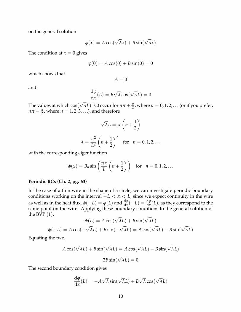
on the general solution

φ(x) = A cos(√

λx) + B sin(√

λx)

The condition at x = 0 gives

φ(0) = A cos(0) + B sin(0) = 0

which shows thatA = 0

anddφ

dx(L) = B

√λ cos(

√λL) = 0

The values at which cos(√

λL) is 0 occur for nπ + π2 , where n = 0, 1, 2, . . . (or if you prefer,

nπ − π2 , where n = 1, 2, 3, . . .), and therefore

√λL = π

(n +

12

)

λ =π2

L2

(n +

12

)2

for n = 0, 1, 2, . . .

with the corresponding eigenfunction

φ(x) = Bn sin(

πxL

(n +

12

))for n = 0, 1, 2, . . .

Periodic BCs (Ch. 2, pg. 63)

In the case of a thin wire in the shape of a circle, we can investigate periodic boundaryconditions working on the interval −L < x < L, since we expect continuity in the wireas well as in the heat flux, φ(−L) = φ(L) and dφ

dx (−L) = dφdx (L), as they correspond to the

same point on the wire. Applying these boundary conditions to the general solution ofthe BVP (1):

φ(L) = A cos(√

λL) + B sin(√

λL)

φ(−L) = A cos(−√

λL) + B sin(−√

λL) = A cos(√

λL)− B sin(√

λL)

Equating the two,

A cos(√

λL) + B sin(√

λL) = A cos(√

λL)− B sin(√

λL)

2B sin(√

λL) = 0

The second boundary condition gives

dφ

dx(L) = −A

√λ sin(

√λL) + B

√λ cos(

√λL)

10

dφ

dx(−L) = −A

√λ sin(−

√λL) + B

√λ cos(−

√λL) = A

√λ sin(

√λL) + B

√λ cos(

√λL)

Once again, equating the two,

−A√

λ sin(√

λL) + B√

λ cos(√

λL) = A√

λ sin(√

λL) + B√

λ cos(√

λL)

2A√

λ sin(√

λL) = 0

Therefore, both boundary conditions show the same result, namely that in order to geteigenvalues for λ > 0, we need

sin(√

λL) = 0

giving eigenvalues

λ =(nπ

L

)2for n = 1, 2, 3, . . .

with a corresponding eigenfunction,

φ(x) = an cos(nπx

L

)+ bn sin

(nπxL

)for n = 1, 2, 3, . . .

Prove to yourself that you also get an eigenvalue for λ = 0, since there is a cosine eigen-function term. Thus the general solution u(x, t)is given by

u(x, t) = a0 +∞

∑n=1

an cos(nπx

L

)e−( nπ

L )2kt +

∞

∑n=1

bn sin(nπx

L

)e−( nπ

L )2kt

and the initial condition is

u(x, 0) = f (x) =∞

∑n=0

an cos(nπx

L

)+

∞

∑n=1

bn sin(nπx

L

)after absorbing the n = 0 term into an. In order to find the unknown coefficients, we canfirst multiply both sides by sin(mπx/L) and integrate over the domain −L < x < L∫ L

−Lf (x) sin

(mπxL

)dx =

∞

∑n=0

an

∫ L

−Lcos

(nπxL

)sin(mπx

L

)dx +

∞

∑n=1

bn

∫ L

−Lsin(nπx

L

)sin(mπx

L

)dx

We know that when m = n,∫ L

−Lsin(nπx

L

)sin(mπx

L

)dx = L

or half the length of the interval, and 0 otherwise. Also,∫ L

−Lcos

(nπxL

)sin(mπx

L

)dx = 0

Since sine is an odd function and cosine is an even function, their product is an odd func-tion. The integral of an odd function over a symmetric interval is 0. Therefore, the only

11

value that remains is m = n, for the second term, and thus we can pick out the bn terms.We can likewise do the same in order to find the an terms, specifically by multiplying bothsides by cos(mπx/L) and integrating over the domain. Thus we find that

a0 =1

2L

∫ L

−Lf (x)dx

an =1L

∫ L

−Lf (x) cos

(nπxL

)dx

bn =1L

∫ L

−Lf (x) sin

(nπxL

)dx

The Wave Equation (Ch. 4, pg. 142)

The wave equation is given by∂2u∂t2 = c2 ∂2u

∂x2 (7)

This is second-order in time and second-order in space, therefore we expect 2 initial con-ditions and 2 boundary conditions in order to find the full solution. We will investigatethe wave equation with fixed ends, so that

u(0, t) = u(L, t) = 0

and initial conditionsu(x, 0) = f (x),

∂u∂t

(x, 0) = g(x)

Applying MSV, and assuming the solution u(x, t) = φ(x)G(t),

φ(x)d2Gdt2 = c2G(t)

d2φ

dx2

and dividing by φ(x)G(t)c2, we obtain 2 ODEs

1c2G

d2Gdt2 =

1φ

d2φ

dx2

with the homogeneous boundary conditions

φ(0) = φ(L) = 0

The motivation behind choosing a sign for the separation constant λ comes from look-ing at the boundary conditions; we want φ to be 0 at both ends, suggesting that it mustoscillate in order to satisfy these conditions. Therefore, we choose −λ,

1c2G

d2Gdt2 =

1φ

d2φ

dx2 = −λ

12

This gives the boundary value problem with the same Dirichlet boundary conditions thatwe saw for the heat equation, so I will go ahead and write down the eigenvalues andcorresponding eigenfunction, noting that we found eigenvalues only when λ > 0 withthese boundary conditions:

λ =(nπ

L

)2for n = 1, 2, 3, . . .

φ(x) = B sin(nπx

L

)for n = 1, 2, 3, . . .

Now looking at the time-dependent equation, we have

d2Gdt2 + c2λG = 0

Notice that this is a second-order, constant coefficient ODE with a general solution of theform

G(t) = c1 cos(c√

λt) + c2 sin(c√

λt)

and substituting in the eigenvalue that we found previously,

G(t) = c1 cos(

nπctL

)+ c2 sin

(nπct

L

)Therefore, the general solution may be found by taking the product of φ(x) and G(t) andsumming over all possible integer values of n,

u(x, t) =∞

∑n=1

[An sin

(nπxL

)cos

(nπct

L

)+ Bn sin

(nπxL

)sin(

nπctL

)]The initial conditions are satisfied by

u(x, 0) = f (x) =∞

∑n=1

An sin(nπx

L

)and

∂u∂t

(x, 0) = g(x) =∞

∑n=1

Bnnπc

Lsin(nπx

L

)In order to find the An terms, we multiply both sides by sin

(mπxL)

and integrate over thedomain, once again taking advantage of the orthogonality of sines. We therefore find that

An =2L

∫ L

0f (x) sin

(nπxL

)dx

The same technique is used to find Bn, which is then defined by

Bnnπc

L=

2L

∫ L

0g(x) sin

(nπxL

)dx

and therefore,

Bn =2

nπc

∫ L

0g(x) sin

(nπxL

)dx

13

Laplace’s Equation Inside a Rectangle (Ch. 2, pg. 71)

Laplace’s equation in cartesian coordinates is given by

∂2u∂x2 +

∂2u∂y2 = 0

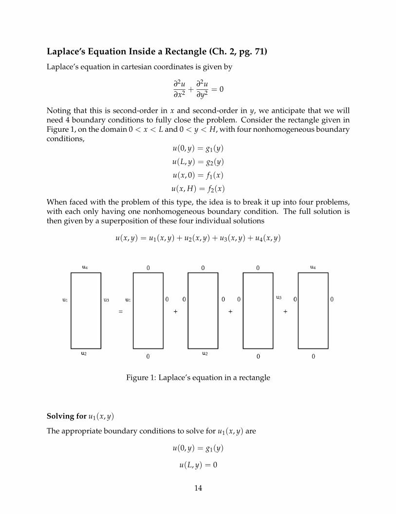
Noting that this is second-order in x and second-order in y, we anticipate that we willneed 4 boundary conditions to fully close the problem. Consider the rectangle given inFigure 1, on the domain 0 < x < L and 0 < y < H, with four nonhomogeneous boundaryconditions,

u(0, y) = g1(y)

u(L, y) = g2(y)

u(x, 0) = f1(x)

u(x, H) = f2(x)

When faced with the problem of this type, the idea is to break it up into four problems,with each only having one nonhomogeneous boundary condition. The full solution isthen given by a superposition of these four individual solutions

u(x, y) = u1(x, y) + u2(x, y) + u3(x, y) + u4(x, y)

Figure 1: Laplace’s equation in a rectangle

Solving for u1(x, y)

The appropriate boundary conditions to solve for u1(x, y) are

u(0, y) = g1(y)

u(L, y) = 0

14

u(x, 0) = 0

u(x, H) = 0

Let’s assume that we can write the solution for u as a product of two functions, u1(x, y) =h(x)φ(y) so that Laplace’s equation can be re-written as

φ(y)d2hdx2 + h(x)

d2φ

dy2 = 0

Dividing through by φ(y)h(x) and bringing the equation for φ to the right-hand side, wehave

1h

d2hdx2 = − 1

φ

d2φ

dy2

Before deciding what sign of λ to choose, let’s think about the boundary conditions forthis particular problem:

u(0, y) = h(0)φ(y) = g1(y)

u(L, y) = h(L)φ(y) = 0

u(x, 0) = h(x)φ(0) = 0

u(x, H) = h(x)φ(H) = 0

The boundary conditions imply that

u(0, y) = g1(y)

h(L) = 0

φ(0) = 0

φ(H) = 0

Note that we have two homogeneous boundary conditions for φ(y), and we thereforeexpect φ to oscillate in order to satisfy these conditions. This means that we should setthe separation constant to λ, so that the equations look like

1h

d2hdx2 = − 1

φ

d2φ

dy2 = λ

d2φ

dy2 + λφ = 0

andd2hdx2 − λh = 0

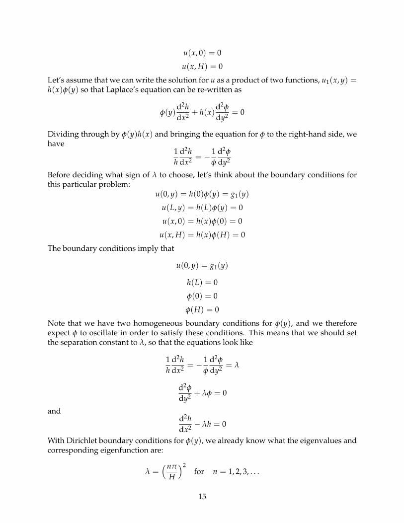
With Dirichlet boundary conditions for φ(y), we already know what the eigenvalues andcorresponding eigenfunction are:

λ =(nπ

H

)2for n = 1, 2, 3, . . .

15

φ(y) = sin(nπy

H

)for n = 1, 2, 3, . . .

Also, note that previously when we solved this boundary value problem for the heatequation, we proved that the only eigenvalues that existed in the case of Dirichlet bound-ary conditions were when λ > 0. The equation for h(x) has the general solution

h(x) = A sinh(√

λx) + B cosh(√

λx)

and we have one homogeneous boundary condition at our disposal, h(L) = 0. Becausethis boundary condition is given at x = L, it is to our benefit that we shift the origin tox = L in order to get one of the terms in the general solution to disappear after applyingthe homogeneous boundary condition. Therefore,

h(x) = A sinh√

λ(x− L) + B cosh√

λ(x− L)

so thath(L) = A sinh(0) + B cosh(0) = 0

and therefore B = 0. This is allowed because the differential equation does not changeupon performing the shift, and is therefore invariant upon translation. The solution forh(x) is then

h(x) = A sinhnπ

H(x− L)

where the eigenvalue λ was found when we solved for φ. Now the full solution foru1(x, y) is

u1(x, y) =∞

∑n=1

An sin(nπy

H

)sinh

nπ

H(x− L)

and the last nonhomogenous boundary condition, u(0, y) = g1(y) allows us to solve forthe unknown coefficients An.

u1(0, y) = g1(y) =∞

∑n=1

An sin(nπy

H

)sinh

nπ

H(−L)

Once again, multiply both sides by sin(mπy/H) and integrate over the domain so that

An =2

H sinh nπH (−L)

∫ H

0g1(y) sin

(nπyH

)dy

There are a few things worth mentioning here. The first is to notice that the hyperbolicterm is completely constant in this integral, and that is why we are able to pull it out ofthe integral and bring it over to the other side. The second point is that the sine functionis in terms of y, which is the reason that we are integrating in y from 0 to H, (which is thedomain of y here). This is also the reason why we obtain a 2/H instead of the usual 2/Lterm in front of the integral to evalue An. We now have the full solution for u1(x, y).

16

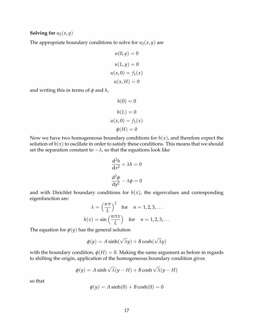
Solving for u2(x, y)

The appropriate boundary conditions to solve for u2(x, y) are

u(0, y) = 0

u(L, y) = 0

u(x, 0) = f1(x)

u(x, H) = 0

and writing this in terms of φ and h,

h(0) = 0

h(L) = 0

u(x, 0) = f1(x)

φ(H) = 0

Now we have two homogeneous boundary conditions for h(x), and therefore expect thesolution of h(x) to oscillate in order to satisfy these conditions. This means that we shouldset the separation constant to −λ, so that the equations look like

d2hdx2 + λh = 0

d2φ

dy2 − λφ = 0

and with Dirichlet boundary conditions for h(x), the eigenvalues and correspondingeigenfunction are:

λ =(nπ

L

)2for n = 1, 2, 3, . . .

h(x) = sin(nπx

L

)for n = 1, 2, 3, . . .

The equation for φ(y) has the general solution

φ(y) = A sinh(√

λy) + B cosh(√

λy)

with the boundary condition, φ(H) = 0. Making the same argument as before in regardsto shifting the origin, application of the homogeneous boundary condition gives

φ(y) = A sinh√

λ(y− H) + B cosh√

λ(y− H)

so thatφ(y) = A sinh(0) + B cosh(0) = 0

17

and therefore B = 0. The solution for φ(y) is then

φ(y) = A sinhnπ

L(y− H)

where the eigenvalue λ was found when solving for h(x). The full solution for u2(x, y) is

u2(x, y) =∞

∑n=1

Bn sin(nπx

L

)sinh

nπ

L(y− H)

and the last nonhomogenous boundary condition, u(x, 0) = f1(x) allows us to solve forthe unknown coefficients Bn.

u2(x, 0) = f1(x) =∞

∑n=1

Bn sin(nπx

L

)sinh

nπ

L(−H)

Multiply both sides by sin(mπx/L) and integrate over the domain in x so that we are leftwith

Bn =2

L sinh nπL (−H)

∫ L

0f1(x) sin

(nπxL

)dx

I will leave it up to you to find u3(x, y) and u4(x, y) Note that with these solutions, youdo not have to shift the origin, because the one homogeneous boundary condition will begiven at 0.

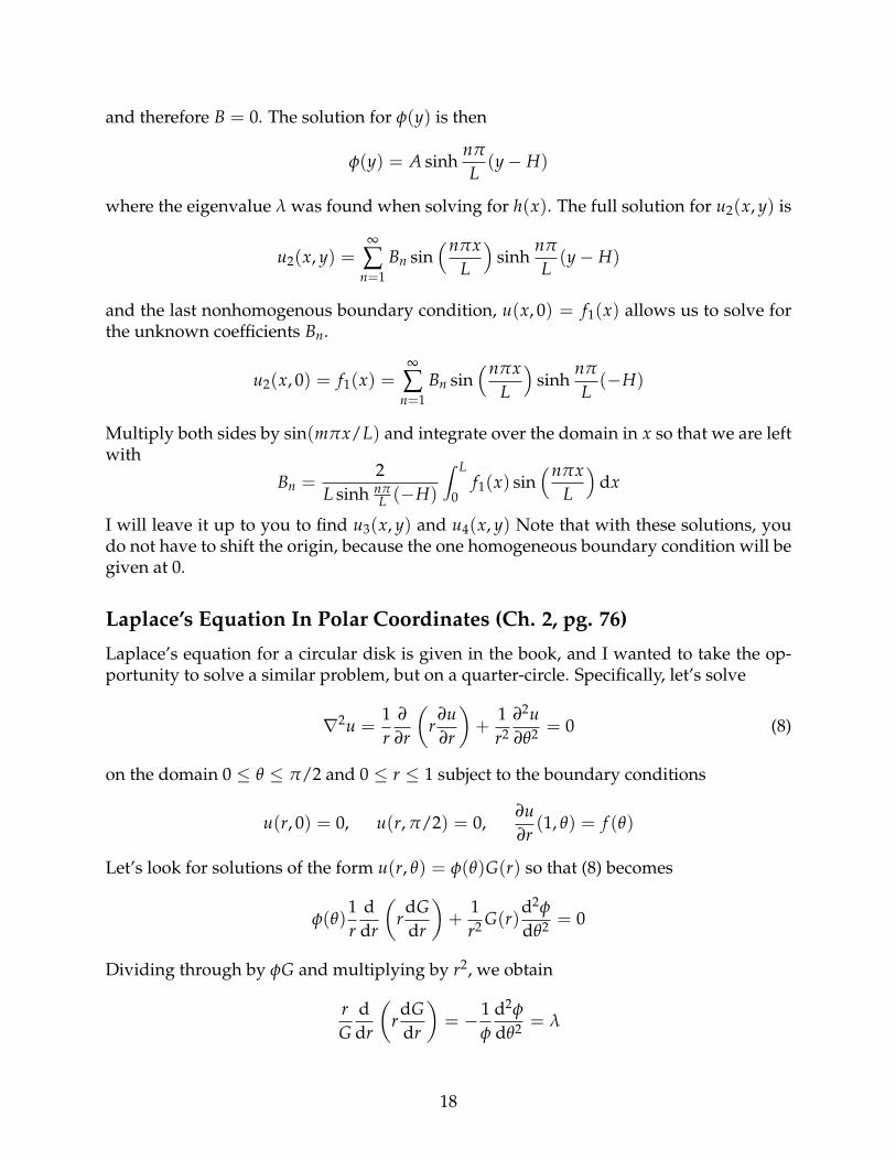
Laplace’s Equation In Polar Coordinates (Ch. 2, pg. 76)

Laplace’s equation for a circular disk is given in the book, and I wanted to take the op-portunity to solve a similar problem, but on a quarter-circle. Specifically, let’s solve

∇2u =1r

∂

∂r

(r

∂u∂r

)+

1r2

∂2u∂θ2 = 0 (8)

on the domain 0 ≤ θ ≤ π/2 and 0 ≤ r ≤ 1 subject to the boundary conditions

u(r, 0) = 0, u(r, π/2) = 0,∂u∂r

(1, θ) = f (θ)

Let’s look for solutions of the form u(r, θ) = φ(θ)G(r) so that (8) becomes

φ(θ)1r

ddr

(r

dGdr

)+

1r2 G(r)

d2φ

dθ2 = 0

Dividing through by φG and multiplying by r2, we obtain

rG

ddr

(r

dGdr

)= − 1

φ

d2φ

dθ2 = λ

18

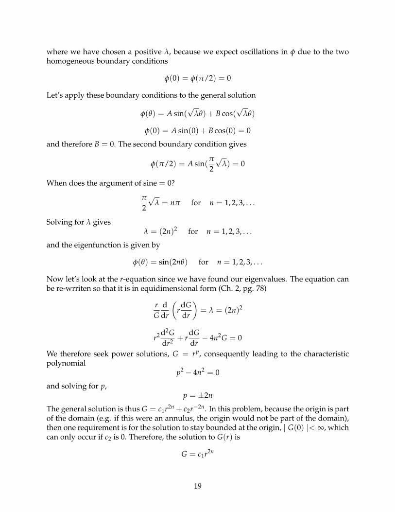
where we have chosen a positive λ, because we expect oscillations in φ due to the twohomogeneous boundary conditions

φ(0) = φ(π/2) = 0

Let’s apply these boundary conditions to the general solution

φ(θ) = A sin(√

λθ) + B cos(√

λθ)

φ(0) = A sin(0) + B cos(0) = 0

and therefore B = 0. The second boundary condition gives

φ(π/2) = A sin(π

2

√λ) = 0

When does the argument of sine = 0?

π

2

√λ = nπ for n = 1, 2, 3, . . .

Solving for λ givesλ = (2n)2 for n = 1, 2, 3, . . .

and the eigenfunction is given by

φ(θ) = sin(2nθ) for n = 1, 2, 3, . . .

Now let’s look at the r-equation since we have found our eigenvalues. The equation canbe re-wrriten so that it is in equidimensional form (Ch. 2, pg. 78)

rG

ddr

(r

dGdr

)= λ = (2n)2

r2 d2Gdr2 + r

dGdr− 4n2G = 0

We therefore seek power solutions, G = rp, consequently leading to the characteristicpolynomial

p2 − 4n2 = 0

and solving for p,p = ±2n

The general solution is thus G = c1r2n + c2r−2n. In this problem, because the origin is partof the domain (e.g. if this were an annulus, the origin would not be part of the domain),then one requirement is for the solution to stay bounded at the origin, | G(0) |< ∞, whichcan only occur if c2 is 0. Therefore, the solution to G(r) is

G = c1r2n

19

and the general solution to u(r, θ) is given by

u(r, θ) =∞

∑n=1

Anr2n sin(2nθ)

There is still one nonhomogeneous boundary condition to apply, ∂u∂r (1, θ). Therefore,

∂u∂r

(1, θ) = f (θ) =∞

∑n=1

2nAn12n−1 sin(2nθ)

In order to find An, multiply both sides by sin(2mθ) and integrate from 0 to π/2. Weexpect the sine orthogonality integral to return half of the interval (please prove this toyourself), and therefore ∫ π/2

0sin2(2nθ)dθ = π/4

so that

An =2

nπ

∫ π/2

0f (θ) sin(2nθ)dθ

Another interesting problem to consider is solving the Laplace equation in polar coordi-nates outside of a circular disk. Let’s quickly explore that with the boundary conditionu(a, θ) = f (θ). Please find on pgs. 78-79 how to obtain eigenvalues and the correspond-ing eigenfunction in the case of periodic boundary conditions,

φ(θ) = cos(nθ) + sin(nθ) for n = 0, 1, 2, . . .

The full equation for G(r) after also taking into consideration the λ = 0 eigenvalue is

G(r) = c1rn + d1r−n + c0 + d0 ln(r)

If we are trying to solve Laplace’s equation outside of the circle, we would not expectto worry about solutions blowing up at the origin, since that is not our area of interest.Instead, we would expect u → 0 as r → ∞ and therefore c1 and d0 must be 0, otherwisethe solution would not decay at ∞. Therefore,

G = c0 + d1r−n

so that the general solution takes the form

u(r, θ) =∞

∑n=0

Anr−n cos(nθ) +∞

∑n=1

Bnr−n sin(nθ)

where the c0 is recovered by substituting n = 0 into the general solution, and has thusbeen absorbed in the cosine summation. The book can be consulted to evaluate An andBn.

20

Sturm-Liouville Eigenvalue Problems (Ch.5, pg. 161)

The regular Sturm-Liouville differential equation is given by

ddx

(p(x)

dφ

dx

)+ q(x)φ + λσ(x)φ = 0

on the interval a < x < b. Some things to note:

• Any second-order, linear ODE may be written in this form by use of an integratingfactor

• All eigenvalues λ are real, and there are an infinite number of eigenvalues

• Corresponding to each eigenvalue λn, there is an eigenfunction φn(x) that has n− 1zeros on the interval a < x < b

• Eigenfunctions are orthogonal relative to the weight function σ(x), and the orthog-onality relation is given by∫ b

aφn(x)φm(x)σ(x)dx = 0 when n 6= m

• Any piecewise smooth function f (x) can be represented by a generalized Fourierseries of the eigenfunctions:

f (x) ∼∞

∑n=1

anφn(x)

If we would like to solve for an, we can do as before and multiply both sides by theeigenfunction (using the dummy variable, m) and integrate over the domain. Fromthe previous theorem, we know that the eigenfunctions are orthogonal, thereforeonly the n = m term will survive and

an =

∫ ba f (x)φn(x)σ(x)dx∫ b

a φ2n(x)σ(x)dx

Let’s look at the most general second-order ODE that we can come up with,

d2φ

dx2 + α(x)dφ

dx+ [λβ(x) + γ(x)]φ = 0

Multiply this by some function H(x)

Hd2φ

dx2 + α(x)Hdφ

dx+ [λβ(x) + γ(x)]φH = 0

21

and now let α(x)H= dH/dx in order to create a perfect derivative in the first term,

Hd2φ

dx2 +dHdx

+ [λβ(x) + γ(x)]φH = 0

This allows the equation to be written in SL form,

ddx

(H

dφ

dx

)+ [λβ(x) + γ(x)]φH = 0

The only thing left to find is what H(x) is; don’t forget that we let α(x)H= dH/dx . Wecan readily integrate this equation to give the integrating factor,

dHdx

= α(x)H

dHH

= α(x) dx

ln(H) =∫ x

α(x′)dx′

H = e∫ x

α(x′)dx′

Thus we can find H(x) if α(x) is known, and thus we have successfully re-written thesecond-order general ODE into SL form, where

p(x) = H, q(x) = γ(x)H, σ(x) = β(x)H

Green’s function (Ch. 9, pg. 393)

The Green’s function is another tool for solving nonhomogeneous problems subject totwo homogeneous boundary conditions. If we are given a nonhomogeneous problem

L(u) = f (x)

where L is a linear operator acting on u, the solution may be found by seeking the Green’sfunction, since

u(x) =∫ b

af (x0)G(x, x0)dx0

The Green’s function G(x, x0), is the response at x due to a concentrated source at x0. Wewill do an example to illustrate how the Green’s function works.

22

Green’s function Example

Let’s solve the ODE

y′′ + 3y′ + 2y = 0 with y(0) = y′(0) = 0

using Green’s functions (the prime denotes derivatives in x). The first step is to applythe linear operator to the Green’s function G(x, x0) and set it equal to the delta function,noting that it must satisfy the same boundary conditions:

1.G′′ + 3G′ + 2G = δ(x− x0) with G(0, x0) = G′(0, x0) = 0

When x 6= x0, G′′ + 3G′ + 2G = 0.

2. Now solve this equation twice, once to the left of the source x0, and once to the right.This is a 2nd order constant coefficient ODE with the characteristic polynomial:

r2 + 3r + 2 = 0

(r + 2)(r + 1) = 0

r = −2,−1

so that

G(x, x0) ={

Ae−2x + Be−x x < x0Ce−2x + De−x x > x0

}3. Now we apply our boundary conditions to evalue 2/4 of the unknown coefficients.

The two boundary conditions will be applied to the interval x < x0 in this specialsituation, and we find that they imply that A = B = 0. Therefore,

G(x, x0) ={

0 x < x0Ce−2x + De−x x > x0

}4. There are still two more conditions to satisfy, namely continuity of G at x = x0, and

a jump in the n− 1 derivative at x = x0. The former gives

Ce−2x0 + De−x0 = 0

C = −Dex0

5. The jump condition comes from integrating the original equation and noting thatthe integral of the delta function is 1.

G′ |x+0

x−0= 1

where the other terms equated to 0 since they are continuous across x = x0. There-fore, we have

(−2Ce−2x0 − De−x0)− 0 = 1

23

and solving the two equations simultaneously, we find that

D = ex0

C = −e2x0

so that

G(x, x0) ={

0 x < x0−e2x0e−2x + ex0e−x x > x0

}6. Therefore, the solution is given by

y(x) =∫ x0

0(−e2(x0−x) + e(x0−x) f (x0)dx0

This example is a bit weird in the sense that on the left side of x0, there is no Green’s func-tion, but the symmetry to the right of x0 can still be seen and exploited in order to writethe solution. One thing to note is that for higher-order derivatives (e.g. for a derivativeof order n), the Green’s function will always have a jump in the n− 1 derivative, and willbe continuous in all lower derivatives.

Fourier Transforms (Ch. 10, pg. 445)

In order to illustrate how to use Fourier Transforms, I will do an example from the bookgiven on pg. 469. Let’s solve the diffusion equation with convection:

∂u∂t

= k∂2u∂x2 + c

∂u∂x

on the interval −∞ < x < ∞ with the initial condition u(x, 0) = f (x). Taking the Fouriertransform of this equation, we get

∂U∂t

= −ω2kU − icωU

which can be integrated∂U∂t

= U(−ω2k− icω)

∂UU

= (−ω2k− icω)∂t

U = A(ω)e(−ω2k−icω)t

In order to find the solution u(x, y), we need to find the inverse Fourier transform ofU(ω, t). This can be done by noting that

F−1[U] = F−1[A(ω)] ∗ F−1[e(−ω2k−icω)t]

24

where we can use the convolution theorem in order to find the inverse Fourier transformof the product of two functions. Prove to yourself that

F−1[A(ω)] = f (x)

which is the initial condition. Now for the second term,

F−1[e(−ω2k−icω)t] =∫ ∞

−∞e(−ω2k−icω)te−iωxdω

The important thing to note here is that this may be re-written as∫ ∞

−∞e(−ω2k−icω)te−iωxdω =

∫ ∞

−∞e−ω2kte−iω(x+ct)dω

In essence, we can introduce a new definition for x, such that x′ = x + ct. Therefore,

u(x + ct, t) =∫ ∞

−∞U(ω, t)e−iω(x+ct)dω =

∫ ∞

−∞U(ω, t)e−iωx′dω

We can now find the Fourier transform of above function, since we know from tables thatit will be a Gaussian. This gives us

∫ ∞

−∞e−ω2kte−iωx′dω =

√π

kte−x′2/4kt

√π

kte−(x+ct)2/4kt

All that is left to do is apply the convolution theorem, which states that

f ∗ g =1

2π

∫ ∞

−∞f (x)g(x− x)dx

In this case,f (x) = f (x)

or the initial condition, and

g(x) =√

π

kte−(x+ct)2/4kt

so thatu(x, t) = f ∗ g =

1√4πkt

∫ ∞

−∞f (x)e−(x+ct−x)2/4ktdx

25