Embed Size (px)
Citation preview

100
CHAPTER 5
IMAGE COMPRESSION TECHNIQUE USING
NONSUBSAMPLED CONTOURLET TRANSFORM
5.1 INTRODUCTION
Image compression is currently a well-known topic for
researchers. Due to fast growth of digital media and the following need for
reduced storage and to convey the image in an efficient way, better image
compression approach is required.
Among the rapid growth of digital technology in consumer
electronics, their requirement to protect raw image data for future editing
or repeated compression goes on increasing. Thus, image compression has
become a dynamic area of research in the field of image processing to
lessen file size. Wavelet and curvelet transformations are widely used
transformation techniques to carry out compression. But both have their
own limitations which affects overall performance of the compression
process. This research work focuses on presenting a non-linear image
compression technique that compresses image both radically and angularly.
Nonsubsampled Contourlet Transformation (NSCT) has the potential to
approximate the natural images comprising contours and oscillatory
patterns. In addition to this transformation, vector quantization technique is
used to remove the redundancies in the images. Finally, this technique uses
Hybrid Set Partitioning in Hierarchical Trees (HSPIHT) with Huffman for

101
efficient encoding process. The experimental results of Non-sub sampled
contourlet transformation, with vector quantization and HSPIHT are better
when compared with existing transformations techniques.
5.2 PROBLEMS IN WAVELET BASED CONTOURLET
TRANSFORM
A non-redundant transform is needed for image coding. Certain
types of non-redundant geometrical image transforms that depends on the
DFB have been presented by the researchers. The octave-band directional
filter banks which are introduced by Paul S Hong & Mark JT Smith (2002)
correspond to a new family of the DFB that attains radial decomposition as
well. The CRISP-contourlet is another transform proposed by Lu & Do
(2003), which is implemented based on the contourlet formation, other than
nonseparable filter banks are merely used. Truong & Oraintara (2005)
presented a Non-uniform DFB which is a modified form of CRISP-
contourlets and is the other non-redundant directional transform, which
also gives multiresolution.
Neither of the above non-redundant directional schemes have
been used in a practical image processing application. Ramin Eslami &
Hayder Radha (2008) introduced a Wavelet-Based Contourlet Transform
(WBCT), in which DFB is applied to all the feature subbands of wavelets
in an analogous way that one constructs contourlets. The major difference
is that, wavelets are used instead of the Laplacian pyramids in contourlets.
As a result, the WBCT is non-redundant and can be adapted for some
resourceful wavelet-based image coding methods.
The main drawbacks of the WBCT and other contourlet-based
transforms contain artifacts that are occurred by setting some transform

102
coefficients to zero for nonlinear approximation and also owing to
quantizing of the coefficients for coding.
The image focusing multiple objects contains more information
than those which just focus one object. This type of image is broadly used
in various areas such as remote sensing, medical imaging, computer vision
and robotics. Actually, all cameras used in computer visualization systems
are not pin-hole devices but consist of convex lenses. Therefore, they
endure from the problem of partial depth of field (Chunming Li et al 2004).
It is often not possible to get an image which contains all relevant objects
in focus. The objects in front of or behind the focus plane would be
blurred. To overcome this problem, image fusion is introduced by the
author in several images with different focal points are shared together to
create an image with all objects fully focused (Pan et al 1999). Over past
years, numbers of techniques were proposed by the researchers for
multifocus image fusion. The easiest multifocus image fusion technique in
spatial domain is to take the average of the source images pixel by pixel,
would lead to numerous unpredicted side effects like reduced difference
Yuancheng & Yang (2008). Various methods depends on multiscale
decomposition (MSD) as presented by Pajares & Cruz (2004).
Wavelet transform for 1-D piecewise smooth signals are better,
though it has severe limitations with high dimensional signals. 2D split
wavelet performs better at isolating the discontinuities at object edges, but
cannot effectively signify the line and the curve discontinuities. In contrast,
it can only capture restricted directional information. Accordingly, WT
based method cannot conserve the relevant features in source images well
and will possibly introduce some artifacts and variation in the combined
results (Yuancheng & Yang 2008). Minh N Do & Vetterli (2005) presented
a Contourlet Transform (CT) is a two dimensional image representation
103
method. It is attained by combining the directional filter bank (DFB) as
discussed by Burt & Adelson (1983); Bamberger & Smith (1992).
Compared with the traditional DWT, the CT is not only with multi-scale
and localization, but also with mulitdirection and anisotropy.
Consequently, the CT can symbolize edges and further singularities along
curves. On the other hand, CT possesses shift-invariance and results in
artifacts along the edges to some level. Arthur et al (2006) proposed a
transform known as nonsubsampled contourlet transform (NSCT).
The NSCT come into the perfect properties of the CT, and in the meantime
consist of shift invariance. In image fusion, the NSCT has more
information fusion together and is obtained and the influence of
misregistration on the fused information which can also be reduced. As a
result, the NSCT is more appropriate for image fusion and also in image
compression etc.
5.3 NONSUBSAMPLED CONTOURLET TRANSFORM:
FILTER DESIGN AND APPLICATIONS
Several image processing tasks are executed in a particular
domain other than the pixel domain, frequently using invertible linear
transformation. This linear transformation can be superfluous or not, based
on whether the set of basic functions is linear independent. By means of
redundancy, it is feasible to improve the set of fundamental functions so
that the representation is more resourceful in capturing several signal
behavior. Applications of imaging are of edge detection, contour detection,
denoising and image restoration that can significantly assistance from
redundant representations. In the situation of multiscale expansions
employed with filter banks, dropping the fundamental requirement
provides the chance of an expansion that is shift-invariant, a vital property
in a number of applications. For example in image denoising ,by means of

104
thresholding in the wavelet domain, the lack of shift-invariance reasons
pseudo-Gibbs phenomena in the region of singularities (Coifman &
Donoho 1995). Thus, most of the modern wavelet denoising routines
employ an expansion with low shift sensitivity than the standard maximally
decimated wavelet decomposition as explained in Chang et al (2000);
Sendur & Selesnick (2002) and Minh Do & Vetterli (2005) proposed a
contourlet transform which is a directional multiscale transform that is built
by combining the Laplacian pyramid (LP) and the directional filter bank
(DFB). Due to downsamplers and upsamplers present in both the LP and
DFB, the contourlet transform is not shift-invariant. The nonsubsampled
contourlet transform (NSCT) is obtained by coupling a nonsubsampled
pyramid structure with the nonsubsampled DFB.
Figure 5.1 Idealized frequency partitioning obtained with the NSCT
5.3.1 Nonsubsampled Contourlet Transform
The idea behind a fully shift invariant multiscale directional
expansion similar to contourlets is to obtain the frequency partitioning of

105
Figure 5.1 without resorting to critically sampled structures that have
periodically time-varying units such as downsamplers and upsamplers. The
NSCT construction can thus be divided into two parts: (1) A
nonsubsampled pyramid structure which ensures the multiscale property
and (2) A nonsubsampled DFB structure which gives directionality.
5.3.2 Nonsubsampled Pyramid
The shift sensitivity of the LP can be remedied by replacing it
with a 2-channel nonsubsampled 2-D filter bank structure. Such expansion
is similar to the 1-D a trous wavelet expansion Shensa (1993) and has a
redundancy of J + 1 when J is the number of decomposition stages.
The ideal frequency support of the low-pass filter at the j-th stage is the
region jjjj 2,
2x
2,
2. Accordingly, the support of the high-pass
filter is the complement of the low-pass support region on the
1j1j1j1j 2,
2x
2,
2square. The proposed structure is thus different
from the tensor product, a trous algorithm. It has j+1 redundancy.
By contrast, the 2-D a trous algorithm has 3j+1 redundancy.
5.3.3 Nonsubsampled Directional Filter Bank
The directional filter bank is constructed by combining critically
sampled fan filter banks and pre/post re-sampling operations. The result is
a tree-structured filter bank which splits the frequency plane into
directional wedges.
A fully shift-invariant directional expansion is obtained by
simply switching off the downsamplers and upsamplers in the DFB

106
equivalent filter bank. Due to multirate identities, this is equivalent to
switching off each of the downsamplers in the tree structure, while still
keeping the re-sampling operations that can be absorbed by the filters. This
results in a tree structure composed of two-channel nonsubsampled filter
banks. The NSCT is obtained by carefully combining the 2-D
nonsubsampled pyramid and the nonsubsampled DFB (NSDFB) Arthur et
al (2006).
The resulting filtering structure approximates the ideal partition
of the frequency plane displayed in Figure 5.2. It must be noted that,
different from the contourlet expansion, the NSCT has a redundancy given
by J0j j
l2R where jl2 is the number of directions at scale j.
Figure 5.2 Two kinds of desired responses (a) The pyramid desired
response (b) The fan desired response
The directional filter bank of Bamberger & Smith (1992) is
constructed by combining critically-sampled two-channel fan filter banks
and resampling operations. The result is a tree-structured filter bank that
splits the frequency plane in the directional wedges shown in Figure 5.3(a).

107
Figure 5.3 The directional filter bank (a) Ideal partitioning of the 2-
D frequency plane into 23 = 8 wedges (b) Equivalent
multi-channel filter bank structure. The number of
channels is L = 2l, where l is the number of stages in the
tree structure
Using multirate identities Bamberger & Smith (1992), the tree-
structured DFB can be put into the equivalent form shown in Figure 5.3
(b), where the downsampling/upsampling matrices Sk for 0 2l-1 are
given by Equation (5.1)
;12k2for;12k0for
)2,2(diag)2,2(diag
S 1l1l
1l
1l
1l
k (5.1)
with ‘l’ denoting the number of stages in the tree structure. It is
clear from the above that the DFB is not shift-invariant. A shift-invariant
directional expansion is obtained with a nonsubsampled DFB (NSDFB).
The NSDFB is constructed by eliminating the downsamplers and
upsamplers as in Figure 5.3(b). This is equivalent to switching off the
downsamplers in each two-channel filter bank in the DFB tree structure
and upsampling the filters accordingly. This results in a tree consisting of
two-channel nonsubsampled filter banks. The equivalent filter in the kth

108
channel of the analysis NSDFB tree is the filter )z(Ueqk as in Figure 5.3 (b).
Thus, each filter )z(Ueqk is a product of l simpler filters. Just like the DFB,
all NSFB’s in the NSDFB tree structure are obtained from a single NSFB
with fan filters (Figure 5.4b) which illustrates a four channel
decomposition. Note that in the second level, the upsampled fan filters
1,0i),z(U Qi have checker-board frequency support, and when combined
with the filters in the first level, gives the four directional frequency
decomposition that is shown in Figure 5.4. The synthesis filter bank is
obtained similarly. Just like the NSP case, each filter bank in the NSDFB
tree has the same computational complexity as that of the prototype NSFB.
Figure 5.4 A four-channel nonsubsampled directional filter bank
constructed with two-channel fan filter banks
(a) Filtering structure (b) Corresponding frequency
decomposition
Figure 5.4(a) shows a four-channel filtering structure the
equivalent filter in each channel is given by )z(U)z(U)z(U Qji
eqk .
Figure 5.4(b) shows the corresponding frequency decomposition.

109
5.4 APPLICATIONS OF NON-SUBSAMPLED
CONTOURLET TRANSFORM
5.4.1 Image Denoising
In order to illustrate the potential of the NSCT designed using
the techniques previously discussed an Additive White Gaussian Noise
(AWGN) removal is implemented from the images by means of
thresholding estimators, and tested the NSCT fewer than two denoising
schemes described below:
1) Hard Threshold
For the hard threshold estimator, a global threshold
ijnj,i KT for each directional subband is chosen. This has been termed K-
sigma thresholding (Starck et al 2002). Set K = 4 for the finer scale and
K = 3 for the remaining ones. This method known as NSWT-HT when
applied to NSWT coefficients and NSCT-HT when applied to NSCT
coefficients. Five scales of decomposition are used for both NSCT and
NSWT. For the NSCT 4, 8, 8, 16, 16 directions in the scales are used from
coarser to finer respectively.
2) Local Adaptive Shrinkage
Perform soft thresholding (shrinkage) independently in each
subband. The threshold (Grace Chang et al 2000) is chosen by
Equation (5.2).
n,j,i
ijN2
j,iT (5.2)

110
where n,j,i denotes the variance of the n-th coefficient at the ith
directional subband of the jth scale, and ijN2 is the noise variance at scale j
and direction i. It is shown in Grace Chang et al et al (2000) that shrinkage
estimation with x
2T , and assuming X generalized Gaussian distributed,
yields a risk within 5% of the optimal Bayes risk. Po & Do (2006) studied
that contourlet coefficients are well modelled by generalized Gaussian
distributions. The signal variances are estimated locally using the
neighbouring coefficients contained in a square window within each
subband and a maximum likelihood estimator. The noise variance in each
subband is inferred using a Monte-Carlo technique where the variances are
computed for a few normalized noise images and then averaged to stabilize
the results. This method is known as local adaptive shrinkage (LAS).
Effectively, LAS method is a simplified version of the denoising method
proposed in Grace Chang et al (2000) that works in the NSCT or NSWT
domain.
The other applications of NSCT is image enhancement, image
fusion, image compression, applications of medical image analysis, video
compression etc.
5.4.2 Advantages of NSCT
The nonsubsampled contourlet transform (NSCT) not only has
multiresolution but has multidirectional properties
By using non-subsampled contourlet transform ,coefficients in
small-scale and gradient information of each colour channel is
identified efficiently

111
The NSCT is a fully shift-invariant, multi scale, and multi
direction expansion that have a fast implementation. Here,
filters are designed with better frequency selectivity, thereby
achieving better sub band decomposition
5.5 PROPOSED METHOD USING NON-SUBSAMPLED
CONTOURLET TRANSFORM
The basic steps of the proposed image compression algorithm
are shown in Figure 5.5. All these steps are invertible, therefore lossless,
except for the Quantize step. Quantizing is the process of reduction of the
precision of the floating point values of the WBC transforms.
Figure 5.5 Process of the proposed approach
5.5.1 Nonsubsampled Contourlet Transform
First, contourlet transform down samplers and up samplers are
formed in both the laplacian pyramid and the Directional Filter Bank
(DFB). Thus, it is not shift-invariant, which causes pseudo-Gibbs
phenomena around singularities. NSCT is an improved form of contourlet
transform. It is employed in some applications, in which redundancy is not
a major issue, i.e. image fusion. In contrast with contourlet transform, non-
subsampled pyramid structure and non-subsampled directional filter banks
are employed in NSCT. The non-subsampled pyramid structure is achieved
Non sub sampled
Contourlet Coefficient
Dead zone Quantization
HSPIHT Encoding
with Huffman

112
by using two-channel nonsubsampled 2-D filter banks. The DFB is
achieved by switching off the down samplers/up samplers in each two-
channel filter bank in the DFB tree structure and up sampling the filters
accordingly. As a result, NSCT is shift-invariant and leads to better
frequency selectivity and regularity than contourlet transform. Figure.5.6
shows the decomposition framework of contourlet transform and NSCT
Arthur L da Cuncha (2006).
Figure 5.6 Nonsubsampled contourlet transform (a) Nonsubsampled
filter bank structure that implements the NSCT
The NSCT structure consists of a bank of filters that splits the 2-
d frequency plane in the subband; these are a nonsubsampled pyramid
structure that ensures the multiscale property and a nonsubsampled
directional filter bank structure that gives directionality.
5.5.2 Dead Zone Quantization
The dead zone quantization discussed in the chapter 3 and 4 is
used in this chapter. It is observed from the chapters 3 and 4 that dead zone

113
quantization provides better results when compared with scalar and vector
quantization. So, in this approach dead zone quantization has been used.
5.5.3 Hybrid Encoding Approach using SPIHT Algorithm with
Huffman Encoder for Image Compression
According to statistical analysis of the output binary stream of
SPIHT encoding, a simple and effective method combining SPHIT with
Huffman encoding is proposed for further compression in this thesis work.
Huffman coding is an entropy encoding algorithm used for
lossless data compression. The term refers to the use of a variable-length
code table for encoding a source symbol (such as a character in a life)
where the variable-length code table has been derived in a particular way
based on the estimated probability of occurrence for each possible value of
the source symbol. It uses a specific method for choosing the
representation for each symbol, resulting in a prefix code that expresses the
most common source symbols using shorter strings of bits than are used for
less common source symbols.
The Huffman algorithm is based on statistical coding, which
means that the probability of a symbol has a direct bearing on the length of
its representation. The more probable the occurrence of a symbol, the
shorter will be its bit-size representation. In any file, certain characters are
used more than others. Using binary representation, the number of bits
required to represent each character depends upon the number of characters
that have to be represented. Using one bit we can represent two characters,
i.e., 0 represents the first character and 1 represent the second character.
Using two bits we can represent four characters, and so on (Tripatjot Singh
et al 2010).

114
Unlike ASCII code, which is a fixed-length code using seven
bits per character, Huffman compression is a variable length code system
that assigns smaller codes for more frequently used characters and larger
codes for less frequently used characters in order to reduce the size of files
being compressed and transferred (Kharate & Patil 2010).
Huffman coding is a popular lossless Variable Length Coding
(VLC) scheme (Arjun Nichal et al 2013), based on the following principles
(a) Shorter code words are assigned to more probable symbols and longer
code words are assigned to less probable symbols, (b) No code word of a
symbol is a prefix of another code word. This makes Huffman coding
uniquely decidable and (c) Every source symbol must have a unique code
word assigned to it. In image compression systems, Huffman coding is
performed on the quantized symbols. Quite often, Huffman coding is used
in conjunction with other lossless coding schemes, such as run-length
coding. In terms of Shannon’s noiseless coding theorem, Huffman coding
is optimal for a fixed alphabet size, subject to the constraint that the source
symbols are coded one at a time.
Huffman codes are assigned to a set of source symbols of
known probability. If the probabilities are not known a priori, it should be
estimated from a sufficiently large set of samples, and the average code
word length is computed.
After obtaining the Huffman codes for each symbol (Table 5.1).
It is easy to construct the encoded bit stream for a string of symbols.
For example, inorder to encode a string of symbols
a4 a3 a5 a4 a1 a4 a2

115
It can be started from the left, taking one symbol at a time.
The code corresponding to the first symbol a4 is 0, the second symbol a3
has a code 1110 and so on. Proceeding as above, the encoded bit stream is
obtained as 0111011110100110.
Table 5.1 Huffman coding
Symbol Probability Assigned code
a4 0.6 0
a1 0.2 10
a2 0.1 110
a3 0.05 1110
a5 0.05 1111
In this example, 16 bits were used to encode the string of
7 symbols. A straight binary encoding of 7 symbols, chosen from an
alphabet of 5 symbols would have required 21 bits (3 bits/symbol) and this
encoding scheme therefore demonstrates substantial compression.
Description of the Algorithm
SPIHT is one of the most advanced schemes available that
outperforms even the state-of-the-art JPEG 2000 in some situations.
The Set-Partitioning in Hierarchical Trees (SPIHT) coding operates by
exploiting the relationships among the wavelet coefficients across the
different scales at the same spatial location in the wavelet subbands.
In general, SPIHT coding involves the coding of the position of significant

116
wavelet coefficients and the coding of the position of zero trees in the
wavelet subbands.
The SPIHT coder exploits the following image characteristics:
The majority of an image’s energy is concentrated in the low
frequency components and a decrease in variance is observed when moved
from the highest to the lowest levels of the sub band pyramid. It has been
observed that there is a spatial self-similarity among the sub bands, and the
coefficients are likely to be better magnitude-ordered if moved downward
in the pyramid along the same spatial orientation.
A tree structure, termed spatial orientation tree, clearly describes
the spatial relationship on the hierarchical pyramid. Figure 5.7 shows how
the spatial orientation tree is defined in a pyramid, constructed with
recursive four-sub band splitting. Every pixel in the image signifies a node
in the tree and is determined by its corresponding pixel coordinate.
Its direct descendants (offspring) symbolize the pixels of the same spatial
orientation in the next finer level of the pyramid. The tree is defined in
such a manner that each node has either no offspring (the leaves) or four
offsprings, which all the times form a group of 2 X 2 adjacent pixels.
In Figure 5.7, the arrows are directed from the parent node to its four
offsprings. The pixels in the highest level of the pyramid are the tree roots
and are also grouped in 2 X 2 adjacent pixels. Nevertheless, their offspring
branching rule is different, and in each group, one of them has no
descendants.

117
Figure 5.7 Tree structure used in SPIHT
The following are the sets of coordinates used to represent the
coding method:
O(i,j) in the tree structures is the set of offspring (direct
descendants) of a tree node defined by pixel location (i,j).
D(i,j) is the set of descendants of node defined by pixel location
(i,j) .
L(i,j) is the set defined by Equation (5.3)
L(i,j) = D(i,j) - O(i,j)
Except for the highest and lowest pyramid levels, the set
partitioning trees has,
O(i,j) = {(2i,2j),(2i,2j+1),(2i+1,2j)(2i+1,2j+1)} (5.4)

118
The rules for splitting the set (e.g. when found significant) are
as follows :
1) The initial partition is formed with the sets (i,j) and D(i,j) for all
2) If D(i,j) is significant, then it is partitioned into L(i,j) plus the
four single-element sets with (k,l) O(i,j).
3) If L(i,j) is significant, then it is partitioned into the four sets
D(k,l) with (k,l) O(i,j). The significant values of the wavelet
coefficients modeled in the spatial orientation tree are stored in
three ordered lists namely: LIS, LIP and LSP.
4) List of Insignificant Sets (LIS) : contains the set of wavelet
coefficients defined by tree structures, and found to have
magnitude smaller than a threshold (are insignificant). The sets
exclude the coefficient corresponding to the tree or all sub tree
roots, and have at least four elements. The entries in LIS are sets
of the type D( i,j) (type A) or type L( i,j) (type B).
5) List of Insignificant Pixels (LIP) : contains the individual
coefficients that have magnitude smaller than the threshold.
6) List of Significant Pixels (LSP) : contains the pixels that are
found to have magnitude larger than the threshold (are
significant). During the sorting pass, the pixels in the LIP that
were insignificant in the previous pass are tested, and those that
emerge significant are moved to the LSP. Then, the sets are
sequentially assessed along the LIS order, and when a set is
found significant it is removed from the list and partitioned.

119
The new sets with more than one element are added back to
LIS, while the one element sets are added to the end of LIP or
LSP, according to their being significant.
A) Algorithm
In the algorithm, initialization is done for output, LSP, LIP and
each entry in LIS is set as type A. Then sorting pass is done for LIP and
output for each LIS. For each output LSP is appended. Based on the sign of
the output, sign of LIP is appended. Then the output is moved to end of
LIS as type B, each of LIS is appended to the end of LIS and type A is
removed from LSP. The refinement is done for each LSP those have not
included in the last sorting process output of nth MSB is set. There will
quantization pass after this. Then the process will move to sorting process.
The process is repeated for entire output.
Some of the advantages of SPIHT encoding include:
i. Allows a variable bit rate and rate distortion control as well as
progressive transmission
ii. An intensive progressive capability - the decoding (or coding)
can be interrupted at any time and a result of maximum possible
detail can be reconstructed with one-bit precision.
iii. Very compact output bit stream with large bit variability and no
additional entropy coding or scrambling has to be applied.
120
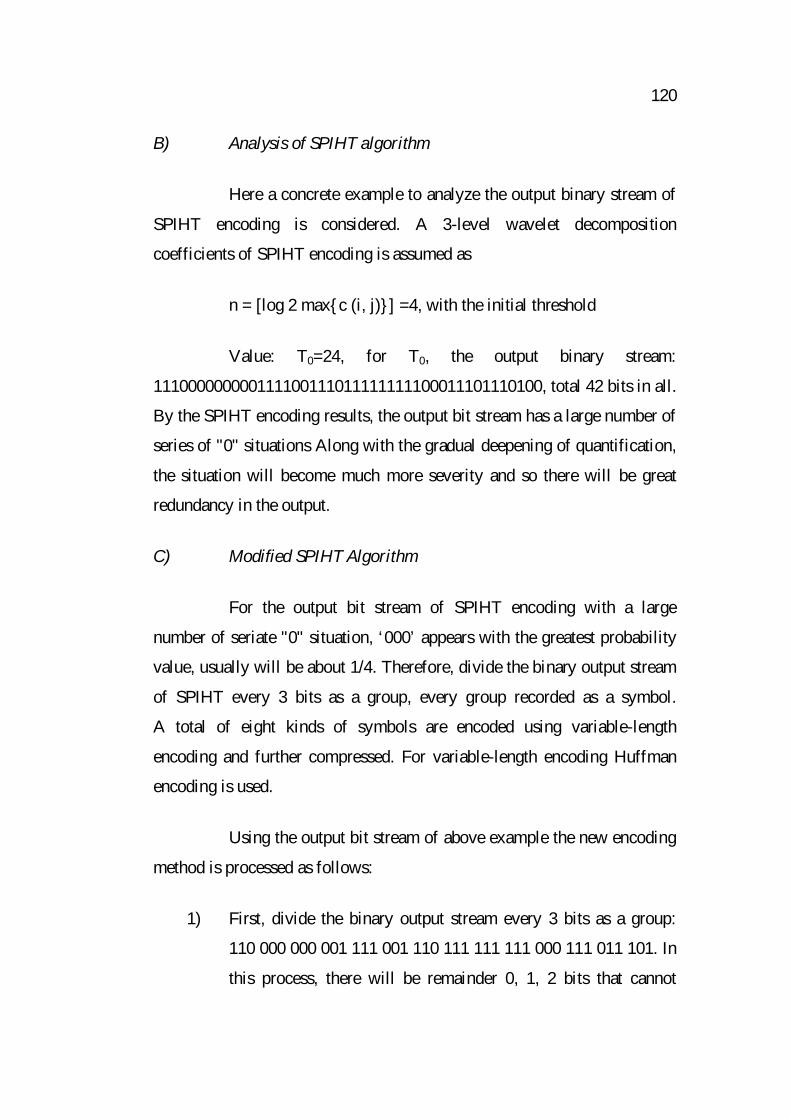
B) Analysis of SPIHT algorithm
Here a concrete example to analyze the output binary stream of
SPIHT encoding is considered. A 3-level wavelet decomposition
coefficients of SPIHT encoding is assumed as
n = [log 2 max{c (i, j)}] =4, with the initial threshold
Value: T0=24, for T0, the output binary stream:
111000000000111100111011111111100011101110100, total 42 bits in all.
By the SPIHT encoding results, the output bit stream has a large number of
series of "0" situations Along with the gradual deepening of quantification,
the situation will become much more severity and so there will be great
redundancy in the output.
C) Modified SPIHT Algorithm
For the output bit stream of SPIHT encoding with a large
number of seriate "0" situation, ‘000’ appears with the greatest probability
value, usually will be about 1/4. Therefore, divide the binary output stream
of SPIHT every 3 bits as a group, every group recorded as a symbol.
A total of eight kinds of symbols are encoded using variable-length
encoding and further compressed. For variable-length encoding Huffman
encoding is used.
Using the output bit stream of above example the new encoding
method is processed as follows:
1) First, divide the binary output stream every 3 bits as a group:
110 000 000 001 111 001 110 111 111 111 000 111 011 101. In
this process, there will be remainder 0, 1, 2 bits that cannot

121
participate. So, in order for unity, in the head of the output bit
stream of Huffman encoding cost ,two bits are used to record
the number of bits that do not participate in group and those
remainder bits arrive in the output at the end.
2) The emergence of statistical probability of each symbol
grouping results is as follows:
P (‘000’) = 0.2144 P (‘001’) =0.14
P (‘010’) = 0 P (‘011’) =0.07
P (‘100’) = 0 P (‘101’) = 0.07
P (‘110’) = 0.14 P (‘111’) = 0.35
3) According to the probability of the above results, using
Huffman encoding, code word book is obtained as shown in
Table 5.2.
Table 5.2 Code word comparison table
000 00 100 011
001 01 101 0011
010 11 110 01111
011 010 111 111111
Through the above code book ,one can get the corresponding
output stream as : 00 01 11 010 011 0011 01111 111111, a total of
27 bits. The ‘10’ in the head is binary of remainder bits’ number. The last
122
two bits ‘00’ are the result of directly outputting remainder bits. Compared
with the original bit stream 15 bits are saved. Decoding is the inverse
process of the above-mentioned scheme.
Decompression
This process is the reverse to the compression technique. After
SPIHT, it is necessary to transform data to the original domain (spatial
domain). To do this, the inverse fractional fourier transform is applied first
in columns and secondly in rows.
Proposed Algorithm
The proposed image compression technique is very effective in
overcoming the limitations of the wavelet transform based coding
techniques when applied to images with linear Curves. The steps involved
in the proposed approach are:
i. Represent the image data as intensity values of pixels in the
spatial co-ordinates.
ii. Apply nonsubsample contourlet Transform on the image matrix
and get the contourlet coefficients of the image.
iii. Quantize the available coefficients using dead zone quantization
algorithm.
iv. Hybrid SPIHT encoding algorithm with Huffman encoding on
the bit stream.
123
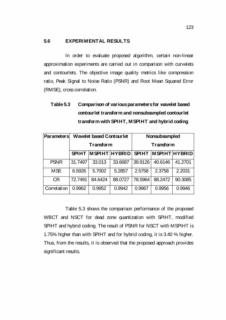
5.6 EXPERIMENTAL RESULTS
In order to evaluate proposed algorithm, certain non-linear
approximation experiments are carried out in comparison with curvelets
and contourlets. The objective image quality metrics like compression
ratio, Peak Signal to Noise Ratio (PSNR) and Root Mean Squared Error
(RMSE), cross correlation.
Table 5.3 Comparison of various parameters for wavelet based
contourlet transform and nonsubsampled contourlet
transform with SPIHT, MSPIHT and hybrid coding
Parameters Wavelet based Contourlet
Transform
Nonsubsampled
Transform
SPIHT MSPIHT HYBRID SPIHT MSPIHT HYBRID
PSNR 31.7497 33.013 33.6687 39.9126 40.6146 41.2701
MSE 6.5926 5.7002 5.2857 2.5758 2.3758 2.2031
CR 72.7491 84.6424 88.0727 78.5964 88.2472 90.3085
Correlation 0.9962 0.9952 0.9942 0.9967 0.9956 0.9946
Table 5.3 shows the comparison performance of the proposed
WBCT and NSCT for dead zone quantization with SPIHT, modified
SPIHT and hybrid coding. The result of PSNR for NSCT with MSPIHT is
1.75% higher than with SPIHT and for hybrid coding, it is 3.40 % higher.
Thus, from the results, it is observed that the proposed approach provides
significant results.

124
5.7 SUMMARY
This chapter clearly shows and discusses about the problems in
wavelet based contourlet transform. Due to the drawbacks of wavelet based
contourlet transform, proposed approach uses a nonsubsampled contourlet
transformation with dead zone quantization. Moreover, for the encoding
purpose, SPIHT, modified SPIHT and hybrid coding of MSPIHT with
Huffman coding are used.


![141 Chapter 3 - Shodhgangashodhganga.inflibnet.ac.in › bitstream › 10603 › 19076 › 10 › 10_chapt… · 141 Chapter 3 [1, 2-a] pyridin-3-yl] methanol Imp-5 Imp-7 3.2 Literature](https://img.pdfslide.us/doc/110x75/5f0306ab7e708231d4072ba4/141-chapter-3-a-bitstream-a-10603-a-19076-a-10-a-10chapt-141-chapter.jpg)