Embed Size (px)
Citation preview
GIS and Decision-Making
Work Site Alliance – Community Based GIS 1© 2000
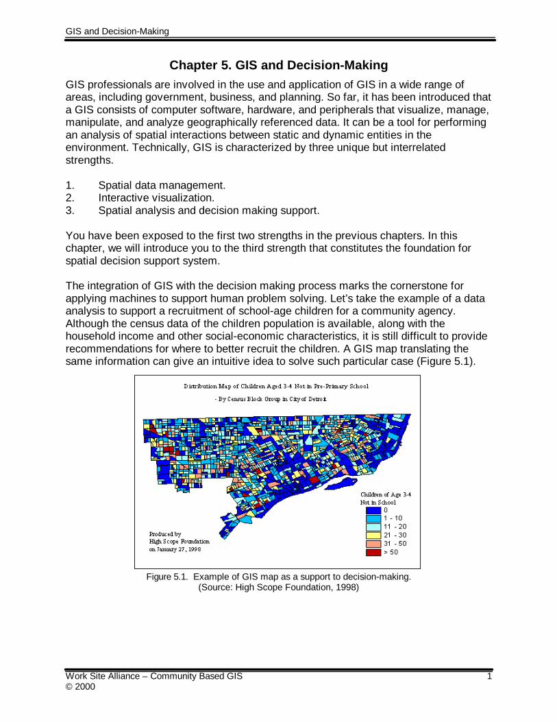
Chapter 5. GIS and Decision-MakingGIS professionals are involved in the use and application of GIS in a wide range ofareas, including government, business, and planning. So far, it has been introduced thata GIS consists of computer software, hardware, and peripherals that visualize, manage,manipulate, and analyze geographically referenced data. It can be a tool for performingan analysis of spatial interactions between static and dynamic entities in theenvironment. Technically, GIS is characterized by three unique but interrelatedstrengths.
1. Spatial data management.2. Interactive visualization.3. Spatial analysis and decision making support.
You have been exposed to the first two strengths in the previous chapters. In thischapter, we will introduce you to the third strength that constitutes the foundation forspatial decision support system.
The integration of GIS with the decision making process marks the cornerstone forapplying machines to support human problem solving. Let’s take the example of a dataanalysis to support a recruitment of school-age children for a community agency.Although the census data of the children population is available, along with thehousehold income and other social-economic characteristics, it is still difficult to providerecommendations for where to better recruit the children. A GIS map translating thesame information can give an intuitive idea to solve such particular case (Figure 5.1).
Figure 5.1. Example of GIS map as a support to decision-making.(Source: High Scope Foundation, 1998)
GIS and Decision-Making
Work Site Alliance – Community Based GIS 2© 2000
This chapter will continue the introduction of basic concepts and techniques of GIS insolving real-world problems. This chapter contains four sections:
Section 1: Spatial analysis and decision making support, which introduces theimportance of GIS spatial analysis.
Section 2: Basics of spatial analysis, which focuses on basic concepts, generalsteps, and types of spatial analysis.
Section 3: ArcView solutions for spatial analysis, which introduces how a desktopGIS handles spatial analysis, and how spatial analysis functions can beenhanced in a desktop GIS. Several exercises are designed to help youget familiar with spatial analysis in the context of answering some simplequestions.
Section 4: Exercises, which provides hands-on experience with spatial analysis invarious settings.
1. Spatial Analysis And Decision Making SupportDecision-making from spatial analysis involves four important considerations• An objective (as opposed to subjective) understanding of the reality; the
potential problem(s) must be clearly formulated and specified from thebeginning of the process.
• Some specific guideline(s) to base the future decision upon.• The availability of a data set for a modeling /quantitative analysis.• An awareness of the social and environmental constraints.
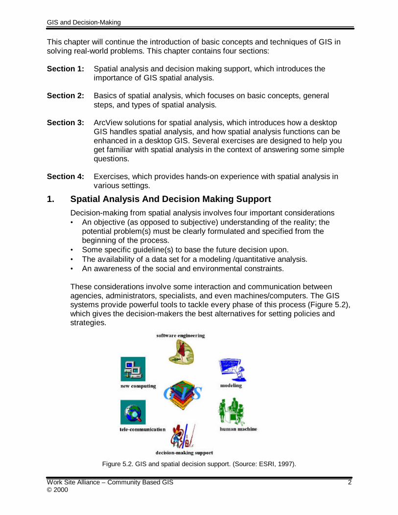
These considerations involve some interaction and communication betweenagencies, administrators, specialists, and even machines/computers. The GISsystems provide powerful tools to tackle every phase of this process (Figure 5.2),which gives the decision-makers the best alternatives for setting policies andstrategies.
Figure 5.2. GIS and spatial decision support. (Source: ESRI, 1997).
GIS and Decision-Making
Work Site Alliance – Community Based GIS 3© 2000
2. Basics of Spatial Analysis
Geographic analysis allows the study of real-world processes (which then can besimplified conceptually, qualitatively, quantitatively, or for administrative andpolitical purposes) by developing and applying models. A GIS provides valuabletools that can be combined in meaningful sequences to develop new models.Such models may reveal some underlying trends in the geographic data and mayprovide new valuable information; they may bring to the user’s attention new orpreviously unnoticed relationships within and between data sets, increasing theunderstanding of the real world.
2.1 General steps for performing Spatial Analysis
Before starting any GIS application or project, two key-questions must beaddressed: why and how.
Why gives the motivation for using a GIS system, indicating that you need toknow the problem you are trying to solve. You need to assess the problem athand and establish an objective.
How is organizing the needed logical steps and procedures to solve the problem.Spending sufficient time in figuring out the right steps to solve a problem is anecessity to GIS users. You should try to avoid launching GIS operations beforeknowing what outcomes will be generated. Though it is not trivial for a beginner,you need to think through the process, which will lead to the right solutions. It isimperative that you should know the following issues
• The problem(s).• The data.• Domain specific problem-solving rules.• Available GIS functions (supported by the GIS software you are using).
Though there is no fixed way of organizing a GIS project, the following steps arerecommend by the majority of GIS professionals (ESRI, 1995, p.8-2).
Step 1: Establish the objectives and criteria for the analysis.Step 2: Outline the procedures step by step based on the expert knowledge of
the problem to solve.Step 3: Define the right GIS operations (commands), and find the needed spatial
and tabular data, for the problem-solving procedures.Step 4: Prepare the data for spatial operations.Step 5: Perform the spatial operations.Step 6: Prepare the derived data for tabular analysis.Step 7: Perform the tabular analysis.Step 8: Evaluate and interpret the results.
GIS and Decision-Making
Work Site Alliance – Community Based GIS 4© 2000
Step 9: Refine the analysis as needed.
2.2 Types of Spatial AnalysisSpatial analysis includes a wide variety of GIS functions, ranging from simpletopological operations to more complex modeling or advanced statisticaloperations. However, topological operations account for the majority of spatialanalysis performed in ordinary GIS applications.
Some topological operations are frequently used; we have organized them intofour principal groups.
• Proximity analysis, such as, buffer, near, and point distance commands inArc/Info;Used when you need information about the area surrounding existingfeatures.
• Boundary operations, including “append”, “clip”, “erase”, “map join”, “split”,“update” functions;Used when the information you need can be selected by its geographiclocation.
• Logical operations, such as “reselect”, “dissolve/merge”, “eliminate”;Used when the information you want can be selected by its descriptiveattributes.
• Spatial joins, including, identity, intersect, union (all of these consisting ofGIS Overlay functionality);Used when you need to add polygon information from other geographicfeatures to your current database.
3. Examples of Spatial Analysis
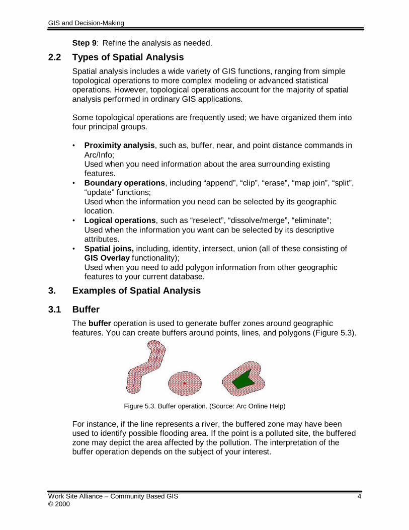
3.1 BufferThe buffer operation is used to generate buffer zones around geographicfeatures. You can create buffers around points, lines, and polygons (Figure 5.3).
Figure 5.3. Buffer operation. (Source: Arc Online Help)
For instance, if the line represents a river, the buffered zone may have beenused to identify possible flooding area. If the point is a polluted site, the bufferedzone may depict the area affected by the pollution. The interpretation of thebuffer operation depends on the subject of your interest.
GIS and Decision-Making
Work Site Alliance – Community Based GIS 5© 2000
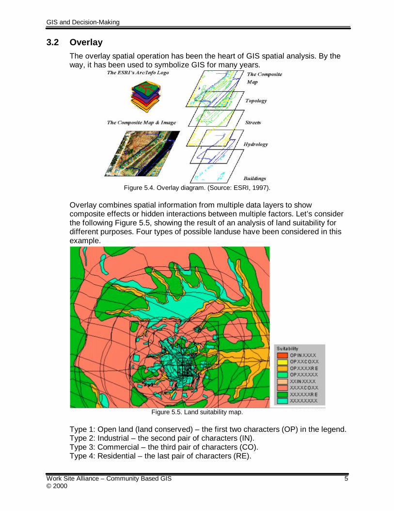
3.2 OverlayThe overlay spatial operation has been the heart of GIS spatial analysis. By theway, it has been used to symbolize GIS for many years.
Figure 5.4. Overlay diagram. (Source: ESRI, 1997).
Overlay combines spatial information from multiple data layers to showcomposite effects or hidden interactions between multiple factors. Let’s considerthe following Figure 5.5, showing the result of an analysis of land suitability fordifferent purposes. Four types of possible landuse have been considered in thisexample.
Figure 5.5. Land suitability map.
Type 1: Open land (land conserved) – the first two characters (OP) in the legend.Type 2: Industrial – the second pair of characters (IN).Type 3: Commercial – the third pair of characters (CO).Type 4: Residential – the last pair of characters (RE).
GIS and Decision-Making
Work Site Alliance – Community Based GIS 6© 2000
The XX annotation is attributed to lands that do not fit into any of these giventypes.
The purpose, in this example, is to decide about the suitability of an area for aspecific landuse. This logical reasoning is built on the GIS operation overlay. Ingeneral, the analysis involves three main steps as follow.
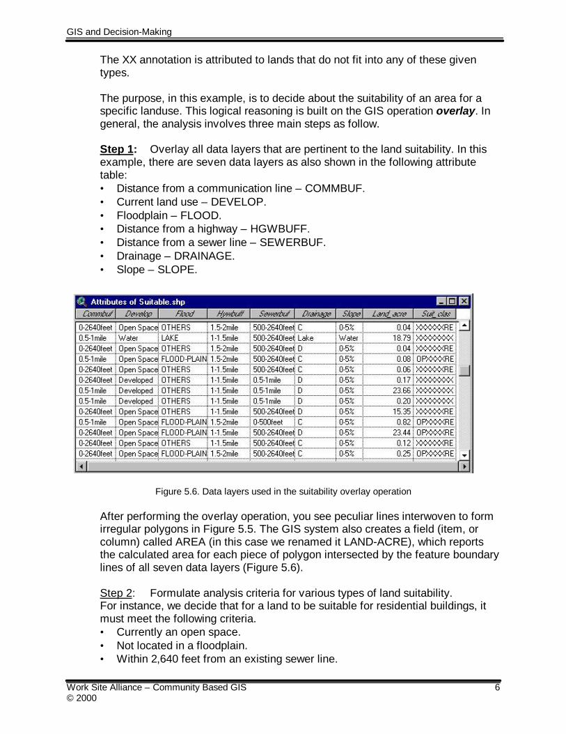
Step 1: Overlay all data layers that are pertinent to the land suitability. In thisexample, there are seven data layers as also shown in the following attributetable:• Distance from a communication line – COMMBUF.• Current land use – DEVELOP.• Floodplain – FLOOD.• Distance from a highway – HGWBUFF.• Distance from a sewer line – SEWERBUF.• Drainage – DRAINAGE.• Slope – SLOPE.
Figure 5.6. Data layers used in the suitability overlay operation
After performing the overlay operation, you see peculiar lines interwoven to formirregular polygons in Figure 5.5. The GIS system also creates a field (item, orcolumn) called AREA (in this case we renamed it LAND-ACRE), which reportsthe calculated area for each piece of polygon intersected by the feature boundarylines of all seven data layers (Figure 5.6).
Step 2: Formulate analysis criteria for various types of land suitability.For instance, we decide that for a land to be suitable for residential buildings, itmust meet the following criteria.• Currently an open space.• Not located in a floodplain.• Within 2,640 feet from an existing sewer line.
GIS and Decision-Making
Work Site Alliance – Community Based GIS 7© 2000
• Landscape slope cannot exceed 5%.
A similar approach can be taken to define suitability for other land uses.
Step 3: Apply the criteria to your data sets (through query or reselect) toidentify the suitability for each piece of land (see Column, SUIT_CLAS in Figure5.6).
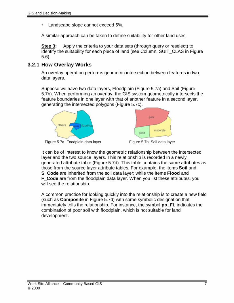
3.2.1 How Overlay WorksAn overlay operation performs geometric intersection between features in twodata layers.
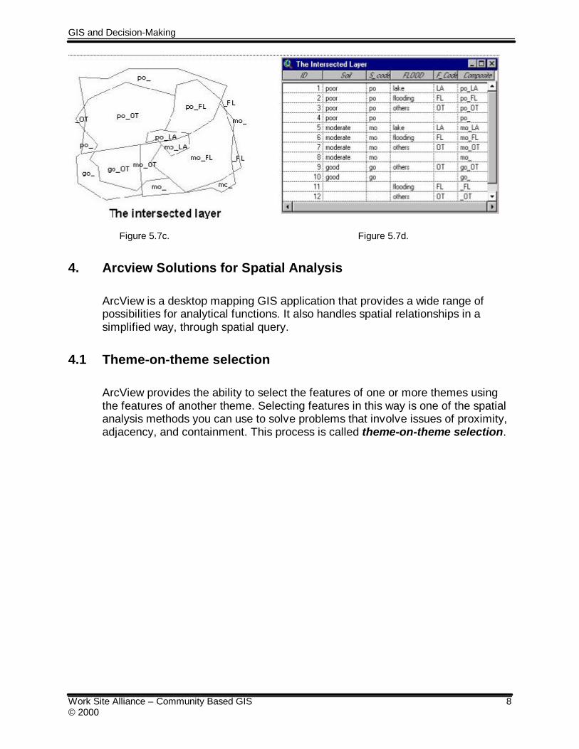
Suppose we have two data layers, Floodplain (Figure 5.7a) and Soil (Figure5.7b). When performing an overlay, the GIS system geometrically intersects thefeature boundaries in one layer with that of another feature in a second layer,generating the intersected polygons (Figure 5.7c).
Figure 5.7a. Foodplain data layer Figure 5.7b. Soil data layer
It can be of interest to know the geometric relationship between the intersectedlayer and the two source layers. This relationship is recorded in a newlygenerated attribute table (Figure 5.7d). This table contains the same attributes asthose from the source layer attribute tables. For example, the items Soil andS_Code are inherited from the soil data layer; while the items Flood andF_Code are from the floodplain data layer. When you list these attributes, youwill see the relationship.
A common practice for looking quickly into the relationship is to create a new field(such as Composite in Figure 5.7d) with some symbolic designation thatimmediately tells the relationship. For instance, the symbol po_FL indicates thecombination of poor soil with floodplain, which is not suitable for landdevelopment.
GIS and Decision-Making
Work Site Alliance – Community Based GIS 8© 2000
Figure 5.7c. Figure 5.7d.
4. Arcview Solutions for Spatial Analysis
ArcView is a desktop mapping GIS application that provides a wide range ofpossibilities for analytical functions. It also handles spatial relationships in asimplified way, through spatial query.
4.1 Theme-on-theme selection
ArcView provides the ability to select the features of one or more themes usingthe features of another theme. Selecting features in this way is one of the spatialanalysis methods you can use to solve problems that involve issues of proximity,adjacency, and containment. This process is called theme-on-theme selection.
GIS and Decision-Making
Work Site Alliance – Community Based GIS 9© 2000
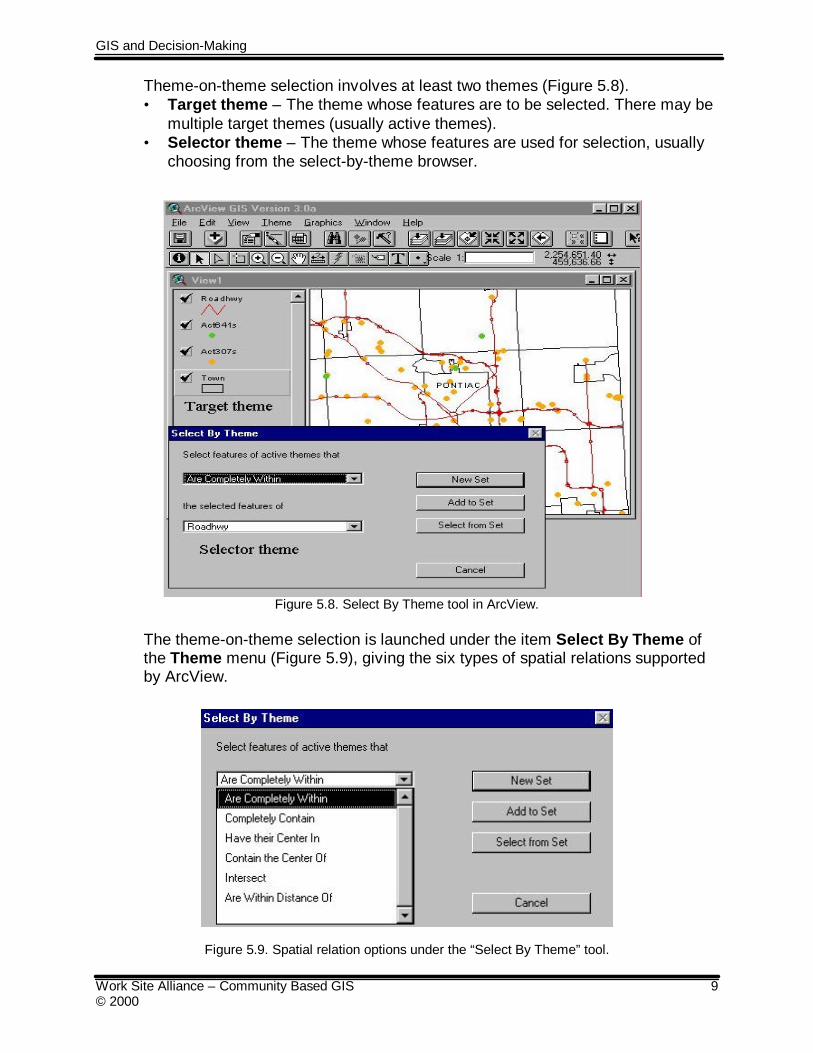
Theme-on-theme selection involves at least two themes (Figure 5.8).• Target theme – The theme whose features are to be selected. There may be
multiple target themes (usually active themes).• Selector theme – The theme whose features are used for selection, usually
choosing from the select-by-theme browser.
Figure 5.8. Select By Theme tool in ArcView.
The theme-on-theme selection is launched under the item Select By Theme ofthe Theme menu (Figure 5.9), giving the six types of spatial relations supportedby ArcView.
Figure 5.9. Spatial relation options under the “Select By Theme” tool.
GIS and Decision-Making
Work Site Alliance – Community Based GIS 10© 2000
Are Completely Within - Selects features in the target themes if they fallcompletely within one or more of the selector theme's features.
Completely Contain - Selects features in the target themes that completelycontain one or more of the selector theme's features.
Have their Center In - Selects features in the target themes if their center fallsinside the selector theme's features.
Contain the Center Of - Selects features in the target themes that contain thecenter of one or more of the selector theme's features
Intersect - Selects features in the target themes that intersect the features in thetarget. Intersection implies that at least one point is common to both the selectorand the target or one of them is completely within the other. If the selector andtarget are the same, Intersect will select adjacent features.
Are Within Distance Of - Selects features in the target themes that are within aspecified distance of the selector theme's features.
4.2 Spatial JoinSpatial join is another spatial analysis method (see paragraph 2.2 of thisChapter). It is set to define possible relationship(s) among points and polygons(defined in paragraph 1 of Chapter 2).
A spatial join functions much like an attribute join on two tables, but thedifference resides in that it uses the Shape fields to join the attribute tables,whereas the table join uses any other common field to the two tables (seeExercise 4C of Chapter 4). ArcView supports the following spatial joins.• Point to Point (proximity)• Point to Line (proximity)• Point in Polygon (inclusion)• Line to Point (proximity)• Line in Line (intersection)• Line in Polygon (inclusion)• Polygon in Polygon (inclusion)
Spatial queries can also be used to define some specific relationship betweenthemes; for example, to identify students in a particular school district area, tolocate zip codes within school districts, to trace bus routes within school districts,or a variety of other possibilities related to spatial data (Ibid). In a spatial join,three types of spatial relations are used. Depending on the theme types, you willuse different spatial relations. For Point in Polygon, Line in Polygon, and Polygonin Polygon joins, you will use the “Are Completely Within” spatial relation type.For example, assume you want to join two polygon themes, one for zip codes,and one for school districts. The zip codes table is the destination attribute table.The only zip codes to receive school district attributes following the spatial joinare those that are contained entirely within a single school district area.
GIS and Decision-Making
Work Site Alliance – Community Based GIS 11© 2000
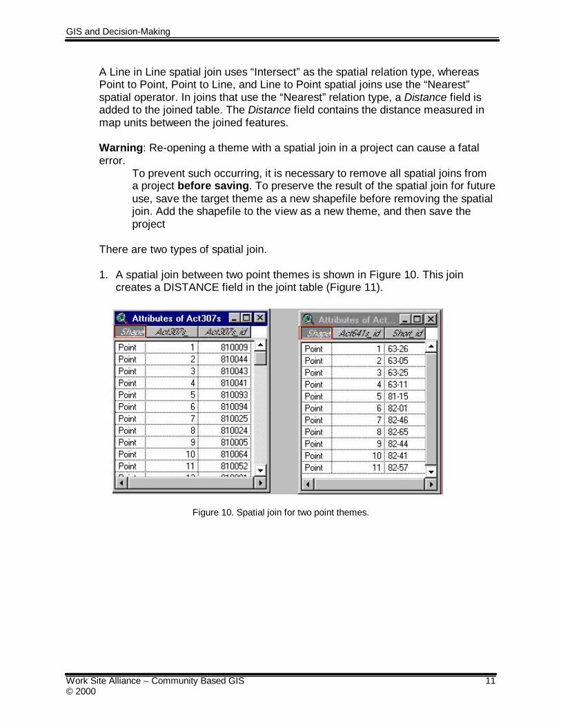
A Line in Line spatial join uses “Intersect” as the spatial relation type, whereasPoint to Point, Point to Line, and Line to Point spatial joins use the “Nearest”spatial operator. In joins that use the “Nearest” relation type, a Distance field isadded to the joined table. The Distance field contains the distance measured inmap units between the joined features.
Warning: Re-opening a theme with a spatial join in a project can cause a fatalerror.
To prevent such occurring, it is necessary to remove all spatial joins froma project before saving. To preserve the result of the spatial join for futureuse, save the target theme as a new shapefile before removing the spatialjoin. Add the shapefile to the view as a new theme, and then save theproject
There are two types of spatial join.
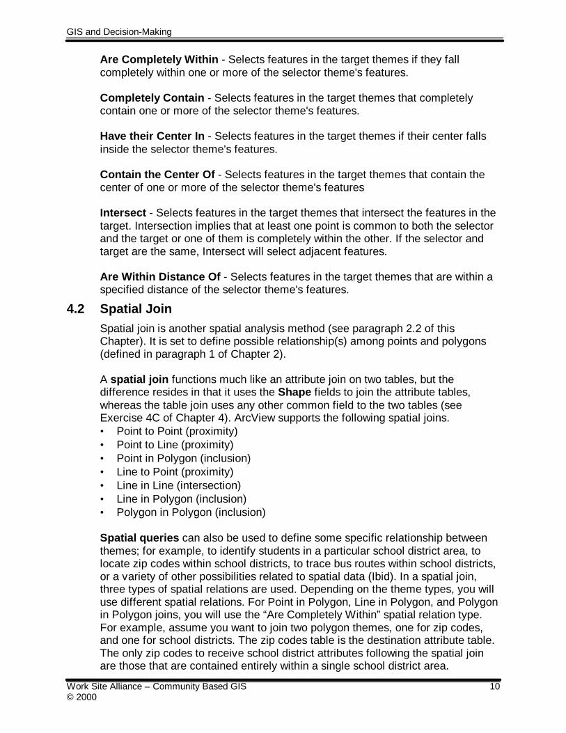
1. A spatial join between two point themes is shown in Figure 10. This joincreates a DISTANCE field in the joint table (Figure 11).
Figure 10. Spatial join for two point themes.
GIS and Decision-Making
Work Site Alliance – Community Based GIS 12© 2000
Figure 11. Results of a spatial join between two point themes.
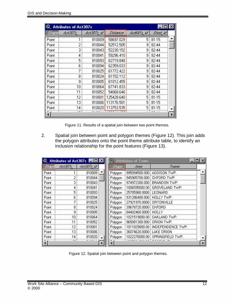
2. Spatial join between point and polygon themes (Figure 12). This join addsthe polygon attributes onto the point theme attribute table, to identify aninclusion relationship for the point features (Figure 13).
Figure 12. Spatial join between point and polygon themes.
GIS and Decision-Making
Work Site Alliance – Community Based GIS 13© 2000
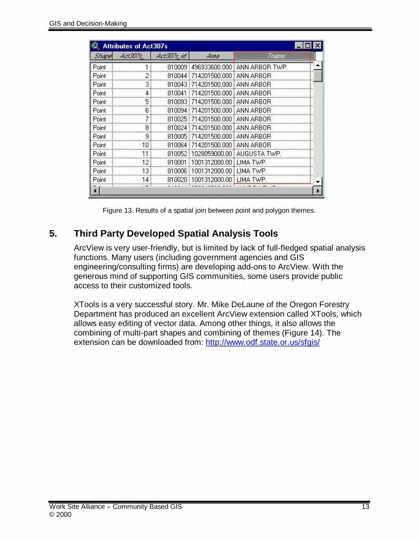
Figure 13. Results of a spatial join between point and polygon themes.
5. Third Party Developed Spatial Analysis ToolsArcView is very user-friendly, but is limited by lack of full-fledged spatial analysisfunctions. Many users (including government agencies and GISengineering/consulting firms) are developing add-ons to ArcView. With thegenerous mind of supporting GIS communities, some users provide publicaccess to their customized tools.
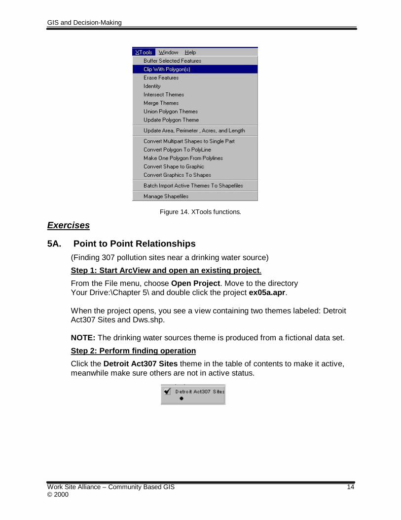
XTools is a very successful story. Mr. Mike DeLaune of the Oregon ForestryDepartment has produced an excellent ArcView extension called XTools, whichallows easy editing of vector data. Among other things, it also allows thecombining of multi-part shapes and combining of themes (Figure 14). Theextension can be downloaded from: http://www.odf.state.or.us/sfgis/
GIS and Decision-Making
Work Site Alliance – Community Based GIS 14© 2000
Figure 14. XTools functions.
Exercises
5A. Point to Point Relationships(Finding 307 pollution sites near a drinking water source)
Step 1: Start ArcView and open an existing project.
From the File menu, choose Open Project. Move to the directoryYour Drive:\Chapter 5\ and double click the project ex05a.apr.
When the project opens, you see a view containing two themes labeled: DetroitAct307 Sites and Dws.shp.
NOTE: The drinking water sources theme is produced from a fictional data set.
Step 2: Perform finding operation
Click the Detroit Act307 Sites theme in the table of contents to make it active,meanwhile make sure others are not in active status.
GIS and Decision-Making
Work Site Alliance – Community Based GIS 15© 2000
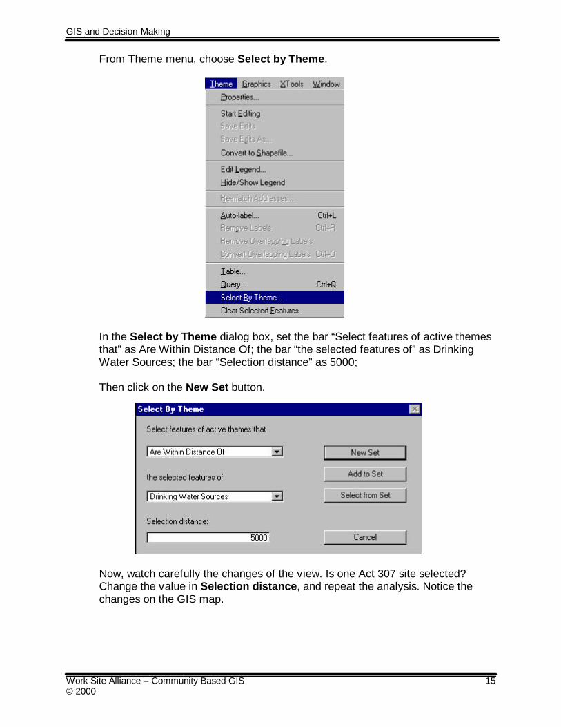
From Theme menu, choose Select by Theme.
In the Select by Theme dialog box, set the bar “Select features of active themesthat” as Are Within Distance Of; the bar “the selected features of” as DrinkingWater Sources; the bar “Selection distance” as 5000;
Then click on the New Set button.
Now, watch carefully the changes of the view. Is one Act 307 site selected?Change the value in Selection distance, and repeat the analysis. Notice thechanges on the GIS map.
GIS and Decision-Making
Work Site Alliance – Community Based GIS 16© 2000
Step 3: Save and close the project
Make the Project window active.From the File menu, choose Save Project As.Give a name to your project.Move to your personal directory and save the project.From the File menu, choose Close Project.
5B. Point to Line Relationships
Step 1: Start ArcView and open an existing project
From the File menu, choose Open Project. Move to the directoryYour Drive:\Chapter 5\ and double click the project ex05b.apr.
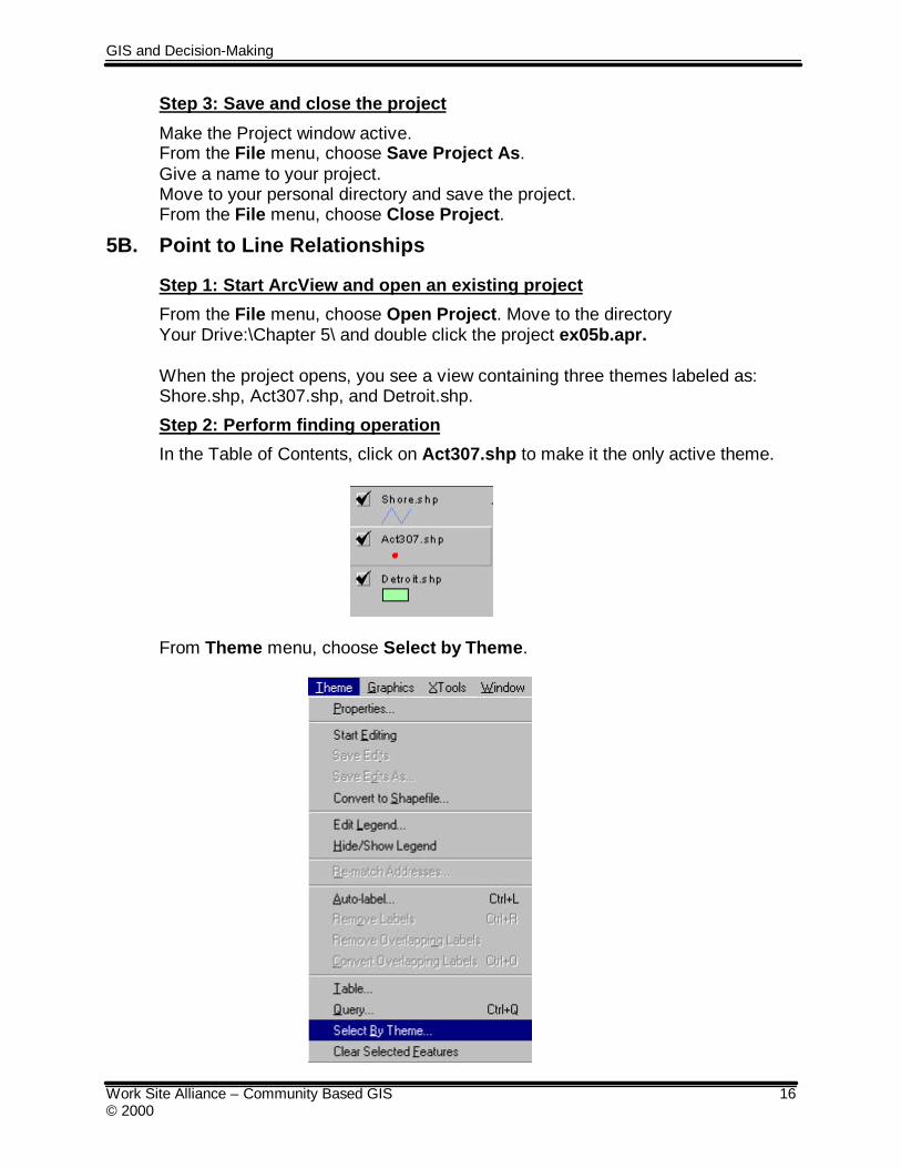
When the project opens, you see a view containing three themes labeled as:Shore.shp, Act307.shp, and Detroit.shp.
Step 2: Perform finding operation
In the Table of Contents, click on Act307.shp to make it the only active theme.
From Theme menu, choose Select by Theme.
GIS and Decision-Making
Work Site Alliance – Community Based GIS 17© 2000
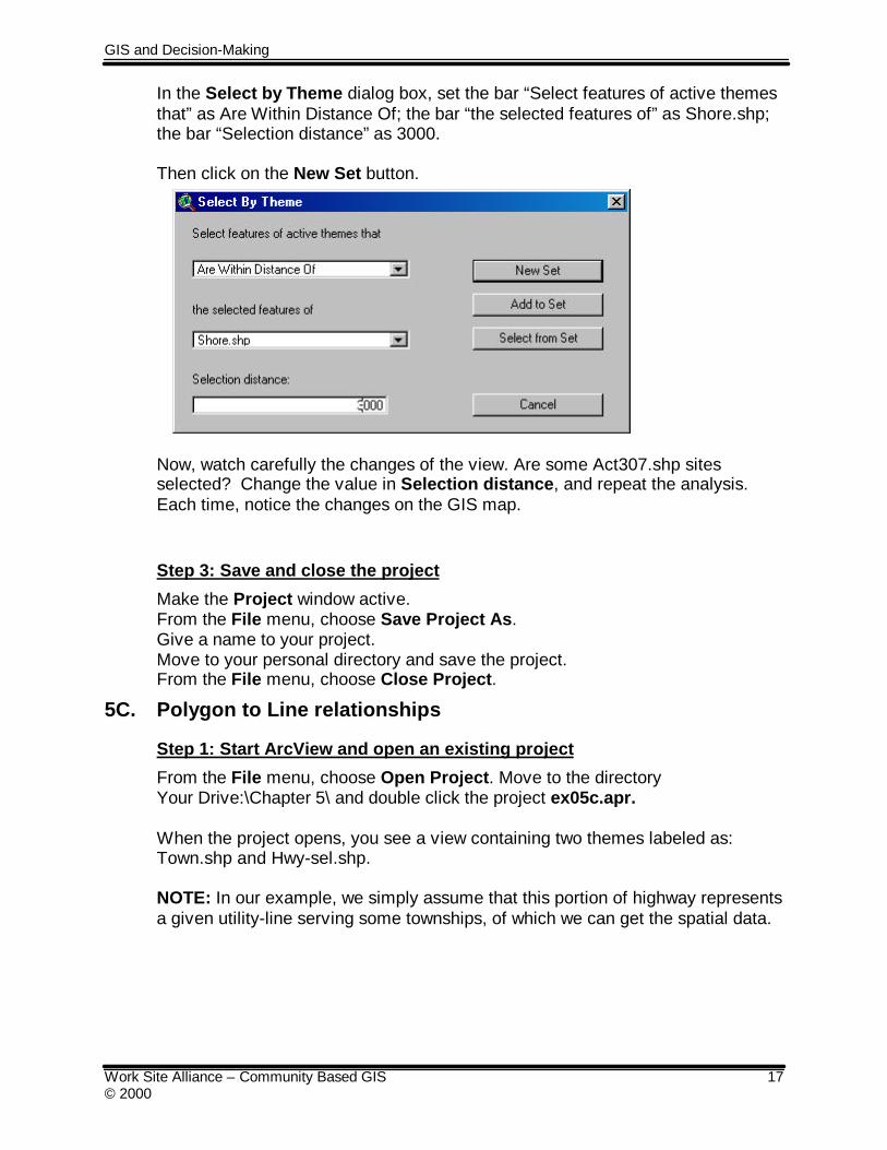
In the Select by Theme dialog box, set the bar “Select features of active themesthat” as Are Within Distance Of; the bar “the selected features of” as Shore.shp;the bar “Selection distance” as 3000.
Then click on the New Set button.
Now, watch carefully the changes of the view. Are some Act307.shp sitesselected? Change the value in Selection distance, and repeat the analysis.Each time, notice the changes on the GIS map.
Step 3: Save and close the project
Make the Project window active.From the File menu, choose Save Project As.Give a name to your project.Move to your personal directory and save the project.From the File menu, choose Close Project.
5C. Polygon to Line relationships
Step 1: Start ArcView and open an existing project
From the File menu, choose Open Project. Move to the directoryYour Drive:\Chapter 5\ and double click the project ex05c.apr.
When the project opens, you see a view containing two themes labeled as:Town.shp and Hwy-sel.shp.
NOTE: In our example, we simply assume that this portion of highway representsa given utility-line serving some townships, of which we can get the spatial data.
GIS and Decision-Making
Work Site Alliance – Community Based GIS 18© 2000
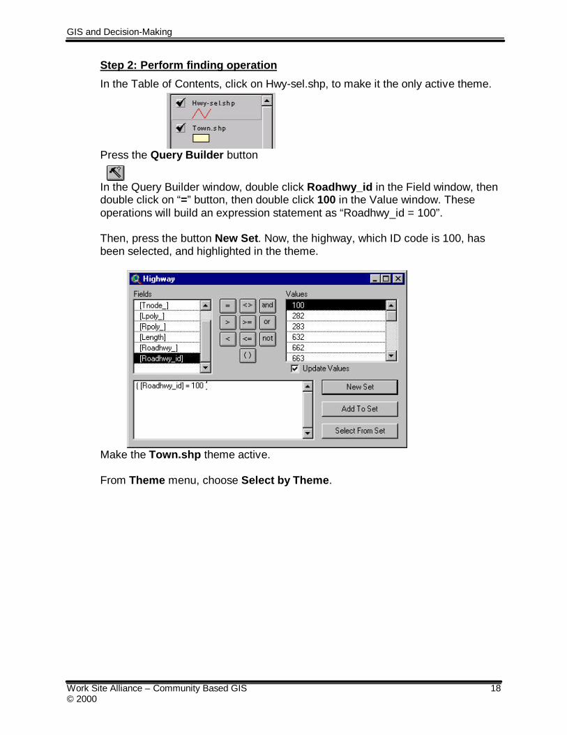
Step 2: Perform finding operation
In the Table of Contents, click on Hwy-sel.shp, to make it the only active theme.
Press the Query Builder button
In the Query Builder window, double click Roadhwy_id in the Field window, thendouble click on “=” button, then double click 100 in the Value window. Theseoperations will build an expression statement as “Roadhwy_id = 100”.
Then, press the button New Set. Now, the highway, which ID code is 100, hasbeen selected, and highlighted in the theme.
Make the Town.shp theme active.
From Theme menu, choose Select by Theme.
GIS and Decision-Making
Work Site Alliance – Community Based GIS 19© 2000
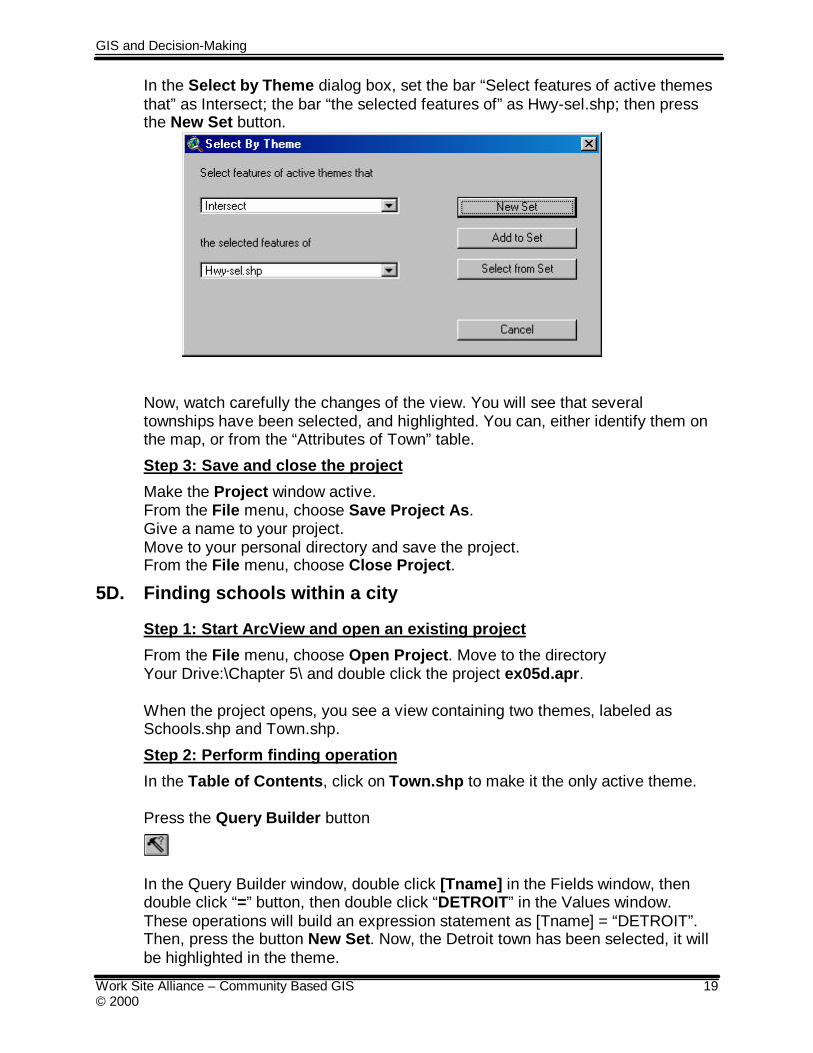
In the Select by Theme dialog box, set the bar “Select features of active themesthat” as Intersect; the bar “the selected features of” as Hwy-sel.shp; then pressthe New Set button.
Now, watch carefully the changes of the view. You will see that severaltownships have been selected, and highlighted. You can, either identify them onthe map, or from the “Attributes of Town” table.
Step 3: Save and close the project
Make the Project window active.From the File menu, choose Save Project As.Give a name to your project.Move to your personal directory and save the project.From the File menu, choose Close Project.
5D. Finding schools within a city
Step 1: Start ArcView and open an existing project
From the File menu, choose Open Project. Move to the directoryYour Drive:\Chapter 5\ and double click the project ex05d.apr.
When the project opens, you see a view containing two themes, labeled asSchools.shp and Town.shp.
Step 2: Perform finding operation
In the Table of Contents, click on Town.shp to make it the only active theme.
Press the Query Builder button
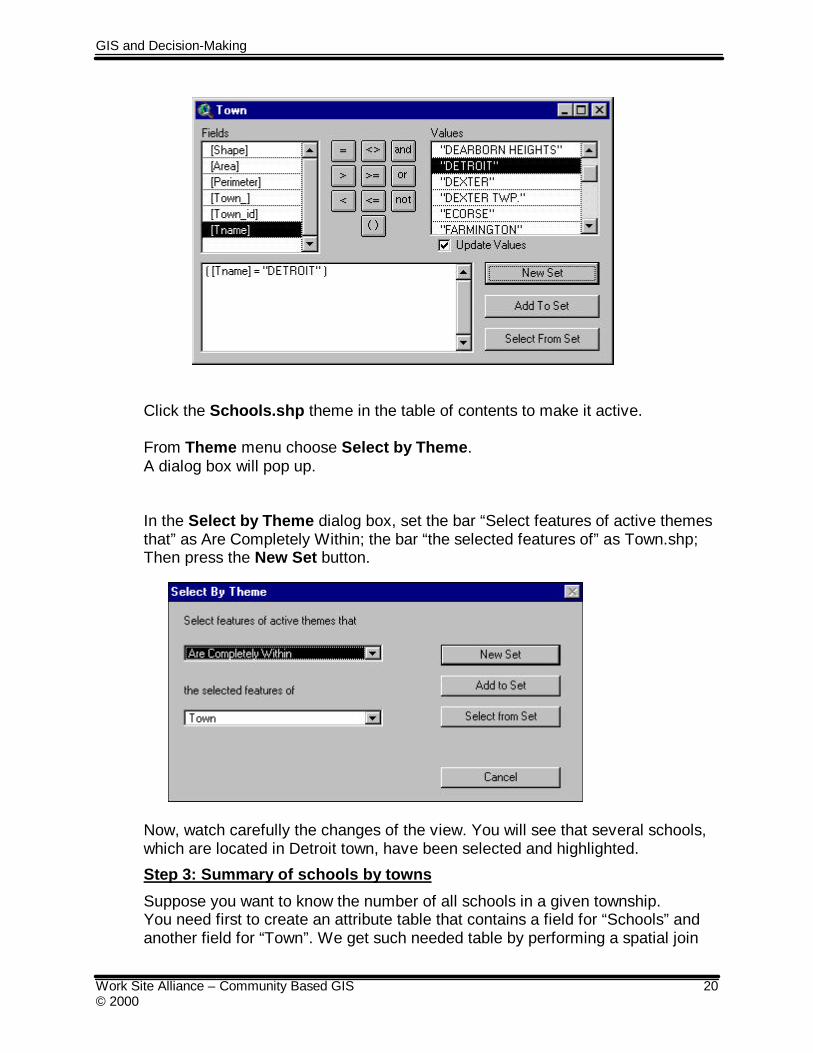
In the Query Builder window, double click [Tname] in the Fields window, thendouble click “=” button, then double click “DETROIT” in the Values window.These operations will build an expression statement as [Tname] = “DETROIT”.Then, press the button New Set. Now, the Detroit town has been selected, it willbe highlighted in the theme.
GIS and Decision-Making
Work Site Alliance – Community Based GIS 20© 2000
Click the Schools.shp theme in the table of contents to make it active.
From Theme menu choose Select by Theme.A dialog box will pop up.
In the Select by Theme dialog box, set the bar “Select features of active themesthat” as Are Completely Within; the bar “the selected features of” as Town.shp;Then press the New Set button.
Now, watch carefully the changes of the view. You will see that several schools,which are located in Detroit town, have been selected and highlighted.
Step 3: Summary of schools by towns
Suppose you want to know the number of all schools in a given township.You need first to create an attribute table that contains a field for “Schools” andanother field for “Town”. We get such needed table by performing a spatial join
GIS and Decision-Making
Work Site Alliance – Community Based GIS 21© 2000
between the attribute tables corresponding to the actual themes. With theresulting table, you then summarize as in Step 3 of Exercise 4B.
• With the Towns.shp theme active, open the table Attributes of Town.shp.Click on the field Shape.
With the Schools.shp theme active, open now the table Attributes ofSchools.shp.Click on the field Shape.
Click on the Join button to create a spatial join between the two tables.A single table is created, containing all the fields from the two previouslyseparate tables.
• Keep the Schools.shp theme as the active one.In the “joined” table, click on the Tname field to make it active.
Click the Summarize button to open the Summary Table Definitiondialog box.
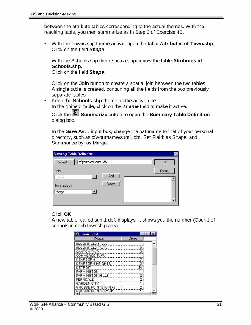
In the Save As… input box, change the pathname to that of your personaldirectory, such as c:\yourname\sum1.dbf. Set Field: as Shape, andSummarize by: as Merge.
Click OKA new table, called sum1.dbf, displays. It shows you the number (Count) ofschools in each township area.
GIS and Decision-Making
Work Site Alliance – Community Based GIS 22© 2000
Important Note: It is important to REMOVE ALL JOINS in the attribute tablebefore you continue.Make the Attributes of Schools.shp table active. Click on Remove All Joins,under the Table menu.
Step 4: Legend the towns theme by the total number of schools
In this step, you will put on the map the number of schools as a legend for eachtownship polygon. (The map in the View document will show the numbers ofschool in each township polygon, allowing a quick visual of the existing situationin the area).
Keep the sum1.dbf table from the previous Step 3 open.Click on the Tname field to make it active.
Open the table Attributes of Town.shp.Click on the Tname field to make it active.
Join the two tables.
Make the Towns.shp theme active.
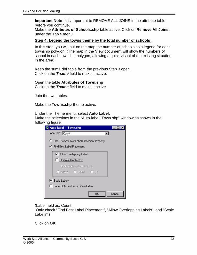
Under the Theme menu, select Auto Label.Make the selections in the “Auto-label: Town.shp” window as shown in thefollowing figure:
(Label field as: Count Only check “Find Best Label Placement”, “Allow Overlapping Labels”, and “ScaleLabels”.)
Click on OK.

GIS and Decision-Making
Work Site Alliance – Community Based GIS 23© 2000
Step 5: Save and close the project
Make the Project window active. From the File menu, choose Save Project As.Give a name to your project.
Move to your personal directory and save the project.From the File menu, choose Close Project.

GIS and Decision-Making
Work Site Alliance – Community Based GIS 24© 2000
Bibliography
Environmental Systems Research Institute, 1998. ARC/INFO Online Help.
High Scope Foundation, 1998. Distribution of Children Ages 3-4 Not in Pre-PrimarySchool.