Chapter 4 THE STRUCTURE AND ENERGY OF GRAIN BOUNDARIESusers.encs.concordia.ca/~mmedraj/tmg-books... · 2007-08-14 · Chapter 4 THE STRUCTURE AND ENERGY OF GRAIN BOUNDARIES 4.1 INTRODUCTION

Chapter 4

THE STRUCTURE ANDENERGY OF GRAINBOUNDARIES

4.1 INTRODUCTION

The majority of the book is concerned with the ways in which boundaries separatingregions of different crystallographic orientation are formed or are rearranged onannealing either during or after deformation. In this chapter we will introduce someaspects of the structure and properties of these boundaries and in chapter 5 we discussthe migration and the mobility of boundaries. We will concentrate on those aspects ofgrain boundaries which are most relevant to recovery, recrystallization and graingrowth and will not attempt to give a full coverage of the subject. Further informationon grain boundaries may be found in the books by Hirth and Lothe (1968), Bollmann(1970), Gleiter and Chalmers (1972), Chadwick and Smith (1976), Balluffi (1980), Wolfand Yip (1992), Sutton and Balluffi (1995) and Gottstein and Shvindlerman (1999).

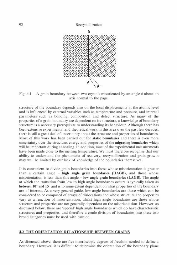
If we consider a grain boundary such as that shown in figure 4.1, the overall geometry ofthe boundary is defined by the orientation of the boundary plane AB with respect to oneof the two crystals (two degrees of freedom) and by the smallest rotation (�) required tomake the two crystals coincident (three degrees of freedom). There are thus five

macroscopic degrees of freedom which define the geometry of the boundary. In additionto this, the boundary structure is dependent on three microscopic degrees of freedom,

which are the rigid body translations parallel and perpendicular to the boundary. The

91

structure of the boundary depends also on the local displacements at the atomic leveland is influenced by external variables such as temperature and pressure, and internalparameters such as bonding, composition and defect structure. As many of theproperties of a grain boundary are dependent on its structure, a knowledge of boundarystructure is a necessary prerequisite to understanding its behaviour. Although there hasbeen extensive experimental and theoretical work in this area over the past few decades,there is still a great deal of uncertainty about the structure and properties of boundaries.Most of this work has been carried out for static boundaries and there is even moreuncertainty over the structure, energy and properties of the migrating boundaries whichwill be important during annealing. In addition, most of the experimental measurementshave been made close to the melting temperature. We must therefore recognise that ourability to understand the phenomena of recovery, recrystallization and grain growthmay well be limited by our lack of knowledge of the boundaries themselves.

It is convenient to divide grain boundaries into those whose misorientation is greaterthan a certain angle – high angle grain boundaries (HAGB), and those whosemisorientation is less than this angle – low angle grain boundaries (LAGB). The angleat which the transition from low to high angle boundaries occurs is typically taken asbetween 10� and 15� and is to some extent dependent on what properties of the boundaryare of interest. As a very general guide, low angle boundaries are those which can beconsidered to be composed of arrays of dislocations and whose structure and propertiesvary as a function of misorientation, whilst high angle boundaries are those whosestructure and properties are not generally dependent on the misorientation. However, asdiscussed below, there are ‘special’ high angle boundaries which do have characteristicstructures and properties, and therefore a crude division of boundaries into these twobroad categories must be used with caution.

4.2 THE ORIENTATION RELATIONSHIP BETWEEN GRAINS

As discussed above, there are five macroscopic degrees of freedom needed to define aboundary. However, it is difficult to determine the orientation of the boundary plane

Fig. 4.1. A grain boundary between two crystals misoriented by an angle � about anaxis normal to the page.

92 Recrystallization

experimentally (§A2.6.3), and in many cases, we neglect it and consider only the threeparameters which define the orientation between the two grains adjacent to a boundary.It should however be recognised that the use of such an incomplete description of a

boundary may cause problems in the interpretation of boundary behaviour.

The relative orientation of two cubic crystals is formally described by the rotation of onecrystal which brings it into the same orientation as the other crystal. This may bedefined by the rotation matrix

R ¼

a11 a12 a13a21 a22 a23a31 a32 a33

24

35 ð4:1Þ

where aij are column vectors of direction cosines between the cartesian axes. The sums ofthe squares of each row and of each column are unity, the dot products between columnvectors are zero, so only three independent parameters are involved. The rotation angle(h) is given by

2cos� þ 1 ¼ a11þ a22þ a33 ð4:2Þ

and the direction of the rotation axis [uvw] is given by

½ða32� a23Þ, ða13� a31Þ, ða21� a12Þ�: ð4:3Þ

In cubic materials, because of the symmetry, the relative orientations of two grains canbe described in 24 different ways. In the absence of any special symmetry, it isconventional to describe the rotation by the angle/axis pair associated with the smallest

misorientation angle, and this is sometimes called the disorientation. The range of �which can occur is therefore limited, and Mackenzie (1958) has shown that themaximum value of � is 45� for <100>, 60� for <111>, 60.72� for <110> and amaximum of 62.8� for <1,1,

p2�1>. For a polycrystal containing grains of random

orientation, the distribution of � is as shown in figure 4.2, with a mean of 40�.

It should be emphasised that the misorientation distribution shown in figure 4.2 willonly occur for a random grain assembly, and that a non-random distribution oforientations (i.e. a crystallographic texture) such as is normally found afterthermomechanical processing, will alter the misorientation distribution. Examples ofthis are found in strongly textured material where the large volume of similarly orientedgrains results in a large number of low/medium angle boundaries (e.g. figs. 14.3a, andA2.1), and in materials containing large numbers of special boundaries (i.e. thecoincidence site boundaries discussed in §4.4.1) as shown in figure 11.8.

Figure 4.2 shows the distribution of misorientation angles regardless of themisorientation axes. However, if proximity to a specific misorientation axis is specified,the distribution may be markedly altered. For example figure 4.3 shows the distributionof misorientation angles predicted for a randomly oriented grain assembly in which onlythe axes closest to <110> are considered. The curve now shows two peaks, and asdemonstrated by Hutchinson et al. (1996), experimental observation of such peaks may

The Structure and Energy of Grain Boundaries 93

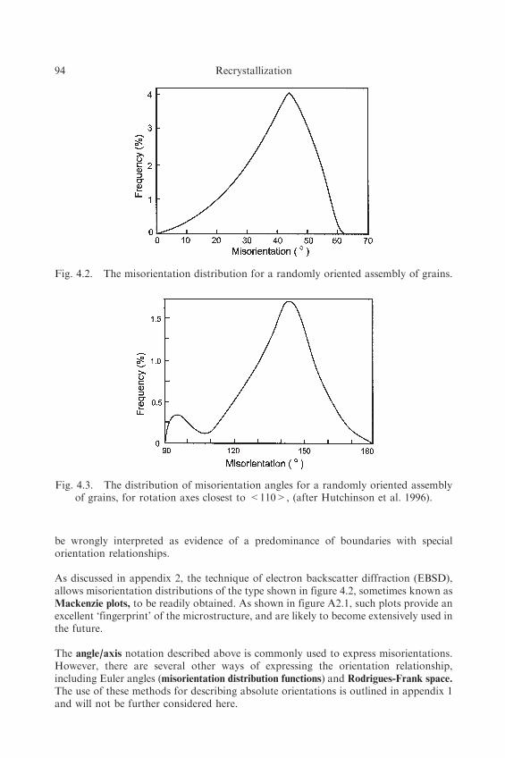
be wrongly interpreted as evidence of a predominance of boundaries with specialorientation relationships.

As discussed in appendix 2, the technique of electron backscatter diffraction (EBSD),allows misorientation distributions of the type shown in figure 4.2, sometimes known asMackenzie plots, to be readily obtained. As shown in figure A2.1, such plots provide anexcellent ‘fingerprint’ of the microstructure, and are likely to become extensively used inthe future.

The angle/axis notation described above is commonly used to express misorientations.However, there are several other ways of expressing the orientation relationship,including Euler angles (misorientation distribution functions) and Rodrigues-Frank space.

The use of these methods for describing absolute orientations is outlined in appendix 1and will not be further considered here.

Fig. 4.3. The distribution of misorientation angles for a randomly oriented assemblyof grains, for rotation axes closest to <110>, (after Hutchinson et al. 1996).

Fig. 4.2. The misorientation distribution for a randomly oriented assembly of grains.


4.3 LOW ANGLE GRAIN BOUNDARIES

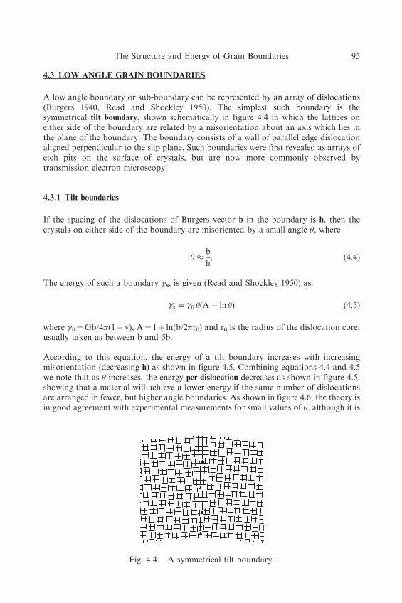
A low angle boundary or sub-boundary can be represented by an array of dislocations(Burgers 1940, Read and Shockley 1950). The simplest such boundary is thesymmetrical tilt boundary, shown schematically in figure 4.4 in which the lattices oneither side of the boundary are related by a misorientation about an axis which lies inthe plane of the boundary. The boundary consists of a wall of parallel edge dislocationaligned perpendicular to the slip plane. Such boundaries were first revealed as arrays ofetch pits on the surface of crystals, but are now more commonly observed bytransmission electron microscopy.

4.3.1 Tilt boundaries

If the spacing of the dislocations of Burgers vector b in the boundary is h, then thecrystals on either side of the boundary are misoriented by a small angle �, where

� �b

h: ð4:4Þ

The energy of such a boundary �s, is given (Read and Shockley 1950) as:

�s ¼ �0 �ðA� ln �Þ ð4:5Þ

where �0¼Gb/4�(1� v), A¼ 1þ ln(b/2�r0) and r0 is the radius of the dislocation core,usually taken as between b and 5b.

According to this equation, the energy of a tilt boundary increases with increasingmisorientation (decreasing h) as shown in figure 4.5. Combining equations 4.4 and 4.5we note that as � increases, the energy per dislocation decreases as shown in figure 4.5,showing that a material will achieve a lower energy if the same number of dislocationsare arranged in fewer, but higher angle boundaries. As shown in figure 4.6, the theory isin good agreement with experimental measurements for small values of �, although it is

Fig. 4.4. A symmetrical tilt boundary.


unreasonable to use this dislocation model for large misorientations, because when �exceeds �15�, the dislocation cores will overlap, the dislocations lose their identity andthe simple dislocation theory on which equation 4.5 is based becomes inappropriate.

It is often convenient (Read 1953) to use equation 4.5 in a form where the boundaryenergy (�s) and misorientation (�) are normalised with respect to the values of theseparameters (�m and �m) when the boundary becomes a high angle boundary (i.e. ��15�).

� ¼ �m�

�m1� ln

�

�m

� �ð4:6Þ

Fig. 4.5. The energy of a tilt boundary and the energy per dislocation as a function ofthe crystal misorientation.

Fig. 4.6. The measured (symbols) and calculated (solid line) energy of low angle tiltboundaries as a function of misorientation, for various metals, (after Read 1953).


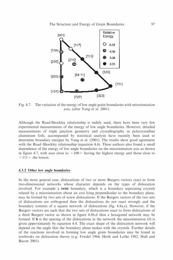
Although the Read-Shockley relationship is widely used, there have been very fewexperimental measurements of the energy of low angle boundaries. However, detailedmeasurements of triple junction geometry and crystallography in polycrystallinealuminium foils, accompanied by statistical analysis have recently been used todetermine boundary energies by Yang et al. (2001). The results show good agreementwith the Read–Shockley relationship (equation 4.6). These authors also found a smalldependence of the energy of low angle boundaries on the misorientation axis as shownin figure 4.7, with axes close to <100> having the highest energy and those close to<111> the lowest.

4.3.2 Other low angle boundaries

In the more general case, dislocations of two or more Burgers vectors react to formtwo-dimensional networks whose character depends on the types of dislocationinvolved. For example a twist boundary, which is a boundary separating crystalsrelated by a misorientation about an axis lying perpendicular to the boundary plane,may be formed by two sets of screw dislocations. If the Burgers vectors of the two setsof dislocations are orthogonal then the dislocations do not react strongly and theboundary consists of a square network of dislocations (fig. 4.8a,c). However, if theBurgers vectors are such that the two sets of dislocations react to form dislocations ofa third Burgers vector as shown in figure 4.8b,d then a hexagonal network may beformed. If h is the spacing of the dislocations in the network the misorientation (�) isgiven approximately by equation 4.4. The exact shape of the dislocation network willdepend on the angle that the boundary plane makes with the crystals. Further detailsof the reactions involved in forming low angle grain boundaries may be found intextbooks on dislocation theory (e.g. Friedel 1964, Hirth and Lothe 1982, Hull andBacon 2001).

Fig. 4.7. The variation of the energy of low angle grain boundaries with misorientationaxis, (after Yang et al. 2001).


4.4 HIGH ANGLE GRAIN BOUNDARIES

Although the structure of low angle grain boundaries is reasonably well understood,much less is known about the structure of high angle grain boundaries. Early theoriessuggested that the grain boundary consisted of a thin ‘amorphous layer’ (§1.2.1), but it isnow known that these boundaries consist of regions of good and bad matching betweenthe two grains. The concept of the coincidence site lattice (CSL) (Kronberg and Wilson1949), and extensive computer modelling, together with atomic resolution microscopyhave in recent years considerably advanced the subject.

4.4.1 The coincidence site lattice

Consider two interpenetrating crystal lattices and translate them so as to bring a latticepoint of each into coincidence, as in figure 4.9. If other points in the two lattices coincide

Fig. 4.8. The formation of low angle twist boundaries from dislocation arrays.(a) A square network formed from screw dislocations of orthogonal Burgers

vector, (b) A hexagonal network formed by screw dislocations with 120� Burgersvectors, (c) TEM micrograph of a square twist boundary in copper, (Humphreysand Martin 1968), (d) TEM micrograph of a hexagonal twist boundary in copper,

(Humphreys and Martin 1968).


(the solid circles in fig. 4.9), then these points form the coincident site lattice.The reciprocal of the ratio of CSL sites to lattice sites is denoted by �. For examplein figure 4.9, � is seen to be 5. In the general case where there is no simpleorientation relationship between the grains, � is large and the boundary, which hasno special properties, is often referred to as a random boundary. However,for certain orientation relationships for which there is a good fit between the grains,� is small and this may confer some special properties on the boundary. Good examplesof this are the coherent twin (�3) boundary shown in figure 4.10, low angle grainboundaries (�1), and the high mobility �7 boundaries in fcc materials which arediscussed in §5.3.2.

Table 4.1

Rotation axes and angles for coincidence site lattices of �<31.

� ��min Axis Frequency %

1 0 Any 2.28

3 60 <111> 1.76

5 36.87 <100> 1.23

7 38.21 <111> 0.99

9 38.94 <110> 1.02

11 50.48 <110> 0.75

13a 22.62 <100> 0.29

13b 27.80 <111> 0.39

15 48.19 <210> 0.94

17a 28.07 <100> 0.20

17b 61.93 <221> 0.39

19a 26.53 <110> 0.33

19b 46.83 <111> 0.22

21a 21.79 <111> 0.19

21b 44.40 <211> 0.57

23 40.45 <311> 0.50

25a 16.25 <100> 0.11

25b 51.68 <331> 0.44

27a 31.58 <110> 0.20

27b 35.42 <210> 0.39

29a 43.61 <100> 0.09

29b 46.39 <221> 0.35

Data from Mykura 1980. Column 4, lists the frequencies of the occurrence of the boundaries

predicted for a random grain assemble (Pan and Adams 1994), using the Brandon criterion.


The concept of Grain Boundary Engineering, in which the properties of the material areimproved by processing the material so as to maximise the number of CSL or ‘special’boundaries has been developed in recent years (Watanabe 1984), and is discussed inmore detail in §11.3.2.3.

Further details of the geometry of CSL boundaries and extensive tables of CSLrelationships may be found in Brandon et al. (1964), Grimmer et al. (1974), Mykura(1980) and Warrington (1980). Table 4.1 shows the relationship between � and theangle/axis rotation for boundaries up to and including �29.

4.4.2 The structure of high angle boundaries

The atomic structure at the grain boundary is determined by relaxation of the atoms,which is dependent on the nature of the atomic bonding forces, and there has been

Fig. 4.9. A coincident site lattice (�5) formed from two simple cubic lattices rotated by36.9o about an <001> axis. Filled circles denote sites common to both lattices.

Fig. 4.10. A coherent twin (�3) boundary.


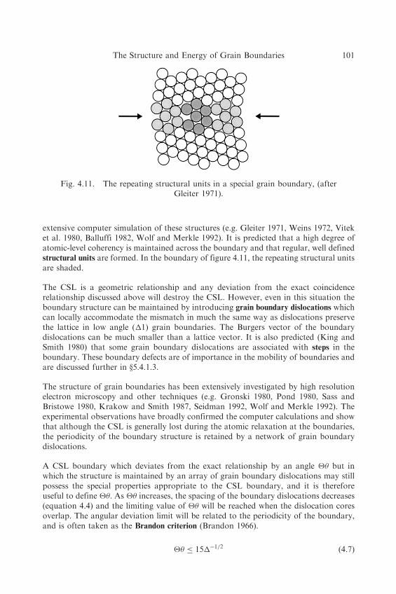
extensive computer simulation of these structures (e.g. Gleiter 1971, Weins 1972, Viteket al. 1980, Balluffi 1982, Wolf and Merkle 1992). It is predicted that a high degree ofatomic-level coherency is maintained across the boundary and that regular, well definedstructural units are formed. In the boundary of figure 4.11, the repeating structural unitsare shaded.

The CSL is a geometric relationship and any deviation from the exact coincidencerelationship discussed above will destroy the CSL. However, even in this situation theboundary structure can be maintained by introducing grain boundary dislocations whichcan locally accommodate the mismatch in much the same way as dislocations preservethe lattice in low angle (�1) grain boundaries. The Burgers vector of the boundarydislocations can be much smaller than a lattice vector. It is also predicted (King andSmith 1980) that some grain boundary dislocations are associated with steps in theboundary. These boundary defects are of importance in the mobility of boundaries andare discussed further in §5.4.1.3.

The structure of grain boundaries has been extensively investigated by high resolutionelectron microscopy and other techniques (e.g. Gronski 1980, Pond 1980, Sass andBristowe 1980, Krakow and Smith 1987, Seidman 1992, Wolf and Merkle 1992). Theexperimental observations have broadly confirmed the computer calculations and showthat although the CSL is generally lost during the atomic relaxation at the boundaries,the periodicity of the boundary structure is retained by a network of grain boundarydislocations.

A CSL boundary which deviates from the exact relationship by an angle �� but inwhich the structure is maintained by an array of grain boundary dislocations may stillpossess the special properties appropriate to the CSL boundary, and it is thereforeuseful to define ��. As �� increases, the spacing of the boundary dislocations decreases(equation 4.4) and the limiting value of �� will be reached when the dislocation coresoverlap. The angular deviation limit will be related to the periodicity of the boundary,and is often taken as the Brandon criterion (Brandon 1966).

�� 15��1=2 ð4:7Þ

Fig. 4.11. The repeating structural units in a special grain boundary, (afterGleiter 1971).


Observations of discrete grain boundary dislocations and measurements of theproperties of special boundaries (see e.g. Palumbo and Aust 1992, Randle 1996)suggest that this criterion is too lax and that a better limit is

�� 15��5=6: ð4:8Þ

4.4.3 The energy of high angle boundaries

On the basis of the structural models outlined above, it might be expected that theenergy of the boundary would be a minimum for an exact coincidence relationshipand that it would increase as the orientation deviated from this, due to the energy ofthe network of accommodating boundary dislocations. However, the correlationbetween the geometry and the energy of a boundary is more complicated than this

Fig. 4.12. The computed (a) and (c) and measured (b) and (d) energies at 650�C forsymmetrical <100> and <110> tilt boundaries in aluminium, (Hasson

and Goux 1971).


(Goodhew 1980) as is illustrated by figure 4.12 which shows a comparison of themeasured and calculated energies of symmetrical tilt boundaries in aluminium. It canbe seen that low energy cusps are found only for the �3 (coherent twin) and �11boundaries and that the predicted cusps for �5 and �9 are not detected. However,more recent measurements of boundary energies in high purity metals (e.g. Miura etal. 1990, Palumbo and Aust 1990) have found evidence for more low energy specialboundaries than were found in earlier work.

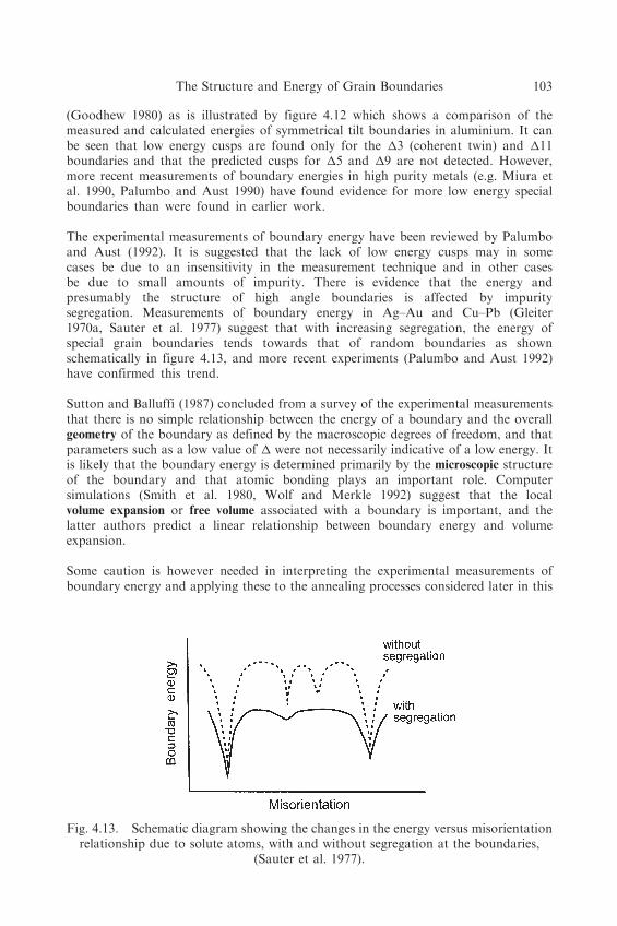
The experimental measurements of boundary energy have been reviewed by Palumboand Aust (1992). It is suggested that the lack of low energy cusps may in somecases be due to an insensitivity in the measurement technique and in other casesbe due to small amounts of impurity. There is evidence that the energy andpresumably the structure of high angle boundaries is affected by impuritysegregation. Measurements of boundary energy in Ag–Au and Cu–Pb (Gleiter1970a, Sauter et al. 1977) suggest that with increasing segregation, the energy ofspecial grain boundaries tends towards that of random boundaries as shownschematically in figure 4.13, and more recent experiments (Palumbo and Aust 1992)have confirmed this trend.

Sutton and Balluffi (1987) concluded from a survey of the experimental measurementsthat there is no simple relationship between the energy of a boundary and the overallgeometry of the boundary as defined by the macroscopic degrees of freedom, and thatparameters such as a low value of � were not necessarily indicative of a low energy. Itis likely that the boundary energy is determined primarily by the microscopic structureof the boundary and that atomic bonding plays an important role. Computersimulations (Smith et al. 1980, Wolf and Merkle 1992) suggest that the localvolume expansion or free volume associated with a boundary is important, and thelatter authors predict a linear relationship between boundary energy and volumeexpansion.

Some caution is however needed in interpreting the experimental measurements ofboundary energy and applying these to the annealing processes considered later in this

Fig. 4.13. Schematic diagram showing the changes in the energy versus misorientationrelationship due to solute atoms, with and without segregation at the boundaries,

(Sauter et al. 1977).


book, because such measurements are normally made at very high homologoustemperatures in order for equilibrium to be achieved. There is evidence bothfrom experiments (Gleiter and Chalmers 1972, Goodhew 1980, Shvindlerman andStraumal 1985, Rabkin et al. 1991, Sutton and Balluffi 1995, Gottstein andShvindlerman 1999), and molecular dynamic simulations (Wolf 2001) that some specialboundaries may exhibit a phase transition at very high temperatures, and that this mayinvolve either a transformation to a different ordered structure or to a liquid-likestructure. Such transitions will have significant effects on the boundary energies and onother properties such as diffusion and mobility, as is further discussed in §5.3.1.

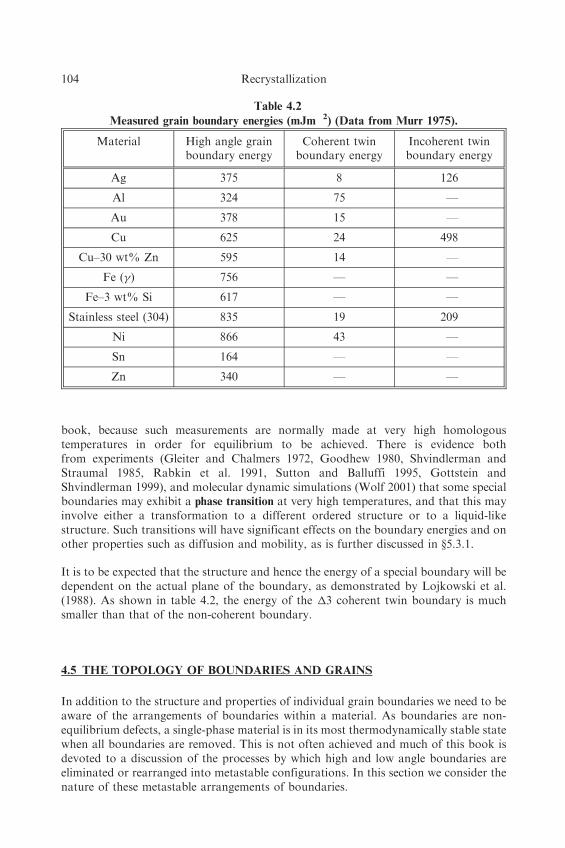
It is to be expected that the structure and hence the energy of a special boundary will bedependent on the actual plane of the boundary, as demonstrated by Lojkowski et al.(1988). As shown in table 4.2, the energy of the �3 coherent twin boundary is muchsmaller than that of the non-coherent boundary.

4.5 THE TOPOLOGY OF BOUNDARIES AND GRAINS

In addition to the structure and properties of individual grain boundaries we need to beaware of the arrangements of boundaries within a material. As boundaries are non-equilibrium defects, a single-phase material is in its most thermodynamically stable statewhen all boundaries are removed. This is not often achieved and much of this book isdevoted to a discussion of the processes by which high and low angle boundaries areeliminated or rearranged into metastable configurations. In this section we consider thenature of these metastable arrangements of boundaries.

Table 4.2

Measured grain boundary energies (mJm�2) (Data from Murr 1975).

Material High angle grainboundary energy

Coherent twinboundary energy

Incoherent twinboundary energy

Ag 375 8 126

Al 324 75 —

Au 378 15 —

Cu 625 24 498

Cu–30 wt% Zn 595 14 —

Fe (�) 756 — —

Fe–3 wt% Si 617 — —

Stainless steel (304) 835 19 209

Ni 866 43 —

Sn 164 — —

Zn 340 — —


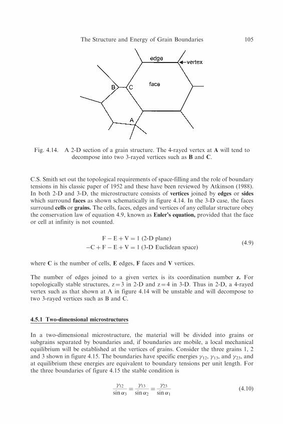
C.S. Smith set out the topological requirements of space-filling and the role of boundarytensions in his classic paper of 1952 and these have been reviewed by Atkinson (1988).In both 2-D and 3-D, the microstructure consists of vertices joined by edges or sides

which surround faces as shown schematically in figure 4.14. In the 3-D case, the facessurround cells or grains. The cells, faces, edges and vertices of any cellular structure obeythe conservation law of equation 4.9, known as Euler’s equation, provided that the faceor cell at infinity is not counted.

F� Eþ V ¼ 1 ð2-D planeÞ

�Cþ F� Eþ V ¼ 1 ð3-D Euclidean spaceÞð4:9Þ

where C is the number of cells, E edges, F faces and V vertices.

The number of edges joined to a given vertex is its coordination number z. Fortopologically stable structures, z¼ 3 in 2-D and z¼ 4 in 3-D. Thus in 2-D, a 4-rayedvertex such as that shown at A in figure 4.14 will be unstable and will decompose totwo 3-rayed vertices such as B and C.

4.5.1 Two-dimensional microstructures

In a two-dimensional microstructure, the material will be divided into grains orsubgrains separated by boundaries and, if boundaries are mobile, a local mechanicalequilibrium will be established at the vertices of grains. Consider the three grains 1, 2and 3 shown in figure 4.15. The boundaries have specific energies �12, �13, and �23, andat equilibrium these energies are equivalent to boundary tensions per unit length. Forthe three boundaries of figure 4.15 the stable condition is

�12sin�3

¼�13

sin�2¼

�23sin �1

ð4:10Þ

Fig. 4.14. A 2-D section of a grain structure. The 4-rayed vertex at A will tend todecompose into two 3-rayed vertices such as B and C.


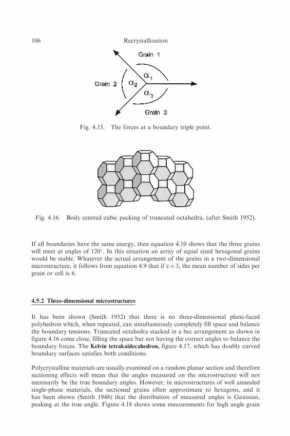
If all boundaries have the same energy, then equation 4.10 shows that the three grainswill meet at angles of 120�. In this situation an array of equal sized hexagonal grainswould be stable. Whatever the actual arrangement of the grains in a two-dimensionalmicrostructure, it follows from equation 4.9 that if z¼ 3, the mean number of sides pergrain or cell is 6.

4.5.2 Three-dimensional microstructures

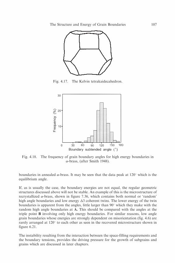
It has been shown (Smith 1952) that there is no three-dimensional plane-facedpolyhedron which, when repeated, can simultaneously completely fill space and balancethe boundary tensions. Truncated octahedra stacked in a bcc arrangement as shown infigure 4.16 come close, filling the space but not having the correct angles to balance theboundary forces. The Kelvin tetrakaidecahedron, figure 4.17, which has doubly curvedboundary surfaces satisfies both conditions.

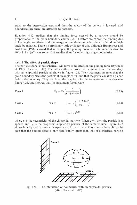
Polycrystalline materials are usually examined on a random planar section and thereforesectioning effects will mean that the angles measured on the microstructure will notnecessarily be the true boundary angles. However, in microstructures of well annealedsingle-phase materials, the sectioned grains often approximate to hexagons, and ithas been shown (Smith 1948) that the distribution of measured angles is Gaussian,peaking at the true angle. Figure 4.18 shows some measurements for high angle grain

Fig. 4.15. The forces at a boundary triple point.

Fig. 4.16. Body centred cubic packing of truncated octahedra, (after Smith 1952).


boundaries in annealed �-brass. It may be seen that the data peak at 120� which is theequilibrium angle.

If, as is usually the case, the boundary energies are not equal, the regular geometricstructures discussed above will not be stable. An example of this is the microstructure ofrecrystallized �-brass, shown in figure 7.36, which contains both normal or ‘random’high angle boundaries and low energy �3 coherent twins. The lower energy of the twinboundaries is apparent from the angles, little larger than 90� which they make with therandom high angle boundaries at A. This should be compared with the angles at thetriple point B involving only high energy boundaries. For similar reasons, low anglegrain boundaries whose energies are strongly dependent on misorientation (fig. 4.6) arerarely arranged at 120� to each other as seen in the recovered microstructure shown infigure 6.21.

The instability resulting from the interaction between the space-filling requirements andthe boundary tensions, provides the driving pressure for the growth of subgrains andgrains which are discussed in later chapters.

Fig. 4.18. The frequency of grain boundary angles for high energy boundaries in�-brass, (after Smith 1948).

Fig. 4.17. The Kelvin tetrakaidecahedron.


4.5.3 Grain boundary facets

The example of �3 twin boundaries discussed above and shown in figure 7.36, is anextreme example of grain boundaries developing facets. Faceting of grain boundarieshas long been known to occur in many metals (see e.g. Sutton and Balluffi 1995,Gottstein and Shvindlerman 1999). In order for a boundary to be facettedspontaneously, the decrease in the total boundary energy must overcome the increasein the total boundary area. Faceting is therefore only likely to occur under conditionswhen the boundary energy depends strongly on the boundary plane, and the mostcommon situation is for low energy CSL boundaries. It is found that the facetingbehaviour of a particular boundary may be strongly dependent on the impurity level(Ference and Balluffi 1988), and on the temperature (Hsieh and Balluffi 1989). Figure4.19 shows the effect of boundary inclination angle on the relative energies ofasymmetric �11 {110] boundaries in copper (Goukon et al. 2000) and this has beenfound to correlate well with the faceting behaviour. Faceting of the boundaries ofrecrystallizing grains is also sometimes observed (§5.3.2.2), and an example is seen infigure 5.16.

4.5.4 Boundary connectivity

The importance of non-random distribution of grain orientations or texture iswidely recognised and discussed in detail in chapters 3 and 12. However, it hasalso been suggested that the non-random spatial distribution of grain misorientations

may also be important, particularly for CSL boundaries. If such boundaries havevalues of properties such as strength or diffusivity which are markedly different from theother boundaries, then clustering effects and their linking or connectivity may have aninfluence on the chemical, physical or mechanical properties of the material (Watanabe1994), and such effects are an important consideration in grain boundary engineering

(§11.3.2.3).

Fig. 4.19. The relative boundary energy for asymmetric [110] �11 tilt boundaries incopper, as a function of boundary inclination, (after Goukon et al. 2000).


4.5.5 Triple junctions

Although in this chapter we are mainly concerned with the properties of the grain facesor boundaries, there is evidence that the properties of the vertices or triple junctions mayplay a role in microstructural evolution and have an influence on grain growth and thisis considered in §5.5.

4.6 THE INTERACTION OF SECOND-PHASE PARTICLES

WITH BOUNDARIES

A dispersion of particles will exert a retarding force or pressure on a low angle or highangle grain boundary and this may have a profound effect on the processes of recovery,recrystallization and grain growth. The effect is known as Zener drag after the originalanalysis by Zener which was published by Smith (1948). The magnitude of thisinteraction depends the nature of the particle and interface, and the shape, size, spacingand volume fraction of the particles. The definitions of the parameters of a second phasedistribution are given in appendix 2.8.

4.6.1 The drag force exerted by a single particle

4.6.1.1 General considerations

Let us consider first, the interaction of a boundary of specific energy � with a sphericalparticle of radius r which has an incoherent interface.

If the boundary meets the particle at an angle � as shown in figure 4.20 then therestraining force on the boundary is:

F ¼ 2�r� cos� sin� ð4:11Þ

The maximum restraining effect (FS) is obtained when �¼ 45�, when

FS ¼ �r� ð4:12Þ

As discussed by Nes et al. (1985), there have been many different derivations of thisforce, but the result is usually similar to the above. It should be noted that when aboundary intersects a particle, the particle effectively removes a region of boundary

Fig. 4.20. The interaction between a grain boundary and a spherical particle.


equal to the intersection area and thus the energy of the system is lowered, andboundaries are therefore attracted to particles.

Equation 4.12 predicts that the pinning force exerted by a particle should beproportional to the grain boundary energy (�). Therefore we expect the pinning dueto low angle boundaries and low energy � boundaries to be less than for ‘random’ highangle boundaries. There is surprisingly little evidence of this, although Humphreys andArdakani (1996) showed that in copper, the pinning pressure on boundaries close to40�<111> (�7) was some 10% smaller than for other high angle boundaries.

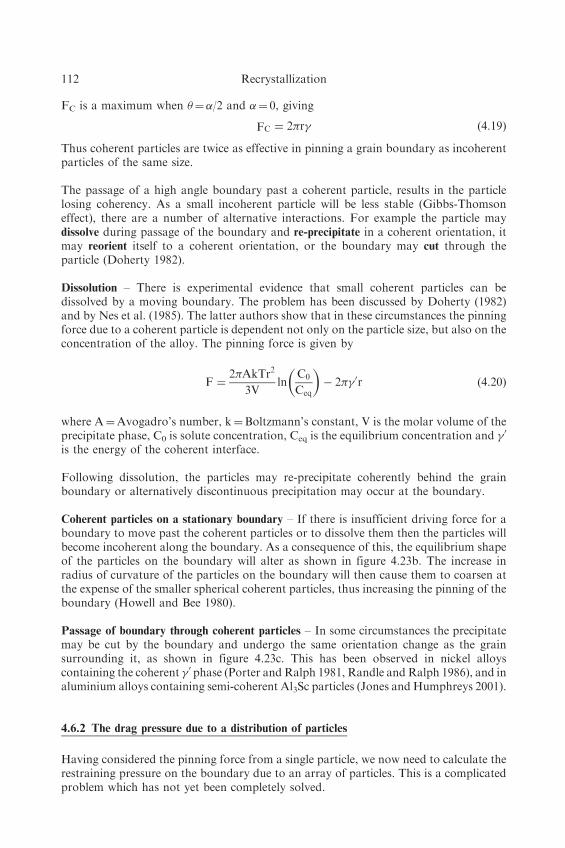
4.6.1.2 The effect of particle shape

The particle shape, if not spherical, will have some effect on the pinning force (Ryum etal. 1983, Nes et al. 1985). The latter authors considered the interaction of a boundarywith an ellipsoidal particle as shown in figure 4.21. Their treatment assumes that thegrain boundary meets the particle at an angle of 90� and that the particle makes a planarhole in the boundary. They calculated the drag force for the two extreme cases shown infigure 4.21, and showed that the maximum forces were

Case 1 F1 ¼ FS2

ð1þ eÞ e1=3

� �ð4:13Þ

Case 2 for e � 1 F2 ¼ FS1þ 2:14e

� e1=2

� �ð4:14Þ

Case 2 for e � 1 F2 ¼ FS e0:47 ð4:15Þ

where e is the eccentricity of the ellipsoidal particle. When e¼ 1 then the particle is asphere, and FS is the drag from a spherical particle of the same volume. Figure 4.22shows how F1 and F2 vary with aspect ratio for a particle of constant volume. It can beseen that the pinning force is only significantly larger than that of a spherical particle

Fig. 4.21. The interaction of boundaries with an ellipsoidal particle,(after Nes et al. 1985).


for the case of thin plates meeting the boundary face-on and long needles meetingthe boundary edge-on.

Ringer et al. (1989) have analysed the interaction of a boundary with cubic particles.The strength of the interaction depends upon the orientation of the cube relative to theboundary and in the extreme case, when the cube side is parallel to the boundary, thedrag force is almost twice that of a sphere of the same volume. However, as this is aspecial case, it is unlikely to be a very significant factor in practice.

4.6.1.3 Coherent particles

If a high angle grain boundary moves past a coherent particle then the particle willgenerally lose coherence during the passage of the boundary. As the energy of theincoherent interface is greater than that of the original coherent interface, energy isrequired to cause this transformation, and this energy must be supplied by the movingboundary. Therefore, as first shown by Ashby et al. (1969), coherent particles will bemore effective in pinning boundaries than will incoherent particles.

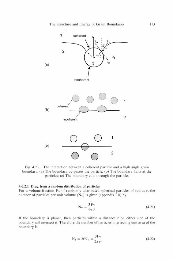
Following the analysis by Nes et al. (1985), if the grains are denoted 1 and 2 and theparticle as 3, as in figure 4.23a, then there are now three different boundary energies �12,�13 and �23. These boundaries meet at the particle surface, and if equilibrium isestablished then

�23 ¼ �31 þ �12 cos � ð4:16Þ

and

cos� ¼�23� �13

�12ð4:17Þ

The drag force is then

FC ¼ 2�r� cosð�� Þ cos� ð4:18Þ

Fig. 4.22. The drag force as a function of particle aspect ratio for the two casesillustrated in figure 4.21, (after Nes et al. 1985).


FC is a maximum when �¼ �/2 and �¼ 0, giving

FC ¼ 2�r� ð4:19Þ

Thus coherent particles are twice as effective in pinning a grain boundary as incoherentparticles of the same size.

The passage of a high angle boundary past a coherent particle, results in the particlelosing coherency. As a small incoherent particle will be less stable (Gibbs-Thomsoneffect), there are a number of alternative interactions. For example the particle maydissolve during passage of the boundary and re-precipitate in a coherent orientation, itmay reorient itself to a coherent orientation, or the boundary may cut through theparticle (Doherty 1982).

Dissolution – There is experimental evidence that small coherent particles can bedissolved by a moving boundary. The problem has been discussed by Doherty (1982)and by Nes et al. (1985). The latter authors show that in these circumstances the pinningforce due to a coherent particle is dependent not only on the particle size, but also on theconcentration of the alloy. The pinning force is given by

F ¼2�AkTr2

3Vln

C0

Ceq

� �� 2�� 0r ð4:20Þ

where A¼Avogadro’s number, k¼Boltzmann’s constant, V is the molar volume of theprecipitate phase, C0 is solute concentration, Ceq is the equilibrium concentration and � 0

is the energy of the coherent interface.

Following dissolution, the particles may re-precipitate coherently behind the grainboundary or alternatively discontinuous precipitation may occur at the boundary.

Coherent particles on a stationary boundary – If there is insufficient driving force for aboundary to move past the coherent particles or to dissolve them then the particles willbecome incoherent along the boundary. As a consequence of this, the equilibrium shapeof the particles on the boundary will alter as shown in figure 4.23b. The increase inradius of curvature of the particles on the boundary will then cause them to coarsen atthe expense of the smaller spherical coherent particles, thus increasing the pinning of theboundary (Howell and Bee 1980).

Passage of boundary through coherent particles – In some circumstances the precipitatemay be cut by the boundary and undergo the same orientation change as the grainsurrounding it, as shown in figure 4.23c. This has been observed in nickel alloyscontaining the coherent � 0 phase (Porter andRalph 1981, Randle andRalph 1986), and inaluminium alloys containing semi-coherent Al3Sc particles (Jones and Humphreys 2001).

4.6.2 The drag pressure due to a distribution of particles

Having considered the pinning force from a single particle, we now need to calculate therestraining pressure on the boundary due to an array of particles. This is a complicatedproblem which has not yet been completely solved.


4.6.2.1 Drag from a random distribution of particles

For a volume fraction FV of randomly distributed spherical particles of radius r, thenumber of particles per unit volume (NV) is given (appendix 2.8) by

NV ¼3FV

4� r3ð4:21Þ

If the boundary is planar, then particles within a distance r on either side of theboundary will intersect it. Therefore the number of particles intersecting unit area of theboundary is

NS ¼ 2rNV ¼3FV

2� r2ð4:22Þ

Fig. 4.23. The interaction between a coherent particle and a high angle grainboundary. (a) The boundary by-passes the particle; (b) The boundary halts at the

particles; (c) The boundary cuts through the particle.


The pinning pressure exerted by the particles on unit area of the boundary is given by

PZ ¼ NSFS ð4:23Þ

and hence from equations 4.12 and 4.22

PZ ¼3FV�

2rð4:24Þ

This type of relationship was first proposed by Zener (Smith 1948), although in theoriginal paper because NS was taken as r. NV, the pinning pressure was half that ofequation 4.21. PZ as given by equation 4.24 is commonly known as the Zener pinning

pressure.

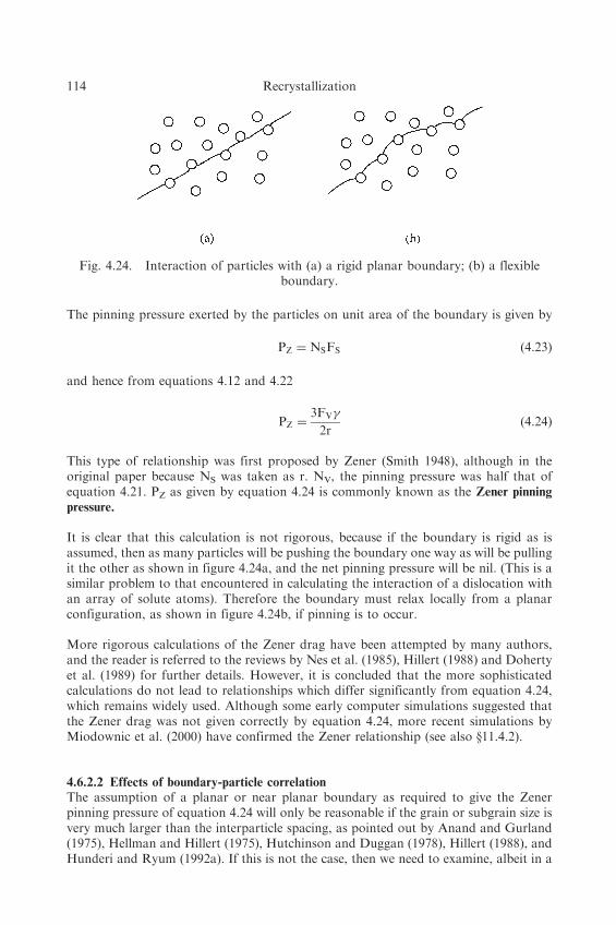
It is clear that this calculation is not rigorous, because if the boundary is rigid as isassumed, then as many particles will be pushing the boundary one way as will be pullingit the other as shown in figure 4.24a, and the net pinning pressure will be nil. (This is asimilar problem to that encountered in calculating the interaction of a dislocation withan array of solute atoms). Therefore the boundary must relax locally from a planarconfiguration, as shown in figure 4.24b, if pinning is to occur.

More rigorous calculations of the Zener drag have been attempted by many authors,and the reader is referred to the reviews by Nes et al. (1985), Hillert (1988) and Dohertyet al. (1989) for further details. However, it is concluded that the more sophisticatedcalculations do not lead to relationships which differ significantly from equation 4.24,which remains widely used. Although some early computer simulations suggested thatthe Zener drag was not given correctly by equation 4.24, more recent simulations byMiodownic et al. (2000) have confirmed the Zener relationship (see also §11.4.2).

4.6.2.2 Effects of boundary-particle correlation

The assumption of a planar or near planar boundary as required to give the Zenerpinning pressure of equation 4.24 will only be reasonable if the grain or subgrain size isvery much larger than the interparticle spacing, as pointed out by Anand and Gurland(1975), Hellman and Hillert (1975), Hutchinson and Duggan (1978), Hillert (1988), andHunderi and Ryum (1992a). If this is not the case, then we need to examine, albeit in a

Fig. 4.24. Interaction of particles with (a) a rigid planar boundary; (b) a flexibleboundary.


simplified way, the consequences. In figure 4.25 we identify four important cases. Infigure 4.25a the grains are much smaller than the particle spacing, in figure 4.25b theparticle spacing and grain size are similar, in figure 4.25c the grain size is much largerthan the particle spacing and in figure 4.25d, the particles are inhomogeneouslydistributed so as to lie only on the boundaries. In all these cases there is a strongcorrelation between the particles and the boundaries, although an accurate assessmentof the pinning force is difficult and is dependent on the details of the particle and grain(or subgrain) arrangement.

Consider the particles and boundaries which form the three-dimensional cubic arraysshown in figure 4.25. For case a, it is reasonable to assume that all the particles lie notonly on boundaries, but at vertices in the grain structure, because in these positions theparticles, by removing the maximum boundary area, minimise the energy of the system.

If the grain edge length is D, then the grain boundary area per unit volume is 3/D. Thenumber of particles per unit area of boundary (NA) is given by

NA ¼�NVD

3ð4:25Þ

where � is a factor which depends on the positions of the particles in the boundaries. Forparticles on boundary faces, �¼ 1. For particles at the vertices as shown in figures 4.25

Fig. 4.25. Schematic diagram of the correlation between particles and boundaries as afunction of grain size.


(a) and (b), �¼ 3 and hence, using equation 4.21

NA ¼�NVD

3¼

3DFV

4� r3ð4:26Þ

For incoherent spherical particles the pinning pressure on the boundary (P0Z) will thenbe given by

P0Z ¼ FSNA ¼3DFV�

4 r2ð4:27Þ

This relationship will be valid for grain sizes up to and including that shown in figure4.25b, in which the grain size and particle spacing are the same (DC). In this situation,the spacing of the particles on the cubic lattice (L) is equal to DC and is given by

L ¼ DC ¼ N�1=3V ¼4� r3

3FV

� �1=3

ð4:28Þ

at which point the pinning force reaches a maximum P0Zmax given by

P0Zmax �1:2� F

2=3V

rð4:29Þ

As the grain size increases beyond DC, the number of particles per unit area of boundary(NA) will decrease from that given by equation 4.26 and eventually reach NS as given byequation 4.22. We can treat this transition from correlated to non-correlated boundaryin the following approximate manner.

The number of boundary corners per unit volume in a material of grain size D is givenapproximately by 1/D3, and the fraction of particles lying on these potent pinning sitesis therefore, for the condition D�DC.

X ¼1

NV D3ð4:30Þ

When D¼DC then from equation 4.28 we find X¼ 1. Thus as the grains grow, adiminishing fraction of particles is able to sit at the grain corners.

The number of corner-sited particles per unit area of boundary is then

NC ¼ XNVD ð4:31Þ

The remaining particles will sit on grain boundaries or grain edges or lie within thegrains. In this simple analysis we assume that the particles which are not sitting atgrain corners are intersected at random by boundaries and therefore the number perunit area is

Nr ¼ 2rNVð1�XÞ ð4:32Þ


Thus the total number of particles per unit area of boundary is NcþNr and, usingequation 4.23, the pinning pressure is given by

P00Z ¼ �r�½XNV Dþ ð1�XÞ2NV r� ð4:33Þ

or, when D�DC

P00Z ¼ �r�1

D2þ ð1�

1

NV D3Þ2NV r

� �ð4:34Þ

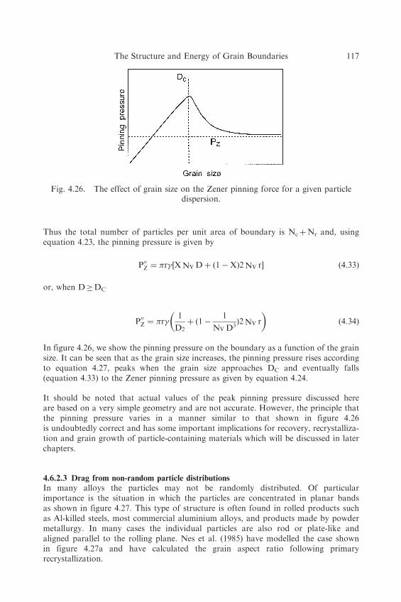
In figure 4.26, we show the pinning pressure on the boundary as a function of the grainsize. It can be seen that as the grain size increases, the pinning pressure rises accordingto equation 4.27, peaks when the grain size approaches DC and eventually falls(equation 4.33) to the Zener pinning pressure as given by equation 4.24.

It should be noted that actual values of the peak pinning pressure discussed hereare based on a very simple geometry and are not accurate. However, the principle thatthe pinning pressure varies in a manner similar to that shown in figure 4.26is undoubtedly correct and has some important implications for recovery, recrystalliza-tion and grain growth of particle-containing materials which will be discussed in laterchapters.

4.6.2.3 Drag from non-random particle distributions

In many alloys the particles may not be randomly distributed. Of particularimportance is the situation in which the particles are concentrated in planar bandsas shown in figure 4.27. This type of structure is often found in rolled products suchas Al-killed steels, most commercial aluminium alloys, and products made by powdermetallurgy. In many cases the individual particles are also rod or plate-like andaligned parallel to the rolling plane. Nes et al. (1985) have modelled the case shownin figure 4.27a and have calculated the grain aspect ratio following primaryrecrystallization.

Fig. 4.26. The effect of grain size on the Zener pinning force for a given particledispersion.


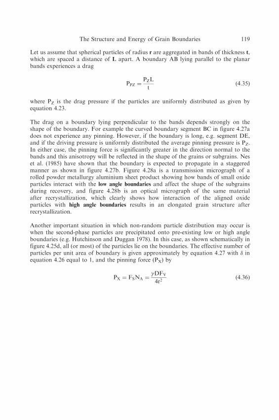
Fig. 4.28. (a) Transmission electron micrograph illustrating the pinning of low angleboundaries by planar arrays of small oxide particles in a rolled aluminium billet

produced by powder metallurgy, (TD plane sections); (b) Optical micrograph of thesame material after recrystallization showing an elongated grain structure,

(Bowen et al. 1993).

Fig. 4.27. The interaction of boundaries with planar arrays of particles. (a) The effectof boundary orientation on pinning; (b) Propagation of a boundary through planar

arrays of particles, (after Nes et al. 1985).


Let us assume that spherical particles of radius r are aggregated in bands of thickness t,which are spaced a distance of L apart. A boundary AB lying parallel to the planarbands experiences a drag

PPZ ¼PZL

tð4:35Þ

where PZ is the drag pressure if the particles are uniformly distributed as given byequation 4.23.

The drag on a boundary lying perpendicular to the bands depends strongly on theshape of the boundary. For example the curved boundary segment BC in figure 4.27adoes not experience any pinning. However, if the boundary is long, e.g. segment DE,and if the driving pressure is uniformly distributed the average pinning pressure is PZ.In either case, the pinning force is significantly greater in the direction normal to thebands and this anisotropy will be reflected in the shape of the grains or subgrains. Neset al. (1985) have shown that the boundary is expected to propagate in a staggeredmanner as shown in figure 4.27b. Figure 4.28a is a transmission micrograph of arolled powder metallurgy aluminium sheet product showing how bands of small oxideparticles interact with the low angle boundaries and affect the shape of the subgrainsduring recovery, and figure 4.28b is an optical micrograph of the same materialafter recrystallization, which clearly shows how interaction of the aligned oxideparticles with high angle boundaries results in an elongated grain structure afterrecrystallization.

Another important situation in which non-random particle distribution may occur iswhen the second-phase particles are precipitated onto pre-existing low or high angleboundaries (e.g. Hutchinson and Duggan 1978). In this case, as shown schematically infigure 4.25d, all (or most) of the particles lie on the boundaries. The effective number ofparticles per unit area of boundary is given approximately by equation 4.27 with � inequation 4.26 equal to 1, and the pinning force (PX) by

PX ¼ FSNA ¼�DFV

4r2ð4:36Þ


Documents

Chapter 4 THE STRUCTURE AND ENERGY OF GRAIN BOUNDARIESusers.encs.concordia.ca/~mmedraj/tmg-books... · 2007-08-14 · Chapter 4 THE STRUCTURE AND ENERGY OF GRAIN BOUNDARIES 4.1 INTRODUCTION