CHAPTER 4 Steam power plants - WIT Press · CHAPTER 4 Steam power plants E. Khalil Department of Mechanical Power Engineering, Cairo University, Cairo, Egypt. Abstract The efﬁ cient

CHAPTER 4

Steam power plants

E. KhalilDepartment of Mechanical Power Engineering, Cairo University, Cairo, Egypt.

Abstract

The effi cient utilization of fossil energy in power generation together with low pollution in conventional thermal power plants is a topic that is gaining interest internationally. The energy availability and sustainability scenario is an area of growing interest and demand in many countries worldwide due to the greater desire to enhance standards of living, increase productivity and preserve a clean environment. Effi cient energy use is favorable for better productivity, product quality, costs, and quality of human life but the use of energy adversely impacts our envi-ronment. The fundamental concepts of power generation had been refi ned to enhance the power generation effi ciency through the use of modern techniques of waste heat recovery and co-generation. This chapter summarizes the basic power cycles in steam power plants and outlines the various methods of improvement. The main goal of effi cient power generation is, among others, to rationalize the use of fossil fuels and enhance the combustion effi ciencies. This is outlined in this chapter through a review of the various combustion modeling techniques for furnace fl ames under steady and time dependent confi gurations. The ability of numerical computations to predict the boiler furnace thermal behavior is an ultimate goal. The heat transfer to furnace walls through thermal radiation is reviewed briefl y to demonstrate the present capabilities. Boiler furnace walls are subject to the major problems of fouling that result in deterioration of the per-formance and drastic reduction of the heat transfer characteristics. This work briefl y highlights the fouling problem in power plant water walls and proposes a monitoring, inspection, and maintenance schedule. The information provides a quick guide on the commonly faced operation problems and methods to enhance energy conversion effi ciency.

www.witpress.com, ISSN 1755-8336 (on-line) WIT Transactions on State of the Art in Science and Engineering, Vol , © 20 WIT Press42 08

doi:10.2495/978-1-84564- - /062 0 04

100 Thermal Engineering in Power Systems

1 Introduction

Centralized power generation became possible when it was recognized that alternating current power lines can transport electricity at low costs across great distances by taking advantage of the ability to raise and lower the voltage using power transformers. Since 1881, electricity has been generated for the purpose of powering human technologies from various sources of energy. The fi rst power plants were run on water power or coal, and today we rely mainly on coal, nuclear, natural gas, hydroelectric, and petroleum with a small amount from solar energy, tidal harnesses, wind generators, and geothermal sources. Rotating turbines attached to electrical generators produce most commercially available electricity. Turbines are driven by a fl uid, which acts as an intermediate energy carrier. The fl uids typically used are:

Steam in steam turbines• – Water is boiled by nuclear fi ssion or the burning of fossil fuels (coal, natural gas, or petroleum). Some newer plants use the sun as the heat source: solar parabolic troughs and solar power towers concentrate sunlight to heat a heat transfer fl uid, which is then used to produce steam. Another renewable source of heat used to drive a turbine is geothermal power. Either steam under pressure emerges from the ground and drives a turbine or hot water evaporates a low-boiling liquid to create vapor to drive a turbine.Water in hydraulic turbines• – Turbine blades are acted upon by fl owing water, produced by hydroelectric dams or tidal forces.Wind• – Most wind turbines generate electricity from naturally occurring wind. Solar updraft towers use wind that is artifi cially produced inside the chimney by heating it with sunlight.Hot gases in gas turbines• – Turbines are driven directly by gases produced by the combustion of natural gas or oil.

Combined cycle gas turbine plants are driven by both steam and gas. They generate power by burning natural gas in a gas turbine and use residual heat to generate additional electricity from steam. These plants offer effi ciencies of up to 60%.

Various other technologies have been studied and developed for power generation. Solid-state generation (without moving parts) is of particular interest in portable applications. This area is largely dominated by thermoelectric (TE) devices, though thermionic (TI) and thermo-photovoltaic (TPV) systems have been developed as well. Typically, TE devices are used at lower temperatures than TI and TPV systems. Piezoelectric devices are used for power generation from mechanical strain, particularly in power harvesting. Betavoltaics are another type of solid-state power generator, which produces electricity from radioactive decay. Fluid-based magnetohydrodynamic power generation has been studied as a method for extract-ing electrical power from nuclear reactors and also from more conventional fuel combustion systems. Electrochemical electricity generation is also important in portable and mobile applications. Currently, most electrochemical power comes from closed electrochemical cells (“batteries”), which are arguably utilized more


Steam Power Plants 101

as storage systems than generation systems, but open electrochemical systems, known as fuel cells, have been undergoing a great deal of research and develop-ment in the last few years. Fuel cells can be used to extract power either from natural fuels or from synthesized fuels (mainly electrolytic hydrogen) and so can be viewed as either generation systems or storage systems depending on their use.

Factors and parameters affecting the selection of steam power plant capacities and sites [1]:

1. Types of service (base load or peak load).2. Location (relative to water and fuel).3. Space available (each power plant has a certain area/unit energy produced).4. Reliability: Steam turbine life is extremely long. There are steam turbines that

have been in service for over 50 years. Overhaul intervals are measured in years. When properly operated and maintained (including proper control of boiler water chemistry), steam turbines are extremely reliable. They require controlled thermal transients as the massive casing heats up slowly and differ-ential expansion of the parts must be minimized.

5. Environment: Emissions associated with a steam turbine are dependent on the source of the steam. Steam turbines can be used with a boiler fi ring any one or a combination of a large variety of fuel sources, or they can be used with a gas turbine in a combined cycle confi guration. Boiler emissions vary depending on fuel type and environmental conditions. Boiler emissions include nitrogen oxide (NOx), sulfur oxides (SOx), particulate matter (PM), carbon monoxide (CO), and carbon dioxide (CO2). Recently, NOx control has been the primary focus of emission control research and development in boilers. The following provides a description of the most prominent emission control approaches [2]. Combustion control techniques are less costly than post-combustion control methods and are often used on industrial boilers for NOx control. Control of combustion temperature has been the principal focus of combustion process control in boilers. Combustion control requires tradeoffs – high temperatures favor complete burn-up of the fuel and low residual hydrocarbons and CO, but promote NOx formation. Very lean combustion dilutes the combustion process and reduces combustion temperatures and NOx formation. However, if the mixture is too lean, incomplete combustion occurs, increasing CO emissions [3].

6. Cost (capital cost and maintenance cost): There is broad consensus among scientists that we are not close to running out of fossil fuels. Despite this abun-dance, political considerations over the security of supplies, environmental concerns related to global warming and sustainability might move the world’s energy consumption away from fossil fuels. A government-led move away from fossil fuels would most likely create economic pressure through carbon emissions trading and green taxation. Some countries are taking action as a result of the Kyoto Protocol, and further steps in this direction are proposed. For example, the European Commission has proposed that the energy policy of the European Union should set a binding target of increasing the level of renewable energy in the EU’s overall mix from <7% today to 20% by 2020.



2 Energy scenarios

2.1 Crude oil production

World crude oil production during August 2005 was 74 million barrels per day, up 0.2 million barrels per day from the level in the previous month. OPEC (Organization of the Petroleum Exporting Countries) production during August 2005 averaged 31 million barrels per day, down 0.1 million barrels per day from the level in the previous month. During August 2005, production increased in the United Arab Emirates by 50,000 barrels per day; Algeria by 20,000 barrels per day; Libya by 15,000 barrels per day; and Iran by 10,000 barrels per day. Production decreased in Nigeria and Iraq each by 100,000 barrels per day and remained unchanged in Saudi Arabia, Venezuela, Kuwait, Indonesia, and Qatar. Among the non-OPEC nations, production during August 2005 increased in Mexico by 332,000 barrels per day; Russia by 150,000 barrels per day; the United States by 29,000 barrels per day; and China by 14,000 barrels per day. Production decreased in the United Kingdom by 215,000 barrels per day; Canada by 92,000 barrels per day; Norway by 72,000 barrels per day; and Egypt by 3000 barrels per day [4].

2.2 Petroleum consumption

In July 2005, consumption in all OECD (Organization for Economic Coopera-tion and Development) countries was 49 million barrels per day, 1% (percentage changes are based on unrounded data) lower than the July 2004 rate. Comparing July rates in 2005 and 2004, consumption was higher in 2005 in Canada (+1%) and South Korea (<+1%). The July 2005 consumption rate was lower in Italy (–7%); Germany (–4%); France and Japan (each –2%); the United Kingdom (–1%); and the United States (less than –1%), compared with the rate one year earlier.

2.3 Petroleum stocks

For all OECD countries, petroleum stocks at the end of July 2005 totaled 4.2 billion barrels, 4% (percentage changes are based on unrounded data) higher than the ending stock level in July 2004. Stock levels were higher in July 2005 in the United States (+6%); France (+4%); Germany (+3%); and Canada and Japan (each +2%). Stock levels were lower in the United Kingdom (–6%) and South Korea and Italy (each –2%), compared with levels one year earlier.

3 Steam power plants cycles

3.1 Basic cycle description

Rankine cycles describe the operation of steam heat engines commonly found in power generation plants as schematically shown here in Fig. 1. In such vapor



power plants, power is generated by alternately vaporizing and condensing a working fl uid (in many cases water, although refrigerants such as ammonia may also be used) [1].

There are four processes in the Rankine cycle, each changing the state of the working fl uid. These states are identifi ed by number in Fig. 1.

Process 1-2• s: First, the working fl uid is pumped (ideally isentropically) from low to high pressure by a pump. Pumping requires a power input (for example mechanical or electrical).Process 2• s-3: The high pressure liquid enters a boiler where it is heated at con-stant pressure by an external heat source to become a saturated vapor. Common heat sources for power plant systems are coal, natural gas, or nuclear power.Process 3-4• s: The saturated vapor expands through a turbine to generate power output. Ideally, this expansion is isentropic. This decreases the temperature and pressure of the vapor.Process 4• s-1: The vapor then enters a condenser where it is cooled to become a saturated liquid. This liquid then re-enters the pump and the cycle repeats.

3.2 Actual Rankine cycle

In actual situations, both the water pumps and the steam Turbines do not operate isen-tropically and losses result in more power demand for pumping and less power actu-ally generated by steam to blades [1]. The actual Rankine cycle is shown in Fig. 2.

Such losses are clearly shown in the following comparisons. That is,

h3 – h4 < h3 – h4s and h2 – h1 > h2s – h1

The performance of an actual turbine or pump is usually expressed in terms of isentropic effi ciency. The isentropic effi ciency of a turbine (ηT) is defi ned as the ratio of “work delivered by the actual turbine” to “work delivered by an isentropic turbine.”

Figure 1: Simple Rankine cycle.



h−−

3 4T

3 4s

=h h

h h (1)

The isentropic effi ciency of a pump (ηP) is defi ned as the ratio of “work required by an isentropic pump” to “work required by the actual pump.”

h−−

2s 1P

2 1

=h h

h h (2)

3.3 Effi ciency improvements in power plants

It is well known that the cycle effi ciency is generally proportional to

h −∝ L

H1

TT (3)

The question that emerges is how to improve the cycle effi ciency; naturally through lowering the heat sink temperature TL and/or raising the heat source temperature TH.

3.3.1 Lowering the condenser pressureSetting the steam condenser pressure is generally restricted by the temperature of the available condenser water (lake, river, etc.) typically around 25°C or condenser saturation pressure of around Psat =~3.2 kPa.

Figure 2: Practical Rankine cycle.



The pressure at the exit of the turbine can be less than atmospheric pressure with a condenser and the closed loop of the condenser permits the use of high water quality on the steam cycle side. However, lowering condenser pressure is not unlimited as it depends on the design condenser temperature and the limits of lower steam quality at turbine exit. In Fig. 3, the shaded area represents the gain in network of the system due to lowering the condenser pressure.

3.3.2 Superheating the steam to high temperaturesThe average temperature at which heat is supplied in the boiler can be increased by superheating the steam. Dry saturated steam from the boiler is passed through a second bank of smaller bore tubes within the boiler until the steam reaches the required temperature. The value of TH, the mean temperature at which heat is added, increases, while TL remains constant. Therefore, the effi ciency increases.

The quality of the turbine exhaust termed, x, increases, the value of steam dryness fraction at turbine exit should not be lower than about 0.9 to prevent water droplets effects on blading effi ciency, as outlined in Fig. 4. With suffi cient superheating, the turbine exhaust conditions may well fall in the superheated region.

3.3.3 Increasing the boiler pressureIncreasing the operating pressure of the boiler automatically raises the tempera-ture at which boiling takes place. This consequently raises the average temperature

Figure 3: Lowering condenser temperature TL through decreasing condenser operating pressure [1].



at which heat is added to the steam and thus raises the thermal effi ciency of the cycle as indicated in Fig. 5.An increase in boiler pressure results in a higher TH for the same TL, therefore higher cycle thermal effi ciency η. But state 4′ indicates a lower steam quality than state 4, then more wet steam at the turbine exhaust is expected; this may result in cavitation of the turbine blades at the last low pressure stages. Con-sequently, the effi ciency is decreased and the cost of maintenance increases. It is recommended to keep the steam quality higher than 90% at the turbine exhaust section.

3.3.4 Rankine cycle with reheat

1. The moisture content at the exhaust of the turbine should be no greater than 10% – this can result in physical erosion of the turbine blades.

Figure 4: Increase TH by adding superheat.

Figure 5: Effect of increasing the boiler pressure.



2. As higher boiler pressures are required for high effi ciency, this leads to a higher moisture content ratio in the low pressure turbine expansion [1].

3. To improve the turbine exhaust steam conditions, the steam can be reheated between two turbine expansion stages or steps as indicated in Fig. 6. The follow-ing points emerge:

The temperature of the steam entering the turbine is limited by metallurgical • constraints.Modern boilers can handle up to 30 MPa and a maximum temperature of • tmax ≈ 650°C.Materials, such as ceramic blades, can handle temperatures up to 750°C.•

Advantages of using Rankine cycle with reheat: This arrangement provides high steam quality or even slightly superheated vapor at turbine exit. Therefore, for a given TH the Rankine cycle, effi ciency increases without reducing the steam quality at turbine exit.

Rankine cycle with regeneration: To increase the cycle effi ciency, to near the Carnot cycle effi ciency, added heat QH should be at as high temperature TH as it possibly can. Also, heat should be rejected, QL, at the lowest possible TL. In such confi guration, the Rankine cycle is provided with feed water heaters (FWHs) to heat the high-pressure sub-cooled water at the exit of the pump to the saturation temperature. As shown in Fig. 7, most of the heat addition (QH) is performed at high temperature.

Feed water heaters: There are two different types of FWHs commonly used in power plants: open FWH, where the two streams of high temperature steam and low temperature water mix in an open heater at constant pressure; closed FWH, where a heat exchanger is used to transfer heat between the two streams but the two streams do not mix. The two streams can be naturally maintained at different pressures.

Figure 6: Rankine cycle with reheat.



1. Open FWH: In this arrangement, the working fl uid passes isentropically through the turbine stages and pumps. Steam enters the fi rst stage turbine at state 1 and expands to state 2 – where a fraction of the total fl ow is bled off into an open FWH at P2. The rest of the steam expands into the second stage turbine at state point 3. – This portion of the fl uid is condensed and pumped as a saturated liquid to the FWH at P2. A single mixed stream exits the FWH at state point 6. The mass fl ow rates through each of the components are typically calculated by performing a mass balance over the turbine. A heat balance is also performed to calculate the various enthalpies at various states.

2. Closed FWH: Such confi guration can be practically realized in two alternatives typically:

Pump the condensate back to the high-pressure line (Fig. 8a).• A steam trap is inserted in the condensed steam line that allows only liquid • to pass (Fig. 8b).

The incoming feed water does not mix with the extracted steam; both streams fl ow separately through the heater, hence the two streams can have different pressures.

Advantages of using heat regeneration:

1. It improves the cycle effi ciency.2. It provides a convenient means of deaerating the feed water (removing the air

that leaks in at the condenser) to prevent corrosion in the boiler.3. It also helps to control the large volume fl ow rate of the steam at the fi nal stages

of the turbine.

Figure 9 shows the effect of the number of FWHs on the thermal effi ciency; increas-ing the number of FWHs improves the thermal effi ciency. This is, however, limited by the cost and there is an optimum. Modem steam power plants often use as many as eight FWHs. Some of these may be open FWHs, which allows for deaerating of

Figure 7: Rankine cycle with regeneration [1].



the feed water to prevent boiler corrosion and some are also of the closed type. The optimum number of FWHs is usually determined from economic considerations [1].

An example of the energy balance (Sankey diagram) of a multistage steam tur-bine unit in operation in one of the power plants in Egypt is shown in Fig. 10. The diagram identifi es the input from the boiler and losses at the various components.

Figure 8: (a) Forward type feed water heaters; (b) cascaded type feed water heaters.

(a)

(b)

Figure 9: Effect of number of FWHs on the thermal effi ciency.



The output power is indicated as the sum of the high-, intermediate- and low-pres-sure stages. Heat rejected in the condenser was shown to be 393.9 MW [5].

Table 1 lists the performance of a 330 MW steam turbine working in a Steam Power Plant in Cairo, Egypt. The performance indices are those of July 2007. The average thermal effi ciency was 37.582%. Improvements can well be implemented by co generation and reducing losses [5].

4 Boiler furnace combustion

In furnaces and combustors, it is most essential to represent adequately the char-acteristics of heat transfer and energy balance in a mathematical model of the fl ow and reaction processes. This is done to enable determination of the actual heat fl ux distribution to the furnace walls and to predict the local gas temperature distribu-tion. In real furnaces and combustors, two modes of heat transfer exist, namely radiation and convection. A fundamental calculation of heat transfer requires the simultaneous solution of fl uid fl ow, chemical reaction, and energy transfer. The inter-dependence and interaction of these processes make the problem extremely complex; the general approach adopted is to develop simplifi ed models that deal with the turbulence and the reaction characteristics. Radiative and convective heat transfer is discussed here in terms of available models, their assumptions, forma-tion and validation in furnaces and combustion chambers.

4.1 Turbulent combustion

4.1.1 IntroductionTurbulent combustion modeling is an essential tool for the design of furnaces and combustors. Such models yield closure to the fuel mass fraction conservation

Figure 10: Power fl ow diagram for a 330 MW steam turbine unit.



Tabl

e 1:

Ste

am tu

rbin

e po

wer

pla

nt p

erfo

rman

ce ta

ble

(300

MW

, Jul

y 20

07)

[3].

Day

Fuel

Fuel

co

nsum

ptio

n (t

on/d

ay)

Fuel

equ

. po

wer

(M

W h

r)

Pow

er

gene

rate

d (M

W h

r)A

vera

ge

pow

er (

MW

)

Gen

. po

wer

fa

ctor

(%

)T

herm

al

effi c

ienc

y (%

)

July

1O

il11

77.6

714

518.

0541

5341

.98

226.

3325

68.5

937

.415

34Ju

ly 2

Oil

1240

.815

296.

3067

5711

.29

237.

9704

72.1

137

.337

71Ju

ly 3

Oil

1233

1520

0.15

5710

.95

237.

9563

72.1

137

.571

67Ju

ly 4

Oil

1182

1457

1.43

3354

57.2

822

7.38

6768

.91

37.4

5191

July

5G

as10

99.8

1355

8.09

5103

.89

212.

6621

64.4

437

.644

61Ju

ly 6

Gas

1033

.47

1274

0.38

8548

37.2

201.

5561

.08

37.9

6745

July

7G

as12

71.3

1567

2.30

3959

84.4

524

9.35

2175

.56

38.1

8488

July

8G

as12

03.2

1483

2.78

2256

48.5

235.

3542

71.3

238

.081

19Ju

ly 9

Gas

1063

.513

110.

5917

5207

.621

6.98

3365

.75

39.7

2056

July

10

Gas

1154

.614

233.

6522

5272

.15

219.

6729

66.5

737

.040

04Ju

ly 1

1G

as12

91.4

1592

0.09

2260

89.4

725

3.72

7976

.89

38.2

5022

July

12

Gas

1225

.215

103.

9933

5799

.96

241.

665

73.2

338

.400

18Ju

ly 1

3G

as10

81.6

1333

3.72

4451

26.2

721

3.59

4664

.73

38.4

459

July

14

Gas

1091

.713

458.

235

5079

.07

211.

6279

64.1

337

.739

5Ju

ly 1

5G

as11

47.2

1414

2.42

6754

18.5

622

5.77

3368

.42

38.3

1422

July

16

Gas

1243

.95

1533

5.13

9258

46.9

243.

6208

73.8

238

.127

47

(Con

tinu

ed)



Tabl

e 1:

Con

tinue

d

Day

Fuel

Fuel

co

nsum

ptio

n (t

on/d

ay)

Fuel

equ

. po

wer

(M

W h

r)

Pow

er

gene

rate

d (M

W h

r)A

vera

ge

pow

er (

MW

)

Gen

. po

wer

fa

ctor

(%

)T

herm

al

effi c

ienc

y (%

)

July

17

Gas

1343

.316

559.

9039

6156

.625

6.52

577

.73

37.1

7775

July

18

Gas

1264

1558

2.31

1157

64.5

324

0.18

8872

.78

36.9

9406

July

19

Oil

1212

.614

948.

6633

5586

.84

232.

785

70.5

437

.373

51Ju

ly 2

0O

il10

45.5

1288

8.69

1748

51.3

820

2.14

0861

.25

37.6

4059

July

21

Oil

1156

.614

258.

3078

5255

.03

218.

9596

66.3

536

.855

92Ju

ly 2

2O

il10

35.6

1276

6.64

6745

63.6

719

0.15

2957

.62

35.7

4682

July

23

Oil

1117

.913

781.

2228

4941

.78

205.

9075

62.4

035

.858

79Ju

ly 2

4O

il12

27.8

615

136.

7852

5602

.923

3.45

4270

.74

37.0

1513

July

25

Oil

1292

.14

1592

9.21

4859

43.7

924

7.65

7975

.05

37.3

1377

July

26

Oil

1341

.316

535.

2483

6105

.64

254.

4017

77.0

936

.925

July

27

Oil

1114

.313

736.

8428

5323

.69

221.

8204

67.2

238

.754

83Ju

ly 2

8O

il12

94.1

215

953.

6238

5964

.42

248.

5175

75.3

137

.385

99Ju

ly 2

9O

il13

75.5

1695

6.85

8363

21.1

126

3.37

9679

.81

37.2

776

July

30

Oil

1346

.316

596.

8872

6201

.625

8.4

78.3

037

.366

04Ju

ly 3

1O

il14

44.9

517

813.

0225

6709

.62

279.

5675

84.7

237

.666

94

Ave

rage

val

ues

1204

.915

1485

3.92

255

81.2

3023

2.55

170

.470

37.5

82



equations and those relating to the progress of reaction. The turbulence – combustion interactions and density fl uctuation correlations play an important role in the ade-quacy of the predicted fl ow pattern and heat transfer [6].

4.1.2 Mathematical formulationThree time averaged velocity components in X, Y, and Z coordinate directions were obtained by solving the governing equations using a “SIMPLE numerical algorithm” (semi-implicit method for pressure linked equation). The turbulence characteristics were represented by a modifi ed and appropriately extended two-equation k – ε model [7, 8] to account for normal and shear stresses and near-wall functions. Fluid properties such as densities, viscosity and thermal conductivity were obtained from references [9–13]. The present work uses the computer pro-gram 3DHVAC [7, 8]. The program solves the differential equations governing the transport of mass, three momentum components, energy, relative humidity, and the air age in 3D confi gurations. The different governing partial differential equations are typically expressed in a general form as:

r Φ ΦΦ − Γ ⋅ Φ =, effDiv ( grad ) V S (4)

where ρ is the air density (kg/m3), Φ is the dependent variable, V is the velocity vector, ΓΦ, eff is the effective diffusion coeffi cient, SΦ is the source term of Φ.

The effective diffusion coeffi cients and source terms for the various differential equations are listed in Table 2.

The solution of the governing equations can be realized through the specifi ca-tions of appropriate boundary conditions. The values of velocity, temperature, kinetic energy, and its dissipation rate should be specifi ed at all boundaries.

Table 3 highlights the boundary conditions.

Table 2: Coeffi cients and constants of the partial differential equations.

Φ ΓΦ, eff SΦ

Continuity 1 0 0X-momentum U μeff –∂P/∂x + SU

Y-momentum V μeff –∂P/∂y + SV

Z-momentum W μeff –∂P/∂z + SW + ρgβΔt

H-equation H μ′eff SH

k-equation K μ′eff G – ρεε-equation ε μ′eff C1εG/k – C2ρε2/k

μ′eff = μlam/σlam + μt/σΦ and for momentum μeff = μlam + μt

μt = ρCμk2/εG = μ[2{(∂U/∂x)2 + (∂V/∂y)2 + (∂W/∂z)2} + (∂U/∂y + ∂V/∂x)2 + (∂V/∂z + ∂W/∂y)2 + (∂U/∂z + ∂W/∂x)2]C1 = 1.44, C2 = 1.92, Cμ = 0.09.σlam = 0.7, σH = 0.9, σk = 1.0, σε = 1.3, for other equations σΦ = 0.7.



4.2 Combustion models

A total of 11 combustion models have been used together with equations for U, V, W, k, and ε. They are summarized on the following panels and their relative merits identifi ed. All models require the solution of equations, of the general form (4).

Here Φ = H and f, where

= + + + +∑ 2 2 21fu fu 2

( )ai p aH M H M C T U V W (5)

and

f = f1/f2

f1 = [Mfu – (Mox/i)] – [Mfu – (Mox/i)]air stream

f2 = [Mfu – (Mox/i)]fuel stream – [Mfu – (Mox/i)]air stream

where i is the stoichiometric ratio; Mfu is the fuel mass fraction; Mox is the oxi-dant mass fraction; U, V, W are the mean velocity components in the X, Y, and Z coordinate directions; Cpa is the specifi c heat at constant pressure of the species; Ta is the mean temperature of species.

4.2.1 Fast chemical reactions models4.2.1.1 Combustion model 11. Fuel and oxidant do not coexist at same place at any time, reaction rate is infi -

nitely fast, equilibrium is attained [1, 2].

Table 3: Boundary conditions.

Walls A non-slip condition at all solid walls is applied to the velocities. The logarithmic law of the wall (wall function) was used here, for the near wall boundary layer.

Supply outlets At inlets, the air velocity was assumed to have a uniform distribution; inlet values of the temperature were assumed to be of a constant value and uniform distribution. The kinetic energy of turbulence and its dissipation rate are commonly estimated as follows:

kin = 3(0.5(IinUin)2), εini = Cμ(kin)

1.5/le,

where Iin is the intensity of disturbance at air inlet and le is the dissipation length at air inlet.

Initial values All velocity components were set as zeros initially, and temperatures were assumed to be equal to the steady state value of the comfort condition. The kinetic energy and its dissipation are estimated as follows:

kinitial = 11 × 10–5, εinitial = Cμ(kinitial)1.5/cd,

where c is a constant and d is the distance to nearest sidewall.



2. An equation for mixture fraction (f) that has no source term is solved.3. There are no fl uctuations for (f).

CpT = H – MfuHfu + f(Hfu + CpTfuel stream) + (1 – f)(CpTair stream)

with C0 = ∑GaC0a /∑Ga and C0a = a0 + a1T + a2T2 + a3T

3

4.2.1.2 Combustion model 21. The effect of concentration fl uctuations is considered here in terms of (g) which

is the concentration fl uctuations expressed as g = square of (f′) fl uctuations.2. The modeled form of the scalar transport equation has a source term expressed in

terms of generation term of concentration fl uctuations and its dissipation rate.3. Two delta functions at f = 0 and f = 1 were assumed.

CpT = H – MfuHfu + f(Hfu + CpTfuel stream) + (1 – f)(CpTair stream)

unless f+ > 0, where f = αf+ + (1 – α)f–, T = αT+ + (1 – α)T– (α is a fraction less than unity), and

T′2 = α (T+ – T)2 + (1 – α) (T – T–)2 (6)

Computing time = 1.25 × that for model 1.

4.2.1.3 Combustion model 31. The modeled form of the scalar transport equation has a source term expressed in

terms of generation term of concentration fl uctuations and its dissipation rate.2. A clipped Gaussian probability distribution of mixture fraction (f) is incorpo-

rated instead of the two delta functions at f = 0 and f = 1.3. The model requires the solution of transport equations for f and g as well as

those of the mass, momentum and energy.

Equation (7) is expressed as:

2

fu fuair stream fuel stream

0

1

fu fu01

1 1+ + exp

22

( ) ( )

L

p

H M H fT AT BT df

CR

M M f P f df

mm ss

⎡ ⎤⎡ ⎤− −⎛ ⎞⎢ ⎥= −⎢ ⎥⎜ ⎟⎝ ⎠⎢ ⎥⎢ ⎥⎣ ⎦⎣ ⎦

=

∫

∫

(7)

Equation (7) above gives the fuel mass fraction and similar equations for other scalar properties

Computing time = 1.4 × that for model 1.

4.2.2 Finite chemical reaction rate models4.2.2.1 Combustion model 41. In this situation, fuel and oxidant are mixed prior to combustion in a single step;

fi nite rate is assumed.2. The modeled form of the scalar transport equation has a source term expressed

in an Arrhenius form for the reaction rate.



3. This model requires the solution of transport equations for fuel mass fraction (Mfu). The effect of turbulence on reaction rates may be introduced as: m2

ox, m2

fu, moxmfu, etc. [14–16].

Rfu = Aρ2MoxMfuexp(–E/RT) Arrhenius (8)

or

re= 1 2fu fu /RR C g k Eddy break up (9)

where Rfu is the rate of fuel consumption, A is the pre-exponential constant, E is the activation energy, R is the universal gas constant, g is the square of concentration fl uctuations, CR is a constant.

The source term in the g equation is taken be (∂Mfu/∂xi)2 and not (∂f/∂xi)

2.Computing time = 1.7 × that for model 1.

4.2.2.2 Combustion model 51. In this situation, fuel and oxidant are mixed prior to combustion in a multi-

steps; Finite rate is assumed.2. The modeled form of the scalar transport equation has a source term expressed

in an Arrhenius form for the reaction rate for each intermediate reaction step.3. This model requires the solution of transport equations for fuel mass fraction

(Mfu). The effect of turbulence on reaction rates may be introduced as: m2a, m

2b,

m2c, mamb, etc.

CH4 + OH → CH3 + H2OCH4 + H → CH3 + H2

CH2 + O2 → CH2O + OHCH2O + O → CHO + OHCHO + OH → CO + H2O

CO + OH → CO2 + HH + O2 → O + OH

O + H2O → OH + OHComputing time = 3 × that for model 1.

4.2.2.3 Combustion model 61. Model 6 incorporates the effect of turbulence on the fi nite chemical reaction rates.2. This is carried out by the solution of an extra transport equation for the correlation

moxmfu.3. The Damkohler number defi ned as ND = ts/tk.4. ts is defi ned as the stretching time scale of fl ame eddies.5. tk is defi ned as the chemical kinetics time scale.

r

r

= − + ′

= −′

2fu ox fu fu

2fu ox fu

exp( / )

exp( / )

R A M M E RT R

R A m m E RT

(10)

This obviates the need for an Eddy break up term.Computing time = 1.9 × that for model 1.



4.2.2.4 Combustion model 71. Model 7 incorporates the effects of turbulence and temperature on the fi nite

chemical reaction rates.2. This is carried out by the solution of an extra transport equation for the correla-

tion moxT′mfuT′.3. Correlations relating temperature and concentration fl uctuations are solved in

the general form of the transport equations.4. The effect of density fl uctuation correlations is also considered [14–16].

R′fu = Aρ2moxmfuexp(–E/RT)[(moxmfu)/(MoxMfu)

+ a1(T′2)/(T2) +a2(......) +.....] (11)

and a2 = E/RT, a1 = 0.5(E/RT)2 – E/RT.Computing time = 2.5 × that for model 1.Model 7 incorporates the effects of turbulence and temperature on the fi nite

chemical reaction rates. This is carried out by the solution of an extra transport equation for the correlation moxT′mfuT ′; correlations relating temperature and con-centration fl uctuations are solved in the general form of the transport equations. The effect of density fl uctuations correlations should also be considered.

4.2.2.5 Probability density approach The present model presented a new fea-ture of characterizing the effect of turbulence on reaction rate through solutions of the transport equations of fuel and oxygen mass fraction, square of the fl uctuations of mass fractions, their correlation and the probability density P(Φ)ϕ given as:

∂ρUP(Φ)/∂x + ∂ρVP(Φ)/∂y + ∂ρWP(Φ)/∂z

= ∂/∂x(Γ∂P(Φ)/∂x) + ∂/∂y(Γ∂P(Φ)/∂y) + ∂/∂z(Γ∂P(Φ)/∂z) (12)

+ ∂/∂Φ(ρP(Φ)C2ε/kΦ2) – (P(Φ)S(Φ)

where C2 is a constant = 0.925 (after Khalil), Φ is a scalar entity that can be Mfu, Mox, and S(Φ) is rate of formation or disappearance of the entity Φ.

The present approach to model reacting fl ames solves the transport equation for the probability density function, eqn. (12) [14, 15] .The time averaged reaction rate is, consequently, obtained from the integrated product of the instantaneous rate and the local probability, as previously proposed by Khalil [1] and Borghi [14], neglecting diffusion terms reported simpler forms of eqn. (12). Further work was reported among others by Hutchinson et al. [16] and Patankar [17].

4.2.2.6 Grid distribution and timing A staggered grid system is employed for the velocities to avoid the decoupling effects between the velocity and the pressure that are frequently observed with the non-staggered grid (Fig. 11).

A hyperbolic grid distribution is employed, with the grid points, for instance in the Z direction given by the functions as suggested by Henkes [18]. All the computations at the production level were run on a PC and required an average



of 2.48 × 10–5 s CPU time/one iteration/grid node/equation. The total CPU time for the results presented here depends on the grid size and number of iterations.

4.2.2.7 Program procedure The program produced massive amount of the data during each of the present investigated cases (Fig. 12) . Obtained data were about the 105 data point for each case, which were utilized to plot the appropriate vector plots or contours.

4.2.2.8 Program convergence To determine whether convergence to steady state has been attained, a relative error, defi ned as the difference between the values at

Figure 11: Grid arrangement.

Figure 12: Program fl ow chart.

Data

Graph

Fortran Program

PlottingPrograms

Case Study

Batch



two successive iteration levels (n) and (n + 1) over the value at level (n) for each dependant variable, is monitored with iterations. This continues until the error attains a value ≤10–3 while, in addition, the relative error in the overall energy balance becomes ≤ 0.005. Numerical computations were obtained for convergence criteria of residuals less than a value of 10–3 of the variable in question [19, 20].

4.3 Boiler furnace computations

The computational technique is used to calculate the fl ow pattern and temperatures in real boiler furnaces as reported by Kameel and Khalil [19, 20]. Figures 13–17

Figure 13: Power plant boiler house confi guration (courtesy of Stienmuller).



demonstrate the capabilities of the numerical methods to predict various furnace performance parameters.

4.3.1 Examples of engineering simulationsThe furnace of the 80 ton/hour steam at 64 bars is shown in Fig. 13 and the cor-responding calculations are shown in Figs. 14 and 15. These include temperatures and fl ow velocities at start up and during running.

The predicted velocity vectors and thermal contours clearly identifi ed the fl ames locations and characteristics. Mixing and interaction between the different burners and fl ames are clearly shown at start up. In Fig. 15 the corresponding predictions outline the emergence of the various fl ame envelopes and the extent of the fl ames.

The unsteady fl ame behavior at start up is shown in Figs. 16 and 17 in terms of the heat release and fuel consumption. The time-dependent fuel mass fraction depletion along the fl ame centerline is shown in Fig. 16 for different volumes of rich fuel mass fractions at fuel mass fractions >0.1 and 0.15. The predictions identifi ed fl ame squashing and stretching phenomena [19, 20]. Detailed predic-tions of the fl ame shape and the temperature distributions evolvement with time are indicated in Fig. 18 for a vertical cylindrical furnace burning Natural gas. The Furnace details are those listed by Kameel and Khalil [19, 20]. The furnace diameter was 0.3 m and of a length of 0.9 m. In the present non-swirl combust-ing fl ow, the Arrhenius model yields very good representative model. Such model is so sensitive to the boundary conditions especially near or at the fl ame regions. In high temperature regions, the switching between the Arrhenius model and the eddy-break-up model was frequently observed, which consequently infl uences the transient prediction and the steady sate results. When combustion model 4 is

Figure 14: Velocity vectors and temperature contours at boiler start-up.



Figure 15: Velocity vectors and temperature contours after boiler running up.

Figure 16: Predicted fuel depletion along furnace centerline at no swirl.



incorporated, the results were recorded for 120 s. The steady state results were attained at about 110 s approximately after ignitions. It is observed that the fl ame had expanded longitudinally and laterally after 11 s of the ignition,

The temperature temporal distribution in the furnace is represented in Figs. 18 and 19. The propagation scenario of the fl ame can be extracted from these fi gures. The transient nature of the fl ame propagation is described and explained in this work through a “squashing and stretching” process. The most important events are displayed here in the Figs. 18 and 19. The fl ame envelope can be identifi ed based on the fl ame temperature defi nition.

5 Heat transfer calculations in boiler furnaces

In furnaces and combustors, it is most essential to represent adequately the char-acteristics of heat transfer and energy balance in a mathematical model of the fl ow and reaction processes. This is done to enable determination of the actual heat fl ux distribution to the furnace walls and to predict the local gas temperature distribu-tion. In real furnaces and combustors, two modes of heat transfer exist, namely radiation and convection. A fundamental calculation of heat transfer requires the simultaneous solution of fl uid fl ow, chemical reaction, and energy transfer.

Figure 17: Predicted heat release rate in boiler furnace.



The inter-dependence and interaction of these processes make the problem extremely complex; the general approach adopted is to develop simplifi ed models that deal with the turbulence and the reaction characteristics. Radiative and convective heat transfer is discussed here in terms of available models, their assumptions, forma-tion and validation in furnaces and combustion chambers.

Figure 18: Temperature distribution in a confi ned fl ame.

Time 5 6 7.5 10 Sec.

Time 11 12.5 15 20 Sec.



5.1 Equation of radiant energy transfer

The basis on which all the methods of solving the radiation problems stand is the equation of radiant energy transfer. It is driven by writing a balance equation

Figure 19: Temperature distribution in a confi ned fl ame.

Time 22.5 25 30 40 Sec

Time 50 60 90 120 Sec



for monochromatic radiant energy, passing in specifi ed direction, through a small volume, in an emitting-absorbing-scattering medium. For steady-state conditions, and for coherent isotropic scattering, this equation is expressed as following,

0 00 0( ) ( , )

II I II r

r r x rlh h

m xx q∂∂ ∂ ∂

Ω⋅∇ Ω = − + +∂ ∂ ∂ ∂

(13)

and I = I(r, θ, x, ζ), ζ is an angular variable that equals 2π-ω. μ0, η0, ζ0 are the directional cosines, and are defi ned as shown in Fig. 20; μ0 = sin θ cos ζ; η0 = sin θ sin ζ ; ζ 0 = cos θ.

5.2 Representation of real furnace gas

In natural gas and oil fi red boiler furnaces, only three species contribute signifi -cantly, in the infrared region, to radiation [1, 21]. These species are

carbon dioxide,• water vapor, and• hot soot particles within the fl ame.•

The gases radiate in several bands, while the soot emits continuously over a wide range of the wavelength.

,4

0

1( , ) ( )[1 exp( )]aT L E t K L d

Tl le l

s

∞

= − −∫ (14)

where L is the radiation path length, Eλ(T) is the Blanck spectral distribution of emissive power, σ is the Stefan–Boltzmann constant.

Figure 20: Radiation intensity distribution.



For real gas situations, the following grey gas emittance-path length relation does not hold:

grey 1 exp( KL)e = − − (15)

A modifi ed expression was deduced by Khalil and Truelove [21], by representing the real gases by a mixture of grey gases. The partial pressures of carbon dioxide and water vapor are introduced into the expression for the emittance of gas mixture εg as a function of absorption coeffi cient, optical path length, partial pressures of water vapor and carbon dioxide, soot concentration and density.

5.3 Radiation models

Various types of mathematical models that were proposed to adequately represent the radiation heat source in the energy equations are found in the literature. The more conveniently applied models are those listed here:

zone method,• spherical harmonic model,• discrete ordinate model, and• fl ux models.•

The basic concept is to solve the radiation intensity equation with adequate physical and boundary conditions with full introduction of water vapor, carbon dioxide and soot radiating proportions. On one hand, the Spherical harmonics approach solves the radiation equation with retaining of adequate terms of harmonics terms. On the other hand, the basic concept of the Discrete Ordinate model Proposed by Khalil and Truelove [21] is very simple, the angular integral in the radiant energy transfer equation are approximated using a numerical quadrature scheme, as shown in Fig. 21.

Figure 21: Angular quadrature weights ai as elements of area on the surface of the unit sphere in angle space. One octant is shown here for clarity.



The radiation source term SH in the energy equation is time-averaged as

s=

= −∑ 4H

1

4N

i ii

S K a I K T (16)

where i = 1, … , N and Ii = I(r, ζ, x, Ωi).A sample of the predicted wall heat fl ux in the furnace of Pai et al. [22], at the

International Flame Research Foundation, is shown here in Fig. 22.The discrete ordinate model is computationally simpler and more economical

(although, of course, somewhat less accurate), requiring very little computer stor-age and run time. The model can be easily coupled to the equations for fl uid fl ow and chemical reaction in a complete mathematical model used for furnace fl ow prediction. In spite of these facts, the present model has not been widely applied to furnace and combustor fl ows.

Flux models are based on the use of some simplifying assumptions of the angu-lar variation of the radiant intensity in space. These assumptions allow the exact

Figure 22: Comparisons between zone model and the discrete ordinate model (S4) and the experiments of Pai et al. [22].



integro-differential radiation transfer equations to be reduced to a system of approximate partial differential equations as shown by Khalil [1] and others. The assumptions of this model category allow the energy transfer in four principal coordinate directions. The modeled equations are obtained by formulating the radiant energy balances on a small volume of the medium. There are two objec-tions to this model approximation:

The fi rst is that there is no inter-linkage (coupling) between the axial and the • radial fl uxes, a feature which is physically unrealistic.The second objection lies in the form of the intensity distribution, from which • the fl ux equations are obtained.

6 Power plant water problems

6.1 Introduction

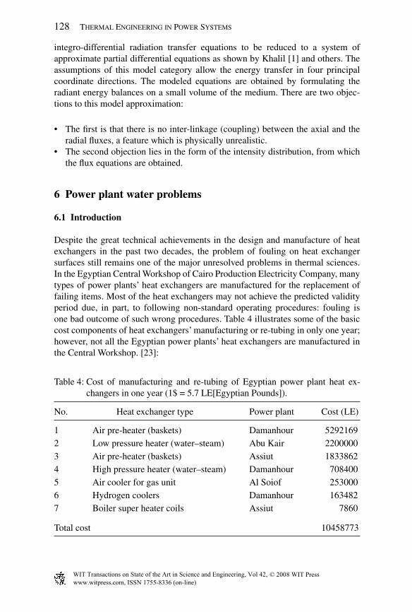
Despite the great technical achievements in the design and manufacture of heat exchangers in the past two decades, the problem of fouling on heat exchanger surfaces still remains one of the major unresolved problems in thermal sciences. In the Egyptian Central Workshop of Cairo Production Electricity Company, many types of power plants’ heat exchangers are manufactured for the replacement of failing items. Most of the heat exchangers may not achieve the predicted validity period due, in part, to following non-standard operating procedures: fouling is one bad outcome of such wrong procedures. Table 4 illustrates some of the basic cost components of heat exchangers’ manufacturing or re-tubing in only one year; however, not all the Egyptian power plants’ heat exchangers are manufactured in the Central Workshop. [23]:

Table 4: Cost of manufacturing and re-tubing of Egyptian power plant heat ex-changers in one year (1$ = 5.7 LE[Egyptian Pounds]).

No. Heat exchanger type Power plant Cost (LE)

1 Air pre-heater (baskets) Damanhour 52921692 Low pressure heater (water–steam) Abu Kair 22000003 Air pre-heater (baskets) Assiut 18338624 High pressure heater (water–steam) Damanhour 7084005 Air cooler for gas unit Al Soiof 2530006 Hydrogen coolers Damanhour 1634827 Boiler super heater coils Assiut 7860

Total cost 10458773



6.2 What is fouling?

Fouling is generally defi ned as the accumulation of undesired deposits of materi-als on the surfaces of processing equipment. It has been recognized as a nearly universal problem in heat exchangers design and operation. It affects the operation of equipment in two ways:

The fouling layer has a low thermal conductivity. This increases the resistance • to heat transfer and reduces the effectiveness of heat exchangers – increasing temperature.As deposition occurs, the cross-sectional area is reduced, which causes an • increase in pressure drop across the apparatus.

Measurement of the fouling resistance is typically performed by measuring the total thermal resistance (1/UA) for the clean and fouled conditions. The fouling resistance (Rf) is obtained by subtraction of the 1/UA values for the fouled and clean conditions, respectively, giving:

Rf /A = 1/(UA)f – 1/(UA)c (17)

where A is the surface area on which the Rf is based. For tube side fouling, the UA values for the clean and fouled conditions are defi ned by eqns. (18) and (19), respectively:

1/(UA)c = 1/hiAi + tw/kwAw + 1/hoAo (18)

1/(UA)f = (1/hi + Rf )(1/Ai) + tw/kwAw + 1/hoAo (19)

The inside (hi) and outside (ho) heat transfer coeffi cients must be equal in the dirty and clean tube conditions. Otherwise, the measured fouling resistance Rf will be erroneous.

6.3 Types of fouling

Fouling research has resulted in the defi nition of six different types of fouling that may occur with liquid or gases:

Precipitation fouling (scaling) • is the most common form of fouling and is associ-ated with inverse solubility salts. Examples of such salts are CaCO3, CaSO4, Ca3(PO4)2, CaSiO3, Ca(OH)2, Mg(OH)2, MgSiO3, Na2SO4, LiSO4, and Li2CO3. The characteristic which is termed inverse solubility is that, unlike most inor-ganic materials, the solubility decreases with temperature. The most important of these compounds is calcium carbonate, CaCO3. Calcium carbonate exists in several forms, but one of the more important is limestone. Running primarily through openings in limestone rock, it becomes saturated with calcium carbonate. Water pumped from the ground and passed through a water heater becomes



supersaturated as it is heated, and so CaCO3 begins to crystallize on the internal passages. Similar results occur when ground water is used in any industrial cooling process. The material frequently crystallizes in a form closely resem-bling marble, another form of calcium carbonate. Such materials are extremely diffi cult to remove mechanically and may require acid cleaning.Corrosion fouling• is classifi ed as a chemical reaction, which involves the heat exchanger tubes. Many metals, copper and aluminum being specifi c examples, form adherent oxide coatings which serve to passivate the surface and prevent further corrosion. Metal oxides are a type of ceramic and typically exhibit quite low thermal conductivities. Even relative thin coatings of oxides may signifi -cantly affect heat exchanger performance and should be included in evaluating overall heat transfer resistance.Chemical reaction fouling• involves chemical reactions in the process stream which results in deposition of material on the heat exchanger tubes. When food products are involved, this may be termed scorching but a wide range of or-ganic materials are subject to similar problems. This is commonly encountered when chemically sensitive process fl uids are heated to temperatures near that for chemical decomposition. Because of the non-fl ow conditions at the wall surface and the temperature gradient, which exists across this laminar sub–layer, these regions will operate at somewhat higher temperatures than the bulk and are ideally suited to promote favorable conditions for such reactions.Freezing fouling• is said to occur when a portion of the hot stream is cooled to near the freezing point for one of its components. This is most notable in refi n-eries where paraffi n frequently solidifi es from petroleum products at various stages in the refi ning process, obstructing both fl ow and heat transfer.Biological fouling• is common where untreated water is used as a coolant stream. Problems range from alga or other microbes to barnacles. During the season when such microbes are said to bloom, colonies several millimeters deep may grow across a tube surface virtually overnight, impeding circulation near the tube wall and retarding heat transport. Viewed under a microscope, many of these organisms appear as loosely intertwined fi bers – much like the form of fi berglass insulation. Traditionally, these organisms have been treated which chlorine, but the present day concerns on possible contamination to open water bodies have severely restricted the use of oxidizers in open discharge systems.Particulate fouling (sedimentation)• results from the presence of Brownian-sized particles in solution. Under certain conditions, such materials display a phenomenon known as thermophoresis in which motion is induced as a result of a temperature gradient. Thermodynamically this is referred to as a cross-coupled phenomenon and may be viewed as being analogous to the sea beck effect. When such particles accumulate on a heat exchanger surface they sometimes fuse, resulting in a build-up having the texture of sandstone. Like scale, these deposits are diffi cult to remove mechanically. Most of the actual data on fouling factors are tightly held by a few specialty consulting compa-nies. The data which are commonly available are sparse. An example is demonstrated in Table 5.



6.4 Fouling fundamentals

Fouling is a rate-dependent phenomenon. The net fouling rate is the difference between the solids deposition rate and their removal rate:

dmf /dt = md – mr (20)

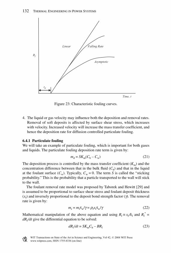
Depending on the magnitudes of the deposition and removal terms, several fouling rate characteristics are possible. Figure 23 illustrates the increase of the fouling factor (Rf) with time for different possible fouling situations. Crystallization foul-ing has an initial delay period (td), during which nucleation sites are established; then, the fouling deposit begins to accumulate. A linear growth of the fouling deposit occurs if the removal rate (mr) is negligible or if md and mr are constant with md > m.

α . Crystallization, chemical reaction, corrosion, and freezing foul-ing will show behavior in the linear or falling rate categories. The fouling resis-tance will attain an asymptotic value if md is constant and mr eventually attains a constant value. Particulate fouling typically shows asymptotic behavior. Which type of fouling characteristics occurs depends on the fouling mechanism.

References [25–28] provide a detailed discussion of the different fouling mech-anisms, these also describe the models to predict the deposition and removal rates for the different fouling mechanisms.The deposition model is a function of the fouling mechanism. The removal rate model depends on the re-entrainment rate, which is proportional to the shear stress at the surface. The heat exchanger operat-ing parameters that may infl uence the deposition or removal rates are as follows:

1. The bulk fl uid temperature will typically increase chemical reaction rates and crystallization deposition rates.

2. Increasing surface temperature will increase chemical reaction rates, or crystal-lization from inverse solubility salts. Reducing surface temperature will increase solidifi cation fouling.

3. The combination of surface material and fl uid will infl uence corrosion fouling. Copper surfaces act as a biocide to biological fouling. Rough surfaces may promote nucleation based phenomena.

Table 5: Representative fouling factors [24].

Fluid ′′fR (m2 K/W)

Seawater and treated boiler feed water (below 50°C) 0.0001Seawater and treated boiler feed water (above 50°C) 0.0002River water (below 50°C) 0.0002–0.001Fuel oil 0.0009Refrigerating liquids 0.0002Steam (non-oil bearing) 0.0001



4. The liquid or gas velocity may infl uence both the deposition and removal rates. Removal of soft deposits is affected by surface shear stress, which increases with velocity. Increased velocity will increase the mass transfer coeffi cient, and hence the deposition rate for diffusion controlled particulate fouling.

6.4.1 Particulate foulingWe will take an example of particulate fouling, which is important for both gases and liquids. The particulate fouling deposition rate term is given by:

md = SKm(Cb – Cw) (21)

The deposition process is controlled by the mass transfer coeffi cient (Km) and the concentration difference between that in the bulk fl uid (Cb) and that in the liquid at the foulant surface (Cw). Typically, Cw = 0. The term S is called the “sticking probability.” This is the probability that a particle transported to the wall will stick to the wall.

The foulant removal rate model was proposed by Taborek and Hewitt [29] and is assumed to be proportional to surface shear stress and foulant deposit thickness (xf) and inversely proportional to the deposit bond strength factor (γ). The removal rate is given by:

mr = mfτw/γ = ρfxfτw/γ (22)

Mathematical manipulation of the above equation and using Rf ≡ xf /kf and Rf* =

dRf /dt give the differential equation to be solved:

dRf /dt = SKmCb – BRf (23)

Linear Falling Rate

Rf

Asymptotic

td

Time, t

Figure 23: Characteristic fouling curves.



where

B = ρfxfτw/γ (24)

The resulting fouling resistance is given as:

Rf = Rf*(1 – e–Bt) (25)

where Rf* is the asymptotic fouling resistance defi ned by:

Rf* = SKmCb/B (26)

Equations (25) and (26) show that the Rf and Rf* can be predicted if Km, τw, S, and

γ are known. One must also know the foulant density (ρf) and thermal conductivity (kf). The values of S and γ were unity. Three different regimes for particle deposi-tion these are diffusion, inertia, and impaction regimes. Which regime controls the deposition process is determined by the dimensionless particle relaxation time defi ned by:

t+ = ρpd2(u*)2/18µv (27)

The values of t* associated with the diffusion, inertia, and impaction regimes are t+ < 0.10 (diffusion). 0.10 ≤ t+ ≤ 10 (inertia), and t+ > 10 (impaction). Fine- particle transport will probably be diffusion controlled. For example, the deposition process will be diffusion controlled for dp ≤ 10 μm for Re = 30,000 in a 15-mm-diameter tube. If the particle transport is diffusion-controlled, the mass transfer coeffi cient may be predicted from heat transfer data on the enhanced surface, using the heat-mass transfer analogy, as reported [28, 29] on rough surfaces. If the heat transfer coeffi cient for the enhanced surface (h) is known, the mass transfer coeffi cient can be calculated. Small particles result in high Schmidt numbers; a high heat transfer coeffi cient will result in a high mass transfer coeffi cient. Hence, enhanced heat transfer surfaces should result in higher foulant deposition rates than those occurring with plain surfaces at the same operating velocity.

6.5 Fouling mitigation, control and removal techniques

For many years, fouling has been considered an unavoidable and unresolved prob-lem besides being human responsibility. Owing to the enormous cost associated with fouling, a considerable number of fouling mitigation strategies have been developed. Fouling is a function of many variables. For example, fouling in crude oil heat exchangers is affected by oil composition, inorganic contaminates, pro-cess conditions (temperature, pressure fl ow rate, etc), exchanger and piping con-fi guration and surface temperature, etc. Therefore, as an effective control of these variables certain conditions may minimize fouling. Generally, effective fouling control methods should involve:

Preventive fouling formation.• Preventive foulant from adherence to heat transfer surfaces.• Removal of deposits from these surfaces.•



6.5.1 Confi guration of heat exchangerAn excess heat transfer surface area that is considered in design to cope with fouling can be as much 10–500%. However, this does not prevent deposition of fouling. At best, it increases the operation time between cleaning cycles. The depo-sition of dirt on heat transfer surfaces can be greatly reduced by proper design and selection of heat exchangers.

6.5.2 Reduction of fouling concentrationFouling generally increases with increasing foulant concentration in fl owing fl uids. Filtration, fl occulation and sedimentation can remove particulate mat-ters. Reducing the attractive forces of deposition by dispersants and surfactants is also possible. Scaling species can be removed by ion exchange or by chemical treatments. For example, crude desalting to remove most of the solids and salts can reduce fouling in crude oil exchangers. Biofouling in cooling water systems can be reduced by micro-mesh fi lters to fi lter out the eggs and larvae of organisms.

6.5.3 Use of chemical additivesAntifoulants are widely used to control fouling. Most antifoulants have sev-eral functions, such as oxygen scavengers, metal deactivators and dispersants. For auto-oxidation including fouling, antioxidants can be added to absorb oxy-gen or react with oxidation products in a way to prevent the chain reaction of the auto-oxidation process. Metal deactivators are added to chelate metal ions, thereby preventing their catalytic effect on the auto-oxidation process. Once insoluble is formed by either auto-oxidation or thermal decomposition, dispersants can be added to minimize agglomeration of small insoluble polymeric or coke-like par-ticles or deposit, or sticking of particles to the tube wall. Antifouling chemicals are formulated from several materials. Some prevent foulant forming, while others prevent fouling from depositing on heat transfer equipment. Materials that pre-vent deposit formation include antioxidants, scale inhibitors, biocides, and cor-rosion inhibitors. Compounds that prevent deposition are surfactants that act as detergents or dispersants. Different combinations of these properties are blended together to maximize results for different applications. These poly-functional anti-foulants are generally more versatile and effective since they can be designed to combat various types of fouling presented in any given system. Antifoulants are designed to prevent equipment surfaces from fouling, but they are not designed to clean up existing foulant. Therefore, antifoulants should be used immediately after cleaning of equipment. Many kinds of biocides, such as biguanides, phenol, formaldehyde and chlorine, etc. have been used to control bio fouling in industrial water systems. For different kinds of bacteria, it is essential to apply the correct biocides and dosages at the correct frequency.

6.5.4 High fl ow rate and low surface temperatureA well-established method of reducing fouling is to increase the wall shear stress by raising the fl ow velocity or by increasing the turbulence level. Temporarily, increasing



the fl ow velocity, reversing the fl ow direction and air rumbling are effective and inexpensive mitigation techniques, as long as the deposits are not too hard and adherent. The increase of fouling as the heat transfer temperature goes up is caused by increasing supersaturating, reaction rate, stickability or biological growth. Reducing the temperature usually leads to lower heat fl uxes and, therefore, larger heat exchangers. Increasing the velocity does not lead to high wall shear stress, but it leads to high fi lm coeffi cients and hence a desired lower surface temperature.

6.5.5 Chemical or mechanical cleaning of fouled process equipmentChemical cleaning often more effective than mechanical cleaning. In some cases, it can be done while the equipment is still in service. But the main disadvantage of chemical cleaning is the inability of the chemical solution to penetrate plugged tubes.

Mechanical cleaning, on the other hand, is a commonly used method to remove deposits from the shell side of heat exchanger tube bundles. In general, the bundles are fi rst pulled out, and then immersed in various chemical liquids to loosen or soften deposits. They are then subjected to a combination of high pressure hydro-blasting, rodding, sawing, scrapping, scratching, and in some cases an occasional light sandblasting [28].

6.5.6 Surfaces coatings and treatmentsThe relationship between surface energy and foulant adhesion has been intensively studied. It has been shown that the poorest foulant adhesion occurs on materials with low surface energies. Up to present, several low-energy coatings, for exam-ples, fl uoropolymers and silicone polymers, have been developed. Although the coated surfaces do accumulate fouling, the coatings themselves provide a signifi -cant additional resistance to heat transfer due to their low thermal conductivity, their use in heat exchangers limited. An effective method of bio fouling control is the application of antifouling coatings containing biocides with toxic properties to fouling organisms. The mechanism of surface protection by these paints upon control leads to poisonous ingredients.

Rough surfaces provide ideal nucleation sites for the growth and promote all types of fouling. The use of electro-polished stainless steel evaporator tubes in pulp and paper, chemical and food processing industries allows longer operation periods between cleaning cycles. If the heat transfer resistance of the tube material is not the major problem, polypropylene tubing, or glass-lined tubing can be used.

6.5.6.1 Scheduling cleaning The functions of cleaning exchangers are to permit thorough inspection and to remove foulant and scale that have reduced their per-formance. Plant designers try to match deterioration and fouling rates of system components so that no single one limits output. However, corrosion, erosion, and fouling rates vary with the fl uids fl owing, and their concentrations, fl ow rates, and temperatures. Furthermore, since temperatures and concentrations in a given fl uid nearly always change as the fl uid passes through the system, deterioration



rates and fouling build-up often vary with the location of a piece of equipment. In a tubular heat exchanger, the rates of deterioration and fouling may vary across the whole unit. An example is a multipass unit with hot fl uid entering the tubes that suffer more corrosion in the inlet pass than in the outlet one. An example of a fouled boiler tube surface is shown in Fig. 24.

Cleaning the tube and shell sides of heat exchangers requires taking into account the fouling. The following procedure is suggested as a basis for scheduling cleaning in which fouling is deposited from cooling-tower water as indicated in Fig. 25:

1. Achieve steady-state operation. 2. Measure the four terminal temperatures and pressures and the fl ow rate on

each side. 3. Calculate the clean overall coeffi cient and actual shell- and tube-side pres-

sures drop. 4. Repeat the measurements and calculations at regular intervals. Measurements

and calculations may be made manually, or automatically using a fouling monitor setup.

5. Calculate the fouling rate. 6. Plot the fouling resistance against time. 7. If there is a time delay before the onset of measurable fouling, relocate the

origin of the plot to set time zero at the onset point.

Figure 24: Example of fouled water tube furnace wall [23].



8. Extrapolate the plot as a linear falling rate or asymptotic rate to the point of intersection with the design fouling allowance.

9. Plan to clean at the time shown by the intersection point.10. Continue to monitor to refi ne the extrapolation.11. After cleaning, repeat the process to establish a cycle.12. Alternatively, plot the rate of pressure-drop build-up.

Figure 25 is a plot of fouling resistance with time for three kinds of industrial cooling water fouling. In linear fouling, resistance to heat fl ow increases linearly with time. This indicates that the shear force of the water on the foulant never becomes great enough to peel off accreted layers. In falling-rate fouling, shear forces due to fl ow make it increasingly diffi cult for layers to build up. Asymptotic fouling is the desired type. Here, the rate of shear approaches the rate of accumula-tion at the design fouling allowance. The fourth curve is a generalization for any of the types when acid cleaning fl uid is injected into cooling-tower water to remove deposits.

To set a schedule, the scheduler needs some idea of the work to be done, who will do it, and how long it will take. Furthermore, a logical sequence of doing the work must be prepared. The fi rst step is to make an on-line external inspection, including non-intrusive thickness measurements by ultrasonic scanning; the sec-ond is to examine the heat transfer characteristics of the equipments and compare with design values.

Figure 25: Variation of apparent differential fouling with time for industrial cooling waters.



7 Conclusions

The present chapter describes briefl y the basic concepts of powder genera-tion from Steam Power Plants and the more important factors that govern their performance as power cycles. Emphasis was placed on fossil fuel combustion in boiler furnaces and the various prevailing modeling assumptions. The main goal of effi cient power generation is, among others to rationalize the use of fossil fuels and enhance the combustion effi ciencies. The ability of numerical computations to predict the boiler furnace thermal behavior is an ultimate goal. The heat transfer to furnace walls through thermal radiation is reviewed briefl y to demonstrate the present capabilities. Boiler furnace walls are subject to major problem of fouling that deteriorate the performance and reduce the heat transfer characteristics dras-tically. The present work briefl y highlighted the fouling problem in Power plant water walls and proposes a monitoring, inspection and maintenance schedule.

References

[1] Khalil, E.E., Power Plant Design, Gordon and Breach: New York, USA, 1990. [2] Khalil, E.E., Modelling of Furnaces and Combustors, Abacus Press:

Tunbridge Wells, UK, 1983. [3] Khalil, E.E., Flow, Combustion & Heat Transfer in Axisymmetric Furnaces,

PhD Thesis, London University, 1977. [4] World Consumption of Primary Energy by Energy Type and Selected

Country Groups, 1980–2006 (XLS), Energy Information Administration, U.S. Department of Energy (July 31, 2006). Retrieved on 2007-01-20.

[5] Ministry of Electricity Annual Report, Egyptian Government, August 2007. [6] Khalil, E.E., Spalding, D.B. & Whitelaw, J.H., The calculation of local fl ow

properties in two-dimensional furnaces. International Journal of Heat and Mass Transfer, 18, pp. 775–792, 1975.

[7] Khalil, E.E., Numerical calculations of turbulent reaction rates in combus-tors, ASME 86-WA/HT-37, 1986.

[8] Khalil, E.E., Effect of swirl on fl ame characteristics in furnaces, AIAA paper AIAA-2004-5539, 2004.

[9] Launder, B.E. & Spalding, D.B., The numerical computation of turbulent fl ows. Computer Methods in Applied Mechanics and Engineering, 3(2), pp. 269–289, 1974.

[10] Gosman, A.D., Khalil, E.E. & Whitelaw, J.H., The Calculations of Two Dimensional Turbulent Recirculating Flows, Turbulent Shear Flows, Springer Verlag, pp. 13–35, 1979.

[11] Rodi, W.G., Turbulence Models and Their Applications in Hydraulics – A State of the Art Review, IAHR: Delft, Netherlands, 1984.

[12] Spalding, D.B. & Patankar, S.V., A calculation procedure for heat, mass and momentum transfer in three dimensional parabolic fl ows. International Jour-nal of Heat and Mass Transfer, 15, pp. 1787–1794, 1974.



[13] Gupta, A.K. & Lilley, D.G., Flow Field Modelling and Diagnostics, 1st edn, Abacus Press: Tunbridge Wells, UK, 1985.

[14] Borghi, R., Computational studies of turbulent fl ow with chemical reaction, Project SQUID on Turbulent Mixing, AGARD CP125, 1974.

[15] Khalil, E.E., On the modelling of reaction rates in turbulent premixed confi ned fl ames, AIAA–80-0015, 1980.

[16] Hutchinson, P., Khalil, E.E. & Whitelaw, J.H., The calculations of fl ow and heat transfer characteristics of gas fi red furnaces. Proc. 18th Symp. (Int.) on Combustion, pp. 1927–1931, 1980.

[17] Patankar, S.V., Numerical Heat Transfer and Fluid Flow, Hemisphere Publishing Corporation, Washington, DC, 1980.

[18] Henkes, R.W.M., Natural Convection Boundary Layers, PhD Thesis, Delft University, Netherlands,1990.

[19] Kameel, R. & Khalil, E.E., Heat transfer characteristics in furnaces: effect of combustion and heat transfer modelling, AIAA Paper, AIAA-2004-0803, January 2004.

[20] Kameel, R.A. & Khalil, E.E., Predictions of energy losses in furnaces under transient conditions. Proc. of the 3rd IECEC, San Francisco, AIAA-2005-5524, August 2005.

[21] Khalil, E.E. & Truelove, J.S., Calculations of heat transfer in a large gas fi red furnace. Letters in Heat and Mass Transfer, 4, pp. 353–365, 1977.

[22] Bartelds, H., Lewis, T.M., Michelfelder, S. & Pai, B.R., Prediction of radi-ant heat fl ux distribution in furnaces and its experimental testing, IFRF Doc.G02/a/23, 1973.

[23] Central Electrical Laboratory, Ministry of Electricity and Power, Egyptian Government, July 2005.

[24] ASME, Mechanical Engineering Handbook, ASME, 2005. [25] Panchal, C.B., Heat transfer monitor for measurements of fouling of industrial

heat exchangers, Symp. on Condenser Biofouling Control, Lake Buena Vista, Fla., Argonne National Lab., IL, June 1985.

[26] Somerscales, E.F.C., Fouling of Heat Transfer Equipment, ed. J.G. Knudsen, Hemisphere, December 1981.

[27] Förster, M. & Rumpf, B., Low fouling heat transfer surfaces for industri-al applications. Proceedings of the Heat Exchanger Fouling and Cleaning Fundamentals and Applications Conference, Santa Fe, New Mexico, USA, May 2003.

[28] Pugh, S., Hewitt, G.F. & Müller-Steinhagen, H., Fouling during the use of seawater as coolant – the development of a ‘User Guide’. Keynote Lecture, Proceedings of the Heat Exchanger Fouling and Cleaning Fundamentals and Applications Conference, Santa Fe, New Mexico, USA, May 2003.

[29] Taborek, J. & Hewitt, G.F., Advances in heat exchangers. Heat Exchangers: Theory and Practice, eds J. Taborek, G. Hewitt, & N.H. Afgan, Hemisphere Publishing Corp. and McGraw-Hill, pp. 979–990, 1983.


Documents

CHAPTER 4 Steam power plants - WIT Press · CHAPTER 4 Steam power plants E. Khalil Department of Mechanical Power Engineering, Cairo University, Cairo, Egypt. Abstract The efﬁ cient