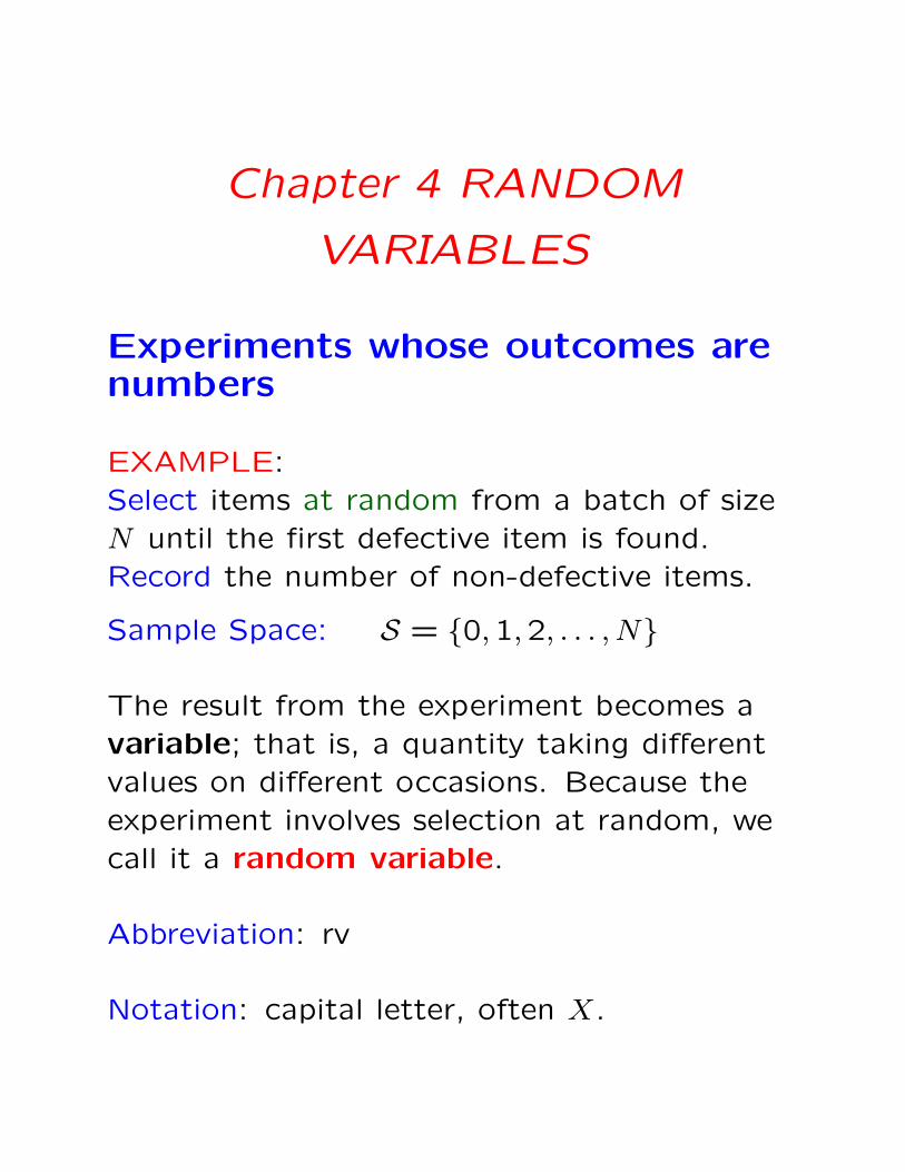
Chapter 4 RANDOM

VARIABLES

Experiments whose outcomes arenumbers

EXAMPLE:Select items at random from a batch of sizeN until the first defective item is found.Record the number of non-defective items.

Sample Space: S = {0,1,2, . . . , N}

The result from the experiment becomes avariable; that is, a quantity taking differentvalues on different occasions. Because theexperiment involves selection at random, wecall it a random variable.

Abbreviation: rv

Notation: capital letter, often X.

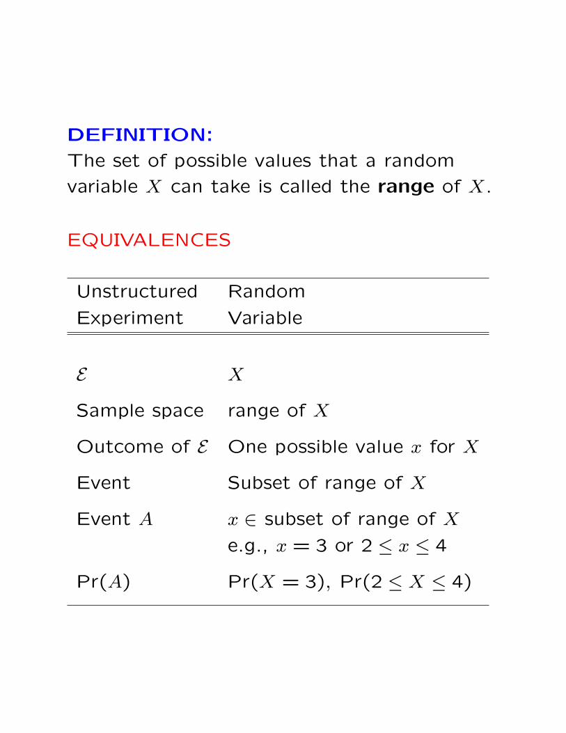
DEFINITION:

The set of possible values that a random

variable X can take is called the range of X.

EQUIVALENCES

Unstructured Random

Experiment Variable

E X

Sample space range of X

Outcome of E One possible value x for X

Event Subset of range of X

Event A x ∈ subset of range of X

e.g., x = 3 or 2 ≤ x ≤ 4

Pr(A) Pr(X = 3), Pr(2 ≤ X ≤ 4)

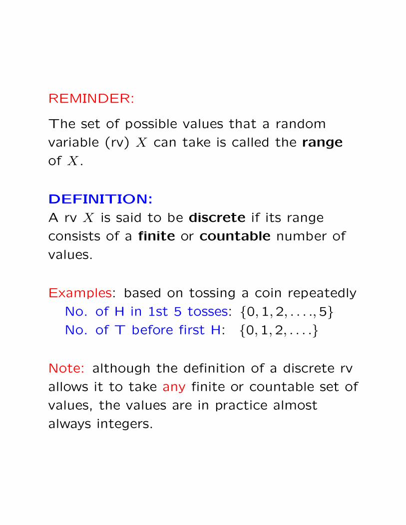
REMINDER:

The set of possible values that a random

variable (rv) X can take is called the range

of X.

DEFINITION:

A rv X is said to be discrete if its range

consists of a finite or countable number of

values.

Examples: based on tossing a coin repeatedly

No. of H in 1st 5 tosses: {0,1,2, . . . .,5}No. of T before first H: {0,1,2, . . . .}

Note: although the definition of a discrete rv

allows it to take any finite or countable set of

values, the values are in practice almost

always integers.

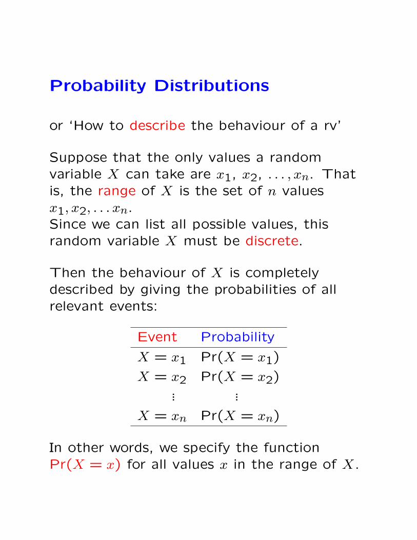
Probability Distributions

or ‘How to describe the behaviour of a rv’

Suppose that the only values a randomvariable X can take are x1, x2, . . . , xn. Thatis, the range of X is the set of n valuesx1, x2, . . . xn.Since we can list all possible values, thisrandom variable X must be discrete.

Then the behaviour of X is completelydescribed by giving the probabilities of allrelevant events:

Event Probability

X = x1 Pr(X = x1)

X = x2 Pr(X = x2)... ...

X = xn Pr(X = xn)

In other words, we specify the functionPr(X = x) for all values x in the range of X.

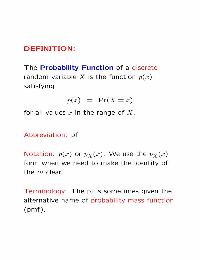
DEFINITION:

The Probability Function of a discrete

random variable X is the function p(x)

satisfying

p(x) = Pr(X = x)

for all values x in the range of X.

Abbreviation: pf

Notation: p(x) or pX(x). We use the pX(x)

form when we need to make the identity of

the rv clear.

Terminology: The pf is sometimes given the

alternative name of probability mass function

(pmf).

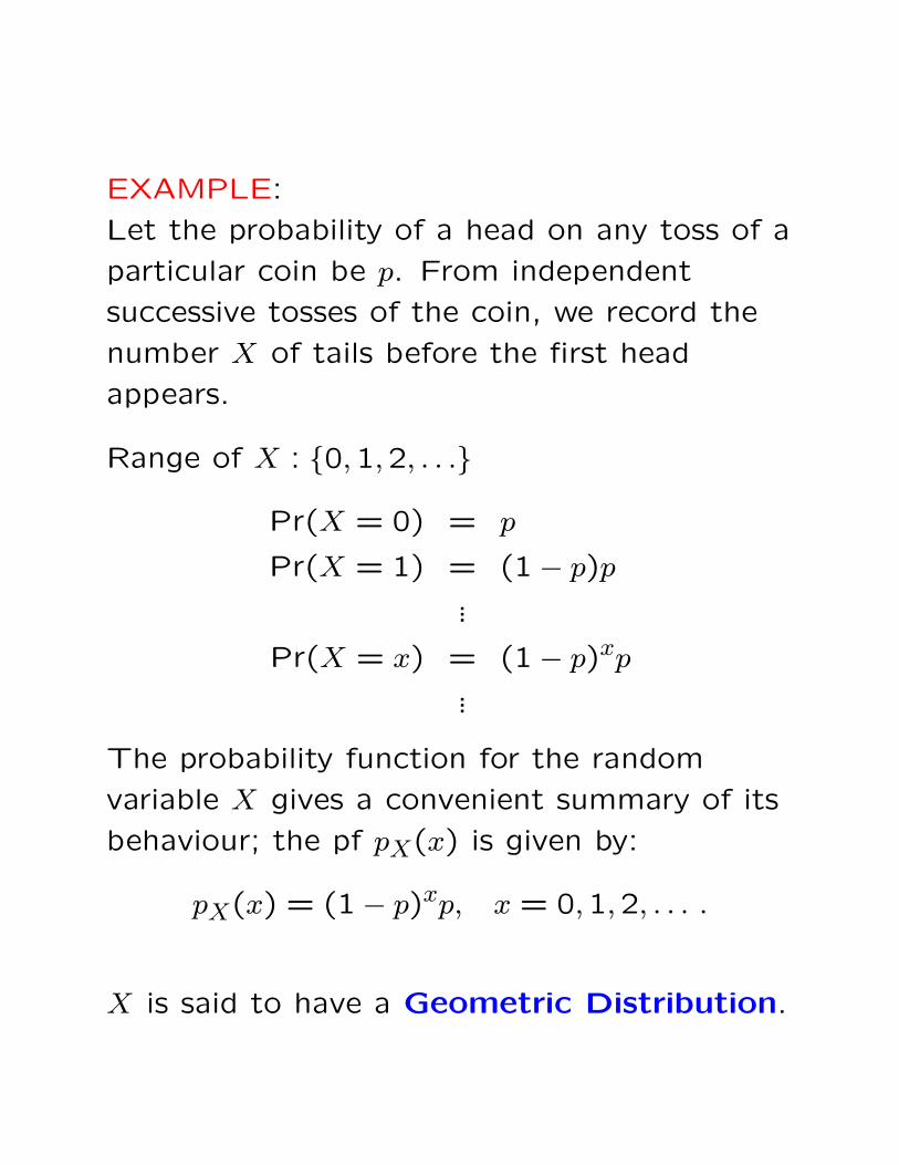
EXAMPLE:

Let the probability of a head on any toss of a

particular coin be p. From independent

successive tosses of the coin, we record the

number X of tails before the first head

appears.

Range of X : {0,1,2, . . .}

Pr(X = 0) = p

Pr(X = 1) = (1− p)p...

Pr(X = x) = (1− p)xp...

The probability function for the random

variable X gives a convenient summary of its

behaviour; the pf pX(x) is given by:

pX(x) = (1− p)xp, x = 0,1,2, . . . .

X is said to have a Geometric Distribution.

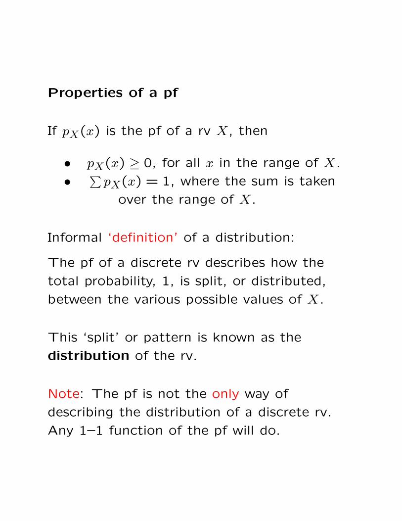
Properties of a pf

If pX(x) is the pf of a rv X, then

• pX(x) ≥ 0, for all x in the range of X.

•∑

pX(x) = 1, where the sum is taken

over the range of X.

Informal ‘definition’ of a distribution:

The pf of a discrete rv describes how the

total probability, 1, is split, or distributed,

between the various possible values of X.

This ‘split’ or pattern is known as the

distribution of the rv.

Note: The pf is not the only way of

describing the distribution of a discrete rv.

Any 1–1 function of the pf will do.

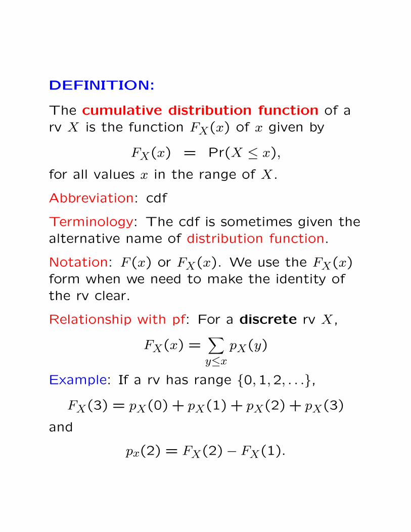
DEFINITION:

The cumulative distribution function of arv X is the function FX(x) of x given by

FX(x) = Pr(X ≤ x),

for all values x in the range of X.

Abbreviation: cdf

Terminology: The cdf is sometimes given thealternative name of distribution function.

Notation: F (x) or FX(x). We use the FX(x)form when we need to make the identity ofthe rv clear.

Relationship with pf: For a discrete rv X,

FX(x) =∑y≤x

pX(y)

Example: If a rv has range {0,1,2, . . .},

FX(3) = pX(0) + pX(1) + pX(2) + pX(3)

and

px(2) = FX(2)− FX(1).

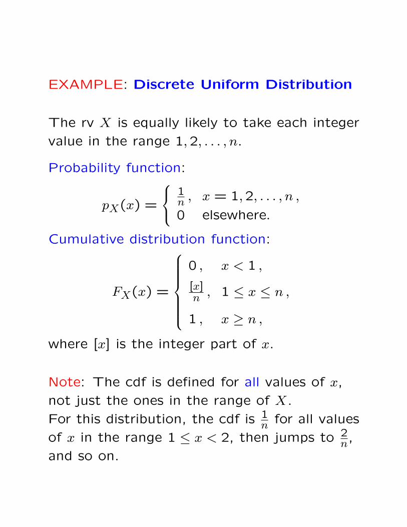
EXAMPLE: Discrete Uniform Distribution

The rv X is equally likely to take each integer

value in the range 1,2, . . . , n.

Probability function:

pX(x) =

1n , x = 1,2, . . . , n ,

0 elsewhere.

Cumulative distribution function:

FX(x) =

0 , x < 1 ,

[x]n , 1 ≤ x ≤ n ,

1 , x ≥ n ,

where [x] is the integer part of x.

Note: The cdf is defined for all values of x,

not just the ones in the range of X.

For this distribution, the cdf is 1n for all values

of x in the range 1 ≤ x < 2, then jumps to 2n,

and so on.

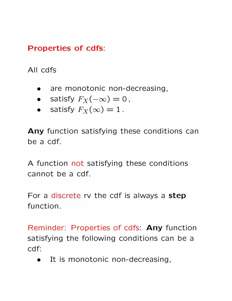
Properties of cdfs:

All cdfs

• are monotonic non-decreasing,

• satisfy FX(−∞) = 0 ,

• satisfy FX(∞) = 1 .

Any function satisfying these conditions can

be a cdf.

A function not satisfying these conditions

cannot be a cdf.

For a discrete rv the cdf is always a step

function.

Reminder: Properties of cdfs: Any function

satisfying the following conditions can be a

cdf:

• It is monotonic non-decreasing,

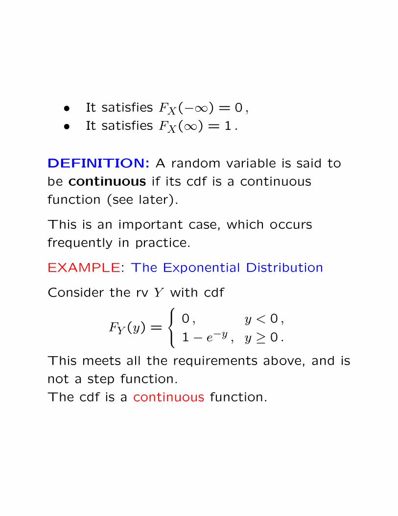
• It satisfies FX(−∞) = 0 ,

• It satisfies FX(∞) = 1 .

DEFINITION: A random variable is said to

be continuous if its cdf is a continuous

function (see later).

This is an important case, which occurs

frequently in practice.

EXAMPLE: The Exponential Distribution

Consider the rv Y with cdf

FY (y) =

0 , y < 0 ,

1− e−y , y ≥ 0 .

This meets all the requirements above, and is

not a step function.

The cdf is a continuous function.

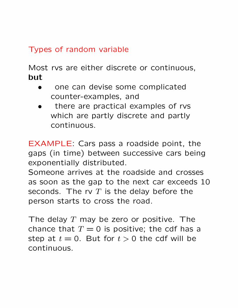
Types of random variable

Most rvs are either discrete or continuous,but• one can devise some complicated

counter-examples, and• there are practical examples of rvs

which are partly discrete and partlycontinuous.

EXAMPLE: Cars pass a roadside point, thegaps (in time) between successive cars beingexponentially distributed.Someone arrives at the roadside and crossesas soon as the gap to the next car exceeds 10seconds. The rv T is the delay before theperson starts to cross the road.

The delay T may be zero or positive. Thechance that T = 0 is positive; the cdf has astep at t = 0. But for t > 0 the cdf will becontinuous.

Mean and Variance

The pf gives a complete description of thebehaviour of a (discrete) random variable. Inpractice we often want a more concisedescription of its behaviour.

DEFINITION: The mean or expectation ofa discrete rv X, E(X), is defined as

E(X) =∑x

xPr(X = x).

Note: Here (and later) the notation∑x

means

the sum over all values x in the range of X.

The expectation E(X) is a weighted averageof these values. The weights always sum to 1.

Extension: The concept of expectation canbe generalised; we can define the expectationof any function of a rv. Thus we obtain, for afunction g(·) of a discrete rv X,

E{g(X)} =∑x

g(x)Pr(X = x) .

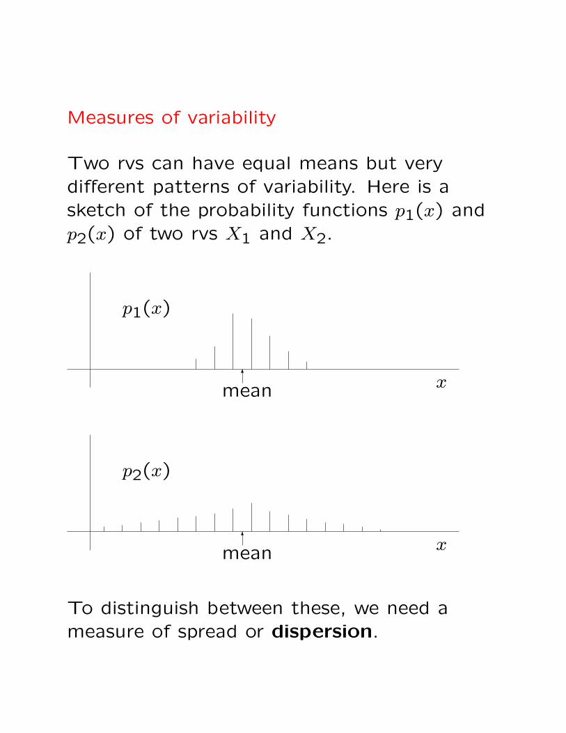
Measures of variability

Two rvs can have equal means but verydifferent patterns of variability. Here is asketch of the probability functions p1(x) andp2(x) of two rvs X1 and X2.

6

p1(x)

xmean

6

mean

p2(x)

x

To distinguish between these, we need ameasure of spread or dispersion.

Measures of dispersion

There are many possible measures. We look

briefly at three plausible ones.

A. ‘Mean difference’: E{X − E(X)}.Attractive superficially, but no use.

B. Mean absolute difference: E{|X − E(X)|}.Hard to manipulate mathematically.

C. Variance: E{X − E(X)}2.

The most frequently-used measure.

Notation for variance: V(X) or Var(X).

That is: V(X) = Var(X) = E{X − E(X)}2.

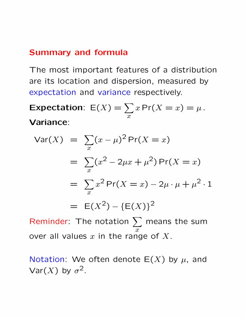
Summary and formula

The most important features of a distribution

are its location and dispersion, measured by

expectation and variance respectively.

Expectation: E(X) =∑x

xPr(X = x) = µ .

Variance:

Var(X) =∑x

(x− µ)2 Pr(X = x)

=∑x

(x2 − 2µx + µ2)Pr(X = x)

=∑x

x2 Pr(X = x)− 2µ · µ + µ2 · 1

= E(X2)− {E(X)}2

Reminder: The notation∑x

means the sum

over all values x in the range of X.

Notation: We often denote E(X) by µ, and

Var(X) by σ2.

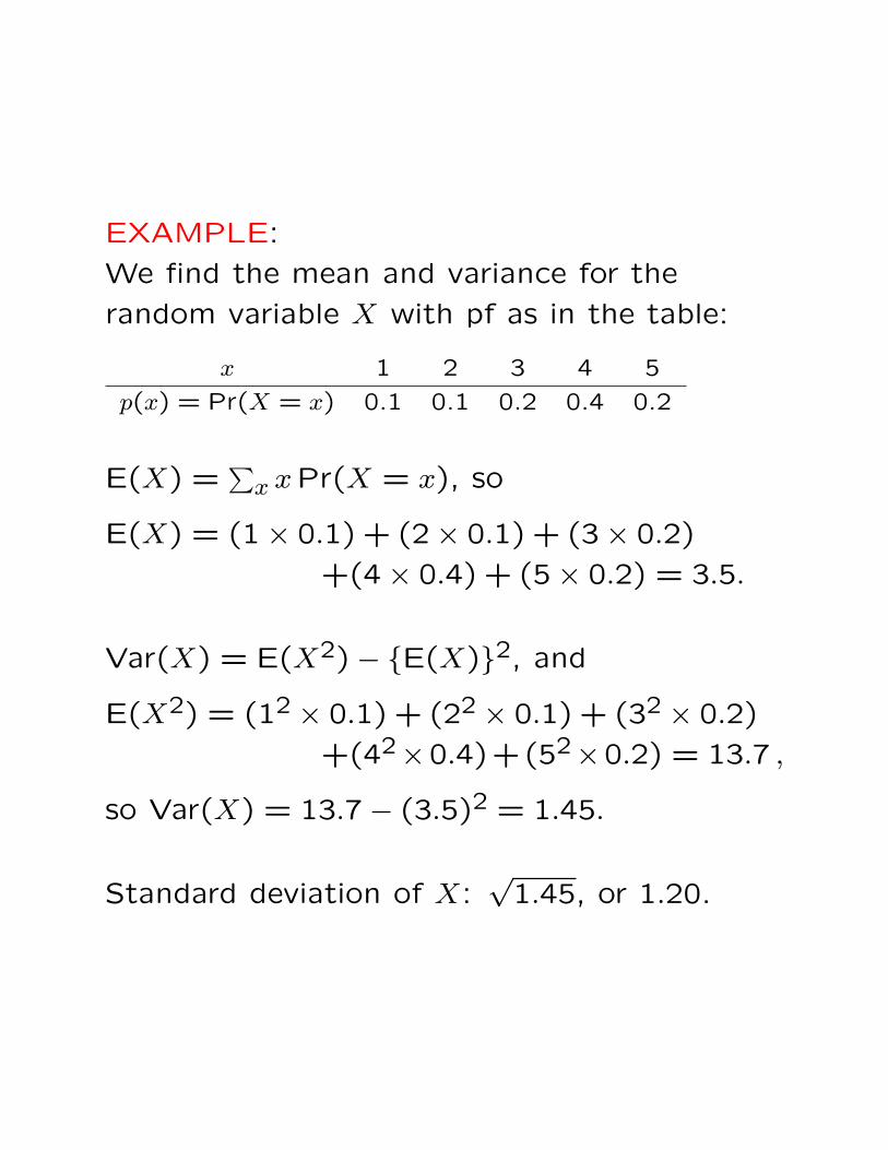
EXAMPLE:

We find the mean and variance for the

random variable X with pf as in the table:

x 1 2 3 4 5

p(x) = Pr(X = x) 0.1 0.1 0.2 0.4 0.2

E(X) =∑

x xPr(X = x), so

E(X) = (1× 0.1) + (2× 0.1) + (3× 0.2)

+(4× 0.4) + (5× 0.2) = 3.5.

Var(X) = E(X2)− {E(X)}2, and

E(X2) = (12 × 0.1) + (22 × 0.1) + (32 × 0.2)

+(42×0.4)+(52×0.2) = 13.7 ,

so Var(X) = 13.7− (3.5)2 = 1.45.

Standard deviation of X:√

1.45, or 1.20.

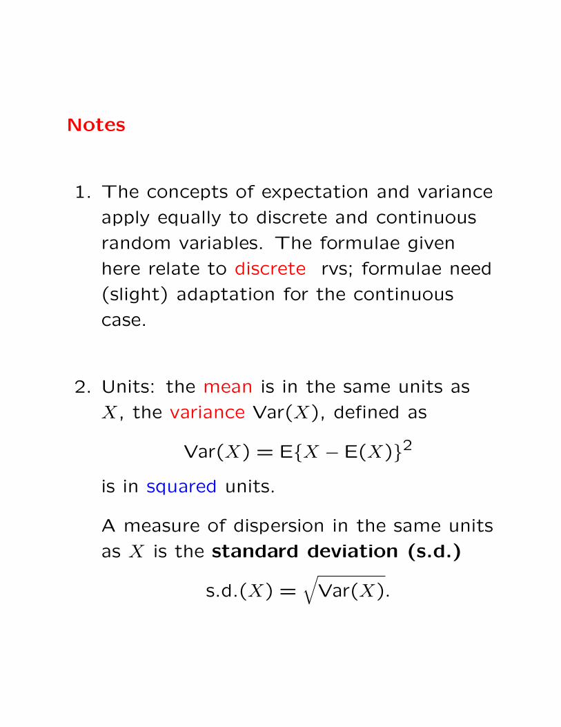
Notes

1. The concepts of expectation and variance

apply equally to discrete and continuous

random variables. The formulae given

here relate to discrete rvs; formulae need

(slight) adaptation for the continuous

case.

2. Units: the mean is in the same units as

X, the variance Var(X), defined as

Var(X) = E{X − E(X)}2

is in squared units.

A measure of dispersion in the same units

as X is the standard deviation (s.d.)

s.d.(X) =√

Var(X).

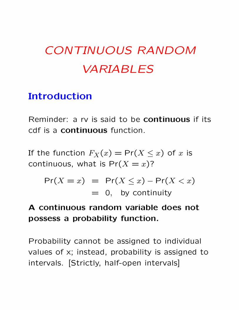
CONTINUOUS RANDOM

VARIABLES

Introduction

Reminder: a rv is said to be continuous if its

cdf is a continuous function.

If the function FX(x) = Pr(X ≤ x) of x is

continuous, what is Pr(X = x)?

Pr(X = x) = Pr(X ≤ x)− Pr(X < x)

= 0, by continuity

A continuous random variable does not

possess a probability function.

Probability cannot be assigned to individual

values of x; instead, probability is assigned to

intervals. [Strictly, half-open intervals]

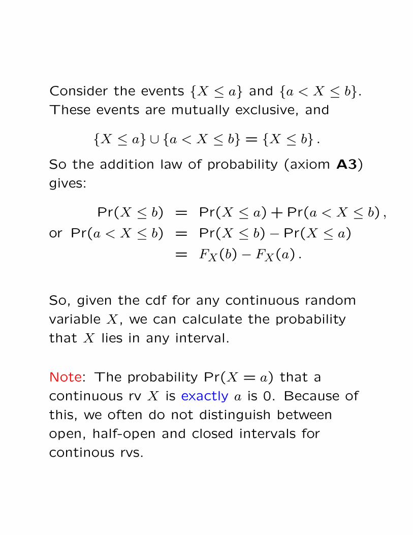
Consider the events {X ≤ a} and {a < X ≤ b}.These events are mutually exclusive, and

{X ≤ a} ∪ {a < X ≤ b} = {X ≤ b} .

So the addition law of probability (axiom A3)

gives:

Pr(X ≤ b) = Pr(X ≤ a) + Pr(a < X ≤ b) ,

or Pr(a < X ≤ b) = Pr(X ≤ b)− Pr(X ≤ a)

= FX(b)− FX(a) .

So, given the cdf for any continuous random

variable X, we can calculate the probability

that X lies in any interval.

Note: The probability Pr(X = a) that a

continuous rv X is exactly a is 0. Because of

this, we often do not distinguish between

open, half-open and closed intervals for

continous rvs.

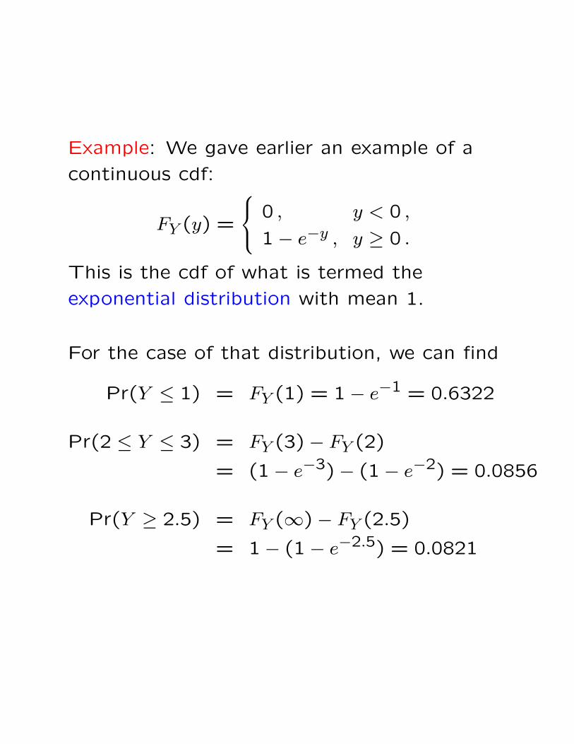
Example: We gave earlier an example of a

continuous cdf:

FY (y) =

0 , y < 0 ,

1− e−y , y ≥ 0 .

This is the cdf of what is termed the

exponential distribution with mean 1.

For the case of that distribution, we can find

Pr(Y ≤ 1) = FY (1) = 1− e−1 = 0.6322

Pr(2 ≤ Y ≤ 3) = FY (3)− FY (2)

= (1− e−3)− (1− e−2) = 0.0856

Pr(Y ≥ 2.5) = FY (∞)− FY (2.5)

= 1− (1− e−2.5) = 0.0821

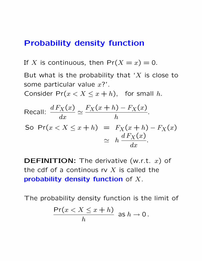
Probability density function

If X is continuous, then Pr(X = x) = 0.

But what is the probability that ‘X is close to

some particular value x?’.

Consider Pr(x < X ≤ x + h), for small h.

Recall:d FX(x)

dx'

FX(x + h)− FX(x)

h.

So Pr(x < X ≤ x + h) = FX(x + h)− FX(x)

' hd FX(x)

dx.

DEFINITION: The derivative (w.r.t. x) of

the cdf of a continous rv X is called the

probability density function of X.

The probability density function is the limit of

Pr(x < X ≤ x + h)

has h → 0 .

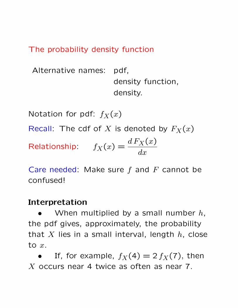
The probability density function

Alternative names: pdf,

density function,

density.

Notation for pdf: fX(x)

Recall: The cdf of X is denoted by FX(x)

Relationship: fX(x) =d FX(x)

dx

Care needed: Make sure f and F cannot be

confused!

Interpretation

• When multiplied by a small number h,

the pdf gives, approximately, the probability

that X lies in a small interval, length h, close

to x.

• If, for example, fX(4) = 2 fX(7), then

X occurs near 4 twice as often as near 7.

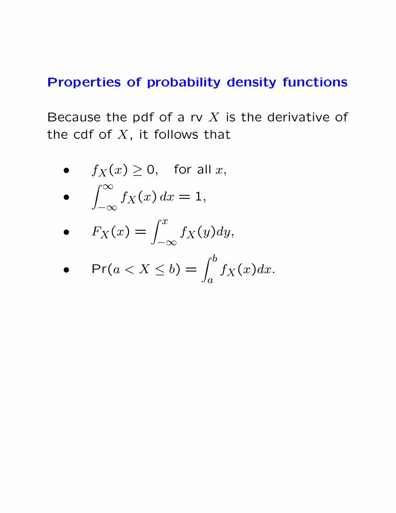
Properties of probability density functions

Because the pdf of a rv X is the derivative of

the cdf of X, it follows that

• fX(x) ≥ 0, for all x,

•∫ ∞

−∞fX(x) dx = 1,

• FX(x) =∫ x

−∞fX(y)dy,

• Pr(a < X ≤ b) =∫ b

afX(x)dx.

Mean and Variance

Reminder: for a discrete rv, the formulae formean and variance are based on theprobability function Pr(X = x). We need toadapt these formulae for use with continuousrandom variables.

DEFINITION:For a continuous rv X with pdf fX(x), theexpectation of a function g(x) is defined as

E{g(X)} =∫ ∞

−∞g(x) fX(x) dx

Hence, for the mean:

E(X) =∫ ∞

−∞x fX(x) dx

Compare this with the equivalent definitionfor a discrete random variable:

E(X) =∑x

xPr(X = x) , or E(X) =∑x

xpX(x) .

For the variance, recall the definition.

Var(X) = E[{X − E(X)}2]

Hence Var(X) =∫ ∞

−∞(x− µ)2 fX(x) dx

As in the discrete case, the best way to

caclulate a variance is by using the result:

Var(X) = E(X2)− {E(X)}2 .

In practice, we therefore usually calculate

E(X2) =∫ ∞

−∞x2 fX(x) dx

as a stepping stone on the way to obtaining

Var(X).

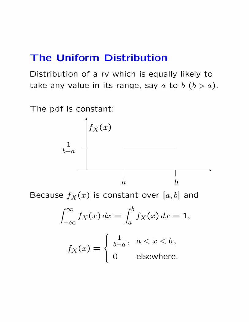
The Uniform Distribution

Distribution of a rv which is equally likely to

take any value in its range, say a to b (b > a).

The pdf is constant:6

-

a b

fX(x)

1b−a

Because fX(x) is constant over [a, b] and∫ ∞

−∞fX(x) dx =

∫ b

afX(x) dx = 1,

fX(x) =

1

b−a , a < x < b ,

0 elsewhere.

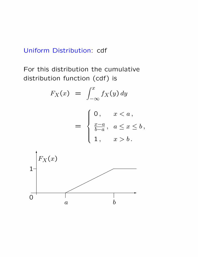
Uniform Distribution: cdf

For this distribution the cumulative

distribution function (cdf) is

FX(x) =∫ x

−∞fX(y) dy

=

0 , x < a ,

x−ab−a , a ≤ x ≤ b ,

1 , x > b .

6

-�����

�������

���

a b

FX(x)

1

0

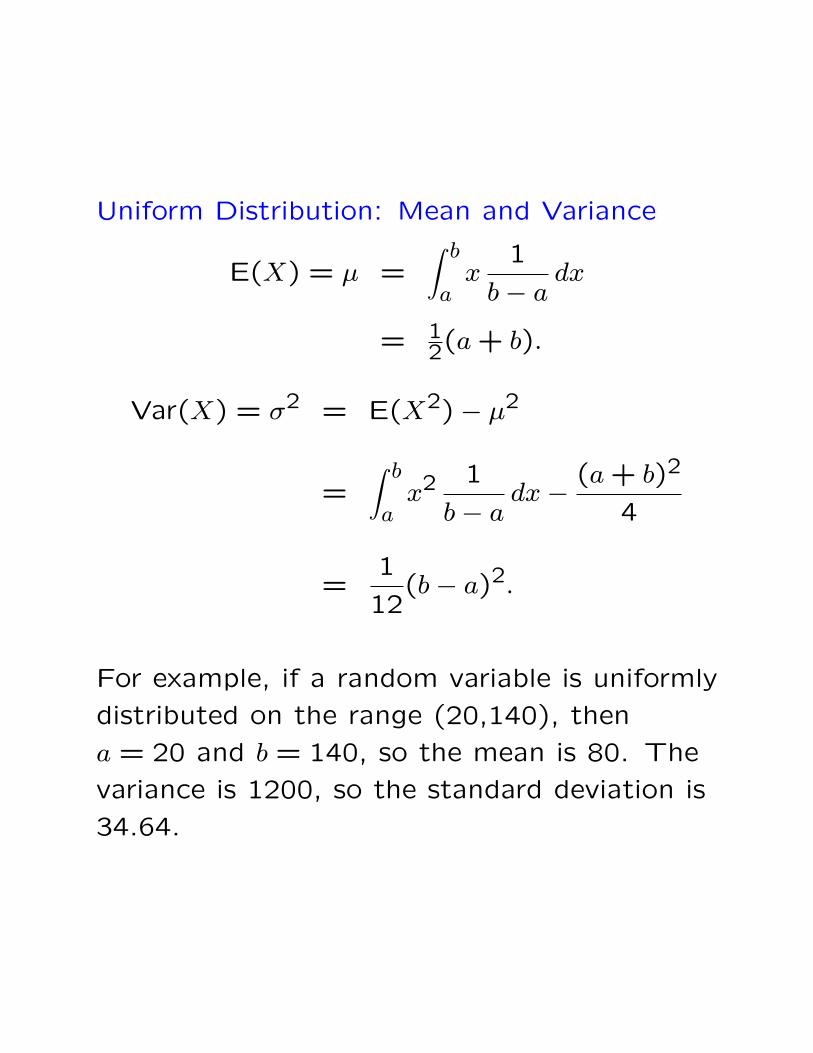
Uniform Distribution: Mean and Variance

E(X) = µ =∫ b

ax

1

b− adx

= 12(a + b).

Var(X) = σ2 = E(X2)− µ2

=∫ b

ax2 1

b− adx−

(a + b)2

4

=1

12(b− a)2.

For example, if a random variable is uniformly

distributed on the range (20,140), then

a = 20 and b = 140, so the mean is 80. The

variance is 1200, so the standard deviation is

34.64.

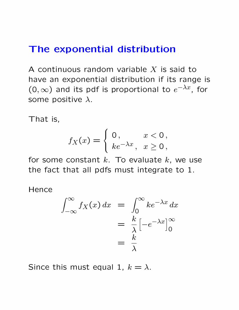
The exponential distribution

A continuous random variable X is said tohave an exponential distribution if its range is(0,∞) and its pdf is proportional to e−λx, forsome positive λ.

That is,

fX(x) =

0 , x < 0 ,

ke−λx , x ≥ 0 ,

for some constant k. To evaluate k, we usethe fact that all pdfs must integrate to 1.

Hence ∫ ∞

−∞fX(x) dx =

∫ ∞

0ke−λx dx

=k

λ

[−e−λx

]∞0

=k

λ

Since this must equal 1, k = λ.

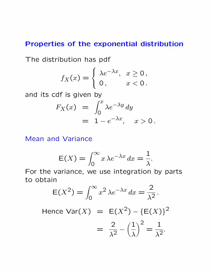
Properties of the exponential distribution

The distribution has pdf

fX(x) =

λe−λx, x ≥ 0 ,

0 , x < 0 .

and its cdf is given by

FX(x) =∫ x

0λe−λy dy

= 1− e−λx, x > 0 .

Mean and Variance

E(X) =∫ ∞

0x λe−λx dx =

1

λ.

For the variance, we use integration by partsto obtain

E(X2) =∫ ∞

0x2 λe−λx dx =

2

λ2.

Hence Var(X) = E(X2)− {E(X)}2

=2

λ2−

(1

λ

)2=

1

λ2.

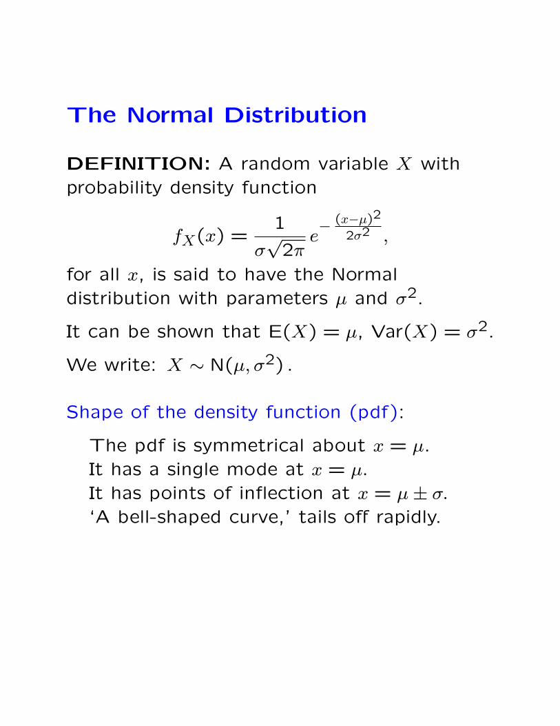
The Normal Distribution

DEFINITION: A random variable X withprobability density function

fX(x) =1

σ√

2πe− (x−µ)2

2σ2 ,

for all x, is said to have the Normaldistribution with parameters µ and σ2.

It can be shown that E(X) = µ, Var(X) = σ2.

We write: X ∼ N(µ, σ2) .

Shape of the density function (pdf):

The pdf is symmetrical about x = µ.It has a single mode at x = µ.

It has points of inflection at x = µ± σ.

‘A bell-shaped curve,’ tails off rapidly.

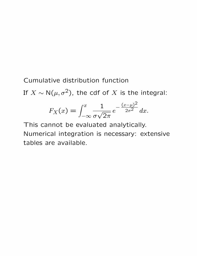
Cumulative distribution function

If X ∼ N(µ, σ2), the cdf of X is the integral:

FX(x) =∫ x

−∞

1

σ√

2πe− (x−µ)2

2σ2 dx.

This cannot be evaluated analytically.

Numerical integration is necessary: extensive

tables are available.

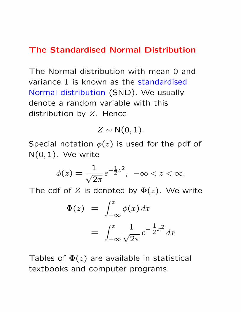
The Standardised Normal Distribution

The Normal distribution with mean 0 and

variance 1 is known as the standardised

Normal distribution (SND). We usually

denote a random variable with this

distribution by Z. Hence

Z ∼ N(0,1).

Special notation φ(z) is used for the pdf of

N(0,1). We write

φ(z) =1√2π

e−12z2

, −∞ < z < ∞.

The cdf of Z is denoted by Φ(z). We write

Φ(z) =∫ z

−∞φ(x) dx

=∫ z

−∞

1√2π

e−12x2

dx

Tables of Φ(z) are available in statistical

textbooks and computer programs.

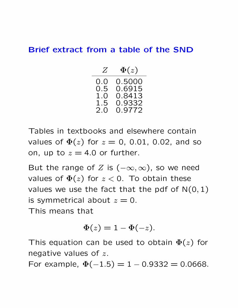
Brief extract from a table of the SND

Z Φ(z)

0.0 0.50000.5 0.69151.0 0.84131.5 0.93322.0 0.9772

Tables in textbooks and elsewhere contain

values of Φ(z) for z = 0, 0.01, 0.02, and so

on, up to z = 4.0 or further.

But the range of Z is (−∞,∞), so we need

values of Φ(z) for z < 0. To obtain these

values we use the fact that the pdf of N(0,1)

is symmetrical about z = 0.

This means that

Φ(z) = 1−Φ(−z).

This equation can be used to obtain Φ(z) for

negative values of z.

For example, Φ(−1.5) = 1− 0.9332 = 0.0668.