Chapter 16 Continuous Random Variables

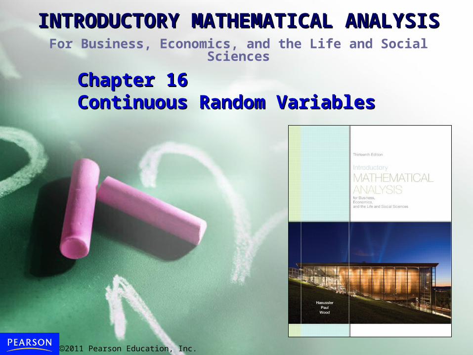
INTRODUCTORY MATHEMATICAL INTRODUCTORY MATHEMATICAL ANALYSISANALYSISFor Business, Economics, and the Life and Social Sciences

2011 Pearson Education, Inc.

Chapter 16 Chapter 16 Continuous Random VariablesContinuous Random Variables


• To introduce continuous random variables and discuss density functions.

• To discuss the normal distribution, standard units, and the table of areas under the standard normal curve.

• To show the technique of estimating the binomial distribution by using normal distribution.

Chapter 16: Continuous Random Variables

Chapter ObjectivesChapter Objectives


Continuous Random Variables

The Normal Distribution

The Normal Approximation to the Binomial Distribution

16.1)

16.2)

16.3)


Chapter OutlineChapter Outline



16.1 Continuous Random Variables16.1 Continuous Random Variables

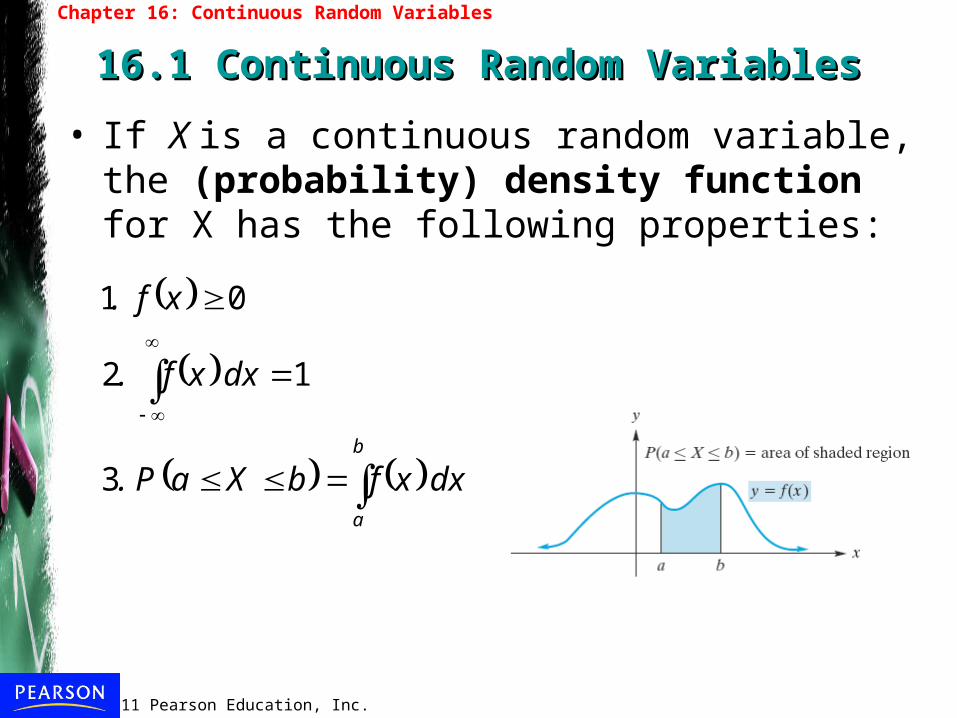
• If X is a continuous random variable, the (probability) density function for X has the following properties:

b

a

dxxfbXa. P

dxxf.

x. f

3

1 2

01



16.1 Continuous Random Variables

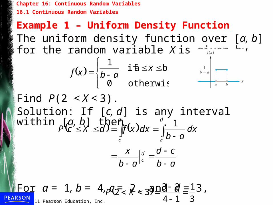
Example 1 – Uniform Density FunctionThe uniform density function over [a, b] for the random variable X is given by

Find P(2 < X < 3).Solution: If [c, d] is any interval within [a, b] then

For a = 1, b = 4, c = 2, and d = 3,

otherwise0

b a if1

xabxf

ab

cd

ab

x

dxab

dxxfdXcP

dc

d

c

d

c

1

3

1

14

2332

XP




Example 3 – Exponential Density FunctionThe exponential density function is defined by

where k is a positive constant, called a parameter, whose value depends on the experiment under consideration. If X is a random variable with this density function, then X is said to have an exponential distribution. Let k = 1. Then f(x) = e−x for x ≥ 0, and f(x) = 0 for x < 0.

0 if0

0 if

x

xkexf

kx




Example 3 – Exponential Density Function

a. Find P(2 < X < 3).

Solution:

b. Find P(X > 4).

Solution:

086.0)(

32

3223

32

3

2

eeee

edxeXP xx

018.001

lim

lim 4

44

44

eee

dxedxeXP

rr

rx

r

x




Example 5 – Finding the Mean and Standard DeviationIf X is a random variable with density function given by

find its mean and standard deviation.Solution:

otherwise 0

20 if 21 xx

xf

3

4

6

2

1 Mean,

2

0

32

0

xdxxxdxxxfμ

9

2

9

16

83

4

2

1

2

0

422

0

2222

xdxxxμdxxfxσ

3

2

9

2 Deviation, Standard



16.2 The Normal Distribution16.2 The Normal Distribution

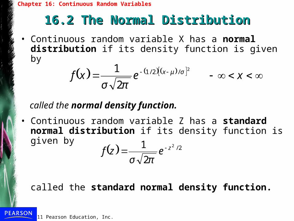
• Continuous random variable X has a normal distribution if its density function is given by

called the normal density function.

• Continuous random variable Z has a standard normal distribution if its density function is given by

called the standard normal density function.

xeπσ

xf σμx 2

1 2/2/1

2/2

2

1 zeπσ

zf



16.2 The Normal Distribution

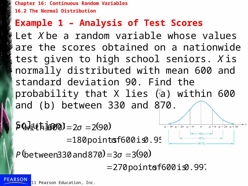
Example 1 – Analysis of Test Scores

Let X be a random variable whose values are the scores obtained on a nationwide test given to high school seniors. X is normally distributed with mean 600 and standard deviation 90. Find the probability that X lies (a) within 600 and (b) between 330 and 870.

Solution:

0.95 is 600 of points 180

9022600 within

σP

0.997 is 600 of points 270

9033870 and 330 between

σP



16.2 The Normal Distribution

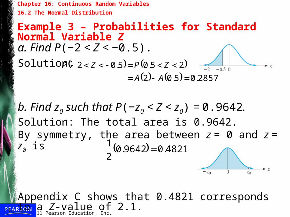
Example 3 – Probabilities for Standard Normal Variable Za. Find P(−2 < Z < −0.5).Solution:

b. Find z0 such that P(−z0 < Z < z0) = 0.9642.Solution: The total area is 0.9642. By symmetry, the area between z = 0 and z = z0 is

Appendix C shows that 0.4821 corresponds to a Z-value of 2.1.

2857.05.02

25.05.02

AA

ZPZP

4821.09642.02

1



16.3 The Normal Approximation to the 16.3 The Normal Approximation to the

Binomial DistributionBinomial Distribution

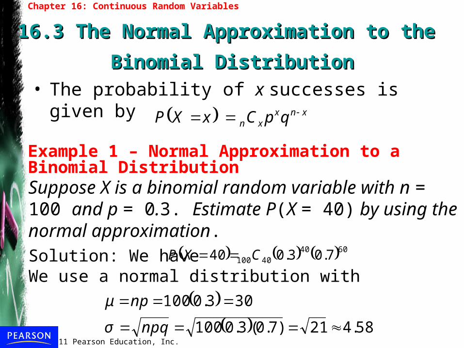
Example 1 – Normal Approximation to a Binomial Distribution

• The probability of x successes is given by

xnxxn qpCxXP

Suppose X is a binomial random variable with n = 100 and p = 0.3. Estimate P(X = 40) by using the normal approximation.Solution: We have We use a normal distribution with

604040100 7.03.040 CXP

58.421)7.0(3.0100

303.0100

npqσ

npμ



16.3 The Normal Approximation to the Binomial Distribution

Example 1 – Normal Approximation to a Binomial Distribution

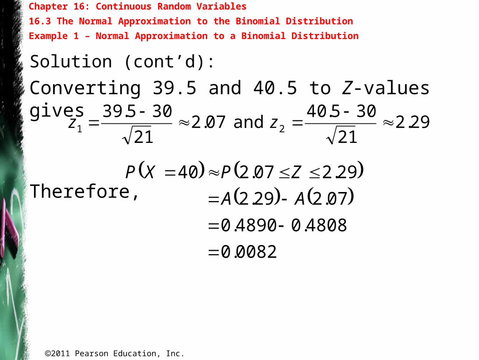
Solution (cont’d):

Converting 39.5 and 40.5 to Z-values gives

Therefore,

0082.0

4808.04890.0

07.229.2

29.207.240

AA

ZPXP

29.221

305.40 and 07.2

21

305.3921

zz

Documents

Chapter 16 Continuous Random Variables