Chapter 4 – Probability and Probability

Distributions

Sections 4.6 - 4.10

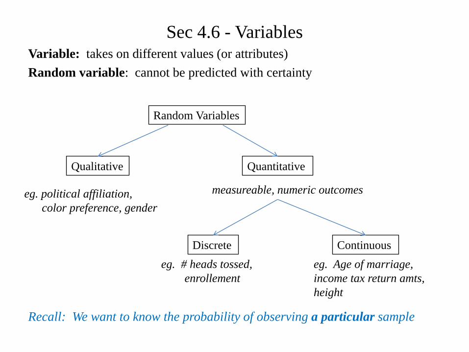
Sec 4.6 - VariablesVariable: takes on different values (or attributes)

Random variable: cannot be predicted with certainty

Recall: We want to know the probability of observing a particular sample

Random Variables

Qualitative Quantitative

Discrete Continuous

eg. political affiliation,

color preference, gender

measureable, numeric outcomes

eg. # heads tossed,

enrollement

eg. Age of marriage,

income tax return amts,

height

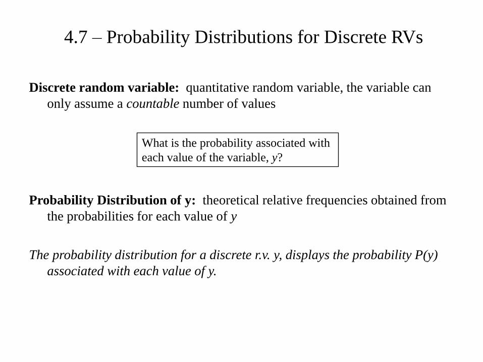
4.7 – Probability Distributions for Discrete RVs

Discrete random variable: quantitative random variable, the variable can

only assume a countable number of values

Probability Distribution of y: theoretical relative frequencies obtained from

the probabilities for each value of y

The probability distribution for a discrete r.v. y, displays the probability P(y)

associated with each value of y.

What is the probability associated with

each value of the variable, y?

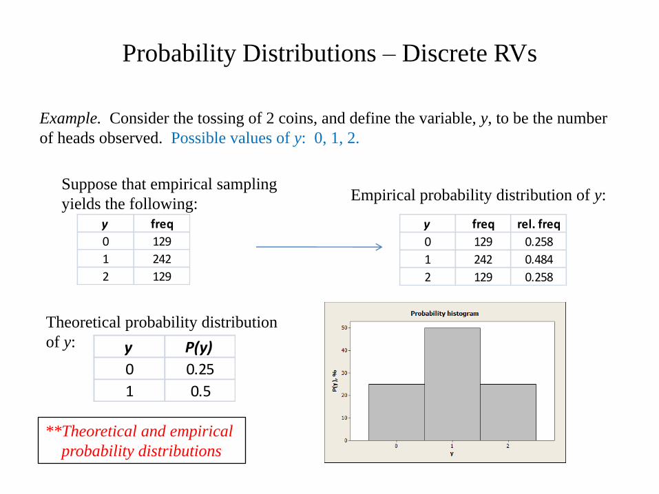
Probability Distributions – Discrete RVs

Example. Consider the tossing of 2 coins, and define the variable, y, to be the number

of heads observed. Possible values of y: 0, 1, 2.

y freq

0 129

1 242

2 129

Suppose that empirical sampling

yields the following:

y freq rel. freq

0 129 0.258

1 242 0.484

2 129 0.258

Empirical probability distribution of y:

y P(y)

0 0.25

1 0.5

Theoretical probability distribution

of y:

**Theoretical and empirical

probability distributions

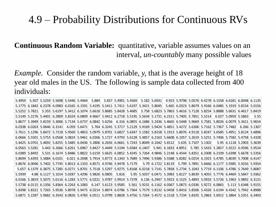
4.9 – Probability Distributions for Continuous RVs

Continuous Random Variable: quantitative, variable assumes values on an

interval, un-countably many possible values

Example. Consider the random variable, y, that is the average height of 18

year old males in the US. The following is sample data collected from 400

individuals:5.4959 5.507 5.5259 5.5698 5.5446 5.4464 5.884 5.837 5.4901 5.4569 5.182 5.6931 4.923 5.9798 5.0576 6.4278 6.1558 6.6181 6.0048 6.1135

5.1775 6.1842 6.2378 6.0983 6.0165 6.1591 5.4195 5.5411 5.7411 5.6197 5.3421 5.8045 5.665 6.0323 5.8679 5.9166 6.0485 5.1919 5.8154 5.0156

5.5252 5.7821 5.355 5.6197 5.3412 6.1074 5.6618 5.8685 5.8428 5.4685 5.758 5.6823 5.7863 5.4616 5.7128 5.8254 5.8888 5.6631 6.4617 5.8419

5.5149 5.2276 5.4401 6.2809 5.8324 6.0809 4.9667 5.9412 6.2718 5.5195 5.5634 5.1731 6.2311 5.7405 5.7851 5.5214 6.027 5.0959 5.5863 5.55

5.8677 5.3949 5.8159 5.3006 5.7134 5.6737 6.0842 5.6256 6.316 6.0855 6.1686 5.2436 5.4665 6.5448 5.9669 5.7581 5.8026 6.0079 5.3411 5.9654

6.0338 6.0263 5.0646 6.3141 6.059 5.6471 5.764 6.3245 5.3717 5.2129 5.9169 5.9424 5.4851 5.4272 5.6306 5.7162 5.7367 5.7482 6.266 5.1307

5.7611 5.1296 5.8472 5.7218 5.9569 5.4853 5.0979 5.8701 5.6827 5.6347 5.1582 5.8158 5.1913 5.8076 4.9118 5.8247 5.6585 5.4951 5.8124 5.6896

6.0666 5.5501 5.5753 6.0568 5.0824 5.9461 6.0266 5.1727 4.9793 5.6128 5.4857 6.2163 5.6608 6.1057 5.2619 5.5251 5.7406 5.7582 5.4758 5.4328

5.4425 6.0701 5.4692 5.8255 5.5485 6.0436 5.2806 6.2656 6.0661 5.7243 5.8049 6.1042 5.6512 5.635 5.7107 5.1302 5.95 6.1118 5.2903 5.3639

6.0563 5.5281 5.443 6.2666 5.6261 5.6967 5.8427 5.4449 5.5194 5.6584 6.1407 5.941 6.1833 4.8951 5.785 5.5433 5.2857 5.9222 6.0596 5.9524

6.0389 5.8492 5.531 6.1674 5.8486 5.8822 5.6159 5.6625 6.0852 5.4245 5.7264 4.9846 5.2148 6.4544 5.8351 6.3308 6.2109 5.6398 5.6678 5.5356

5.8694 5.6393 5.5884 6.0101 6.021 6.2048 5.7914 5.8772 6.1343 5.7689 5.7496 5.9386 5.5588 5.8282 6.0254 6.1923 5.4785 5.8039 5.7008 6.4147

5.8676 6.0046 5.7402 5.7745 5.8013 6.1333 4.8571 4.9746 5.9478 5.7179 5.79 6.1722 5.8119 5.799 5.7891 5.6666 6.1177 5.9385 5.5016 5.9354

5.657 6.1379 6.3875 5.7285 6.0271 5.8701 5.7518 5.5297 5.9275 5.8168 6.0218 5.7141 5.7858 5.2734 5.1043 5.7719 6.1106 5.4786 5.7649 5.8087

5.5939 4.88 6.1127 5.1014 5.0287 5.4296 5.9826 6.0805 5.816 5.95 5.5037 6.0471 5.3983 5.8127 5.8639 5.4055 5.7776 6.4469 5.5847 5.9362

6.0166 5.3819 5.5075 5.6116 6.1283 5.5771 6.0221 5.9787 5.9914 5.7378 6.136 6.2947 5.5923 6.1525 5.4893 5.0933 5.5726 5.1963 5.9892 6.3131

5.5738 6.0115 6.1356 5.8364 6.2263 6.1083 6.147 5.6123 5.9585 5.561 5.9231 6.1162 6.0367 5.0873 6.0336 5.9272 6.0865 5.113 5.6348 5.9155

5.8398 5.8321 5.7265 5.9536 5.8978 5.9475 6.0214 5.8874 6.0786 5.7364 5.7579 5.8132 6.0458 5.8416 5.8506 5.4326 5.6194 6.4342 5.7942 4.8988

5.6871 5.2287 5.9682 6.3543 6.0826 5.4783 6.0511 5.0799 5.8828 5.4756 5.7264 5.4572 6.1518 5.7234 5.8335 5.2863 5.6912 5.3864 5.5351 6.3403

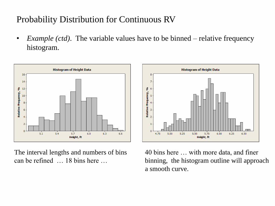
Probability Distribution for Continuous RV

• Example (ctd). The variable values have to be binned – relative frequency

histogram.

The interval lengths and numbers of bins

can be refined … 18 bins here …

40 bins here … with more data, and finer

binning, the histogram outline will approach

a smooth curve.

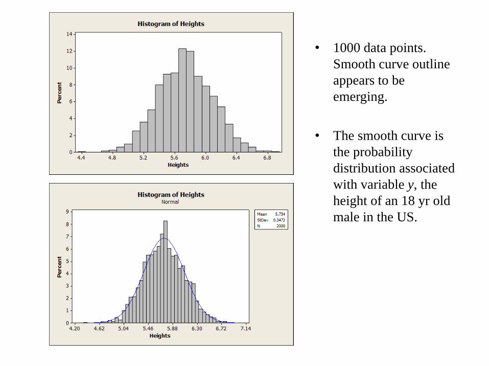
• 1000 data points.

Smooth curve outline

appears to be

emerging.

• The smooth curve is

the probability

distribution associated

with variable y, the

height of an 18 yr old

male in the US.

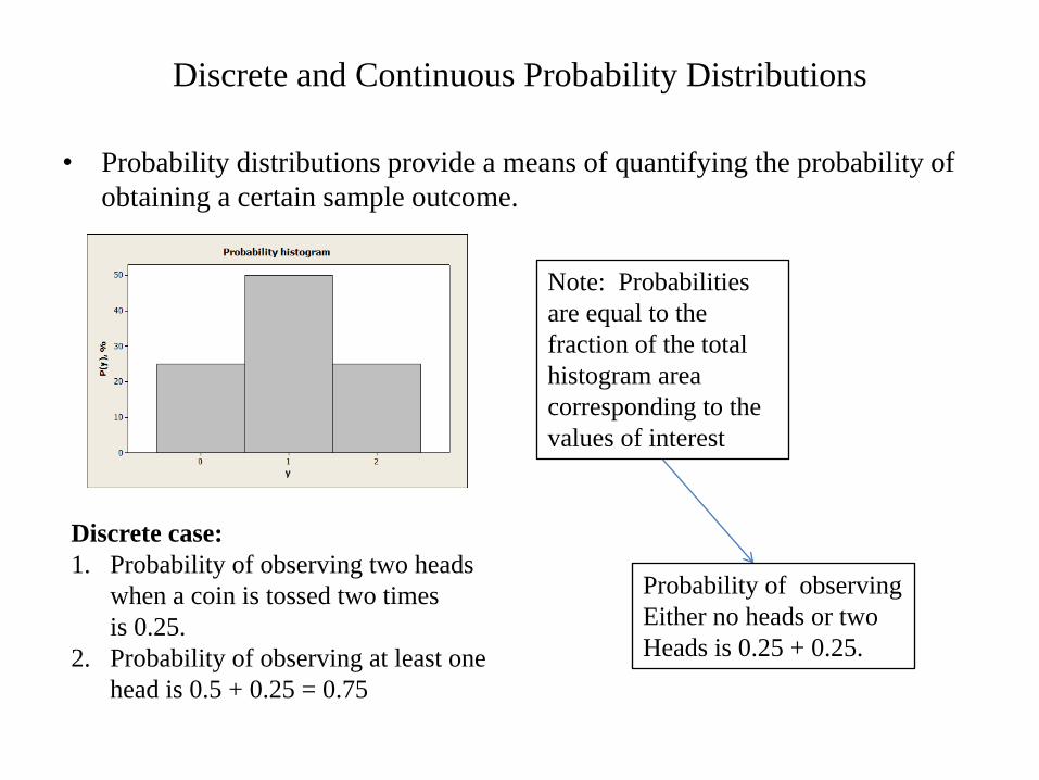
Discrete and Continuous Probability Distributions

• Probability distributions provide a means of quantifying the probability of

obtaining a certain sample outcome.

Discrete case:

1. Probability of observing two heads

when a coin is tossed two times

is 0.25.

2. Probability of observing at least one

head is 0.5 + 0.25 = 0.75

Note: Probabilities

are equal to the

fraction of the total

histogram area

corresponding to the

values of interest

Probability of observing

Either no heads or two

Heads is 0.25 + 0.25.

Discrete and Continuous Probability Distributions

Continuous case:

1. Does it make sense to ask “what is the

probability

that an 18 y.o. male is 5’10”?” NO

2. Note: The distribution plot was created using

relative frequencies – total area under the plot

is 1.

3. We compute the probability of a value falling

in a certain range of values, by computing the

area that lies under the distribution plot, over

that range.

The probability that an 18 y.o.

male has a height that lies between

5.7 and 5.8 feet is approx 0.1.

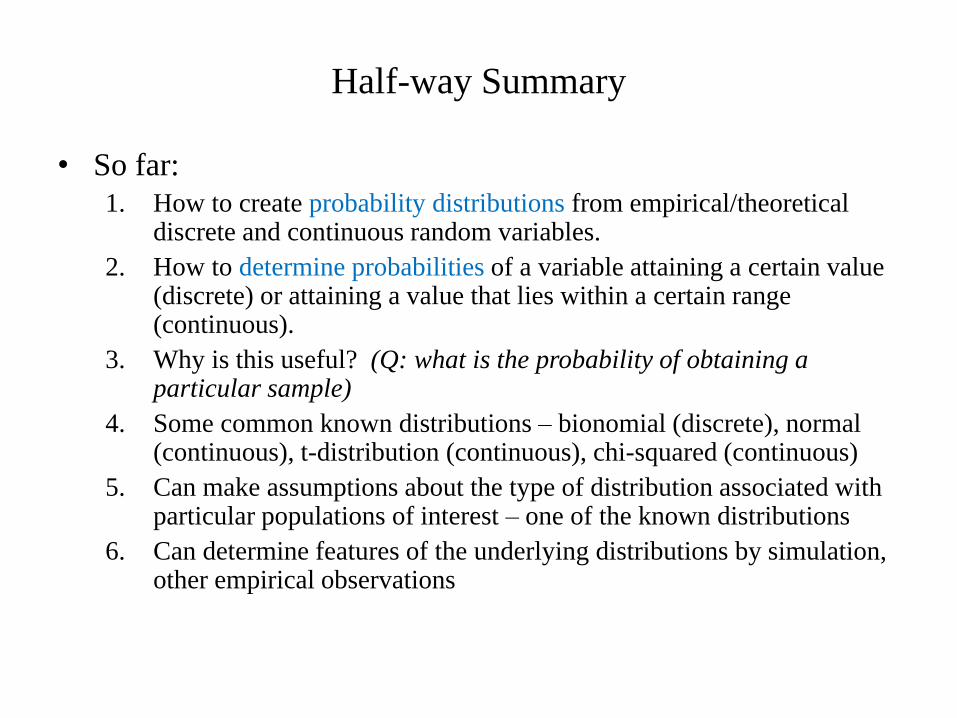
Half-way Summary

• So far:

1. How to create probability distributions from empirical/theoretical discrete and continuous random variables.

2. How to determine probabilities of a variable attaining a certain value (discrete) or attaining a value that lies within a certain range (continuous).

3. Why is this useful? (Q: what is the probability of obtaining a particular sample)

4. Some common known distributions – bionomial (discrete), normal (continuous), t-distribution (continuous), chi-squared (continuous)

5. Can make assumptions about the type of distribution associated with particular populations of interest – one of the known distributions

6. Can determine features of the underlying distributions by simulation, other empirical observations

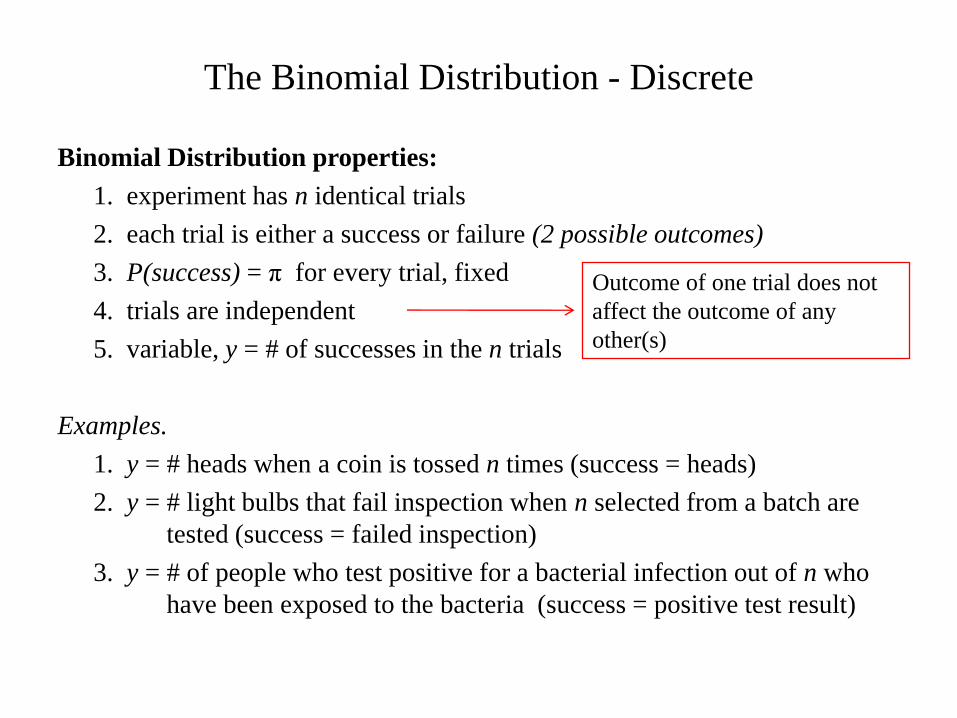
The Binomial Distribution - Discrete

Binomial Distribution properties:

1. experiment has n identical trials

2. each trial is either a success or failure (2 possible outcomes)

3. P(success) = π for every trial, fixed

4. trials are independent

5. variable, y = # of successes in the n trials

Examples.

1. y = # heads when a coin is tossed n times (success = heads)

2. y = # light bulbs that fail inspection when n selected from a batch are

tested (success = failed inspection)

3. y = # of people who test positive for a bacterial infection out of n who

have been exposed to the bacteria (success = positive test result)

Outcome of one trial does not

affect the outcome of any

other(s)

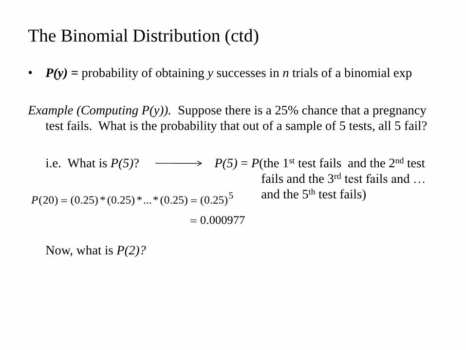
• P(y) = probability of obtaining y successes in n trials of a binomial exp

Example (Computing P(y)). Suppose there is a 25% chance that a pregnancy

test fails. What is the probability that out of a sample of 5 tests, all 5 fail?

i.e. What is P(5)? P(5) = P(the 1st test fails and the 2nd test

fails and the 3rd test fails and …

and the 5th test fails)

Now, what is P(2)?

The Binomial Distribution (ctd)

5)25.0()25.0(*...*)25.0(*)25.0()20( P

000977.0

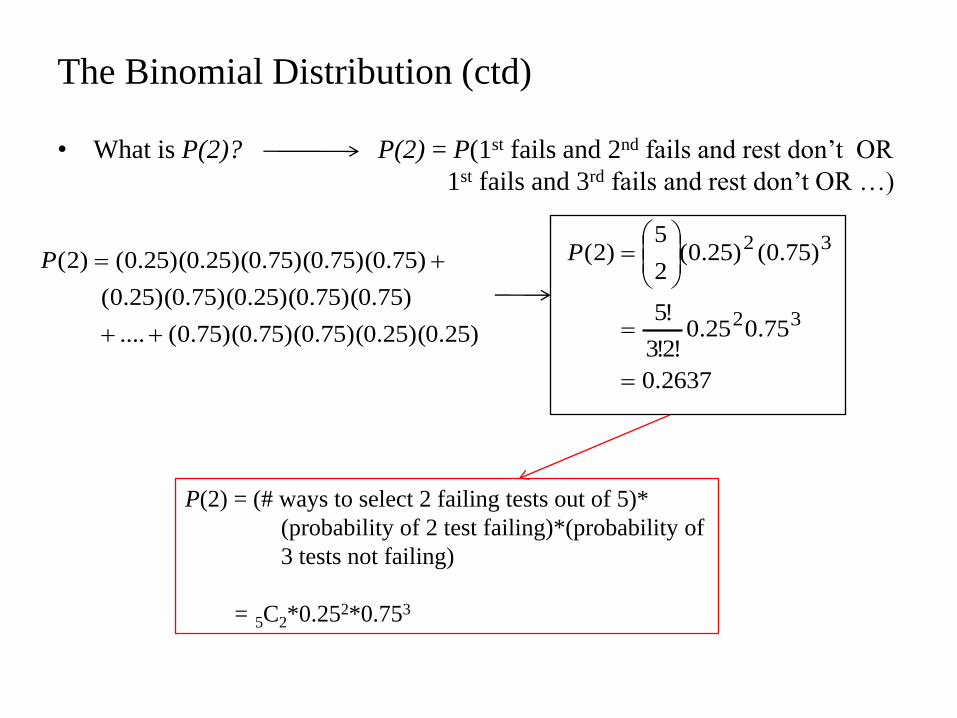
• What is P(2)? P(2) = P(1st fails and 2nd fails and rest don’t OR

1st fails and 3rd fails and rest don’t OR …)

)25.0)(25.0)(75.0)(75.0)(75.0(....

)75.0)(75.0)(25.0)(75.0)(25.0(

)75.0)(75.0)(75.0)(25.0)(25.0()2(

P

2637.0

75.025.0!2!3

!5

)75.0()25.0(2

5)2(

32

32

P

The Binomial Distribution (ctd)

P(2) = (# ways to select 2 failing tests out of 5)*

(probability of 2 test failing)*(probability of

3 tests not failing)

= 5C2*0.252*0.753

The Binomial Distribution (ctd)

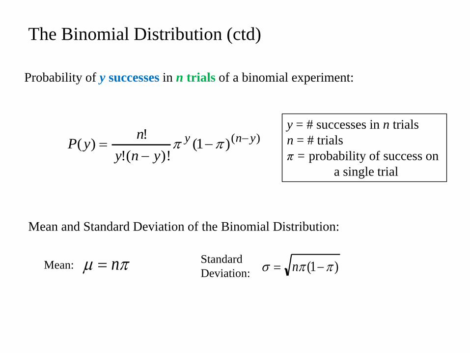
)()1(

)!(!

!)(

yny

yny

nyP

Probability of y successes in n trials of a binomial experiment:

y = # successes in n trials

n = # trials

π = probability of success on

a single trial

Mean and Standard Deviation of the Binomial Distribution:

n )1( nMean:Standard

Deviation:

• Example. What is the probability that 6 out of 20 tests fail, if the

probability that any one test fails is 25%? Success = test fails

So, π = 0.25, n = 20, y = 6

1686.0

75.025.01*2*3*4*5*6

15*16*17*18*19*20

75.025.0!14!6

!20)6(

146

146

P

Note: P(y ≥ 7) = P(7) + P(8) + P(9) + … + P(20)

= 1 – P(y ≤ 6)

• What are the mean and deviation of this distribution?

5

25.0*20

94.1

)75.0(25.0*20

The Binomial Distribution (ctd)

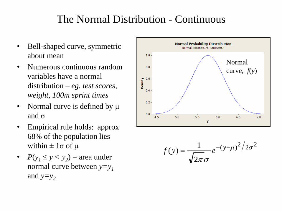
• Bell-shaped curve, symmetric

about mean

• Numerous continuous random

variables have a normal

distribution – eg. test scores,

weight, 100m sprint times

• Normal curve is defined by μ

and σ

• Empirical rule holds: approx

68% of the population lies

within ± 1σ of μ

• P(y1 ≤ y < y2) = area under

normal curve between y=y1

and y=y2

The Normal Distribution - Continuous

Normal

curve, f(y)

222)(

2

1)(

yeyf

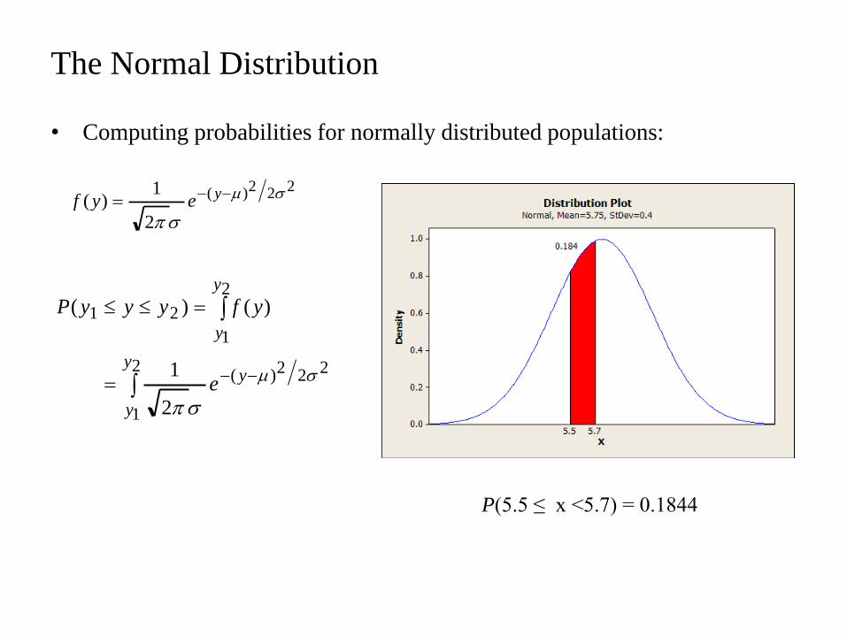
• Computing probabilities for normally distributed populations:

The Normal Distribution

222)(

2

1)(

yeyf

2

1

222)(

2

1

21

2

1

)()(

y

y

y

y

y

e

yfyyyP

P(5.5 ≤ x <5.7) = 0.1844

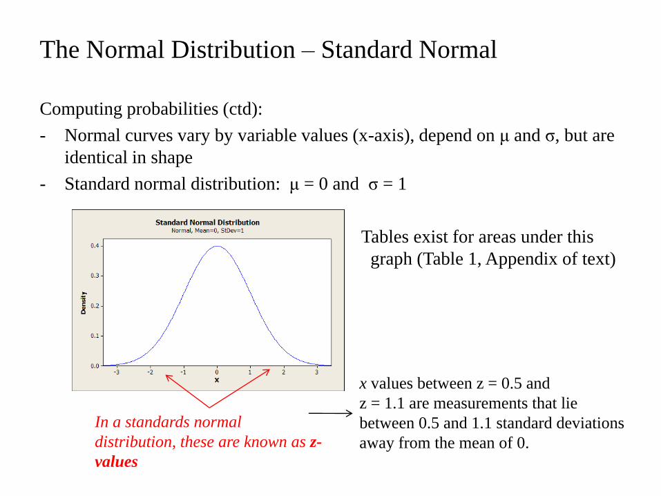
Computing probabilities (ctd):

- Normal curves vary by variable values (x-axis), depend on μ and σ, but are

identical in shape

- Standard normal distribution: μ = 0 and σ = 1

- Tables exist for areas under this

graph (Table 1, Appendix of text)

-

The Normal Distribution – Standard Normal

In a standards normal

distribution, these are known as z-

values

x values between z = 0.5 and

z = 1.1 are measurements that lie

between 0.5 and 1.1 standard deviations

away from the mean of 0.

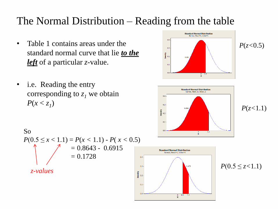
• Table 1 contains areas under the

standard normal curve that lie to the

left of a particular z-value.

• i.e. Reading the entry

corresponding to z1 we obtain

P(x < z1)

The Normal Distribution – Reading from the table

So

P(0.5 ≤ x < 1.1) = P(x < 1.1) - P( x < 0.5)

= 0.8643 - 0.6915

= 0.1728

z-values

P(z<0.5)

P(z<1.1)

P(0.5 ≤ z<1.1)

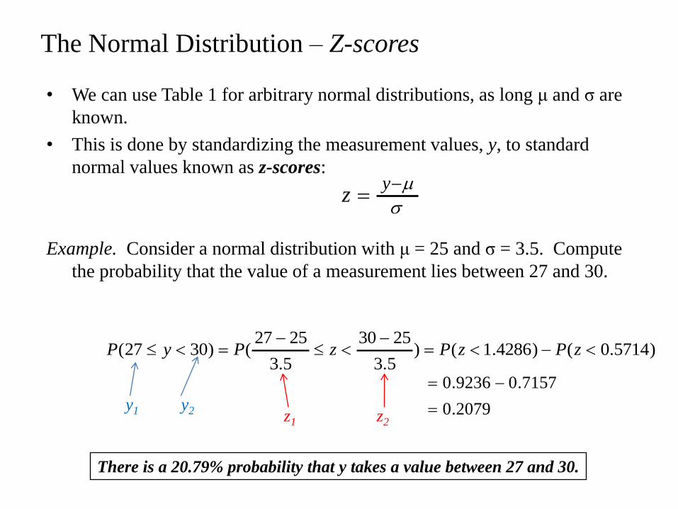
• We can use Table 1 for arbitrary normal distributions, as long μ and σ are

known.

• This is done by standardizing the measurement values, y, to standard

normal values known as z-scores:

Example. Consider a normal distribution with μ = 25 and σ = 3.5. Compute

the probability that the value of a measurement lies between 27 and 30.

The Normal Distribution – Z-scores

yz

)5714.0()4286.1()5.3

2530

5.3

2527()3027(

zPzPzPyP

y1 y2 z1 z22079.0

7157.09236.0

There is a 20.79% probability that y takes a value between 27 and 30.

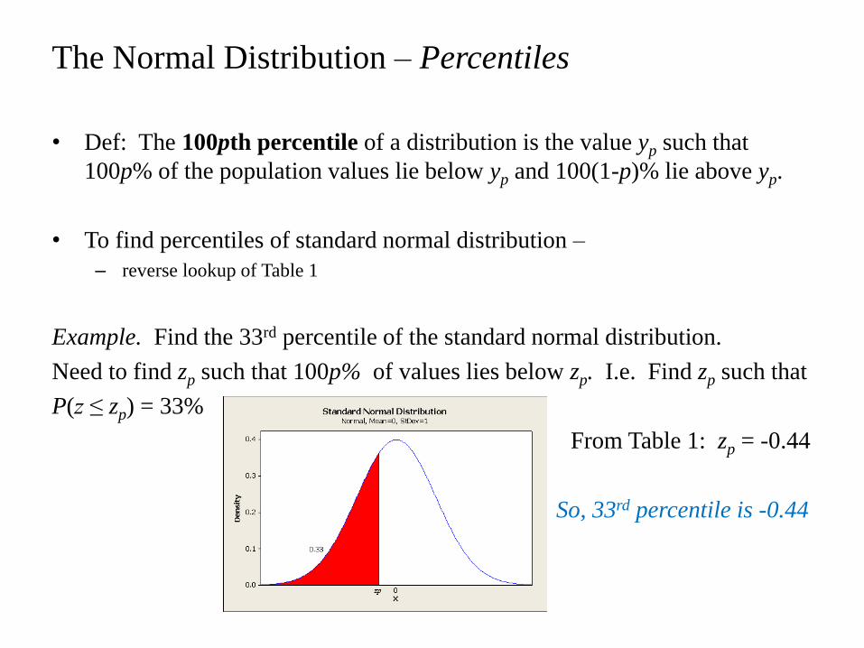
• Def: The 100pth percentile of a distribution is the value yp such that

100p% of the population values lie below yp and 100(1-p)% lie above yp.

• To find percentiles of standard normal distribution –

– reverse lookup of Table 1

Example. Find the 33rd percentile of the standard normal distribution.

Need to find zp such that 100p% of values lies below zp. I.e. Find zp such that

P(z ≤ zp) = 33%

From Table 1: zp = -0.44

So, 33rd percentile is -0.44

The Normal Distribution – Percentiles

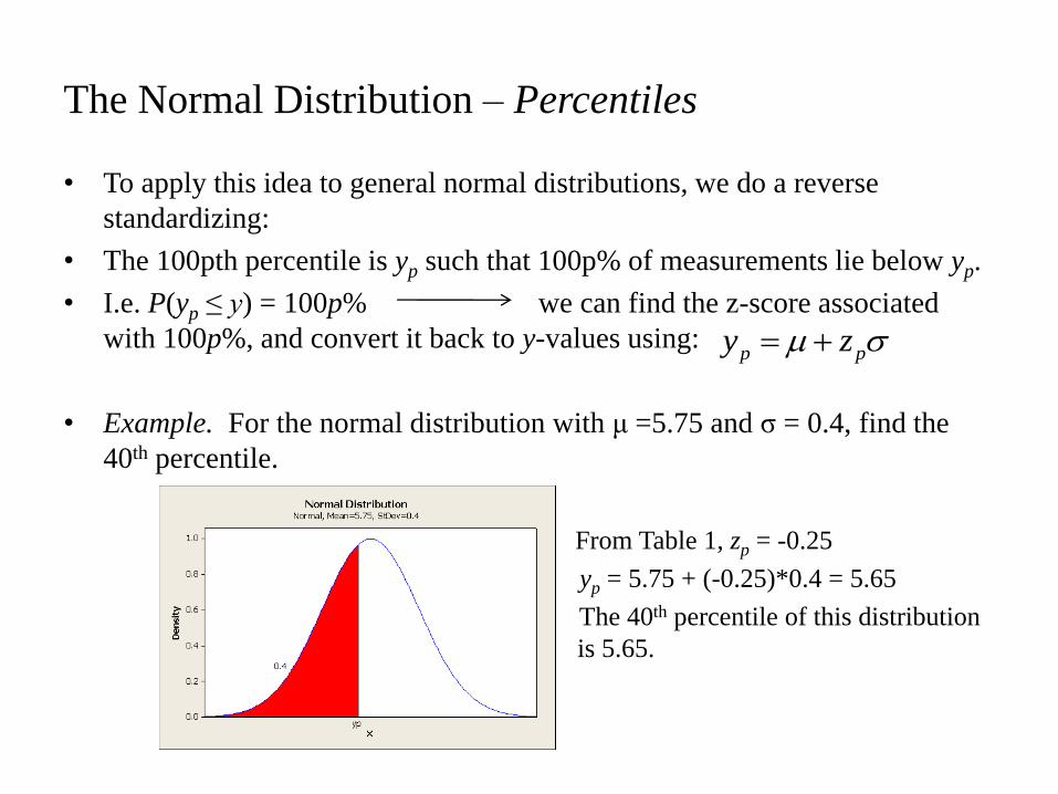
• To apply this idea to general normal distributions, we do a reverse

standardizing:

• The 100pth percentile is yp such that 100p% of measurements lie below yp.

• I.e. P(yp ≤ y) = 100p% we can find the z-score associated

with 100p%, and convert it back to y-values using:

• Example. For the normal distribution with μ =5.75 and σ = 0.4, find the

40th percentile.

• From Table 1, zp = -0.25

• yp = 5.75 + (-0.25)*0.4 = 5.65

• The 40th percentile of this distribution

is is 5.65.

The Normal Distribution – Percentiles

pp zy