Embed Size (px)
Citation preview
Chapter 4
Continuous Random Variables and Probability Distributions
PROBABILITY (6MTCOAE205)
Ch. 4-1
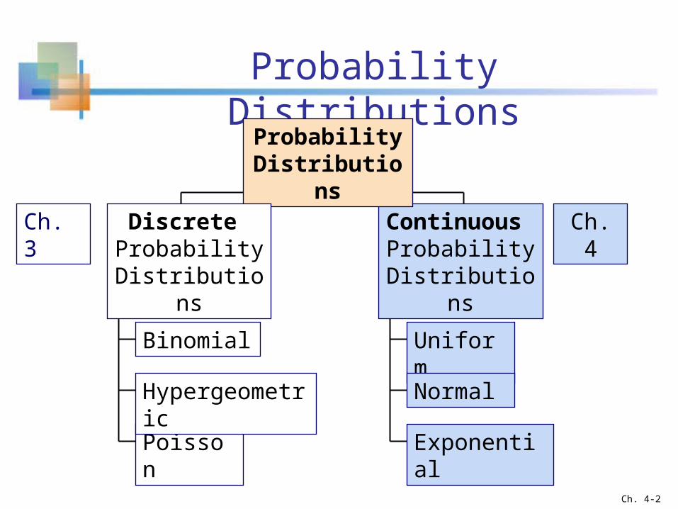
Probability Distributions
Continuous Probability
Distributions
Binomial
Poisson
Hypergeometric
Probability Distributions
Discrete Probability
Distributions
Uniform
Normal
Exponential
Ch. 3 Ch. 4
Ch. 4-2
Continuous Probability Distributions
A continuous random variable is a variable that can assume any value in an interval thickness of an item time required to complete a task temperature of a solution height, in inches
These can potentially take on any value, depending only on the ability to measure accurately.
Ch. 4-3
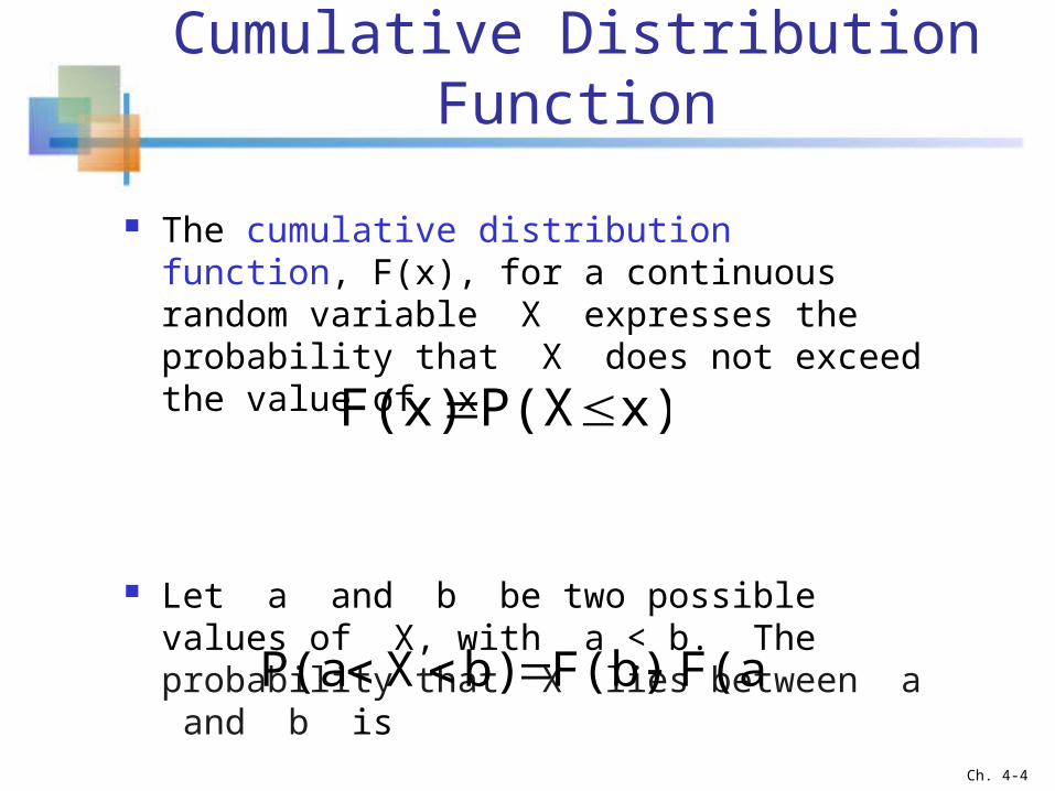
Cumulative Distribution Function
The cumulative distribution function, F(x), for a continuous random variable X expresses the probability that X does not exceed the value of x
Let a and b be two possible values of X, with a < b. The probability that X lies between a and b is
x)P(XF(x)
F(a)F(b)b)XP(a
Ch. 4-4
Probability Density Function
The probability density function, f(x), of random variable X has the following properties:
1. f(x) > 0 for all values of x
2. The area under the probability density function f(x) over all values of the random variable X is equal to 1.0
3. The probability that X lies between two values is the area under the density function graph between the two values
Ch. 4-5
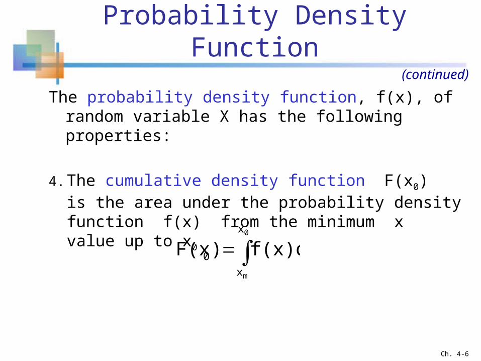
Probability Density Function
The probability density function, f(x), of random variable X has the following properties:
4. The cumulative density function F(x0) is the area under the probability density function f(x) from the minimum x value up to x0
where xm is the minimum value of the random variable x
0
m
x
x
0 f(x)dx)F(x
Ch. 4-6
(continued)
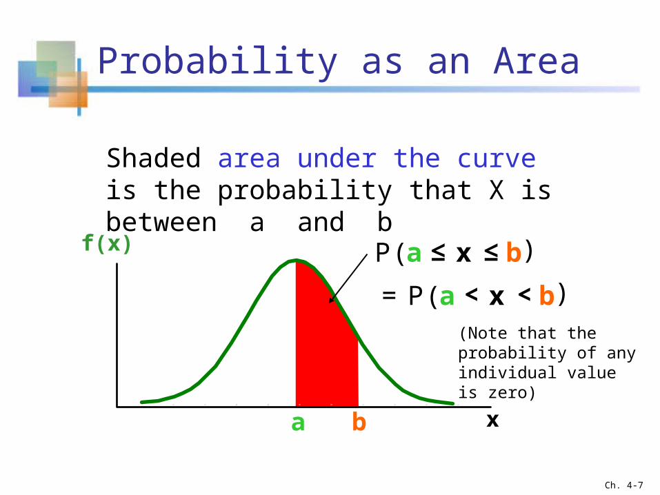
Probability as an Area
a b x
f(x) P a x b( )≤
Shaded area under the curve is the probability that X is between a and b
≤
P a x b( )<<=(Note that the probability of any individual value is zero)
Ch. 4-7
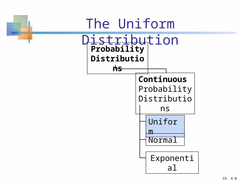
The Uniform Distribution
Probability Distributions
Uniform
Normal
Exponential
Continuous Probability
Distributions
Ch. 4-8
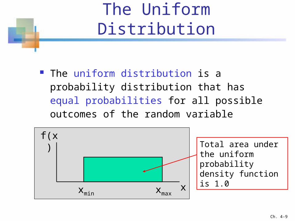
The Uniform Distribution
The uniform distribution is a probability distribution that has equal probabilities for all possible outcomes of the random variable
xmin xmaxx
f(x)Total area under the uniform probability density function is 1.0
Ch. 4-9
The Uniform Distribution
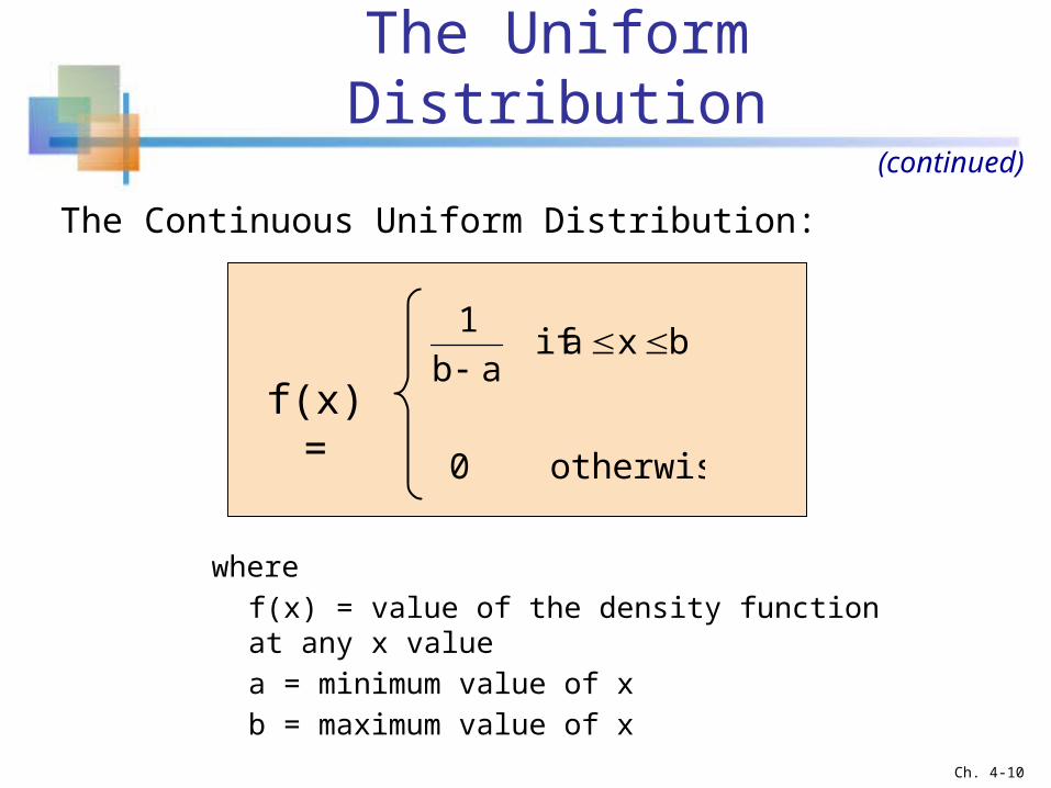
The Continuous Uniform Distribution:
otherwise 0
bxaifab
1
where
f(x) = value of the density function at any x value
a = minimum value of x
b = maximum value of x
(continued)
f(x) =
Ch. 4-10
Properties of the Uniform Distribution
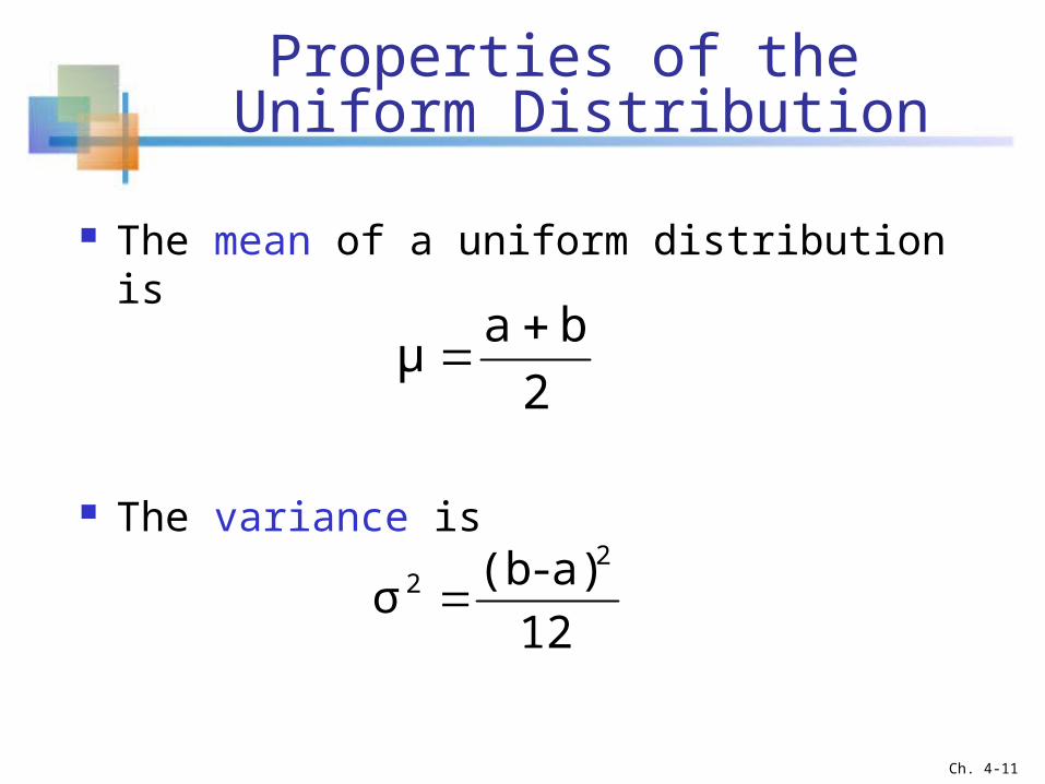
The mean of a uniform distribution is
The variance is
2
baμ
12
a)-(bσ
22
Ch. 4-11
Uniform Distribution Example
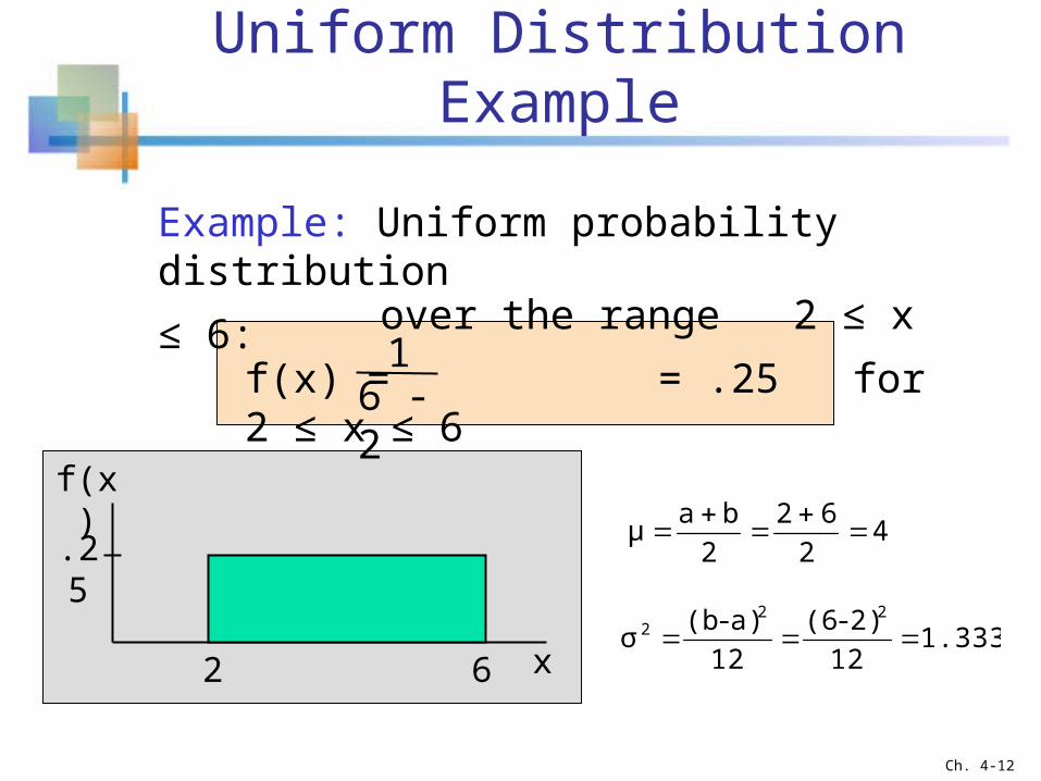
Example: Uniform probability distribution over the range 2 ≤ x ≤ 6:
2 6
.25
f(x) = = .25 for 2 ≤ x ≤ 66 - 21
x
f(x)
42
62
2
baμ
1.33312
2)-(6
12
a)-(bσ
222
Ch. 4-12
Expectations for Continuous Random Variables
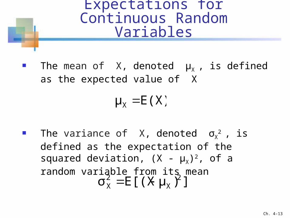
The mean of X, denoted μX , is defined as the expected value of X
The variance of X, denoted σX2 , is defined as the
expectation of the squared deviation, (X - μX)2, of a random variable from its mean
E(X)μX
])μE[(Xσ 2X
2X
Ch. 4-13
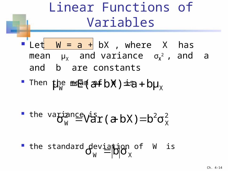
Linear Functions of Variables
Let W = a + bX , where X has mean μX and variance σX
2 , and a and b are constants
Then the mean of W is
the variance is
the standard deviation of W is
XW bμabX)E(aμ
2X
22W σbbX)Var(aσ
XW σbσ Ch. 4-14
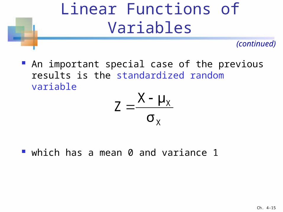
Linear Functions of Variables
An important special case of the previous results is the standardized random variable
which has a mean 0 and variance 1
(continued)
X
X
σ
μXZ
Ch. 4-15
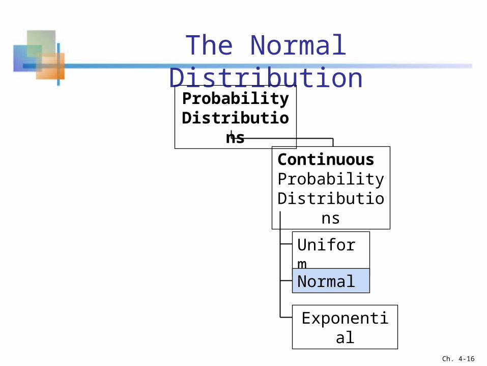
The Normal Distribution
Continuous Probability
Distributions
Probability Distributions
Uniform
Normal
Exponential
Ch. 4-16
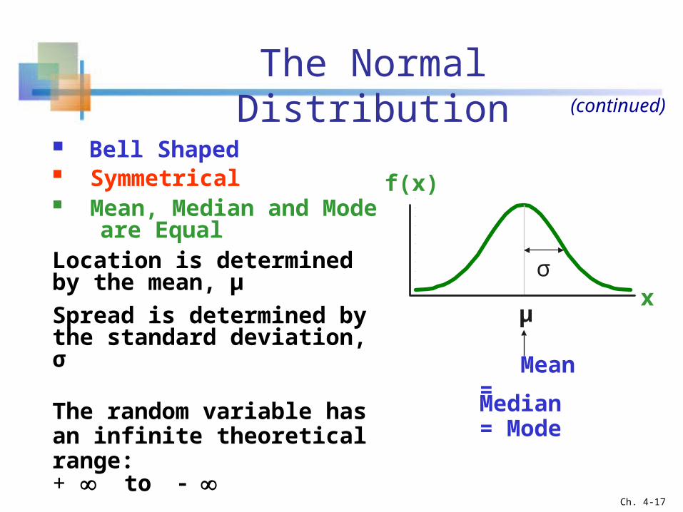
‘Bell Shaped’ Symmetrical Mean, Median and Mode
are EqualLocation is determined by the mean, μ
Spread is determined by the standard deviation, σ
The random variable has an infinite theoretical range: + to
Mean = Median = Mode
x
f(x)
μ
σ
(continued)
Ch. 4-17
The Normal Distribution
The normal distribution closely approximates the probability distributions of a wide range of random variables
Distributions of sample means approach a normal distribution given a “large” sample size
Computations of probabilities are direct and elegant
The normal probability distribution has led to good business decisions for a number of applications
(continued)
Ch. 4-18
The Normal Distribution
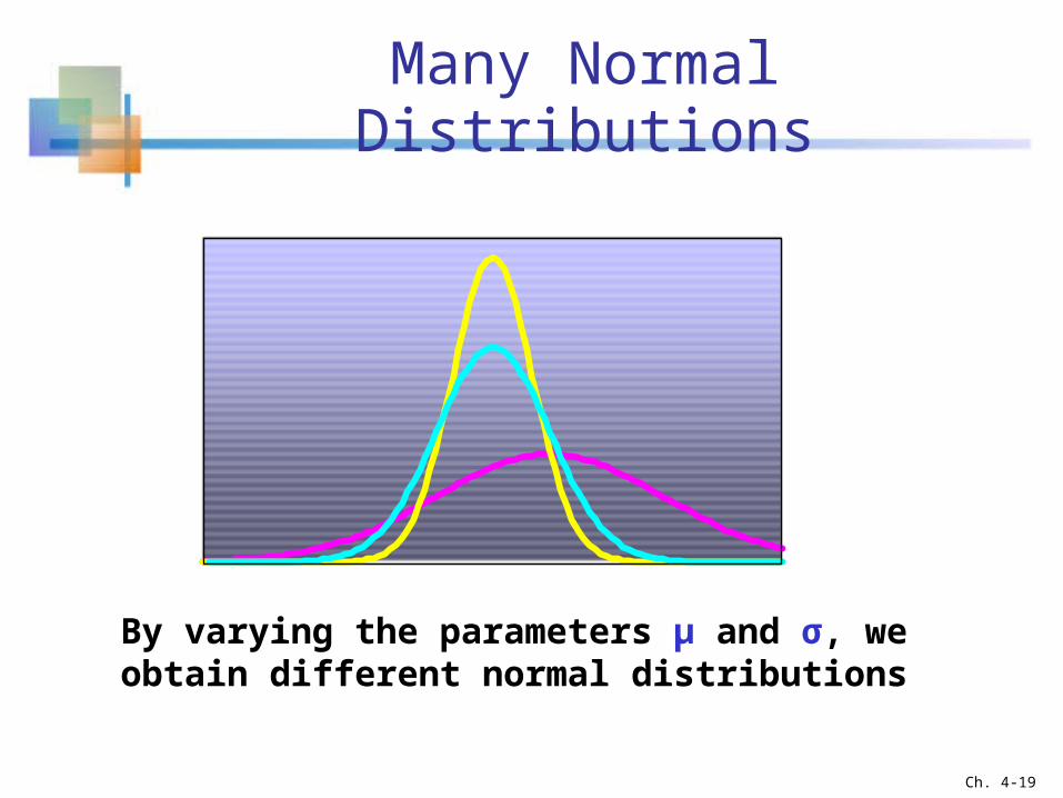
By varying the parameters μ and σ, we obtain different normal distributions
Many Normal Distributions
Ch. 4-19
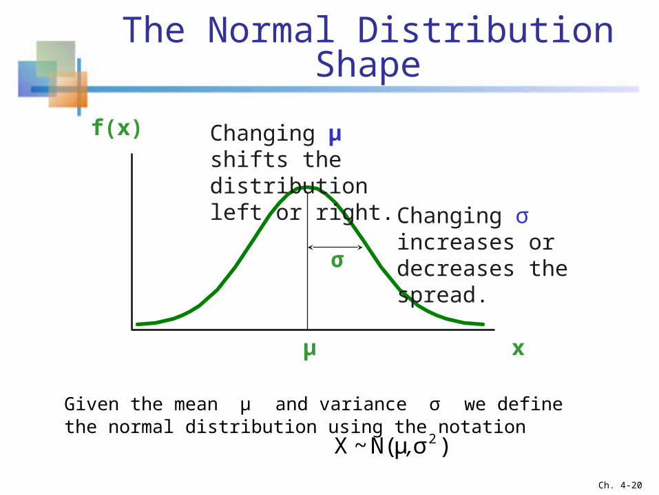
The Normal Distribution Shape
x
f(x)
μ
σ
Changing μ shifts the distribution left or right.
Changing σ increases or decreases the spread.
Given the mean μ and variance σ we define the normal distribution using the notation
)σN(μ~X 2,
Ch. 4-20
The Normal Probability Density Function
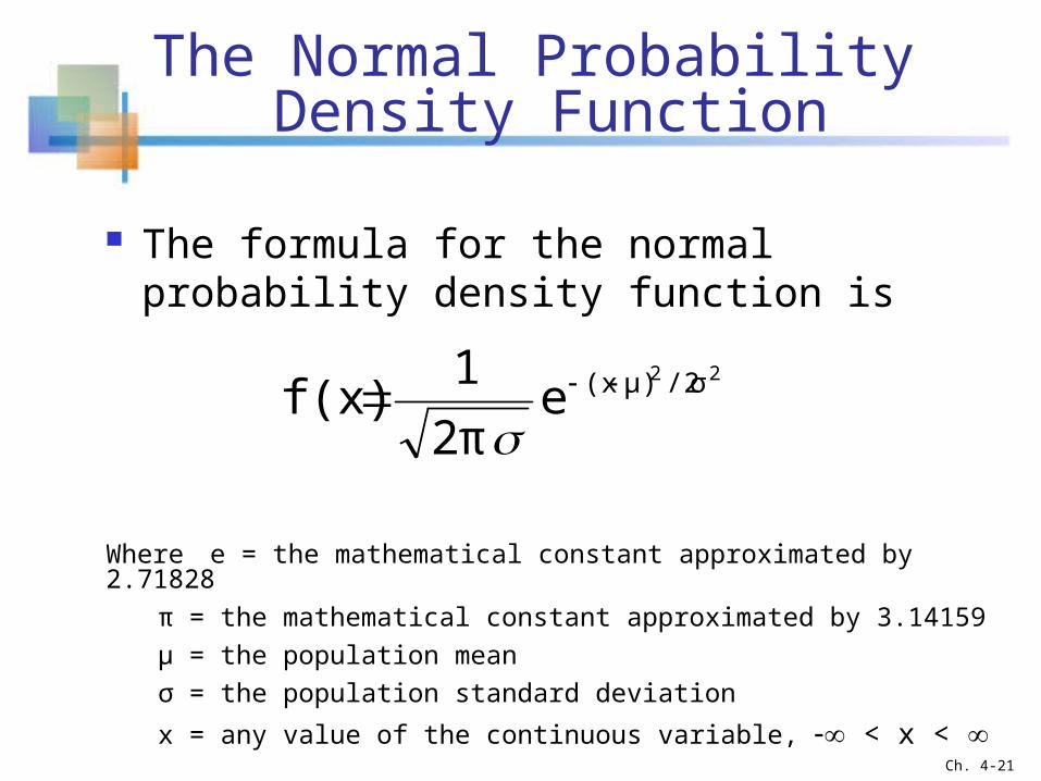
The formula for the normal probability density function is
Where e = the mathematical constant approximated by 2.71828
π = the mathematical constant approximated by 3.14159
μ = the population mean
σ = the population standard deviation
x = any value of the continuous variable, < x <
22 /2σμ)(xe2π
1f(x)
Ch. 4-21
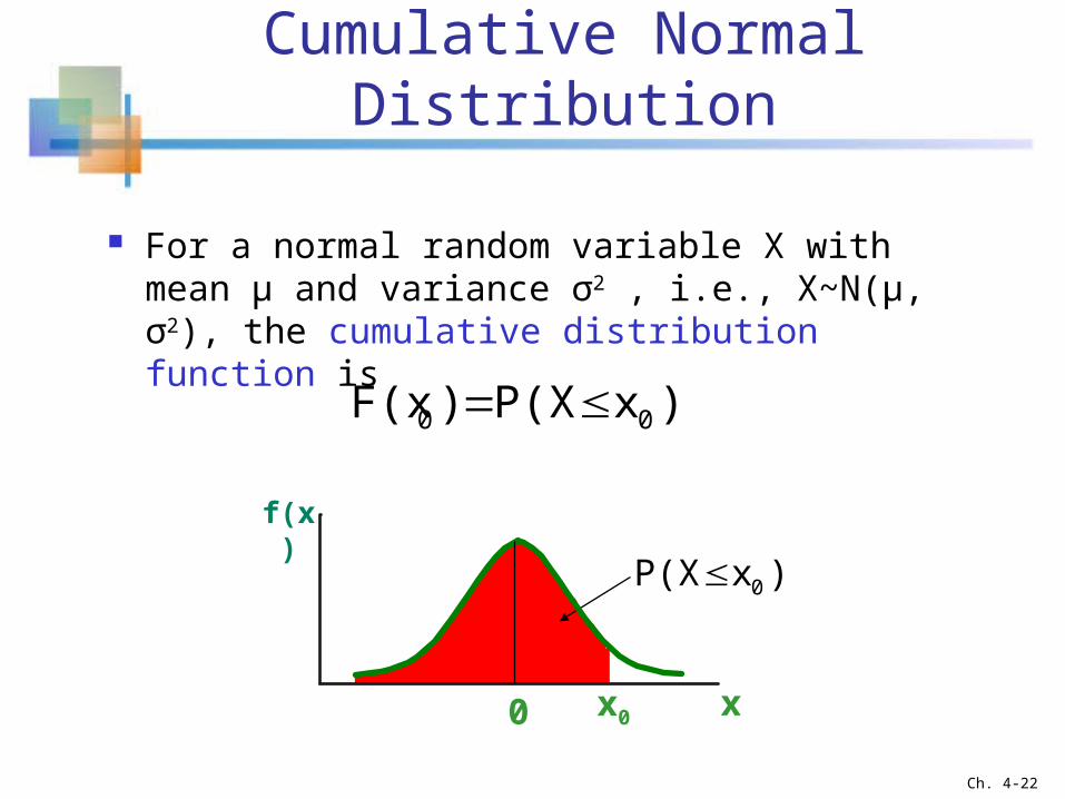
Cumulative Normal Distribution
For a normal random variable X with mean μ and variance σ2 , i.e., X~N(μ, σ2), the cumulative distribution function is
)xP(X)F(x 00
x0 x0
)xP(X 0
f(x)
Ch. 4-22
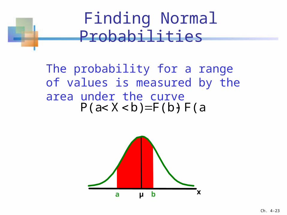
Finding Normal Probabilities
xbμa
The probability for a range of values is measured by the area under the curve
F(a)F(b)b)XP(a
Ch. 4-23
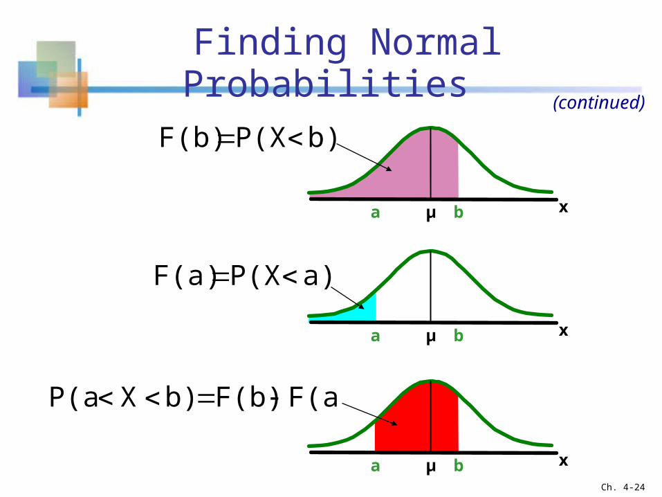
Finding Normal Probabilities
xbμa
xbμa
xbμa
(continued)
F(a)F(b)b)XP(a
a)P(XF(a)
b)P(XF(b)
Ch. 4-24
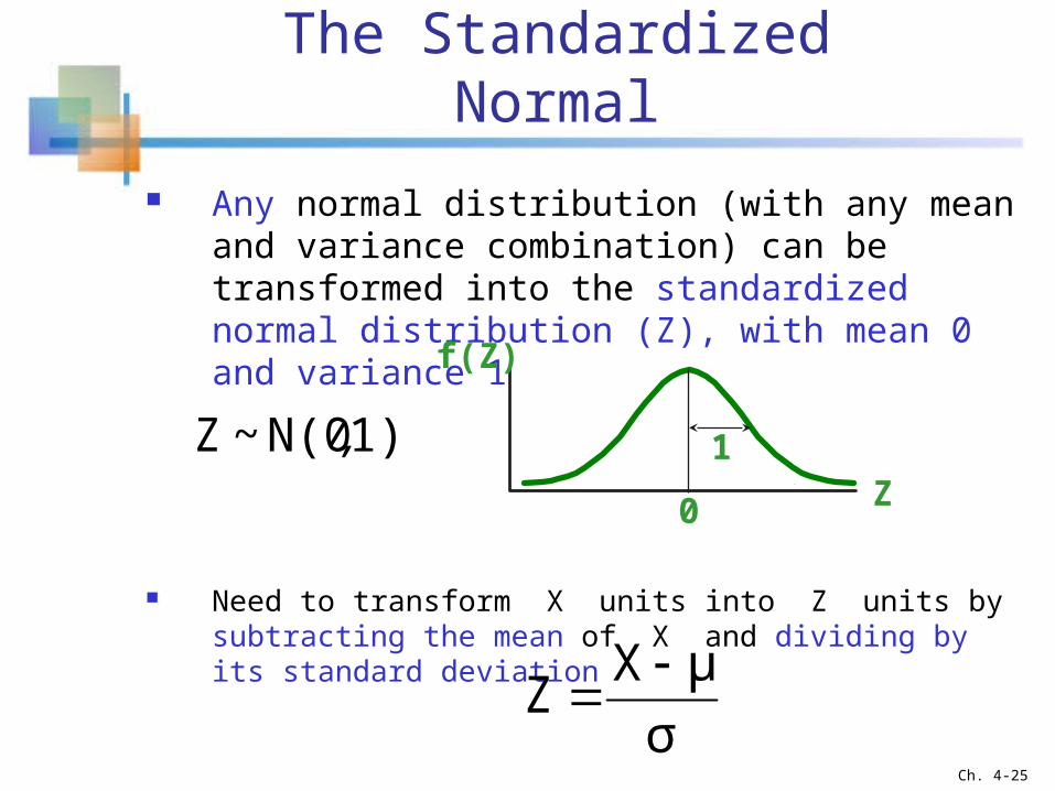
The Standardized Normal
Any normal distribution (with any mean and variance combination) can be transformed into the standardized normal distribution (Z), with mean 0 and variance 1
Need to transform X units into Z units by subtracting the mean of X and dividing by its standard deviation
1)N(0~Z ,
σ
μXZ
Z
f(Z)
0
1
Ch. 4-25
Example
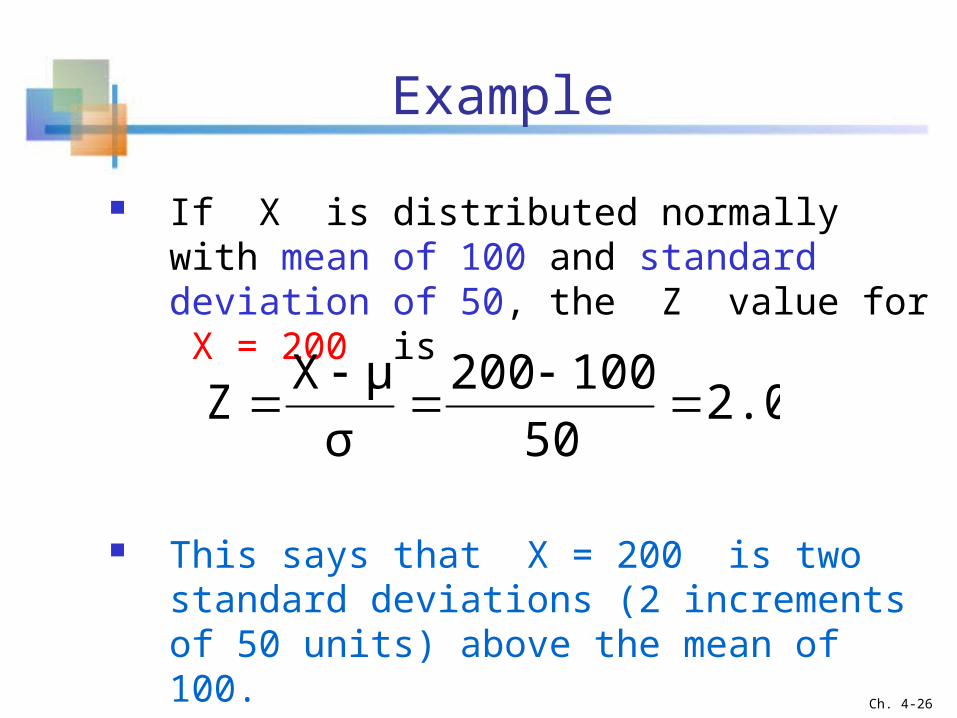
If X is distributed normally with mean of 100 and standard deviation of 50, the Z value for X = 200 is
This says that X = 200 is two standard deviations (2 increments of 50 units) above the mean of 100.
2.050
100200
σ
μXZ
Ch. 4-26
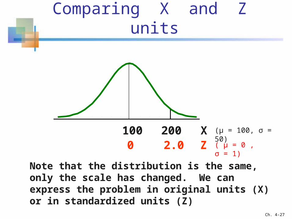
Comparing X and Z units
Z100
2.00200 X
Note that the distribution is the same, only the scale has changed. We can express the problem in original units (X) or in standardized units (Z)
(μ = 100, σ = 50)
( μ = 0 , σ = 1)
Ch. 4-27
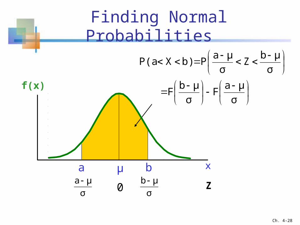
Finding Normal Probabilities
σ
μaF
σ
μbF
σ
μbZ
σ
μaPb)XP(a
a b x
f(x)
σ
μb σ
μa Z
µ
0
Ch. 4-28
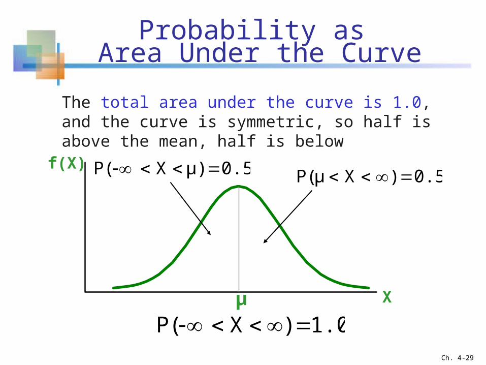
Probability as Area Under the Curve
f(X)
Xμ
0.50.5
The total area under the curve is 1.0, and the curve is symmetric, so half is above the mean, half is below
1.0)XP(
0.5)XP(μ 0.5μ)XP(
Ch. 4-29
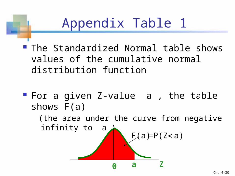
Appendix Table 1
The Standardized Normal table shows values of the cumulative normal distribution function
For a given Z-value a , the table shows F(a) (the area under the curve from negative infinity to a )
Z0 a
a)P(Z F(a)
Ch. 4-30
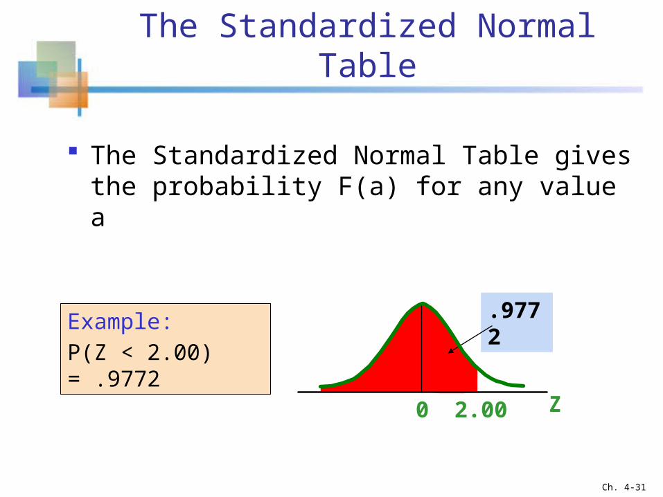
The Standardized Normal Table
Z0 2.00
.9772Example:
P(Z < 2.00) = .9772
The Standardized Normal Table gives the probability F(a) for any value a
Ch. 4-31
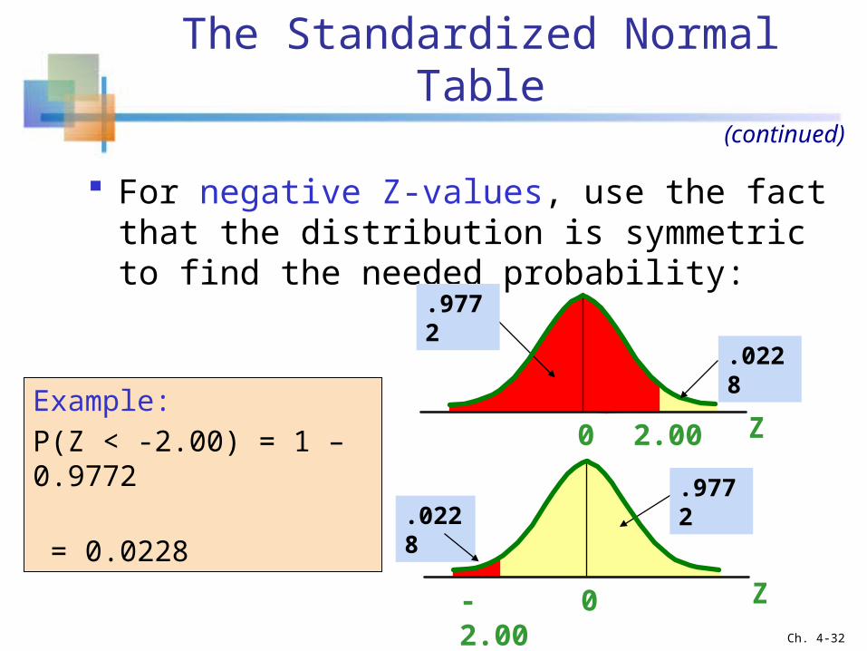
Z0-2.00
Example:
P(Z < -2.00) = 1 – 0.9772
= 0.0228
For negative Z-values, use the fact that the distribution is symmetric to find the needed probability:
Z0 2.00
.9772
.0228
.9772.0228
(continued)
Ch. 4-32
The Standardized Normal Table
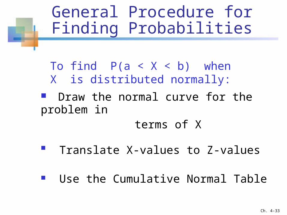
General Procedure for Finding Probabilities
Draw the normal curve for the problem in terms of X
Translate X-values to Z-values
Use the Cumulative Normal Table
To find P(a < X < b) when X is distributed normally:
Ch. 4-33
Finding Normal Probabilities
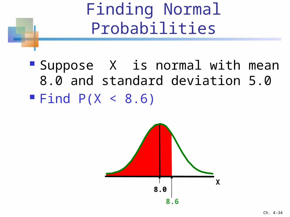
Suppose X is normal with mean 8.0 and standard deviation 5.0
Find P(X < 8.6)
X
8.6
8.0
Ch. 4-34
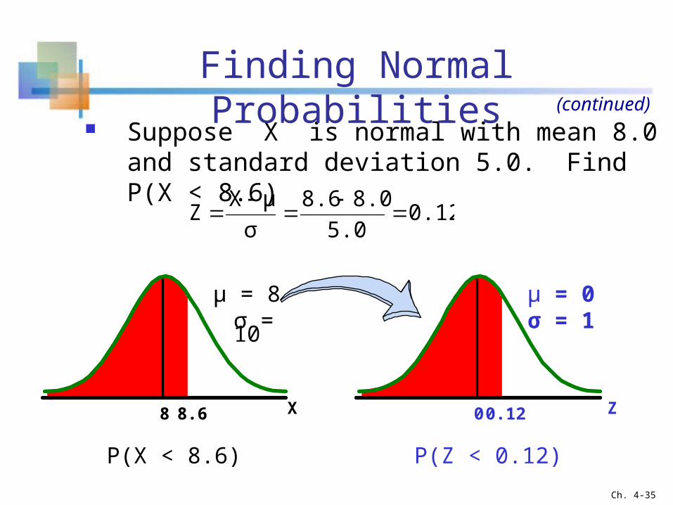
Suppose X is normal with mean 8.0 and standard deviation 5.0. Find P(X < 8.6)
Z0.12 0X8.6 8
μ = 8 σ = 10
μ = 0σ = 1
(continued)
0.125.0
8.08.6
σ
μXZ
P(X < 8.6) P(Z < 0.12)
Ch. 4-35
Finding Normal Probabilities
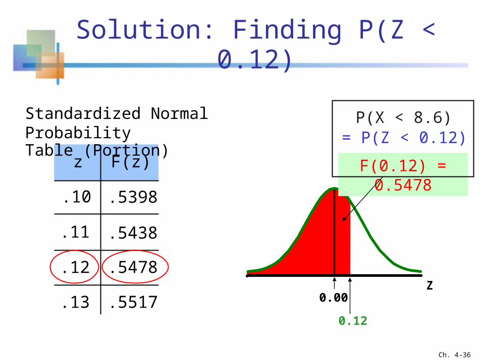
Solution: Finding P(Z < 0.12)
Z
0.12
z F(z)
.10 .5398
.11 .5438
.12 .5478
.13 .5517
F(0.12) = 0.5478
Standardized Normal Probability Table (Portion)
0.00
= P(Z < 0.12)P(X < 8.6)
Ch. 4-36
Upper Tail Probabilities
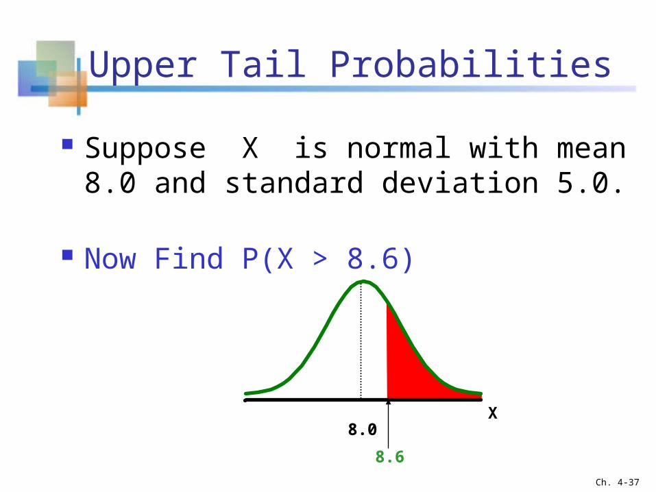
Suppose X is normal with mean 8.0 and standard deviation 5.0.
Now Find P(X > 8.6)
X
8.6
8.0
Ch. 4-37
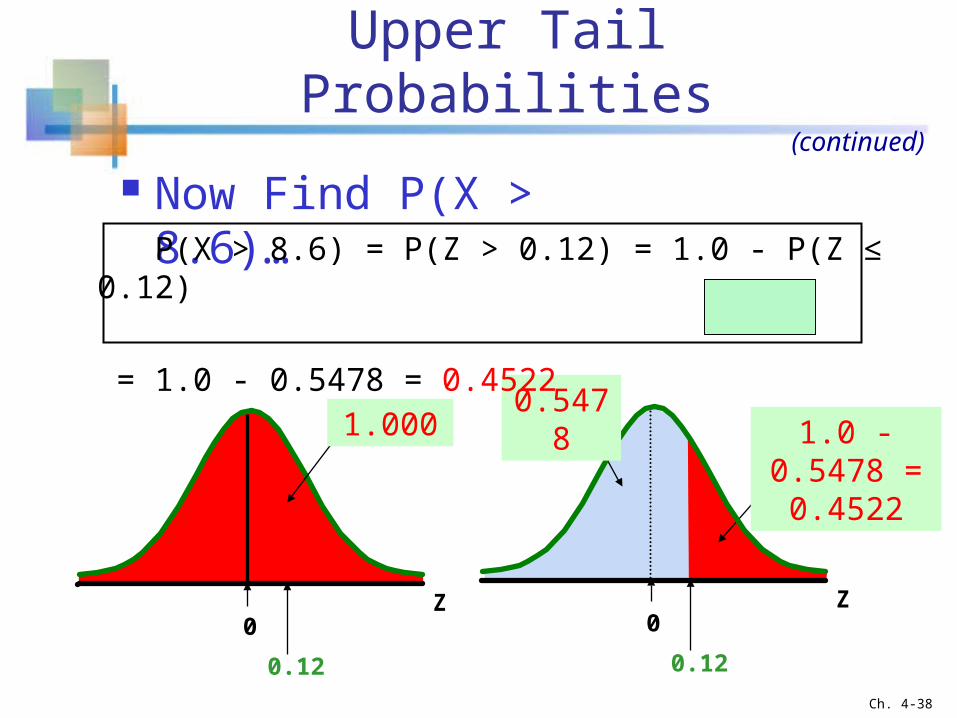
Upper Tail Probabilities
Now Find P(X > 8.6)…(continued)
Z
0.12
0Z
0.12
0.5478
0
1.000 1.0 - 0.5478 = 0.4522
P(X > 8.6) = P(Z > 0.12) = 1.0 - P(Z ≤ 0.12)
= 1.0 - 0.5478 = 0.4522
Ch. 4-38
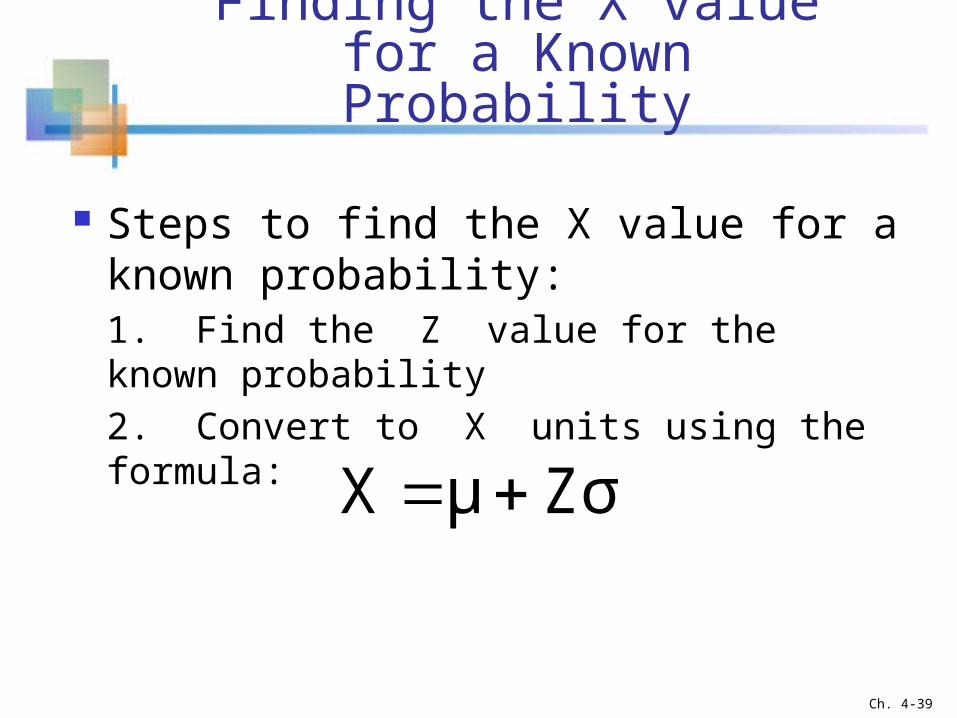
Finding the X value for a Known Probability
Steps to find the X value for a known probability:1. Find the Z value for the known probability
2. Convert to X units using the formula:
ZσμX
Ch. 4-39
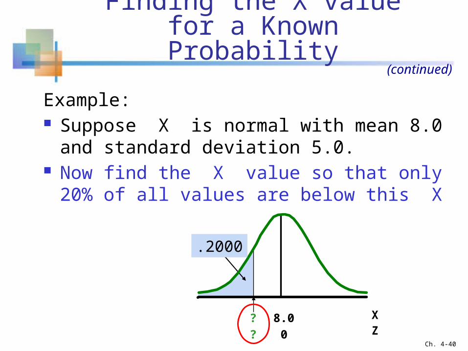
Finding the X value for a Known Probability
Example: Suppose X is normal with mean 8.0 and
standard deviation 5.0. Now find the X value so that only 20% of all
values are below this X
X? 8.0
.2000
Z? 0
(continued)
Ch. 4-40
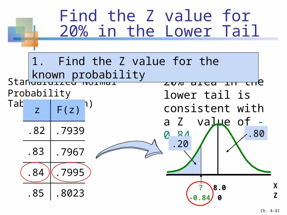
Find the Z value for 20% in the Lower Tail
20% area in the lower tail is consistent with a Z value of -0.84
Standardized Normal Probability Table (Portion)
X? 8.0
.20
Z-0.84 0
1. Find the Z value for the known probability
z F(z)
.82 .7939
.83 .7967
.84 .7995
.85 .8023
.80
Ch. 4-41
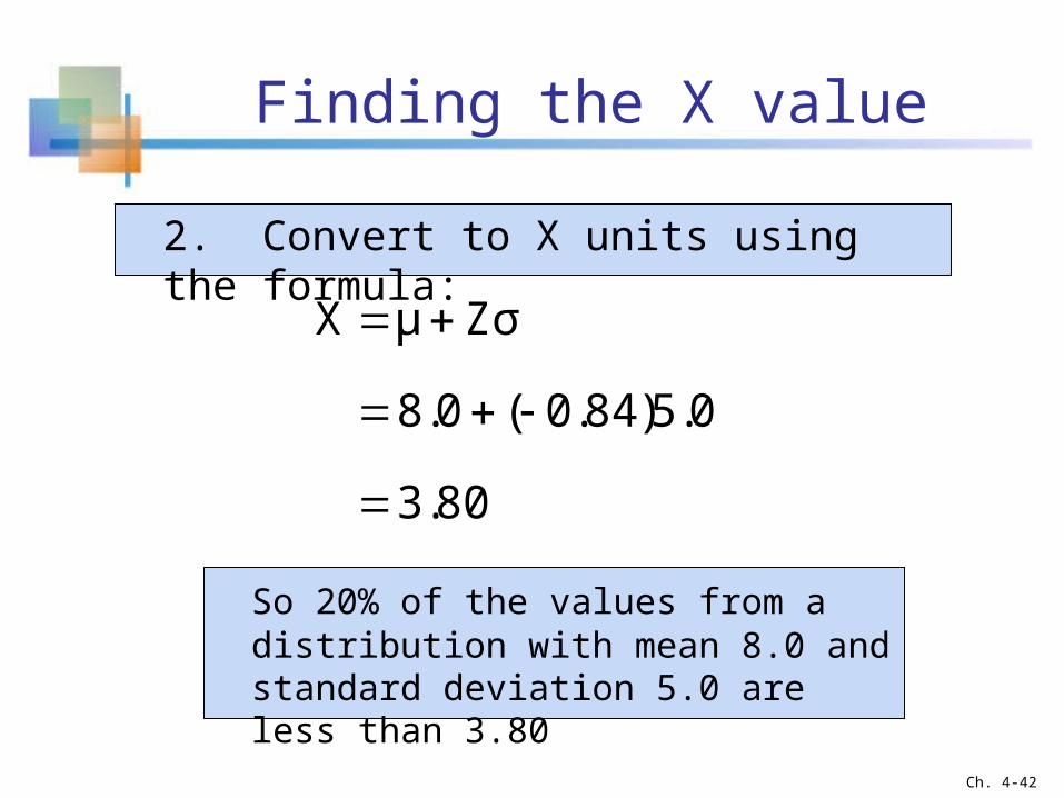
Finding the X value
2. Convert to X units using the formula:
80.3
0.5)84.0(0.8
ZσμX
So 20% of the values from a distribution with mean 8.0 and standard deviation 5.0 are less than 3.80
Ch. 4-42
Assessing Normality
Not all continuous random variables are normally distributed
It is important to evaluate how well the data is approximated by a normal distribution
Ch. 4-43
The Normal Probability Plot
Normal probability plot Arrange data from low to high values Find cumulative normal probabilities for all values Examine a plot of the observed values vs. cumulative
probabilities (with the cumulative normal probability
on the vertical axis and the observed data values on
the horizontal axis) Evaluate the plot for evidence of linearity
Ch. 4-44
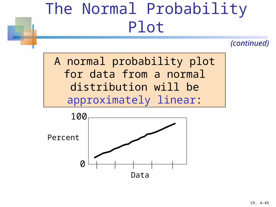
The Normal Probability Plot
A normal probability plot for data from a normal distribution will be
approximately linear:
0
100
Data
Percent
(continued)
Ch. 4-45
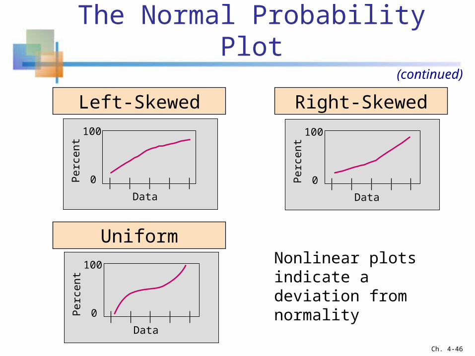
The Normal Probability Plot
Left-Skewed Right-Skewed
Uniform
0
100
Data
Per
cent
(continued)
Nonlinear plots indicate a deviation from normality
0
100
Data
Per
cent
0
100
Data
Per
cent
Ch. 4-46
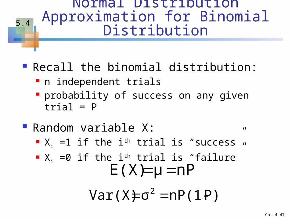
Normal Distribution Approximation for Binomial Distribution
Recall the binomial distribution: n independent trials probability of success on any given trial = P
Random variable X: Xi =1 if the ith trial is “success” Xi =0 if the ith trial is “failure”
nPμE(X)
P)nP(1-σVar(X) 2 Ch. 4-47
5.4
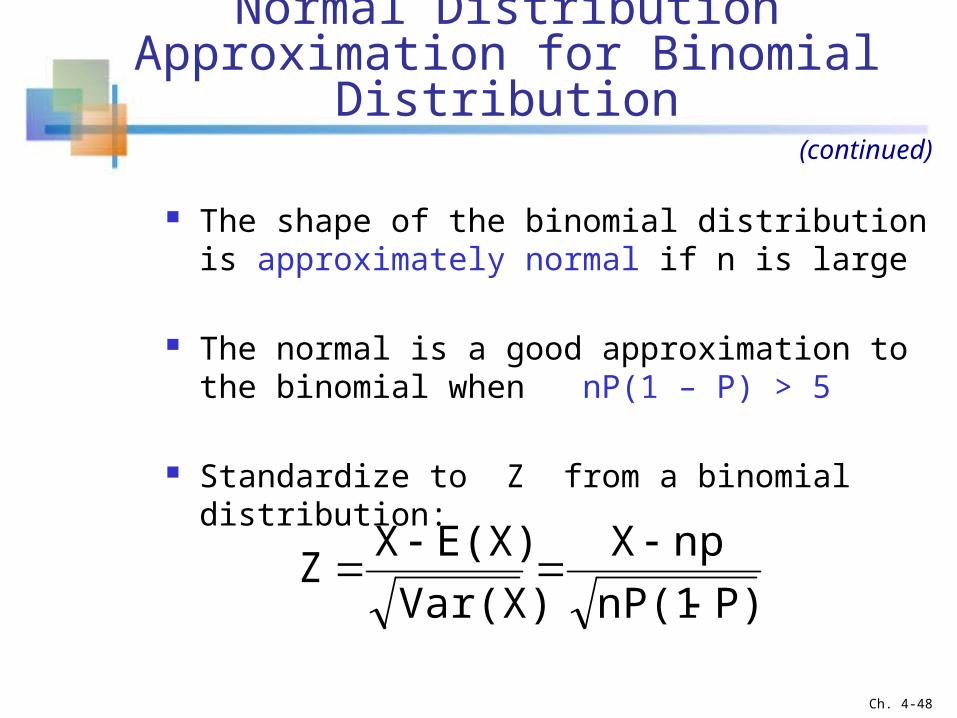
The shape of the binomial distribution is approximately normal if n is large
The normal is a good approximation to the binomial when nP(1 – P) > 5
Standardize to Z from a binomial distribution:
Normal Distribution Approximation for Binomial Distribution
P)nP(1
npX
Var(X)
E(X)XZ
(continued)
Ch. 4-48
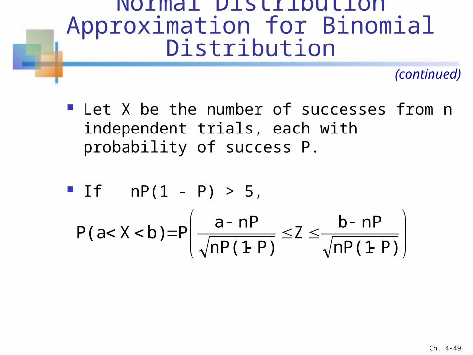
Normal Distribution Approximation for Binomial Distribution
P)nP(1
nPbZ
P)nP(1
nPaPb)XP(a
Let X be the number of successes from n independent trials, each with probability of success P.
If nP(1 - P) > 5,
(continued)
Ch. 4-49
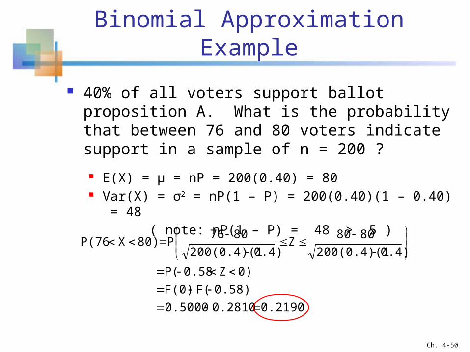
Binomial Approximation Example
0.21900.28100.5000
0.58)F(F(0)
0)Z0.58P(
0.4)200(0.4)(1
8080Z
0.4)200(0.4)(1
8076P80)XP(76
40% of all voters support ballot proposition A. What is the probability that between 76 and 80 voters indicate support in a sample of n = 200 ?
E(X) = µ = nP = 200(0.40) = 80 Var(X) = σ2 = nP(1 – P) = 200(0.40)(1 – 0.40) = 48
( note: nP(1 – P) = 48 > 5 )
Ch. 4-50
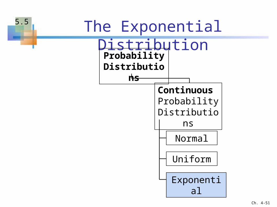
The Exponential Distribution
Continuous Probability
Distributions
Probability Distributions
Normal
Uniform
Exponential
Ch. 4-51
5.5
The Exponential Distribution
Used to model the length of time between two occurrences of an event (the time between arrivals)
Examples: Time between trucks arriving at an unloading dock Time between transactions at an ATM Machine Time between phone calls to the main operator
Ch. 4-52
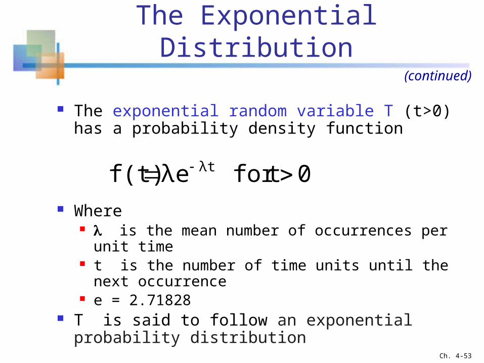
The Exponential Distribution
0 t for ef(t) t λλ
The exponential random variable T (t>0) has a probability density function
Where is the mean number of occurrences per unit time t is the number of time units until the next occurrence e = 2.71828
T is said to follow an exponential probability distribution
(continued)
Ch. 4-53
The Exponential Distribution
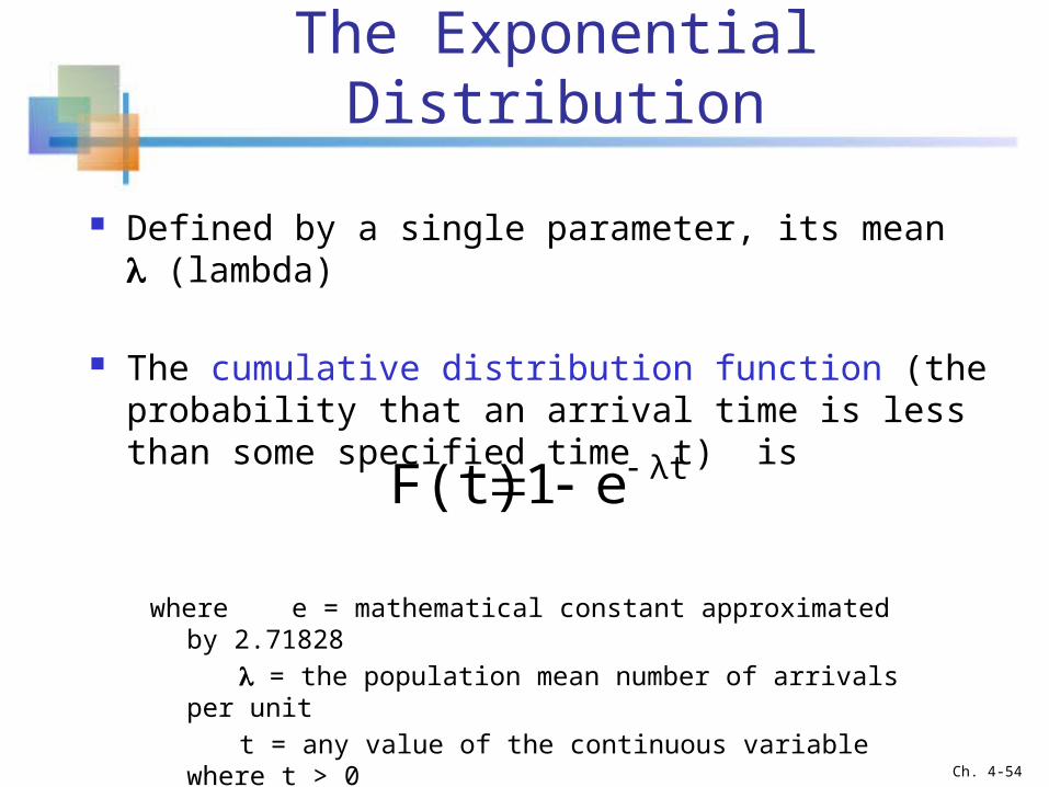
Defined by a single parameter, its mean (lambda)
The cumulative distribution function (the probability that an arrival time is less than some specified time t) is
te1F(t) λ
where e = mathematical constant approximated by 2.71828
= the population mean number of arrivals per unit
t = any value of the continuous variable where t > 0
Ch. 4-54
Exponential Distribution Example
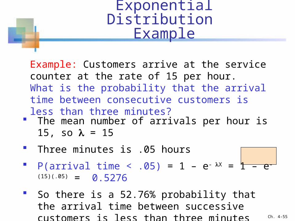
Example: Customers arrive at the service counter at the rate of 15 per hour. What is the probability that the arrival time between consecutive customers is less than three minutes?
The mean number of arrivals per hour is 15, so = 15
Three minutes is .05 hours
P(arrival time < .05) = 1 – e- X = 1 – e-(15)(.05) = 0.5276
So there is a 52.76% probability that the arrival time between successive customers is less than three minutes
Ch. 4-55