Embed Size (px)
Citation preview

Chapter 4
Market Demand and Elasticity
© 2004 Thomson Learning/South-Western

2
Market Demand Curves
The market demand is the total quantity of a good or service demanded by all potential buyers.
The market demand curve is the relationship between the total quantity demanded of a good or service and its price, holding all other factors constant.
3
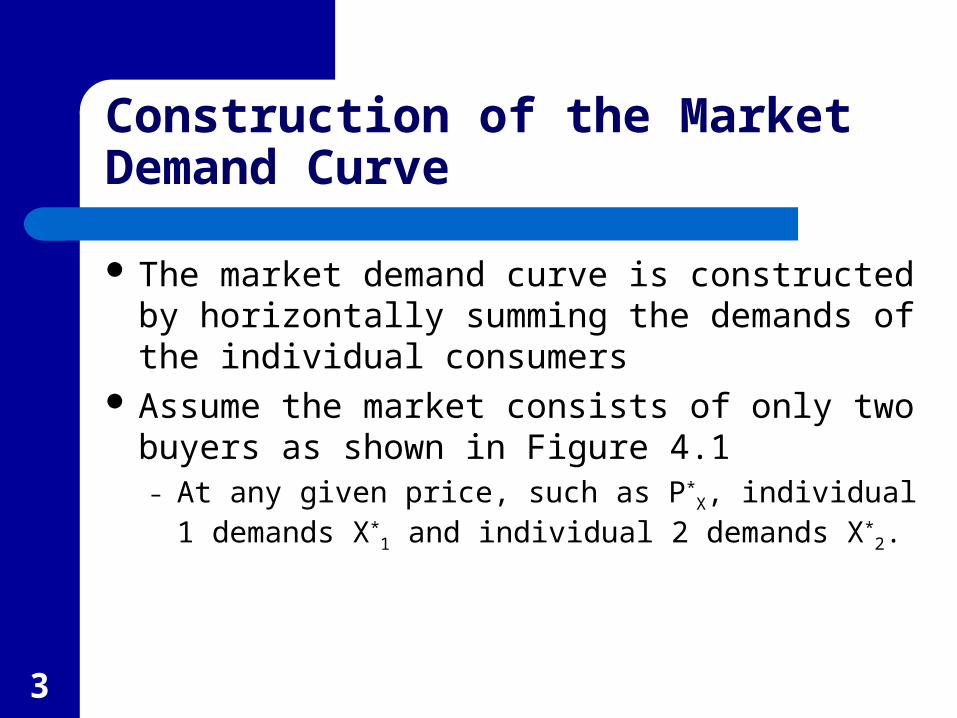
Construction of the Market Demand Curve
The market demand curve is constructed by horizontally summing the demands of the individual consumers
Assume the market consists of only two buyers as shown in Figure 4.1– At any given price, such as P*
X, individual 1 demands X*
1 and individual 2 demands X*2.
4
(a) Individual 1
PX
XP*
X*1
0
(b) Individual 2
X*2
0
(c) Market Demand
X
D
X*0
FIGURE 4.1: Constructing a Market Demand Curve from Individual Demand Curves
PX PX
5
Shifts in the Market Demand Curve
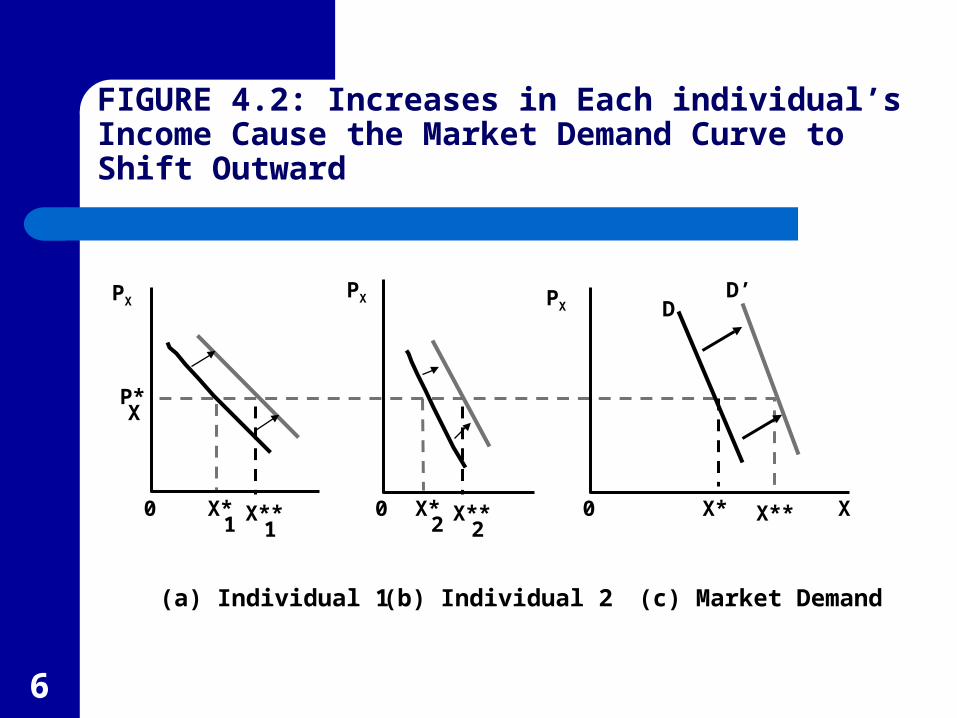
To discover how some event might shift a market demand curve, we must first find out how this event causes individual demand curves to shift and then compare the horizontal sum of these new demand curves with the old demand curve.
6
(a) Individual 1
PX
XP*
X*1
0
(b) Individual 2
X*2
0
(c) Market Demand
X
D
X*0
FIGURE 4.2: Increases in Each individual’s Income Cause the Market Demand Curve to Shift Outward
PX PX
X** X** X**
D’
1 2
7
Shifts in the Market Demand Curve
However, some events result in ambiguous outcomes.– If one consumer’s demand curve shifts out while
another’s shifts in, the net effect depends on the size of the relative shifts.
An increase in income for pizza lovers would increase the market demand for pizza so long as it is a normal good.
8
Shifts in the Market Demand Curve
If goods X and Y are substitutes, an increase in the price of Y will increase the demand for X. Similarly, a decrease in the price of Y will decrease the demand for X.
If goods X and Y are complements, an increase in the price of Y will decrease the demand for X. A decrease in the price of Y will increase the demand for X.
9
APPLICATION 4.1: Consumption and Income Taxes
People’s ability to purchased goods and services is dependent upon their after tax income.
In the 1950’s Milton Friedman argued that people’s consumption decisions are based mostly on their long-term (permanent) income.
10
APPLICATION 4.1: Consumption and Income Taxes
One implication of the permanent-income hypothesis is that temporary tax changes will have little effect on the demand for consumption goods– This prediction is supported by the small impact on
consumption by both the temporary tax surcharge during the Nixon administration and the Ford administration’s temporary income tax rebate
11
A Word on Notation and Terms
When looking at only one market, Q is used for the quantity of the good demanded, and P is used for its price.
When drawing the demand curve, all non-price factors are assumed to not change.
Movements along the curve are changes in quantity demanded, while shifts are changes in demand.
12
Elasticity
Goods are often measured in different units (steak is measured in pounds while oranges are measured in dozens).
It can be difficult to make simple comparisons between goods when trying to determine which is more responsive to changes in price.
13
Elasticity
Elasticity is a measure of the percentage change in one variable brought about by a 1 percent change in some other variable.
Since it is measured in percentages, the units cancel out so that it is a unit-less measure of responsiveness.
14
Price Elasticity of Demand
The price elasticity of demand is the percentage change in the quantity demanded of a good in response to a 1 percent change in its price
Pin change Percentage
Q in change Percentagedemand of elasticity Price , PQe

15
TABLE 4.1: Terminology for the Ranges of eQ,P
Value of eQ,P at a Pointon Demand Curve
Terminology for Curveat This Point
eQ,P < -1 Elastic
eQ,P = -1 Unit elastic
eQ,P > -1 Inelastic
16
Price Elasticity and the Shape of the Demand Curve
We often classify market demand curves by their elasticities– For example, the market demand curve for
medical services is inelastic (nearly vertical) since there is little quantity response to changes in price.
– Alternatively, the market demand curve for a single type of candy bar is very responsive to price change (nearly flat) and is very elastic.
17
Price Elasticity and the Substitution Effect
Goods which have many close substitutes are subject to large substitution effects from a price change so their market demand curve is likely to be relatively elastic.
Goods with few close substitutes, on the other hand, will likely be relatively inelastic.
18
Price Elasticity and Time
Some items can be quickly substituted for, such as a brand of breakfast cereal, others, such as heating fuel, may take several years.
Thus, in some situations, it is important to make the distinction between the short-term and long-term elasticities of demand.
19
APPLICATION 4.2: Brand Loyalty
Substitution due to price changes will likely take a longer time if individual’s develop spending habits.
Such brand loyalties are rational since they reduce decision making costs.
Over the long term, however, price differences may cause buyers to try other brands.
20
Price Elasticity and Total Expenditures
Total expenditures on a good are found by multiplying the good’s price (P) times the quantity purchased (Q).
When demand is elastic, price increases will cause total expenditures to fall.– The given percentage increase in price is more than
counterbalanced by the decrease in quantity demanded.
21
Price Elasticity and Total Expenditures
Of course, when demand is elastic and prices fall, total expenditures increase.
With unit elasticity, total expenditures remain the same with a price change.– The movement in one direction by the price is fully
offset by the movement in the other direction with the quantity demanded.
22
TABLE 4.2: Relationship between Price Changes and Changes in Total Expenditure
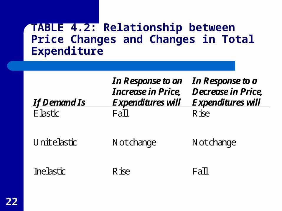
If Demand Is
In Response to an Increase in Price, Expenditures will
In Response to a Decrease in Price, Expenditures will
Elastic Fall Rise
Unit elastic Not change Not change
Inelastic Rise Fall
23
APPLICATION 4.3: Volatile Farm Prices
The demand for many basic agricultural products (wheat, corn, etc.) is relatively inelastic.
Even modest changes in supply, brought about by weather patterns, can have large effects on crop prices.
24
Demand Curves and Price Elasticity
The relationship between a particular demand curve and the price elasticity it exhibits can be complicated.
For some curves, the elasticity remains constant everywhere, but for others it is different at every point.
A more accurate way to describe it would be to say the elasticity is for current prices.
25
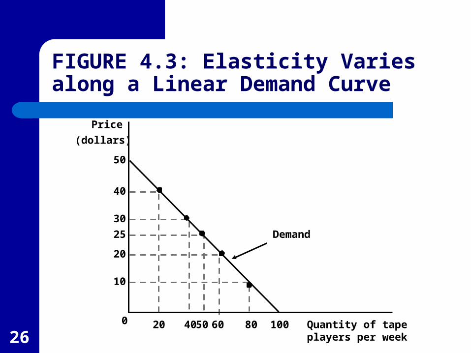
Linear Demand Curves and Price Elasticity
The price elasticity of demand is always changing along a straight line demand curve.– Demand is elastic at prices above the midpoint
price.– Demand is unit elastic at the midpoint price.– Demand is inelastic at prices below the midpoint
price.
26
Price
(dollars)
10
50
40
30
25
20
Quantity of tape players per week
Demand
20 405060 80 1000
FIGURE 4.3: Elasticity Varies along a Linear Demand Curve
27
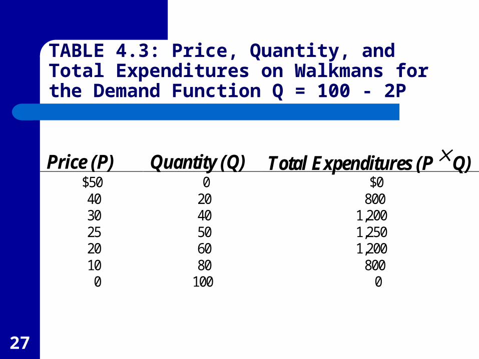
TABLE 4.3: Price, Quantity, and Total Expenditures on Walkmans for the Demand Function Q = 100 - 2P
Price (P) Quantity (Q) Total Expenditures (P Q)$50 0 $0 40 20 800 30 40 1,200 25 50 1,250 20 60 1,200 10 80 800 0 100 0
28
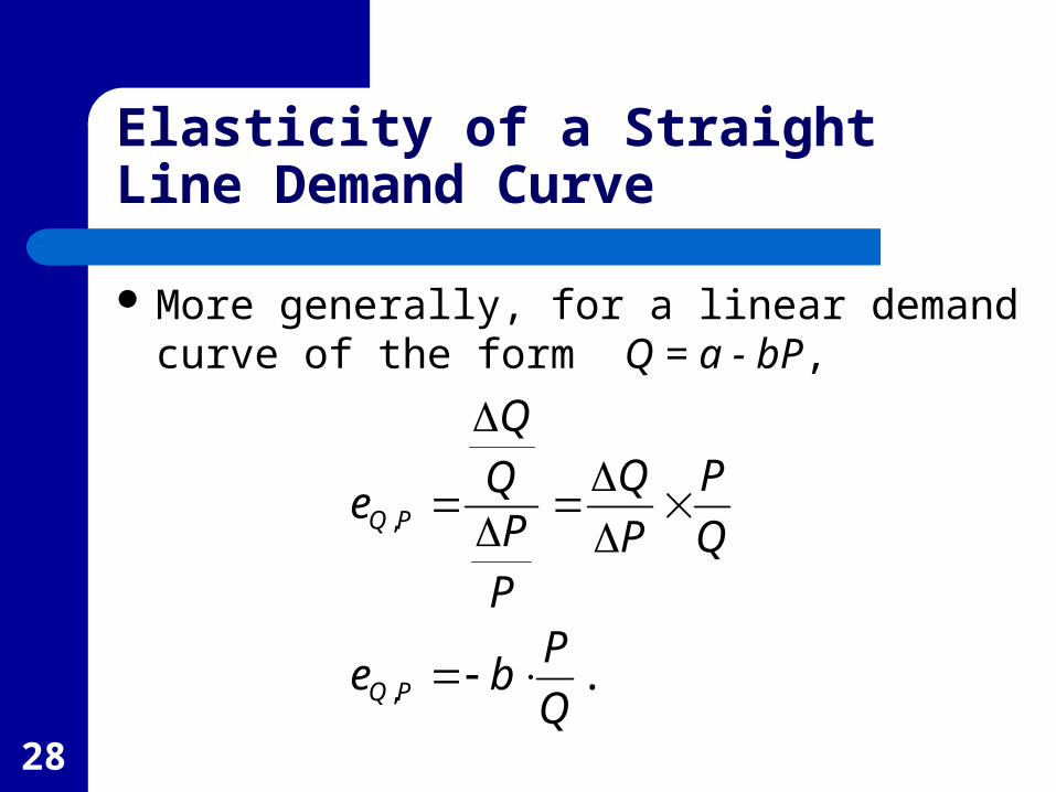
Elasticity of a Straight Line Demand Curve
.,
,
Q
Pbe
Q
P
P
Q
P
PQ
Q
e
PQ
PQ
More generally, for a linear demand curve of the form Q = a - bP,
29
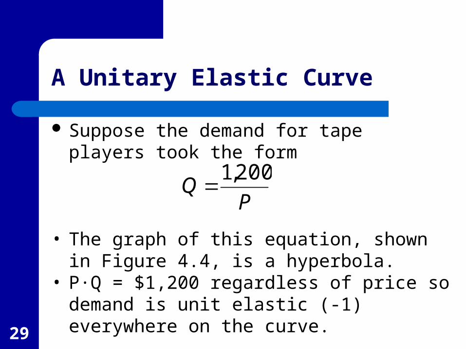
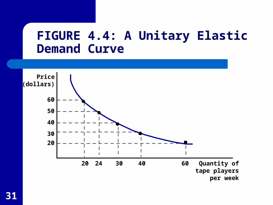
A Unitary Elastic Curve
Suppose the demand for tape players took the form
PQ
200,1
• The graph of this equation, shown in Figure 4.4, is a hyperbola.
• P·Q = $1,200 regardless of price so demand is unit elastic (-1) everywhere on the curve.
30
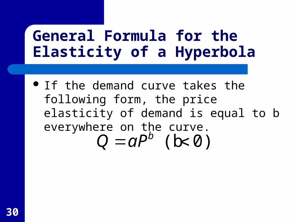
General Formula for the Elasticity of a Hyperbola
If the demand curve takes the following form, the price elasticity of demand is equal to b everywhere on the curve.
0) (b baPQ
31
Price(dollars)
20
60
50
40
30
Quantity oftape players
per week
20 24 30 40 60
FIGURE 4.4: A Unitary Elastic Demand Curve
32
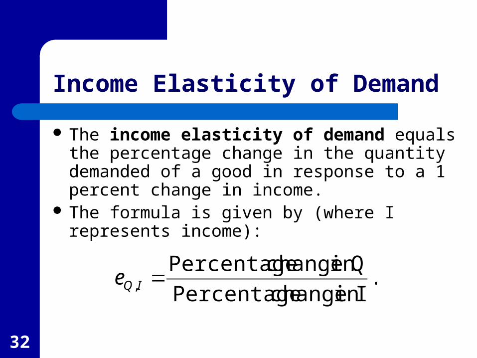
Income Elasticity of Demand
The income elasticity of demand equals the percentage change in the quantity demanded of a good in response to a 1 percent change in income.
The formula is given by (where I represents income):
.Iin change Percentage
Qin change Percentage, IQe
33
Income Elasticity of Demand
For normal goods, eQ,I is positive because increases in income lead to increases in purchases of the good.
For inferior goods eQ,I is negative.
If eQ,I > 1, the purchase of the good increases more rapidly than income so the good might be called a luxury good.

34
APPLICATION 4.4: An Experiment in Health Insurance
Most developed countries have some form of national health insurance.– In the U.S. Medicare covers the elderly and
Medicaid is available for many of the poor.
Recently a number of comprehensive government health plans have been proposed.

35
The Moral Hazard Problem
A “moral hazard” problem occurs because insurance misleadingly lowers the out-of-pocket expenses to patients, greatly increasing their demand for medical services.
An important question, in considering implementing national health insurance is how large an increase is likely to develop?
36
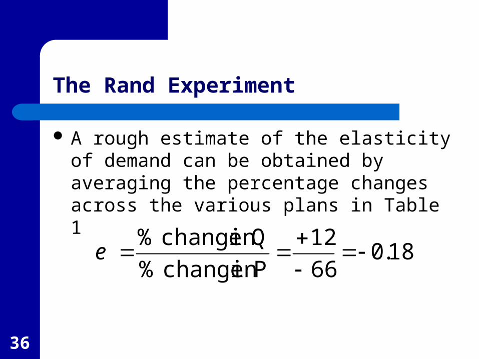
The Rand Experiment
A rough estimate of the elasticity of demand can be obtained by averaging the percentage changes across the various plans in Table 1
18.066
12
Pin change %
Qin change %
e

37
Low Elasticities for Hospital and Doctors’ Visits
Using the estimate of -0.22 found in Table 4.4, and based on other studies suggests only a small increase in hospital and doctor visits would result from the lower prices provided by insurance.
Alternatively, researchers have found greater elasticities (around -0.5) for dental care and outpatient mental health care.
38
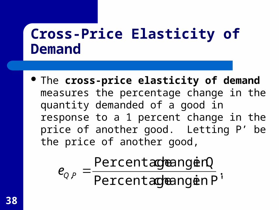
Cross-Price Elasticity of Demand
The cross-price elasticity of demand measures the percentage change in the quantity demanded of a good in response to a 1 percent change in the price of another good. Letting P’ be the price of another good,
. P'in change Percentage
Q in change Percentage, PQe
39
Cross-Price Elasticity of Demand
If the goods are substitutes, an increase in the price of one will cause buyers to purchase more of the substitute, so the elasticity will be positive.
If the goods are complements, an increase in the price of one will cause buyers to buy less of that good and also less of the good they use with it, so the elasticity will be negative
40
Empirical Studies of Demand: Estimating Demand Curves
Estimating a demand curve for a product is one of the more difficult but important problems in econometrics.
Empirical studies are useful because they a provide a more precise estimate of the amount of change in quantity demanded that results due to a price change.
41
Problems Estimating Demand Curves
The first problem is how to derive an estimate holding all other factors (the ceteris paribus assumption) constant.
This problem is often solved, as discussed in the Appendix to Chapter 1, by the use of multiple regression analysis.
42
Problems Estimating Demand Curves
The second problem deals with what is observed in the data. The data points represent quantity and price outcomes that are simultaneously determined by both the demand and the supply curves.
The econometric problem is to “identify” from these equilibrium points the demand curve that generated them.
43
Some Elasticity Estimates
Table 4.4 gathers a number of estimated income and price elasticities of demand.
Some things to note– All of the estimated price elasticities are less than
zero as predicted by a negatively sloped demand curve.
– Most of the price elasticity estimates are inelastic.
44
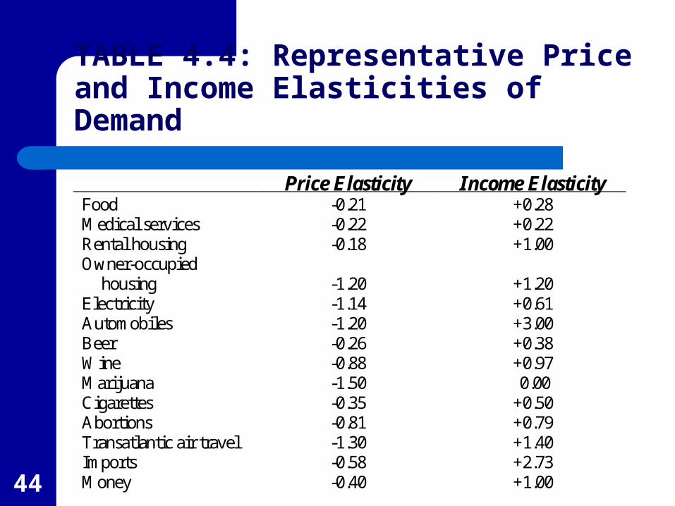
TABLE 4.4: Representative Price and Income Elasticities of Demand
Price Elasticity Income Elasticity Food -0.21 +0.28 Medical services -0.22 +0.22 Rental housing -0.18 +1.00 Owner-occupied
housing
-1.20
+1.20 Electricity -1.14 +0.61 Automobiles -1.20 +3.00 Beer -0.26 +0.38 Wine -0.88 +0.97 Marijuana -1.50 0.00 Cigarettes -0.35 +0.50 Abortions -0.81 +0.79 Transatlantic air travel -1.30 +1.40 Imports -0.58 +2.73 Money -0.40 +1.00
45
Some Elasticity Estimates
The income elasticities of automobiles and transatlantic travel exceed 1 (luxuries).
The high income elasticities are balanced by goods such as food and medical care which are less than 1 (necessities).
There is no evidence of Giffen’s paradox in the table.
46
Some Cross-price Elasticity Estimates
Table 4.5 shows a few cross-price elasticity estimates
All of the goods appear to be substitutes and have positive cross-price elasticities.
47
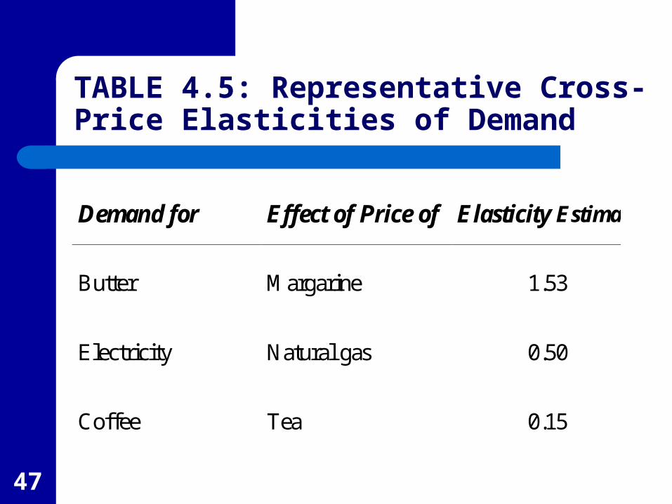
TABLE 4.5: Representative Cross-Price Elasticities of Demand
Demand for Effect of Price of Elasticity Estimate
Butter Margarine 1.53
Electricity Natural gas 0.50
Coffee Tea 0.15
48
Application 4.5: Alcohol Taxes as Drunk Driving Policy
Each year more than 40,000 Americans die in automobile accidents.
It is generally believed that alcohol consumption is a major contributing factor in at least half of those accidents.
Most empirical studies of alcohol consumption show that it is sensitive to price.

49
Application 4.5: Alcohol Taxes as Drunk Driving Policy
The figures in Table 4.4 suggest that these elasticities range from approximately –0.3 for beer to perhaps as large as –0.9 for wine.
Most teenage alcohol consumption is beer. The lower price elasticity of demand for beer
poses a problem for those who would use alcohol taxes as a deterrent to drunk driving.