72

Chapter 4

Asymptotic Solutions for the General Meridian

The cylindrical shell is the one case for which the equations, whether in the form of two coupled equations of second order (2.11.3-4), a single complex equation of the second order (2.11.11), or a matrix system (2.11.22), have only constant coefficients. The exact, general complementary solution can be obtained as a sum of exponentials. For any other meridian, the coefficients vary with the arc length. For certain special cases, solutions can be obtained in terms of special functions. However, in the single complex equation (2.11.11) the highest derivative term is seen to be multiplied by the thickness. In the limit of the thickness approaching zero, while the geometry of the reference surface remains fixed, the high derivative term disappears and the order of the equation is reduced, in this case from second to zero order. This is the characteristic of a singular perturbation problem. So, while it is in general a difficult task to find exact solutions for equations with varying coefficients, it is often possible in singular perturbation problems to obtain approximate solutions of a wide range of useful validity. Various aspects of the approach can be found in many fields of science and engineering. Interesting and useful condensation of much material is given by Olver (1983) and Carrier (1983). Applications in fluid mechanics are in the text by Van Dyke (1964). In this section, only the aspects which are directly applicable to the shell problem will be discussed. §4.1 Scaling of Equations For the matrix equation, the first task is to organize the matrix into a better form by an appropriate scaling of the elements in the array (2.11.23). It is convenient to make the physical quantities dimensionless by multiplying each by a suitable constant. A convenient choice for the constant is to make each have the magnitude of the rotation. From the preceding results for the cylindrical shell and other considerations, i.e., we have looked ahead and know how the solutions work out, the choice for the dimensionless version of (2.11.23) is

y =

r M s λr E t c e

r HE t c e

χ

h λr e (4.1.1)

in which the subscript 'e' denotes that the quantity is evaluated at a specific point of the meridian, (i.e., the 'edge'), and the large parameter of the problem is the square root of the

73

radius-to-thickness ratio:

λ =

r2c e

12

(4.1.2) In addition the dimensionless arc length x is used:

x = s

r2 e (4.1.3) By suitable multiplication of the rows and columns in the system (2.11.22) the matrix equation becomes

– d yλ d x

+ a •y = b (4.1.4)

in which the coefficient matrix and the load vector have the expansions as powers of the large parameter:

a = a 0 +λ– 1a 1 + λ

– 2a 2

b = b 0 +λ– 1b 1 + λ

– 2b 2 (4.1.5-6)

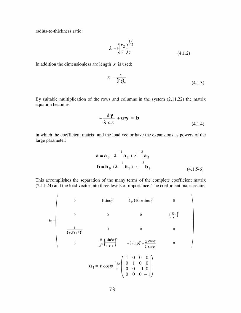
This accomplishes the separation of the many terms of the complete coefficient matrix (2.11.24) and the load vector into three levels of importance. The coefficient matrices are

a0 =

0 sinϕ * 2 ρ E t c sinϕ * 0

0 0 0 E t r

*

1 r E t c 2 *

0 0 0

0µ

λ2

sin2ϕ

r Ε t

∗

– sinϕ * – χ cosϕ2 sinϕe

0

a 1 = ν cosϕr2er

1 0 0 00 1 0 00 0 – 1 00 0 0 – 1

74

a 2 =1 – ν

2cos2ϕ

sin2ϕ e

0 0 E t c2

r

*

0

0 0 0 0

0 0 0 0

0 1

r E t* 0 0

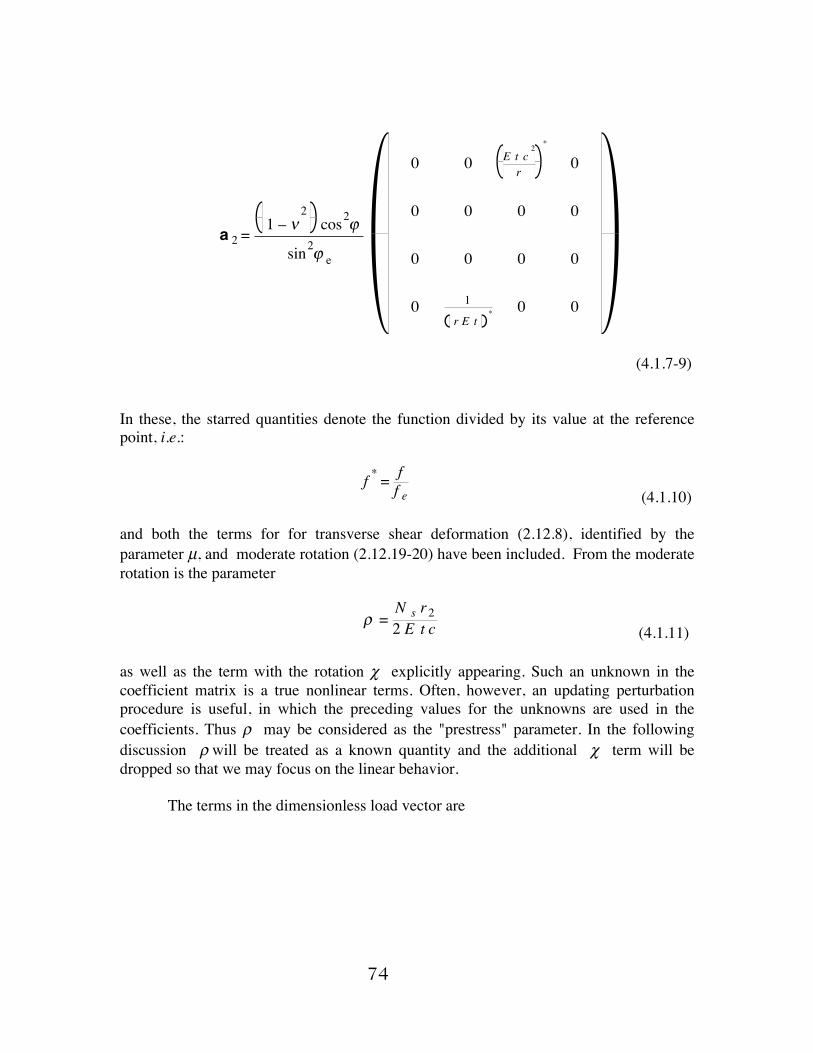
(4.1.7-9) In these, the starred quantities denote the function divided by its value at the reference point, i.e.:

f * = f

f e (4.1.10) and both the terms for for transverse shear deformation (2.12.8), identified by the parameter µ, and moderate rotation (2.12.19-20) have been included. From the moderate rotation is the parameter

ρ =

N s r22 E t c (4.1.11)

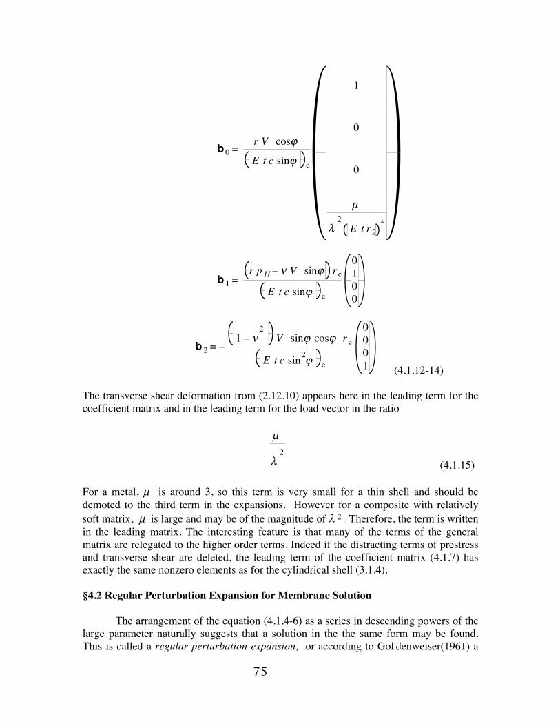
as well as the term with the rotation χ explicitly appearing. Such an unknown in the coefficient matrix is a true nonlinear terms. Often, however, an updating perturbation procedure is useful, in which the preceding values for the unknowns are used in the coefficients. Thus ρ may be considered as the "prestress" parameter. In the following discussion ρ will be treated as a known quantity and the additional χ term will be dropped so that we may focus on the linear behavior. The terms in the dimensionless load vector are

75

b 0 =r V cosϕ

E t c sinϕ e

1

0

0

µ

λ2E t r2

*

b 1 =r p H – ν V sinϕ r e

E t c sinϕ e

0100

b 2 = –1 – ν

2V sinϕ cosϕ r e

E t c sin2ϕ e

0001 (4.1.12-14)

The transverse shear deformation from (2.12.10) appears here in the leading term for the coefficient matrix and in the leading term for the load vector in the ratio

µ

λ2

(4.1.15) For a metal, µ is around 3, so this term is very small for a thin shell and should be demoted to the third term in the expansions. However for a composite with relatively soft matrix, µ is large and may be of the magnitude of λ 2 . Therefore, the term is written in the leading matrix. The interesting feature is that many of the terms of the general matrix are relegated to the higher order terms. Indeed if the distracting terms of prestress and transverse shear are deleted, the leading term of the coefficient matrix (4.1.7) has exactly the same nonzero elements as for the cylindrical shell (3.1.4). §4.2 Regular Perturbation Expansion for Membrane Solution The arrangement of the equation (4.1.4-6) as a series in descending powers of the large parameter naturally suggests that a solution in the the same form may be found. This is called a regular perturbation expansion, or according to Gol'denweiser(1961) a

76

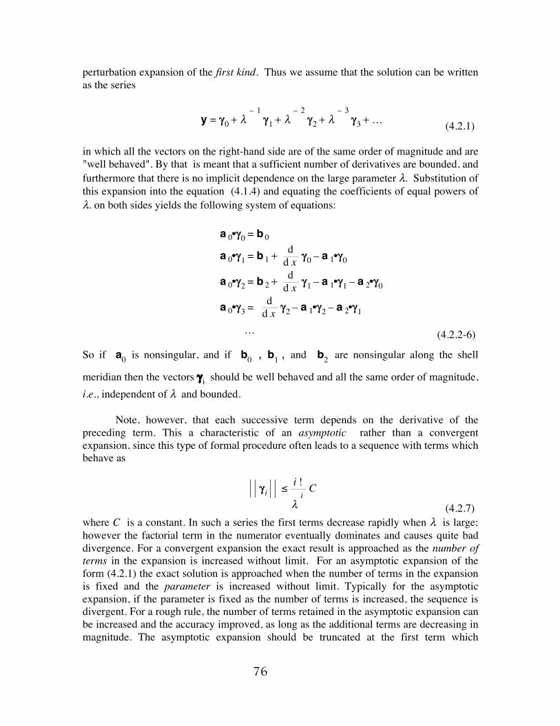
perturbation expansion of the first kind. Thus we assume that the solution can be written as the series

y = γ0 + λ– 1

γ1 + λ– 2

γ2 + λ– 3

γ3 + .. . (4.2.1) in which all the vectors on the right-hand side are of the same order of magnitude and are "well behaved". By that is meant that a sufficient number of derivatives are bounded, and furthermore that there is no implicit dependence on the large parameter λ. Substitution of this expansion into the equation (4.1.4) and equating the coefficients of equal powers of λ. on both sides yields the following system of equations:

a 0•γ0 = b 0a 0•γ1 = b 1 +

dd x γ0 – a 1•γ0

a 0•γ2 = b 2 +dd x γ1 – a 1•γ1 – a 2•γ0

a 0•γ3 =dd x γ2 – a 1•γ2 – a 2•γ1

. . . (4.2.2-6)

So if a 0 is nonsingular, and if b

0 , b 1 , and b

2 are nonsingular along the shell

meridian then the vectors γ i should be well behaved and all the same order of magnitude,

i.e., independent of λ and bounded. Note, however, that each successive term depends on the derivative of the preceding term. This a characteristic of an asymptotic rather than a convergent expansion, since this type of formal procedure often leads to a sequence with terms which behave as

γ i ≤ i !

λiC

(4.2.7) where C is a constant. In such a series the first terms decrease rapidly when λ is large; however the factorial term in the numerator eventually dominates and causes quite bad divergence. For a convergent expansion the exact result is approached as the number of terms in the expansion is increased without limit. For an asymptotic expansion of the form (4.2.1) the exact solution is approached when the number of terms in the expansion is fixed and the parameter is increased without limit. Typically for the asymptotic expansion, if the parameter is fixed as the number of terms is increased, the sequence is divergent. For a rough rule, the number of terms retained in the asymptotic expansion can be increased and the accuracy improved, as long as the additional terms are decreasing in magnitude. The asymptotic expansion should be truncated at the first term which

77

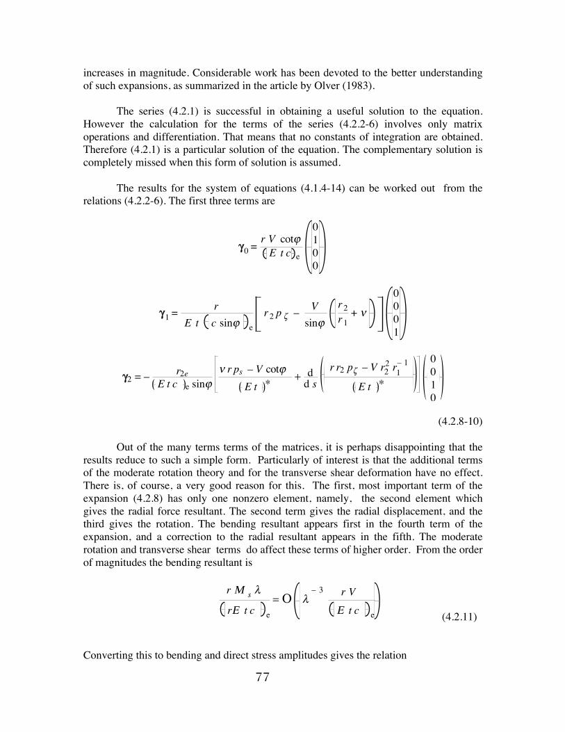
increases in magnitude. Considerable work has been devoted to the better understanding of such expansions, as summarized in the article by Olver (1983). The series (4.2.1) is successful in obtaining a useful solution to the equation. However the calculation for the terms of the series (4.2.2-6) involves only matrix operations and differentiation. That means that no constants of integration are obtained. Therefore (4.2.1) is a particular solution of the equation. The complementary solution is completely missed when this form of solution is assumed. The results for the system of equations (4.1.4-14) can be worked out from the relations (4.2.2-6). The first three terms are

γ0 =r V cotϕE t c e

0100

γ1 =r

E t c sinϕ er2 p ζ –

Vsinϕ

r2r1+ ν

0001

γ2 = – r2e E t c e sinϕ

ν r ps – V cotϕ E t * + d

d s r r2 pζ – V r2

2 r1– 1

E t * 0010

(4.2.8-10) Out of the many terms terms of the matrices, it is perhaps disappointing that the results reduce to such a simple form. Particularly of interest is that the additional terms of the moderate rotation theory and for the transverse shear deformation have no effect. There is, of course, a very good reason for this. The first, most important term of the expansion (4.2.8) has only one nonzero element, namely, the second element which gives the radial force resultant. The second term gives the radial displacement, and the third gives the rotation. The bending resultant appears first in the fourth term of the expansion, and a correction to the radial resultant appears in the fifth. The moderate rotation and transverse shear terms do affect these terms of higher order. From the order of magnitudes the bending resultant is

r Μ s λ

rΕ t c e

= Ο λ– 3 r V

Ε t c e (4.2.11) Converting this to bending and direct stress amplitudes gives the relation

78

σ B = Ο λ– 2

σ D (4.2.12) Thus the bending stress is small in comparison with the direct stress in the shell. The shell is carrying the surface and axial load by stretching and compression of the wall rather than by bending, just as the Roman arch in Fig. 1.4. Because of the lack of significant bending this solution is referred to as the membrane solution. Often the direct stress is called the "membrane" stress; however, as we have seen in the examples of the cylindrical shell, significant direct stress is also associated with the complementary solution. The term "membrane " normally brings the image of a thin wall which can support negligible compressive stress. In fact the masonry Roman arch and the domes in Fig. 1.5 are carrying substantial compressive loads. Thus "membrane behavior" can occur for either tensile or compressive stress, and only indicates a relatively low level of bending stress. This membrane solution can be obtained more easily by just assuming that the transverse shear resultant is small in comparison with the tangential resultants. Indeed when the leading term result (4.2.8) is written back in the original variables, it is just Η = V cotϕ (4.2.13) Thus the tangential resultant, according to this one term level of approximation, is

Ν s = H cosϕ +V sinϕ = V

sinϕ (4.2.14) and the transverse shear resultant is

Q = H sinϕ –V cosϕ = 0 (4.2.15) It is important to realize that this result is the leading term of the expansion. The fifth term of (4.2.1) gives a correction to H in (4.2.14), which will provide a correction to (4.2.15). So a five term solution yields the result that Q is not identically zero but is small:

N s =Vsinϕ

1 + O λ– 4

Q = O λ– 4 Vsinϕ (4.2.16-17)

If Q is initially assumed to be zero, the result (4.2.13) follows directly from (2.4.1) and (4.2.14) from (2.4.2). The equation for normal equilibrium (2.4.13) gives the

79

circumferential resultant:

N θ = r2 p ζ –

r2r1N s = r2 p ζ –

r2r1

Vsinϕ (4.2.18)

and the radial displacement can be calculated from the inverse of (2.8.15-16):

hr = ε θ =

1E t = 1

E t r2 p ζ –r2r1

Vsinϕ

– ν Vsinϕ (4.2.19)

which is, of course, exactly the result (4.2.9). The rotation can be computed from (2.7.3) which agrees with (4.2.10).

80

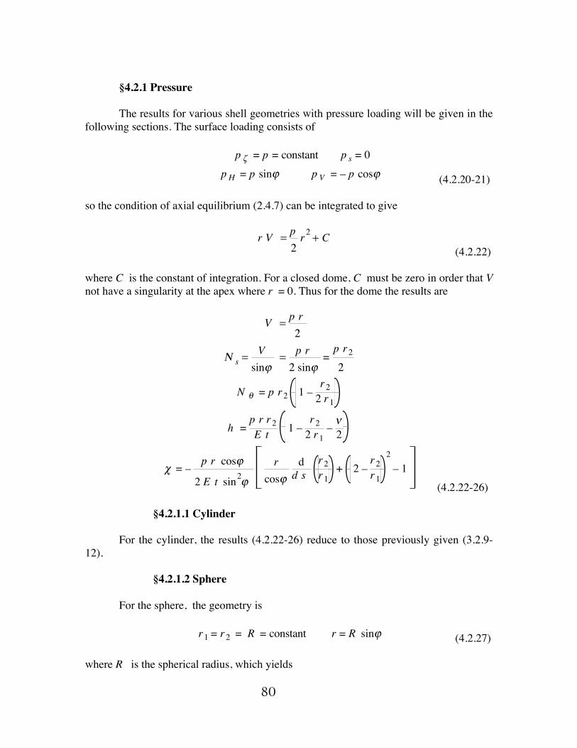
§4.2.1 Pressure The results for various shell geometries with pressure loading will be given in the following sections. The surface loading consists of

p ζ = p = constant p s = 0p H = p sinϕ p V = – p cosϕ (4.2.20-21)

so the condition of axial equilibrium (2.4.7) can be integrated to give

r V = p

2r2 + C

(4.2.22) where C is the constant of integration. For a closed dome, C must be zero in order that V not have a singularity at the apex where r = 0. Thus for the dome the results are

V = p r2

Ν s =Vsinϕ

= p r2 sinϕ

=p r22

N θ = p r2 1 –r22 r1

h =p r r2E t 1 –

r22 r1

– ν2

χ = – p r cosϕ

2 E t sin2ϕ

rcosϕ

dd s

r2r1

+ 2 –r2r1

2

– 1 (4.2.22-26)

§4.2.1.1 Cylinder For the cylinder, the results (4.2.22-26) reduce to those previously given (3.2.9-12). §4.2.1.2 Sphere For the sphere, the geometry is

r1 = r2 = R = constant r = R sinϕ (4.2.27) where R is the spherical radius, which yields

81

N s = N θ =p R2

h = p R2 sinϕ2 E t ( 1– ν )

χ = 0 (4.2.28-30) §4.2.1.3 Cone For the cone, the geometry is

ϕ = constant r1 = ∞ (4.2.31) which gives

N s =p r

2 sinϕ

N θ =p rsinϕ

h = p r2

2 E t sinϕ( 2 – ν )

χ = – 3 p r cosϕ

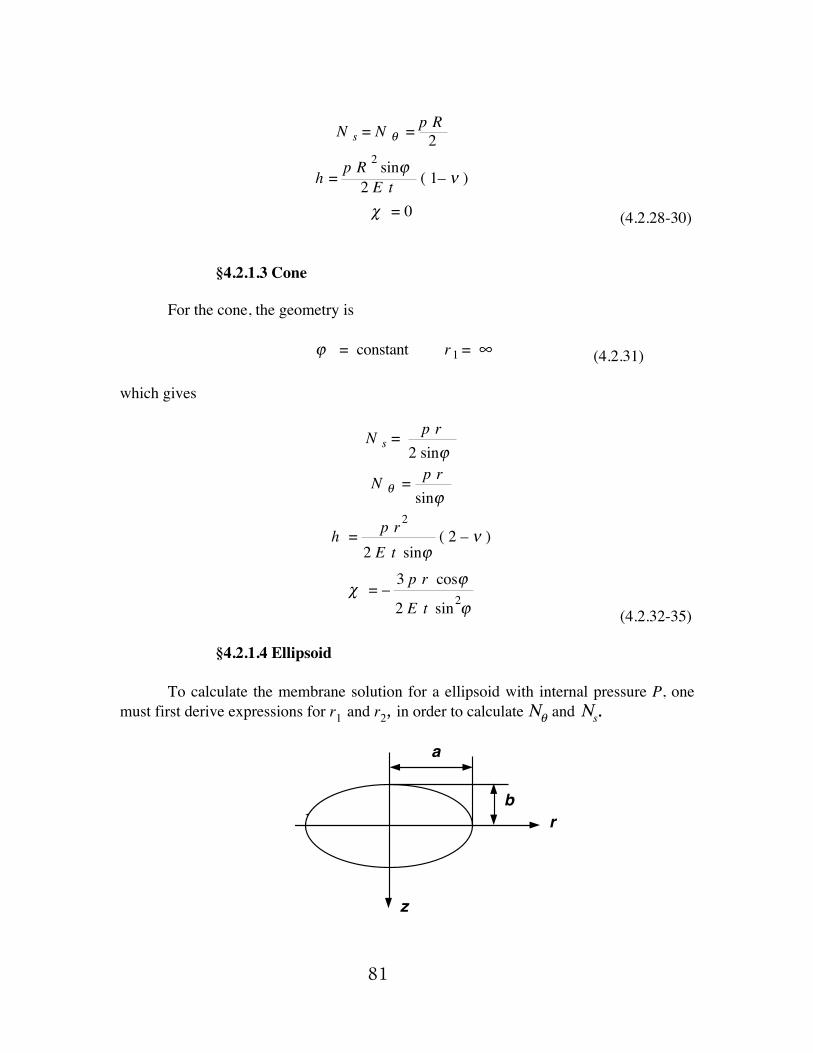
2 E t sin2ϕ (4.2.32-35) §4.2.1.4 Ellipsoid To calculate the membrane solution for a ellipsoid with internal pressure P, one must first derive expressions for r1 and r2, in order to calculate Nθ and Ns.

b

a b

a

z

r

82

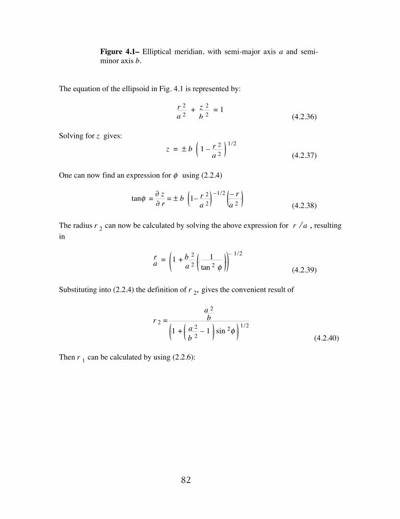
Figure 4.1– Elliptical meridian, with semi-major axis a and semi-minor axis b.

The equation of the ellipsoid in Fig. 4.1 is represented by:

r 2

a 2 + z 2

b 2 = 1

(4.2.36) Solving for z gives:

z = ± b 1 – r 2

a 2

1/2

(4.2.37) One can now find an expression for φ using (2.2.4)

tanφ = ∂ z

∂ r = ± b 1– r 2

a 2

–1/2 – r

a 2

(4.2.38) The radius r 2 can now be calculated by solving the above expression for r /a , resulting in

ra = 1 + b

2

a 2 1

tan 2 φ

– 1/2

(4.2.39) Substituting into (2.2.4) the definition of r 2, gives the convenient result of

r 2 = a 2b

1 + a 2

b 2 – 1 sin 2φ

1/2

(4.2.40) Then r 1 can be calculated by using (2.2.6):

83

r 1 = ∂ s

∂ φ = ∂ r

∂ φ 1

cos φ

=

∂

∂φ r 2 sin φ 1

cos φ =

∂r 2

∂φ tan φ + r 2

(4.2.41)

r 1 = a 2b

1 + a 2

b 2 – 1 sin2 φ

3/2

(4.2.42)

r 2r 1

= 1 + k sin2φ (4.2.43) where

k = a 2

b 2 – 1

84

Now the membrane solution will be:

N s = Pr 2

2 = Pa 2

2b 1 + k sin2 φ 1/2 (4.2.44)

Nθ = Pr 2

2 2 – r 2r 1

= P r 22 1 – k sin2 φ (4.2.45)

So, for k > 1, i.e., a 2 > 2 b 2, Νθ is negative in the region near φ = π / 2. The deformation is given by

hr = P r 2

E t 1 – r 2

2r 1 – ν2

85

= P r 2

2 E t 1 – ν – k sin2φ = P R

2 E t

1 – ν – k sin2 φ

1 + k sin2 φ 1/2 (4.2.46)

where the radius of curvature at the apex is:

R = a2b

The rotation is:

χ = –

P r cosφ2E t sin2 φ

rr 1 cos φ

∂∂φ

r 2r 1

+ 2 – r 2r 1

2 – 1

= P R k

2 E t

cosφ sinφ

1 + k sin2φ 1/2 4 + k sin2φ

(4.2.47) §4.2.1.5 Paraboloid For a parabolic shell, the equation representing the geometry is

z = r 22 R (4.2.48)

The radii of curvature r 1 and r 2 can be calculated by first using equation (2.2.4)

86

∂ z∂ r = r

R = tan φ

(4.2.49) Using (2.2.7) one gets the following expression for r 2

r 2 = Rcos φ

(4.2.50)

To calculate r 1 one must use (2.2.6), resulting in

r 1 = 1

z ′′cos3 φ = R

cos3 φ (4.2.51)

Another interesting way to derive these results can be accomplished by taken certain limits of an ellipse. Starting with the equation of an ellipse (4.2.37)

z = a 1 – r 2

b 2 1/2

∂z∂r

= –a r b 2

1 – r 2

b 2 – 1/2

Taking the limit of this expression as a and b go to infinity while holding the value of r1 at φ = 0 and r = 0 to be constant, and using (2.2.6), will yield:

r 1 0 = 1z ′′(0) cos3 (0)

= – b 2

a = R

87

Using the above expression for the first derivative of z with respect to r when b goes to infinity gives

∂2z∂r 2

= 1R

r = R tan φ

r 1 = 1z ′′ cos3φ

= Rcos3φ

z = Lim b – b 1 – r 2

a 2 = Lim b – b 1 – r 2

2a 2 + ...

z = r 2b2 a 2

= r 22R

This is the same result for the paraboloid that we previously started with at the beginning of this section. The membrane solution for Pz = P = const. , using (4.2.23) , (4.2.50) and (4.2.51) is

N s = P R

2 cos φ (4.2.52)

N θ = P R

2 cos φ 1 + sin2 φ

(4.2.53) The deformation is, using (4.2.25), (4.2.50) and (4.2.51)

hr = P R

2 E t

1 + sin2 φ –ν

cos φ (4.2.54)

χ = _ P R

2 E t sin φ 4 – sin2 φ (4.2.55)

§4.2.1.6 Zero-Hoop-Stress Meridian In this section, an attempt will be made to find the meridian curve such that Nθ = 0, for the membrane solution. By observing (4.2.24), this condition will be met by setting

r 2r 1

= 2 (4.2.56)

88

Using (2.2.5) and (2.2.6)

r 1 = ∂r

∂φ 1cos φ

(4.2.57)

Using (4.2.56) and (2.2.7)

r 2r 1

= 2 =

rsin φ1

cos φ ∂r∂φ

2 ∂r

r = cos φ ∂φ

sin φ (4.2.58)

The solution of this equation is

rR

= sin1/2φ (4.2.59) r 2 = R sin–1/2φ (4.2.60)

r 1 = R2 sin–1/2φ (4.2.61)

Using (4.2.59) and (2.2.4) yields the meridian profile curve:

∂z = tanφ ∂r =

sinφ

1 – sin 2φ ∂r = r /R 2

1 – r /R 4 ∂r

(4.2.62)

z = R2 sin 1/2φ dφ 0

φ

= R 2 –2

sinψ cosψ

2 – sin2ψ – 2 dψ

1 – 12sin 2 ψ0

ψ

+ 2 3/2 1 – 12sin2 ψ dψ 0

ψ

(4.2.63)

sinφ = sin2 ψ

2 – sin2ψ sin2ψ =

2 sinφ1 + sinφ

89

For a vessel of this shape which has its main strength in meridional fibers, the (simple minded) analysis is as follows: If we have n fibers each of cross-sectional area A the equivalent thickness is

t eq = n A2π r

The membrane stress resultant is N φ = P r 2

2 Thus the stress is

σ φ D =

Nφ

t eq. = P r 2

2 2π rn A = π P R 2

n A (4.2.64)

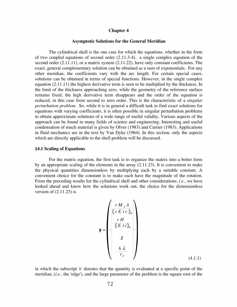
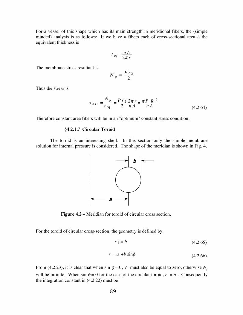
Therefore constant area fibers will be in an "optimum" constant stress condition. §4.2.1.7 Circular Toroid The toroid is an interesting shell. In this section only the simple membrane solution for internal pressure is considered. The shape of the meridian is shown in Fig. 4.

b

a

Figure 4.2 – Meridian for toroid of circular cross section.

For the toroid of circular cross-section, the geometry is defined by: r 1 = b (4.2.65)

r = a +b sinφ (4.2.66) From (4.2.23), it is clear that when sin φ = 0, V must also be equal to zero, otherwise Ns will be infinite. When sin φ = 0 for the case of the circular toroid, r = a . Consequently the integration constant in (4.2.22) must be

90

C = – P a 22 (4.2.67)

Using (4.2.67) and (4.2.22) results in

r V =P

2 r 2 – a 2 (4.2.68)

The membrane solution can now be determined using (4.2.14), (4.2.18), (4.2.65), (4.2.66) and (4.2.68):

N s = V

sinφ = P b r +a r –a

2r r –a = P b

2 1 + ar (4.2.69)

N θ = r 2 P – r 2

r 1 Vsinφ

= r Psinφ

– P r 2 – a 2

2b sin2φ = P b

2 (4.2.70)

Likewise, using (4.2.19) and (4.2.65-68) gives the solution for radial displacement :

hr = P b

2E t 1 –ν 1 +a

r (4.2.71) This membrane solution remains valid at sinφ = 0. The rotation is, from (2.7.3) and (4.2.69-70):

χ sinφ = – dds

r εθ + cosφ ε s

χ sinφ = – 1E t

dds r Nθ– νNs + cosφ Ns –νNθ

χ sinφ = P b

2E t – d

ds r 1 – ν 1 + a r + cosφ 1 + a

r –ν

χ sinφ = P b2E t

a r cosφ

χ = P b2E t

a r cotφ (4.2.72)

Consequently the rotation is singular at φ = 0, π . However, it can be shown that the bending effects correct χ with negligible change in stress in the neighborhood of these singular points. §4.2.2 Axial Load For an axial force:

91

P z ≡ P s ≡ 0 (4.2.73)

r V = F

2 π = C (4.2.74)

The membrane solution consequently is, using (4.2.14, 18) and (4.2.73,74):

N φ = V

sinφ = C

r sinφ (4.2.75)

N s = – r 2

r 1 N φ = – r 2

r 1 Cr sin φ

= – Cr 1 sin2φ (4.2.76)

Using (4.2.19) and (4.2.74) yields the radial displacement:

hr = 1

E t Cr – r 2

r 1 – ν (4.2.77)

h = − CEt sinϕ

r2r1+ ν⎛

⎝⎜⎞⎠⎟ (18oct06)

Using (2.7.3) and (4.2.75,76) provides the result for the rotation:

χ sinφ = – dds

r εθ + cosφ ε s

χ sinφ = 1E t

dds – r Nθ– νNs + cosφ Ns –νNθ

= 1

E t ∂∂s

– r – C r 2

r 1r sinφ – ν C

r sinφ + cosφ C

r sinφ + ν r 2 C

r 1r sinφ

= c E t

– ∂∂s –r 2r 1

1sinφ

+ – r 2r 1

– ν r 2r 1

cosφ

r sinφ +

cosφr sinφ

+ ν r 2 cosφ

r 1r sinφ

= c E t

∂∂s r 2r 1

1sinφ

+ –r 22

r 12cosφ

r sinφ +

cosφr sinφ

χ =

C cosφr E t sin2φ

r cosφ

∂∂s r 2

r 1 + 1 – r 22

r 12 (4.2.78)

92

For the sphere this solution may be shown to be valid at sin φ = 0 ; the singularity corresponds to the concentrated load. For the toroid however, the transverse shear force at φ = 0 must be of a significant magnitude. Thus the singularity of the membrane solution corresponds to a failure of the "membrane" assumption, in the region near sin φ = 0. For the sphere: (18oct06) Ns = C

r sinϕ = −Nθ

v =C 1+ ν( )

Et log tanϕ2⎛⎝⎜

⎞⎠⎟

h = −C 1+ ν( )Et sinϕ

u =C 1+ ν( )

Et − cotϕ + sinϕ log tanϕ2⎛⎝⎜

⎞⎠⎟

w = −C 1+ ν( )

Et 1+ cosϕ log tanϕ2⎛⎝⎜

⎞⎠⎟

χ = 0