Embed Size (px)
Citation preview
ON THE ASYMPTOTIC SOLUTIONS OF ORDINARYDIFFERENTIAL EQUATIONS, WITH AN APPLICATION
TO THE BESSEL FUNCTIONS OF LARGE ORDER*
BY
RUDOLPH E. LANGER
1. Introduction. The investigations which have hitherto been made of
the solutions of the ordinary linear differential equation
(1) u"(x) + p(x)u'(x) + \p2<t>2(x) + q(x)}u(x) = 0,f
with respect to their asymptotic dependence upon the complex parameter p,
have almost without exception been restricted to the case in which <p2(x),
the coefficient of the parameter, remains positive (or negative) over the
entire assigned interval of the variable x. The results in that case are
familiar. Í A determination of coefficients «,-,•(*) in a pair of expressions of
the type
( au(x) au(x) )<r1/2(*)<H1 + -^ + -^ + • • • t '
K p P2 )(2)
( a2i(x) a22(x) ) Ç*d,-v2(x)e-«l 1 + —— + —Li +•■■ \, t=p) <p(x)dx,
is possible, so that the resulting forms represent asymptotically a pair of
solutions of the equation given. Moreover, each of these forms is then known
to represent one and the same solution so long as p remains in a region of
the complex plane in which its pure imaginary part is either invariably
greater than or invariably less than some constant.
The forms (2) are evidently of oscillatory or exponential type according
as <j>2(x) is positive or negative on the x interval under account, and on differ-
ent intervals in which <f>2(x) is of opposite sign the forms are respectively of
the two opposing types. Between two such intervals a change in the charac-
ter of any solution must, therefore, take place. It is evident, however, that
the manner of this change is not deducible from the forms (2), for whatever
the magnitude of p these forms fail to remain significant at a zero of <¡>2(x).
* Presented to the Society, April 18, 1930; received by the editors April 11, 1930.
f It is merely as a matter of convenience that p24?(x) is written rather than fxj>{x).
t Horn, Mathematische Annalen, vol. 52 (1899), pp. 340-362; Birkhoff, these Transactions
vol. 9 (1908), p. 219.
23
License or copyright restrictions may apply to redistribution; see http://www.ams.org/journal-terms-of-use
24 R. E. LANGER [January
Hence there always exists some interval about such a zero in which the forms
do not represent a solution. Because of this failure in the mode of represen-
tation, the relation between the solutions respectively represented by the
forms (2) on opposite sides of a zero of <¡>2{x) is obscured, and the law for
its determination does not appear to have been given. Upon this law de-
pends the complete determination of the form of any specific solution of the
equation in different x intervals.
Directly connected with this problem of the association of solutions repre-
sented by the forms (2) for different values of x, is that of the relation be-
tween the solutions so represented for any fixed value of x but differently
restricted values of p. Indeed, it will be shown that it is a single problem to
determine completely the asymptotic forms in question for unrestricted
values of both x and p. It is this larger problem which is taken as the subject
of the present discussion. It contains the more restricted problems already
mentioned as integral parts, and may perhaps lay claim to some degree of
interest and importance. Aside from its utility as illustrated by the appli-
cation to be discussed below, it may be remarked, in particular, that a solu-
tion of the problem is a requisite to the general extension of the method of
asymptotic forms to the treatment of such boundary problems as result when
an equation of type (1) is subjected to boundary conditions which apply at
points between which 4>2{x) becomes zero.
A special boundary problem of this latter type has on previous occasion*
been considered by the author. While a solution of the general problem de-
scribed above was not found necessary in that case, due to the special
structure of the differential system considered, the discussion and results of
that paper have been largely suggestive for the present considerations. In
this connection it should be noted that the problem at hand as applied to a
specialized equation of the type (1) was raised and briefly discussed by
H. Jeffreysf in 1924, in connection with an application to the solutions of
the Mathieu equation. A resemblance of thought will be noticeable in a
comparison of certain of the considerations of the present paper with those
of the paper cited.
The procedure of the discussion may be briefly outlined as follows. It is
shown to begin with, by the derivation of explicit formulas, that there may
be associated with any given equation of the type (1) a certain "related"
equation. This related equation on the one hand approximates the equation
given in a specific sense and on the other hand is explicitly solvable with the
use of Bessel functions of particular order and argument. It is shown then,
* These Transactions, vol. 31 (1930), pp. 1-24.
t Proceedings of the London Mathematical Society, (2), vol. 23 (1925), p. 428.
License or copyright restrictions may apply to redistribution; see http://www.ams.org/journal-terms-of-use
1931] ASYMPTOTIC SOLUTIONS OF DIFFERENTIAL EQUATIONS 25
at first for restricted values of x and p, and subsequently for general values,
that the solutions of the given equation are represented asymptotically by
the known solutions of the related equation. The asymptotic form so ob-
tained for any particular solution of the equation given is subject to dis-
continuous changes as x passes from one to the other side of a zero of <f>2(x),
or as the value of arg p passes certain specific bounds.* The law which governs
this change is determined and is shown to depend upon the degree to which
<t>2(x) vanishes at the zero under consideration. These deductions occupy
Part I of the paper.
In Part II of the paper the theory of the preceding part is applied to a
special equation which is known to be solved by the Bessel functions of order
p and argument pe. As a result the formulas for the functions J„, Y„ and H„
with arguments p sech a and p sec ß are obtained for all real values of a and ß
and for large positive values of p. These formulas are in the main those
which are familiarly known as representing the functions- in question, and
which are given, for instance, in Watson's treatise. For the so-called inter-
mediate values of the arguments, however, the formulas here obtained show
certain differences and possibly hold certain advantages over those heretofore
given. In any event, it may be not without interest that the various for-
mulas are derived here practically as a group and through the means of a
special application of more or less general results, rather than, as has hereto-
fore been the case, by methods which were especially developed and adapted
to the peculiar ends in view and which vary considerably from one set of
formulas to the next.
Part I
The general theory of the asymptotic forms
2. The given differential equation. A familiar change of dependent vari-
able reduces the equation (1) to the normal form
(3) u"(x) + {pV(*> - x(x)}u(x) = 0,
in which x(x) is a function simply determinable from the coefficients p(x),
and q(x). This form of the equation is conveniently adapted to the consider-
ations which are to be made. The transformation will, therefore, be supposed
to have been carried out, and throughout the discussion the differential equa-
tion will be supposed given in the form (3).
The primary assumption which is to be made, and which principally
* It will be recalled that such changes of asymptotic form occur also in the theory of the Bessel
functions, and that the phenomenon has been designated in that connection as the Stokes' phe-
nomenon.
License or copyright restrictions may apply to redistribution; see http://www.ams.org/journal-terms-of-use
26 R. E. LANGER [January
characterizes the equations to which the discussion is devoted, is that the
interval of the argument x may include a zero of the coefficient 4>2{x). This
and the remaining assumptions are made specific in the following statement
of hypotheses.
(i) The function 4>2{x) vanishes at a point x = x0 to the degree v, where v is
any real positive constant or zero.
(ii) On some interval Ix which contains the point x=x0, the function <j>2{x)
has no zero other than that at x0*
(hi) On some interval I2 which contains the point x=x0, the function
{x—Xo)~"4>2{x) possesses a continuous second derivative and is real and positive
except possibly for a constant complex factor.
(iv) The function x{x) is defined on some interval It which contains the
point x = Xo, and is bounded on any finite portion of this interval.
In the case of any specifically given equation (3) the intervals Ix, I2, and
I3, on which the respective hypotheses above are satisfied, may be finite or
may extend to infinity in either or both directions. Inasmuch as all the
hypotheses are fulfilled only for values of x which are common to all three of
these intervals, the variable x will be taken throughout the following dis-
cussion to lie on an interval I, which is closed at such finite end points as it
may have, which includes the point x=xo, and which contains only points
common to the three intervals Ix, I2, and 73. Subject to these specifications
the sub-intervals into which I is divided by the point x=x0 may be either
finite or infinite.
The hypotheses (i) to (iv) are concerned primarily with the character of
the given equation in the proximity of the point x = x0. In case the interval
I is infinite, it is to be expected that the character of the equation for values
of x remote from x0 is likewise of significance. This is in fact so, and neces-
sitates a further hypothesis which is to be found below in §7.
Neither the. form of the differential equation (3) nor the validity of the
hypotheses made is affected either by the change of independent variable
x' = x—Xo, or by any transfer of a constant factor from the function 4>2{x) to
the parameter p2. Hence it may be assumed without loss of generality, firstly,
that the origin is located at the zero of <j>2{x), i.e., that x0 = 0, and, secondly,
that the function x~v4>2{x) is real and positive.
Since the function x~"<j>2{x) has by hypothesis a continuous second deriva-
tive, an application of Taylor's theorem yields the formula
(4) <i>2{x) = x"{ao + axx + a2{x)x2},
* The case of several, or any number of isolated zeros of 4>2{x) would, of course, be treated by
sub-dividing the interval and considering separately the sub-intervals containing just one zero.
License or copyright restrictions may apply to redistribution; see http://www.ams.org/journal-terms-of-use
1931] ASYMPTOTIC SOLUTIONS OF DIFFERENTIAL EQUATIONS 27
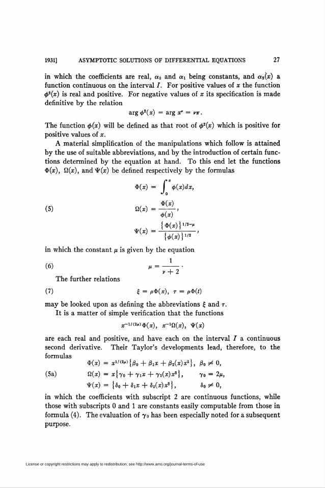
in which the coefficients are real, a0 and <*i being constants, and a2(x) a
function continuous on the interval /. For positive values of x the function
<j>2(x) is real and positive. For negative values of x its specification is made
definitive by the relation
SLTg<t>2(x) = arg x" = vT.
The function <p(x) will be defined as that root of 4>2(x) which is positive for
positive values of x.
A material simplification of the manipulations which follow is attained
by the use of suitable abbreviations, and by the introduction of certain func-
tions determined by the equation at hand. To this end let the functions
<p(#), Q(x), and'í'(x) be defined respectively by the formulas
(5) n(x) =
*(*) =
4>(x) = 4>(x)dx,Jo
$(*)
4>(x)
{#(*)}1/2-
in which the constant p is given by the equation
(6) m =v + 2
The further relations
(7) { = p$(x), r = p*(0
may be looked upon as defining the abbreviations £ and t.
It is a matter of simple verification that the functions
x-l/(2f.)$(x)) ar-lQ(a;)> *(*)
are each real and positive, and have each on the interval / a continuous
second derivative. Their Taylor's developments lead, therefore, to the
formulas*(*) = x^^{ßo + ßiX + ß2(x)x2\, 00^0,
(5a) fí(*) = x{yo + *iix + y2(x)x2}, y0 = 2p,
*(*) = {So + àiX + 52(x)x2}, So^O,
in which the coefficients with subscript 2 are continuous functions, while
those with subscripts 0 and 1 are constants easily computable from those in
formula (4). The evaluation of 70 has been especially noted for a subsequent
purpose.
License or copyright restrictions may apply to redistribution; see http://www.ams.org/journal-terms-of-use
28 R. E. LANGER [January
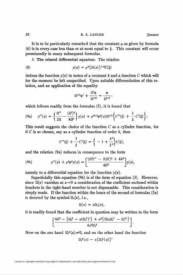
It is to be particularly remarked that the constant p as given by formula
(6) is in every .case less than or at most equal to \. This constant will occur
prominently in many subsequent formulas.
3. The related differential equation. The relation
(8) y{x) =p*{S2(s)}i'2C(S)
defines the function y{x) in terms of a constant k and a function C which will
for the moment be left unspecified. Upon suitable differentiation of this re-
lation, and an application of the equality
fi1'2 O1'2
which follows readily from the formulas (5), it is found that
(9a) /'(*) = |— - -¿)y(x) + p2+ V2(*)n1/2|c"(f) + - c'{Q I.
This result suggests the choice of the function C as a cylinder function, for
if C is so chosen, say as a cylinder function of order k, then
1 ( k2)C"(£)+-C'(£) = | -1+-|C(Ö,
and the relation (9a) reduces in consequence to the form
r(n2)" - 3(ß')2 + 4P-(9b) /'(*) + pWy{x)
r(ii2)" - 3(ß')2 + 4P!= L-ü¡-><*>•namely to a differential equation for the function y{x).
Superficially this equation (9b) is of the form of equation (3). However,
since Q{x) vanishes at x = 0 a consideration of the coefficient enclosed within
brackets in the right-hand member is not dispensable. This consideration is
simply made. If the function within the brace of the second of formulas (5a)
is denoted by the symbol &x{x), i.e.,
ti{x) = xtix{x),
it is readily found that the coefficient in question may be written in the form
T4¿2 - {Oi2 - 3(Ûi2)'} + x2{2ÜxÜ{' - fi/2}'']•
L 4:X2ÜX2
Now on the one hand ux2{x)^0, and on the other hand the function
Í2i2(z)- x\üx2{x)}'
License or copyright restrictions may apply to redistribution; see http://www.ams.org/journal-terms-of-use
1931] ASYMPTOTIC SOLUTIONS OF DIFFERENTIAL EQUATIONS 29
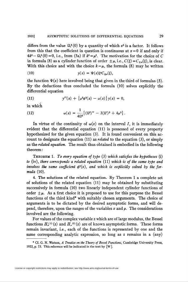
differs from the value ßi2 (0) by a quantity of which x2 is a factor. It follows
from this that the coefficient in question is continuous at x = 0 if and only if
4k2— fíi2(0) =0, i.e., from (5a) if k2=p2. The motivation for the choice of C
in formula (8) as a cylinder function of order ±p, i.e., C(£) =C±(1(£), is clear.
With this choice and with the choice k=p, the formula (8) may be written
(10) y(x) = ♦(aOfrCWÖ,
the function ^(x) here involved being that given in the third of formulas (5).
By the deductions thus concluded the formula (10) solves explicitly the
differential equation
(il) /'(*) + (pV(ï) - «(*)} y(x) = 0,
in which
(12) co(x) = -U(ß2)"-3(fi')2 + V}.40¿
In virtue of the continuity of w(x) on the interval /, it is immediately
evident that the differential equation (11) is possessed of every property
hypothesized for the given equation (3). It is found convenient on this ac-
count to designate the equation (11) as related to the equation (3), or simply
as the related equation. The result thus obtained is embodied in the following
theorem :
Theorem 1. To every equation of type (3) which satisfies the hypotheses (i)
to (iv), there corresponds a related equation (11) which is of the same type and
involves the same coefficient (¡>2(x), and which is explicitly solved by the for-
mula (10).
4. The solutions of the related equation. By Theorem 1 a complete set
of solutions of the related equation (11) may be obtained by substituting
successively in formula (10) two linearly independent cylinder functions of
order ±p. As a first choice it is proposed to use for this purpose the Bessel
functions of the third kind* with suitably chosen arguments. The choice of
arguments is to be dictated by the desired asymptotic forms, and will de-
pend, therefore, upon the ranges of the variables x and p. The considerations
involved are the following.
For values of the complex variable z which are of large modulus, the Bessel
functions fiT„(1) (z) and H¿2) (z) are of known asymptotic forms. These forms
remain invariant, i.e., each of the functions is represented by one and the
same corresponding analytic expression, so long as z remains in a (any)
* Cf. G. N. Watson, A Treatise on the Theory of Bessel Functions, Cambridge University Press,
1922, p. 73. This reference will be indicated in the text by [W].
License or copyright restrictions may apply to redistribution; see http://www.ams.org/journal-terms-of-use
30 R. E. LANGER [January
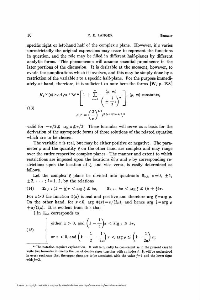
specific right or left-hand half of the complex z plane. However, if z varies
unrestrictedly the original expressions may cease to represent the functions
in question, and the rôle may be filled in different half-planes by different
analytic forms. This phenomenon will assume essential prominence in the
later portions of the discussion. It is desirable at the moment, however, to
evade the complications which it involves, and this may be simply done by a
restriction of the variable z to a specific half-plane. For the purpose immedi-
ately at hand, therefore, it is sufficient to note here the forms [W, p. 198]
£frBW(z)~^^z-1'2e±i2■ - {p,m) -i1+2-1 ~~.-f-;— > Cm» m) constants,
(13)
-K<)"J2\l/2
"-(v) eT0H-l/2)xi/2 *
valid for — 7r/2= arg z^tt/2. These formulas will serve as a basis for the
derivation of the asymptotic forms of those solutions of the related equation
which are to be chosen.
The variable x is real, but may be either positive or negative. The para-
meter p and the quantity £ on the other hand are complex and may range
over the entire respective complex planes. The manner and extent to which
restrictions are imposed upon the locations of x and p by corresponding re-
strictions upon the location of £, and vice versa, is easily determined as
follows.
Let the complex £ plane be divided into quadrants E*,j, k=0, ±1,
±2, • • • ; Z = l, 2, by the relations
(14) H*,i : {k — i)ir < arg £ ^ kv, Ek.i : kv < arg £ = {k + \)v.
For x>0 the function ${x) is real and positive and therefore arg £ = arg p.
On the other hand, for x<0, arg <${x) = v/{2p), and hence arg £ = arg p
-r-ir/(2p). It is evident from this that
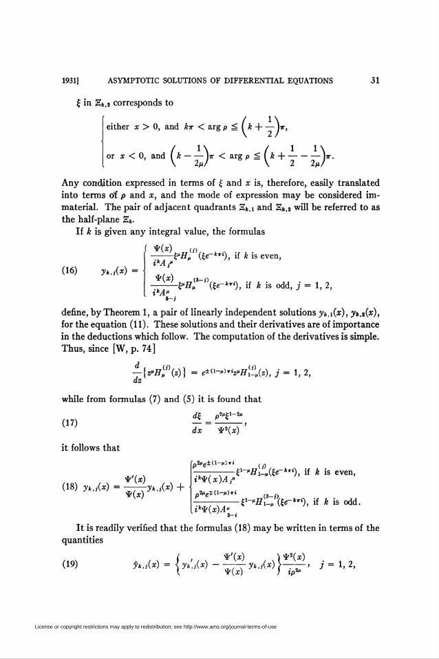
£ in S*,i corresponds to
(15)
either x > 0, and Í k-W < arg p ^ kit,
\ 2 2/J*or x < 0, and I k < arg p «('-¿)';
* The notation requires explanation. It will frequently be convenient as in the present case to
write two formulas in one by the use of double signs together with an index j. It will be understood
in every such case that the upper signs are to be associated with the value /= 1 and the lower signs
with j = 2.
License or copyright restrictions may apply to redistribution; see http://www.ams.org/journal-terms-of-use
1931] ASYMPTOTIC SOLUTIONS OF DIFFERENTIAL EQUATIONS
£ in Et,2 corresponds to
either x > 0, and kir < arg p ^ I k -\-W,
31
or x < 0, and ( k-W < arg p S \ k -\-ta.\ 2pJ \ 2 2M/
Any condition expressed in terms of £ and * is, therefore, easily translated
into terms Of p and x, and the mode of expression may be considered im-
material. The pair of adjacent quadrants St.i and K*,i will be referred to as
the half-plane S*.
If k is given any integral value, the formulas
Í *(*)
(16) yk.j(x) =
,(fl
ikA f
V(x)
í*t1*»-j
£"#„ (£e~*Ti), if * is even,
r(3-j)£"#„ (&-*"), if * is odd, j = 1, 2,
define, by Theorem 1, a pair of linearly independent solutions yk.i(x), yk.2(x),
for the equation (11). These solutions and their derivatives are of importance
in the deductions which follow. The computation of the derivatives is simple.
Thus, since [W, p. 74]
— {«-H^i»} = í*<«^)-VFÍi(«), j = 1, 2,dz
while from formulas (7) and (5) it is found that
d£ p2"£i-2*
(17)
it follows that
(18) ?*.,(*) = —Liy^*) +*(*)
¿x *2(x)
p2/ig±(l-M)l»,(í'
¿^(íc)^/
p2(igi:(l-/i)iri
^^({r»"), if k is even,
[¿^(jc)^"e-^HiJ'^e-""), if ft is odd.
It is readily verified that the formulas (18) may be written in terms of the
quantities
( , *'(*) )^2(x)(19) y~k,,{x) = < yk.j(x) - ——— yk,i(x) >^-—> j = 1, 2,
(. y(x) ) ip2*
License or copyright restrictions may apply to redistribution; see http://www.ams.org/journal-terms-of-use
32 R. E. LANGER [January
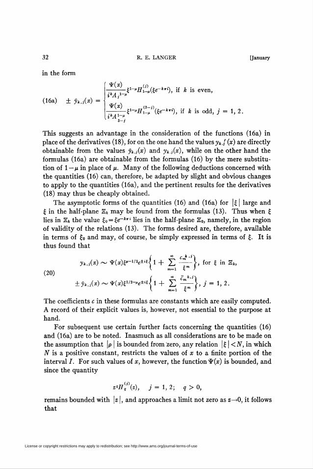
in the form
(16a) ± yk,j{x)
' ^{x) (,)£1-"£Zw(£e-*'i), if k is even,
*(*) (3-3)
£X-"£ZW (V*"), if k is odd, i = 1, 2.UM1-»%-j
This suggests an advantage in the consideration of the functions (16a) in
place of the derivatives (18), for on the one hand the values y*,/ {x) are directly
obtainable from the values yk,j{x) and yk,i{x), while on the other hand the
formulas (16a) are obtainable from the formulas (16) by the mere substitu-
tion of 1 —p in place of p. Many of the following deductions concerned with
the quantities (16) can, therefore, be adapted by slight and obvious changes
to apply to the quantities (16a), and the pertinent results for the derivatives
(18) may thus be cheaply obtained.
The asymptotic forms of the quantities (16) and (16a) for |£| large and
£ in the half-plane E* may be found from the formulas (13). Thus when £
lies in E* the value £0 = £e~*Ti lies in the half-plane So, namely, in the region
of validity of the relations (13). The forms desired are, therefore, available
in terms of £0 and may, of course, be simply expressed in terms of £. It is
thus found that
(20)
ykli{x) ~ ¥(*)e-»*«±«{ 1 + ¿ —\, for £ in E»,I m-l £OT )
±9k,j{x)
£"
*W£i/2-„e±;J1+ ¿ —},/- 1,I m-l £™ )
The coefficients c in these formulas are constants which are easily computed.
A record of their explicit values is, however, not essential to the purpose at
hand.
For subsequent use certain further facts concerning the quantities (16)
and (16a) are to be noted. Inasmuch as all considerations are to be made on
the assumption that \p \ is bounded from zero, any relation |£ | < N, in which
A is a positive constant, restricts the values of x to a finite portion of the
interval /. For such values of x, however, the function1!'^) is bounded, and
since the quantity
z"H^\z), j = 1, 2; q> 0,
remains bounded with \z\, and approaches a limit not zero as z—>0, it follows
that
License or copyright restrictions may apply to redistribution; see http://www.ams.org/journal-terms-of-use
1931] ASYMPTOTIC SOLUTIONS OF DIFFERENTIAL EQUATIONS 33
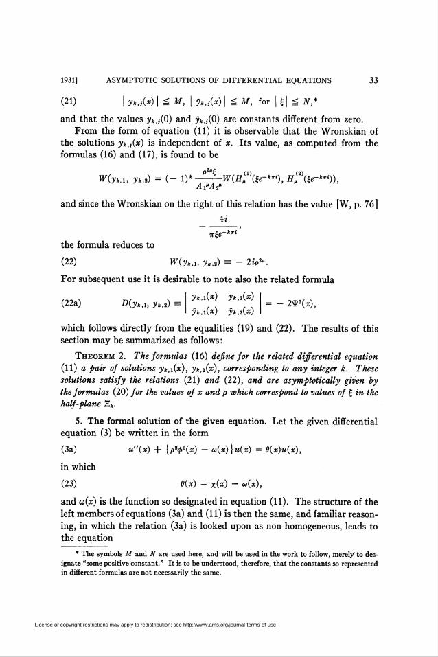
(21) | yk,i(x) | á M, I ?*,,•(*) \úM, for I f I ̂ N*
and that the values y*,,(0) and yt,y(0) are constants different from zero.
From the form of equation (11) it is observable that the Wronskian of
the solutions yk,j(x) is independent of x. Its value, as computed from the
formulas (16) and (17), is found to be
W(yk.i, y*,0 = (- ï)*-f-j-W(H; V*'0, H, V"0),
and since the Wronskian on the right of this relation has the value [W, p. 76]
M
(22a) D(yk.i, y*,i) = - - 2-*2(x),
irle-*"the formula reduces to
(22) W(yk.i, yk,2) - - 2tp2*.
For subsequent use it is desirable to note also the related formula
yk.i(x) yk,i(x)
$k.i(x) yk,i(x)
which follows directly from the equalities (19) and (22). The results of this
section may be summarized as follows:
Theorem 2. The formulas (16) define for the related differential equation
(11) a pair of solutions yt.iOO, yk,2(x), corresponding to any integer k. These
solutions satisfy the relations (21) and (22), and are asymptotically given by
the formulas (20) for the values of x and p which correspond to values of £ in the
half-plane St.
5. The formal solution of the given equation. Let the given differential
equation (3) be written in the form
(3a) u"(x) + \p2<p2(x) - w(x)}u(x) = e(x)u(x),
in which
(23) e(x) = xr» - »(*),
and u(x) is the function so designated in equation (11). The structure of the
left members of equations (3a) and (11) is then the same, and familiar reason-
ing, in which the relation (3a) is looked upon as non-homogeneous, leads to
the equation
* The symbols M and JV are used here, and will be used in the work to follow, merely to des-
ignate "some positive constant." It is to be understood, therefore, that the constants so represented
in different formulas are not necessarily the same.
License or copyright restrictions may apply to redistribution; see http://www.ams.org/journal-terms-of-use
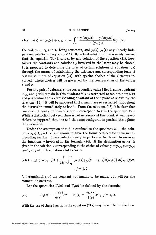
34 R. E. LANGER [January
, s , / N r yi(*)y»W - yMyi{t)(24) u{x) = cxyx{x) + c2y2{x) --8{t)u{t)dt,
J*o W{yx,y2)
the values cx, c2, and xa being constants, and yx{x), y^{x) any linearly inde-
pendent solutions of equation (11). By actual substitution, it is easily verified
that the equation (3a) is solved by any solution of the equation (24), how-
soever the constants and solutions y involved in the latter may be chosen.
It is proposed to determine the form of certain solutions of equation (3a)
through the means of establishing the existence and corresponding form of
certain solutions of equation (24), with specific choices of the elements in-
volved. These choices will be governed by the configuration of the values
x and p.
For any pair of values x, p, the corresponding value £ lies in some quadrant
Sk.i, and £ will remain in this quadrant if x is restricted to maintain its sign
and p is confined to a corresponding quadrant of the p plane as shown by the
relations (15). It will be supposed that x and p are so restricted throughout
the discussion immediately at hand. From the relations (15) it is clear that
two distinct configurations of x and p correspond to £ in the quadrant E&,e
While a distinction between them is not necessary at this point, it will never-
theless be supposed that one and the same configuration persists throughout
the discussion.
Under the assumption that £ is confined to the quadrant Ek,i, the solu-
tions yk,,{x), / = 1, 2, are known to have the forms deduced for them in the
preceding section. These solutions may in particular be chosen to serve as
the functions y involved in the formula (24). If the designation uk,,{x) is
given to the solution u corresponding to the choice of values yx—yk,x, y2 =yk,2,
c, = l, cS-j = 0, the equation (24) becomes
1 rx(24a) uk,j{x) = yk,j{x) + —- I \yk.x{x)yk,2{t) - yk.2{x)yk.i{t)}8{t)uk,i{t)dt,
2ip2"Jxt
j = 1, 2,
A determination of the constant xa remains to be made, but will for the
moment be deferred.
Let the quantities U,{x) and F,(#) be defined by the formulas
Wk.Âx) Vk.Áx)
(25) U¿x) = -VtV^» W = "tTT6™ J=1>2-V{x) ty{x)
With the use of these functions the equation (24a) may be written in the form
License or copyright restrictions may apply to redistribution; see http://www.ams.org/journal-terms-of-use
1931] ASYMPTOTIC SOLUTIONS OF DIFFERENTIAL EQUATIONS 35
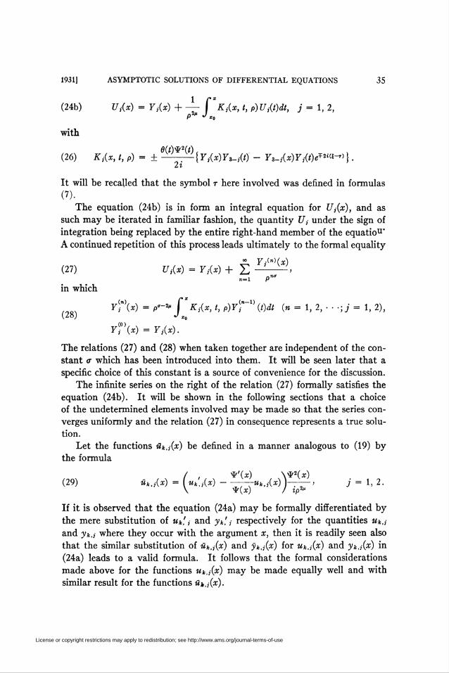
(24b)
with
U,(x) = F,<«) + — (XKi(x, t, p)Uj(t)dt, j = 1, 2,P2" J x0
8(t)¥*(t)(26) Ki(x, t, p) - ± ——-i{ F3(x)F3_i(0 - F3-J-(x)F3(0^2<«-)}.
2t
It will be recalled that the symbol t here involved was defined in formulas
(7).The equation (24b) is in form an integral equation for Uj(x), and as
such may be iterated in familiar fashion, the quantity U,- under the sign of
integration being replaced by the entire right-hand member of the equatiou'
A continued repetition of this process leads ultimately to the formal equality
°° Y ■M(x)(27) U¿x) = Y,ix) + £ -L-L!,
n—1 p
in which
(28)Y?(x) = p-2» C*KAx, t, p)Y(; "(t)dt (n - 1, 2, • ■ -;j = 1, 2),
F^x) = F,(x).
The relations (27) and (28) when taken together are independent of the con-
stant o- which has been introduced into them. It will be seen later that a
specific choice of this constant is a source of convenience for the discussion.
The infinite series on the right of the relation (27) formally satisfies the
equation (24b). It will be shown in the following sections that a choice
of the undetermined elements involved may be made so that the series con-
verges uniformly and the relation (27) in consequence represents a true solu-
tion.
Let the functions üktj(x) be defined in a manner analogous to (19) by
the formula
/ , *'(*) \^2(x)(29) ûk.i(x) = I uk,j(x)-T—uk,j(x) J——— j / = 1, 2.
\ V(x) I ip2"
If it is observed that the equation (24a) may be formally differentiated by
the mere substitution of wt'j and yk!¡ respectively for the quantities ukij
and yk,j where they occur with the argument x, then it is readily seen also
that the similar substitution of «*,,■(*) and yk,,-(x) for uktj(x) and yk.i(x) in
(24a) leads to a valid formula. It follows that the formal considerations
made above for the functions ukij(x) may be made equally well and with
similar result for the functions w*,,(x).
License or copyright restrictions may apply to redistribution; see http://www.ams.org/journal-terms-of-use
36 R. E. LANGER [January
6. Lemmas. The proof of the existence of a set of solutions U¡(x) of
equation (24b), and the associated investigation of their structure, is to be
based upon the relation (27) obtained formally in §5. It is requisite to this
end that the infinite series involved in the relation be shown convergent.
This is conveniently done by means of the facts which are framed below in
the form of a set of simple lemmas.
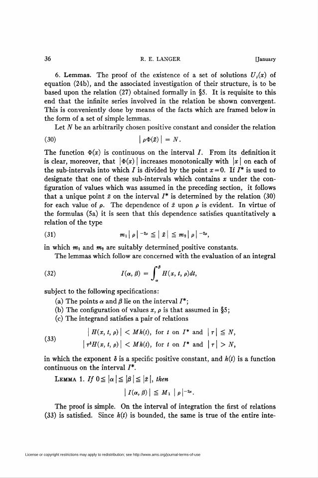
Let N be an arbitrarily chosen positive constant and consider the relation
(30) | p$(x) | = N.
The function $(#) is continuous on the interval I. From its definition it
is clear, moreover, that |$(x) | increases monotonically with \x | on each of
the sub-intervals into which / is divided by the point x = 0. If I* is used to
designate that one of these sub-intervals which contains x under the con-
figuration of values which was assumed in the preceding section, it follows
that a unique point x on the interval 7* is determined by the relation (30)
for each value of p. The dependence of x upon p is evident. In virtue of
the formulas (5a) it is seen that this dependence satisfies quantitatively a
relation of the type
(31) mi\ p\ ~2" = | x\ á í»í|p|-^,
in which Wi and nh are suitably determined^ positive constants.
The lemmas which follow are concerned with the evaluation of an integral
(32) I(a, ß) = H(x, t, p)dt,J a
subject to the following specifications:
(a) The points a and ß lie on the interval /*;
(b) The configuration of values x, p is that assumed in §5 ;
(c) The integrand satisfies a pair of relations
I H(x, t,p)\ < Mh(t), for t on I* and I r I = N,(33)
| tsH(x, t,p)\ < Mh(t), for t on I* and \t\> N,
in which the exponent 5 is a specific positive constant, and h(l) is a function
continuous on the interval I*.
Lemma 1. If 0 = |a | = \ß | = \x \, then
\l(a,ß)\ = Mi |p|-2".
The proof is simple. On the interval of integration the first of relations
(33) is satisfied. Since h(t) is bounded, the same is true of the entire inte-
License or copyright restrictions may apply to redistribution; see http://www.ams.org/journal-terms-of-use
1931] ASYMPTOTIC SOLUTIONS OF DIFFERENTIAL EQUATIONS 37
grand, and by relation (31) the length of the interval of integration is of the
order of \p |-2*.
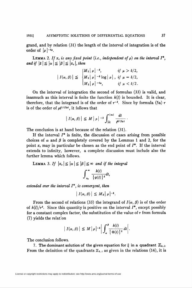
Lemma 2. // xc is any fixed point {i.e., independent of p) on the interval I*,
andif \x\^\a\^\ß\e\xc \, then
/(«, ß) | ^
M2\p\ -*, if p> S/2,
JW21 P 1 -Mog | p | , if p = 0/2,
M2\p\ ~2", if p < 5/2.
On the interval of integration the second of formulas (33) is valid, and
inasmuch as this interval is finite the function h{t) is bounded. It is clear,
therefore, that the integrand is of the order of t~K Since by formula (5a) t
is of the order of ptl"-2l,), it follows that
I{a, ß) | è M I p | -« fJ\~>
i*i dt
ft <«/<2")
The conclusion is at hand because of the relation (31).
If the interval /* is finite, the discussion of cases arising from possible
choices of a and ß is completely covered by the Lemmas 1 and 2, for the
point xc may in particular be chosen as the end point of /*. If the interval
extends to infinity, however, a complete discussion must include also the
further lemma which follows.
Lemma 3. If \xc \ = \a | = |/3 | = °o and if the integral
h{t)
f•J T..
-dt,
extended over the interval I*, is convergent, then
\l{a,ß)\ =M3|p|-{.
From the second of relations {33) the integrand of I{a, ß) is of the order
of h{t)/rs. Since this quantity is positive on the interval /*, except possibly
for a constant complex factor, the substitution of the value of t from formula
(7) yields the relation
h{t)I{a,ß)\ = M\p\-> ..„¡.dthl f-1 \í{ Ht)
The conclusion follows.
7. The dominant solution of the given equation for £ in a quadrant E*,¿.
From the definition of the quadrants Eam as given in the relations (14), it is
License or copyright restrictions may apply to redistribution; see http://www.ams.org/journal-terms-of-use
38 R. E. LANGER [January
directly evident that when £ remains on such a quadrant the real part of ¿£
is either always positive oral ways negative. Hence one and the same one of
the two solutions yt,,(x) remains dominant for all such values of £. Whether
the subscript value associated with this dominant solution is/ = l, or/= 2,
will depend, of course, upon the particular quadrant St.¡ under considera-
tion, namely, upon the values k and /. To avoid an unessential differentiation
of cases the value/ in question will be designated simply by/=/'.
The subject of immediate attention in the present section is the deriva-
tion of a solution of the equation (24b) from the relation (27) for the value
/=/'. This involves a determination of the conditions under which the rela-
tion is convergent, and centers, therefore, upon a consideration of the
quantities Y¡"\x) defined by the formula (28).
The constant x0 was introduced into the formulas of §5, but was referred
for later specification. This specification for the case in hand will now be
made as follows, namely, when j=j', then xQ = 0. It will be understood
throughout this section that this value of x0 has been fixed upon, and it will
be understood likewise without repeated specific mention of the fact that j
temporarily takes the single value /' in the various formulas to be written.
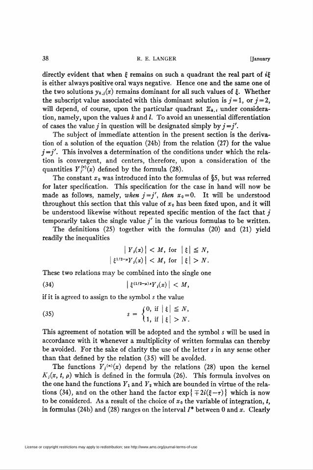
The definitions (25) together with the formulas (20) and (21) yield
readily the inequalities
| Y,(x) | < M, for | £ | á N,
\t.w-"Yj(x)\ <M,ior \t\>N.
These two relations may be combined into the single one
(34) | £«'*-*>»F,(aÛ | < M,
if it is agreed to assign to the symbol s the value
0, if | £ | á N,
1, if |f| > N.
This agreement of notation will be adopted and the symbol s will be used in
accordance with it whenever a multiplicity of written formulas can thereby
be avoided. For the sake of clarity the use of the letter s in any sense other
than that defined by the relation (35) will be avoided.
The functions F/n)(x) depend by the relations (28) upon the kernel
Kj(x, t, p) which is defined in the formula (26). This formula involves on
the one hand the functions Yi and F2 which are bounded in virtue of the rela-
tions (34), and on the other hand the factor exp{ + 2¿(£ — t)\ which is now
to be considered. As a result of the choice of x0 the variable of integration, /,
in formulas (24b) and (28) ranges on the interval I* between 0 and x. Clearly
(35) s =
License or copyright restrictions may apply to redistribution; see http://www.ams.org/journal-terms-of-use
1931] ASYMPTOTIC SOLUTIONS OF DIFFERENTIAL EQUATIONS 39
then |t I = |£ |. Since the value arg t is constant on the interval /* it follows
that for the values of t in hand
arg [i(£ - t)] = arg i£.
The exponent + 2¿(£ — t) in formula (26) is, therefore, of real part opposite
in sign to that of the corresponding exponent in the formula (20). Inasmuch
as the latter is positive for j =j', in virtue of the determination of j', the
exponential in K¡{x, t, p) is bounded when \t\ does not exceed |*|. This
conclusion, together with the inequalities (34), establishes, for |z | = \x |, the
relations
I P'^'K^x, t,p)\ = M*2{t) | 0(Z) | , for | r | = N,(36) , , i i i i
| r(i/2-,)^i/2-,).jç.(X) /( p) I = MW{t) | 8{t) | , for | r | > A7.
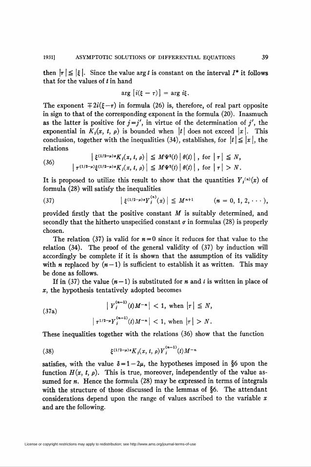
It is proposed to utilize this result to show that the quantities Y/n){x) of
formula (28) will satisfy the inequalities
(37) | ^i2-^'Y{"\x) | = M"+1 {n = 0, 1, 2, • • • ),
provided firstly that the positive constant M is suitably determined, and
secondly that the hitherto unspecified constant <r in formulas (28) is properly
chosen.
The relation (37) is valid for « = 0 since it reduces for that value to the
relation (34). The proof of the general validity of (37) by induction will
accordingly be complete if it is shown that the assumption of its validity
with n replaced by (« — 1) is sufficient to establish it as written. This may
be done as follows.
If in (37) the value {n — 1) is substituted for n and / is written in place of
x, the hypothesis tentatively adopted becomes
| Y{r1\t)M~n\ < 1, when \t\ UN,(37a)
| T1/2-*F-"_1)(0-M"-n| < 1, when \t\ > N.
These inequalities together with the relations (36) show that the function
(38) ^i2-rt°K¡{x, t, p)Y{rl\t)M-n
satisfies, with the value 5 = 1 — 2p, the hypotheses imposed in §6 upon the
function H{x, t, p). This is true, moreover, independently of the value as-
sumed for n. Hence the formula (28) may be expressed in terms of integrals
with the structure of those discussed in the lemmas of §6. The attendant
considerations depend upon the range of values ascribed to the variable x
and are the following.
License or copyright restrictions may apply to redistribution; see http://www.ams.org/journal-terms-of-use
40 R. E. LANGER [January
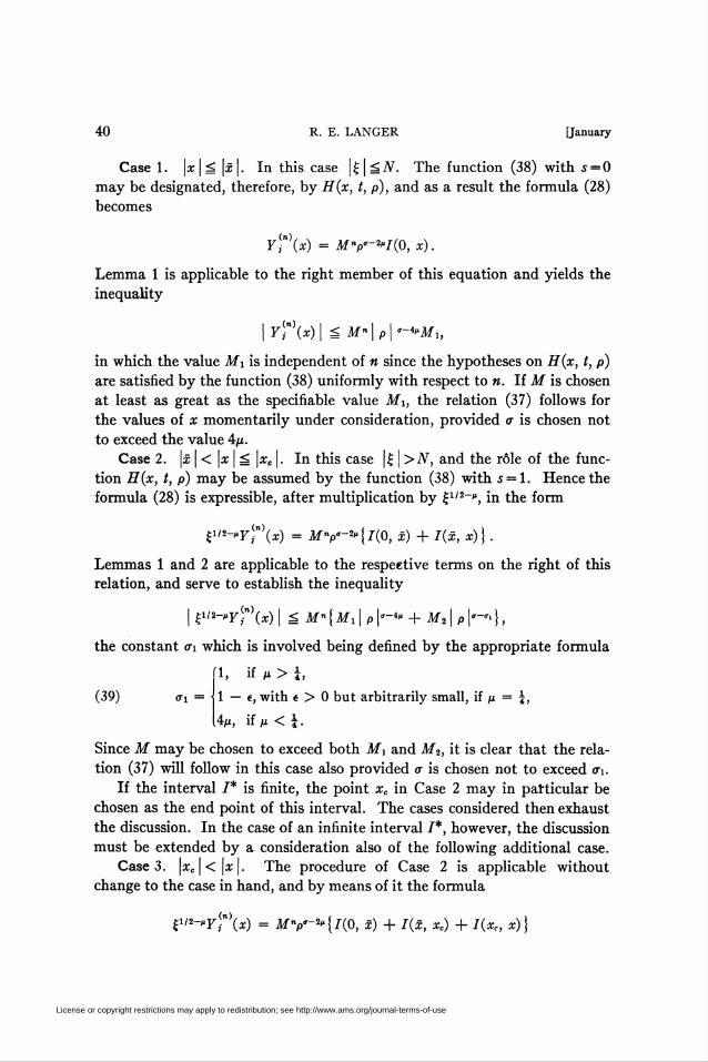
Case 1. |x|= |x|. In this case \è\^N. The function (38) with s = 0
may be designated, therefore, by H(x, t, p), and as a result the formula (28)
becomes
F -n)(x) = M»p'-2"/(0, x).
Lemma 1 is applicable to the right member of this equation and yields the
inequality
| F?\x) | = M" | p | '-'"Mi,
in which the value Mi is independent of n since the hypotheses on H(x, t, p)
are satisfied by the function (38) uniformly with respect to n. If M is chosen
at least as great as the specifiable value Mh the relation (37) follows for
the values of x momentarily under consideration, provided a is chosen not
to exceed the value 4p.
Case 2. \x \ < \x | = |ícc |. In this case |£ | >N, and the rôle of the func-
tion H(x, t, p) may be assumed by the function (38) with s = l. Hence the
formula (28) is expressible, after multiplication by £1/2_", in the form
el2-"Yt\x) = M"p'-2"{l(0, x) + I(x, x)).
Lemmas 1 and 2 are applicable to the respective terms on the right of this
relation, and serve to establish the inequality
| £1'2-"F ■"'(*) | = M" {Mi | p |"-4" + M2\p |"-"'},
the constant en which is involved being defined by the appropriate formula
1, if p > {,
(39) <xi = • 1 — €, with e > 0 but arbitrarily small, if p = \,
4p, if m < ï •
Since M may be chosen to exceed both Mj and M2, it is clear that the rela-
tion (37) will follow in this case also provided cr is chosen not to exceed tri.
If the interval I* is finite, the point xe in Case 2 may in patticular be
chosen as the end point of this interval. The cases considered then exhaust
the discussion. In the case of an infinite interval /*, however, the discussion
must be extended by a consideration also of the following additional case.
Case 3. |*c|<|a:|. The procedure of Case 2 is applicable without
change to the case in hand, and by means of it the formula
£1'2-"F,-n)(x) = My-"{/(0, x) + I(x, xc) + I(xc, *)}
License or copyright restrictions may apply to redistribution; see http://www.ams.org/journal-terms-of-use
1931] ASYMPTOTIC SOLUTIONS OF DIFFERENTIAL EQUATIONS 41
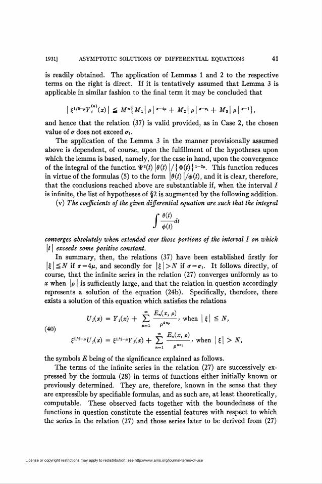
is readily obtained. The application of Lemmas 1 and 2 to the respective
terms on the right is direct. If it is tentatively assumed that Lemma 3 is
applicable in similar fashion to the final term it may be concluded that
| £i/2-«Ff\») | = M"{ Mx | p | '-<» + M21 p | "-*> + M31 p | '-1},
and hence that the relation (37) is valid provided, as in Case 2, the chosen
value of <r does not exceed <rx.
The application of the Lemma 3 in the manner provisionally assumed
above is dependent, of course, upon the fulfillment of the hypotheses upon
which the lemma is based, namely, for the case in hand, upon the convergence
of the integral of the function *2(Z) \8{t) \/ {$(i)}l-*». This function reduces
in virtue of the formulas (5) to the form \8{t) \/<f>{t), and it is clear, therefore,
that the conclusions reached above are substantiable if, when the interval /
is infinite, the list of hypotheses of §2 is augmented by the following addition.
(v) The coefficients of the given differential equation are such that the integral
Ie{t) J-dt<b{t)
converges absolutely when extended over those portions of the interval I on which
\t | exceeds some positive constant.
In summary, then, the relations (37) have been established firstly for
| £ | S N if <r = 4p, and secondly for | £ | > N if <r = <rx. It follows directly, of
course, that the infinite series in the relation (27) converges uniformly as to
x when \p | is sufficiently large, and that the relation in question accordingly
represents a solution of the equation (24b). Specifically, therefore, there
exists a solution of this equation which satisfies the relations
Uj(x) = Y Ax) + ¿ EÁ*'p), when \i\úN,(40) n=1 j"
^-"U^x) = e'^Y^x) + ¿ » when I £l > N,n=l P""
the symbols E being of the significance explained as follows.
The terms of the infinite series in the relation (27) are successively ex-
pressed by the formula (28) in terms of functions either initially known or
previously determined. They are, therefore, known in the sense that they
are expressible by specifiable formulas, and as such are, at least theoretically,
computable. These observed facts together with the boundedness of the
functions in question constitute the essential features with respect to which
the series in the relation (27) and those series later to be derived from (27)
License or copyright restrictions may apply to redistribution; see http://www.ams.org/journal-terms-of-use
42 R. E. LANGER [January
are of interest from the viewpoint of the discussion of the present paper. An
economy of thought and formulas may, therefore, be achieved by the use of
the letter £ as a generic symbol in the following sense. The symbol E shall
designate merely some computable function which is bounded for the ranges
of its arguments under consideration. In a given formula different functions
E will be distinguished by the use of subscripts. There is to be no presump-
tion, however, that the same symbol in different formulas designates the
same function. As a case in point it is evident that the functions similarly
designated in the two equations (40) are not the same.
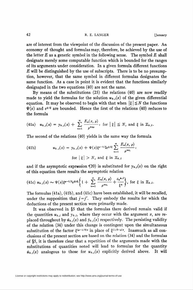
By means of the substitutions (25) the relations (40) are now readily
made to yield the formulas for the solution uk.i(x) of the given differential
equation. It may be observed to begin with that when |£ | = iV the functions
ty(x) and e±,f are bounded. Hence the first of the relations (40) reduces to
the formula
* En(x, p) . .(41a) ukij(x) = yt.,(x) + £-> for £ = N, and £ in St.j.
n-l P4n"
The second of the relations (40) yields in the same way the formula
" En(x, p)(41b) Ukj(x) = y4i/(*) + *(x)£*-i/2e±i£ £ -— >
n=l P"'1
for | £| > N, and £ in St,¡
and if the asymptotic expression -(20) is substituted for yk,¡(x) on the right
of this equation there results the asymptotic relation
(41c) uk,i(x) ~*(x)?-ll2e±il{l + £ " *' P + — \, for £ in S*.i.I n=i p™1 £n ;
The formulas (41a), (41b), and (41c) have been established, it will be recalled,
under the supposition that/=/'. They embody the results for which the
deductions of the present section were primarily made.
It was observed in §5 that the formulas there derived remain valid if
the quantities uk,j and yk,¡, where they occur with the argument x, are re-
placed throughout by ük,i(x) and yt,j(x) respectively. The persisting validity
of the relation (34) under this change is contingent upon the simultaneous
substitution of the factor £("-1'2>s in place of £0/2-11)«. Inasmuch as all con-
clusions of the present section are based on the relation (34) and the formulas
of §5, it is therefore clear that a repetition of the arguments made with the
substitutions of quantities noted will lead to formulas for the quantity
uk,j(x) analogous to those for wt,,(x) explicitly derived above. It will
License or copyright restrictions may apply to redistribution; see http://www.ams.org/journal-terms-of-use
1931] ASYMPTOTIC SOLUTIONS OF DIFFERENTIAL EQUATIONS 43
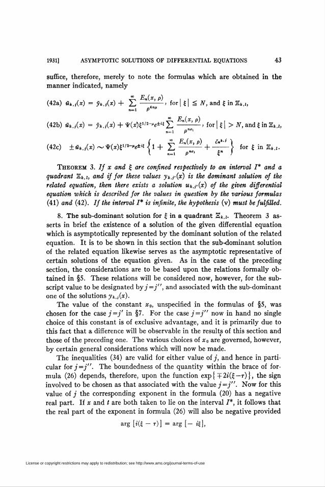
suffice, therefore, merely to note the formulas which are obtained in the
manner indicated, namely
o» En{x p)
(42a) «».,(*) = yk.i{x) + £ " ' > for | £ | = N, and £ in St.i,n-l P4""
» E {x p)(42b) «».,-(*) = ykti{x)+^{x)el2-"e^2Z " ' > for | f | > JV, and£inE*,¡,
n_l Pn"
(42c) ± **.,(*) ~ *(*)£1/2-»e±i{ < 1 + £ —^-^ +-\ for £ in 8».i.I „=i Pn" £n j
Theorem 3. If x and £ ore confined respectively to an interval I* and a
quadrant 8»,i, and if for these values yk.r{x) is the dominant solution of the
related equation, then there exists a solution uktj>{x) of the given differential
equation which is described for the values in question by the various formulas
(41) and (42). If the interval I* is infinite, the hypothesis (v) must be fulfilled.
8. The sub-dominant solution for £ in a quadrant E*,z. Theorem 3 as-
serts in brief the existence of a solution of the given differential equation
which is asymptotically represented by the dominant solution of the related
equation. It is to be shown in this section that the sub-dominant solution
of the related equation likewise serves as the asymptotic representative of
certain solutions of the equation given. As in the case of the preceding
section, the considerations are to be based upon the relations formally ob-
tained in §5. These relations will be considered now, however, for the sub-
script value to be designated by j=j", and associated with the sub-dominant
one of the solutions yk,¡{x).
The value of the constant x0, unspecified in the formulas of §5, was
chosen for the case /=/' in §7. For the case j=j" now in hand no single
choice of this constant is of exclusive advantage, and it is primarily due to
this fact that a difference will be observable in the results of this section and
those of the preceding one. The various choices of x0 are governed, however,
by certain general considerations which will now be made.
The inequalities (34) are valid for either value of /, and hence in parti-
cular for j—j". The boundedness of the quantity within the brace of for-
mula (26) depends, therefore, upon the function exp{ +2i(£—t)}, the sign
involved to be chosen as that associated with the value j=j". Now for this
value of j the corresponding exponent in the formula (20) has a negative
real part. If x and / are both taken to lie on the interval /*, it follows that
the real part of the exponent in formula (26) will also be negative provided
arg [i(£ - t)] = arg [- i£],
License or copyright restrictions may apply to redistribution; see http://www.ams.org/journal-terms-of-use
44 R. E. LANGER [January
a condition which is fulfilled if and only if |t | = |£ |, i.e., if \t | — \x |. Inas-
much as the variable of integration t in formulas (24b) and (28) ranges over
the interval bounded by x and x0, it is clear that when x0 is chosen the con-
siderations must be confined to those values of x on the interval I* for which
0= \x | = |*o |. With this restriction the inequalities (36) are readily found
to be valid for j—j" provided \t\= \x \.
With any choice of x0 on the interval /*, and x restricted as determined
above, it follows from the assumption (37a), as in the preceding section,
that the function (38) satisfies the hypotheses imposed in §6 upon the func-
tion H(x, t, p). Hence the expression of the formula (28) by means of integrals
with the structure of those considered in the lemmas of §6 is possible, and
with appropriate choices of the value a the relations (37) may be established
as follows.
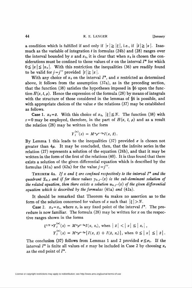
Case 1. x0=x. With this choice of x0, |£ | =iV. The function (38) with
s = 0 may be employed, therefore, in the part of H(x, t, p) and as a result
the relation (28) may be written in the form
F-"'(x) = Mnp"-2"I(x, x).
By Lemma 1 this leads to the inequalities (37) provided cr is chosen not
greater than 4p. It may be concluded, then, that the infinite series in the
relation (27) represents a solution of the equation (24b), and that it may be
written in the form of the first of the relations (40). It is thus found that there
exists a solution of the given differential equation which is described by the
formulas (41a) and (42a) for the value/=/".
Theorem 4a. If x and £ are confined respectively to the interval I* and the
quadrant Et,¡ and if for these values yk,,"(x) is the sub-dominant solution of
the related equation, then there exists a solution uk,j"(x) of the given differential
equation which is described by the formulas (41a) and (42 a).
It should be remarked that Theorem 4a makes no assertion as to the
form of the solution concerned for values of x such that | £ | > N.
Case 2. x0 = xc, where xc is any fixed point of the interval I*. The pro-
cedure is now familiar. The formula (28) may be written for x on the respec-
tive ranges shown in the forms
£1/2-"F,n)(x) = Mnp°-2»I(x, xc), when | x\ < | x| = | xc \ ,
Y<¡n\x) = Mnp°-2"{l(x, x) + I(x, xc)}, when 0 ^ | x| = \ x\ .
The conclusion (37) follows from Lemmas 1 and 2 provided a¿ai. If the
interval I* is finite all values of x may be included in Case 2 by choosing xe
as the end point of I*.
License or copyright restrictions may apply to redistribution; see http://www.ams.org/journal-terms-of-use
1931] ASYMPTOTIC SOLUTIONS OF DIFFERENTIAL EQUATIONS 45
It is to be especially noted that by formula (28) the quantities Yj^(-n){x)
are essentially dependent upon the value x0, and that these quantities in
Case 2 are, therefore, not identical with those in Case 1. Despite this fact it
will not be found necessary to resort to a distinguishing notation for the
solutions concerned in the respective cases.
If the interval 7* is infinite, it will be supposed as in §7 that the hypothesis
(v) is fulfilled. The considerations may be extended, then, also to the
following case.
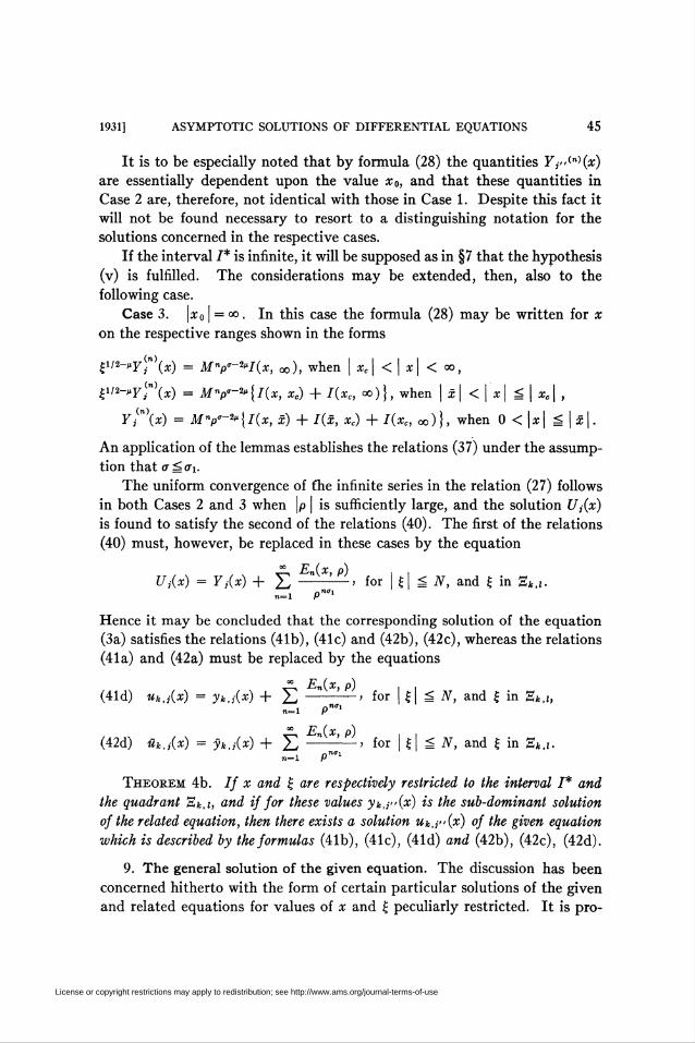
Case 3. \xQ | = <x>. In this case the formula (28) may be written for x
on the respective ranges shown in the forms
£1'2-"FJn {x) = Mnp"-2"I{x, oo ), when | xc \ < | x \ < <x>,
£1/2-*FJn)(x) = Mnp'-2"{l{x, xc) + I{xc, <»)}, when \x\ < \ x | g | xc\ ,
Y,M{x) = M"p'-2"{l{x, x) + I{x, xc) + I{xc, «))}, when 0 < |*| á |«|.
An application of the lemmas establishes the relations (37) under the assump-
tion that a = ax.
The uniform convergence of the infinite series in the relation (27) follows
in both Cases 2 and 3 when \p | is sufficiently large, and the solution U,{x)
is found to satisfy the second of the relations (40). The first of the relations
(40) must, however, be replaced in these cases by the equation
" En{x, p) . .U,{x) = Yj{x) + 2Z -' for £ = N, and £ in E*,¡.
„=i p"i
Hence it may be concluded that the corresponding solution of the equation
(3a) satisfies the relations (41b), (41c) and (42b), (42c), whereas the relations
(41a) and (42a) must be replaced by the equations
» En{x p)(41d) uk,j{x) = yk,j{x) + £ " ' ■ > for | £| = N, and £ in E4,i,
n=l Pn°l
" En{x, p) . ,(42d) ükij{x) = yk,j{x) + ¿_, -' for £ = iV, and £ in E*,¡.
n=l P
Theorem 4b. If x and £ are respectively restricted to the interval I* and
the quadrant S»,j, and if for these values yk,¡"{x) is the sub-dominant solution
of the related equation, then there exists a solution uk,j"{x) of the given equation
which is described by the formulas (41b), (41c), (41d) and (42b), (42c), (42d).
9. The general solution of the given equation. The discussion has been
concerned hitherto with the form of certain particular solutions of the given
and related equations for values of x and £ peculiarly restricted. It is pro-
License or copyright restrictions may apply to redistribution; see http://www.ams.org/journal-terms-of-use
46 R. E. LANGER [January
posed now to extend the considerations to the general solutions of these
equations and to general values of the parameter and variable.
In the foregoing sections it was convenient to base the deductions upon
the particular sets of solutions yt,,-(x), because of the especial simplicity
of the corresponding asymptotic forms for the values of £ on the restricted
ranges considered. The advantage in this choice naturally fails to persist
when general values of £ are drawn into account.. It is for this reason con-
venient to introduce at this point as a basis for the continuing discussion a
set of solutions distinct from any of those hitherto used. These solutions
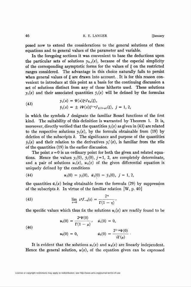
yi(x) and their associated quantities y¡(x) will be defined by the formulas
yÁx) - *(*)£"/*„(£),(43)
y,(x) = ± ¿*(x)£1-"/±(1_,,(£), j = 1, 2,
in which the symbols / designate the familiar Bessel functions of the first
kind. The suitability of this definition is warranted by Theorem 1. It is,
moreover, directly verified that the quantities y¡(x) as given in (43) are related
to the respective solutions y¡(x), by the formula obtainable from (19) by
deletion of the subscripts k. The significance and purpose of the quantities
y¡(x) and their relation to the derivatives yf (x), is familiar from the rôle
of the quantities (19) in the earlier discussion.
The point x = 0 is an ordinary point for both the given and related equa-
tions. Hence the values y,(0), y,(0),/ = l, 2, are completely determinate,
and a pair of solutions ui(x), u2(x) of the given differential equation is
uniquely defined by the conditions
(44) «,(0) = yAO), *,(0) = y,(0), j = 1, 2,
the quantities w,(x) being obtainable from the formula (29) by suppression
of the subscripts k. In virtue of the familiar relation [W, p. 40J
2"(45) lim z"J-,(z) =
«-o T(l - r,)
the specific values which thus fix the solutions «,■(*) are readily found to be
2*¥(0)«i(0)=—--> «i(0)=0,
(46) r(1 - M)
21"*¥(0)«2(0) = 0, *,(0) = ——— •
iT(p)
It is evident that the solutions ui(x) and u2(x) are linearly independent.
Hence the general solution, u(x), of the equation given can be expressed
License or copyright restrictions may apply to redistribution; see http://www.ams.org/journal-terms-of-use
1931] ASYMPTOTIC SOLUTIONS OF DIFFERENTIAL EQUATIONS 47
linearly in terms of them. The explicit formula is in fact easily obtained,
and is the following: if the solution u{x) takes at x = 0 the values
(47a) «(0) = C, «(0) = C,
thenr(i - p)c ir{p)c
(47b) u{x) =-ux{x) H-u2{x).2"*(0) 21-»*(0)
With the formula (47b) at hand it is clear that a determination of form for
the solutions ux{x) and u2{x) suffices in every respect for a corresponding
determination of form for the general solution of the equation given.
Let any value x on the interval I be chosen, and letp be located at pleasure
in the complex plane subject to the condition that \p | be sufficiently large.
The corresponding value of £ lies in some one of the quadrants (14), and the
designation of this quadrant by Et,» has merely the significance of an assign-
ment of values to k and /. For the value of k thus fixed upon and for the
value of £ in question the solutions uk,,{x) given by the Theorems 3 and
either 4a, or 4b, have the forms respectively deduced for them in §§7, and 8,
and are given accordingly by the appropriate formulas (41) and (42). Be-
tween any pair of these solutions and the solutions u¡{x) considered above
there exists, of course, a set of identical relations
i \ <*> i \ i {k) i \ui{x) = ai,xuktX{x) + ai,2uk,2{x),
(48a) (*) (t)ûi(x) = altXük,x{x) + ai,2üki2{x), I = 1, 2,
with coefficients at,j(h) which are free from x but which naturally depend
upon the solutions uk,,{x) involved. The existence of an analogous set of
relations involving the corresponding solutions of the related equation, i.e.,
r \ (k) i \ i (*> i \yi(x) = ci,xyk,x{x) + cil2ykl2{x),
(48b) - f \ (*> - f \ _l_ (t) - f \ 7 10yi{x) = ci,xyk,x{x) + ctl2yk,2{x), I => 1, 2,
is evident.
The coefficients in the identities (48a) and (48b) are easily calculated
by setting x = 0 and solving the resulting system of algebraic equations. In
virtue of the relations (44) the resulting values may be written
(*) + {y«(0)fl*./(0) - yi{0)uk,¡{0)\(49a) di.i-j =-'
D{uk,x{0), uk,2{0))
(*) + {yi{0)yk.A0) - yi{0)yk,i{0)} . , .(49b) C',3-i =-■> j = 1,2,
D{yk.x{0),yk.2{0))
License or copyright restrictions may apply to redistribution; see http://www.ams.org/journal-terms-of-use
48 R. E. LANGER [January
the symbol D having the significance given it in formula (22a). The evident
similarity of structure of the right hand members of formulas (49a) and (49b)
will be used as a basis for deducing also a similarity of values of the coeffi-
cients which they represent.
Let the attention be given first to a consideration of those values of x
and p for which |£ | =iV. The solutions uk,j(x) in formulas (48a) and (49a)
are in this case conveniently taken as those described by the Theorems 3
and 4a. The formulas (41a) and (42a) may accordingly be drawn upon for
an evaluation of the quantities ukij(0) and «t,j(0), and if these values are
substituted into the relations (49a) and the resulting formulas are compared
with the relations (49b), it is found that
(*) c*> A En(p)ai.i = cu + 2-j —;—> J> * = !j 2.
n=l P
With these coefficient values, and with the values of uk,j(x) and ük,j(x) given
by the formulas (41a) and (42a), the identities (48a) are found upon com-
parison with (48b) to reduce to the form
ui(x) = yi(x) + £En(x, p)
p4n"
" EJx, p)m(x) = yt(x)+ £ =ÍLU1, 1-1, 2.
»-1 P4""
Inasmuch as the quantities y in these equations are those of the formulas
(43), the results obtained may be summarized as follows:
Theorem 5. The solutions ui(x), u2(x), of the given differential equation,
which at x = 0 take on the values (46), are described by the formulas
A En(x, p)«,(*) = *(x)£x/T„(£) + £ —Li^i,
n-l P
A En(x, p)a¿x) = ± mx)e-"J±a-AÛ + £ —-—- j = 1, 2,
n=l P
for all values of x and p subject to the relation |£ | = N.
Let the attention be turned now to a consideration of the values of x and
p for which |£ | >iV. The procedure to be followed is in its initial stage similar
to that followed above, with the difference, however, that the solutions
Uk,i(x) involved in the formulas (48a) and (49a) are to be looked upon as
those given by the Theorems 3 and 4b rather than by Theorems 3 and 4a as
heretofore. This change in the point of view is seen directly to be permissible,
License or copyright restrictions may apply to redistribution; see http://www.ams.org/journal-terms-of-use
1931] ASYMPTOTIC SOLUTIONS OF DIFFERENTIAL EQUATIONS 49
for the solutions on the left of the identities (48a) are uniquely determined
by the values (46) and are, therefore, in particular independent of the solu-
tions used on the right. A change in this set of solutions requires, of course, a
compensating change in the corresponding coefficients. This, however, is
entirely accounted for if the solutions used in formulas (48a) and (49a) are
the same.
The solutions «*,,-(*) described by Theorems 3 and 4b are given when
|£ | ¿N, and hence, in particular when x = 0, by the relations (41d). A sub-
stitution of the values thus obtained into the formulas (49a) and a compari-
son of the resulting relations with the formulas (49b) show in a manner
already familiar that in this case
/r«N <*> <*> , ^-» En{p)(51) ai,i = ci,i+ 22 -' j,l= 1,2.
«-i P"'1
The explicit values of the coefficients c on the right of the equations (51)
are deducible without difficulty from a comparison of the identities (48b)
with certain standard and well known formulas from the theory of the Bessel
functions. Thus if the forms (43) and (20) are substituted respectively on
the left and right of the relations (48b) the formulas which result may be
written
(52a) /,.«) ~ ¿{«i>[> + i Ç] + 4V{l + i Ç\] ,i = 1,2.
Inasmuch as the asymptotic relations here represented are explicitly familiar
[W, p. 202] an identification of the coefficients c is possible. Since £ lies
in the half-plane St, it is found in this way that
(*) (*)
(52b)1 (Ci.i = c,-,2 et1'2*"'", when k is odd,
{2v)112 {cj,2 = Cj,x e*-112™*', when k is even.
These are the values of the coefficients which occur on the right of the equa-
tions (51).
The deduction of the asymptotic forms of the solutions ux{x) and u2{x)
for the arbitrarily chosen configuration of values x and p is now at hand.
The quantities on the right of the identities (48a) are given when |£|>iV
by the forms (41c) and (42c), and these forms may now be substituted.
Since the corresponding coefficients are evaluated by the set of relations
(51) and (52b) it is thus found finally that the solutions in question are given
for all values of x and p subject to | £ | > N by the asymptotic formulas
License or copyright restrictions may apply to redistribution; see http://www.ams.org/journal-terms-of-use
50 R. E. LANGER [January
( r " Eni(x, p) Eni]Uj(x) ~ *(x)l?-ll*\ ajtA 1 + £ -It-Li!- + _^
\ L n-l P"" £"J
(S3a) + a,-,2e-'f 1 + £ -+ —- \\ ,L n-l P"" £BJJ
( r A £m(x, p) 2„21«x«) ~ *(*)£i;H »¿.A1 + s ^l^¿+_^l L n-l P""' £"J
r a £n3(x,p) In4-]|
L „tí p""' £"JJ
with «/.«»O/,/*' when £ bes in the half-plane St, and
1 - En(P)_g(2p-l/2)(l/2Ti.)Ti ^_ V
(2j>)
(2*)1'2 „tí p-
(53b)
(2p)-Le(w.,«(i/!Wri+ V ^(27r)"2 „tí p-.
'«f»_Le(W/»a/iw.i+ y £n(p)
(2p+l)
«;,2
(2*)1'2 „tí p"»
1 - £„(p)e(2p+l/2)(l/2T^)ir» _J_ ^ -—■ , i = 1,2.
(2t) 1/2
The results thus obtained may be summarized in the following and final
theorem.
Theorem 6. The solutions Ui(x), u2(x) of the given differential equation,
which atx = 0 take the values (46), are asymptotically described by the formulas
(53a), (53b), for all values of x and p subject to the relation |£ | >N.
Theorems 5 and 6 are to be considered as culminating the general theo-
retical deductions to which this paper has been given. A brief critique only
of the concluding formulas (53) is still in order. The asymptotic formulas
for the Bessel functions given above in (52a) are familiarly known to be
subject to abrupt changes of the coefficients when the complex argument £
passes from any one to any other half-plane St. This characteristic, dis-
covered by Stokes in 1857 [W, p. 201] and designated as the Stokes' phe-
nomenon, is qualitatively displayed and quantitatively determined by the
dependence of the formulas (52b) upon the value of k. It is now evident
from the formulas (53a) and (53b) that the asymptotic forms of the solutions
u,-(x) of any given differential equation (3) are likewise and in similar manner
dependent upon the location of £ in the complex plane, namely, upon the
configuration of the values of x and p. The Stokes' phenomenon, far from
License or copyright restrictions may apply to redistribution; see http://www.ams.org/journal-terms-of-use
1931] ASYMPTOTIC SOLUTIONS OF DIFFERENTIAL EQUATIONS 51
being peculiar to the Bessel functions, is thus revealed as the special mani-
festation of a characteristic common to the solutions of all differential equa-
tions of the types (1) or (3).
Aside from the dependence of the coefficients (53b) upon the value of p
as noted, the further dependence of these coefficients upon the value of p
should be observed. The value p, it will be recalled, is determined by the
degree to which <p2{x), the coefficient of the parameter in the given differ-
ential equation, vanishes at its zero on the interval I. The character of this
zero is, therefore, seen to be determinative of the law by which the change
in asymptotic forms specific of the Stokes' phenomenon takes place with
changing values of x and p.
The border line case p = § is of sufficient peculiarity to deserve a word of
mention. This value of p is associated with the case in which the coefficient
<p2{x) vanishes to the degree zero, namely, does not vanish at all, on the
interval under consideration. It is easily verified that when p = J the de-
pendence of the coefficients (53b) upon the value of p is only apparent, and
hence in this case, and in this case only, does the Stokes' phenomenon fail
to arise.*
Part II
An application to the theory of the Bessel FUNCTIONS OF LARGE ORDER
10. Introduction. The theory constructed for the general differential
equation of type (3) in the preceding sections leans heavily for its results upon
the classical theory of the Bessel functions of the small real orders p and 1 —p.
It is almost in the manner of compensation, therefore, that it finds an ex-
tensive application in the theory of the Bessel functions of orders real and
large. It is to this application that the discussion of the present part of the
paper will be devoted.
The theory of the Bessel functions, it will be recalled, customarily deals
with the derivation of asymptotic formulas in two distinct ramifications. To
quote on this point from Watson's treatise [W, p. 194], "There are really two
aspects of the problem to be considered; the investigation when [the order]
is large is very different from the investigation when [the order] is not large.
The former investigation is, in every respect, of a more recondite character
than the latter • • • ."
Despite this partition of the theory and the associated differentiation in
methods of investigation, it is nevertheless found that certain of the resulting
formulas relate intimately the functions of the two categories separately
* This is, of course, in harmony with the elementary fact that if ^ is a constant and the equa-
tion is u'+p'tfu — O, then the expressions u¡=e.xp{±ip<¡>x) are explicit solutions, and are in conse-
quence of the same form for all values of x and p.
License or copyright restrictions may apply to redistribution; see http://www.ams.org/journal-terms-of-use
52 R. E. LANGER [January
considered. This fact is accounted for in an entirely natural manner in virtue
of the application of the theory of the present paper to the problem at hand.
The derivation of the results through the medium of this application should,
moreover, hardly be characterized as "recondite." The theory itself, as will
have been found, is essentially elementary in character, and the application
is correspondingly simple.
Consistent with the policy pursued in the deductions hitherto, no effort
has in general been spent toward carrying the explicit computation of the
formulas beyond that of the leading terms. The principal point of interest
would seem to lie in the fact that the various formulas, which frequently
depend upon widely diverse methods for their derivation, spring here, as from
a single and unified source, from the formulas of §9. Certain differences in
the formulas here obtained from those usually given for the functions in
question will be noted as they arise.
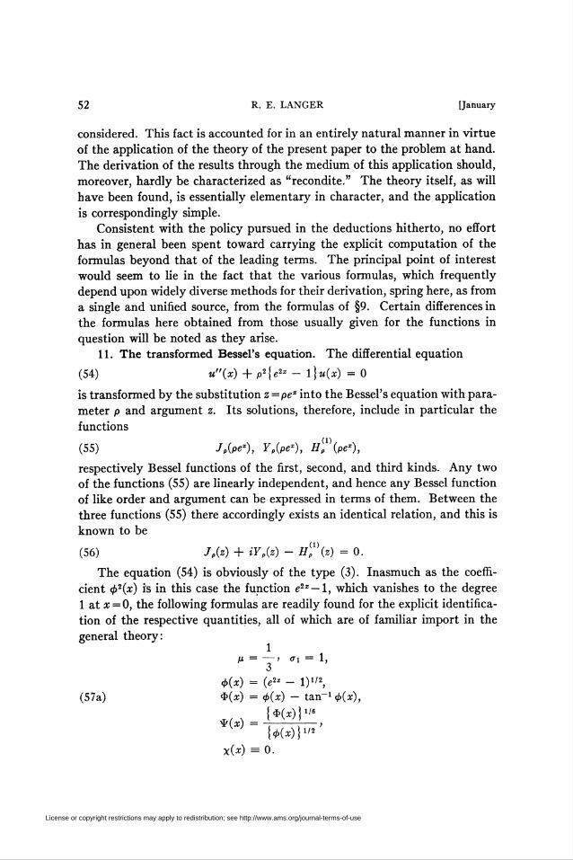
11. The transformed Bessel's equation. The differential equation
(54) u"(x) + p2{e2* - \)u(x) = 0
is transformed by the substitution z=pex into the Bessel's equation with para-
meter p and argument z. Its solutions, therefore, include in particular the
functions
(55) JP(pe*), Yp(Pe*), H?(pe*),
respectively Bessel functions of the first, second, and third kinds. Any two
of the functions (55) are linearly independent, and hence any Bessel function
of like order and argument can be expressed in terms of them. Between the
three functions (55) there accordingly exists an identical relation, and this is
known to be
(56) JP(z) + iYp(z) - H{p\z) = 0.
The equation (54) is obviously of the type (3). Inasmuch as the coeffi-
cient <p2(x) is in this case the function e2x— 1, which vanishes to the degree
1 at x = 0, the following formulas are readily found for the explicit identifica-
tion of the respective quantities, all of which are of familiar import in the
general theory:
P = —' <f\ — 1,
<p(x) = (e2* - l)1'2,
(57a) $(x) = <p(x) - ta,n-l<t>(x),
U(x)}1'6
{4>(x)V12
x(x) = 0.
License or copyright restrictions may apply to redistribution; see http://www.ams.org/journal-terms-of-use
1931] ASYMPTOTIC SOLUTIONS OF DIFFERENTIAL EQUATIONS 53
The hypotheses (i) to (iv) of §2 are found at a glance to be satisfied with
the interval / chosen as the entire axis of x, i.e., — °o <x<<*>. The admissi-
bility of this choice of an infinite interval and the corresponding availability
of the general results for all values of x depend further, therefore, only upon
the applicability of the hypothesis (v) of §7 to the case in hand. This applica-
bility may be investigated without difficulty by the procedure outlined as
follows. For values of x which are numerically large and respectively positive
or negative the function Q{x) defined in formula (5) may be expanded in
negative or positive powers of ex. It is found in this way that for x > 0,
tan 1 <b{x) vQ(x) = 1-— = 1-er* + e~2x + ■
*(*) 2
while for x<0,
«/ ■* < , * ~ loS U + i(t>(x)]n{x) = i -|-——-
t<p{x)
x< 1 + —e2x +•■>+ (1 - log 2) i 1 + — e2x +
By means of the formulas (12) and (23) it is now readily computed that for
positive values of x, 8{x)=0{l), and in consequence 9{x)/cp{x) =0{e~x),
whereas when x is negative 9{x) =0{x~2), and 9{x)/<p{x) =0{x~2). The hy-
pothesis (v) accordingly demands the convergence of a pair of integrals of
the type
Í 0{e~z)dx, \ oi—\dx, with c> 0,
and this requirement is clearly fulfilled.
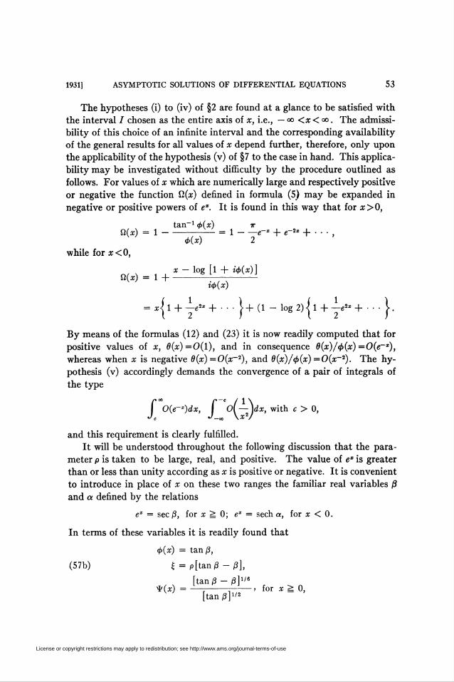
It will be understood throughout the following discussion that the para-
meter p is taken to be large, real, and positive. The value of ex is greater
than or less than unity according as x is positive or negative. It is convenient
to introduce in place of x on these two ranges the familiar real variables ß
and a defined by the relations
ex = sec ß, for x = 0; ex = sech a, for x < 0.
In terms of these variables it is readily found that
4>{x) = tan ß,
(57b) £ = P[tan/3-/3],
[tan ß - ß]116^{x) = —i--;-' f°r x = °»
[tan/3]1'2
License or copyright restrictions may apply to redistribution; see http://www.ams.org/journal-terms-of-use
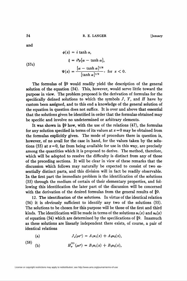
54 R. E. LANGER [January
and
<t>(x) = i tanh a,
£ = i3p[a — tanh a],
(57c)[a - tanh a]1'6
Sr'(x) = -:-:--i for X < 0.[tanh a]1'2
The formulas of §9 would readily yield the description of the general
solution of the equation (54). This, however, would serve little toward the
purpose in view. The problem proposed is the derivation of formulas for the
specifically defined solutions to Which the symbols /, F, and H have by
custom been assigned, and to this end a knowledge of the general solution of
the equation in question does not suffice. It is over and above that essential
that the solutions given be identified in order that the formulas obtained may
be specific and involve no undetermined or arbitrary elements.
It was shown in §9 how, with the use of the relations (47), the formulas
for any solution specified in terms of its values at x = 0 may be obtained from
the formulas explicitly given. The mode of procedure there in question is,
however, of no avail for the case in hand, for the values taken by the solu-
tions (55) at x = 0, far from being available for use in this way, are precisely
among the quantities which it is proposed to derive. The method, therefore,
which will be adopted to resolve the difficulty is distinct from any of those
of the preceding sections. It will be clear in view of these remarks that the
discussion which follows may naturally be expected to consist of two es-
sentially distinct parts, and this division will in fact be readily observable.
In the first part the immediate problem is the identification of the solutions
(55) through the medium of certain of their elementary properties, and fol-
lowing this identification the later part of the discussion will be concerned
with the derivation of the desired formulas from the general results of §9.
12. The identification of the solutions. In virtue of the identical relation
(56) it is obviously sufficient to identify any two of the solutions (55).
The solutions to be chosen for this purpose will be those of the first and third
kinds. The identification will be made in terms of the solutions Ui(x) and u2(x)
of equation (54) which are determined by the specifications of §9. Inasmuch
as these solutions are linearly independent there exists, of course, a pair of
identical relations
(a) J„(PeX) = AiUi(x) + A2Ui(x),
(58) (n(b) Hp (pe*) = Biui(x) + B2u2(x),
License or copyright restrictions may apply to redistribution; see http://www.ams.org/journal-terms-of-use
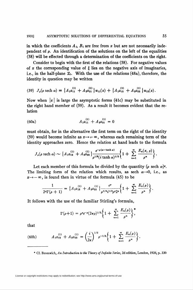
1931] ASYMPTOTIC SOLUTIONS OF DIFFERENTIAL EQUATIONS 55
in which the coefficients A,, B, are free from x but are not necessarily inde-
pendent of p. An identification of the solutions on the left of the equalities
(58) will be effected through a determination of the coefficients on the right.
Consider to begin with the first of the relations (58). For negative values
of x the corresponding value of £ lies on the negative axis of imaginaries,
i.e., in the half-plane Si. With the use of the relations (48a), therefore, the
identity in question may be written
(59) /p(psecha) m {Axaxl + A2a2X }ulx{x) + {AxaX2 + ^22 }uX2{x).
Now when \x | is large the asymptotic forms (41c) may be substituted in
the right hand member of (59). As a result it becomes evident that the re-
lation
(60a) Axaxx + A2a2X =0
must obtain, for in the alternative the first term on the right of the identity
(59) would become infinite as #—>• t- 00, whereas each remaining term of the
identity approaches zero. Hence the relation at hand leads to the formula
11 I. Ï ÍA (1)-l A (1)1 e^(<"taPhtt) L ^ En{x,p)\
Jl>{psecha)^{AxaX2 + A2a22\ A 1 + 2- -T~ \-p1/6(ttanha)1'2 v n=x P )
Let each member of this formula be divided by the quantity (p sech a)".
The limiting form of the relation which results, as sech a—>0, i.e., as
a;—> — 00, is found then in virtue of the formula (45) to be
1 ,, CD, . CD ) * Í, A £n(p)\-;- = {-4i<ii2 + A2a22 }——•-< 1 + ¿^ -> .2T(p + 1) pi/»iI'V2' l ÍÍ pn )
It follows with the use of the familiar Stirling's formula,
r(p+i) = p»e-'(2,rp)i/4l + ¿ ^1VK n=l Pn )
that
1/2 £n(p)'
(60b) A W A A (1) íl\ I/J1J V £"(P)l^4iai2 + A2a22 = ( — j p~ll3< 1 + 2-, ——?•
* Cf. Bromwich, An Introduction to the Theory of Infinite Series, 2d edition, London, 1926, p. 330
License or copyright restrictions may apply to redistribution; see http://www.ams.org/journal-terms-of-use
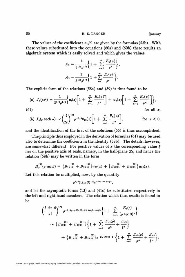
56 R. E. LANGER [January
The values of the coefficients o,i(1) are given by the formulas (53b). With
these values substituted into the equations (60a) and (60b) there results an
algebraic system which is easily solved and which gives the values
3"V'H „tí p» Í'
3'Vl ri P» J
The explicit form of the relations (58a) and (59) is thus found to be
« «* - ít^M1+s ~]+-4«+s ̂ ]}'(61) for all x,
■w r En(Py(b)
/ iv r °° -E (p)~\Jp(p sech a) ~ Í — j P-I'3ui2(x)\ 1 + £ —Ll I for x < 0,
and the identification of the first of the solutions (55) is thus accomplished.
The principle thus employed in the derivation of formulas (61) may be used
also to determine the coefficients in the identity (58b). The details, however,
are somewhat different. For positive values of x the corresponding value £
lies on the positive axis of reals, namely, in the half-plane So, and hence the
relation (58b) may be written in the form
Hp (psec/3) m {Biau + B2a2i }w0i(x) + {BiaX2 + B2a22 }w02(x).
Let this relation be multiplied, now, by the quantity
p1/6(tan ßyi2e-i,>{t™ß-ß)i
and let the asymptotic forms (13) and (41c) be substituted respectively in
the left and right hand members. The relation which thus results is found to
be
(2 sin ßyi2 ( » EJp) )I --\ p-l/3g-f>i(x/2-/3+tanß-Seoß) ) J _|_ \~\ _——_ >
\ ri I \ „_! (psecjS)"/
~\B^ + B¿£Úl+ t^^ + ̂ 1l „tí p» £" j
+ {Bia™ + B2a%}e-2^-4 1 + £ ^ + M.I „tí p" £» )
License or copyright restrictions may apply to redistribution; see http://www.ams.org/journal-terms-of-use
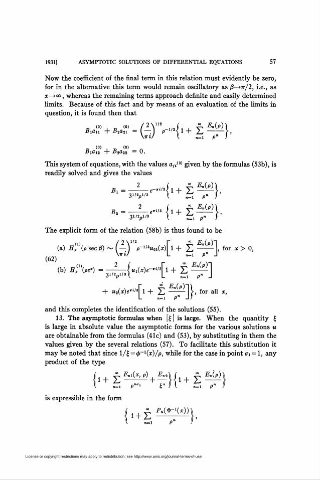
1931] ASYMPTOTIC SOLUTIONS OF DIFFERENTIAL EQUATIONS 57
Now the coefficient of the final term in this relation must evidently be zero,
for in the alternative this term would remain oscillatory as ß—>v/2, i.e., as
x—»oo, whereas the remaining terms approach definite and easily determined
limits. Because of this fact and by means of an evaluation of the limits in
question, it is found then that
Bxaxl + B2a2X = ( — 1 p 1/3< 1 + 2-» ——(>
(0) (0)BxaX2 + B2a22 = 0.
This system of equations, with the values a,¿(0) given by the formulas (53b), is
readily solved and gives the values
2 ( • En{p))
31V/S I tli p- J
The explicit form of the relation (58b) is thus found to be
(a) H™(p sec/3) ~ (AY V~lrtM*)[l + ¿ ~^\ for x > 0,
+ W2(x)e"/sri + ¿ ~rl}'for a11 *>
and this completes the identification of the solutions (55).
13. The asymptotic formulas when |£| is large. When the quantity £
is large in absolute value the asymptotic forms for the various solutions u
are obtainable from the formulas (41c) and (53), by substituting in them the
values given by the several relations (57). To facilitate this substitution it
may be noted that since l/£ = <p_1(a;)/p, while for the case in point ax = 1, any
product of the type
I n-l Pn'' £n ) l ZÍ p" )
is expressible in the form
( „_1 on I
(62)
License or copyright restrictions may apply to redistribution; see http://www.ams.org/journal-terms-of-use
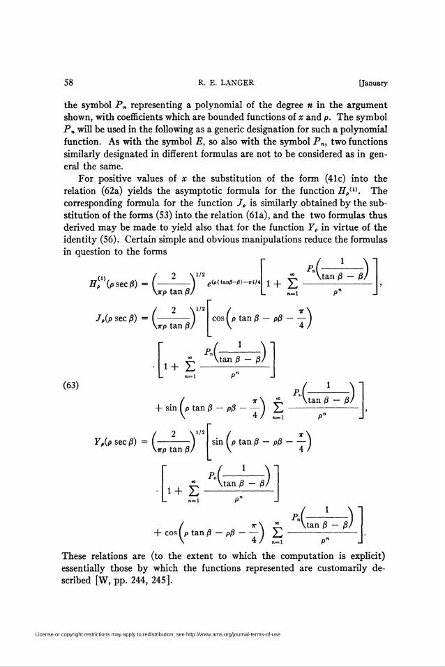
58 R. E. LANGER [January
the symbol P„ representing a polynomial of the degree n in the argument
shown, with coefficients which are bounded functions of x and p. The symbol
Pn will be used in the following as a generic designation for such a polynomial
function. As with the symbol E, so also with the symbol Pn, two functions
similarly designated in different formulas are not to be considered as in gen-
eral the same.
For positive values of x the substitution of the form (41c) into the
relation (62a) yields the asymptotic formula for the function Hpa). The
corresponding formula for the function /,, is similarly obtained by the sub-
stitution of the forms (53) into the relation (61a), and the two formulas thus
derived may be made to yield also that for the function Yp in virtue of the
identity (56). Certain simple and obvious manipulations reduce the formulas
in question to the forms
Vtan ß - ßlHp (p sec ß) -/_i-y,
\irp tan ß)
eip(tan/ä-i)-Tt/4l i+ £
/ 2 \1/2 / tt\J„(p sec ß) = I-1 cos I p tan ß — pß-)
\irp tan ßl V 4 /
i+ EVtan ß - ß)
(63)
+ sin í p tan ß — pß-j £
Y„(p sec ß) = (- ) sin ( p tan ß - pß - — )\tp tan ßl V 4 /
"Vtan ß - ßl
i-1—)Vtan ß - ßl
i+ £
<■4- cos I p tan ß — pß
4/ „_i
Vtan ß - ßl
These relations are (to the extent to which the computation is explicit)
essentially those by which the functions represented are customarily de-
scribed [W, pp. 244, 245].
License or copyright restrictions may apply to redistribution; see http://www.ams.org/journal-terms-of-use
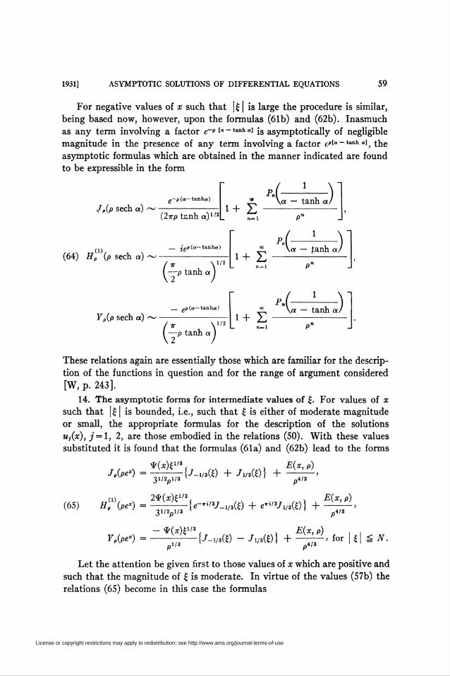
1931] ASYMPTOTIC SOLUTIONS OF DIFFERENTIAL EQUATIONS 59
For negative values of x such that | £ | is large the procedure is similar,
being based now, however, upon the formulas (61b) and (62b). Inasmuch
as any term involving a factor e~"la ~tanh al is asymptotically of negligible
magnitude in the presence of any term involving a factor e^a ~tanh al, the
asymptotic formulas which are obtained in the manner indicated are found
to be expressible in the form
J„{p sech a)
p—p(a— tanha)
,(1)(64) H„ (p sech a)
(2vp tanh a)1'2
_ Xop (a— tanha)
1+ £
p.(—*—)\a — tanh a/
Yp{p sech a)
(v y*I —p tanh a I
_ of> {a— tanha)
i+ z
Í —p tanh a 11/2
i+ T.
4 ' )\a — tanh a I
p-
>J ' )\a — tanh a)
These relations again are essentially those which are familiar for the descrip-
tion of the functions in question and for the range of argument considered
[W, p. 243].14. The asymptotic forms for intermediate values of £. For values of x
such that |£| is bounded, i.e., such that £ is either of moderate magnitude
or small, the appropriate formulas for the description of the solutions
ui{x), j = l, 2, are those embodied in the relations (50). With these values
substituted it is found that the formulas (61a) and (62b) lead to the forms
*(x)£1'3 . . E{x, p)
7>^ =1777^7 lJ-w® + Jl<3®} +
(65) H?\pe') =
YP{Pex) =
3i/y
2*(*)£1/3
„4/3
3l/2pl/3
- ^(*)£1'3
„1/3
{«-'</»/_!/,(£) +e'i/3Ji/3(£)} +E{x, p)
„4/3
. , E{x, p){/_!„(£) - /i/,«)} + ^y-, for | £| = N.
^4/3
Let the attention be given first to those values of x which are positive and
such that the magnitude of £ is moderate. In virtue of the values (57b) the
relations (65) become in this case the formulas
License or copyright restrictions may apply to redistribution; see http://www.ams.org/journal-terms-of-use
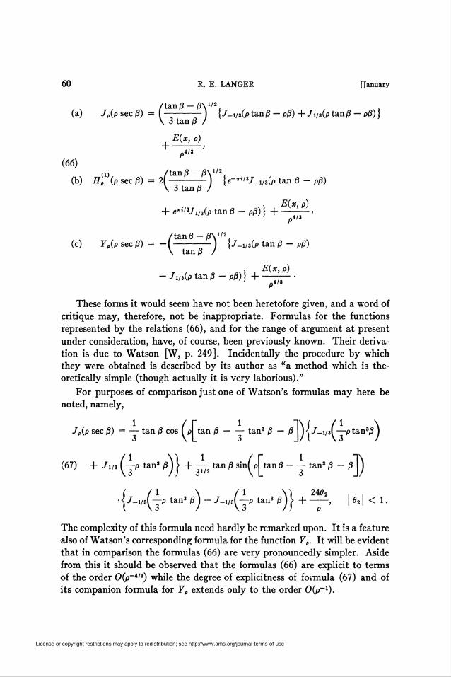
60 R. E. LANGER [January
/ta.nß-ß\ll2.(a) Jp(p sec ß) = I —-— \J-m(p tan/3 - pß) +Jm(P tan/? - pß)
\ 3 tan p /
, E(x,p)
p4l3
(66)(D /tan/3-jSX1'2
(b) Hp \p sec ß) = 2- {c-"/»/_v,(p tan ß - pß)V 3 tan /3 /3 tan/3
£(x, p)+ eTi/3/i/3(p tan /3 - p/3)} +
tan/3-/3\1/2
p4/3
/tan/3-/3y/2,(c) F,(p sec ß) = - ( —-— ) /-i/3(p tan ß
\ tan |3 /
- Jm(p tan /3 - pß) ) +
Pß)
E(x, p)
pU3
These forms it would seem have not been heretofore given, and a word of
critique may, therefore, not be inappropriate. Formulas for the functions
represented by the relations (66), and for the range of argument at present
under consideration, have, of course, been previously known. Their deriva-
tion is due to Watson [W, p. 249]. Incidentally the procedure by which
they were obtained is described by its author as "a method which is the-
oretically simple (though actually it is very laborious)."
For purposes of comparison just one of Watson's formulas may here be
noted, namely,
J„(p sec ß) = — tan ß cos ( p tan ß-tan3 ß - ß K7_i/3Í— ptan3/? J
(67) + Ji/3 (~p tan3 ß H + — tan ß sinf p tan/3-tan3 ß - ß j
•i/_1/3f—p tan3 ß\ - J-iJ—p tan3 ßj\2402 . ,
+-, le, < i.
The complexity of this formula need hardly be remarked upon. It is a feature
also of Watson's corresponding formula for the function Y„. It will be evident
that in comparison the formulas (66) are very pronouncedly simpler. Aside
from this it should be observed that the formulas (66) are explicit to terms
of the order 0(p~413) while the degree of explicitness of formula (67) and of
its companion formula for Yp extends only to the order 0(p~x).
License or copyright restrictions may apply to redistribution; see http://www.ams.org/journal-terms-of-use
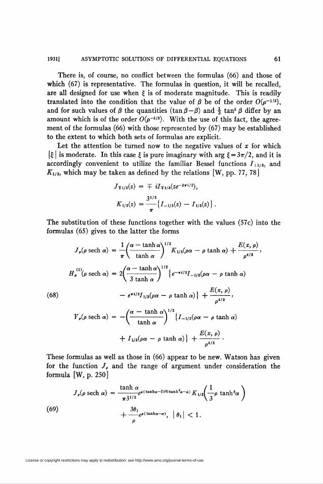
1931] ASYMPTOTIC SOLUTIONS OF DIFFERENTIAL EQUATIONS 61
There is, of course, no conflict between the formulas (66) and those of
which (67) is representative. The formulas in question, it will be recalled,
are all designed for use when £ is of moderate magnitude. This is readily
translated into the condition that the value of ß be of the order 0{p~113),
and for such values of ß the quantities (tan/3—ß) and f tan3 ß differ by an
amount which is of the order 0{p~613). With the use of this fact, the agree-
ment of the formulas (66) with those represented by (67) may be established
to the extent to which both sets of formulas are explicit.
Let the attention be turned now to the negative values of x for which
|£ | is moderate. In this case £ is pure imaginary with arg £ = 3ît/2, and it is
accordingly convenient to utilize the familiar Bessel functions I±i/t, and
Kx/i, which may be taken as defined by the relations [W, pp. 77, 78]
7¥V8(z) = + îTTi/3(ze-3'i'2),
Kx/3{z) =-{J_i/,(s) -JV««}.V
The substitution of these functions together with the values (57c) into the
formulas (65) gives to the latter the forms
E{x, p)1/a-tanha\1/2 E{x,Jf,{p sech a) = —I-) KX/3{pa — p tanh a) -\-
v \ tanh a / p4/
1/2
;3
(i) ¡a — tanhaX1'2,H„ (p sech a) = 21-) {e-Ti/3/_i/3(pa - p tanh a)
\ 3 tanh a /
E{x, p)(68) - eri'3Ix/3{pa - p tanh a)} +
p4/3
(a — tanh a\1/2(Y„{p sech a) = —I-1 {7_i/3(pa — p tanh a)
\ tanh a /
E{x, p)+ Ix/3{pa — p tanh a) \ +
pin
These formulas as well as those in (66) appear to be new. Watson has given
for the function Jp and the range of argument under consideration the
formula [W, p. 250]
tanh a , / 1 \/„(pSecha) = -^(tanha-OWtanhV-a)^ (_ tanh3a )
T31'2 \ 3 /
(69) 301_|-ep(tanha-af); | 0j | < 1 .
P
License or copyright restrictions may apply to redistribution; see http://www.ams.org/journal-terms-of-use
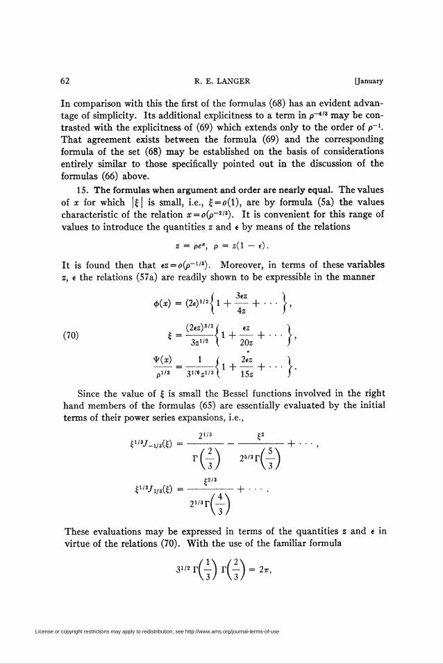
62 R. E. LANGER [January
In comparison with this the first of the formulas (68) has an evident advan-
tage of simplicity. Its additional explicitness to a term in p~*13 may be con-
trasted with the explicitness of (69) which extends only to the order of p-1.
That agreement exists between the formula (69) and the corresponding
formula of the set (68) may be established on the basis of considerations
entirely similar to those specifically pointed out in the discussion of the
formulas (66) above.
15. The formulas when argument and order are nearly equal. The values
of x for which |£| is small, i.e., £ = o(l), are by formula (5a) the values
characteristic of the relation x = o(p~213). It is convenient for this range of
values to introduce the quantities z and e by means of the relations
z = pex, p = z(l — e).
It is found then that ez = o(p~113). Moreover, in terms of these variables
z, e the relations (57a) are readily shown to be expressible in the manner
( 3ez4>(x) = (2e)1'*« 1 +-+ • ■
{ 4z
(2íz)3'2 ( ez )
(70) {~5=r{1+5.+ -}'
(x) 1 t 2tz \— =-< i +— + ••• \1/3 31/6z1/3l 15z j
^(x)
p
Since the value of £ is small the Bessel functions involved in the right
hand members of the formulas (65) are essentially evaluated by the initial
terms of their power series expansions, i.e.,
2l/3 £2
el3J-xn(& =-—-—— + • • • ,
(!) 2"*r(7)
£2/3
i"'/i/i(f)-— + • • ■ .
These evaluations may be expressed in terms of the quantities z and « in
virtue of the relations (70). With the use of the familiar formula
"KiMi)¿T,
License or copyright restrictions may apply to redistribution; see http://www.ams.org/journal-terms-of-use
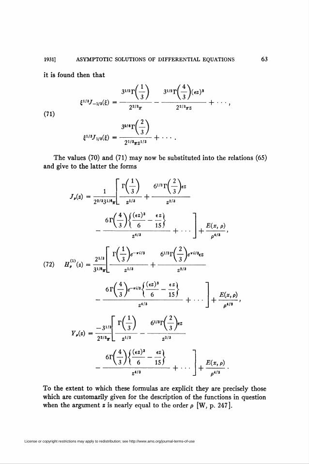
1931] ASYMPTOTIC SOLUTIONS OF DIFFERENTIAL EQUATIONS
it is found then that
63
31/2r
£"3/-i/3(£) =
(I) 3miiYzy
(71)22'3x
36/6r
22/Vz+
£1/3/i/3(£) -(I)
21/3xZl/3+
The values (70) and (71) may now be substituted into the relations (65)
and give to the latter the forms
J„{z) =1
22'331'i7r *l/3 „2/3
«G){4\f(«)» tz\
+ +E{x, p)
,4/S
(i) 21'3
\~ie~ri" 6li*r(—\
7i/3 „2/3
/4\ ({ez)3 tz)
»4/3+ +
E{x,p)
„4/3
y m =_3!/3
22/37T
'(I) 6"'r(j>
,1/3Z1" 22/3
,4/3+ +
£(*, P)
r>4/3
To the extent to which these formulas are explicit they are precisely those
which are customarily given for the description of the functions in question
when the argument z is nearly equal to the order p [W, p. 247].
License or copyright restrictions may apply to redistribution; see http://www.ams.org/journal-terms-of-use
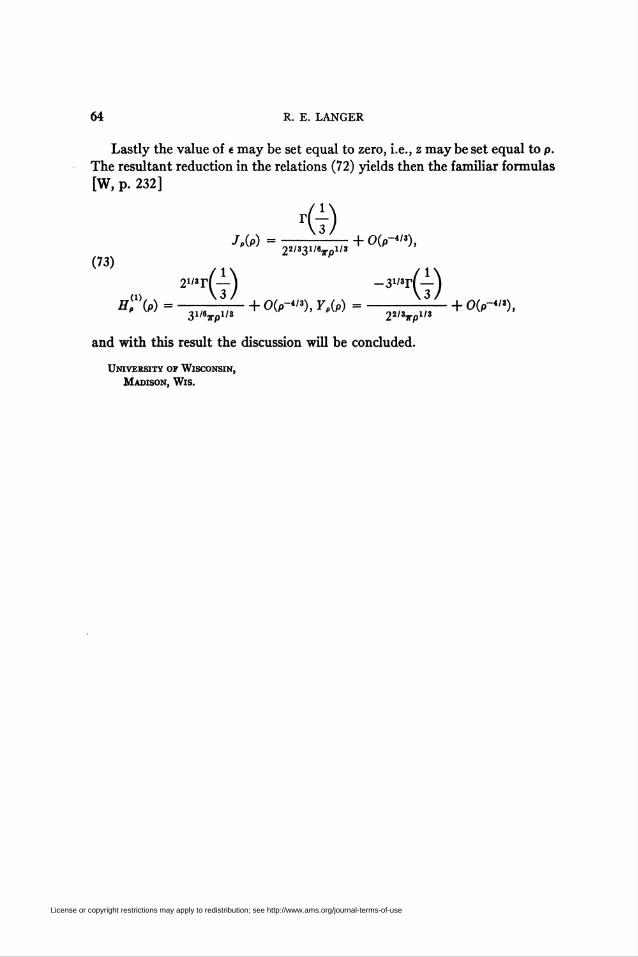
64 R. E. LANGER
Lastly the value of e may be set equal to zero, i.e., z may be set equal to p.
The resultant reduction in the relations (72) yields then the familiar formulas
[W, p. 232]
<7)Jp(p) =-r- 0(p-4/3),
p 22/331/fW3
(73)2i/sr
(t) , -3"'<t)fl"'w - -¡553- + °™ *M —^r- + 0('-,">.
and with this result the discussion will be concluded.
University of Wisconsin,
Madison, Wis.
License or copyright restrictions may apply to redistribution; see http://www.ams.org/journal-terms-of-use


![Fourier-Bessel Analysis of Cyllindrically Symmetric ... · other members of professor Gauthier’s group using Bessel-Legendre-Fourier technique [8]. By using a Fourier-Bessel set](https://img.pdfslide.us/doc/110x75/5f5e2e5a108c766ffb3ab4fc/fourier-bessel-analysis-of-cyllindrically-symmetric-other-members-of-professor.jpg)


![Coulomb and Bessel Functions of Complex Arguments and … · COMPLEX COULOMB AND BESSEL FUNCTIONS ... and the Fourier-Bessel equation [13] and many others, e.g., ... and gave tables](https://img.pdfslide.us/doc/110x75/5af3f2587f8b9a92718cd9fc/coulomb-and-bessel-functions-of-complex-arguments-and-coulomb-and-bessel-functions.jpg)